gene expression data analysis guidelines - … · man-c0011-04 gene expression data analysis...

MAN-C0011-04 Gene Expression Data Analysis Guidelines

FOR RESEARCH USE ONLY. Not for use in diagnostic procedures

© 2017 NanoString Technologies, Inc. All rights reserved. NanoString, NanoString Technologies, the NanoString logo, nCounter, and nSolver are trademarks or registered trademarks of NanoString Technologies, Inc., in the United States and/or other countries

Gene Expression Data Analysis Guidelines

Purpose

This document describes recommended procedures for the analysis of nCounter® gene expression assays. It can serve either as a stand-alone guide for analyzing nCounter datasets using a third-party software package, or it may be utilized as a companion guide to our own nSolver™ Analysis Software (https://www.nanostring.com/products/analysis-software/nsolver, Getting Started tab). The following content mirrors the available tools and options within nSolver, and contains brief “break-out boxes” illustrating how to implement a subset of these options in this Analysis Software. For a shorter overview of workflow without any accompanying recommendations, refer to the Quick Start Guide to nSolver, or, for a more comprehensive guide on the execution of all nSolver features, see the full nSolver Analysis Software User Manual (https://www.nanostring.com/products/analysis-software/nsolver, Support Documents tab).

Introduction

Gene expression assays on the nCounter system provide reliable, sensitive, and highly-multiplexed detection of mRNA targets. These assays are usually performed without the use of enzymes or amplification protocols, and do not rely on degree of fluorescence intensity to determine target abundance. These characteristics, combined with the highly-automated nature of barcoded sample processing, result in a platform that yields data which is both precise and reproducible. Nevertheless, it is prudent to follow procedures outlined herein to ensure that you are generating the highest data quality possible.

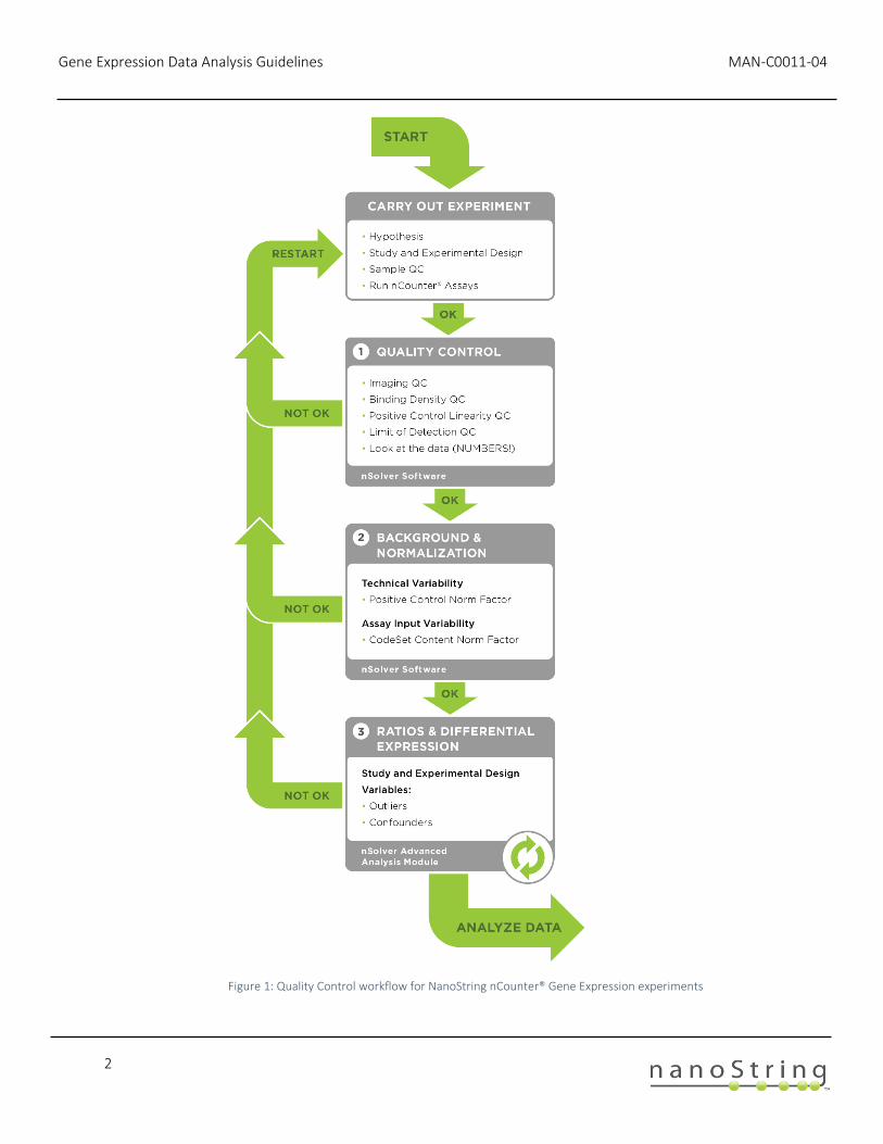
Figure 1 shows a general workflow for analyzing an nCounter gene expression experiment. In an iterative process, data quality is assessed after every stage of analysis. We start by evaluating the general assay performance using Quality Control (QC) metrics recorded in the nCounter data files (RCC files). Afterwards, we perform Background correction and data Normalization followed by another round of data QC. Finally, we assess the resulting Ratios, Fold-Changes and Differential Expression, and these results, too, should be carefully checked for quality control characteristics.

https://www.nanostring.com/products/analysis-software/nsolver

https://www.nanostring.com/products/analysis-software/nsolver

Gene Expression Data Analysis Guidelines MAN-C0011-04

2

Figure 1: Quality Control workflow for NanoString nCounter® Gene Expression experiments


3

Quality Control To ensure that data resulting from an nCounter Gene Expression experiment on the nCounter analysis

system is of substantial quality to be used in a subsequent in-depth statistical analysis, it is necessary to

perform a thorough quality control check on that data. In this section, we address Quality Control (QC) for

General Assay Performance.

We start checking the overall performance of the nCounter assay by evaluating the Imaging and Binding Density QC metrics. Next, we assess the performance of the positive controls using the Positive Control Linearity and Limit of Detection parameters. Finally, we do an overall visual inspection of the data and assess the severity of any QC flags.

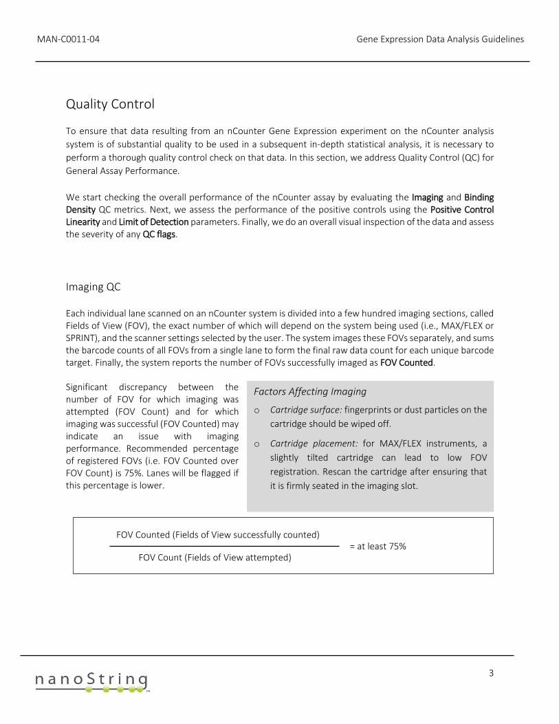
Imaging QC Each individual lane scanned on an nCounter system is divided into a few hundred imaging sections, called Fields of View (FOV), the exact number of which will depend on the system being used (i.e., MAX/FLEX or SPRINT), and the scanner settings selected by the user. The system images these FOVs separately, and sums the barcode counts of all FOVs from a single lane to form the final raw data count for each unique barcode target. Finally, the system reports the number of FOVs successfully imaged as FOV Counted. Significant discrepancy between the number of FOV for which imaging was attempted (FOV Count) and for which imaging was successful (FOV Counted) may indicate an issue with imaging performance. Recommended percentage of registered FOVs (i.e. FOV Counted over FOV Count) is 75%. Lanes will be flagged if this percentage is lower.

FOV Count (Fields of View attempted)

FOV Counted (Fields of View successfully counted) = at least 75%

Factors Affecting Imaging

o Cartridge surface: fingerprints or dust particles on the

cartridge should be wiped off.

o Cartridge placement: for MAX/FLEX instruments, a

slightly tilted cartridge can lead to low FOV

registration. Rescan the cartridge after ensuring that

it is firmly seated in the imaging slot.


4

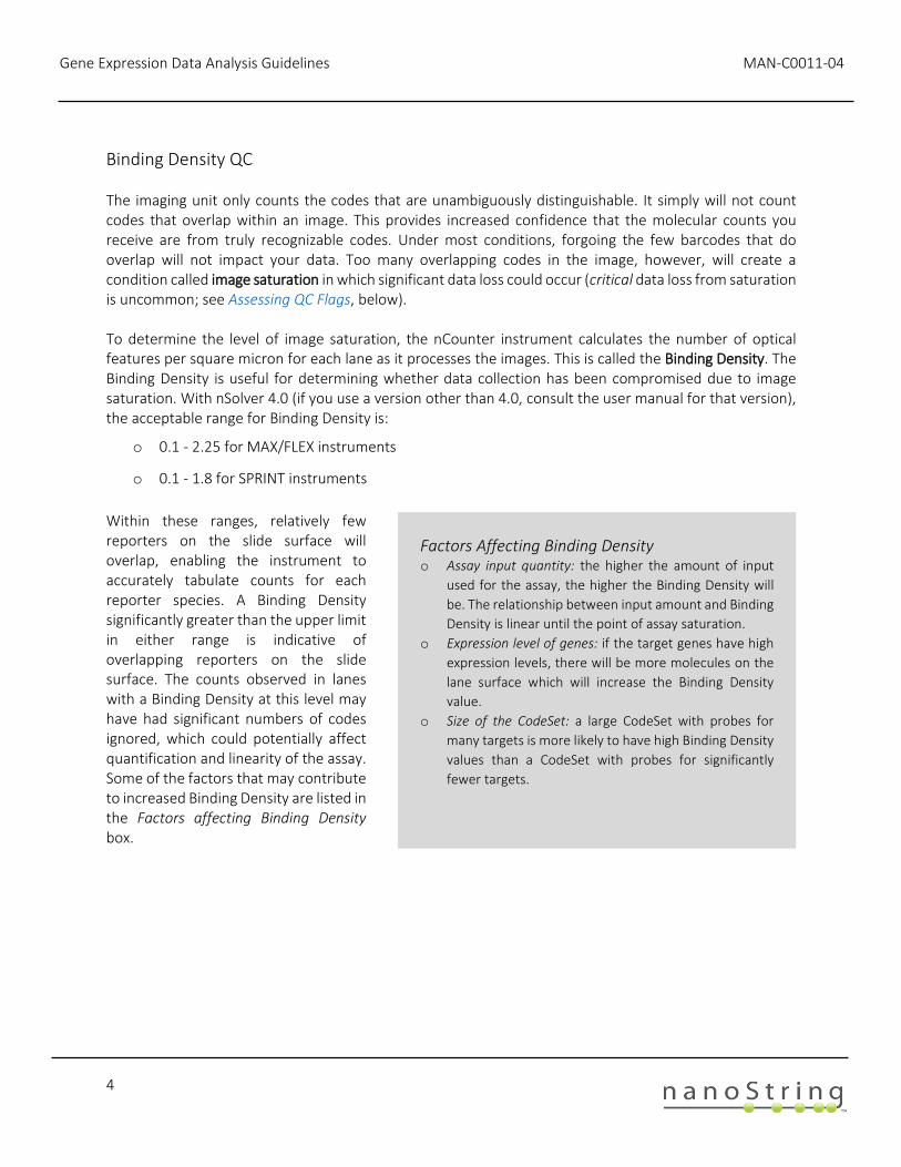
Binding Density QC The imaging unit only counts the codes that are unambiguously distinguishable. It simply will not count codes that overlap within an image. This provides increased confidence that the molecular counts you receive are from truly recognizable codes. Under most conditions, forgoing the few barcodes that do overlap will not impact your data. Too many overlapping codes in the image, however, will create a condition called image saturation in which significant data loss could occur (critical data loss from saturation is uncommon; see Assessing QC Flags, below). To determine the level of image saturation, the nCounter instrument calculates the number of optical features per square micron for each lane as it processes the images. This is called the Binding Density. The Binding Density is useful for determining whether data collection has been compromised due to image saturation. With nSolver 4.0 (if you use a version other than 4.0, consult the user manual for that version), the acceptable range for Binding Density is:

o 0.1 - 2.25 for MAX/FLEX instruments

o 0.1 - 1.8 for SPRINT instruments

Within these ranges, relatively few reporters on the slide surface will overlap, enabling the instrument to accurately tabulate counts for each reporter species. A Binding Density significantly greater than the upper limit in either range is indicative of overlapping reporters on the slide surface. The counts observed in lanes with a Binding Density at this level may have had significant numbers of codes ignored, which could potentially affect quantification and linearity of the assay. Some of the factors that may contribute to increased Binding Density are listed in the Factors affecting Binding Density box.

Factors Affecting Binding Density o Assay input quantity: the higher the amount of input

used for the assay, the higher the Binding Density will

be. The relationship between input amount and Binding

Density is linear until the point of assay saturation.

o Expression level of genes: if the target genes have high

expression levels, there will be more molecules on the

lane surface which will increase the Binding Density

value.

o Size of the CodeSet: a large CodeSet with probes for

many targets is more likely to have high Binding Density

values than a CodeSet with probes for significantly

fewer targets.


5

Positive Control Linearity QC Six synthetic DNA control targets are included with every nCounter Gene Expression assay. Their concentrations range linearly from 128 fM to 0.125 fM, and they are referred to as POS_A to POS_F, respectively. These positive controls are typically used to measure the efficiency of the hybridization reaction, and their step-wise concentrations also make them useful in checking the linearity performance of the assay. An R2 value is calculated from the regression between the known concentration of each of the positive controls and the resulting counts from them (this calculation is performed using log2-transformed values).

Since the known concentrations of the positive controls increase in a linear fashion, the resulting counts should, as well. Therefore, R2 values should be higher than 0.95. Note that because POS_F has a known concentration of 0.125 fM, which is considered below the limit of detection of the system, it should be excluded from this calculation (although you will see that POS_F counts are significantly higher than the negative control counts in most cases).

Log2 Known [positive controls]

Log2 Measured [positive controls] > 0.95 R2 = linear regression of

Factors Affecting POS Control Linearity

o Probe vs sample interactions: Uncommonly, a single

positive control probe will show unusually high or low

counts, usually because of an interaction between this

probe and a sample, which will not manifest during

NanoString manufacturing QC. This will usually have

little to no effect on data quality.

o Very low assay efficiency: If the counts of all the positive

controls are very low (less than ~500 even for POS_A),

linearity will be compromised. This is usually the result

of a critical assay failure and data will likely be

compromised.


6

Limit of Detection QC The limit of detection is determined by measuring the ability to detect POS_E, the 0.5 fM positive control probe, which corresponds to about 10,000 copies of this target within each sample tube. On a FLEX/MAX system, the standard input of 100 ng of total RNA will roughly correspond to about 10,000 cell equivalents (assuming one cell contains 10 pg total RNA on average). An nCounter assay run on the FLEX/MAX system should thus conservatively be able to detect roughly 1 transcript copy per cell for each target (or 10,000 total transcript copies). In most assays, you will observe that even the POS_F probe (equivalent to 0.25 copies per cell) is detectable above background. To determine whether POS_E is detectable, it can be compared to the counts for the negative control probes. Every nCounter Gene Expression assay is manufactured with eight negative control probes that should not hybridize to any targets within the sample. Counts from these will approximate general non-specific binding of probes within the samples being run. The counts of POS_E should be higher than two times the standard deviation above the mean of the negative control.

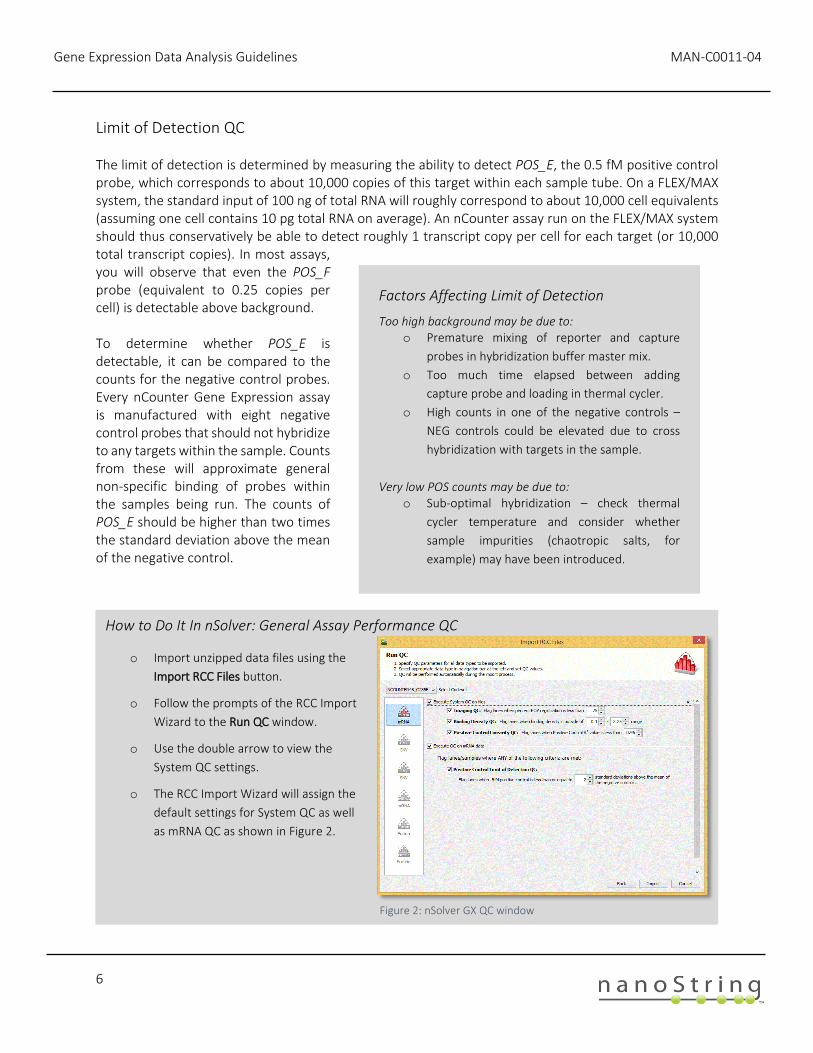
How to Do It In nSolver: General Assay Performance QC

Factors Affecting Limit of Detection

Too high background may be due to: o Premature mixing of reporter and capture

probes in hybridization buffer master mix.

o Too much time elapsed between adding

capture probe and loading in thermal cycler.

o High counts in one of the negative controls –

NEG controls could be elevated due to cross

hybridization with targets in the sample.

Very low POS counts may be due to: o Sub-optimal hybridization – check thermal

cycler temperature and consider whether

sample impurities (chaotropic salts, for

example) may have been introduced.

o Import unzipped data files using the

Import RCC Files button.

o Follow the prompts of the RCC Import

Wizard to the Run QC window.

o Use the double arrow to view the

System QC settings.

o The RCC Import Wizard will assign the

default settings for System QC as well

as mRNA QC as shown in Figure 2.

Figure 2: nSolver GX QC window


7

Assessing QC Flags The recommended quality control specifications for NanoString data are designed to highlight samples that have moderate-to-severe reductions in assay efficiency or data quality. Some samples that do not pass quality control may still provide robust count data, but they are singled out to highlight a potential cause of poor assay efficiency that could result in data loss in future assays. Even if the data from these samples is usable, it is a good practice to determine the root cause of all such detectable changes in assay efficiency. For tips on how to assess these root causes, see the Factors Affecting … boxes for each QC parameter section, above. NanoString Technical Services ([email protected]) and/or your Field Application Scientist can also assist you with troubleshooting, if necessary.

Samples with lowered assay efficiency (or with reduced quality or quantity of RNA) will also exhibit lowered raw counts for probes in the NanoString CodeSet. Depending on how background correction and normalization is performed, low expressing targets in these samples will either fail to be detected (false negatives) or will have higher-than-expected counts (false positives). To determine whether it would be necessary to discard the data from flagged samples, see the sections below for some rough guidelines to use.

Examine the Positive and Negative Controls

o If samples were flagged because a single positive or negative control probe was much different

than expected (leading to positive control linearity flag or Limit of Detection flag), it is very likely

the data from that sample is still usable.

o If all the positive controls are extremely low, such that most (if not all) are close to the background

(negative control probe counts), assay linearity and/or sensitivity are likely compromised and such

samples may not provide robust data.

Examine the Calculated QC Metrics

o If the QC metrics fail the flag threshold by a very small margin (i.e., FOV registration was 72%, just

below the 75% recommended cut off), the data is likely robust and usable.

o Conversely, samples with QC metrics which miss the cutoff by a wide margin (i.e., FOV registration

was 11% instead of >75%), will usually not provide robust data. NOTE: Binding density flags seldom

result in critical data loss; use the Visually Inspect the Data and the Identify Outlier Samples sections

below, especially when the Binding Density threshold has been exceeded by a considerable margin.

mailto:[email protected]


8

Visually Inspect the Data

o A simple inspection of the data may either identify problematic samples or give greater confidence

that data for the sample in question is sufficiently robust for downstream inclusion.

o Samples may need to be excluded if an inspection of raw counts indicates that substantially fewer

genes are being detected above the background (negative control) probes compared to other

samples from a similar treatment group.

o Samples may need to be excluded if an inspection of normalized counts indicates that substantially

more genes are being detected above the background probes compared to other samples from

the same treatment group. NOTE: The Background Thresholding option in nSolver will prevent

these false positives from showing up; this approach is not recommended if Background

Thresholding has been performed on the data.

Identify Outlier Samples

o Instead of a visual inspection, various methods may be used to identify outlier samples, which may

be indicative of assay- or sample-level problems which necessitate removal of such data from

downstream analyses.

o One way to identify outlier samples is to generate a heat map of normalized data from all samples.

If the flagged samples in question are strongly divergent from other samples with similar pathology,

they may need to be removed from further analyses. In nSolver, you will need to proceed through

the steps to create an experiment before doing a heat map Analysis, at which point you can refer

to the Agglomerative Cluster (Heat Map) section in the nSolver User Manual.

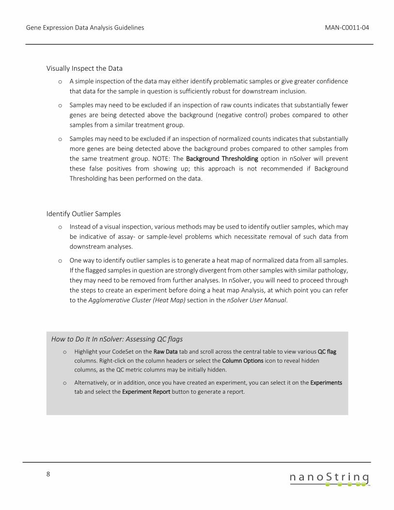
How to Do It In nSolver: Assessing QC flags

o Highlight your CodeSet on the Raw Data tab and scroll across the central table to view various QC flag

columns. Right-click on the column headers or select the Column Options icon to reveal hidden

columns, as the QC metric columns may be initially hidden.

o Alternatively, or in addition, once you have created an experiment, you can select it on the Experiments

tab and select the Experiment Report button to generate a report.


9

Background Correction

Despite the high specificity of nCounter probes, very low levels of non-specific counting are still inherent

to any NanoString assay. Thus, a small number of counts for each of the targets in a CodeSet will represent

false positives. Typically, we do not recommend correcting for non-specific counting since true counts for

most mRNA targets will far outnumber false positives, and thus the effects of the latter on fold-change

estimates will be negligible. However, for those projects where low expressing targets are common, or

when the presence or absence of a transcript has an important research implication, it may be useful to

more precisely delineate which counts are false positives. For these reasons, we introduce two methods

of background correction: Background Thresholding and Background Subtraction. We also describe three

different approaches in establishing a value to use in conjunction with thresholding or subtraction: using

the Negative Control Probes, a Fixed Background, or a Negative Control Sample.

Background Threshold

Background thresholding is a process whereby a threshold value is set and all counts which fall below that

value are adjusted to match it. When data is background subtracted (see next section), in contrast, non-

specific counts are subtracted from the raw counts to obtain a new estimate of counts above background.

For most studies of gene expression where fold-change estimations are an important result, background

thresholding is preferred over background subtraction. This is because the latter tends to substantially

overestimate fold-changes in low-expressing targets; background subtracted counts for low-expressing

targets can be close to zero, potentially setting either the numerator or denominator of the fold-change

calculation to a very small number. The biological importance of large absolute fold-changes in background

subtracted data may be overestimated when the expression level of the gene is close to the background.

Background Subtraction

If, instead of fold-changes, estimates of counted transcripts above background noise are an important

result, then you may consider using background subtraction. Consider, however, the following cautionary

notes about background subtraction values in nSolver:

o Because the nSolver math engine operates in log2 space, any counts below 1 (including negative

counts) will be reset to 1.0. Thus, counts which appear as 1.0 in nSolver output will frequently

represent counts less than 1.

o Background subtracted values may subsequently be multiplied by normalization scaling factors.

Particularly for samples with normalization flags, some targets below background will be

normalized to potentially large values depending on the size of the scaling factors, and thus may

appear to be much higher than background. Counts in nSolver which have been set to the

background threshold will not be altered further during normalization.


10

Negative Control Probes

Every nCounter CodeSet or TagSet is manufactured to contain 6 or 8 negative control probes, designated

by the probe name, Negative A (NEG_A), Negative B (NEG_B), etc. These control probes are designed

against engineered RNA sequences (ERCC RNA controls) which are not present in biological samples.

Negative control probes are commonly used to set background thresholds.

Every probe in an nCounter assay will exhibit some variability in non-specific counting. By observing this

variability among the negative control probe targets, we can predict the level of variability in baseline non-

specific counts that we expect to see for the endogenous and housekeeping targets.

We can use the mean, mean plus standard deviation, median, geometric mean, or maximum of the

negative control counts. The level of stringency used in setting this threshold will affect the balance

between false positive and false negative target occurrences. Examples of metrics you can use and their

potential implications include:

o You can minimize the number of false positives by setting the threshold to the mean plus two

standard deviations or to the maximum of the negative control counts; note, however, that

although false positives will be rare, false negatives may be relatively abundant.

o Conversely, you can set a more liberal threshold, such as the geometric mean of the negative

controls. This will increase the number of false positives, but simultaneously decrease the number

of false negatives.

Fixed Value Background

Another approach to setting the background is to simply define a fixed value. This would only be

appropriate if previous experiments had identified a robust measure of probe non-specific binding that met

the project qualifications for target exclusion. Used in conjunction with background thresholding, all

targets with raw counts equal to or less than this defined value would be set to this value. Used with

background subtraction, this defined value would be subtracted from the raw counts of all targets.

Rare Negative Control Deviations

Rarely, unique and difficult-to-predict probe-to-probe interactions may occur, resulting in one or

two negative control probes being more than 3-fold higher than all the other negative control

probes. It is acceptable to remove these outliers for purposes of background threshold or

background subtraction.


11

Negative Control Sample

One limitation of the previously-described approaches (negative controls or a fixed value) is that some

proportion of false positives or false negatives are expected, given the variance in non-specific counting

across probes. One approach to defining background more precisely would be to run samples which

contain no target transcripts, such as an RNA-free water sample. This would require using one or more

sample lanes per project (not per cartridge) for these negative control samples in lieu of experimental

samples. Ideally, three negative control samples would be run for each build of a CodeSet, and a t-test

performed for each target transcript. These three negative control replicates would then be compared to

the biological replicates run within each of the other treatment groups.

How to Do It In nSolver: Background Thresholding

o Create an experiment and follow

the Experiment Wizard prompts

to the Background

Subtraction/Thresholding screen.

o Check the box for Background

Subtraction/Thresholding.

o Check the box for Negative

control count.

o Set the Threshold to mean +2

standard deviations above the

mean.

Figure 3: nSolver background settings window


12

Normalization

Data normalization is designed to remove sources of technical variability from an experiment, so that the

remaining variance can be attributed to the underlying biology of the system under study. The precision

and accuracy of nCounter Gene Expression assays are dependent upon robust methods of normalization

to allow direct comparison between samples. There are many sources of technical variability that can

potentially be introduced into nCounter assays. The largest and most common categories of variability

originate from either the platform or the sample. We describe how both types of variability can be

normalized using standard normalization procedures for Gene Expression assays.

Standard normalization uses a combination of Positive

Control Normalization, which uses synthetic positive control

targets, and CodeSet Content Normalization, which uses

housekeeping genes, to apply a sample-specific correction

factor to all the target probes within that sample lane. These

correction factors will control for all those technical sources

of variability which should affect all the probes equally,

compensating for sources of error including pipetting errors,

instrument scan resolution, lot-to-lot variation in Prep Plates

and Cartridges, and sample input variability. These

procedures are effective as long as the CodeSets or probes

themselves are derived from the same manufacturing lot (if

not, see the Lot to Lot Variation in Probes box).

Note that positive control normalization will not correct for

sample input variability, and thus should usually be used in

combination with CodeSet Content (housekeeping gene)

Normalization. Performing such a two-step normalization

will usually not differ mathematically from Content

Normalization alone, and thus is mathematically somewhat

redundant. Nevertheless, normalizing to both target classes

will provide a good indicator of how technical variability is

partitioned between the two major sources of assay noise

(platform and sample), and thus may provide a good tool for

troubleshooting low assay performance. Below, we describe

both types of normalization, as well as Normalization QC.

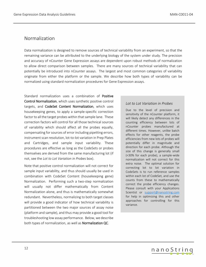
Lot to Lot Variation in Probes

Due to the level of precision and sensitivity of the nCounter platform, it will likely detect any differences in the counting efficiency between lots of nCounter probes manufactured at different times. However, unlike batch effects for other reagents, the probe efficiencies from new lots of probes will potentially differ in magnitude and direction for each probe. Although the size of this change is generally small (<30% for each probe), a sample-wide normalization will not correct for this extra noise. The optimal solution for correcting lot to lot variation in CodeSets is to run reference samples within each lot of CodeSet, and use the counts from these to mathematically correct the probe efficiency changes. Please consult with your Applications Scientist or [email protected] for help in optimizing this and other approaches for controlling for this variance.



13

Positive Control Normalization

nCounter Reporter probe (or TagSet) tubes are manufactured to contain six synthetic ssDNA control targets.

The counts from these targets may be used to normalize all platform-associated sources of variation (e.g.,

automated purification, hybridization conditions, etc.).

Although the calculations are performed automatically in nSolver, the procedure is as follows (see Figure

5):

1. Calculate the geometric mean (Geomean) of the positive controls for each lane.

2. Calculate the arithmetic

mean of these geometric

means for all sample lanes.

3. Divide this arithmetic

mean by the geometric

mean of each lane to

generate a lane-specific

normalization factor.

4. Multiply the counts for

every gene by its lane-

specific normalization

factor.

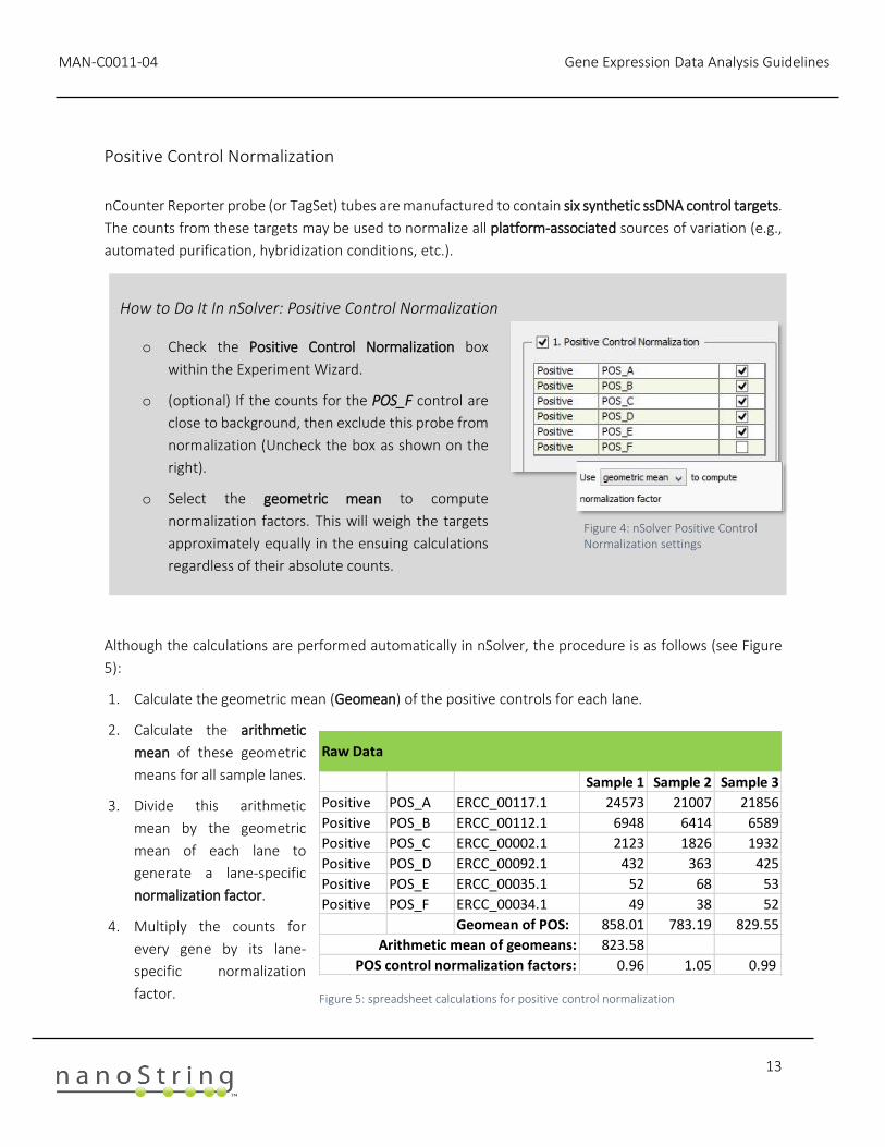
How to Do It In nSolver: Positive Control Normalization

o Check the Positive Control Normalization box

within the Experiment Wizard.

o (optional) If the counts for the POS_F control are

close to background, then exclude this probe from

normalization (Uncheck the box as shown on the

right).

o Select the geometric mean to compute

normalization factors. This will weigh the targets

approximately equally in the ensuing calculations

regardless of their absolute counts.

Figure 1 Default recommendations for positive

control normalization

Figure 1 Default recommendations for positive

control normalization

Figure 4: nSolver Positive Control Normalization settings

Raw Data

Sample 1 Sample 2 Sample 3

Positive POS_A ERCC_00117.1 24573 21007 21856

Positive POS_B ERCC_00112.1 6948 6414 6589

Positive POS_C ERCC_00002.1 2123 1826 1932

Positive POS_D ERCC_00092.1 432 363 425

Positive POS_E ERCC_00035.1 52 68 53

Positive POS_F ERCC_00034.1 49 38 52

Geomean of POS: 858.01 783.19 829.55

Arithmetic mean of geomeans: 823.58

POS control normalization factors: 0.96 1.05 0.99

Figure 5: spreadsheet calculations for positive control normalization


14

CodeSet Content or Housekeeping Gene Normalization

It is expected that some noise will invariably be introduced into the nCounter assay due to variability in

sample input. Since it is not always practical to measure real world samples with the precision and accuracy

necessary to ensure that each lane contains the same amount and quality of RNA, it is desirable to correct

for this variability. We can do this by normalizing to a surrogate measure of total RNA input into the assay.

For most experiments run on the nCounter platform, this is most effectively done using so-called

housekeeping genes; these are mRNA targets included in a CodeSet which are known to or suspected to

show little-to-no variability in expression across all treatment conditions in the experiment. Because of

this, these targets will ideally vary only according to how much sample RNA was loaded.

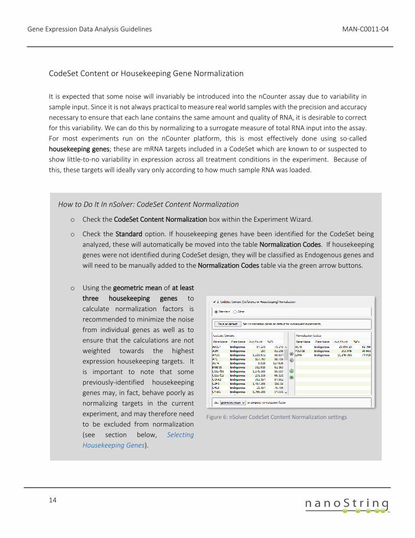
How to Do It In nSolver: CodeSet Content Normalization

o Check the CodeSet Content Normalization box within the Experiment Wizard.

o Check the Standard option. If housekeeping genes have been identified for the CodeSet being

analyzed, these will automatically be moved into the table Normalization Codes. If housekeeping

genes were not identified during CodeSet design, they will be classified as Endogenous genes and

will need to be manually added to the Normalization Codes table via the green arrow buttons.

o Using the geometric mean of at least

three housekeeping genes to

calculate normalization factors is

recommended to minimize the noise

from individual genes as well as to

ensure that the calculations are not

weighted towards the highest

expression housekeeping targets. It

is important to note that some

previously-identified housekeeping

genes may, in fact, behave poorly as

normalizing targets in the current

experiment, and may therefore need

to be excluded from normalization

(see section below, Selecting

Housekeeping Genes).

Figure 6: nSolver CodeSet Content Normalization settings


15

The calculations are performed automatically in nSolver, which follows this procedure (for an example of

this procedure, see the Positive Control Normalization section and Figure 5, above):

1. Calculate the geometric mean of the selected housekeeping genes for each lane.

2. Calculate the arithmetic mean of these geometric means for all sample lanes.

3. Divide this arithmetic mean by the geometric mean of each lane to generate a lane-specific

normalization factor.

4. Multiply the counts for every gene by its lane-specific normalization factor.


16

Normalization QC

It is important to perform some Quality Control on normalized nCounter data to ensure that normalization

has not inadvertently introduced variability into the data set. The scaling factors generated by Positive

Control and Housekeeping (CodeSet Content) Normalization can be used as surrogate measures for

potential bias which may be introduced by these procedures.

A Positive Control scaling factor for a sample that exceeds 3-fold (that is, it is less than 0.3 or greater than

3.0), may skew results from the samples, particularly for those low expression targets which are close to

the background noise. Scaling factors in these extreme ranges most commonly result from samples with

positive control counts that are much lower than normal. Even if these samples appear otherwise normal,

positive controls that are lower than expected may indicate a reduction in assay efficiency.

A CodeSet Content normalization scaling factor that exceeds 10-fold (less than 0.1 or greater than 10.0)

indicates that housekeeping genes have counts that are much lower than average for that sample. The

safest course would be to exclude samples with Normalization factors outside the expected range from

further analysis, although samples that yielded marginal QC specs (i.e., a ’12.0’ for CodeSet Content

Normalization) are often still usable. Even for samples with normalization flags, data from moderate- to

highly-expressed targets will often show little bias. More concerning are the data from low count targets;

these can become biased upwards for samples with normalization flags, and their inclusion may potentially

skew the results of a study. The use of background thresholding in nSolver will minimize this upward bias

in low count genes, but samples with normalization flags will still have a reduced ability to detect low

expression genes. See the Assessing QC Flags section to determine if these samples are outliers in the

normalized dataset.

Selecting Housekeeping Genes Not every pre-selected housekeeping gene will necessarily correlate well with sample input. Even well-validated housekeepers may show increased variability when tested under novel experimental conditions, new pathologies, or new tissue types. Therefore, it is good practice to critically examine the data from putative housekeeping genes and exclude any targets with notable instability in expression. Indications that you may need to discard a housekeeper include:

o A housekeeping target that is expressed at or near the background; this will likely introduce noise

into the normalized data.

o A housekeeping target with a higher variability than other targets (as measured by %CV; this

column can be seen in Figure 6 above, How to Do It In nSolver: CodeSet Content Normalization).

o A housekeeping target whose expression does not correlate with other housekeepers when

compared across samples. The nSolver Advanced Analysis module includes a published

methodology and algorithm (geNorm) to formally assess these characteristics and identify the

optimal housekeepers for the current data set. See the Advanced Analysis User Manual for more

information on optimizing normalization.


17

Assessing a Normalization QC Flag

o POS Control Flag: Samples with a POS Control Normalization flag have lower than typical POS control

counts, and may be experiencing a reduced level of assay level efficiency. These samples will also

sometimes receive an Assay Performance QC flag, due to factors such as: failed imaging QC, high

binding density, a failed pipetting step, or low hybridization efficiency, which should aid in determining

the root cause of the lowered efficiency. See the Assessing QC Flags section, above, to determine how

to treat these samples.

o Content (Housekeeping) Normalization Flag: Samples with a Content Normalization flag typically have

very low housekeeping gene counts, and thus likely have very low amounts of intact RNA. This may

result from pipetting errors, inaccurate quantification, or sample degradation. For help in determining

the root cause of low RNA counts, consult with NanoString support ([email protected]), but

also refer to the Assessing QC Flags section, above, to determine if the data from these samples should

still be included in further analyses.

How to Do It In nSolver: Normalization QC nSolver will automatically compare normalization factors for POS controls and Housekeeping genes to the default cutoffs mentioned in the text (3-fold and 10-fold, respectively). To determine whether samples received normalization flags:

o Select the Normalized Data table in the finished experiment (see Figure 7).

o Scroll right in the central table viewer: there are two columns reserved for potential normalization flags,

then two more for the normalization correction factors.

Figure 7: Normalization QC in nSolver



18

Ratios, Fold-Changes, and Differential Expression For many experiments that quantify mRNA expression levels, a primary end goal is to characterize changes in gene expression across samples that differ in some key characteristic (i.e., different pathology or treatment). Here, we describe the process of differential expression analysis in a NanoString gene expression dataset. We will also highlight important considerations in experimental design and how they may impact the ability to determine differential expression. An experiment that is designed to include biological replicates is amenable to formal statistical testing, as it maximizes biological inference of expression differences between sample groups. In contrast, experiments with one replicate per condition are limited in terms of both statistical testing options and biological interpretation. Technical replicates are not required, since the enzyme-free, digital nature of the assay generates exceptionally precise and reproducible measurements. Biological replicates, therefore, are strongly recommended. In the following sections, we discuss creating ratios and fold-change estimates, and for those experiments with sufficient biological replicates, we discuss appropriate statistical tests and multiple testing correction.

Ratio and Fold-Change Calculations Normalized NanoString gene expression data is most commonly analyzed in terms of ratios or fold-changes. These calculations are used to determine relative over- or under-expression of each gene across different sample groups in an experiment. These expressions can be calculated in either linear or log2 scale. Here, we illustrate how to calculate ratios using a hypothetical experiment with three groups of samples: those in a control group, those in group 1, and those in group 2. Calculating linear ratios for a single gene in this data set is shown in Figure 8. Overexpressed genes will have ratios >1, but under-expressed genes will have a ratio which ranges in value from 0 – 1 and are therefore compressed in the linear scale.

Comparison Linear Ratio Calculation Interpretation

Group #1 vs.

Control 𝑅𝑎𝑡𝑖𝑜 =

𝑔𝑒𝑜𝑚𝑒𝑡𝑟𝑖𝑐 𝑚𝑒𝑎𝑛 𝑜𝑓 𝑔𝑒𝑛𝑒 ‘A’ 𝑓𝑟𝑜𝑚 𝑔𝑟𝑜𝑢𝑝 #1

𝑔𝑒𝑜𝑚𝑒𝑡𝑟𝑖𝑐 𝑚𝑒𝑎𝑛 𝑜𝑓 𝑔𝑒𝑛𝑒 ‘A’ 𝑓𝑟𝑜𝑚 𝑐𝑜𝑛𝑡𝑟𝑜𝑙 𝑔𝑟𝑜𝑢𝑝

Relative over- or under-expression of

gene ‘A’ in group #1 vs. control

Group #2 vs.

Control 𝑅𝑎𝑡𝑖𝑜 =


𝑔𝑒𝑜𝑚𝑒𝑡𝑟𝑖𝑐 𝑚𝑒𝑎𝑛 𝑜𝑓 𝑔𝑒𝑛𝑒 ‘A’ 𝑓𝑟𝑜𝑚 𝑐𝑜𝑛𝑡𝑟𝑜𝑙 𝑔𝑟𝑜𝑢𝑝


gene ‘A’ in group #2 vs. control

Group #1 vs.

Group #2 𝑅𝑎𝑡𝑖𝑜 =




gene ‘A’ in group #1 vs. group #2

Figure 8: Linear ratio calculations


19

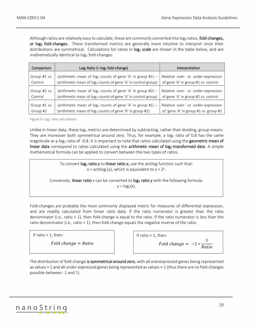
Although ratios are relatively easy to calculate, these are commonly converted into log2 ratios, fold-changes, or log2 fold-changes. These transformed metrics are generally more intuitive to interpret since their distributions are symmetrical. Calculations for ratios in log2 scale are shown in the table below, and are mathematically identical to log2 fold-changes.

Comparison Log2 Ratio (= log2 fold-change) Interpretation

Group #1 vs.

Control

(arithmetic mean of log2 counts of gene ‘A’ in group #1) –

(arithmetic mean of log2 counts of gene ‘A’ in control group)

Relative over- or under-expression

of gene ‘A’ in group #1 vs. control

Group #2 vs.

Control


(arithmetic mean of log2 counts of gene ‘A’ in control group)


of gene ‘A’ in group #2 vs. control

Group #1 vs.

Group #2


(arithmetic mean of log2 counts of gene ‘A’ in group #2)


of ‘gene ‘A’ in group #1 vs. group #2

Figure 9: Log2 ratio calculations

Unlike in linear data, these log2 metrics are determined by subtracting, rather than dividing, group means. They are moreover both symmetrical around zero. Thus, for example, a log2 ratio of 0.8 has the same magnitude as a log2 ratio of -0.8. It is important to note that ratios calculated using the geometric mean of linear data correspond to ratios calculated using the arithmetic mean of log2-transformed data. A simple mathematical formula can be applied to convert between the two types of ratios.

Fold-changes are probably the most commonly displayed metric for measures of differential expression, and are readily calculated from linear ratio data. If the ratio numerator is greater than the ratio denominator (i.e., ratio > 1), then fold-change is equal to the ratio. If the ratio numerator is less than the ratio denominator (i.e., ratio < 1), then fold-change equals the negative inverse of the ratio:

The distribution of fold-change is symmetrical around zero, with all overexpressed genes being represented as values > 1 and all under-expressed genes being represented as values <-1 (thus there are no fold-changes possible between -1 and 1).

If ratio > 1, then:

𝐹𝑜𝑙𝑑 𝑐ℎ𝑎𝑛𝑔𝑒 = 𝑅𝑎𝑡𝑖𝑜

If ratio < 1, then:

𝐹𝑜𝑙𝑑 𝑐ℎ𝑎𝑛𝑔𝑒 = −1 ∗1

𝑅𝑎𝑡𝑖𝑜

To convert log2 ratio y to linear ratio x, use the antilog function such that: x = antilog2(y), which is equivalent to x = 2y.

Conversely, linear ratio x can be converted to log2 ratio y with the following formula:

y = log2(x).


20

Statistical Tests In this section, we will cover a few basic recommendations for statistical testing of differential expression in nCounter data sets. It is beyond the scope of this document to exhaustively cover the various approaches that are appropriate for making statistical inferences from gene expression studies, so we will focus primarily on the options for testing which can be found in the nSolver analysis software. As stated previously, a minimum of three biological replicates are required from each experimental group to obtain reasonably reliable statistical information about the underlying populations from which those samples were drawn. If the magnitude of between-group differences is small, or if variability within groups is high, then more replicates per group may still be required to obtain statistical significance.

T-test A t-test can be performed on log2-transformed count data if there are only two groups of samples to compare. An example of this would be a simple experiment consisting of control group samples that you would like to compare to samples in a single treatment group. The log2 transformation will generally satisfy the t-test’s requirement of normally distributed data, and the use of a heteroscedastic t-test (Welch’s) also relaxes the assumption that variance is equally distributed among groups. The output of a t-test is a p-value, and standard convention is to assign significance to all genes with a nominal p-value of less than 0.05. The lower the p-value, the stronger the evidence that a gene has different expression levels in two different groups. It is important to note that a p-value is the probability of obtaining an effect at least as extreme as the one observed, assuming the null hypothesis of no difference between sample groups is true. The p-value addresses the question, “how likely is the data?”, assuming the null hypothesis is true. It is a common mistake for a specific p-value to be incorrectly interpreted as the probability of a false positive; this is called a Type I error. If desired, post-hoc corrections can be applied to adjust p-values to account for multiple testing (see below).

Multivariate Linear Regression Normalized and log2-transformed nCounter data may also be analyzed using multivariate linear regression. This is a powerful approach for dealing with more complex experimental designs than a two-group experiment. It allows one to isolate the independent effect of each covariate on gene expression levels, permitting comparisons between multiple experimental groups and variables, including potentially confounding variables. Though the details are beyond the scope of this document, guidance on how to perform these tests in the nSolver Advanced Analysis module may be found in the Advanced Analysis User Manual.


21

False Discovery Rate and Correcting for Multiple Comparisons In large, multiplexed gene expression datasets, the large number of statistical tests performed may inadvertently increase the chances of obtaining false-positive results. This is because, all else being equal, 1 out of every 20 statistical tests is expected by chance alone to result in a p-value of approximately 0.05, the traditional threshold for obtaining statistical significance. The frequency of these potential false positives is expected to go up with increasing numbers of tested genes, so for larger NanoString CodeSets, this may become a potential concern.

Despite this possibility, we do not necessarily recommend a universal application of multiple comparison corrections for NanoString datasets. First, CodeSets generally comprise collections of genes known or suspected to be affected by the biology under study, and the resulting correlations in expression levels violates the assumption of independence of significance levels between tests, which forms the basis of the more conservative Bonferroni multiple comparisons tests.

As a corollary, if the purpose of the NanoString study is to validate the results of a transcriptome-wide survey, the CodeSet will, just as above, comprise a highly non-random set of genes. For such validation work, it may not be desirable at this stage to limit the number of false positives. Arguably, instead of statistical adjustments to significance levels, one might consider cross-platform validation as a better standard towards determining the statistical robustness of any expression level differences.

Lastly, the use of multiple comparisons corrections may simply be too conservative for experiments where the tolerance for false negatives is low. Statistical methods designed to reduce the number of false positives will invariably result in an increase in the number of false negatives, and for some experimental goals, this extra level of stringency may not be an acceptable tradeoff.

In general, when multiple comparison corrections are performed on NanoString data, using a less conservative method which allows gene significance levels to be either positively or negatively correlated is preferred (i.e., when probing for correlated and interdependent expression pathways). The Benjamini-Yekutieli False Discovery Rate method1 accounts for this expectation that significant changes in genes may be correlated with or dependent on each other, and the resulting FDR adjusted p-value provides a middle ground between the more conservative tests which control for family-wise error rates (epitomized by tests like the Bonferroni correction) and more permissive uncorrected p-values.

1 The Benjamini-Yekutieli adjustment was originally described in the following publication: Benjamini, Y, and Yekutieli, D. (2001) "The control of the false discovery rate in multiple testing under dependency." Annals of Statistics. 29(4):1165-1188.


22

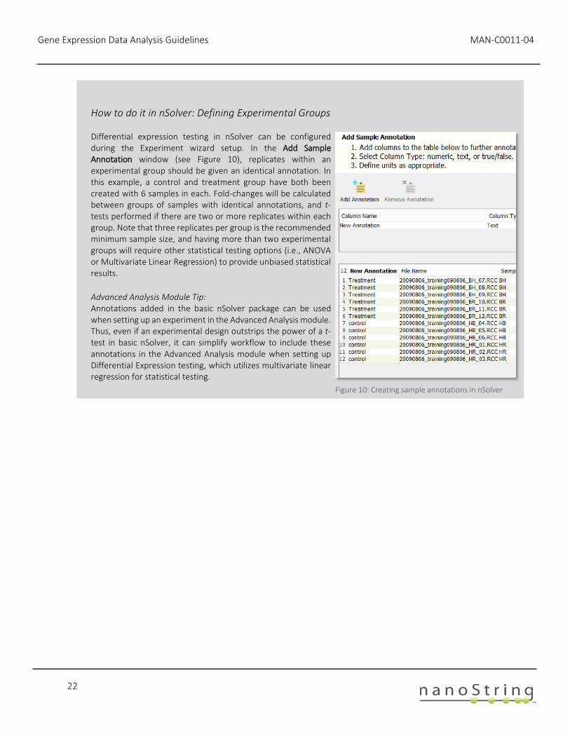
How to do it in nSolver: Defining Experimental Groups

Differential expression testing in nSolver can be configured during the Experiment wizard setup. In the Add Sample Annotation window (see Figure 10), replicates within an experimental group should be given an identical annotation. In this example, a control and treatment group have both been created with 6 samples in each. Fold-changes will be calculated between groups of samples with identical annotations, and t-tests performed if there are two or more replicates within each group. Note that three replicates per group is the recommended minimum sample size, and having more than two experimental groups will require other statistical testing options (i.e., ANOVA or Multivariate Linear Regression) to provide unbiased statistical results. Advanced Analysis Module Tip: Annotations added in the basic nSolver package can be used when setting up an experiment in the Advanced Analysis module. Thus, even if an experimental design outstrips the power of a t-test in basic nSolver, it can simplify workflow to include these annotations in the Advanced Analysis module when setting up Differential Expression testing, which utilizes multivariate linear regression for statistical testing.

Figure 10: Creating sample annotations in nSolver


23

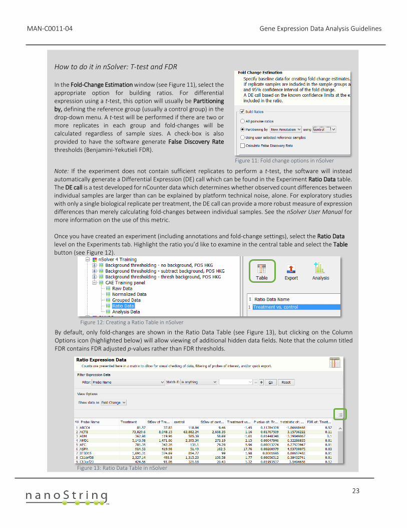
How to do it in nSolver: T-test and FDR In the Fold-Change Estimation window (see Figure 11), select the appropriate option for building ratios. For differential expression using a t-test, this option will usually be Partitioning by, defining the reference group (usually a control group) in the drop-down menu. A t-test will be performed if there are two or more replicates in each group and fold-changes will be calculated regardless of sample sizes. A check-box is also provided to have the software generate False Discovery Rate thresholds (Benjamini-Yekutieli FDR).

Note: If the experiment does not contain sufficient replicates to perform a t-test, the software will instead automatically generate a Differential Expression (DE) call which can be found in the Experiment Ratio Data table. The DE call is a test developed for nCounter data which determines whether observed count differences between individual samples are larger than can be explained by platform technical noise, alone. For exploratory studies with only a single biological replicate per treatment, the DE call can provide a more robust measure of expression differences than merely calculating fold-changes between individual samples. See the nSolver User Manual for more information on the use of this metric. Once you have created an experiment (including annotations and fold-change settings), select the Ratio Data level on the Experiments tab. Highlight the ratio you’d like to examine in the central table and select the Table button (see Figure 12).

By default, only fold-changes are shown in the Ratio Data Table (see Figure 13), but clicking on the Column Options icon (highlighted below) will allow viewing of additional hidden data fields. Note that the column titled FDR contains FDR adjusted p-values rather than FDR thresholds.

Figure 11: Fold change options in nSolver

Figure 12: Creating a Ratio Table in nSolver

Figure 13: Ratio Data Table in nSolver