gene-environment case-control studies raymond j. carroll department of statistics faculties of...

Gene-Environment Case-Control Studies

Raymond J. CarrollDepartment of StatisticsFaculties of Nutrition and

Toxicology

Texas A&M Universityhttp://stat.tamu.edu/~carroll

Outline

• Problem: Case-Control Studies with Gene-Environment relationships

• Efficient formulation when genes are observed

• Measurement errors in environmental variables

• Haplotype modeling and Robustness

Acknowledgment

• This work is joint with Nilanjan Chatterjee (NCI) and Yi-Hau Chen (Academia Sinica)

Acknowledgment

• Further work is joint with Mitchell Gail (NCI), Iryna Lobach (Yale) and Bhramar Mukherjee (Michigan)

Software

• SAS and Matlab Programs Available at my web site under the software button

• Examples are given in the programs

http://stat.tamu.edu/~carroll

Some Personal History

• I was born in Japan

• The coffee table is still in my house

Some Personal History

• My father lived in Seoul for 2 months in 1948 and 1 year in 1968

• He took many photos of sights there, especially in 1948

Joonghwa moon at Deoksugung, 1948

Joonghwa moon at Deoksugung, today

The Prices of Drinks Were Pretty Low

Basic Problem Formalized

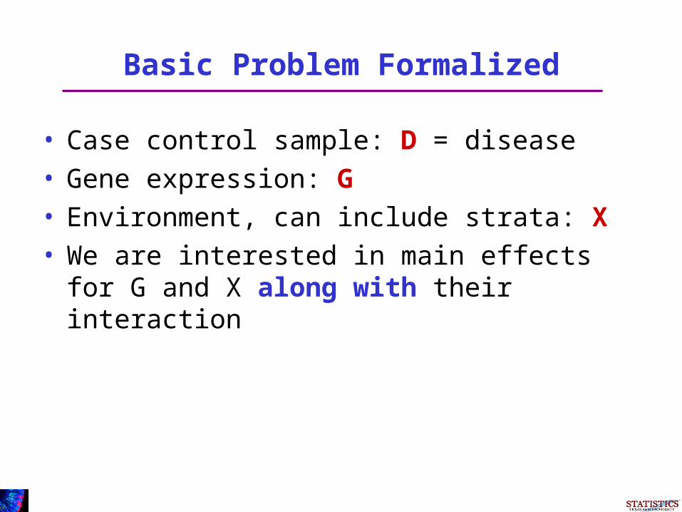
• Case control sample: D = disease • Gene expression: G• Environment, can include strata: X• We are interested in main effects for G

and X along with their interaction

Prospective Models

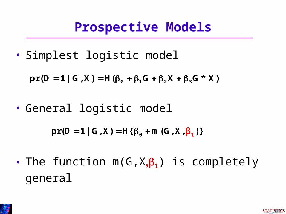
• Simplest logistic model

• General logistic model

• The function m(G,X1) is completely

general

0 1 2 3pr(D 1| G,X) H( G X G* X)

0 1pr(D 1| G,X) H{ m(G,X, )β }

Likelihood Function

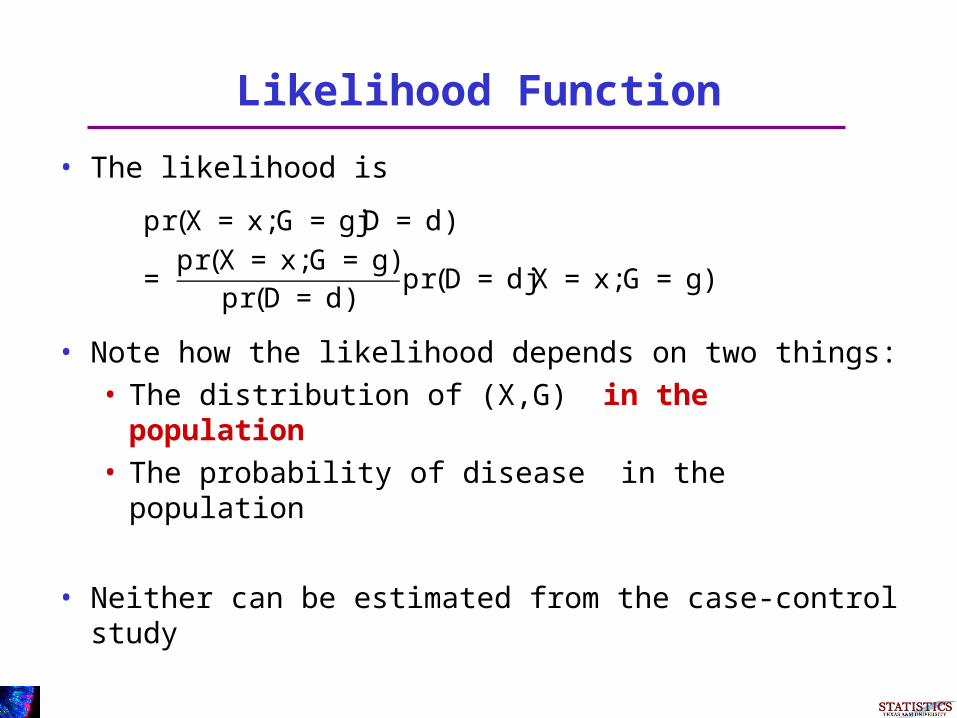
• The likelihood is

• Note how the likelihood depends on two things:• The distribution of (X,G) in the population• The probability of disease in the population

• Neither can be estimated from the case-control study

pr(X = x;G = gjD = d)

=pr(X = x;G = g)

pr(D = d)pr(D = djX = x;G = g)

When G is observed

• The usual choice is ordinary logistic regression

• It is semiparametric efficient if nothing is known about the distribution of G, X in the population

• Why semiparametric: what is unknown is the distribution of (G,X) in the population

When G is observed

• Logistic regression is thus robust to any modeling assumptions about the covariates in the population

• Unfortunately it is not very efficient for understanding interactions

Gene-Environment Independence

• In many situations, it may be reasonable to assume G and X are independently distributed in the underlying population, possibly after conditioning on strata

• This assumption is often used in gene-environment interaction studies

G-E Independence

• Does not always hold!

• Example: polymorphisms in the smoking metabolism pathway may affect the degree of addiction

• Part of this talk is to model the distribution of G given X

Gene-Environment Independence

• If you’re willing to make assumptions about the distributions of the covariates in the population, more efficiency can be obtained.

• The reason is that you are putting a constraint on the retrospective likelihood

pr(X = x;G = gjD = d)

=pr(X = x;G = g)


More Efficiency, G Observed

• A constraint on the population is to posit a parametric or semiparametric model for G given X

• Consequences: • More efficient estimation of G effects• Much more efficient estimation of G and (X,S)

interactions.

pr(G g| X) q(g θ| X, )

The Formulation

• In the most general semiparametric setting, we have

• Question: What methods do we have to construct estimators?

10pr(D 1| G,X) H β m(G,X, ) ,

pr(G g| X) q(g| X, )

X Nonparametric,multi dimension

β

a

θ

l

Methodology

• We have developed two new ways of thinking about this problem

• In ordinary logistic regression case-control studies, they reduce to the Prentice-Pyke formulation

The Hard Way

• Treat X as a discrete random variable whose mass points are the observed data points

• Holding all parameters fixed, maximize the retrospective likelihood to estimate the probabilities of the X values.

=q(gjX ;µ) pr(X = x)


The Hard Way

• The maximization is not trivial to do correctly

• Result: an explicit profile likelihood that does not involve the distribution of X

Pretend Missing Data Formulation

• The following simple trick can be shown to be legitimate and semiparametric efficient

• Equivalently, we compute a semiparametric profiled likelihood

• Semiparametric because the distribution of X is not modeled


• The idea is to create a “pretend” study, which is one of random sampling with missing data

• We use an MAR regime.

• The “pretend” study mimics the case-control study


• Suppose you have a large but finite population of size N

• Then, there are with the disease

• There are without the disease

N¼1

N¼0


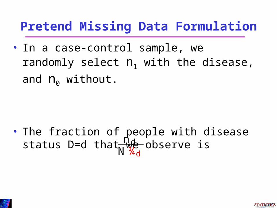
• In a case-control sample, we randomly select n1 with the disease, and n0 without.

• The fraction of people with disease status D=d that we observe is

ndN ¼d


• Then let’s make up a “pretend” study, that has random sampling with missing data

• I take a random sample• I get to observe (D,X,G) when D=d with

probability

• I will say that if I observe (D,X,G). Then

ndN ¼d

±= 1

pr(±= 1jD = d;X ) = pr(±= 1jD = d) = ndN ¼d


• In this pretend missing data formulation, ordinary logistic regression is simply

• We have a model for G given X, hence we compute

• This has a simple explicit form, as follows

G=gpr(D=d| , =1,X)

G=gpr(D=d, | =1,X)

Result

• Define

• This is the intercept that ordinary logistic regression actually estimates– It only gets the slope right

¯ ¤0 = ¯ 0 + log(n1=n0) ¡ log(¼1=¼0)

Result

• Define

•

• Further define

S(d;x;g;£ ) =q(g;µ)exp [d f¯ ¤

0 + m(x;g;¯ 1)g]1+ exp f¯ 0 + m(x;g;¯ 1)g

£ = (¯ 0;¯ 1;µ;¯ ¤0) = (¯ 0;¯ 1;µ;¼1)

¯ ¤0 = ¯ 0 + log(n1=n0) ¡ log(¼1=¼0)

Result

• Then, the semiparametric efficient profiled likelihood function is

• Trivial to compute.

S(d;x;g;£ ) =q(g;µ)exp [d f¯ ¤

0 + m(x;g;¯ 1)g]1+ exp f¯ 0 + m(x;g;¯ 1)g

L semi(X ;GjD;£ ) =S(D;X ;G;£ )

P 1d=0

P 1s=0 S(d;X ;s;£ )

Result

• In the rare disease case, we have the further simplification that

S(d;x;g;£ ) = q(g;µ)exp [d f ¯ ¤0 + m(x;g;¯ 1)g]

L semi(X ;GjD;£ ) =S(D;X ;G;£ )

P 1d=0

P 1s=0 S(d;X ;s;£ )

Interesting Technical Point

• Profile pseudo-likelihood acts like a likelihood

• Information Asymptotics are (almost) exact

L semi(X ;GjD;£ )

Typical Simulation Example

• MSE Efficiency of Profile method compared to ordinary logistic regression

0

0.5

1

1.5

2

2.5

3

3.5

4

G X G times X

pr(G)=.05

pr(G)=.20

Typical Empirical Example

Consequence #1

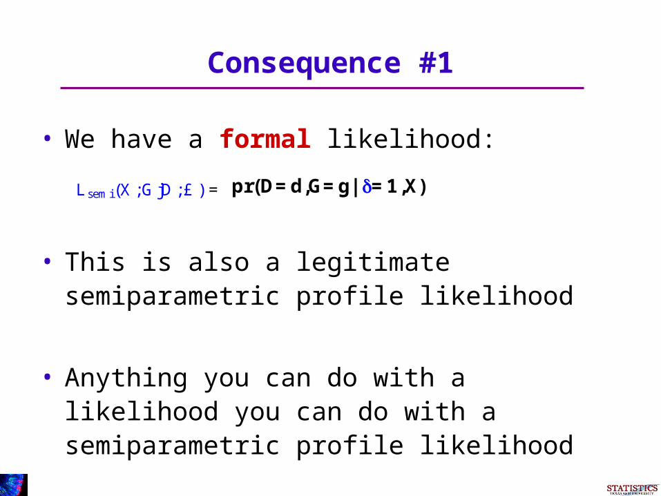
• We have a formal likelihood:

• This is also a legitimate semiparametric profile likelihood

• Anything you can do with a likelihood you can do with a semiparametric profile likelihood

pr(D=d,G=g| =1,X)L semi(X ;GjD;£ ) =

Consequences #2-#3

• Measurement Error in the Gene:• Handle misclassification of a covariate (the

gene) as in any likelihood problem (see later)

• Measurement Error in the Environment :• The structural approach, wherein you specify a

flexible model for covariates measured with error, is applicable.

Advertisement

Lobach, et al., Biometrics, in press

Consequences #4-#5

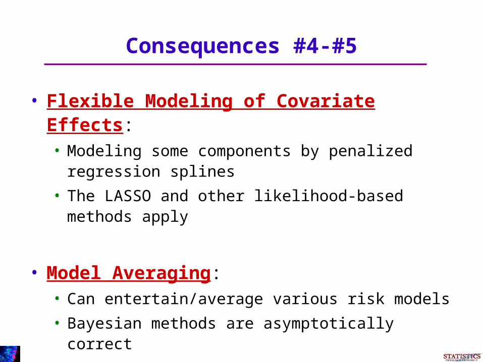
• Flexible Modeling of Covariate Effects:• Modeling some components by penalized

regression splines

• The LASSO and other likelihood-based methods apply

• Model Averaging:• Can entertain/average various risk models

• Bayesian methods are asymptotically correct

Consequence #6

• Model Robustness:• One can model average/select/LASSO various

models for the distribution of G given X

• Main Point: Our method results in a legitimate likelihood, hence can be treated as such

Modeling the Gene

• Now turn to models for the gene

• Given such models likelihood calculations can be used for model fitting

• We will consider haplotypes

Haplotypes

• Haplotypes consist of what we get from our mother and father at more than one site

• Mother gives us the haplotype hm = (Am,Bm)

• Father gives us the haplotype hf = (af,bf)

• Our diplotype is Hdip = {(Am,Bm), (af,bf)}

Haplotypes

• Unfortunately, we cannot presently observe the two haplotypes

• We can only observe genotypes

• Thus, if we were really Hdip = {(Am,Bm), (af,bf)}, then the data we would see would simply be the unordered set (A,a,B,b)

Missing Haplotypes

• Thus, if we were really Hdip = {(Am,Bm), (af,bf)}, then the data we would see would simply be the unordered set (A,a,B,b)

• However, this is also consistent with a different diplotype, namely Hdip = {(am,Bm), (Af,bf)}

• Note that the number of copies of the (a,b) haplotype differs in these two cases

• The true diploid = haplotype pair is missing

Missing Haplotypes

• The likelihood in terms of the diploid is

• We observe the genotypes G

• The likelihood of the observed data is

L semi(X ;H dipjD;£ )

X

hdip 2G

L semi(X ;hdipjD;£ )

Missing Haplotypes

• The likelihood of the observed data is

• Note how easy this was: it is really the profiled semiparametric likelihood of the observed data

X

hdip 2G

L semi(X ;hdipjD;£ )

Haplotypes

• Danyu Lin has a nice EM-based program for estimating haplotype frequencies

• It accepts data in text format with SAS missing data conventions

• The program is flexible, and for example it can assume Hardy-Weinberg equilibrium (HWE)

http://www.bios.unc.edu/~lin/hapstat/




Haplotype Fitting

• Models that assume haplotype-environment independence are straightforward to fit via EM• Danyu Lin’s program can do this as well as our

SAS program

• The remaining issue is how to gain robustness against deviations from this assumed independence

Robustness

• We build robustness by specifying models for diplotypes given the environmental variables

• We first run a program to get a preliminary estimate of haplotype frequency

• We use the most frequent haplotype as a reference haplotype

Haplotypes

• Approach: Start with a logistic model for the unobserved haplotypes H given covariates X

• In practice, we collapse all rare haplotypes into the reference haplotype to eliminate many variables

j k

0jk 1jk

ref ref

dip

dip

pr H =(h ,h )| Xlog X

pr H =(h ,h )| X

Haplotypes

• Approach: Start with a logistic model for the unobserved haplotypes H given covariates X

• This gives us the model:

j k

0jk 1jk

ref ref

dip

dip

pr H =(h ,h )| Xlog X

pr H =(h ,h )| X

hapdip dip d

0 1ippr(H h | X) q (h | X, , )

Haplotypes

• Since the diplotypes are not observed, for identifiability we need further constraints

• Example: One simple additive-type model is that

hapdip dip d

0 1ippr(H h | X) q (h | X, , )

1jk j k

Haplotypes

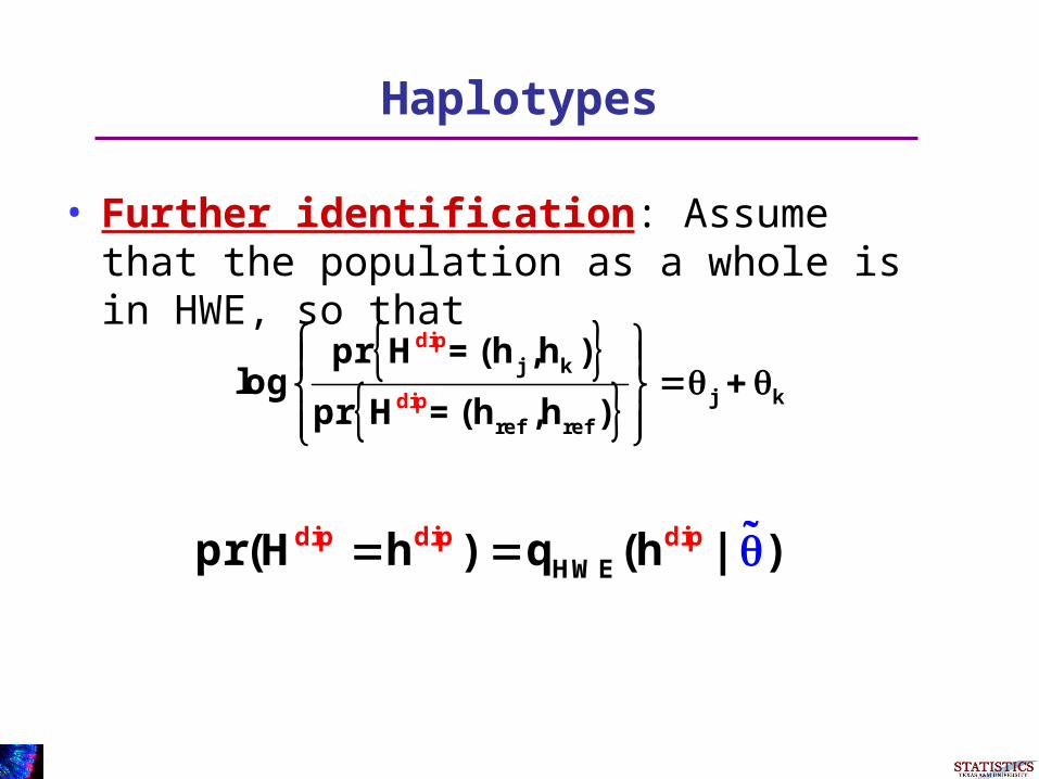
• Further identification: Assume that the population as a whole is in HWE, so that

j k

j k

r

dip

def re

ipf

pr H =(h ,h )log

pr H =(h ,h )

HWEdip dip dippr(H h ) q (h | )

Haplotypes

• Summary: We have two models


hapdip dip d

0 1ippr(H h | X) q (h | X, , )

Haplotypes

• Summary: The models are linked

• Let F(x) be the marginal distribution of X Then

dip dipHW h p 0 1E aq (h | ) q (h | x, , ) Fd (x)

Haplotypes

• In this set up, we have • a particular form for

• a particular form for

• hence is defined through them and the marginal distribution of X


0

1

Marginal Distributions of X

• Three approaches for estimating F(x)• Profiled likelihood

• If pr(D=1) is known, weighted mixture of empirical cdf for cases and controls

• For rare disease, the empirical cdf for the controls


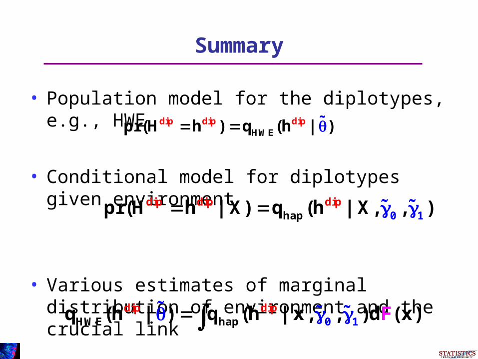
Summary

• Population model for the diplotypes, e.g., HWE

• Conditional model for diplotypes given environment

• Various estimates of marginal distribution of environment and the crucial link


hapdip dip d

0 1ippr(H h | X) q (h | X, , )


Haplotypes Analysis

• The resulting method adds robustness

• EM-algorithms enable fast computation

• Explicit asymptotic theory (not trivial)

• The method is also semiparametric efficient

Haplotypes Analysis

• Simulations indicate the gain in robustness

The NAT2 Example

• Study of colorectal adenoma, a precursor to colon cancer

• 628 cases and 635 controls• The gene NAT2 is known to be important

in the metabolism of smoking-related carcinogens

• X: age, gender, whether one smokes or used to smoke

• 6 SNPS• Haplotype 101010 is of interest

The NAT2 Example

• 7 Haplotypes had frequency > 0.5%

• The most frequent was treated as baseline, additive risk model for the diplotypes

• Interactions of smoking variable with the haplotype 101010 in the risk model

• Interactions of the smoking variable with the haplotypes in the gene model

The NAT2 Example

• Current smoking and 101010 haplotype interaction

Estimate

s.e. P-value

Independence

-0.29 0.18 0.109

Dependence -0.56 0.27 0.039

The NAT2 Example

• In this example, recognizing the possibility that the gene distribution may depend on the environment (smoking) changes the analysis

• Plus, we get a p-value < 0.05!

Further work

• These is another way to get robustness that we have just submitted

• The idea is that the haplotypes and the environment are independent given the genotypes

• That is, once you know the genotypes, the haplotypes are determined solely by random mating.

Further work

• We then have two estimates:• Haplotype-environment unconditional

independence• Independence conditional on the genotype

• Then we do a penalized likelihood analysis– Likelihood is the conditional independence

likelihood– The penalty is the L1 distance from the

unconditional independence estimate

Further work

• The result is increased robustness and major gains in efficiency

Summary

• Fully flexible risk models

• Flexible models for genes/haplotypes given covariates

• Computable semiparametric efficient inference that is more powerful than ordinary logistic regression and more robust than gene-environment independence

Thanks!

http://stat.tamu.edu/~carroll

gene-environment case-control studies raymond j. carroll department of statistics faculties of...

Documents