Gender Bias in the Enforcement of Traffic Laws:

Evidence based on a new empirical test∗

Brian Rowe†

Bureau of EconomicsFederal Trade Commission

browe@ftc.gov

September 2009

Abstract

In the United States, a majority of the drivers who receive a traffic ticket are male, and maledrivers are more likely to receive a ticket after being stopped by the police. This paper developsand conducts an empirical test for the existence of police gender bias (taste-based discrimination)in traffic ticketing. The test is based on a model’s prediction of how the gender compositionof ticketed drivers should vary across groups of police officers who use unbiased, but potentiallydifferent ticketing standards. The test is useful for determining whether the gender disparity intraffic tickets results from gender bias or a higher tendency of male drivers to break traffic laws. Inaddition, the test offers an improvement over the “differences-in-differences” test for discriminationwhich has been applied in other contexts. When applied to data on traffic tickets issued by maleand female police officers in Boston, the new test rejects the null hypothesis of unbiased ticketing.

JEL Codes: J16, J71, K42∗I am grateful to Martha Bailey, Alexia Brunet, Osborne Jackson, Zoe McLaren, Matt Rutledge, J.J. Prescott,

Dan Silverman, Jeff Smith, seminar participants at the University of Michigan, the Midwest Economic Association’s2008 meeting, the American Law and Economics Association’s 2008 meeting, and the Conference on Empirical LegalStudies 2008 meeting for many helpful comments. I thank Kate Antonovics, Bill Dedman, and Nicola Persico forsharing data.

†The views expressed in this article are those of the author and do not necessarily reflect those of the FederalTrade Commission.

1

1 Introduction

Traffic enforcement in the United States imposes a disparate impact on male drivers. In 2005,63.4% of all traffic tickets in the U.S. were issued to males.1 Furthermore, the gender disparity intickets is in excess of the male share of the driving population. In 2005, 10.8 percent of all maledrivers but only 6.8 percent of female drivers were stopped by police, and after being stopped maleswere more likely to be ticketed (Durose et al. 2007).

Traffic accidents are a significant public health problem in the United States.2 Because ofthis, road safety would be viewed as a legitimate law enforcement objective by the courts. In theU.S., police practices which impose a disparate impact on a demographic group are often (but notalways) upheld by the courts if the disparate impact is a byproduct of a legitimate law enforcementobjective. On the other hand, police practices which seem based on prejudice or are unrelated toeffective law enforcement are not permitted.3

In this way, the framework for determining the legality of police practices accords well withthe distinction between statistical and taste-based discrimination (bias) in economics. Statisticaldiscrimination can produce disparate impacts which are due to a legitimate objective and may bepermissible. Similarly, omitted variables related to criminality and correlated with race or gendercan produce disparate impacts even if the police are concerned only with effective law enforcement.This paper develops and conducts an empirical test for police gender bias in traffic enforcement.

It is difficult to determine empirically if the disparate impact of a police practice is at leastpartly due to bias. To solve this problem in the context of traffic enforcement, I develop a modelof police preferences and driver behavior which provides a testable implication of gender biasedticketing. The testable implication is in terms of what I call the “officer gender effect”: Conditionalon breaking a traffic law, does the probability that a female driver receives a ticket depend on thegender of the officer who observes the violation? The model serves to clarify the conditions whichare required to infer that a bias exists if this officer gender effect is found empirically.

In the model, the police receive a greater benefit from ticketing more dangerous traffic violations.In this way, the model provides an underlying motivation for traffic ticketing which is connected tothe objective of safety on the roads. Officers incur a cost from ticketing a driver, and the cost ofticketing is allowed to vary with both the gender of the police officer and the gender of the driver.The ticketing costs reflect a taste for discrimination. If an officer’s cost of ticketing male drivers islower than his cost of ticketing females, then all else equal the officer will derive more utility from

1According to Durose et al. (2007) in a Bureau of Justice Statistics special report, 11 million male drivers and 6.9million female drivers were stopped by police nationwide in 2005. 59.2% of the stopped male drivers were ticketedwhile 54.4% of the female drivers received a ticket. These figures imply that about 63.4% of all traffic tickets wereissued to male drivers.

2Approximately 42,000 people were killed and 2.5 million people were injured in traffic accidents in 2006 (2006Annual Assessment of Motor Vehicle Crashes, National Highway Traffic Safety Administration).

3See Knowles, Persico, and Todd (2001) for a more thorough discussion of the relevant legal background. Theconcept of an “unjustified disparate impact” is discussed in detail by Ayres (2002).

2

ticketing males. As the cost of ticketing male drivers increases, the officer increases his violationthreshold for males, which is the least dangerous traffic violation for which he is willing to ticket amale driver.

The test for gender bias is based on the model’s prediction for what the sign of the officer gendereffect should be if male and female police use unbiased (equal for each driver gender) but differentviolation thresholds. In this case, the officer gender using the higher threshold will be relativelymore likely to ticket male drivers who commit violations. This prediction depends on assumingthat male drivers are more dangerous, in that they are more likely to commit a traffic violation ofseverity level above a given threshold. I show that this assumption is supported by several patternsin the Boston data, as well as by findings from other research.4 Intuitively, relatively fewer femaledrivers commit violations which are dangerous enough to exceed a high threshold.

Estimating the officer gender effect is a difficult exercise because only drivers who receivedtickets appear in the data, so it is impossible to condition on breaking the law. If male and femaleofficers observed the same pool of drivers who broke the law, the officer gender effect is identifiedsimply as the empirical effect of the police officer being male on the probability that a ticketeddriver is female. In practice, male and female officers might monitor different areas of the city ortend to patrol at different times, and thereby observe different pools of drivers. To correct for thisI use an extensive set of traffic stop level controls to account for any variation in the pool of driversby observable characteristics such as time of day, day of week, and location in the city of Boston. Ifmale and female officers observe the same pool of drivers after conditioning on this information, theempirical effect of the officer being male on the probability that a ticketed driver is female equalsthe officer gender effect. This follows from logic similar to that of Grogger and Ridgeway (2006).I examine the validity of this strategy by looking at a variety of evidence in the traffic ticket dataand from some external sources.

To rank male and female officer’s violation thresholds, I estimate how the miles-per-hour overthe limit or dollar fine amount of ticketed violations depends on the gender of the police officer. Ishow that this method is valid if the rank order of average miles-per-hour preserves the rank orderof average violation severity, and if on average male drivers commit violations which are at least asdangerous as those committed by females.5

When applied to data on traffic tickets issued in Boston, my test rejects the null hypothesisof no gender bias in favor of the alternative that at least one officer gender is biased. First, maleofficers were less likely than female officers to ticket female drivers. I find no evidence that thiseffect is due to differences in the pools of drivers observed, so I infer that male officers were lesslikely to ticket female drivers who broke the law. Second, male officers were “tougher” because

4For example, Levitt and Porter (2001) find that the two-car fatal crash risk for male drivers is 3 times higherthan that of female drivers.

5As will be explained in Section 2, the model actually suggests several ways of ranking violation thresholds. Allof these produce the same ranking.

3

they issued tickets for relatively less dangerous violations (lower miles-per-hour and fine amounts).According to the test, this pattern could not be observed if both officer genders were unbiased.If there was no bias, male police officers should have been more likely to ticket female drivers byvirtue of being tougher (using a lower threshold).

Using the empirical results and some additional assumptions, I estimate the quantitative impactof the gender bias. In particular, I assume that driver behavior would not respond to the changes inviolation thresholds which provide the thought experiment for a back of the envelope calculation.Supposing male police are biased while female police are not, my calculation implies that 1,902tickets (1.3 percent of the total), would need to be re-allocated from male to female drivers tocorrect the gender bias. Alternatively, if female police are biased while male police are not, asimilar calculation implies that only 136 tickets should be re-allocated to males from females.

After an article in the Boston Globe documented sizable racial and gender disparities in traffictickets (Dedman and Latour 2003), the state of Massachusetts sponsored a follow-up study.6 Thisstudy finds that males were ticketed in excess of a benchmark population, such as the share ofmales in the local driving population, throughout Massachusetts (Farrell et al. 2004). Perhapsin response to these findings, the Boston Police Department acted to limit police discretion inticketing (Dedman 2004). My back of the envelope calculations suggest that at least with respectto gender, most of the disparity in tickets in Boston seems to result from gender differences indriving behavior.

Many studies of discrimination estimate how an outcome for subjects of a given racial or gendergroup depends on the racial or gender group of the evaluators who decide the outcome.7 Thisis done by including the interaction of subject and evaluator race or gender in the model for theoutcome. The idea underlying the estimation of these “cross-gender” or “cross-race” effects (whichare difference-in-differences estimates, as shown in the Appendix) is that any dependence of theoutcome on the subject-evaluator pairing of groups is difficult to reconcile as resulting from animportant omitted variable or statistical discrimination. It remains difficult, however, to determinewhether a cross effect implies bias. My analysis shows that cross effects can be generated whenevaluators are unbiased but use different standards, and my test is one potential solution to theproblem of drawing an inference about bias based on the estimation of a cross effect.

1.1 Recent Related Literature

Makowsky and Stratmann (2009), Blalock et al. (2007), and Rowe (2009) find that male driversin Massachusetts are more likely to receive a ticket after being stopped by the police, even after

6The article gives the example of a 23 year old female college student who was pulled over four times in a threeweek period and never received a ticket. In the data used in this paper, containing records of all traffic citations inBoston from April 2001 to January 2003, male drivers received 71% of the citations.

7Recent examples include Antonovics and Knight (2009), Bagues and Esteve-Volart (2007), Price and Wolfers(2007), and Schanzenbach (2005).

4

accounting for many relevant controls. These results only confirm that in the benchmark populationof stopped drivers, males are more likely to be ticketed.

Bagues and Esteve-Volart (2007) find that female candidates are more likely to pass the publicexamination for a position with the Corps of the Spanish Judiciary when the share of males on theevaluation committee is larger. They argue that this cross-gender effect suggests that committeesare gender biased. Price and Wolfers (2007) find that black basketball players have more foulscalled against them when the referees are white. They conclude that racial bias is the most plausibleexplanation for this cross-race effect after systematically ruling out several alternative explanations.My test offers an additional approach for interpreting the cross effects in these two studies, whichI discuss in Section 4.

Broadly speaking, the literature on testing for racial bias in motor vehicle searches attempts tosolve two critical problems which arise in the searches context.8 First, omitted variables which arecorrelated with driver race could lead to incorrect findings of bias. Second, the researcher is unableto identify the least suspicious drivers who the police found worthy of searching (the marginalmotorists). In the context of testing for bias in traffic ticketing, analogous problems appear, andmy test is a potential solution. The model I develop allows for unobserved violation severity toaffect officer’s decisions, and the test does not require knowledge of the marginal violator.

The test I develop exploits a situation in which male and female police are unbiased yet havedifferent costs of ticketing, and therefore use different thresholds. If police of different racial groupshave different costs of search on average (i.e., one racial group of officers is more likely to search allracial groups of drivers), the test developed by Anwar and Fang (2006) has zero power to detectrelative racial bias.9 My test is able to detect relative gender bias (one group is more biased thanthe other) when officer’s ticketing costs are different.

While my test exploits a difference in ticketing costs, the test developed by Antonovics andKnight (2009) requires the researcher to control for average differences in search costs by officerrace. Also, their test requires conditioning on a qualified pool of drivers who are at risk of a search.In Section 4, I conduct tests for gender bias in ticketing which are analogous to those of Anwarand Fang (2006) and Antonovics and Knight (2009). These tests produce different results than mytest, and I examine the reasons why.

8Knowles, Persico, and Todd (2001) developed the “hit rate” test for racial bias in searches of stopped motoristsfor drugs. Dharmapala and Ross (2004) analyze the hit rate test when some fraction of motorists always carry drugs.Anwar and Fang (2006) develop a test for relative racial prejudice based on ranking search rates and hit rates byofficer race. Antonovics and Knight (2009) construct a test based on officer heterogeneity and the mismatch of officerand driver race.

9Anwar and Fang (2006) explain this in footnote 35 of their paper.

5

2 The Model

This model explains why the police choose to ticket some drivers who break the law but not others,which is a new application for a model of police behavior. After developing the model, I derive atestable implication of gender biased traffic ticketing.

2.1 Model set-up

The police patrol the roads and observe traffic violations committed by drivers, such as running ared light, driving faster than the speed limit, or changing lanes without signaling. The police havefull knowledge of traffic laws and they know with certainty when a traffic law has been violated.A key aspect of traffic law enforcement is police discretion, because many observed violations arenot ticketed. For example, according to the 2005 Police-Public Contact Survey, only 57.4% of allstopped drivers received a ticket (Durose et al. 2007). Also, from April to May of 2001, only 49percent of Boston drivers who were stopped (and received written documentation) received a ticketas opposed to a warning. This model assumes that police discretion in ticketing operates by officersevaluating the severity, or the danger imposed on others, of the traffic violations they observe.10

The police officer observes the severity, θ ∈ (0,∞), of each traffic violation, but θ is not observedby the researcher. The severity or danger level of a traffic violation depends on the speed of themotorist, the amount of traffic, the weather and road conditions, the presence of pedestrians, andother factors which may not be observed. All of this relevant information is summarized by θ.Police receive a benefit b(θ) from ticketing a violation of severity θ, with ∂b(θ)

∂θ > 0 because officersare concerned about public safety. By ticketing a violator, officers incur a cost t(dg, pg), which isallowed to depend on both the gender g ∈ {m, f} of the driver dg and the gender of the police officerpg. Officers incur this cost because issuing a ticket requires labor effort in the form of stopping thedriver, checking his license and registration, and dealing with any objections raised by the driver.

Definition of Bias. A police officer of gender pg is biased if t(dm, pg) 6= t(df , pg).

This defines bias as taste-based discrimination, as originally described by Becker (1957). Forinstance, if an officer’s cost of ticketing males is lower, for equally dangerous violations the officerwill derive more utility from ticketing males. Since the utility from not giving a ticket is zero,officers use the following decision rule:

Ticketing Rule. Officers ticket an observed violation if b(θ)− t(dg, pg) ≥ 0.

The ticketing rule generates the following result:10Rowe (2009) offers a rationalization for the existence of warnings (where the stopped driver receives no fine) in

an efficient enforcement scheme, based on the idea that traffic stops act to detect other crimes. The model he usesdoes not explain how the police choose which stopped drivers to ticket. However, in that setting more dangerousoffenses should be ticketed with a higher probability. This is consistent with the model developed here, which doesexplain officer’s choices of warnings versus tickets.

6

Proposition 1. Police officers ticket an observed violation only if θ ≥ θ∗(dg, pg), where the thresh-old violation θ∗(dg, pg) is determined by b(θ∗) = t(dg, pg). The threshold θ∗(dg, pg) increases mono-tonically as the ticketing cost t(dg, pg) increases.

Proposition (1) follows directly from the ticketing rule and the monotonicity of b(θ). The resultsays that if an officer is biased, he will find it optimal to use a different threshold θ∗ for each genderof driver. For example, if it is more costly for a male police officer to ticket female drivers, hewill set a higher threshold violation for ticketing females than males. For any severity θ̃ whereθ∗(dm, pm) < θ̃ < θ∗(df , pm), male police who are biased against males will ticket male drivers butnot female drivers.

Define Fg{θ} as the distribution of violation severity θ among drivers of gender g, and fg(θ)as the corresponding density function. Because θ ∈ (0,∞) these functions are defined only forthe population of drivers who violate traffic laws (θ > 0). Think of violation severity as theexternal harm imposed by a violation, so under this formulation all violations impose positiveharm. Therefore, 1 − Fg{θ̃} represents the probability that a violation committed by a gender g

driver is more harmful or dangerous than θ̃.

2.2 Linking the model to the data

An important but unobserved quantity of interest is the probability that a driver receives a ticket,conditional on committing a traffic violation that is observed by a police officer. When a drivercommits such a violation, I will say she is at risk of being ticketed.

Define the binary random variable Ticket ∈ {T,NT} for whether a driver at risk is stoppedand given a ticket (T ) or not ticketed (NT ). The probability of an at risk driver being ticketed bya police officer is then:

P (T | dg, pg) = 1− Fg{θ∗(dg, pg)} (1)

The proportion of drivers from each gender group who are stopped and ticketed by pg officersafter committing a violation is simply the proportion whose violations were dangerous enough toexceed the officer’s ticketing threshold, θ∗(dg, pg). The distribution of violation severity Fg{θ} istaken as exogenous. We can think of drivers having chosen how badly to violate traffic laws, takingas given the expected fine for committing various offenses.11 Also implicit in this formulation is theidea that drivers don’t know when they are being monitored by police, so they behave the samewhether the police are observing them or not.

For officers of gender pg, the odds of a female driver being ticketed conditional on committinga violation, referred to as the ticketing odds, is then:

11The expected fine for an offense is determined by the statutory fine, the probability of being monitored by police,the thresholds used by male and female officers for each driver gender, and the probability of being monitored by amale or female officer.

7

Odds(pg) =P (T | df , pg)P (T | dm, pg)

=1− Ff{θ∗(df , pg)}1− Fm{θ∗(dm, pg)}

(2)

Notice that Odds(pg) may not be equal to 1 even if the police are unbiased. In the model,unbiased officers do not statistically discriminate by ex ante choosing ticketing probabilities basedon driver gender. Rather, an unbiased officer will be more likely to ticket at risk male drivers ifmales tend to commit more dangerous violations. Such a systematic difference between male andfemale drivers could explain why males are ticketed in excess of feasible benchmarks such as theirshare of the local driving population.

The absolute ticketing odds P (T |df )P (T |dm) cannot be identified in the data because the pool of drivers

who commit violations is not observed. However, the empirical section shows that it is possibleto determine if the ticketing odds are different for male and female police officers. The model isthen linked to the data because equation (2) shows how these ticketing odds are produced for eachofficer gender.

2.3 The test for gender bias

Section 3 presents evidence that the ticketing odds for male officers, Odds(pm), is different fromthe ticketing odds for female officers, Odds(pf ). Yet this finding says nothing about whether thepolice are biased. In particular, police officers might use different but unbiased ticketing thresholds,such as θ∗(dm, pm) = θ∗(df , pm) < θ∗(dm, pf ) = θ∗(df , pf ). In this situation, equation (2) indicatesthat the ticketing odds may vary by officer gender even though there is no bias. To determineif an observed officer gender difference in the ticketing odds is consistent with unbiased policing,a prediction of how Odds(pg) should vary across unbiased male and female police is needed. Toobtain this prediction I make the following assumption:

MLRP Assumption. The density functions fm(θ) and ff (θ) satisfy the Monotone LikelihoodRatio Property, so that if θ1 > θ0 then fm(θ1)

ff (θ1) > fm(θ0)ff (θ0) .

The MLRP assumption is a way of formalizing the idea that men are more dangerous driversthan women. The MLRP implies that males are always more likely than females to commit aviolation with severity or danger level above a given threshold, so that 1− Fm(θ̃) > 1− Ff (θ̃) forall θ̃. What confidence can we have in this assumption?

Figure (1) shows the empirical cumulative distribution functions of miles-per-hour over the speedlimit for male and female ticketed drivers in the Boston data. To the extent that faster violationsare more dangerous, the empirical distribution functions are consistent with the implication of theMLRP: Fm(MPH) < Ff (MPH).

Blackmon and Zeckhauser (1991) document adverse consequences in the automobile insurancemarket in Massachusetts after the state banned insurers from basing premiums on gender (andrestricted the ways insurers could base premiums on age) in 1977. For instance, many insurers

8

decided to no longer write policies. Levitt and Porter (2001), using national FARS data, find thatthe fatal two-car crash risk for men is three times larger than the same risk for women. Much ofthis effect is due to higher rates of drunk driving among males. Edlin and Karaca-Mandic (2006)find that various measures of automobile insurance costs and premiums increase as the percentageof young males in the population increases. All of this evidence supports the general idea thatmen are more dangerous drivers. Furthermore, Section 4 presents more specific evidence from theBoston data which supports the implication of the MLRP that more female drivers should be foundat less serious violation levels. The MLRP makes it possible to predict how Odds(pg) will varyacross unbiased police who use different thresholds:

Proposition 2. If police officers are unbiased, but θ∗pm6= θ∗pf

, then θ∗pm> θ∗pf

implies Odds(pm) <

Odds(pf ), and θ∗pm< θ∗pf

implies Odds(pm) > Odds(pf ).

The result holds because it can be shown (see the Appendix) that:

∂Odds(pg)∂θ∗

=

∫ ∞θ∗ fm(θ∗)ff (θ)− ff (θ∗)fm(θ)dθ

(1− Fm{θ∗})2< 0 (3)

Proposition (2) says that if police are unbiased but use different thresholds, the officer genderwhich sets a higher threshold will have a lower odds of ticketing female drivers. This follows fromthe MLRP, which implies that as an unbiased threshold θ∗ increases, female drivers are relativelyless likely to commit a violation above it.

Officer’s violation thresholds are not observed, but the idea of Proposition (2) can be testedempirically with only a ranking of officer’s violation thresholds. What is required is a reasonableway to rank officer’s violation thresholds based on the available data. The first step is to noticethat violation thresholds are linked to the average severity of ticketed violations in the followingway:

Proposition 3. The average severity of violations θ̄(dg, pg) among drivers of gender dg ticketedby officers of gender pg increases monotonically as the violation threshold θ∗(dg, pg) increases.Therefore if θ∗(dg, pm) > θ∗(dg, pf ), then θ̄(dg, pm) > θ̄(dg, pf ). Likewise, if θ∗(dg, pm) < θ∗(dg, pf ),then θ̄(dg, pm) < θ̄(dg, pf ).

The derivation is shown in the Appendix. The result says that the officer gender which usesa higher threshold for drivers of gender dg will write tickets to those drivers for more dangerousviolations on average. Consider the case when officers are unbiased but use different thresholds.Proposition (3) then says that the average severity of violations for both male and female driversticketed by the high threshold officers will be higher than the corresponding averages for the lowthreshold officers.12

12Using Proposition (3), a test analogous to that proposed by Anwar and Fang (2006) can be derived. This isdiscussed in Section 4.

9

Violation severity θ is unobserved for individual tickets, but Proposition (3) is in terms of theaverage severity θ̄ of ticketed violations. When averaging over tickets issued by male and femaleofficers, it is reasonable to infer that a difference in average miles-per-hour (or average fine amount)represents a difference in average violation severity. In terms of speeding tickets written by maleversus female officers, the required assumption is:

Average Severity Assumption. If mph(pm) > mph(pf ), then θ̄(pm) > θ̄(pf ). Likewise, ifmph(pm) < mph(pf ), then θ̄(pm) < θ̄(pf ).

This guarantees that the rank order of average miles-per-hour (or fine amount) preserves therank order of average violation severity. In other words, higher average miles-per-hour over the limitimplies a higher average violation severity. This is reasonable in light of the fact that dollar fineamounts (which increase with miles-per-hour) are chosen by policy-makers so that more dangerousviolations are punished with higher fines.

The last step is to link empirical rank orders of average miles-per-hour or average fine amounts(which are assumed to preserve the rank order of average violation severity) for tickets written bymale and female officers to a ranking of ticketing thresholds. This could be done by estimating thesefour sample averages: mph(dm, pm), mph(dm, pf ), mph(df , pm), and mph(df , pf ). Using these, wecould refer to Proposition (3) to rank the officer’s thresholds. A limitation of this approach is thatthe four averages cannot be computed in a parametric specification (such as OLS) for miles-per-hour over the limit when a constant term is included.13 To adjust for differences by officer genderin the pools of drivers at risk, a re-sampling procedure similar to that of Anwar and Fang (2006)could be used when computing the four sample averages. However, their procedure only correctsfor geographic differences in the pools of drivers at risk.

An advantage to parametrically estimating how the average miles-per-hour (or fine amount)varies by officer gender is that a large number of relevant variables can easily be included. Variablessuch as time of day, day of week, and the speed limit might all help to control for differences inthe pools of drivers at risk which are observed by male and female officers. The following resultclarifies how the coefficient on officer gender in an OLS specification for miles-per-hour over thelimit allows us to determine which officer gender uses a lower threshold:

Proposition 4. If the average violation committed by male drivers is at least as dangerous as theaverage violation committed by female drivers, then the average severity of ticketed violations fora given threshold θ∗, E[θ | T, θ∗], increases monotonically as the violation threshold θ∗ increases.Using the average severity assumption, we then know that: If θ∗(pm) > θ∗(pf ), then E[mph |T, θ∗(pm)] > E[mph | T, θ∗(pf )]. Likewise, if θ∗(pm) < θ∗(pf ), then E[mph | T, θ∗(pm)] < E[mph |T, θ∗(pf )].

13When including a constant, one can only estimate three related quantities parametrically: How the averagemiles-per-hour depends on driver gender, officer gender, and their interaction.

10

See the Appendix for the derivation. Proposition (4) confirms the intuition that because fasterviolations are more dangerous, an officer who uses a relatively high violation threshold will end upticketing relatively faster drivers. For this intuition to hold, on average male driver’s violations mustbe at least as dangerous as those of females.14 This condition is clearly supported by the evidencediscussed earlier, which indicates that men are actually more dangerous drivers. Proposition (4)shows that we can rank officer’s violation thresholds by the average miles-per-hour over the limitof the speeding violations they ticketed. To account for possible differences in the pools of driversobserved by male and female officers, we can condition on many observed characteristics (denotedby X) of the traffic citations. Using this way of ranking thresholds, my “composition test” forgender bias is:

Composition Test. At least one police officer gender is biased if:E[mph | X, T, pm] < E[mph | X, T, pf ] and Odds(pm) < Odds(pf ), or if:E[mph | X, T, pm] > E[mph | X, T, pf ] and Odds(pm) > Odds(pf ).

The test is easiest to interpret when the direction of both effects are significant in the statisticalsense and we therefore conclude that bias exists. What can be said in other cases depends onthe situation. For instance, if there is a small and statistically insignificant difference betweenE[mph | X, T, pm] and E[mph | X, T, pf ], it would be logical to conclude that there is no differencein ticketing costs. In that case, Anwar and Fang’s (2006) test would have positive power andcould be used instead of the composition test. On the other hand, if there was a large differencein ticketing costs but no statistically significant difference in the gender mix of ticketed drivers,depending on the sign of the officer gender effect the composition test might still suggests that abias exists. This is because if one officer gender is a great deal tougher, in the absence of bias itwould be likely that the tougher officers would ticket many more females.

The test is based on the model’s prediction that if there is no bias but officers use differentthresholds, the officer gender which is more likely to ticket female drivers (conditional on thedrivers being at risk) should also issue tickets for relatively less dangerous violations. Althoughthis prediction was obtained with the help of some technical assumptions, the idea is intuitive. Iffemales really are safer drivers, relatively few females should commit traffic violations dangerousenough to exceed a high threshold. Officers who use a high threshold must observe a relativelydangerous violation in order to issue a ticket, and therefore should ticket faster violations on average.

More generally, the model implies that the gender composition of ticketed drivers and theseverity of ticketed violations are linked. Section 4 presents specific evidence from the Boston datawhich supports this theoretical link, and discusses how the existence of analogous links might bedetected in other contexts. To apply the test to traffic violations for offenses other than speeding,the dollar amount of the ticket can be substituted for miles-per-hour over the limit in order to rank

14In fact, this is implied by the MLRP if we define θ on the interval [0,∞) and assume thatFm{0} = Ff{0} = 0. This setup also provides the intuitive condition that all violations impose positive harm.

11

the violation thresholds. Here the idea is that violations which are punished with higher fines aremore dangerous.

3 Estimation of the Officer Gender Effect

To implement the composition test, we must first estimate how the probability of a female driverreceiving a ticket, conditional on committing a traffic violation, depends on the gender of theofficer who observes the violation. This is the officer gender effect. The identification problem isto estimate the officer gender effect even though only the drivers who received tickets are observedin the data from Boston.

3.1 Data

The data I use comes from three sources.15 The first source is a file containing information oncharacteristics of the driver and the traffic stop for traffic tickets issued in the city of Boston,Massachusetts, from April 2001 through January 2003. The second data source contains informationon all stopped drivers in Massachusetts who received written documentation in the form of a ticketor a written warning, but only from April to May of 2001. I use records in this file from Boston toconduct a test analogous to Antonovics and Knight (2009).

The third data source is a file containing demographic information such as race, gender, andyear of entry into the police force for the police officers in Boston. This officer-level data was mergedin to the tickets data using the officer’s identification number, which is present in both files. Themerge successfully assigned officer-level data to 95 percent of the original 184,463 observations inthe tickets file, leaving 175,021 observations in the merged file.16 A similar merge was performedon the Boston tickets and warnings file. Finally, a comparison of the merged Boston tickets file tothe merged Boston tickets and warnings file revealed duplicated observations in April and May of2001 in the tickets file. By dropping observations with invalid fine amount information for thesetwo months in the tickets file, the number of citations issued in April and May of 2001 is consistentacross the two files: 9,252 in the ticket and warning file compared to 9,396 in the tickets file.17

15I thank Kate Antonovics, Bill Dedman, and Nicola Persico for sharing these data sources with me.16In some cases, the gender of the police officer was missing. When possible, I re-coded gender for these cases using

the officer’s first name, if the name was unambiguously a male or female name. Before re-coding, 149 officers whoappear in the merged file (accounting for 12.1 percent of the citations) had missing officer gender, 143 officers werecoded as female ( accounting for 3.0 percent of citations), and 1,149 officers were male. After re-coding, 19 officers(accounting for 3.1 percent of citations) remain with missing officer gender, 179 officers are female (accounting for3.9 percent of citations), and 1,243 officers are male. In addition, 2.8 percent (4,848 observations) of records in themerged file had missing information on driver gender, so these cases are not used in the regression analyses.

17Before dropping these observations, April and May 2001 contained substantially more observations than theother months in the tickets file. All empirical results are similar if this issue is ignored. Results are also similar if theobservations on tickets in the ticket/warning file are used in place of the observations for April and May 2001 in thetickets file, or if the April and May 2001 observations are dropped.

12

There is no concern that warnings may also be present in the remaining months of the tickets file,as the information on warnings was not collected after May 2001 (Dedman 2003).

Table (1) shows sample means for some relevant variables calculated from the merged file, splitup for tickets issued by male and female police officers. Overall, about 71% of ticketed drivers aremales. Compared to male officers, female officers ticketed slightly more female drivers, issued moretickets during daylight hours, and issued fewer tickets for seat belt violations. In addition, femaleofficers wrote fewer tickets (on days when they wrote at least one ticket), issued speeding ticketsfor higher miles-per-hour over the limit, and wrote non-speeding tickets for higher fine amounts. Iwill argue that the best explanation for these three facts is that female officers are not as “tough”(they use a higher threshold) in their enforcement of traffic laws.

3.2 Methodology

Let dm and df denote the random variables that a male or female driver commits a traffic violationthat is observed by a police officer. When a driver commits such a violation, I say she is at risk ofbeing ticketed. A simple way to estimate the gender disparity in traffic tickets would be to comparethe probability of a female driver at risk receiving a ticket (represented by T ) to the probability ofa male driver at risk receiving a ticket:

Gender disparity = P (T | df )− P (T | dm) (4)

The quantities in equation (4) cannot be calculated because the pool of drivers at risk ofreceiving a ticket is not known. Conditioning on the pool of drivers stopped by police will notenable calculation of (4) either, because the police do not stop each violator they observe, and donot give written documentation to all stopped drivers who are not ticketed. Indeed, the pool ofdrivers at risk can only be known to a researcher if data for all traffic law violators observed bya police officer were systematically recorded. However, the available traffic ticket data records thegender of the drivers who received tickets, so it is possible to calculate P (dm | T ) and P (df | T ).Using Bayes’ rule, we obtain that:

P (df | T )P (dm | T )

=P (T | df )P (T | dm)

∗P (df )P (dm)

(5)

Equation (5) shows formally why it is not possible to tell if the gender disparity in tickets resultsbecause female drivers are less likely to receive a ticket after a violation (the first term on the righthand side) or because females are less likely to commit violations in the first place (the secondterm).

Again, pf denotes the event that a female officer observes a traffic violation, while pm representsthe same for male officers. Define the empirical odds for female driver conditional on being ticketedby an officer of gender pg as:

13

EOdds(pg) =P (df | T, pg)P (dm | T, pg)

(6)

Recall equation (2), derived in the previous section, which shows the odds Odds(pg) of femaledrivers being ticketed by officers of gender pg after committing a violation.18 Refer to Odds(pg) asthe ticketing odds. Forming equation (5) for both male and female officers and dividing gives:

EOdds(pm)EOdds(pf )

=Odds(pm)Odds(pf )

×P (dm | pf )P (df | pf )

P (df | pm)P (dm | pm)

(7)

The last term on the right hand side of (7) will be equal to 1 if the odds of a female drivercommitting a violation is independent of whether drivers are observed by male or female policeofficers. Therefore, comparing the empirical odds EOdds across male and female police identifieshow the ticketing odds Odds depend on officer gender if the police officers observed the same poolof drivers.19

This discussion suggests that a natural way to estimate the officer gender effect is to estimate alogit model for the empirical odds that a ticketed driver is female, using an indicator for male officeras an explanatory variable. To account for possible differences in the pools of drivers observed bymale and female police, I also include day of week, time of day, speed limit of road, and indicatorsfor the geographic districts of the Boston Police Department as explanatory variables. The logitmodel I estimate is:

ln(

P (df | T )1− P (df | T )

)= β0 + β1(Male Officer) + β2(Controls) (8)

The coefficient β1 on male police officer will show the effect of officer gender on EOdds.20 Ifofficers observed the same pool of drivers conditional on the controls, then β1 captures the officergender effect; how the odds of a female driver receiving a ticket conditional on being at risk dependson officer gender.

One concern about this identification strategy is that drivers might adjust their behavior inresponse to the gender composition of police officers in a given location. Such strategic drivingmay be plausible with respect to race. The areas of Boston which have greater proportions ofminority residents also have greater proportions of minority police (Antonovics and Knight 2009).Thus when a minority driver travels into a predominantly white neighborhood, he can infer thathe is more likely to be observed by a white police officer, and therefore might adjust his drivingbehavior.

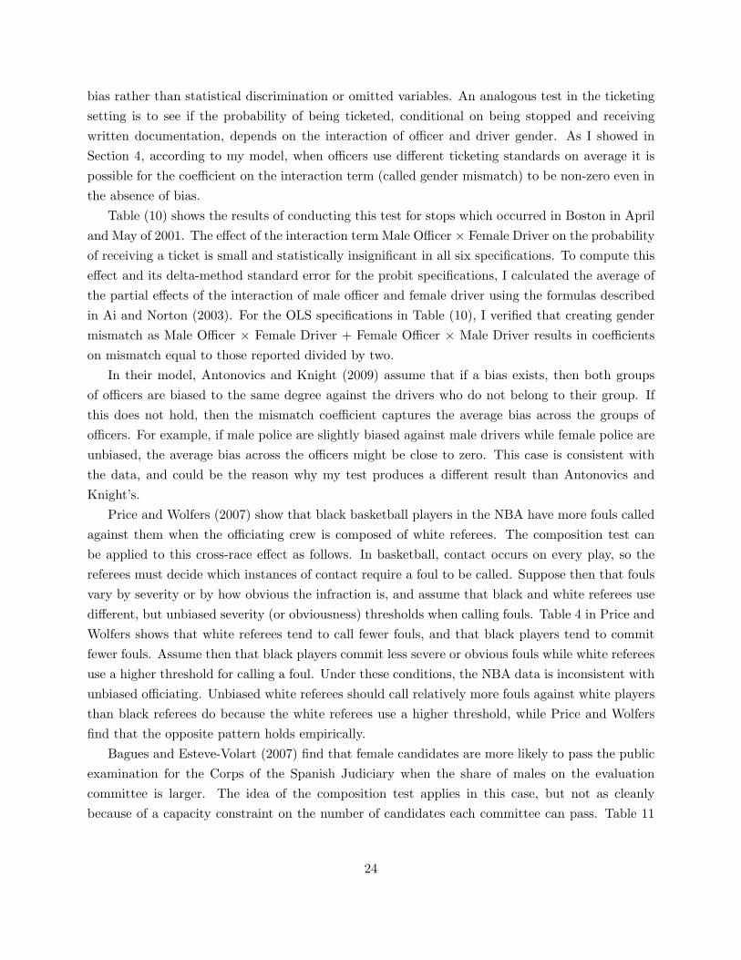
However, strategic driving with respect to gender seems less plausible. As Table (2) shows,

18Odds(pg) =P (T |df ,pg)

P (T |dm,pg)=

1−Ff{θ∗(df ,pg)}1−Fm{θ∗(dm,pg)} .

19This reasoning is similar to that of Grogger and Ridgeway (2006), who estimate how the odds that a stoppeddriver belongs a racial minority group depends on whether the stop occurred in daylight.

20This is becauseP (df |T )

P (dm|T )=

P (df |T )

1−P (df |T ).

14

female police officers are distributed fairly evenly across the Boston police districts, and are nevermore than 20% of the force in any district. In Boston, the chance of being observed by a femaleofficer is roughly uniform, which should make strategic driving simply not worthwhile.

In addition, since drivers cannot observe the gender of individual police officers before theydecide whether to break traffic laws, they cannot respond directly to officer gender. A directbehavioral response to gender or race is more likely in other settings, such as Price and Wolfers(2007) and Bagues and Esteve-Volart (2007), in which gender (or race) is randomly assigned butis visible to all participants before behavioral choices are made.21

Another potential problem is that female and male police officers may have different job func-tions, which might somehow cause female police to observe a different pool of drivers. Femaleofficers issued fewer traffic citations (see Table 1), which might indicate that job functions vary byofficer gender. Yet if female officers simply spend less time monitoring the roads than male officers,this does not invalidate the empirical strategy. For example, female officers were less likely to workat night, but conditioning on the time of the traffic ticket will account for how nighttime driversare different. In general, the inclusion of day of week and time of day controls, as well as day andtime interaction terms, will account for systematic differences in driver behavior during the timesthat male and female police are engaged in monitoring traffic.

Table (3) shows means of several work-related variables from the 2000 Census for male andfemale police in the Boston metropolitan area. Clearly, male officers spend significantly more timeon the job. Importantly, the higher hourly wage seen for male officers can be mostly explainedby the higher pay rate received for overtime, along with a smaller contribution due to the higherrate of college degree attainment for male officers. In the Boston Police Department, a collegedegree guarantees a 20% bonus over the base pay rate, while police receive 1.5 times their base payrate for overtime, which is hours worked in excess of 40 hours per week. Thus, the most prominentdifference in the Census data between male and female police officers is the number of hours workedper year, a difference which the empirical strategy is able to account for.

Figure (2) displays the time pattern of total citations by officer gender. Although fewer citationsare written by female police, the timing of the monthly fluctuations in citations matches up fairlywell. This indicates that male and female officers are subjected to the same shifts in policingactivity and driver behavior which account for the monthly changes in traffic tickets.

In their recruiting efforts, the Boston Police Department states that female officers are notpushed into systematically different or less desirable jobs than male officers.22 Furthermore, in

21In Price and Wolfers (2007), the NBA scheduling process guarantees that the racial makeup of the refereeingcrew is unrelated to the racial makeup of the teams. For Bagues and Esteve-Volart (2007), the Spanish governmentassigns candidates to committees without regard to the gender makeup of the committee.

22From the Boston P.D.’s Women in Policing web page: “Gone are the days of women serving solely in an ad-ministrative capacity or in positions deemed more suitable for women. Today we serve on the front lines. Womenon the job serve in various capacities such as patrol officers, criminal investigators, motorcycle officers, and hostagenegotiators.”

15

correspondence with the author, the Boston Police Department stated that: “Both male and femaleofficers perform the same functions within the Department.”

3.3 Results

Table (4) shows basic OLS and logit estimates for the effect of male officer on the probabilitythat the ticketed driver is female, with the sample split into speeding tickets and tickets for othertypes of violations. In the logit specification for speeding tickets with no controls, the odds ratiocoefficient on male police officer is not statistically different from 1. When miles-per-hour over thespeed limit is included, the ticketed driver is less likely to be female if the officer is male becausethe coefficient on male officer is less than 1 (0.808), an effect which is significant at the 1% level(s.e. = 0.057). The same pattern is observed in the OLS specifications for speeding tickets, whichalso provide a sense of the magnitude of the officer gender effect in terms of probabilities. If thepolice officer is male, the ticketed driver is about 5 percentage points less likely to be female, orequivalently 16 percent less likely to be female given that 30 percent of ticketed drivers are women.

The upward OLS bias towards zero results because miles-per-hour over the limit is negativelyrelated to both female driver and to male police officer. Thus, the observed OLS bias when miles-per-hour is omitted suggests two key observations. First, male police officers give tickets at lowervalues of miles-per-hour, indicating that they may use a lower threshold than female officers. Sec-ond, relatively fewer female drivers are found at higher miles-per-hour over the limit, which isconsistent with the MLRP assumption of the model.

For tickets issued for other traffic violations, such as failure to stop, no seat belt, or expiredinspection sticker, the results in Table (4) show that even when no control variables are used, malepolice officers ticketed relatively fewer female drivers, an effect which is significant at the 1% level.The magnitude of the effect is a bit smaller than that observed for speeding tickets; the ticketeddriver is 2.6 percentage points less likely to be female if the officer was male.

To link these results back to equation (7), note that because the odds ratio coefficient on maleofficer for speeding tickets is 0.808, this means EOdds(pm) = 0.808 ∗ EOdds(pf ). If male andfemale police officers observed the same pool of drivers, this would reflect how the odds of beingticketed conditional on being at risk depend on officer gender, so the result would imply thatOdds(pm) = 0.808 ∗Odds(pf ).

Linking the empirical odds directly to the ticketing odds requires assuming that male and femaleofficers observed the same pool of drivers, conditional on the set of observable characteristics ofeach traffic ticket. For this reason, I include a rich set of control variables: The speed limit of theroad, the driver’s race and age, driver’s age squared, whether the driver was from Boston (in-town),day of week dummies, weekend night and workday commute dummies, time of day dummies (pre-dawn, morning, afternoon, and evening), and dummies for the officer’s geographic district of theBoston Police Department. In addition, specifications including interactions of all day of week and

16

time of day dummies were estimated (these specifications do not include the workday commuteand weekend night dummies). If the estimated male officer effects in Table (4) were due to maleofficers observing a pool of drivers which systematically differed by these observable characteristics,including such controls would tend to push the male officer effects towards zero.

The results in Table (5) show that for both categories of tickets, the negative effect of maleofficer on the odds of the ticketed driver being female becomes only slightly smaller as controlsare included. In the specification for speeding tickets including the full set of controls, the oddsthat the driver is female falls by a factor of 0.845 (significant at the 5% level with s.e.=0.060) ifthe police officer is male. This estimate is within one standard error of the corresponding estimate(0.808) in Table (4) where the only control is miles-per-hour over the limit. The same pattern isseen in the results for other types of violations. This indicates that very little of the male officereffect is attributable to the effects of the control variables on the gender makeup of ticketed drivers.

To evaluate the robustness of these results, I estimated several alternative specifications. First,the log of the total number of traffic citations by month and Boston Police district was included asa control in both an OLS and a Logit specification. The number of tickets issued results from theinteraction of driver behavior with enforcement intensity, so periods with high numbers of ticketsissued must differ by at least one of these factors. Second, instead of the number of tickets by monthand district I used the number of tickets by officer and day. The coefficient on this ticket variablewill show how the gender mix of ticketed drivers depends on how many tickets the officer wrotethat day. Third, I included unrestricted dummies for each month in the data as controls, as Figure(2) showed significant variation in total citations in Boston over time. These dummies net out theimpact of monthly changes in the interaction of enforcement and driver behavior which drive theshifts in tickets, even though this is not necessarily desirable. For instance, if directed to write moretraffic tickets, gender-biased officers might respond by lowering their ticketing threshold for onlyone gender of drivers. The robustness specifications are estimated with day and time dummies,Boston district dummies, and controls for driver demographics.

The results of these robustness checks are shown in Table (6). Consistently across the differentspecifications, the number of tickets issued has an impact on the gender mix of ticketed drivers.Adding up tickets issued by either month and district or officer and day, when more tickets (eitherfor speeding or for other violations) were issued the ticketed driver was more likely to be female.The coefficients on male officer in these specifications are quite similar to those reported in Table(5). The only specification where the effect of male officer is attenuated is the specification forspeeding tickets with unrestricted month dummies, and even here the effect (odds ratio of 0.882)is only slightly smaller than in the baseline results and is still statistically significant at the 10%level.

To summarize, the empirical results confirm that male officers ticketed relatively fewer femaledrivers than female officers. The available evidence related to the activities of male and female

17

officers, together with the extensive controls to account for many factors which might plausiblyaffect the gender mix of drivers on the roads, suggest that this effect does not result becausemale and female police observed systematically different pools of drivers. I therefore conclude thatfemale drivers are less likely to be ticketed, conditional on committing a traffic violation, if theyare observed by a male police officer.

4 Application of the composition test

The next step in conducting the test is to rank the officer’s violation thresholds by determiningwhich officer gender must observe a more dangerous violation before deciding to issue a ticket. Byexamining the sample means in Table (1) and referring to Proposition (4), we could conclude thatmale officers use a lower ticketing threshold (they are “tough”) because they issued tickets for lowerfine amounts and lower miles-per-hour over the limit. This conclusion will be strengthened if it stillholds when extensive controls are used to account for possible differences in the pools of drivers atrisk.

For speeding tickets, I estimate OLS specifications for miles-per-hour over the limit as a functionof officer gender, the control variables used to estimate the officer-gender effect in Table (5), andtwo additional controls: The gender of the driver and an interaction of driver and officer gender.According to Proposition (4), driver gender can be omitted in order to rank officer’s thresholds,and specifications omitting driver gender (two are shown in Table (8), and others are available byrequest) produce the same rankings.23 I include driver gender and the interaction of driver andofficer gender (called “gender mismatch”) for comparison to Antonovics and Knight (2009). In theirmodel, the coefficient on mismatch of officer and driver race in a specification for the probability ofbeing searched captures taste-based discrimination. Therefore a statistically significant coefficienton gender mismatch might suggest that officers discriminate via the miles-per-hour they chargeticketed drivers with.

In my miles-per-hour specifications, because a dummy for male officers, a dummy for fe-male drivers, and their interaction (gender mismatch) are explanatory variables, the gender mis-match coefficient measures the following difference-in-difference: [mph(dm, pf ) − mph(df , pf )] −[mph(dm, pm)−mph(df , pm)]. Antonovics and Knight (2009) create their mismatch variable as thesum of two interaction terms: Black Officer × White Driver + White Officer × Black Driver. Ifcreated in this way, the gender mismatch coefficient would be equal to the difference-in-differenceshown above divided by two. The derivation of these equivalences are shown in the Appendix. Ineither case, the mismatch coefficient shows whether the average male driver versus female driverdisparity in miles-per-hour varies by officer gender. Analogously, Price and Wolfer’s (2007) interac-tion term of interest (the interaction of player race and referee crew race) captures how the racial

23Specifications using the percent over the limit as the dependent variable also produce the same rankings.

18

disparity in player foul rates varies by referee crew race. However, the ticketing model developedin Section 2 indicates that such variation by officer gender (or referee race) may not be due to biaswhen one group of officers (or referees) is tougher than the other.

To see this, consider a simple example in which the probability of receiving a ticket conditionalon breaking the law is known, so we can directly calculate P (T | dg, pg). Suppose these 4 quantitieswere observed: P (T | dm, pf ) = 0.3, P (T | df , pf ) = 0.1, P (T | dm, pm) = 0.5, and P (T | df , pm) =0.4. The male driver versus female driver disparity in this example is higher by 0.1 (which wouldbe the coefficient on gender mismatch) when the officer is female. Notice that male officers weretougher because they were always more likely to ticket violations. The tougher officers ticketedrelatively more female drivers, Odds(pm) = 0.4

0.5 > Odds(pf ) = 0.10.3 , so according to my test the

example is consistent with unbiased ticketing. Figure (3) illustrates this example graphically. Inthe Figure, the tough officer tickets drivers at 60 miles-per-hour while the easy officer tickets at70, and both officers are unbiased because they apply their thresholds equally to male and femaledrivers.

I rank officer’s violation thresholds for other types of traffic violations separately from speedingtickets, as there is no continuous measure which reflects the severity of violations such as “failure tostop” or “expired inspection sticker”. There is information on the dollar amount of the fine, whichis mostly determined by the specific offense the driver was charged with. Tickets for non-speedingviolations were by far most likely to impose a fine of either $25, $35, or $50.24 Because of thediscrete nature of the fine variable, I estimate ordered logit models for 5 fine amount categories:less than $26, from $26 to $35, from $36 to $50, from $51 to $100, and greater than $100. It isdifficult to interpret the effect of gender mismatch on the fine in the ordered logits, so I omit it fromthe reported ordered logit specifications. Instead, I report additional OLS specifications for the fineamount which include gender mismatch as an explanatory variable, and describe a calculation ofthe effect of gender mismatch based on an ordered logit in the text. Unfortunately the fine variableis missing for about 37% of the non-speeding tickets. The probability of the fine being missing isnegatively related to male officer, but the effect is small in magnitude (about 1.6 percentage points)so I ignore this issue here.

The results used for ranking officer’s ticketing thresholds are shown in Table (7). On average,conditional on all controls, male police issued speeding tickets for 1.47 fewer miles-per-hour overthe limit (standard error of 0.23) than the female officers. According to Proposition (4), we caninfer that male police use a lower ticketing threshold than the female police. The gender mismatchcoefficient, which captures the difference-in-difference described above, is small ( -0.47 miles-per-hour) and statistically insignificant. This might suggest that to the extent officers use discretion toassign miles-per-hour over the limit, they use this discretion similarly when faced with a driver ofthe opposite gender.

24Out of 68,759 non-speeding tickets with valid fine amount and gender data, 18.4% were for $25, 15.4% for $35,56.5% for $50, and 8.0% for $100.

19

The ordered logit and OLS results shown in Table (7) for other types of traffic citations againsuggest that male officers were tougher. The odds of the ticket being in a higher fine category(relative to all lower categories) falls by a factor of 0.66 (s.e.= 0.026) if the officer was male, whichis significant at the 5% level. Therefore, male officers were more likely to issue tickets for violationswhich imposed smaller fines, consistent with male officers using a lower ticketing threshold. TheOLS coefficient on gender mismatch when all controls are included is equal to 2.77 dollars with astandard error of 1.31. This could be reflecting a differential use of discretion to adjust chargedfines, but the effect is only about half the size of the main effect of male officer (-5.84 dollars). I alsoestimated the effect of gender mismatch on the fine by adding it as an explanatory variable to theordered logit model which includes controls in Table (7) and calculating the predicted fine amountfor each observation. I assumed the fines associated with the fine categories were the following:$25, $35, $50, $100, and $267.25 The average of the marginal effects of gender mismatch on thefine amount, accounting for the implied changes in the gender dummies, equals 1.08 dollars with abootstrapped (100 replications) standard error of 0.93.

The robustness of these results was tested by estimating a number of alternative specifications.First, I included the log of total citations issued by month and police district as an additionalcontrol. Second, I used the log of total citations by officer and day as a control, and also excludeddriver gender and gender mismatch as explanatory variables. Third, I put driver gender and gendermismatch back in and included unrestricted dummies for each month in the data. The results forthese specifications are shown in Table (8). The measures of tickets written had consistent effectsacross all the specifications. When more tickets were issued, ticketed violations occurred at lowermiles-per-hour and fine amounts. As we saw in the baseline specifications, for both speeding ticketsand other violations male officers tended to issue citations for relatively less serious offenses. Tothe extent possible with the available data it does not appear that this result occurs because maleofficers observed a different pool of drivers. The results therefore indicate that male officers aretougher because they are willing to write tickets for less dangerous violations.

Despite the consistent empirical pattern of male officers writing tickets for less serious violations,a relevant concern is that this may not reflect a difference in toughness but instead may result fromofficers adjusting miles-per-hour and fine amounts after deciding to write a ticket. Using the sameBoston data as this paper, Anbarci and Lee (2008) observe that for speeding tickets, the histogramof miles-per-hour over the limit spikes at 10. They argue that this represents officer discretionin giving some motorists a “discount” on their ticket, and they find that male officers are morelikely (by 33 percentage points) to write speeding tickets at exactly 10 miles-per-hour over the limit(when conditioning on the ticket being between 10 and 14 miles-per-hour over the limit).

Even accepting Anbarci and Lee’s interpretation that male officers are more likely to discountmiles-per-hour (this is not the main point of their paper), for several reasons I believe my results

25I used $267 for the highest category because it is the mean fine amount for non-speeding violations which receivedfines above $100.

20

imply that male officers are tougher. First, assuming that officers randomly chose violations between11 and 14 for discounting, Anbarci and Lee’s result implies that discounting would reduce chargedmiles-per-hour for male officers by 0.85 miles-per-hour.26 This cannot fully account for the maleofficer effect of -1.47 miles-per-hour in my baseline specifications. Second, there is no evidence ofdiscounting for offenses other than speeding. Fine amounts for these offenses are clustered at thevalues of very common infractions, such as “Failure to Stop” (about 25,000 observations) whichincurs a $50 fine in Massachusetts. Finally, discounting cannot explain why male officers wrotemore tickets (as shown in Table 1). In contrast, because tough officers are willing to ticket driversfor less serious offenses, for a given mix of offenses observed a tough officer will see more that exceedhis threshold and therefore issue more tickets. The three facts that male officers wrote tickets forlower miles-per-hour, lower fine amounts, and wrote more tickets (on days for which they issued atleast one) are all consistent with male officers being tough.

We can now conduct the composition test by combining the conclusion that male officers aretougher with the empirical results of Sections 3. The results in Section 3 indicate that male policeofficers were relatively less likely to ticket a female driver who committed a violation. Both of theseresults are statistically significant at the 5% level.27 According to the composition test, this patterncan only result if at least one gender group of officers is biased. The model implies that if therewas no bias, by using a lower ticketing threshold male officers should have been more likely thanfemale officers to ticket female drivers. Therefore, the null hypothesis that both officer genders areunbiased is rejected in favor of the alternative that at least one group of officers is gender biased.

Two critical assumption in the model are the MLRP and the average severity assumption.Besides suggesting the test for bias, the more general implication of these two assumptions is thatthere is a link between the gender composition of ticketed drivers and how fast (or expensive)ticketed violations are on average. If ticketed violations were slower on average, then relativelymore ticketed drivers should be female (and vice versa). The observed effects of the changes intotal tickets, added up by month and Boston police district or by officer and day, show a consistentpattern of empirical support for this link. When more tickets were issued, ticketed drivers weremore likely to be female, and ticketed violations occurred at lower miles-per-hour and fine categories(see Tables 6 and 8). These effects are statistically significant in all of the relevant specifications.

There are two potential explanations for how changes in the number of tickets issued couldproduce this pattern. First, the police might be lowering (or raising) their ticketing thresholds

26In the Boston data, male officers wrote speeding tickets to 1,609 drivers at 11 m.p.h. over, 2,272 at 12, 2,016 at13, and 2,162 at 14. From this, the average speed between 11 and 14 is 12.58. Male officers were more likely by afactor of 0.33 to mark the average 11 to 14 violation down to 10, so 0.33*(12.58-10)=0.8514 is the implied impact ofthe discounting.

27To assess the sensitivity of my standard errors, I estimated the baseline specifications in Tables 5 and 7 usingOLS and clustered the standard errors by officer. When clustering, the male officer coefficients in the specificationsfor miles-per-hour and fine amount are still significant at the 5% level. In the specifications for the probability thatthe ticketed driver is female, the male officer coefficients are significant at the 10% level (p-values between 0.067 and0.056).

21

in an unbiased fashion in order to write more (or fewer) tickets. Second, at certain times thereare sometimes more drivers at risk for a ticket and relatively more of them are female. Whicheverexplanation is correct, the pattern provides confidence in the validity of the link between the gendercomposition of ticketed drivers and the speed of ticketed violations which is implied by the model.

To get a sense of the quantitative impact of the bias, I construct a back-of-the-envelope cal-culation of the number of “excess tickets” resulting from gender bias. First, we must assumethere would be no behavioral response from drivers to the hypothetical policy change whichdrives the calculation.28 Next, if we assume that female police are unbiased and so use a sin-gle threshold θ∗(pf ), the pattern of violation thresholds consistent with the empirical results isθ∗(dm, pm) < θ∗(df , pm) < θ∗(pf ), meaning that male police are biased against male drivers. Usingthe point estimate of the male officer effect for non-speeding tickets in Table (5), we obtain thatEOdds(pm) = 0.9 ∗ EOdds(pf ). Note that EOdds(pm) =

Nmf

Nmm

, where Nmf is the number of female

drivers ticketed by male officers.Think of correcting the bias by lowering male officer’s threshold for females θ∗(df , pm) and

raising the threshold for males θ∗(dm, pm). The idea is that male police should have ticketed morefemale drivers and fewer male drivers. Holding the total number of tickets constant, let S representthe number of tickets to be shifted from males to females to equate the ticketing odds for maleofficers with that for female officers. We can do this by increasing the ticketing odds by a factor of1β , where β is the odds ratio coefficient on male officer. The calculation for S is therefore:

Nmf + S

Nmm − S

=1β

Nmf

Nmm

⇔ S =(1− β)Nm

m Nmf

βNmm + Nm

f

(9)

The ticketing model implies that S is a lower bound. If θ∗(dm, pm) was increased and θ∗(df , pm)was reduced until the two thresholds were equal, male officers using this new threshold θ∗(pm) wouldhave ticketed relatively more female drivers than the female police, because θ∗(pm) < θ∗(pf ). Fornon-speeding tickets with β = 0.9, S = 620. These 620 “shifted tickets” represent about 0.5% ofthe 110,556 non-speeding tickets issued during the 22 month sample period. The same calculationfor speeding tickets, with β = 0.85, results in S = 1, 282, which implies the shifted tickets are about3.5% of the the 36,343 speeding tickets issued during the sample period.

Alternatively, when assuming that male police are unbiased while female police are biased,the empirical results would imply that female police are biased against female drivers. Makinganalogous calculations, for non-speeding violations the number of tickets S to be shifted fromfemales to males is 100. For speeding tickets, S = 36. The quantitative impact of the gender biasis very small in this case because female officers issued relatively few traffic tickets.

28This would not be a good assumption if the policy change was large.

22

4.1 Relating the composition test to the existing literature

First I compare the composition test to a test for gender bias in ticketing which is analogous to thetest for racial bias in searches proposed in Anwar and Fang (2006). This test is based on Proposition(3), which suggests a test for gender bias based on comparing averages of miles-per-hour over thelimit (mph) for ticketed drivers in the following way pointed out by Anwar and Fang (2006):

Severity Test. At least one police officer gender is biased if:mph(dm, pm) > mph(dm, pf ) and mph(df , pm) < mph(df , pf ), or if:mph(dm, pm) < mph(dm, pf ) and mph(df , pm) > mph(df , pf ).

Critically, the severity test only compares average miles-per-hour for a gender group of ticketeddrivers across the officer genders. For the test to reject the null, there must be a switching ofthe rank orders for male versus female drivers. Comparing average miles-per-hour for male andfemale drivers within officer gender is not informative about the relative positions of the ticketingthresholds, because the distributions of violation severity are different for male and female drivers.

Table (9) shows the results of conducting the severity test for miles-per-hour and fine amount.As both the male and female drivers ticketed by the female police were ticketed at greater miles-per-hour than the drivers ticketed by males, the severity test does not reject the null hypothesis ofno gender bias in speeding tickets. The severity test also fails to reject the null for non-speedingviolations, because male officers wrote less expensive tickets to both driver genders. In addition,according to Proposition (3) this empirical pattern of sample means corroborates the conclusionthat male officers use a lower threshold on average (and therefore have a lower cost of ticketing onaverage). For this reason, the failure to reject the null hypothesis using Anwar and Fang’s test isnot surprising. Their test has zero power to detect bias when the groups of officers have differentcosts of ticketing on average, because there will never be a switching of rank orders even if onegroup of officers is biased.

Anwar and Fang conduct their test for bias by calculating rank orders of search rates andsuccess rates by officer race for each racial group of drivers.29 An analogous test for the ticketingoutcome is to rank P (T | dm, pm) versus P (T | dm, pf ), and P (T | df , pm) versus P (T | df , pf ). Ifthe ranking is different for male drivers than female drivers, then the null hypothesis of no genderbias is rejected. This test is not possible with the data at hand, but if the data were available forBoston we would expect this test to have zero power as well because male officers were tougher onaverage.

Antonovics and Knight (2009), using the same Boston Police Department data as I do, find thata search for contraband is more likely to be conducted when the race of the driver is different fromthe race of the police officer. Their theoretical model indicates that this cross-race effect is due to

29For example, in the absence of bias, if white officers are more likely than black officers to search black motorists,then white officers should also be more likely than black officers to search white motorists.

23

bias rather than statistical discrimination or omitted variables. An analogous test in the ticketingsetting is to see if the probability of being ticketed, conditional on being stopped and receivingwritten documentation, depends on the interaction of officer and driver gender. As I showed inSection 4, according to my model, when officers use different ticketing standards on average it ispossible for the coefficient on the interaction term (called gender mismatch) to be non-zero even inthe absence of bias.

Table (10) shows the results of conducting this test for stops which occurred in Boston in Apriland May of 2001. The effect of the interaction term Male Officer × Female Driver on the probabilityof receiving a ticket is small and statistically insignificant in all six specifications. To compute thiseffect and its delta-method standard error for the probit specifications, I calculated the average ofthe partial effects of the interaction of male officer and female driver using the formulas describedin Ai and Norton (2003). For the OLS specifications in Table (10), I verified that creating gendermismatch as Male Officer × Female Driver + Female Officer × Male Driver results in coefficientson mismatch equal to those reported divided by two.

In their model, Antonovics and Knight (2009) assume that if a bias exists, then both groupsof officers are biased to the same degree against the drivers who do not belong to their group. Ifthis does not hold, then the mismatch coefficient captures the average bias across the groups ofofficers. For example, if male police are slightly biased against male drivers while female police areunbiased, the average bias across the officers might be close to zero. This case is consistent withthe data, and could be the reason why my test produces a different result than Antonovics andKnight’s.

Price and Wolfers (2007) show that black basketball players in the NBA have more fouls calledagainst them when the officiating crew is composed of white referees. The composition test canbe applied to this cross-race effect as follows. In basketball, contact occurs on every play, so thereferees must decide which instances of contact require a foul to be called. Suppose then that foulsvary by severity or by how obvious the infraction is, and assume that black and white referees usedifferent, but unbiased severity (or obviousness) thresholds when calling fouls. Table 4 in Price andWolfers shows that white referees tend to call fewer fouls, and that black players tend to commitfewer fouls. Assume then that black players commit less severe or obvious fouls while white refereesuse a higher threshold for calling a foul. Under these conditions, the NBA data is inconsistent withunbiased officiating. Unbiased white referees should call relatively more fouls against white playersthan black referees do because the white referees use a higher threshold, while Price and Wolfersfind that the opposite pattern holds empirically.

Bagues and Esteve-Volart (2007) find that female candidates are more likely to pass the publicexamination for the Corps of the Spanish Judiciary when the share of males on the evaluationcommittee is larger. The idea of the composition test applies in this case, but not as cleanlybecause of a capacity constraint on the number of candidates each committee can pass. Table 11

24

in Bagues and Esteve-Volart shows that female candidates receive higher scores on average, andcommittees with more female members tend to assign higher scores. By using perhaps a lowerobjective standard, predominantly female committees might be expected to pass relatively moremales. However, then the predominantly female committees should pass more candidates total,which is not possible because committees are only permitted to pass a fixed number of candidates.

5 Conclusion

If the police are gender biased in their traffic ticketing decisions, then the disparate impact of trafficticketing on male drivers cannot be fully justified as resulting from the legitimate law enforcementobjective of promoting safety on the roads. This paper developed a model of police and driverbehavior which provides a testable implication of gender biased traffic ticketing. The test is basedon the model’s prediction that if the police are unbiased, the group of officers which is more reluctantto issue tickets should be relatively more likely to ticket male drivers who break the law. The testuses information on the miles-per-hour and fine amounts of ticketed violations to determine whichgroup of officers is more reluctant to issue tickets. I reject the null hypothesis of unbiased ticketingin Boston because female police were more reluctant to ticket but were also relatively more likelyto ticket female drivers. However, back of the envelope calculations based on the empirical resultssuggest the quantitative impact of the gender bias on traffic tickets received may be small. At leastin Boston, this suggests that the sizable gender disparity in traffic tickets may be mostly due todifferences in driving behavior by gender, rather than to biased policing.

Many empirical studies of discrimination estimate “cross-race” or “cross-gender” effects (thedifference-in-differences test). These cross effects show how an outcome for subjects (drivers, play-ers, candidates) depends on the racial or gender group of the evaluators (police, referees, committeemembers) who decide the outcome. The idea underlying this approach is that any dependence ofthe outcome on the pairing of subject and evaluator groups is difficult to explain as resulting fromstatistical discrimination or omitted variables. In my model, a cross-gender effect is generatedwhen male and female police use unbiased but different threshold rules to decide which drivers toticket. The test I developed in this paper offers a new method for determining if the directionof an observed cross effect is consistent with unbiased decision-making. The test can be appliedif the demographic groups of subjects are systematically different on the outcome of interest, ifa threshold decision rule is a reasonable approximation of the evaluator’s decision process, and ifthere is a plausible way to rank the evaluator’s thresholds.

25

6 Appendix

6.1 Proof of Proposition 2

∂Odds(pg)∂θ∗

=−ff (θ∗)[1− Fm{θ∗}] + fm(θ∗)[1− Ff{θ∗}]

(1− Fm{θ∗})2

=−ff (θ∗)

∫ ∞θ∗ fm(θ)dθ + fm(θ∗)

∫ ∞θ∗ ff (θ)dθ

(1− Fm{θ∗})2

=

∫ ∞θ∗ fm(θ∗)ff (θ)− ff (θ∗)fm(θ)dθ

(1− Fm{θ∗})2

< 0

The sign of the derivative is negative because by the MLRP ff (θ∗)fm(θ) > fm(θ∗)ff (θ), whichmakes the numerator negative.

6.2 Proof of Proposition 3

The average violation severity θ(dg, pg) for a threshold θ∗(dg, pg) is

θ = E[θ | θ∗, dg] =

∫ ∞θ∗ θfg(θ)dθ

1− Fg{θ∗}

The derivative of θ with respect to θ∗ is

∂θ

∂θ∗=

fg(θ∗)∫ ∞θ∗ fg(θ)[θ − θ∗]dθ

(1− Fg{θ∗})2> 0

The derivative is positive because θ > θ∗.

6.3 Proof of Proposition 4

The unbiased violation threshold is θ∗, and s(θ∗) = Nf

Nf+Nmis the share of ticketed drivers that are

female. The average violation severity for all drivers conditional on θ∗ is:

E[θ | θ∗] = s(θ∗)E[θ | θ∗, df ] + (1− s(θ∗))E[θ | θ∗, dm]

From Proposition (2) it can be shown that ∂s(θ∗)∂θ∗ < 0 (available by request). From Proposition (3)

we know that ∂E[θ|θ∗,dg ]∂θ∗ = ∂θ̄(dg)

∂θ∗ > 0. Compute the derivative:

∂E[θ | θ∗]∂θ∗

=∂s(θ∗)∂θ∗

[θ̄(df )− θ̄(dm)] + s(θ∗)∂θ̄(df )

∂θ∗+ [1− s(θ∗)]

∂θ̄(dm)∂θ∗

The last two terms are both positive, so ∂E[θ|θ∗]∂θ∗ is guaranteed to be positive if the first term is

greater than or equal to zero. This is satisfied if θ̄(dm) ≥ θ̄(df ).

26

6.4 Intepretation of gender mismatch coefficients

For the miles-per-hour (and fine amount) specifications, there are four key sample averages:

Male Officer Female OfficerMale Driver m1 m2

Female Driver m3 m4

I estimate OLS specifications of this form:

MPH = β0 + β1 ×Male Officer + β2 × Female Driver + β3 × (Male Officer× Female Driver) + ε

The equations for each sample average are therefore:

m1 = β0 + β1

m2 = β0

m3 = β0 + β1 + β2 + β3

m4 = β0 + β2

Substitute the other equations into the equation for m3:

β3 = m3 −m2 − [m1 −m2]− [m4 −m2]β3 = [m2 −m4]− [m1 −m3]β3 = [mph(dm, pf )−mph(df , pf )]− [mph(dm, pm)−mph(df , pm)]

When the gender mismatch variable is created analogously to the racial mismatch variable inAntonovics and Knight (2009), the OLS equation and the equations for each m are:

MPH = α0 + α1 ×Male Officer + α2 × Female Driver+ α3 × (Male Officer× Female Driver + Female Officer×Male Driver) + ε

m1 = α0 + α1

m2 = α0 + α3

m3 = α0 + α1 + α2 + α3

m4 = α0 + α2

Start with the equation for m3 and make substitutions:

α3 = m3 −m1 −m4 − α0

α3 = m3 −m1 −m4 + m2 − α3

α3 =[m2 −m4]− [m1 −m3]

2=

β3

2

27

7 Tables and Figures

Table 1: Sample means of traffic ticket variables by police officer gender.

Male Officers Female Officers

Female Driver 28.4% 30.5%Weekend 24.2% 21.2%Commute 55.4% 50.8%Daytime 66.8% 73.2%Speeding 25.0% 17.6%Failure to Stop 31.8% 32.1%No Inspection Sticker 8.9% 4.6%No Seat Belt 14.9% 5.8%MPH Over Limit (speeding) 14.3 15.4

(n=34,133) (n=923)

Fine Amount (non-speeding) $48.3 $55.8(n=68,090) (n=2,847)

Number of Citations 141,224 5,675Mean Citations per Officer-Day 9.5 4.9Tickets file merged with officer data, excludes cases where officer gender was missing.

Officer-Day: A calendar day in which the officer wrote at least one traffic ticket.

12.6% of the police officers are female.

28

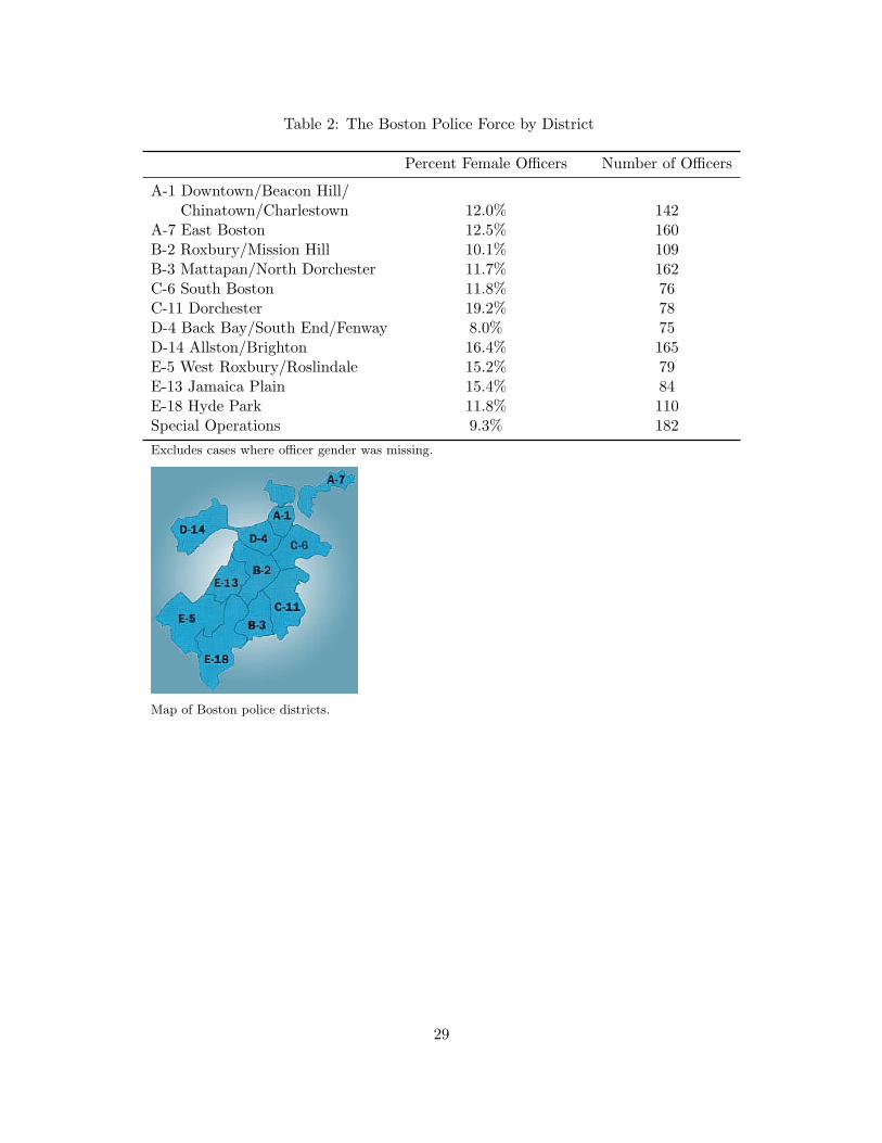
Table 2: The Boston Police Force by District

Percent Female Officers Number of Officers

A-1 Downtown/Beacon Hill/Chinatown/Charlestown 12.0% 142

A-7 East Boston 12.5% 160B-2 Roxbury/Mission Hill 10.1% 109B-3 Mattapan/North Dorchester 11.7% 162C-6 South Boston 11.8% 76C-11 Dorchester 19.2% 78D-4 Back Bay/South End/Fenway 8.0% 75D-14 Allston/Brighton 16.4% 165E-5 West Roxbury/Roslindale 15.2% 79E-13 Jamaica Plain 15.4% 84E-18 Hyde Park 11.8% 110Special Operations 9.3% 182Excludes cases where officer gender was missing.

Map of Boston police districts.

29

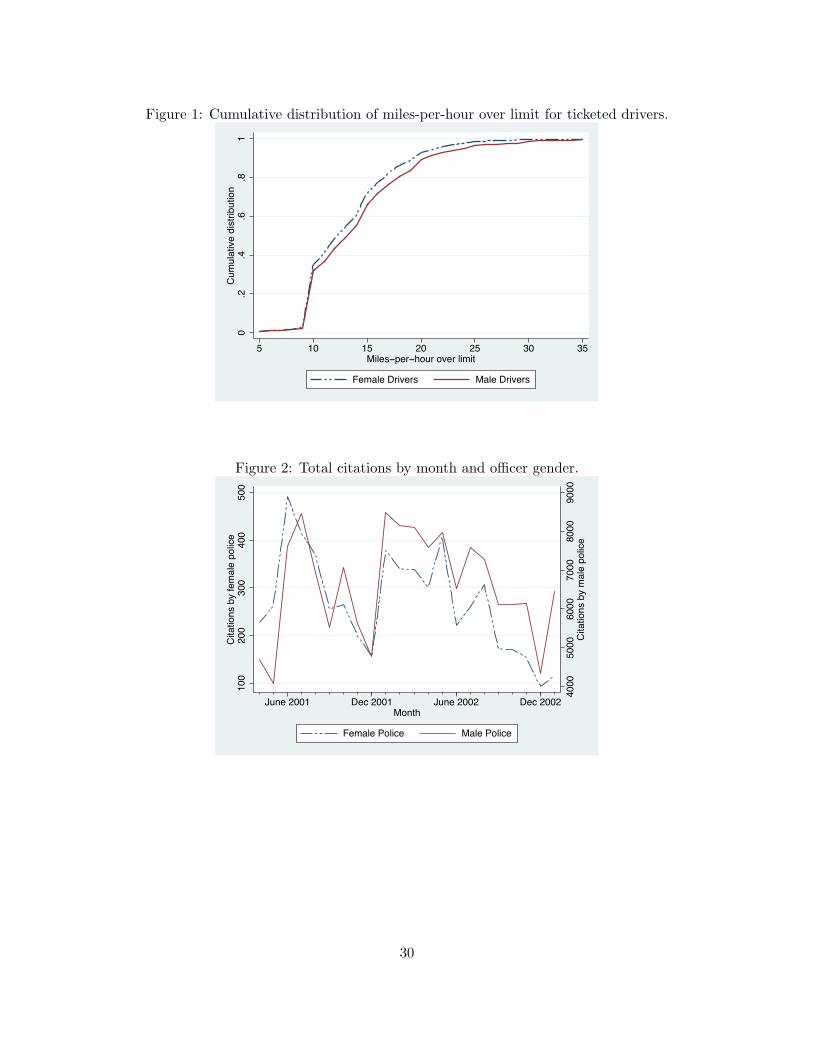
Figure 1: Cumulative distribution of miles-per-hour over limit for ticketed drivers.

0.2

.4.6

.81

Cum

ulat

ive

dist

ribut

ion

5 10 15 20 25 30 35Miles!per!hour over limit

Female Drivers Male Drivers

Figure 2: Total citations by month and officer gender.

4000

5000

6000

7000

8000

9000

Cita

tions

by

mal

e po

lice

100

200

300

400

500

Cita

tions

by

fem

ale

polic

e

June 2001 Dec 2001 June 2002 Dec 2002Month

Female Police Male Police

30

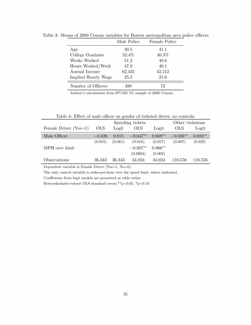
Table 3: Means of 2000 Census variables for Boston metropolitan area police officersMale Police Female Police

Age 40.5 41.1College Graduate 52.4% 40.3%Weeks Worked 51.2 48.6Hours Worked/Week 47.9 40.1Annual Income 62,435 42,152Implied Hourly Wage 25.5 21.6

Number of Officers 498 72Author’s calculations from IPUMS 5% sample of 2000 Census.

Table 4: Effect of male officer on gender of ticketed driver, no controls.Speeding tickets Other violations

Female Driver (Yes=1) OLS Logit OLS Logit OLS Logit

Male Officer −0.020 0.915 −0.047∗∗ 0.808∗∗ −0.026∗∗ 0.882∗∗

(0.015) (0.061) (0.016) (0.057) (0.007) (0.029)

MPH over limit −0.007∗∗ 0.966∗∗

(0.0004) (0.002)

Observations 36,343 36,343 34,024 34,024 110,556 110,556Dependent variable is Female Driver (Yes=1, No=0).

The only control variable is miles-per-hour over the speed limit, where indicated.

Coefficients from logit models are presented as odds ratios.

Heteroskedastic-robust OLS standard errors,**p<0.05, *p<0.10

31

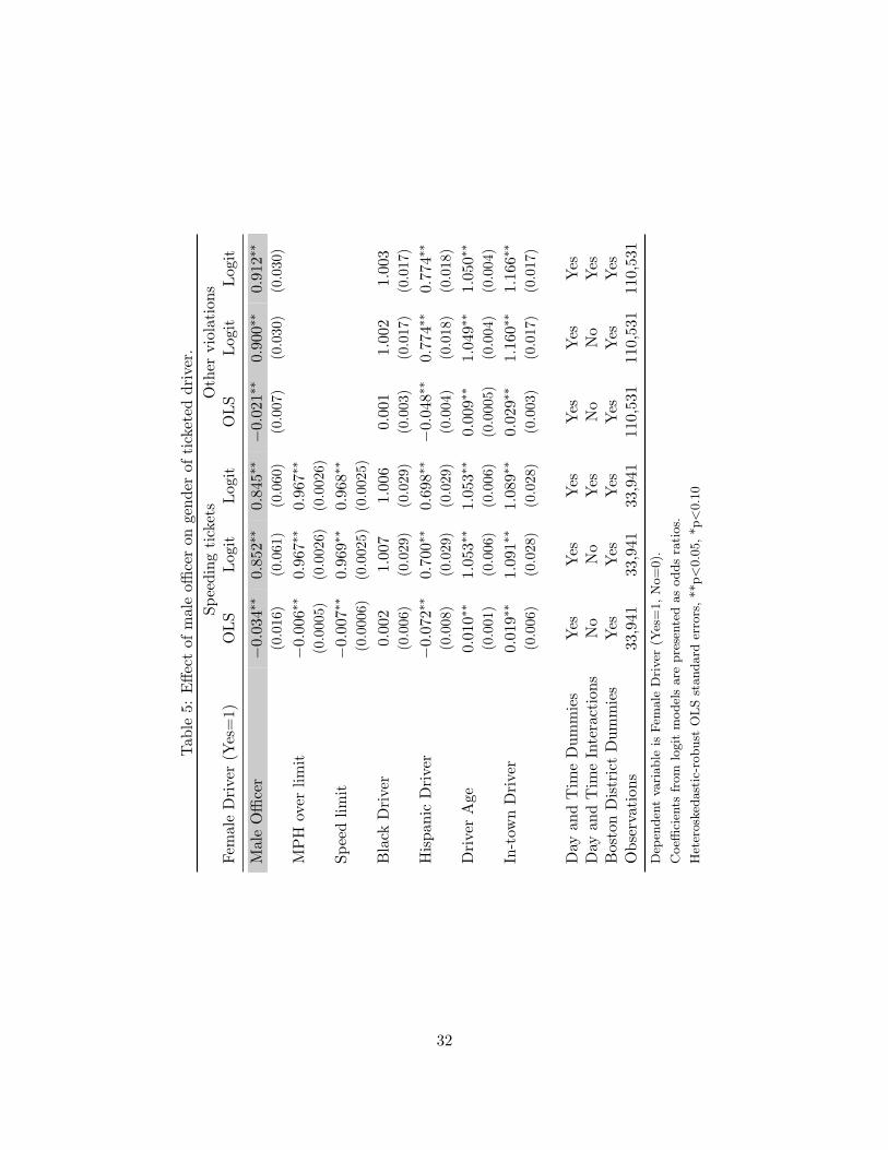
Tab

le5:

Effe

ctof

mal

eoffi

cer

onge

nder

ofti

cket

eddr

iver

.Sp

eedi

ngti

cket

sO

ther

viol

atio

nsFe

mal

eD

rive

r(Y

es=

1)O

LS

Log

itLog

itO

LS

Log

itLog

it

Mal

eO

ffice

r−

0.03

4∗∗

0.85

2∗∗

0.84

5∗∗

−0.

021∗

∗0.

900∗

∗0.

912∗

∗

(0.0

16)

(0.0

61)

(0.0

60)

(0.0

07)

(0.0

30)

(0.0

30)

MP

Hov

erlim

it−

0.00

6∗∗

0.96

7∗∗

0.96

7∗∗

(0.0

005)

(0.0

026)

(0.0

026)

Spee

dlim

it−

0.00

7∗∗

0.96

9∗∗

0.96

8∗∗

(0.0

006)

(0.0

025)

(0.0

025)

Bla

ckD

rive

r0.

002

1.00

71.

006

0.00

11.

002

1.00

3(0

.006

)(0

.029

)(0

.029

)(0

.003

)(0

.017

)(0

.017

)

His

pani

cD

rive

r−

0.07

2∗∗

0.70

0∗∗

0.69

8∗∗

−0.

048∗

∗0.

774∗

∗0.

774∗

∗

(0.0

08)

(0.0

29)

(0.0

29)

(0.0

04)

(0.0

18)

(0.0

18)

Dri

ver

Age

0.01

0∗∗

1.05

3∗∗

1.05

3∗∗

0.00

9∗∗

1.04

9∗∗

1.05

0∗∗

(0.0

01)

(0.0

06)

(0.0

06)

(0.0

005)

(0.0

04)

(0.0

04)

In-t

own

Dri

ver

0.01

9∗∗

1.09

1∗∗

1.08

9∗∗

0.02

9∗∗

1.16

0∗∗

1.16

6∗∗

(0.0

06)

(0.0

28)

(0.0

28)

(0.0

03)

(0.0

17)

(0.0

17)

Day

and

Tim

eD

umm

ies

Yes

Yes

Yes

Yes

Yes

Yes

Day

and

Tim

eIn

tera

ctio

nsN

oN

oY

esN

oN

oY

esB

osto

nD

istr

ict

Dum

mie

sY

esY

esY

esY

esY

esY

esO

bser

vati

ons

33,9

4133

,941

33,9

4111

0,53

111

0,53

111

0,53

1D

epen

den

tva

riable

isFem

ale

Dri

ver

(Yes

=1,N

o=

0).

Coeffi

cien

tsfr

om

logit

model

sare

pre

sente

das

odds

rati

os.

Het

erosk

edast

ic-r

obust

OLS

standard

erro

rs,**p<

0.0

5,*p<

0.1

0

32

Tab

le6:

Effe

ctof

mal

eoffi

cer

onge

nder

ofti

cket

eddr

iver

,ro

bust

ness

chec

ks.

Spee

ding

tick

ets

Oth

ervi

olat

ions

Fem

ale

Dri

ver

(Yes

=1)

OLS

Log

itLog

itLog

itO

LS

Log

itLog

itLog

it

Mal

eO

ffice

r−

0.03

2∗∗

0.86

0∗∗

0.82

8∗∗

0.88

2∗−

0.02

2∗∗

0.90

0∗∗

0.85

4∗∗

0.90

1∗∗

(0.0

16)

(0.0

61)

(0.0

60)

(0.0

64)

(0.0

07)

(0.0

30)

(0.0

29)

(0.0

30)

MP

Hov

erlim

it−

0.00

6∗∗

0.96

8∗∗

0.96

9∗∗

0.96

9∗∗

(0.0

005)

(0.0

03)

(0.0

03)

(0.0

03)

Log

(Tot

alC

itat

ions

)0.

026∗

∗1.

129∗

∗0.

015∗

∗1.

081∗

∗

bym

onth

and

dist

rict

(0.0

08)

(0.0

42)

(0.0

04)

(0.0

24)

Log

(Tot

alC

itat

ions

)1.

117∗

∗1.

106∗

∗

byoffi

cer

and

day

(0.0

18)

(0.0

09)

Sam

ple

Mon

thD

umm

ies

No

No

No

Yes

No

No

No

Yes

Day

and

Tim

eD

umm

ies

Yes

Yes

Yes

Yes

Yes

Yes

Yes

Yes

Bos

ton

Dis

tric

tD

umm

ies

Yes

Yes

Yes

Yes

Yes

Yes

Yes

Yes

Dri

ver

Dem

ogra

phic

sY

esY

esY

esY

esY

esY

esY

esY

esO

bser

vati

ons

33,9

4133

,941

33,9

4133

,491

110,

531

110,

531

110,

531

110,

531

Dep

enden

tva

riable

isFem

ale

Dri

ver

(Yes

=1,N

o=

0).

Coeffi

cien

tsfr

om

logit

model

sare

pre

sente

das

odds

rati

os.

Het

erosk

edast

ic-r

obust

OLS

standard

erro

rs,*

*p<

0.0

5,*p<

0.1

0

33

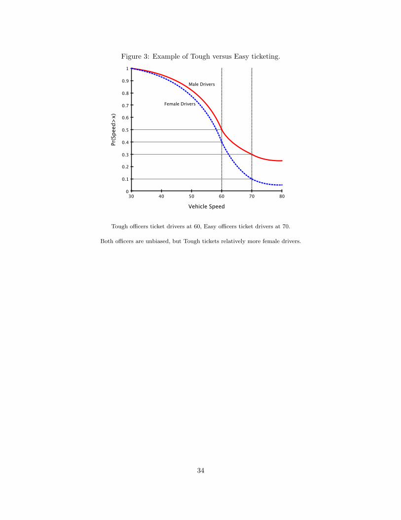
Figure 3: Example of Tough versus Easy ticketing.

8030 40 50 60 70

1

0

0.1

0.2

0.3

0.4

0.5

0.6

0.7

0.8

0.9

Vehicle Speed

Pr(S

peed

>x)

Male Drivers

Female Drivers

Tough officers ticket drivers at 60, Easy officers ticket drivers at 70.

Both officers are unbiased, but Tough tickets relatively more female drivers.

34

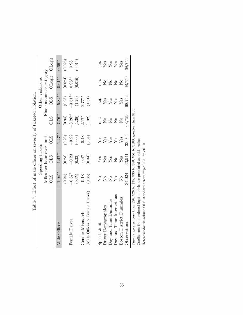
Tab

le7:

Effe

ctof

mal

eoffi

cer

onse

veri

tyof

tick

eted

viol

atio

n.Sp

eedi

ngti

cket

sO

ther

viol

atio

nsM

iles-

per-

hour

over

limit

Fin

eam

ount

orca

tego

ryO

LS

OLS

OLS

OLS

OLS

OLog

itO

Log

it

Mal

eO

ffice

r−

1.04

∗∗−

1.47

∗∗−

1.47

∗∗−

7.76

∗∗−

5.84

∗∗0.

61∗∗

0.66

∗∗

(0.2

4)(0

.23)

(0.2

3)(0

.94)

(0.9

3)(0

.024

)(0

.026

)

Fem

ale

Dri

ver

−0.

67∗

−0.

23−

0.22

−3.

26∗∗

−3.

51∗∗

0.96

∗∗0.

98(0

.35)

(0.3

3)(0

.33)

(1.3

0)(1

.29)

(0.0

16)

(0.0

16)

Gen

der

Mis

mat

ch-0

.18

-0.4

7-0

.48

2.17

∗2.

77∗∗

(Mal

eO

ffice

r×

Fem

ale

Dri

ver)

(0.3

6)(0

.34)

(0.3

4)(1

.32)

(1.3

1)

Spee

dLim

itN

oY

esY

esn.

a.n.

a.n.

a.n.

a.D

rive

rD

emog

raph

ics

No

Yes

Yes

No

Yes

No

Yes

Day

and

Tim

eD

umm

ies

No

Yes

Yes

No

Yes

No

Yes

Day

and

Tim

eIn

tera

ctio

nsN

oN

oY

esN

oY

esN

oY

esB

osto

nD

istr

ict

Dum

mie

sN

oY

esY

esN

oY

esN

oY

esO

bser

vati

ons

34,0

2433

,941

33,9

4168

,759

68,7

4468

,759

68,7

44Fin

eca

tegori

es:

less

than

$26,$26

to$35,$36

to$50,$51

to$100,gre

ate

rth

an

$100.

Coeffi

cien

tsfr

om

ord

ered

logit

model

sare

pre

sente

das

odds

rati

os.

Het

erosk

edast

ic-r

obust

OLS

standard

erro

rs,*

*p<

0.0

5,*p<

0.1

0

35

Tab

le8:

Effe

ctof

mal

eoffi

cer

onse

veri

tyof

tick

eted

viol

atio

n,ro

bust

ness

chec

ks.

Spee

ding

tick

ets

Oth

ervi

olat

ions

Mile

s-pe

r-ho

urov

erlim

itFin

eam

ount

orca

tego

ryO

LS

OLS

OLS

OLS

OLS

OLS

OLog

itO

Log

it

Mal

eO

ffice

r−

1.51

∗∗−

1.57

∗∗−

1.69

∗∗−

5.82

∗∗−

3.91

∗∗−

5.77

∗∗0.

67∗∗

0.67

∗∗

(0.2

3)(0

.18)

(0.2

3)(0

.93)

(0.7

0)(0

.94)

(0.0

26)

(0.0

27)

Fem

ale

Dri

ver

−0.

22−

0.23

−3.

42∗∗

−3.

43∗∗

0.99

0.99

(0.3

3)(0

.33)

(1.2

9)(1

.29)

(0.0

17)

(0.0

17)

Gen

der

Mis

mat

ch-0

.48

-0.4

42.

68∗∗

2.70

∗∗

(Mal

eO

ffice

r×

Fem

ale

Dri

ver)

(0.3

4)(0

.33)

(1.3

1)(1

.32)

Log

(Tot

alC

itat

ions

)−

0.61

∗∗−

0.64

∗0.

88∗∗

bym

onth

and

dist

rict

(0.0

83)

(0.3

3)(0

.020

)

Log

(Tot

alC

itat

ions

)−

0.36

∗∗−

2.83

∗∗

byoffi

cer

and

day

(0.0

4)(0

.13)

Spee

dLim

itY

esY

esY

esn.

a.n.

a.n.

a.n.

a.n.

a.Sa

mpl

eM

onth

Dum

mie

sN

oN

oY

esN

oN

oY

esN

oY

esD

rive

rD

emog

raph

ics

Yes

Yes

Yes

Yes

Yes

Yes

Yes

Yes

Day

and

Tim

eD

umm

ies

Yes

Yes

Yes

Yes

Yes

Yes

Yes

Yes

Bos

ton

Dis

tric

tD

umm

ies

Yes

Yes

Yes

Yes

Yes

Yes

Yes

Obs

erva

tion

s33

,941

34,9

7033

,941

68,7

4470

,921

68,7

4468

,744

68,7

44Fin

eca

tegori

es:

less

than

$26,$26

to$35,$36

to$50,$51

to$100,gre

ate

rth

an

$100.

Coeffi

cien

tsfr

om

ord

ered

logit

model

sare

pre

sente

das

odds

rati

os.

Het

erosk

edast

ic-r

obust

OLS

standard

erro

rs,*

*p<

0.0

5,*p<

0.1

0

36

Table 9: Tests analogous to Anwar and Fang (2006).Male Officers Female Officers p-value

Miles-per-hourMale Drivers 14.5 15.6 < 0.001

Female Drivers 13.7 14.9 < 0.001

Fine amountMale Drivers 48.6 56.3 < 0.001

Female Drivers 47.5 53.1 < 0.001p-values for null that mean differences are not different from zero.

Average miles-per-hour for speeding violations, fine amount for other violations.

37

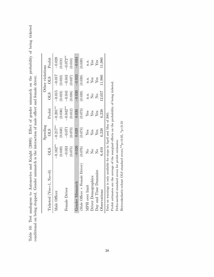
Tab

le10

:Tes

tan

alog

ous

toA

nton

ovic

san

dK

nigh

t(2

009)

:E

ffect

ofge

nder

mis

mat

chon

the

prob

abili

tyof

bein

gti

cket

edco

ndit

iona

lon

bein

gst

oppe

d.G

ende

rm

ism

atch

isth

ein

tera

ctio

nof

mal

eoffi

cer

and

fem

ale

driv

er.

Spee

ding

Oth

ervi

olat

ions

Tic

kete

d(Y

es=

1,N

o=0)

OLS

OLS

Pro

bit

OLS

OLS

Pro

bit

Mal

eO

ffice

r−

0.16

2∗∗

−0.

217∗

∗−

0.20

1∗∗

−0.

015

−0.

017

−0.

028

(0.0

49)

(0.0

48)

(0.0

36)

(0.0

23)

(0.0

23)

(0.0

18)

Fem

ale

Dri

ver

−0.

031

−0.

071

−0.

042∗

∗−

0.04

1−

0.04

1−

0.07

2∗∗

(0.0

75)

(0.0

73)

(0.0

12)

(0.0

38)

(0.0

37)

(0.0

10)

Gen

der

Mis

mat

ch−

0.02

60.

029

0.03

0−

0.03

0−

0.03

3−

0.03

4(M

ale

Offi

cer×

Fem

ale

Dri

ver)

(0.0

76)

(0.0

74)

(0.0

73)

(0.0

39)

(0.0

39)

(0.0

39)

MP

Hov

erlim

itN

oY

esY

esn.

a.n.

a.n.

a.D

rive

rD

emog

raph

ics

No

Yes

Yes

No

Yes

Yes

Day

and

Tim

eD

umm

ies

No

Yes

Yes

No

Yes

Yes

Obs

erva

tion

s6,

410

6,23

86,

238

12,0

5711

,980

11,9

80D

ata

on

warn

ings

isonly

available

for

stops

inA

pri

land

May

of2001.

Pro

bit

esti

mate

sare

the

aver

age

ofth

em

arg

inaleff

ects

on

the

pro

bability

ofbei

ng

tick

eted

.

Del

ta-m

ethod

standard

erro

rsfo

rpro

bit

esti

mate

s.

Het

erosk

edast

ic-r

obust

OLS

standard

erro

rs,*

*p<

0.0

5,*p<

0.1

0

38

8 References

Ai, Chunrong and Norton, Edward. “Interaction Terms in Logit and Probit Models”, EconomicsLetters 2003.

Anbarci, Nejat and Lee, Jungmin. “Speed Discounting and Racial Disparities: Evidence fromSpeeding Tickets in Boston”, IZA Discussion paper 3903, December 2008.

Antonovics, Kate and Knight, Brian. “A New Look at Racial Profiling: Evidence from the BostonPolice Department”, Review of Economics and Statistics, February 2009.

Anwar, Shamena and Fang, Hanming. “An Alternative Test of Racial Prejudice in Motor VehicleSearches: Theory and Evidence”, American Economic Review, March 2006.

Ayres, Ian. “Outcome Tests of Racial Disparities in Police Practices”, Justice Research and Policy,Fall 2002.

Bagues, Manuel and Esteve-Volart, Berta. “Can Gender Parity Break the Glass Ceiling? Evidencefrom a repeated randomized experiment”, Working paper, June 2007.

Becker, Gary. “The Economics of Discrimination”, University of Chicago Press, 1957.Blackmon, B. Glenn and Zeckhauser, Richard. “Mispriced Equity: Regulated Rates for Auto

Insurance in Massachusetts”, American Economic Review, Papers and Proceedings, May 1991.Blalock, Garrik; Jed DeVaro; Stephanie Leventhal; Daniel Simon. “Gender Bias in Power Rela-

tionships: Evidence from Police Traffic Stops”, Working paper, Feb. 2007.Dedman, Bill and Latour, Francie. “Race, sex, and age drive ticketing”, The Boston Globe, July

20 2003.Dedman, Bill. “Boston police to get tough on tickets”, The Boston Globe, Jan. 17 2004.Dharmapala, Dhammika and Ross, Steven. “Racial Bias in Motor Vehicle Searches: Additional

Theory and Evidence”, Contributions to Economic Analysis and Policy, 2004.Durose, Matthew; Erica Smith; Patrick Langan. “Contacts between Police and the Public, 2005”.

U.S. Department of Justice, Bureau of Justice Statistics, Special Report. April 2007.Farrell, Amy; Dean McDevitt; Lisa Bailey; Carsten Andresen; Erica Pierce. “Massachusetts Racial

and Gender Profiling Final Report: Executive Summary”, Northeastern University Instituteon Race and Justice, May 2004.

Grogger, Jeffrey and Ridgeway, Greg. “Testing for Racial Profiling in Traffic Stops from Behind aVeil of Darkness”, Journal of the American Statistical Association, Sept. 2006.

Edlin, Aaron and Karaca-Mandic, Pinar. “The Accident Externality from Driving”, Journal ofPolitical Economy, 2006.

Knowles, John; Nicola Persico; Petra Todd. “Racial Bias in Motor Vehicle Searches: Theory andEvidence”, Journal of Political Economy, Feb. 2001.

Levitt, Steven and Porter, Jack. “How Dangerous are Drinking Drivers?”, Journal of PoliticalEconomy, 2001.

39

Makowsky, Michael and Stratmann, Thomas. “Political Economy at Any Speed: What DeterminesTraffic Citations?”, American Economic Review, March 2009.

National Highway Traffic Safety Administration, Center for Statistics and Analysis. “2006 AnnualAssessment of Motor Vehicle Crashes.” Sept. 2007.

Price, Joseph and Wolfers, Justin. “Racial Discrimination Among NBA Referees”, NBER workingpaper 13206, June 2007.

Rowe, Brian. ”Discretion and Ulterior Motives in Traffic Stops: The Detection of Other Crimesand the Revenue from Tickets”, Working paper, April 2009.

Schanzenbach, Max. “Racial and Sex Disparities in Prison Sentences: The Effect of District-LevelJudicial Demographics”, Journal of Legal Studies, Jan. 2005.

40