1

Dynamic Loads Analysis Using Detailed Aircraft and

Landing Gear Modeling

Phillip W. Richards1 and Andrew Erickson

2

SDI Engineering Inc., Kirkland, WA, 98033, USA

Modern aircraft landing gears consist of many complex, nonlinear subsystems including

the landing gear structure, shock absorber, hydraulic steering, braking, antiskid system and

tires. SDI Engineering has developed a landing gear modeling and simulation software tool

called GearSim that includes detailed models of the relevant landing gear subsystems,

including the shock absorber, tire and leg flexibility, as well as aeroservoelastic modeling

capability for the airframe and the flight control system. A realistic model of a commercial

transport airplane was built with GearSim to study the effects of aircraft and landing gear

subsystem dynamics on landing loads.

I. Nomenclature

Ci,j = aerodynamic derivative of force/moment i with respect to j

c = damping coefficient in oleo model, kg/m

D = drag force on airplane, N

d = oleo stroke length, m

F = force produced by oleo, N

g = acceleration due to gravity, m/s2

Iy = aircraft pitch inertia, kg m2

K = flight control gain, appropriate dimension

L = lift force on airplane, N

M = three moment components on airplane, Nm

p = aircraft roll rate, rad/s

q = aircraft pitch rate, rad/s

r = aircraft yaw rate, rad/s, or tire radius, m

S = wing planform area, m2

s = oleo closure position, m

V = velocity of either aircraft or tire, m/s

Y = side force on airplane, N

𝛼 = aircraft angle of attack, rad

𝛼𝑠 = tire slip angle, rad

𝛽 = aircraft sideslip angle, rad

𝛿 = deflection of aileron, elevator, rudder, or spoiler, rad

𝜃 = pitch angle of aircraft, rad

𝜌 = air density, kg/m3

𝜎 = tire slip ratio, dimensionless

Ω = tire rotational speed, rad/s

II. Introduction

The aircraft certification process requires a significant number of flight and ground tests to ensure the aircraft’s

structure and landing gear perform safely under a wide range of operations. A reduction of the required number of

test points in flight and ground tests will save significant cost and time during the design and analysis process, and

can be achieved by using a reliable and accurate simulation capability. In addition, ground test simulations can

1 Principal Aeronautical Engineer, prichards@sdi-eng.com, AIAA Member

2 Principal Aeronautical Engineer, aerickson@sdi-eng.com, AIAA Member

2

provide improved prediction and understanding of extreme or difficult to obtain cases such as strong crosswinds,

variable runway conditions, hard landings, and abrupt maneuvers.

The industry standard methods for the prediction of loads during ground operations are typically based on static

force balances of the aircraft (Ref. [1]). However, dynamic effects could be included in ground loads analyses as

they can lead to loads exceedances and possible fatigue issues. The ground loads analysis process can be improved

with accurate modeling of landing gear dynamics, aeroservoelastic effects, runway conditions, wind strength and

direction, and the forced displacement that drives the landing gear. The loads during landing depend on the

aerodynamic conditions and approach maneuver implemented by the pilot. The touchdown velocity of the aircraft is

a critical parameter in the magnitude and character of the dynamic landing loads. Crosswind conditions, turbulence,

or discrete gust encounters can also influence the ground loads. Crosswind conditions can be particularly

challenging to model because the approach maneuver can vary based on pilot preference or operational

requirements.

Interactions between the many complex, nonlinear subsystems that comprise the landing gear and the aircraft can

lead to undesirable phenomena such as shimmy, braking-induced vibration, and accelerated tire wear or blowout.

Including all of these effects will significantly improve the accuracy of individual subsystem models and the

comprehensive ground loads analysis. This integrated capability allows for the evaluation of individual subsystem

performance as well as the complex interactions that can lead to performance degradation of the entire landing gear.

The development of a commercial ground loads analysis software tool is necessary because the methods and tools

used by aircraft, landing gear and landing gear subsystem manufacturers are typically proprietary; engineering teams

are therefore required to use their own aircraft loads analysis tools.

SDI Engineering has developed GearSim, which is an integrated software tool for landing gear subsystem and

ground loads analysis. GearSim is based in MATLAB/Simulink and consists of Simulink library blocks to model the

relevant landing gear subsystems. GearSim can be used in applications ranging from a detailed system level landing

gear analysis to the evaluation of aircraft ground loads. The software has been developed over many years and

recently in collaboration with the US Air Force (USAF) and Airbus Americas Inc. These partnerships have provided

a unique opportunity to validate the software for military and commercial aircraft. The original development efforts

were supported by Phase I and Phase II Small Business Innovation Research (SBIR) programs through the US Air

Force Test Center (AFTC) at Edwards Air Force Base (AFB). GearSim has recently been further developed through

an ongoing sponsorship from the Landing Gear Test Facility (LGTF) at Wright-Patterson AFB that has also

provided the opportunity to validate GearSim’s landing gear analysis against test data. Specifically, LGTF has aided

in validation of the vertical tire model, the shock absorber performance, and an individual landing gear drop test.

Airbus Americas Inc. has also been involved during the latest SBIR phase, providing feedback on GearSim’s

capabilities and further validation of the software.

This study focuses on dynamic landing loads for a mid-size transport aircraft. First, a representative aircraft and

landing gear model is presented. Then, two cases of dynamic loads analysis are presented: Landing with a brake

application, and landing in crosswind conditions.

III. GearSim: Landing Gear and Ground Loads Predictive Analysis

GearSim combines a high fidelity, nonlinear, six degree-of-freedom (6-DOF) landing gear system modeling tool

with variable fidelity aeroelastic and flight control system simulation tools, in order to produce an efficient and

accurate integrated simulation. Specifically, the simulation tool is compatible with a Nastran generated linear

aeroelastic model for simpler problems, and has the ability to couple with full nonlinear aeroelastic simulation tools

for highly complex, nonlinear, time-varying problems.

Because GearSim is based in MATLAB/Simulink, users are provided easy access to a wide variety of industry

standard engineering tools. Simulink contains many robust solvers to integrate the equations of motion, and the

Simulink model provides a visual understanding of the interplay of subsystems. Users can easily connect their own

proprietary analysis tools with the GearSim subsystem library blocks, allowing full control over the definition of

specific subsystems.

The dynamic equations of the landing gear subsystems are modularized in Simulink library blocks. Subsystems

such as the leg structure and bracing, shock absorber, and steering and braking systems are defined by engineering

parameters readily available from the relevant drawings and specifications. The Graphical User Interface (GUI)

consists of a series of menus that guide the user through the landing gear configuration and definition of all relevant

subsystems, and then a Simulink model is automatically generated using the library of subsystem blocks. A

screenshot of the GUI interface is provided in Fig. 1. The top-level Simulink model contains an aircraft block and a

landing gear block for each leg. Each landing gear block contains further blocks representing each of the subsystems

3

associated with that landing gear. The simulation can be run and post-processed within the GUI, providing relevant

loads and stability results at the click of a button.

Fig. 1 GearSim user interface

Both a rigid and an aeroelastic model are available for the aircraft representation. The rigid aircraft model

includes 6-DOF dynamics, with the option to conduct symmetric (3-DOF) analyses. The aircraft model includes a

pitch control system to maintain trim and perform the aircraft derotation maneuver after landing, and a

lateral/directional control system to maintain lateral trim and perform any lateral maneuvers, such as in a crosswind

landing. The initial conditions of the aircraft are determined by a trimming feature built into GearSim so that the

aircraft begins at a steady, level flight condition at a prescribed total velocity and sink rate. The pitch attitude, angle

of attack, thrust, and elevator settings are determined by the trimming routine in the symmetric case, and in the full

6-DOF case, the trim routine also determines the sideslip angle, rudder/aileron deflection, and asymmetric thrust

setting.

GearSim also includes the option to replace the rigid aircraft model with an externally provided aeroelastic

model. This capability is designed to interface with Nastran, but any aeroelastic software program may be used to

provide the aeroelastic matrices. These matrices are imported into GearSim and the aircraft flexible equations of

motion are integrated simultaneously with the landing gear dynamics.

IV. Aircraft and Landing Gear Model Development

One of the challenges in detailed modeling of landing gear systems is the availability of relevant information for

the subsystem models. GearSim includes a library of landing gear types and simple design routines that can guide

the user towards choosing the appropriate modeling parameters for each landing gear. This section defines a

representative narrow-body commercial aircraft and landing gear model suitable for dynamic landing loads analysis.

The representative aircraft defined in this section is based information obtained from the public domain. This model

is not intended as an exact model of any particular aircraft, but only a representative model that has been used to

analyze the general behavior of this class of aircraft.

A. Aircraft Characteristics and Landing Gear Layout

Weight and geometric information for the representative aircraft were obtained using Ref. [2]. A generic 3-view

of a representative commercial narrow-body aircraft was used to estimate the mean aerodynamic chord location of

the wing; the center of gravity (CG) of the aircraft was assumed to be at the quarter-chord of the mean aerodynamic

4

chord. This technique was also used to estimate the position of the landing gears with respect to the CG. The

maximum landing weight, CG location, and relative locations of the main and nose landing gears were used in a

static force balance to determine the static load on the main and nose landing gears.

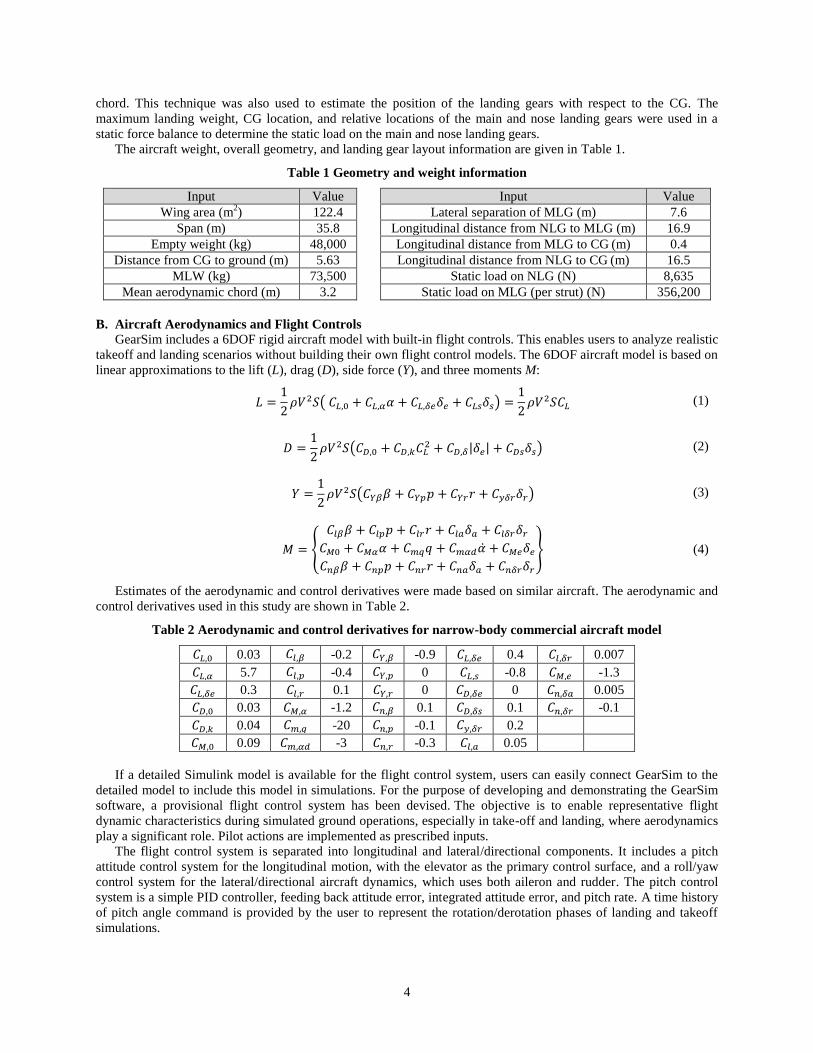
The aircraft weight, overall geometry, and landing gear layout information are given in Table 1.

Table 1 Geometry and weight information

Input Value Input Value

Wing area (m2) 122.4 Lateral separation of MLG (m) 7.6

Span (m) 35.8 Longitudinal distance from NLG to MLG (m) 16.9

Empty weight (kg) 48,000 Longitudinal distance from MLG to CG (m) 0.4

Distance from CG to ground (m) 5.63 Longitudinal distance from NLG to CG (m) 16.5

MLW (kg) 73,500 Static load on NLG (N) 8,635

Mean aerodynamic chord (m) 3.2 Static load on MLG (per strut) (N) 356,200

B. Aircraft Aerodynamics and Flight Controls

GearSim includes a 6DOF rigid aircraft model with built-in flight controls. This enables users to analyze realistic

takeoff and landing scenarios without building their own flight control models. The 6DOF aircraft model is based on

linear approximations to the lift (L), drag (D), side force (Y), and three moments M:

𝐿 =1

2𝜌𝑉2𝑆( 𝐶𝐿,0 + 𝐶𝐿,𝛼𝛼 + 𝐶𝐿,𝛿𝑒𝛿𝑒 + 𝐶𝐿𝑠𝛿𝑠) =

1

2𝜌𝑉2𝑆𝐶𝐿 (1)

𝐷 =1

2𝜌𝑉2𝑆(𝐶𝐷,0 + 𝐶𝐷,𝑘𝐶𝐿

2 + 𝐶𝐷,𝛿|𝛿𝑒| + 𝐶𝐷𝑠𝛿𝑠) (2)

𝑌 =1

2𝜌𝑉2𝑆(𝐶𝑌𝛽𝛽 + 𝐶𝑌𝑝𝑝 + 𝐶𝑌𝑟𝑟 + 𝐶𝑦𝛿𝑟𝛿𝑟) (3)

𝑀 = {

𝐶𝑙𝛽𝛽 + 𝐶𝑙𝑝𝑝 + 𝐶𝑙𝑟𝑟 + 𝐶𝑙𝑎𝛿𝑎 + 𝐶𝑙𝛿𝑟𝛿𝑟

𝐶𝑀0 + 𝐶𝑀𝛼𝛼 + 𝐶𝑚𝑞𝑞 + 𝐶𝑚𝛼𝑑�̇� + 𝐶𝑀𝑒𝛿𝑒

𝐶𝑛𝛽𝛽 + 𝐶𝑛𝑝𝑝 + 𝐶𝑛𝑟𝑟 + 𝐶𝑛𝑎𝛿𝑎 + 𝐶𝑛𝛿𝑟𝛿𝑟

} (4)

Estimates of the aerodynamic and control derivatives were made based on similar aircraft. The aerodynamic and

control derivatives used in this study are shown in Table 2.

Table 2 Aerodynamic and control derivatives for narrow-body commercial aircraft model

𝐶𝐿,0 0.03 𝐶𝑙,𝛽 -0.2 𝐶𝑌,𝛽 -0.9 𝐶𝐿,𝛿𝑒 0.4 𝐶𝑙,𝛿𝑟 0.007

𝐶𝐿,𝛼 5.7 𝐶𝑙,𝑝 -0.4 𝐶𝑌,𝑝 0 𝐶𝐿,𝑠 -0.8 𝐶𝑀,𝑒 -1.3

𝐶𝐿,𝛿𝑒 0.3 𝐶𝑙,𝑟 0.1 𝐶𝑌,𝑟 0 𝐶𝐷,𝛿𝑒 0 𝐶𝑛,𝛿𝑎 0.005

𝐶𝐷,0 0.03 𝐶𝑀,𝛼 -1.2 𝐶𝑛,𝛽 0.1 𝐶𝐷,𝛿𝑠 0.1 𝐶𝑛,𝛿𝑟 -0.1

𝐶𝐷,𝑘 0.04 𝐶𝑚,𝑞 -20 𝐶𝑛,𝑝 -0.1 𝐶𝑦,𝛿𝑟 0.2

𝐶𝑀,0 0.09 𝐶𝑚,𝛼𝑑 -3 𝐶𝑛,𝑟 -0.3 𝐶𝑙,𝑎 0.05

If a detailed Simulink model is available for the flight control system, users can easily connect GearSim to the

detailed model to include this model in simulations. For the purpose of developing and demonstrating the GearSim

software, a provisional flight control system has been devised. The objective is to enable representative flight

dynamic characteristics during simulated ground operations, especially in take-off and landing, where aerodynamics

play a significant role. Pilot actions are implemented as prescribed inputs.

The flight control system is separated into longitudinal and lateral/directional components. It includes a pitch

attitude control system for the longitudinal motion, with the elevator as the primary control surface, and a roll/yaw

control system for the lateral/directional aircraft dynamics, which uses both aileron and rudder. The pitch control

system is a simple PID controller, feeding back attitude error, integrated attitude error, and pitch rate. A time history

of pitch angle command is provided by the user to represent the rotation/derotation phases of landing and takeoff

simulations.

5

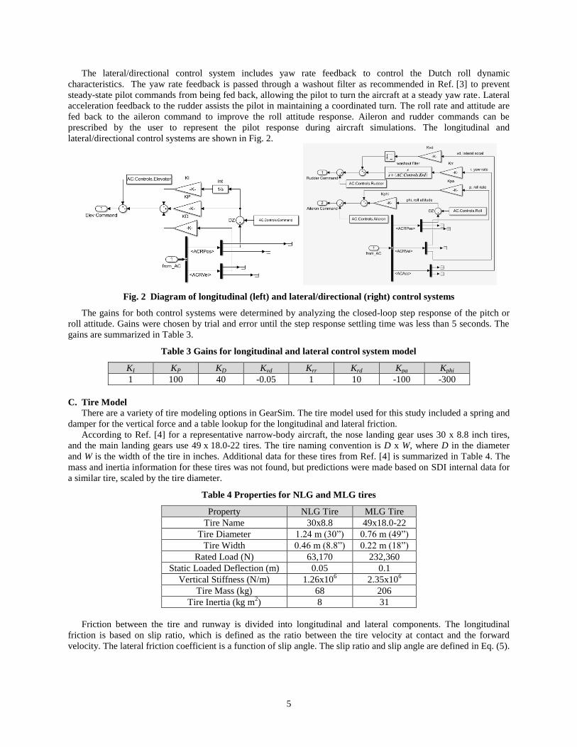
The lateral/directional control system includes yaw rate feedback to control the Dutch roll dynamic

characteristics. The yaw rate feedback is passed through a washout filter as recommended in Ref. [3] to prevent

steady-state pilot commands from being fed back, allowing the pilot to turn the aircraft at a steady yaw rate. Lateral

acceleration feedback to the rudder assists the pilot in maintaining a coordinated turn. The roll rate and attitude are

fed back to the aileron command to improve the roll attitude response. Aileron and rudder commands can be

prescribed by the user to represent the pilot response during aircraft simulations. The longitudinal and

lateral/directional control systems are shown in Fig. 2.

Fig. 2 Diagram of longitudinal (left) and lateral/directional (right) control systems

The gains for both control systems were determined by analyzing the closed-loop step response of the pitch or

roll attitude. Gains were chosen by trial and error until the step response settling time was less than 5 seconds. The

gains are summarized in Table 3.

Table 3 Gains for longitudinal and lateral control system model

KI KP KD Kvd Krr Krd Kpa Kphi

1 100 40 -0.05 1 10 -100 -300

C. Tire Model

There are a variety of tire modeling options in GearSim. The tire model used for this study included a spring and

damper for the vertical force and a table lookup for the longitudinal and lateral friction.

According to Ref. [4] for a representative narrow-body aircraft, the nose landing gear uses 30 x 8.8 inch tires,

and the main landing gears use 49 x 18.0-22 tires. The tire naming convention is D x W, where D in the diameter

and W is the width of the tire in inches. Additional data for these tires from Ref. [4] is summarized in Table 4. The

mass and inertia information for these tires was not found, but predictions were made based on SDI internal data for

a similar tire, scaled by the tire diameter.

Table 4 Properties for NLG and MLG tires

Property NLG Tire MLG Tire

Tire Name 30x8.8 49x18.0-22

Tire Diameter 1.24 m (30”) 0.76 m (49”)

Tire Width 0.46 m (8.8”) 0.22 m (18”)

Rated Load (N) 63,170 232,360

Static Loaded Deflection (m) 0.05 0.1

Vertical Stiffness (N/m) 1.26x106 2.35x10

6

Tire Mass (kg) 68 206

Tire Inertia (kg m2) 8 31

Friction between the tire and runway is divided into longitudinal and lateral components. The longitudinal

friction is based on slip ratio, which is defined as the ratio between the tire velocity at contact and the forward

velocity. The lateral friction coefficient is a function of slip angle. The slip ratio and slip angle are defined in Eq. (5).

6

𝜎 =𝑉𝑥 − Ω𝑟

𝑉𝑥

; tan 𝛼𝑠 = 𝑉𝑦/𝑉𝑥 (5)

The lateral force on the tire and restoring (vertical) moment are then functions of the slip angle. Lookup tables

are used to find the longitudinal friction coefficient based on the slip ratio, the lateral friction coefficient based on

the slip angle, and the restoring moment arm based on the slip angle. For this study, the same relationship was used

for all tires and is plotted in Fig. 3. In practice, if the user has access to accurate longitudinal friction vs. slip ratio

data, or lateral friction and restoring moment vs. slip angle data, this data may be input directly into GearSim.

Fig. 3 Tire friction data for all tires

D. Landing Gear Leg Model

The landing gear leg model can be either rigid or flexible. In the rigid case, the leg model simply transfers forces

and moments from the wheel assembly to the aircraft. In the flexible case, a finite element model is constructed for

the leg. Reference [5] contains several diagrams for a representative nose landing gear (NLG) and main landing gear

(MLG), and these are shown in Fig. 4. The overall dimensions of the landing gear are given in Table 5 and the

landing gear models are shown in Fig. 5. The dimensions given in Table 5 are only a portion of the inputs required

for the flexible leg model; the additional inputs are omitted for brevity.

Fig. 4 Diagrams of A321 NLG and MLG (Ref. [5]) used to find leg dimensions

Table 5 Overall dimensions of NLG and MLG landing gears

Property NLG MLG

Upper tube length (m) 1.375 2.214

Upper tube diameter (m) 0.194 0.2215

Maximum extension of lower tube (m) 0.531 0.6547

Lower tube diameter (m) 0.111 0.18

Wheel lateral separation (m) 0.5 0.928

7

Fig. 5 Pictures of nose, port, and starboard landing gears (left to right)

In the flexible case, a finite element model is generated from a parametric description of the leg. The finite

element model is designed for landing gear that consists of an upper and lower tube, with the lower tube fitting

inside the upper tube. The lower leg contributes to the bending stiffness of the finite element model but not the

torsion. In this example, steel material properties were used to generate the finite element model.

The torque link is modeled as a rotational spring connecting the torsional degree of freedom at the lowest node

of the upper leg with the lowest node of the lower leg. The spring constant is calculated by forming a finite element

model of the torsional spring, and then performing a static Guyan reduction to isolate a single spring constant. The

geometry of the torque link finite element model is dependent upon the closure position, so the torsional spring

constant is also a function of closure position.

E. Oleo/Pneumatic Shock Absorber Model

Modern aircraft typically use oleo/pneumatic shock absorber systems (referred in this work as “oleos”) to absorb

the kinetic energy of the aircraft on landing and provide a comfortable touchdown. Energy absorbed by the oleo can

be calculated by integrating the closure force as a function of travel on compression and subtracting the integral of

closure force as a function of travel on recoil.

The oleo model is a nonlinear mass, spring and damper system. The spring force is a nonlinear function of oleo

closure and corresponds to compression of the gas chamber in the oleo. Reference [1] gives a procedure for

designing the oleo spring force based on the ratio of oleo pressures between the fully compressed and static oleo

closure positions. The procedure is based on a design static load and the final result is the oleo spring force as a

function of oleo closure.

The damping force is a function of fluid flowing through the various orifices in the oleo. As a fluid chamber

closes, fluid flows from one chamber to the next and this creates a pressure difference across the orifice. This

pressure difference is often a function of the fluid velocity squared, with a constant depending upon the fluid

properties and orifice diameters. A metering pin is placed within the main oleo orifice with a non-uniform diameter,

such that the effective orifice diameter changes as a function of oleo stroke. Secondary orifices, with one-way valves

that close during compression and open during rebound, function to change the oleo damping characteristics

depending on the sign of the closure rate. As a result, the oleo has different damping characteristics during

compression and recoil. The oleo damping can be described by the following:

𝐹𝑑𝑎𝑚𝑝𝑖𝑛𝑔(𝑠, 𝑉𝑜𝑙𝑒𝑜) = {𝑐𝑐(𝑠)𝑉𝑜𝑙𝑒𝑜(𝑠)2 𝑉𝑜𝑙𝑒𝑜 > 0

−𝑐𝑟(𝑠)𝑉𝑜𝑙𝑒𝑜(𝑠)2 𝑉𝑜𝑙𝑒𝑜 < 0 (6)

Voleo(s) is the rate of change of the oleo closure at each value of closure. In the absence of data to accurately

describe the oleo, assumptions were made based on Ref. [1] as to the ideal performance of the oleo. With the tire

model, landing gear leg model, design load, and design descent rate, the following assumptions were used to

generate a spring and damping force profile:

1) To maximize the energy absorbed on compression stroke, the total force of the oleo should be constant

during the compression stroke.

2) Assuming a constant total oleo force, and knowing the oleo stroke, the simple dynamics equation:

𝑉𝑓2 = 0 = 𝑉𝑧

2 + 2𝑎𝑑 (7)

8

can be used to determine the required acceleration a; the required constant oleo force is then equal to the

acceleration divided by the effective mass of the aircraft. The effective mass of the aircraft is the design

oleo load divided by g.

3) Oleo damping force is typically designed to be lower at low stroke values, so that the ride is smoother when

taxiing.

Applying assumptions (1) and (2) above, we can find the ideal damping coefficient as a function of oleo stroke:

𝐹𝑖𝑑𝑒𝑎𝑙 = 𝑚𝑎 (𝑉𝑧

2

2𝑑) = 𝐹𝑠𝑝𝑟𝑖𝑛𝑔(𝑠) + 𝐹𝑑𝑎𝑚𝑝𝑖𝑛𝑔(𝑠) = 𝐹𝑠𝑝𝑟𝑖𝑛𝑔(𝑠) + 𝑐(𝑠)𝑉𝑜𝑙𝑒𝑜(𝑠)2 (8)

𝑐(𝑠) =(𝐹𝑖𝑑𝑒𝑎𝑙 − 𝐹𝑠𝑝𝑟𝑖𝑛𝑔(𝑠))

𝑉𝑜𝑙𝑒𝑜(𝑠)2 (9)

An estimate of the closure rate as a function of stroke was found by solving the two degree-of-freedom system

by the aircraft and oleo mass. A free body diagram of this system is shown in Fig. 6, with the aircraft mass shown on

the left with mass ma and the oleo mass shown on the right with mass mo.

Fig. 6 Free body diagram of dynamic system used to design oleo

Assuming the lift force, Flift is equal to the weight of the aircraft mass, the equations of motion and the initial

conditions are given below:

𝑚𝑎�̈�𝑎 = −𝐹𝑜𝑙𝑒𝑜(𝑠, �̇�) (10)

𝑚𝑜�̈�𝑜 = 𝐹𝑜𝑙𝑒𝑜(𝑠, �̇�) − 𝐹𝑡𝑖𝑟𝑒(𝑥𝑜) + 𝑚0𝑔 (11)

where:

𝑠 = 𝑥0 − 𝑥𝑎 (12)

The forces on the oleo and tire are given by:

𝐹𝑜𝑙𝑒𝑜(𝑠, �̇�) = 𝐹𝑠𝑝𝑟𝑖𝑛𝑔(𝑠) + 𝑐(𝑥)�̇�2 (13)

𝐹𝑡𝑖𝑟𝑒 = {𝑘𝑡𝑖𝑟𝑒𝑥0 𝑥0 > 0

0 𝑥0 ≤ 0 (14)

The initial conditions are:

𝑥0(0) = 𝑥𝑎(0) = 0 (15)

�̇�0(0) = �̇�0(0) = 𝑉𝑧 (16)

An iterative process was used to find the ideal damping. First, an initial guess of the damping coefficient 𝑐(𝑠)

was used to generate an initial time history of 𝑠(𝑡). The time histories of oleo closure position and rate 𝑠(𝑡) and �̇�(𝑡)

were combined to form a new estimate of 𝑉𝑜𝑙𝑒𝑜(𝑠)2. Equation (9) above was invoked to calculate the ideal

distribution of 𝑐(𝑠), and a new time history of 𝑠(𝑡) was generated.

9

For the main landing gear, the static oleo force is used as the design load to estimate the spring force profile, and

it is assumed that each main landing gear oleo slows down half of the aircraft mass. Therefore, half of the aircraft

mass is used as the sprung mass. The inputs to the oleo property estimation process for the MLG are shown in Table

6.

For the nose landing gear, the maximum load occurs during maximum braking. Preliminary analysis of the

whole aircraft braking found that the vertical load on the nose landing gear increased to approximately 125,000 N

while braking (the static load is approximately 63,000 N). The majority of the vertical motion of the nose landing

gear is due to aircraft rotation; therefore the aircraft inertia was used to calculate the sprung mass. In the above

analysis, Eq. (11) can be rewritten in terms of rotation, to find an equivalent sprung mass based on the aircraft pitch

inertia and the moment arm between the aircraft CG and the nose landing gear (𝑟𝑁𝐿𝐺):

𝐼𝑦�̈�𝑎𝑟𝑁𝐿𝐺 = 𝐹𝑂𝑙𝑒𝑜𝑟𝑁𝐿𝐺 (17)

(𝐼𝑦

𝑟𝑁𝐿𝐺2 ) �̈�𝑎 = 𝐹𝑂𝑙𝑒𝑜 → 𝑚𝑎 = (

𝐼𝑦

𝑟𝑁𝐿𝐺2 ) (18)

The design force and equivalent mass used to estimate the NLG oleo properties are shown in Table 6.

Table 6 Inputs used to estimate oleo spring and damping force profiles

Oleo Design Parameter NLG MLG

Design Force 125,000 N 356,200 N

Sprung Mass 42,000 kg 37,500 kg

PS / PE 4 4

PC / PS 3 3

Descent Velocity 2 m/s 3 m/s

This procedure typically results in high coefficient values at low and high stroke values. At low stroke values the

spring force is low, so the ideal damping is high, and the velocity is low as the system is just starting to compress. At

high stroke values, the velocity is low as the system is slowing to a stop (before it rebounds). The high damping

values at low stroke values violates the assumption that damping is low during this portion, so the ideal damping

curve was modified to account for this. The result of this procedure for the MLG including both the ideal and

modified damping curves is shown in Fig. 7.

Fig. 7 Ideal and modified damping coefficient used for MLG oleo

Note that this procedure was only conducted in the absence of data to describe the oleo spring and damping

force. In many practical applications, the oleo spring force and damping characteristics can be obtained from

manufacturer’s specifications. In this case, the spring and damping characteristics can be entered into GearSim

directly.

10

F. Braking and Antiskid Model

Braking is an essential part of the landing maneuver and a simple braking analysis is presented in this paper.

GearSim includes two types of braking models: A hydraulic brake pipe model that includes a servo-valve, brake

pipe, and brake fluid accumulator; and a simplified model that applies the braking torque specified by the user. In

both cases, the interaction between the stator (non-rotating part of the brake) and rotor (rotating part of the brake) is

captured with a stick-slip friction model. For this case, the simpler applied-torque braking model was used, as the

focus on this work is not on brake modeling. The simplicity of the applied-torque braking model means an antiskid

system can be designed that functions “perfectly,” keeping the tire at the ideal slip ratio and thus achieving the

maximum possible braking force.

The antiskid model is shown in Fig. 8. It is a PI control system that feeds back aircraft velocity and tire rotational

speed (“AC Vel” and “Omega” in Fig. 8, respectively) to the input braking command. It also includes a rate limiter

with adjustable time constant and positive/negative rate limits.

Fig. 8 Antiskid model used in braking analyses

A summary of the chosen antiskid parameters are given in Table 7. These were chosen using trial and error to

minimize the stopping distance of a similar configuration.

Table 7 Summary of braking and antiskid parameters

Parameter Value

Braking Torque Command 100,000 N-m

Rolling Radius (RRAD) 0.59

Command Gain KC 2x10-6

Proportional Gain KP 1.5x106

Integration Gain KI 2x105

Lead Time Constant (TOR1) 6

Lag Time Constant (TOR2) 1

Positive Rate Limit 1500

Negative Rate Limit 100,000

V. Dynamic Landing Loads

This section demonstrates GearSim’s capability to analyze dynamic landing loads in two scenarios: Symmetric

landing with braking, and asymmetric landing. The first example showcases the landing and braking capabilities of

GearSim and is the baseline landing case used to design landing gear. The second example demonstrates the

crosswind landing capabilities of GearSim.

11

A. Symmetric Landing with Brakes

The simulation of symmetric aircraft landing with braking serves as a baseline case for ground loads analysis and

a means to estimate the loading on the NLG for the purposes of oleo design (see Table 6). This landing simulation

was repeated for rigid and flexible leg models.

The symmetric landing case starts at a trimmed descent rate of 3 m/s; this represents the aircraft motion just after

the flare maneuver is conducted and represents a higher-than-average rate of descent. The trim pitch angle is 4.7

degrees in this case. After the main landing gears touch down, the pitch attitude command is changed linearly from

4.7 degrees to -1.5 degrees over the time period between 1 s and 2 s. At 5 seconds into the simulation, the braking

demand is applied to both main landing gears for 10 seconds, for a total simulation duration of 15 seconds.

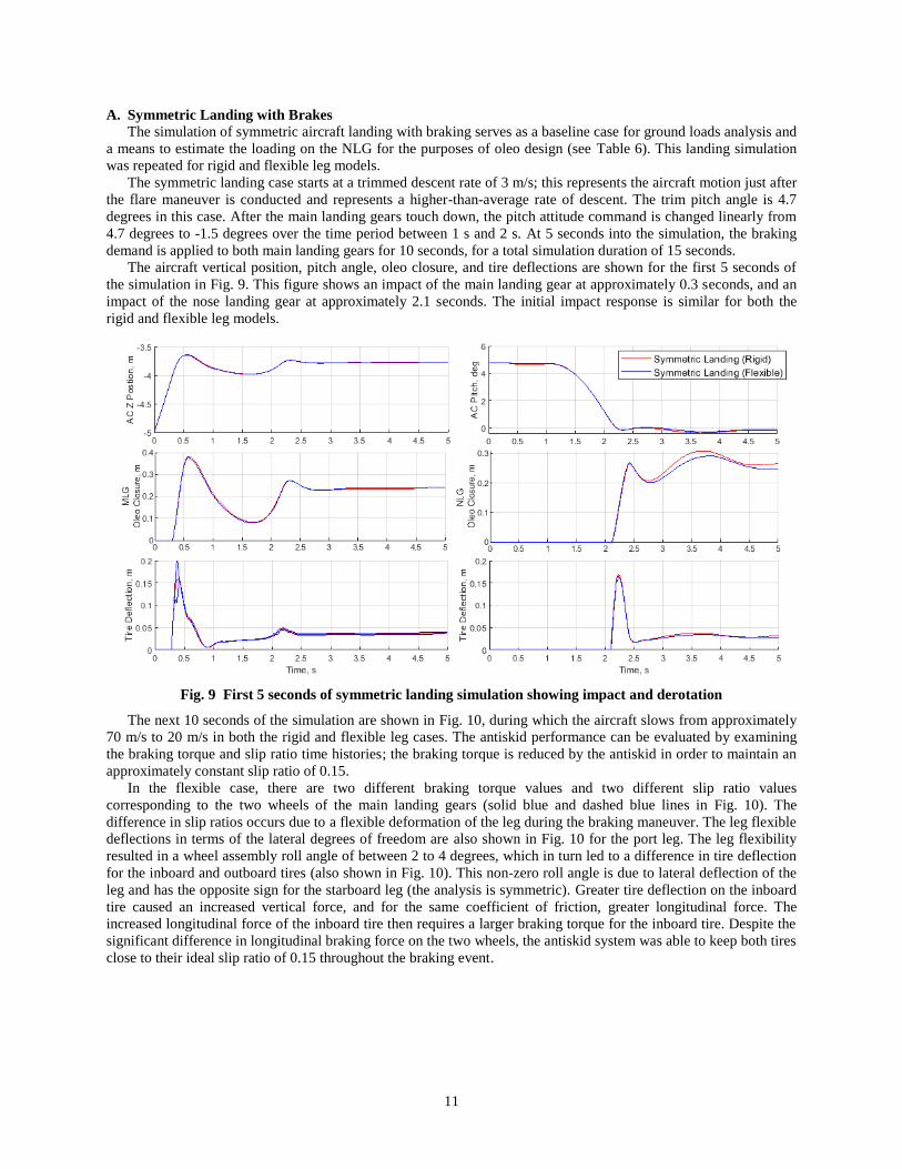
The aircraft vertical position, pitch angle, oleo closure, and tire deflections are shown for the first 5 seconds of

the simulation in Fig. 9. This figure shows an impact of the main landing gear at approximately 0.3 seconds, and an

impact of the nose landing gear at approximately 2.1 seconds. The initial impact response is similar for both the

rigid and flexible leg models.

Fig. 9 First 5 seconds of symmetric landing simulation showing impact and derotation

The next 10 seconds of the simulation are shown in Fig. 10, during which the aircraft slows from approximately

70 m/s to 20 m/s in both the rigid and flexible leg cases. The antiskid performance can be evaluated by examining

the braking torque and slip ratio time histories; the braking torque is reduced by the antiskid in order to maintain an

approximately constant slip ratio of 0.15.

In the flexible case, there are two different braking torque values and two different slip ratio values

corresponding to the two wheels of the main landing gears (solid blue and dashed blue lines in Fig. 10). The

difference in slip ratios occurs due to a flexible deformation of the leg during the braking maneuver. The leg flexible

deflections in terms of the lateral degrees of freedom are also shown in Fig. 10 for the port leg. The leg flexibility

resulted in a wheel assembly roll angle of between 2 to 4 degrees, which in turn led to a difference in tire deflection

for the inboard and outboard tires (also shown in Fig. 10). This non-zero roll angle is due to lateral deflection of the

leg and has the opposite sign for the starboard leg (the analysis is symmetric). Greater tire deflection on the inboard

tire caused an increased vertical force, and for the same coefficient of friction, greater longitudinal force. The

increased longitudinal force of the inboard tire then requires a larger braking torque for the inboard tire. Despite the

significant difference in longitudinal braking force on the two wheels, the antiskid system was able to keep both tires

close to their ideal slip ratio of 0.15 throughout the braking event.

12

Fig. 10 Aircraft and landing gear response during symmetric landing with brakes case

The forces on the nose and main landing gears for this case are shown in Fig. 11. These show a negligible

difference between the rigid and flexible cases during the initial impact. However, there are significant differences

between the rigid and flexible cases during the braking portion of the simulation. Fig. 11 shows a decrease in the

nose leg force in the z-direction for the flexible case compared to the rigid case, and again this decrease is due to the

flexible deflections of the leg during the braking maneuver. The value of 125,000 N used to design the nose landing

gear oleo was derived from Fig. 11 for the rigid case. The forces on the main landing gear show very similar loading

between the rigid and flexible case, with the biggest difference being a non-zero force in the y-direction for the

flexible case during the braking portion of the simulation. This is due to the yaw angle of the tire (resulting from leg

flexibility), which results in a non-zero lateral coefficient of friction and side force from the tire.

13

Fig. 11 Leg forces during symmetric landing with braking case

B. Asymmetric Landing with Crosswind

GearSim can be used to analyze the dynamic loads for a variety of landing scenarios. One scenario of interest is

landing in a crosswind. In general, there are three approach patterns that can be followed in this case. The first,

known as “crab,” involves aligning the aircraft with the wind direction and landing at a yaw angle. After touchdown,

the pilot applies rudder and aileron commands as necessary to straighten out the aircraft. The second, known as “de-

crab,” approaches the runway aligned with the wind direction, but the pilot applies rudder and aileron commands

just before touchdown to straighten out the aircraft. The third approach pattern is known as “sideslip,” and in this

pattern the pilot will approach the runway aligned with the runway centerline, but with non-zero roll attitude and

non-zero rudder and aileron settings.

For commercial aircraft, the “crab” and “de-crab” approaches are generally preferred to the “sideslip” approach,

because with “sideslip” the non-zero roll attitude can reduce ground clearance, especially for wing-mounted engines.

The “crab” approach leads to significant runway deviation due to the lateral forces acting on the tires, and therefore

is not recommended for dry runway surfaces. For wet runway surfaces, the runway deviation due to the lateral

friction will be reduced and the “crab” approach may be used to reduce the pilot workload.

For this paper, a crosswind velocity of 10 m/s will be used. According to Ref. [6], the maximum crosswind

velocity at landing for an A320 is around 33 kts or 16 m/s, so 10 m/s is a large crosswind velocity but within the

operational capabilities of this class of aircraft. GearSim has a built in trim feature to enable analysis of the different

maneuvers. Table 8 summarizes the trim conditions for the different approach patterns.

14

Table 8 Trim conditions for different approach patterns

Trim Variable Crab / De-crab Sideslip

Crosswind Velocity (m/s) 10 10

Sink Rate (m/s) 3 3

Ground Speed (m/s) 75 75

Thrust (N) 32,000 37,550

Roll Attitude (deg) 0 -3.8

Pitch Attitude (deg) 4.5 5.0

Yaw Attitude (deg) -7.6 0

Elevator Setting (deg) -6 -6.5

Rudder Setting (deg) 0 -13

Aileron Setting (deg) 0 -36

Simulations of landing in the crab, de-crab, and sideslip approach patterns were conducted for a duration of 10

seconds. In all cases, the initial pitch attitude command was set to the trim approach attitude (Table 8) from 0 to 4

seconds, reduced to -2 degrees from 4 to 6 seconds, and held at -2 degrees for the remainder of the simulation. Trial

and error was used to find the appropriate time history of rudder commands that would align the aircraft with the

runway in the crab and de-crab cases. The aircraft position for each case is shown in Fig. 12, the oleo closure time

histories are shown in Fig. 13 and the elevator, aileron, and rudder commands are shown in Fig. 14.

The aircraft position and oleo closure time histories (Fig. 12 and Fig. 13) indicate that the main landing gear

impacts at around 2 seconds, and the derotation occurs from 2 to 4 seconds, with impact on the nose landing gear

occurring at around 5.6 seconds. Fig. 13 shows that for the crab and de-crab cases, both main landing gears impact

at the same time, but for the sideslip case, the port landing gear impacts first.

The aircraft position and control setting time histories (Fig. 12 and Fig. 14) show that for both the crab and de-

crab cases, the rudder commands were sufficient to reorient the aircraft along the runway centerline (yaw angle of

zero). In the de-crab case, the pilot begins the rudder command to reorient the aircraft at the beginning of the

simulation, so that the aircraft lands at around -4 degrees yaw instead of -7.6 degrees in the crab case. The higher

yaw angle at impact for the crab case led to a deviation from the runways centerline of 20 m in the crab case,

compared to only 8 m deviation in the de-crab case.

Fig. 12 Aircraft position and orientation angles for asymmetric landing simulations

15

Fig. 13 Oleo closure time histories for asymmetric landing simulations

Fig. 14 Elevator, rudder, and aileron deflections for asymmetric landing simulations

The leg force results from the asymmetric landing simulation are shown in Fig. 15. These show very similar vertical

force results for both crab and de-crab scenarios, but larger y-forces for the crab scenario due to the higher yaw

angle on impact. In the sideslip case, the port landing gear impacts before the starboard landing gear. This leads to

much lower forces on the starboard leg during this scenario; the vertical force on the starboard gear is almost 60%

lower than in the crab and de-crab cases. The peak vertical force on the port leg was slightly higher for the sideslip

case (710 kN in the sideslip case compared to 630 kN in the crab case).

16

Fig. 15 Leg forces for asymmetric landing simulations

VI. Conclusion

This paper introduces GearSim as a dynamic analysis tool for landing gear. GearSim is ideal for analyzing the

dynamic response of landing gear and determining the loads that the airframe and the gear itself will experience

during complicated takeoff, landing, and ground maneuver scenarios. The scenarios presented in this paper are a few

examples of the broad capabilities that GearSim has to offer in terms of landing gear and ground loads analysis.

The next step in demonstrating the dynamic loads analysis capability of GearSim will be to include the effects of

aircraft flexibility into the analysis. Aircraft flexibility can be introduced by developing an aeroelastic model of the

airframe in Nastran. GearSim can then import the structural and aerodynamic matrices from Nastran and simulate

the airframe flexibility along with the landing gear dynamics. Simulations including aeroelasticity can then be post-

processed to find the airframe loads during takeoff, landing, and ground maneuvers.

Future work will attempt to determine the influence of the landing condition on the ground loads by applying a

Monte-Carlo approach to simulate the landing event in a variety of different landing conditions. The Monte Carlo

approach will also be used to quantify uncertainty in the ground loads results with respect to uncertainty in the

modeling parameters. Statistical analysis of the ground loads results will then give insight into the possible variation

of maximum loads and loading profile for typical aircraft operations.

A sensitivity analysis of the GearSim models can also be useful to determine the parameters that most impact the

dynamic characteristics of the landing loads. This will be performed by varying key parameters in the model, such

as tire vertical stiffness, landing gear structural properties, or oleo performance characteristics to find the effect on

the maximum vertical load. Initial work has revealed the tire, oleo and the flight control system to be the most vital

subsystems with respect to the dynamic landing loads analysis.

Longitudinal and lateral vibrations of the landing gear were present in the flexible braking case shown, albeit

highly damped. These vibrations are due to the leg flexibility and in certain situations can become lightly damped or

even unstable. Interaction between the longitudinal leg flexibility and the braking and antiskid system is often

referred to as gear walk, and interaction between the lateral leg flexibility and tire lateral and yaw forces is often

referred to as shimmy. Further work will use GearSim to characterize these vibrations by analyzing the parameters

that have the largest impact on the frequency, damping, and stability.

Acknowledgments

SDI Engineering would like to thank LGTF for their support of the GearSim development and validation effort

through the SBIR program. This material is based upon work supported by the United States Air Force under

contract award FA2487-16-C-0085 to SDI Engineering Inc. Any opinions, findings, and conclusions or

recommendations expressed in this publication are those of the author(s) and do not necessarily reflect the views of

the United States Air Force or SDI Engineering Inc.

17

SDI Engineering would like to thank Airbus Americas Inc., especially David Hills and Amanda Simpson, for

their support of the GearSim development and validation.

Phillip W. Richards would like to thank Cole Morgan and Max McDonald for their assistance in setting up the

crosswind landings cases and gathering detailed landing gear geometry data.

Disclaimer: "This report was prepared as an account of work sponsored by an agency of the United States

Government. Neither the United States Government nor any agency thereof, nor any of their employees, makes any

warranty, express or implied, or assumes any legal liability or responsibility for the accuracy, completeness, or

usefulness of any information, apparatus, product, or process disclosed, or represents that its use would not infringe

privately owned rights. Reference herein to any specific commercial product, process, or service by trade name,

trademark, manufacturer, or otherwise does not necessarily constitute or imply its endorsement, recommendation, or

favoring by the United States Government or any agency thereof. The views and opinions of authors expressed

herein do not necessarily state or reflect those of the United States Government or any agency thereof."

References

[1] Currey, N. S., Aircraft Landing Gear Design, Principles and Practices. American Institute of Aeronautics

and Astronautics, Inc. 1988.

[2] Airbus, “A321neo: The most efficient single-aisle jetliner.” URL:

https://www.airbus.com/aircraft/passenger-aircraft/a320-family/a321neo.html. [retrieved 24 October 2006].

[3] Blakelock, John H., Automatic Control of Aircraft and Missiles, J. Wiley and Sons, 1991.

[4] Goodyear Aviation, “Global Aviation Tires” Aircraft Tire Databook. URL:

https://www.goodyearaviation.com/resources/pdf/databook-6-2018.pdf [retrieved 24 October 2006].

[5] Airbus S.A.S., “A321: Aircraft Characteristics Airport and Maintenance Planning.” Airbus S.A.S.,

Technical Data Support and Services. Issue: 30 September 1992. Updated: 1 February 2018.

[6] Zagoren, Matt., “Airbus A320-232 Limitations (IAE V2527-A5).” SATA-Azores Airlines Fleet Data.

URL: http://www.satavirtual.org/fleet/A320LIMITATIONS.PDF [retrieved 11/1 2006].