Discussion Paper No.132

A Theory of Multiperiod Financial Contracts that do not

Balance the Budget

Mamiko Terasaki

May 2010

GCOE Secretariat Graduate School of Economics

OSAKA UNIVERSITY 1-7 Machikaneyama, Toyonaka, Osaka, 560-0043, Japan

GCOE Discussion Paper Series

Global COE Program Human Behavior and Socioeconomic Dynamics

A Theory of Multiperiod Financial Contracts that do not

Balance the Budget

Mamiko Terasaki∗ †

Kyoto University

Abstract

This paper seeks financial contracts that specify a repayment schedule that in-

duces both the investor and the entrepreneur to contribute to the project when the

entrepreneur privately observes the realizations. Any optimal contracts do not bal-

ance the budget, i.e., some amount of money must be transferred to or from a third

party depending on the history of the output realizations. We specify multiperiod

optimal contracts not only with budget feasibility constraint but also without it and

explain venture capital contracts as an example of the contracts that expect a third

party to break the budget without budget feasibility constraint.

JEL Classifications: D82, D86, G20, G24, G30

Keywords: financial contract, budget-breaking, and venture capital.

∗Email: mamiko.terasaki@gmail.com.†I would like to thank Hiroshi Osano, Akihisa Shibata, and Tadashi Sekiguchi for continuous guidance

and support.

1

1 Introduction

In the case in which a project’s output realizations can be observed only by an en-

trepreneur, a repayment must be independent of the realizations for the entrepreneur

to truthfully report them. However, an investor and an entrepreneur must obtain pay-

offs that are dependent on the realizations to induce them to contribute to the project.

Therefore any efficient contracts do not balance the budget, i.e., the amount the en-

trepreneur repays is different from the amount the investor obtains under some con-

ditions. Players use a third party to differentiate between these two amounts. With

budget feasibility constraint, i.e., the assumption that the amount the entrepreneur re-

pays must be larger than the amount the investor obtains, the third party must receive

some amount of money from the players to differentiate between two amounts. However

in the real world, we do not need to assume budget feasibility; for example, venture

capitalists and venture firms expect general investors to provide money for them if their

projects succeed by buying venture firms’ shares through initial public offerings.

This paper discusses financial contracts between an entrepreneur and an investor.

The contract specifies a repayment schedule that depends on the history of the output

realizations. Here, we assume that the entrepreneur can observe the realizations but the

investor cannot do so. We also assume that neither the investor nor the entrepreneur can

commit their contributions to the project every period. It is possible for the investor to

decrease the quality his financial services or for the entrepreneur to lower her effort level,

2

either of which would lower the probability that the project succeeds. Furthermore, since

it is also possible for the entrepreneur to lie about the project’s realization, the investor

may be unwilling to contribute to the project.

We can find these kinds of financial contracts in the real world. First, one can deposit

money in money management companies and later obtain a return based on performance.

Second, under Mudarabah, one of the basic forms of Islamic banking, a bank and an

entrepreneur share a project’s profits or losses according to a predetermined ratio. In

both cases, investors or depositors can choose the amount of money they contribute in

each period and their continuous contributions are important to the borrowers’ projects.

Moreover, in neither case can investors or depositors directly observe the performance

or output realization of projects, so borrowers may lie about them to increase their own

payoffs.

Townsend (1979), Diamond (1984), and Gale and Hellwig (1985) analyze the situa-

tion that lenders cannot observe the project’s outputs without paying a finite monitoring

cost. To induce the borrower to be honest about the output realization, the lender must

audit the borrower and deprive the borrower of all of the output realizations when the

borrower reports poor performance. In contrast, we assume that the monitoring costs

are infinitely high. Bolton and Scharfstein (1990) also analyze this case and propose that

financial institutions must stop lending in the second period with a positive probability

when the borrower reports poor performance at the end of the first period to induce

them to truthfully send messages about a project’s performance. However, they fail to

3

give the borrower any incentive to be truthful in the last period.

This paper models the case where both entrepreneur’s contribution and an investor’s

contribution are important to the project. The model is similar to the ones that study

moral hazard in teams (Holmstrom(1982)) and double-sided moral hazard in franchise

contracts (Bhattacharyya and Lafontaine(1995)). They assume that all players can

observe project’s output realizations but we analyze the situation that an entrepreneur

can observe the realizations but an investor cannot do so. Holmstrom(1982) shows that

noncooperative behavior by players always yields an inefficient result when joint output

realization is fully shared among them and that they can make an efficient contract when

the sum of the amounts shared among players can be more or less than the joint output

realization, i.e., when a third party breaks the budget by seizing a part of the realization

from players or by paying them a bonus.

Recently, MacLeod (2003) and Kambe (2006) discussed an agency contract when a

principal privately observes an agent’s output realizations. To induce the agent to exert

effort and the principal to be truthful about the realizations, the wage the principal pays

and that the agent receives must be different under some conditions. Since they assume

budget feasibility, i.e., the amount the principal pays must be larger than the amount the

agent obtains, the differentiated amount of money must be passed to a third party. Here,

a third party again plays a role in breaking the budget. Fuchs (2007) proposes a method

to reduce the amount to be passed to a third party in a repeated game setting. We apply

their findings to a financial contract under which a principal’s effort level also affects the

4

project’s output realizations. Although they assume budget feasibility constraint, we

also seek optimal financial contracts without this constraint because financial contracts

that count on a third party to pay exist in the real world.

For the entrepreneur to truthfully report output realizations to the investor, the

amount she repays must be independent of the output realizations. However, to induce

players to contribute to the project, the payoffs the investor and the entrepreneur obtain

after the projects must be dependent on the output realizations. Since repayment must

always be constant, it is the project’s property that gives the entrepreneur an incentive

to make a high level of effort. In other words, the project must be likely to generate

high enough output realization when the entrepreneur exerts a high level of effort and

low enough when she exerts a low level of effort. On the other hand, it is the transfer

to or from the third party that gives the investor an incentive to provide good financial

services in each period.

The advantage of multiperiod contract in this paper is to reduce the discounted

expected amount of money to be transferred to or from the third party. When the en-

trepreneur hides information on the output realizations until the end of the relationship,

the contracts that give players good incentives in the first period also can give them

good incentives in the succeeding period. When we assume budget feasibility constraint,

the optimal contract, which minimizes the discounted expected amount of the transfer

to the third party, requires no amount of the transfer if the output realization in the

first period is high regardless of the realization in the succeeding period.

5

Without budget feasibility constraint and with a rational third party, the optimal

contract is the one that minimizes the discounted expected amount of the transfer from

the third party and that requires no amount of the transfer if the realization in the

first period is low regardless of the realization in the succeeding period. A venture

capital contract, under which an investor provides funds and management advice to an

entrepreneur by purchasing convertible securities issued by the entrepreneur, is a good

example of this type of budget-breaking financial contracts in that an venture capitalist

and a venture firm expect a third party to pay for them if their project succeeds.

The remainder of the paper is organized as follows. The next section presents the

general model framework. In section 3, we analyze one-period financial contract with

budget feasibility constraint and the inefficiency of asymmetric information on output

realizations. The first half of Section 4 considers multiperiod contract with budget fea-

sibility constraint and illustrate the way of reducing the inefficiency of budget-breaking.

In the last half of the section, we seek multiperiod contract without budget feasibility

constraint and explain venture capital contracts as an example of this type of budget-

breaking contracts in the real world. Section 5 concludes. All the proofs are contained

in the Appendix.

6

2 The Model

There are two risk-neutral players, an entrepreneur and an investor. The entrepreneur

has a project that stochastically generates outputs, but she does not have funds for it.

The entrepreneur has to finance the project from the investor, who can provide a variety

of financial services in each period. The investor contributes to the project by providing

sound financial and management assistance, but not all of it can be specified in a con-

tract. The entrepreneur and the investor agree on a repayment schedule that depends

on the project’s output realization. The entrepreneur can observe the output realiza-

tion, but the investor cannot. Therefore, the investor is worried that the entrepreneur

may lie about the output realization. In turn, the entrepreneur is concerned that the

investor may reduce his contribution to the project. The investor is also worried that

the entrepreneur may shirk his responsibilities while carrying out the project because

the investor cannot observe the entrepreneur’s effort level.

The entrepreneur and the investor meet at the beginning of period 0, agree to coop-

erate on the project until the end of period T ∈ {0, 1}, and sign a contract that specifies

the repayment schedule.

After signing the contract, the investor chooses his contribution to the project, It ∈

{IH , IL}, at the beginning of each period. Then the entrepreneur chooses her effort

level, et ∈ {eH , eL}. We assume that contributing to the project costs them It and et,

respectively. We also assume that IH > IL and eH > eL. After the project generates

7

output realization yt, the entrepreneur sends a message about it mt(yt). The message

is observable and verifiable. Depending on the message, the entrepreneur repays part of

the output realization, and the investor receives money as specified in the contract.

The output realization is also binary, yt ∈ {yH , yL}, stochastic, and depends on both

the amount of funds and the level of effort. We assume that the project generates yH

with probability p(It, et) and yL with probability 1 − p(It, et). We define the expected

output levels as ysv = E(yt|It = Is, et = ev) = psvyH + (1− psv)yL, where psv ≡ p(It, et |

It = Is, et = ev) for s ∈ {H, L} and v ∈ {H,L}.

We assume that a riskless bond exists in the economy. When a player buys the

riskless bond at the beginning of each period, he will get the same amount of the money

at the end of the same period. We assume the interest rate of this bond is r; when player

buys x worth of this bond in period 0, he will get money worth (1 + r)x in period 1.

Moreover, we have the following assumptions.

Assumptions

(a) yHH > yLH and yHH > yHL

(b) yHH − IH − eH > yLH − IL − eH > 0

(c) yHH − IH − eH > yHL − IH − eL

(d) yLH − IL − eH < yLL − IL − eL

Assumption (a) implies that p(It, et) is an increasing function of both It and et. In

other words, the more funds the investor lends, the more likely the project will succeed.

8

Similarly, the more effort the entrepreneur exerts, the more likely the project will succeed.

Assumption (b) means that, given that the entrepreneur exerts a high level of effort,

more funds are more efficient than fewer funds, and fewer funds are more efficient than

riskless bonds. Assumption (c) implies that, given that the investor lends a large amount

of money, a high level of effort is more efficient than a low level. On the other hand,

assumption (d) denotes that, given that the investor lends a small amount, a low level

of effort is more efficient than a high level. It also means that the increase of the

expected output realizations by intensifying the entrepreneur’s effort level is lower than

the increase of effort costs by doing so when the investor lends a small amount of money.

These assumptions imply that the project’s expected output realization is maximized

if and only if both players contribute to the project. We refer to a contract under which

the project’s expected output realizations are maximized as an efficient contract. In

this paper, the entrepreneur offers a contract that maximizes her own expected payoff

as well as maximizes the project’s expected outputs. We call such a contract an optimal

contract. An optimal contract is always efficient, but an efficient contract is not neces-

sarily optimal. We also define the following expressions: ∆y ≡ yH − yL, ∆I ≡ IH − IL,

∆e ≡ eH − eL, ∆p(I) ≡ pHH − pLH , and ∆p(e) ≡ pHH − pHL. Note that all of these

expressions are nonnegative.

9

3 One-Period Contract

In this section, we discuss the case in which the project generates output only once:

when T = 0. When the output realizations are observed by both players, the contracts

can specify the repayment that depends on them. However, when the output realizations

are only observed by the entrepreneur, the repayment can no longer depend on them.

3.1 Efficient and optimal contracts when output realizations are public

information

To examine the effect of asymmetric information on output realizations, y0, we first

discuss efficient contracts when both the player and the third party observe the project’s

realizations 1. In this case, we can write contracts that depend on the output realizations

and assume that the entrepreneur repays rb ∈ {rbH , rb

L}, i.e., rbH if the output realization

is yH and rbL if it is yL. Similarly, the investor receives rℓ ∈ {rℓ

H , rℓL}, i.e., rℓ

H if the

output realization is yH and rℓL if it is yL. In this section, we assume that rb

H ≥ rℓH and

rbL ≥ rℓ

L. These constraints correspond to budget feasibility constraints in the context of

mechanism design2. If rbH = rℓ

H and rbL = rℓ

L, the amount the entrepreneur repays and

the amount the investor receives are the same, and we say that the contract balances

the budget. If either rbH > rℓ

H or rbL > rℓ

L, we say that the contract does not balance the

1If players can observe the output realization but any third party cannot, the realization cannot be

verifiable in court. Here we assume that output realizations are observable and verifiable.2In section 4.2, we consider the case of rb

H ≤ rℓH and rb

L ≤ rℓL, in which a third party provides money

for players.

10

budget and interpret that the difference between the amount the entrepreneur repays

and the amount the investor receives is passed to a third party. We postulate that both

players are reluctant to transfer any hard-won value to a third party. We denote the

difference of the amount the entrepreneur repays as ∆rb ≡ rbH − rb

L and the difference

of the amount the investor receives as ∆rℓ ≡ rℓH − rℓ

L. Next, we discuss the constraints

that efficient contracts must satisfy and the conditions under which efficient contracts

exist.

First of all, any efficient contracts must guarantee expected payoffs that exceed the

player’s burdens, or guarantee nonnegative net expected payoffs. The entrepreneur

writes and offers the contracts if and only if the expected payoff that she obtains by

exerting effort eH for the project is higher than or identical to her effort costs. Simi-

larly, the investor signs the contract if and only if the expected payoff that he receives

by investing IH is higher than or identical to the payoff that he receives by investing

the same amount of money into riskless bonds. Therefore, any efficient contracts must

satisfy the following constraints:

E(rℓ|I0 = IH , e0 = eH) ≥ IH , (1)

E(y0 − rb|I0 = IH , e0 = eH) ≥ eH . (2)

We refer to constraints (1) and (2) as individual rationality constraints for the investor

and for the entrepreneur respectively. These constraints can be rewritten in the following

11

way:

pHHrℓH + (1 − pHH)rℓ

L ≥ IH , (3)

pHH(yH − rbH) + (1 − pHH)(yL − rb

L) ≥ eH . (4)

In addition to individual rationality constraints, any efficient contract must satisfy

constraints that induce players to greatly contribute to the project:

E(rℓ|I0 = IH , e0 = eH) − IH ≥ E(rℓ|I0 = IL, e0 = eH) − IL, (5)

E(y0 − rb|I0 = IH , e0 = eH) − eH ≥ E(y0 − rb|I0 = IH , e0 = eL) − eL. (6)

The left-hand side of each inequity is each player’s net expected payoff when he greatly

contributes to the project, and the right-hand side is that when he do not so, given that

the other player greatly contributes to the project. We refer to constraints (5) and (6) as

incentive compatibility constraints for the investor and for the entrepreneur respectively.

When both players can observe the project’s output realizations, these constraints can

be rewritten with difference expressions in the following way:

∆rℓ ≥ ∆I

∆p(I)(7)

∆rb ≤ ∆y − ∆e

∆p(e). (8)

Thus, we have the following lemma about the existence of efficient contracts when

both players can observe the project’s output realizations.

Lemma 1 (i) If ∆y ≥ ∆I/∆p(I) + ∆e/∆p(e), there exists an efficient contract that

balances the budget. An efficient contract specifies a repayment schedule such that rbH =

12

rℓH and rb

L = rℓL; thus, no amount of money is transferred to the third party.

(ii) If ∆y < ∆I/∆p(I)+∆e/∆p(e) and yH ≥ IH+eH+(1−pHH) (∆I/∆p(I) + ∆e/∆p(e)),

there are no efficient contracts that balance the budget, but there is an efficient con-

tract that does not balance the budget. The efficient contract that minimizes the trans-

fer to the third party specifies a repayment schedule such that rbH = rℓ

H and rbL =

rℓL+(∆I/∆p(I) + ∆e/∆p(e) − ∆y). In the case of y0 = yL, players transfer ∆I/∆p(I)+

∆e/∆p(e) − ∆y to the third party, i.e., the ex ante expected transfer to the third party

is (1 − pHH)(∆I/∆p(I) + ∆e/∆p(e) − ∆y).

(iii) If ∆y < ∆I/∆p(I)+∆e/∆p(e) and yH < eH+IH+(1−pHH) (∆I/∆p(I) + ∆e/∆p(e)),

there are no efficient contracts.

The case of (i) implies that, when the difference of output realizations between high

and low is large enough, players can make efficient contracts under which they do not

need to transfer any amount of money to a third party. When this difference is small,

an efficient contract has to make a large enough difference by transferring some money

to a third party. However, this transfer reduces the players’ expected payoffs. Thus,

when yH is small, players cannot make contracts that satisfy the individual rationality

constraints for them.

The efficient contract that minimizes the transfer to the third party requires the

following rules. If the output realization is high, the amount of money paid by the

entrepreneur is directly passed to the investor. However, if it is low, the amount of

13

money paid by the entrepreneur must be divided into two parts; one is passed to the

investor and the other to the third party.

It is impossible for these players to negotiate and share the amount to be transferred

to a third party because this renegotiation increases the investor’s payoff when the output

realization is low and violates the incentive compatibility constraint for the investor.

The entrepreneur writes and offers contracts that not only satisfy all these constraints

but also maximize her own expected payoff. We obtain an optimal contract without

asymmetric information on output realizations as follows.

Proposition 1 Suppose that both players and a third party can observe project’s output

realization y0 ∈ {yH , yL} and the contract specifies repayment schedule (rbH , rb

L, rℓH , rℓ

L)

that depends on project’s output realization y0.

(i) If ∆y > ∆I/∆p(I) + ∆e/∆p(e), optimal contracts exist infinitely. Under any

optimal contracts, the investor’s expected payoff is IH , and the entrepreneur’s is yHH −

IH . The optimal contract that binds the incentive compatibility constraint for the investor

specifies a repayment schedule such that

rbH = rℓ

H = IH + (1 − pHH)∆I

∆p(I),

rbL = rℓ

L = IH − pHH∆I

∆p(I).

(ii) If ∆y ≤ ∆I/∆p(I)+∆e/∆p(e) and yH ≥ IH+eH+(1−pHH) (∆I/∆p(I) + ∆e/∆p(e)),

an optimal contract exists and it is unique. The investor’s expected payoff is IH , and

14

the entrepreneur’s is yHH −IH − (1−pHH) (∆I/∆p(I) + ∆e/∆p(e) − ∆y). The optimal

contract specifies a repayment schedule such that

rbH = rℓ

H = IH + (1 − pHH)∆I

∆p(I),

rbL = IH + (1 − pHH)

∆I

∆p(I)+

∆e

∆p(e)− ∆y,

rℓL = IH − pHH

∆I

∆p(I).

For y0 = yL, the amount of ∆I/∆p(I) + ∆e/∆p(e)−∆y is transferred to a third party,

i.e., the ex ante expected transfer to the third party is (1−pHH)(∆I/∆p(I)+∆e/∆p(e)−

∆y).

Proposition 1 provides two types of optimal contracts and the conditions under which

they exist. When ∆y is large, that is, when the difference between a large output

realization and a low one is large, players can make optimal contracts that provide

good incentives for them without transferring any money to a third party. Since players

are risk-neutral, they are indifferent to contracts that give constant expected payoffs.

Therefore, optimal contracts exist infinitely. Among these optimal contracts, the one

that binds the incentive compatibility constraint for the investor is unique. When ∆y is

small but yH is large, players can make a unique optimal contract; however, the budget

won’t balance.

The investor’s expected payoff is always IH . However, the entrepreneur’s expected

payoff varies depending on the project’s property. When players must transfer money

15

to a third party, the contract charges the entrepreneur this amount since the investor

always receives, at most, the same amount of burden. When both ∆y and yH are small,

players cannot make any efficient contracts by Lemma 1, nor can they make any optimal

contracts.

The optimal contracts expressed in Proposition 1 depend on the assumption that both

the players and the third party can observe the project’s output realization. If neither

the investor nor the third party can observe the output realizations, the entrepreneur

may lie about the project’s output realization to increase her own payoff. In the next

section, we discuss efficient and optimal contracts when there is asymmetric information

on the project’s output realizations.

3.2 The efficient and optimal contracts when output realizations are

private information

Suppose that neither an investor nor a third party can observe the output realizations,

but the messages sent by the entrepreneur are observable and verifiable. In this case,

the contract specifies a repayment schedule that depends on those messages. First we

consider a case in which the contracts balance the budget. Then, if rbH > rb

L, i.e.,

∆rb > 0, the entrepreneur always sends message m0(y0) = yL and repays rbL regardless

whether yH or yL is achieved. This is because the entrepreneur can increase her payoff

by minimizing the repayment. However, if the investor anticipates the entrepreneur’s

behavior, he always lends IL. The reason is that the investor’s payoff is rbL−IH if he lends

16

IH and rbL − IL if he lends IL; thus, the latter is always larger than the former. Given

that the entrepreneur always repays rbL, then the contract cannot satisfy the incentive

compatibility constraint for the entrepreneur, since we have

yHL − rbL − eH < yLL − rb

L − eL

by assumption (d).

In contrast, if ∆rb < 0, the entrepreneur always sends message m0(y0) = yH , and

the investor always lends IL. As a result, the necessary and sufficient condition for the

entrepreneur to be honest about the project’s output realization is ∆rb = 0. This con-

straint is equivalent to ∆rℓ = 0 because we are now considering a contract that balances

the budget. However, by constraint (7), ∆rℓ = 0 violates the incentive compatibility

constraint for the investor. Therefore, no contract can balance the budget when there is

asymmetric information on output realization. Consider the following proposition.

Proposition 2 Suppose that neither the players nor the third party can observe project’s

output realization y0 ∈ {yH , yL} and the contract specifies repayment schedule (rbH , rb

L, rℓH , rℓ

L)

that depends on message m0 ∈ {yH , yL}.

(i)No efficient contract balances the budget.

(ii)If yHH ≥ eH + IH + (1 − pHH)∆I/∆p(I) and yL ≥ IH + (1 − pHH)∆I/∆p(I),

there is efficient contracts that do not balance the budget. The unique optimal contract

17

specifies a repayment schedule such that

rbH = rb

L = rℓH =IH + (1 − pHH)

∆I

∆p(I),

rℓL =IH − pHH

∆I

∆p(I).

For m0 = yL, players transfer ∆I/∆p(I) to the third party, i.e., the ex ante expected

amount of the transfer is (1−pHH)∆I/∆p(I). The investor’s expected payoff is IH , and

the entrepreneur’s is yHH − IH − (1 − pHH)∆I/∆p(I).

(iii)If either yHH < eH +IH +(1−pHH)∆I/∆p(I) or yL ≥ IH +(1−pHH)∆I/∆p(I),

there are no efficient contracts.

Compared to Proposition 1, when output realizations are unobservable, players can-

not make any efficient contract that balances the budget. The reason is that the en-

trepreneur will not truthfully send a message without requiring the amount she repays

to be constant, and the investor will not lend a large amount of money without dif-

ferentiating the amount he receives depending on the output realizations. The ex ante

expected amount of money transferred to the third party is always (1−pHH)∆I/∆p(I),

which is larger than that in the case of Proposition 1 (ii) if ∆I/∆p(I) ≥ ∆I/∆p(I) +

∆e/∆p(e) − ∆y, i.e., ∆y ≥ ∆e/∆p(e), which is always true by assumption (c).

For an efficient contract to exist, yHH and yL must be larger than the case of sym-

metric information. Unlike the case of Proposition 1 (ii), there is no requirement on ∆y

except for assumption (c).

18

The investor’s expected payoff is the same as that in the case of symmetric informa-

tion. In contrast, the entrepreneur’s expected payoff is smaller than that in the case of

symmetric information. The reason for this difference is that the expected amount the

investor receives equals his burden regardless whether he can observe the output real-

izations, but the entrepreneur must repay a larger amount for asymmetric information.

4 Multiperiod Contract

In this section, we illustrate the gain of a multiperiod relationship between an investor

and an entrepreneur. The previous section showed that no efficient contract that balances

the budget exists in the case of asymmetric information on a project’s output realizations.

Any efficient contract has to specify the amount of money to be passed to a third party.

Players minimize this amount so as to maximize their expected payoffs. In this section,

we apply Fuchs’s idea (2007) and seek an optimal contract when the business relationship

continues for two periods.

Fuchs (2007)’s T -period principal-agent model reveals the condition that minimizes

the amount of transfer to the third party when the principal privately observes the signal

of an agent’s effort3. He shows that, when the relationship continues for finite periods,

players can minimize the expected amount of the reluctant transfer to a third party

by forcing the principal to repay only once at the end of the last period instead of at

the end of each period. He does not specify the bargaining power between the agent

3Fuchs (2007) also seeks efficient contracts in infinite horizon model.

19

and the principal; however, in this paper, we seek optimal contracts that maximize the

entrepreneur’s payoff, which corresponds to the principal’s payoff in his model.

We assume that the business relationship continues for two periods. Let the discount

factors of the players be identical and denote them by β. Moreover, we assume that the

discounted factor is identical to the interest rate of the riskless bond, i.e., β = r. In

Section 4.1, we seek optimal contracts with budget feasibility constraint, i.e., rbs ≥ rℓ

s, for

s ∈ {H,L}, as we have done so far, and the conditions under which they exist. When the

optimal contract specifies a repayment schedule such that rbs > rℓ

s, the difference between

the two values must be transferred to the third party. Section 4.2 relaxes the budget

feasibility constraint, i.e., analyzes the case of rbs ≤ rℓ

s. In this case, when the optimal

contract specifies a repayment schedule such that rbs < rℓ

s, the difference between the

two values must be transferred by the third party. An example of this type of contract

is a venture capital contract since a venture capitalist expects to get money not only

from a venture firm but also from a third party, such as general investors, through an

initial public offering if a project succeeds.

4.1 The efficient and optimal contracts when the entrepreneur defers

reporting output realizations

In the previous section, we analyzed a case in which an entrepreneur sends message

m0(y0) = ys after the project ends in period 0 for s ∈ {H,L}. Fuchs (2007) allows the

player who observes the output realizations to defer sending message m0 until the end of

20

the relationship. For s ∈ {H,L}, the entrepreneur is indifferent whether he should send

message m0(y0) = ys and repay rbs at the end of period 0 or send message m0(y0) = ys

and repay β−1rbs at the end of period 1. Similarly, for the investor to receive m0 = ys

and rℓs at the end of period 0 is equivalent to receiving m0 = ys and β−1rℓ

s at the end of

period 1. Therefore, there exists a contract under which the entrepreneur defers sending

a message until the end of a relationship; this contract is still efficient because the players

are indifferent to an optimal contract under which the entrepreneur sends a message at

the end of each period.

After repeating the project twice, four types of histories emerged: (yH , yH), (yH , yL),

(yL, yH), and (yL, yL). The entrepreneur sends one of them as message m1(y0, y1) at the

end of period 1. The amounts the investor receives are denoted by zℓ ∈ {zHH , zHL, zLH , zLL}

depending on each message. We relate the amount the investor receives to each history

rather than to each period-output realization. As in the single-period model, to give the

entrepreneur an incentive to send an honest message, the amount to be repaid by the

entrepreneur must be constant regardless of the message. We denote this amount by

zb. The entrepreneur offers the investor an optimal contract that minimizes zb subject

to the incentive compatibility constraints and the individual rationality constraints for

both players.

First, we consider the constraints that an optimal contract must satisfy to prevent

the investor from lending a small amount of money. Given that the investor lends a large

amount in period 1, the constraint that induces him to lend a large amount in period 0

21

is

β{

E(zℓ|I0 = I1 = IH) − E(zℓ|I0 = IL, I1 = IH)}≥ ∆I. (IC0)

Similarly, given that he lends a large amount in period 0, the constraint that induces

him to lend a large amount in period 1 is

β{

E(zℓ|I0 = I1 = IH) − E(zℓ|I0 = IH , I1 = IL)}≥ β∆I. (IC1)

Finally, the constraint that prevents him from lending a small amount in both periods

is

β{

E(zℓ|I0 = I1 = IH) − E(zℓ|I0 = I1 = IL)}≥ (1 + β)∆I. (IC2)

Next, we consider the constraint for the entrepreneur to exert an effort both times.

Given that the amount to be repaid is constant, the constraints that prevent any pos-

sibility of shirking responsibilities only in period 0, only in period 1, or in both periods

are as follows:

E(y0 + βy1|e0 = e1 = eH) − E(y0 + βy1|e0 = eL, e1 = eH) ≥ ∆e,

E(y0 + βy1|e0 = e1 = eH) − E(y0 + βy1|e0 = eH , e1 = eL) ≥ β∆e,

E(y0 + βy1|e0 = e1 = eH) − E(y0 + βy1|e0 = e1 = eL) ≥ (1 + β)∆e.

We also consider the individual rationality constraints for each player. Given that

both players greatly contribute to the project, these constraints are

βE(zℓ|I0 = I1 = IH , e0 = e1 = eH) ≥ (1 + β)IH ,

E(y0 + βy1 − zb|I0 = I1 = IH , e0 = e1 = eH) ≥ (1 + β)eH .

22

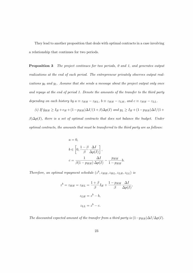
They lead to another proposition that deals with optimal contracts in a case involving

a relationship that continues for two periods.

Proposition 3 The project continues for two periods, 0 and 1, and generates output

realizations at the end of each period. The entrepreneur privately observes output real-

izations y0 and y1. Assume that she sends a message about the project output only once

and repays at the end of period 1. Denote the amounts of the transfer to the third party

depending on each history by a ≡ zHH − zHL, b ≡ zHH − zLH , and c ≡ zHH − zLL.

(i) If yHH ≥ IH +eH +(1−pHH)∆I/(1+β)∆p(I) and yL ≥ IH +(1−pHH)∆I/(1+

β)∆p(I), there is a set of optimal contracts that does not balance the budget. Under

optimal contracts, the amounts that must be transferred to the third party are as follows:

a = 0,

b ∈[0,

1 − β

β

∆I

∆p(I)

],

c =1

β(1 − pHH)∆I

∆p(I)− pHH

1 − pHHb.

Therefore, an optimal repayment schedule (zb, zHH , zHL, zLH , zLL) is

zb = zHH = zHL =1 + β

βIH +

1 − pHH

β

∆I

∆p(I),

zLH = zb − b,

zLL = zb − c.

The discounted expected amount of the transfer from a third party is (1−pHH)∆I/∆p(I).

23

The investor’s discounted expected payoff is (1 + β)IH and the entrepreneur’s is (1 +

β) {yHH − IH − (1 − pHH)∆I/(1 + β)∆p(I)}.

(ii) If either yHH < IH + eH + (1 − pHH)∆I/(1 + β)∆p(I) or yL < IH + (1 −

pHH)∆I/(1 + β)∆p(I), there are no efficient contracts.

The efficient and optimal contracts infinitely exist if and only if yHH and yL are

sufficiently large. The optimal contract specifies a repayment schedule such that a = 0,

i.e., zHH = zHL. This means that no money has to be transferred to a third party

to induce players to contribute significantly to the project in period 1 if the output

realization is large in period 0. Note that under such a contract, the investor will not

have any incentive to lend a large amount of money in period 1 as long as he knows

that y0 = yH has been realized at the end of period 0. The optimal contract provides

good incentive to the investor by hiding information on y0. Thus, an optimal contract

minimizes the discounted expected amount of money that must be transferred to a third

party; the minimum achieved value is (1 − pHH)∆I/∆p(I), which is the amount that,

at most, gives the investor a good incentive in period 0.

Since the discounted expected amount of the transfer is (1 + β)(1 − pHH)∆I/∆p(I)

when the entrepreneur sends a message in each period by the result of Proposition 2

(ii), the amount of transfer to a third party is reduced by not sending a message at

the end of period 0. Since players can reduce a reluctant transfer to a third party and

keep the investor’s expected discounted payoff identical to his discounted burden, the

24

entrepreneur’s expected discounted payoff increases. In addition, players can agree to

optimal contracts under smaller yHH and yL here than when the entrepreneur sends a

message in each period4.

4.2 The mutiperiod optimal financial contract without budget feasi-

bility constraint

The characteristics of venture capital contracts are similar to those of optimal contracts

presented in Proposition 3, except that in the former contracts a third party breaks

the budget by providing money for players but in the latter contracts he does so by

receiving money from players. Venture capitalists often invest in new firms by purchasing

convertible securities (Sahlman (1990)). If firms are profitable, venture capitalists often

recoup their investments through initial public offerings (Black and Gilson (1998) and

Gompers and Lerner (2004)). Venture capitalists contribute to projects not only by

financial assistance but also by management assistance, as do firms that contribute to

projects through their efforts. However, not all of their contributions can be specified in

a contract. Venture capitalists contribute to each project several times (stage financing)

but obtain a return only once: at the end of the relationship. If a venture firm is

profitable, the venture capitalist exercises a conversion option from debt to equity and

4When the entrepreneur sends a message and repays in each period, the efficient and optimal contacts

exist if and only if yHH ≥ eH + IH +(1−pHH)∆I/∆p(I) and yL ≥ IH +(1−pHH)∆I/∆p(I) as I sought

in Proposition 2.

25

obtains the right to take the firm’s surplus. If the venture firm is not profitable, the

venture capitalist requires the firm to pay back the debt or liquidate the firm.

Suppose that a venture capital contract requires that a firm pay zb as dividends when

he sends a good message and zb as liquidated values when he sends a bad message. The

firm is then indifferent to which messages he sends. Thus, firms always honestly report

the history of the output realizations. If the history is good, venture capitalists can

obtain capital gains through initial public offerings in addition to dividends. Therefore,

in this case, the amounts obtained by venture capitalists differ depending on the history,

but the amounts repaid by firms are constant. A third party or general outside investors

contribute funds to the players if the history is good, which is in contrast to the results

of Proposition 3, where the third party receives money from these players if the history

is bad. Here we assume zb ≤ zℓ for zℓ ∈ {zHH , zHL, zLH , zLL} and denote the amount

of the transfer from the third party depending on each history as a′ ≡ zLH − zLL,

b′ ≡ zHL − zLL, and c′ ≡ zHH − zLL.

If third party or general outside investors are too generous and buy a venture firm’s

share through initial public offerings for enough money to satisfy the individual ra-

tionality constraint for the venture capitalist, the venture firm, which minimizes the

repayment, never repays anything to the venture capitalist. In Proposition 4, we seek an

optimal venture contract when outside investors are rational and are not so generous to

minimize the amount they pay when buying the venture firm’s share through an initial

public offering.

26

Proposition 4 The project continues for two periods and generates output realization

at the end of each period. The entrepreneur privately observes output realizations y0 and

y1. She sends a message about the history of the output realizations and repays only once

at the end of the last period. We assume that markets for an initial public offering are

developed and a third party is willing to contribute a minimum fund that ensures high

contributions by both the entrepreneur and the investor.

(i) If yL ≥ IH−pHH∆I/(1+β)∆p(I), there is a set of optimal contracts that does not

balance the budget.5 Under optimal contracts, minimum values that must be transferred

from a third party are as follows:

a′ = 0,

b′ ∈[0,

1 − β

β

∆I

∆p(I)

],

c′ =1

βpHH

∆I

∆p(I)− 1 − pHH

pHHb′.

Therefore, an optimal repayment schedule (zb, zHH , zHL, zLH , zLL) is

zb = zLL = zLH =1 + β

βIH − pHH

β

∆I

∆p(I),

zHL =zb + b′,

zHH =zb + c′.

The discounted expected amount of the transfer from a third party is pHH∆I/∆p(I).

5In fact, there is a set of optimal contracts if and only if yHH ≥ eH + IH − pHH∆I/(1+ β)∆p(I) and

yL ≥ IH − pHH∆I/(1 + β)∆p(I). The condition on yHH is always true because of assumption (b).

27

The investor’s discounted expected payoff is (1 + β)IH and the entrepreneur’s is (1 +

β) {yHH − IH + pHH∆I/(1 + β)∆p(I)}.

(ii) If yL < IH − pHH∆I/(1 + β)∆p(I), there are no efficient contracts.

The optimal contract presented in Proposition 4 provides the sufficient conditions

under which such contracts exist, the minimum contribution by outside investors, and

the amounts the venture firm repays and the venture capitalist obtains. The optimal

contract specifies a repayment schedule such that a′ = 0, i.e., zLH = zLL. This means

that no money must be transferred by a third party if the output realization is small in

period 0. As in the case of Proposition 3, players minimize the amount of the transfer

from the third party by hiding information on the output realization in period 0. If this

type of outside investors and a market for initial public offering exist, an entrepreneur

can offer venture capital contracts to an investor. There is no requirement on yHH under

assumption (b) and the expected payoff for the entrepreneur is larger than that in the

case of Proposition 3; the entrepreneurs are more likely to offer efficient contracts to

investors than in the case of Proposition 3.

Even if players do not expect outside investors to pay sufficiently large amounts

for them or the markets for initial public offerings are underdeveloped or sluggish, the

entrepreneur can offer a contract such as that presented in Proposition 3 and pursue

efficient results. They are free to pay money to a third party, such as a charity.

28

5 conclusion

This paper seeks financial contracts that specify a repayment schedule that induces

both an investor and an entrepreneur to contribute to a project in every period and that

maximizes the entrepreneur’s expected payoff when the entrepreneur privately observes

project’s output realizations. To induce the entrepreneur to truthfully report output

realizations, repayments must be identical regardless of the history of the output re-

alizations. However, to induce both players to greatly contribute to the project, their

payoffs must reflect the history. Therefore, one type of optimal contract requires players

to directly transfer repayment from the entrepreneur to the investor if the history is good

and to pass some part of the money repaid by the entrepreneur to a third party and give

the rest to the investor if it is bad. Another type of optimal contract requires players to

directly transfer repayment from the entrepreneur to the investor if the history is bad

and to give money to the investor, money that the entrepreneur repays and that the

third party provides, if it is good.

When the project continues for two periods, contracts that require the entrepreneur

to deter reporting on output realizations and repaying the loan until the end of the last

period can reduce the amount of money that must be passed to or be provided by the

third party. When the entrepreneur hides information on the output realizations until

the end of the relationship, the contracts that give players good incentives in the first

period also can give them good incentives in the succeeding period. An example of the

29

budget-breaking financial contracts that expect a third party to pay money for players

depending on project’s performance is a venture capital contract, which expects general

investors to purchase venture firm’s shares if the project succeeds.

References

Bhattacharyya, Sugato and Francine Lafontaine (1995), “Double-Sided Moral Hazard

and the Nature of Share Contracts,” RAND Journal of Economics, Vol.26, No.4, pp.761-

781.

Black, Bernard S. and Ronald J. Gilson (1998),“Venture capital and the structure of

capital markets: banks versus stock markets ,” Journal of Financial Economics, Vol.47,

No.3, pp.243-277.

Bolton, Patrick and David S. Scharfstein (1990), “A Theory of Predation Based on

Agency Problems in Financial Contracting,” American Economic Review, Vol.80, No.1,

pp.93-106.

Diamond, Douglas W. (1984), “Financial Intermediation and Delegated Monitoring,”

Review of Economic Studies, Vol.51, No.3, pp.393-414.

Fuchs, William (2007), “Contracting with Repeated Moral Hazard and Private Evalua-

tions,” American Economic Review, Vol.97, No.4, pp.1432-1448.

Gale, Douglas and Martin Hellwig (1985), “Incentive-Compatible Debt Contracts: The

One-Period Problem,” Review of Economic Studies, Vol.52, No.4, pp.647-63.

30

Gompers, Paul A. and Lerner Josh (2006), The Venture Capital Cycle, 2nd Edition, The

MIT Press.

Holmstrom, Bengt (1982), “Moral Hazard in Teams,” Bell Journal of Economics, Vol.13,

No.2, pp.324-340

Kambe, Shinsuke (2006), “Subjective Evaluation In Agency Contracts,” Japanese Eco-

nomic Review,Vol. 57, No.1, pp.121-140.

MacLeod, W. Bentley (2003), “Optimal Contracting with Subjective Evaluation,” Amer-

ican Economic Review, Vol.93, No.1, pp.216-240.

Sahlman, William A. (1990), “The structure and governance of venture-capital organi-

zations,” Journal of Financial Economics, Vol.27, No.2, pp.473-521.

Townsend, Robert M. (1979), “Optimal contracts and competitive markets with costly

state verification,” Journal of Economic Theory, Vol.21, No.2, pp.265-293.

Appendix

Proof of Lemma 1

(i) Suppose ∆y ≥ ∆I/∆p(I) + ∆e/∆p(e). Then, there exists ∆rb such that ∆y −

∆e/∆p(e) ≥ ∆rb ≥ ∆I/∆p(I). When the budget balances , the schedule satisfies

constraints (7) and (8) simultaneously. Constraints (3) and (4) imply

yHH ≥ IH + eH + pHH(rbH − rℓ

H) + (1 − pHH)(rbL − rℓ

L). (9)

31

When the budget balances, this constraint is yHH ≥ IH + eH and always satisfied by

assumption (b).

(ii) Suppose ∆y < ∆I/∆p(I) + ∆e/∆p(e) and ∆rb satisfies (8). Then, there is no

∆rℓ which satisfies (7) when the budget balances. If ∆rℓ satisfies (7) and ∆rb satisfies

(8), i.e., rℓL ≤ rℓ

H − ∆I/∆p(I) and rbL ≥ rb

H − (∆y − ∆e/∆p(e)), we have

rbL − rℓ

L ≥{

rbH −

(∆y − ∆e

∆p(e)

)}−

{rℓH −

(∆I

∆p(I)

)}= (rb

H − rℓH) +

∆I

∆p(I)+

∆e

∆p(e)− ∆y.

To minimize the reluctant transfer to the third party, the repayment schedule satisfies

rbH = rℓ

H and rbL = rℓ

L+∆I/∆p(I)+∆e/∆p(e)−∆y. Considering this transfer, constraint

(9) can be written as yHH ≥ IH + eH + (1 − pHH) (∆I/∆p(I) + ∆e/∆p(e) − ∆y), i.e.,

yH ≥ IH + eH + (1 − pHH) (∆I/∆p(I) + ∆e/∆p(e)).

(iii) Suppose ∆y < ∆I/∆p(I) + ∆e/∆p(e). By the proof of Lemma 1(ii), if yH <

IH + eH + (1 − pHH) (∆I/∆p(I) + ∆e/∆p(e)) holds, players cannot make any efficient

contracts.

Proof of Proposition 1

(i) Suppose ∆y ≥ ∆I/∆p(I)+∆e/∆p(e). Then, efficient contracts are those that Lemma

1(i) specifies. The optimal contracts maximize the entrepreneur’s expected payoff; thus,

the individual rationality constraint for investor (3) binds, i.e., pHHrℓH + (1− pHH)rℓ

L =

IH . The pair (rℓH , rℓ

L) that satisfies this constraint and constraint (7) exists infinitely.

32

Therefore, the optimal contracts exist infinitely.

If we assume that constraint (7) binds, i.e., rℓH = rℓ

L + ∆I/∆p(I), constraint (3) is

pHH

(rℓL − ∆I/∆p(I)

)+ (1 − pHH)rℓ

L = IH . Then, we have rℓL = IH − pHH∆I/∆p(I),

and therefore, rℓH = IH +(1−pHH)∆I/∆p(I). Since the repayment balances the budget,

we have the results.

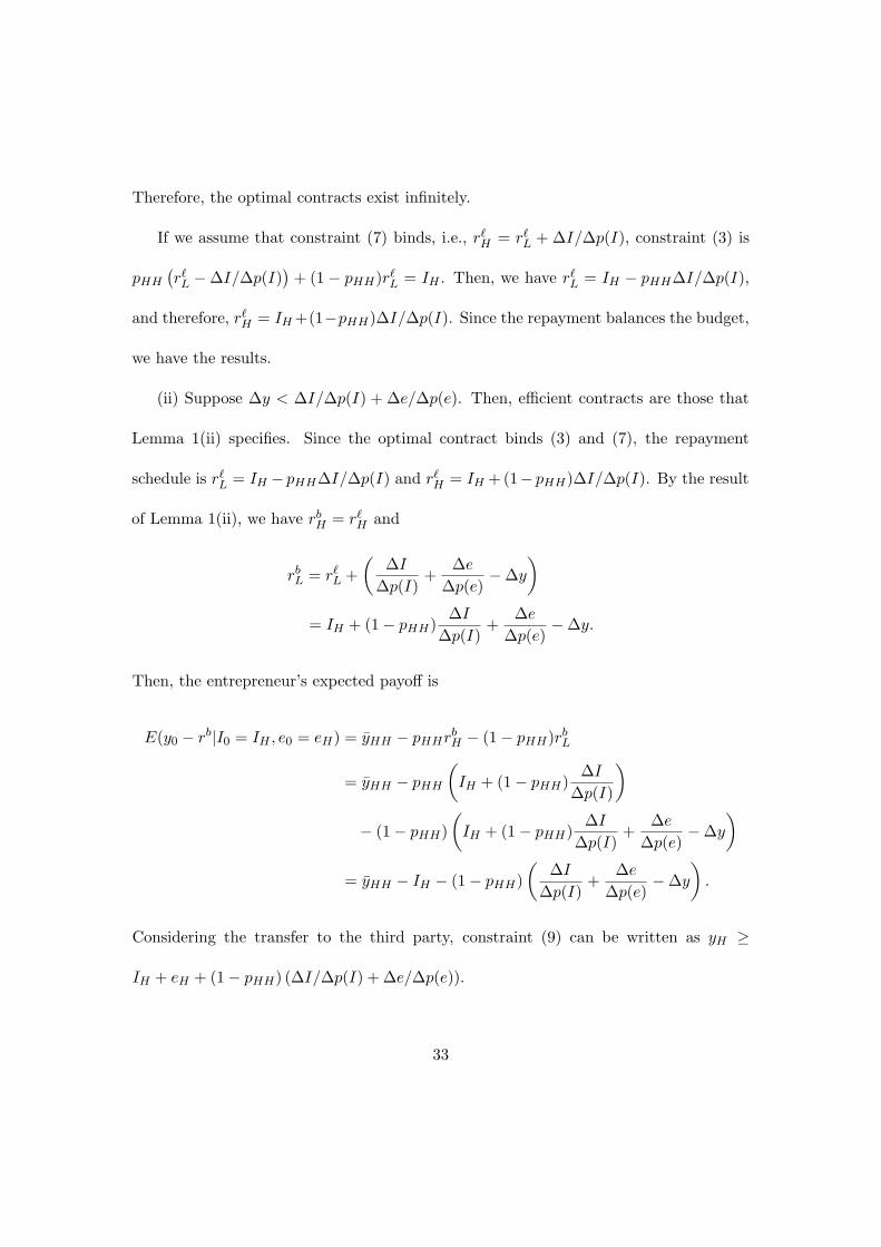
(ii) Suppose ∆y < ∆I/∆p(I) + ∆e/∆p(e). Then, efficient contracts are those that

Lemma 1(ii) specifies. Since the optimal contract binds (3) and (7), the repayment

schedule is rℓL = IH − pHH∆I/∆p(I) and rℓ

H = IH +(1− pHH)∆I/∆p(I). By the result

of Lemma 1(ii), we have rbH = rℓ

H and

rbL = rℓ

L +(

∆I

∆p(I)+

∆e

∆p(e)− ∆y

)= IH + (1 − pHH)

∆I

∆p(I)+

∆e

∆p(e)− ∆y.

Then, the entrepreneur’s expected payoff is

E(y0 − rb|I0 = IH , e0 = eH) = yHH − pHHrbH − (1 − pHH)rb

L

= yHH − pHH

(IH + (1 − pHH)

∆I

∆p(I)

)− (1 − pHH)

(IH + (1 − pHH)

∆I

∆p(I)+

∆e

∆p(e)− ∆y

)= yHH − IH − (1 − pHH)

(∆I

∆p(I)+

∆e

∆p(e)− ∆y

).

Considering the transfer to the third party, constraint (9) can be written as yH ≥

IH + eH + (1 − pHH) (∆I/∆p(I) + ∆e/∆p(e)).

33

Proof of Proposition 2

(i) To induce the entrepreneur to be honest about project output, players must set

∆rb = 0; in addition, to induce the investor to lend a large amount of money, they must

set ∆rℓ > 0. These constraints do not hold simultaneously if the repayment schedule

balances the budget.

(ii) There do not exist any efficient contracts which balance the budget. Then, the

optimal contract binds (3) and (7), and rℓH and rℓ

L are thus the as those in Proposition

1(ii). Since ∆rb = 0, constraint (8) can be rewritten by ∆y ≥ ∆e/∆p(e). ∆rb = 0 also

means that the transfer to the third party is ∆I/∆p(I) when the message is m0 = yL.

The entrepreneur always repays rℓH , i.e., rb

H = rbL = IH + (1 − pHH)∆I/∆p(I). Then,

yL ≥ IH+(1−pHH)∆I/∆p(I) must hold and the entrepreneur’s expected payoff is yHH−

IH − (1 − pHH)∆I/∆p(I). The individual rationality constraint for the entrepreneur

requires yHH ≥ IH + eH + (1 − pHH)∆I/∆p(I).

(iii) By the proof of Proposition 2(ii), if either yHH < IH +eH +(1−pHH)∆I/∆p(I)

or yL < IH + (1 − pHH)∆I/∆p(I), players cannot make any efficient contract.

Proof of Proposition 3

First, we seek optimal contracts which prevent the investor from deviating to lend a

small amount of money in either period 0 or period 1. Later, we show that this contract

is also the solution to the problem with the possibility to deviate twice by the investor.

34

Constraints (IC0) and (IC1) are rewritten as follows:

β{pHH(zHH − zLH) + (1 − pHH)(zHL − zLL)} ≥ ∆I

∆p(I), (IC0′)

β{pHH(zHH − zHL) + (1 − pHH)(zLH − zLL)} ≥ β∆I

∆p(I). (IC1′)

These constraints mean the discounted expected amount that must be transferred to the

third party. Using the definitions of a ≡ zHH −zHL, b ≡ zHH −zLH , and c ≡ zHH −zLL,

those constraints can be

pHH(a + b) + (1 − pHH)c ≥ ∆I

β∆p(I)+ a, (IC0′′)

pHH(a + b) + (1 − pHH)c ≥ ∆I

∆p(I)+ b. (IC1′′)

The individual rationality constraint for the investor is

β{(pHH)2zHH + pHH(1 − pHH)(zHH − a + zHH − b) + (1 − pHH)2(zHH − c)}

≥ (1 + β)IH .

This constraint can be

zHH ≥ 1 + β

βIH + (1 − pHH){pHH(a + b) + (1 − pHH)c}. (10)

The entrepreneur who wants to maximize her discounted expected payoffs minimizes

zHH subject to the constraints (IC0′′), (IC1′′), and (10); therefore, he minimizes the

expected amount of the transfer to the third party subject to these constraints.

Note that ∆I/β∆p(I) ≥ ∆I/∆p(I). To set a = 0 and b ∈ [0, (1 − β)∆I/β∆p(I)]

minimizes the amount of pHH(a + b) + (1 − pHH)c required by constraints (IC0′′) and

35

(IC1′′). Constraint (IC0′′), which prevents period 0 deviation, must bind, but constraint

(IC1′′), which prevents period 1 deviation, does not have to bind. c will be determined

by c = ∆I/β(1 − pHH)∆p(I) − pHHb/(1 − pHH).

The minimum amount of pHH(a + b) + (1 − pHH)c equals ∆I/β∆p(I); thus, the

optimal zHH is given as

zHH =1 + β

βIH + (1 − pHH) · ∆I

β∆p(I)=

1 + β

βIH +

1 − pHH

β

∆I

∆p(I).

Next, we show that the optimal contracts we have sought are optimal when we

add the possibility of deviating twice by the investor. Consider the constraint which

prevents the investor from deviating in period 1 given that he has deviated in period 0.

This constraint is

β {E(z|I0 = IL, I1 = IH) − E(z|I0 = I1 = IL)} ≥ β∆I. (IC3)

Like other constraints, it can be transformed as

pLH(zHH − zHL) + (1 − pLH)(zLH − zLL) ≥ ∆I

∆p(I), (IC3′)

i.e.,

pLHa + (1 − pLH)(c − b) ≥ ∆I

∆p(I). (IC3′′)

Constraint (IC1), which prevents period 1 deviation given that the investor has not

deviated in period 0, can be rewritten similarly as

pHHa + (1 − pHH)(c − b) ≥ ∆I

∆p(I). (IC1′′′)

36

Note that pHH > pLH and a = 0, and any pair (b,c) which satisfies (IC1′′′) satisfies

(IC3′′). It follows that any repayment schedule (zb, zHH , zHL, zLH , zLL) which satisfies

(IC1) satisfies (IC3). Combining (IC0) and (IC3), we have constraint (IC2). Therefore,

any repayment schedule (zb, zHH , zHL, zLH , zLL) which satisfies (IC0) and (IC1) satisfies

(IC2), and the optimal repayment schedule under constraints (IC0) and (IC1) is then

also optimal under constraints (IC0), (IC1), and (IC2).

Since the entrepreneur always repays zHH , the project’s property must satisfy (1 +

β)yL/β ≥ zHH , i.e., yL ≥ IH+(1−pHH)∆I/(1+β)∆p(I). The entrepreneur’s discounted

expected payoff is (1+β)(yHH−zHH) = (1+β) {yHH − IH − (1 − pHH)∆I/(1 + β)∆p(I)}

and therefore the individual rationality constraint for her implies yHH ≥ IH + eH +(1−

pHH)∆I/(1 + β)∆p(I).

Proof of Proposition 4

We will obtain the results in the same way as the proof of Proposition 3.

37