Grizzly Bear Cumulative Effects Assessment Model

Review For the Regional Carnivore Management Group

Grizzly Bear Cumulative Effects Assessment Model Review For the

Regional Carnivore Management Group

Prepared by G. Stenhouse1, Julie Dugas2, John Boulanger3, Dave Hobson2 and Helen Purves4

1 Gordon Stenhouse, Alberta Sustainable Resource Development, Fish and Wildlife

Division, and Foothills Model Forest, Box 6330, Hinton, Alberta, T7V 1X6. 2 Foothills Model Forest, Box 6330, Hinton, Alberta. T7V 1X6. 3 Integrated Ecological Research, 924 Innes Street, Nelson, British Columbia, V1L 5T2. 4 Jasper National Park, Box 10, Jasper, Alberta.

“The role of model testing is not to prove the truth of a model, which is impossible because models are never a perfect description of reality. Rather, testing should help identify the weakest aspects of models so they can be improved”. McCarty 2001.

Disclaimer The views, statements and conclusions expressed, and the recommendations made in this report are entirely those of the author(s) and should not be construed as statements or conclusions of, or as expressing the opinions of the Foothills Model Forest, or the partners or sponsors of the Foothills Model Forest. The exclusion of certain manufactured products does not necessarily imply disapproval, nor does the mention of other products necessarily imply endorsement by the Foothills Model Forest or any of its partners or sponsors.

ii

Executive Summary This report evaluates model runs from the grizzly bear Cumulative Effects Assessment (CEA) Model when compared with data gathered during the first three years of the Foothills Model Forest Grizzly Bear Research Program. The CEA model used habitat maps for the pre- and post-berry seasons and default assumptions on the effects of low and high intensity human use and linear features buffers used by Jasper National Park. The data gathered by the Foothills Model Forest Grizzly Bear Research Program included DNA mapping results and grizzly bear GPS telemetry locations. The model outputs evaluated are: • Habitat Effectiveness(HE) – The actual ability of an area to support grizzly bears

based on habitat values and the effects of human activities; • Security Areas – The identification of areas suitable to support a foraging adult

female grizzly bear. Individual model runs used the following assumptions: • Default parameters based on the CEA model assumptions and best available data; • Low human use assumption for all areas; • High human use assumption for all areas; • 50% buffer reduction for linear features; • 75% buffer reduction for linear features. Based on comparisons between model outputs and Foothills Model Forest data, Habitat Effectiveness and Security Area outputs were not significantly correlated to the distribution of bears from DNA data. These outputs were not correlated to level of use by GPS collared bears and were negatively correlated to the distribution of GPS collared bears. When compared with each other, the distribution of DNA bears and GPS bears were not correlated suggesting that the two methods were estimating different distributions. In this case, the DNA method was most likely the least biased as sampling effort was equal in each grid cell within a Bear Management Unit (BMU). CEA HE model outputs were also compared with Resource Selection Function (RSF) model probabilities. During the pre-berry season, at low HE values, RSF probabilities and HE outputs had a similar relationship. However, there was no relationship at higher HE values or in the post-berry season. Although model runs were not predictive of bear distribution, this failure does not necessarily mean that the model lacks validity. The model’s ability to predict grizzly bear use of BMUs may be enhanced through improvements to the base habitat map or by reassessing the assumptions used. Since these runs, an improved habitat map using an Integrated Decision Tree (IDT) process has been developed. Use of this product as a base habitat map may improve model effectiveness. Ongoing research into the effects of human access and intensity of human use on grizzly bear activity will be used to reassess the assumptions used in the model. The research may also identify other environmental or social factors that affect habitat use by grizzly bears and which may be incorporated into new approaches to understand relationships between grizzly bear habitat use and landscape conditions.

i

Table of Contents 1. Introduction..................................................................................................................... 1 2. Background..................................................................................................................... 1 3. Methods........................................................................................................................... 2

3.1. GIS layers used within the CEA model runs ........................................................... 3 3.2. Sources of Data:....................................................................................................... 3 3.3 Main Assumptions: ................................................................................................... 5 3.4. GIS Model Runs: ..................................................................................................... 6 3.5. Methods for comparison of DNA, radio telemetry outputs and CEA habitat effectiveness and security area........................................................................................ 8 3.6. Methods for comparison of CEA habitat effectiveness with RSF model outputs............................................................................................................................. 9 3.7. Methods for security area analysis......................................................................... 10

4. Results........................................................................................................................... 10 4.1. Habitat Effectiveness (HE) Analysis ..................................................................... 10

4.1.1. Comparison of HE between pre and post-berry seasons ................................ 10 4.1.1.1. Default Parameters................................................................................... 10 4.1.1.2. Human Use - Low.................................................................................... 11 4.1.1.3. Human Use - High ................................................................................... 11 4.1.1.4. Linear Feature Buffers – reduced by 50% ............................................... 12 4.1.1.5. Linear Feature Buffers – reduced by 75% ............................................... 13

4.1.2. Comparison of HE between default, low and high intensity runs .................. 13 4.1.3. Comparisons of HE between default, 50% and 75% linear features buffer reductions.................................................................................................................. 15 4.1.4. CEA Model HE Output – Distribution of GPS bears ..................................... 17 4.1.5. CEA Model HE Output – Comparison with RSF model outputs ................... 20

4.2. Security Area (SA) Analysis.................................................................................. 21 4.2.1. CEA Model SA Outputs – DNA Grizzly Bear Data....................................... 22 4.2.2. CEA Model SA Outputs – GPS Locations ..................................................... 22

5. Discussion and Conclusion ........................................................................................... 23 Appendix A....................................................................................................................... 25

ii

List of Figures Figure 1. EIA study area boundaries ............................................................................................................. 4 Figure 2. Grizzly Bear density within each BMU as determined through DNA hair snagging in 1999.

(Stenhouse and Munro 2000)................................................................................................................ 4 Figure 3. GPS Collar location data ................................................................................................................ 5 Figure 4. Relationship between habitat effectiveness and various measures of bear distribution and

use for individual BMU’s for the default values run of the CEA model (pre-berry season). Percentage of use (Ppoints) is the percentage of points (by individual bear) found in each BMU. GPS bears and DNA bears per 100km2 is the relative abundance of GPS and DNA bears in each BMU. Confidence intervals around regression lines are given to indicate the strength of apparent relationships. ........................................................................................................................ 18

Figure 5. Predicted relationship between RSF probabilities and CEA model habitat effectiveness from generalized additive model analysis for pre-berry runs. CEA model codes are: b5a-50% reduction of default buffer used, b7a-75% reduction of default buffer used, dpr-default values, hia-high intensity access, loa-low intensity access ............................................................................. 20

Figure 6. Predicted relationship between RSF probabilities and CEA model habitat effectiveness from generalized additive model analysis for post-berry model runs. CEA model codes are: b5b-50% reduction of default buffer used, b7b-75% reduction of default buffer used, dpo- default values, hib-high intensity access, lob-low intensity access..................................................... 21

Figure 7. The number of DNA bears identified per 100 km2 as a function of the percentage of security area in each BMU.................................................................................................................. 22

Figure 8. Relationship between relative use of BMU’s as indicated by percentage of points from GPS bears and the distribution of GPS bears in each BMU. .............................................................. 22

List of Tables Table 1. Habitat effectiveness for default model parameters in pre-berry and post-berry seasons.............. 10 Table 2. Habitat effectiveness for low human use intensity assumptions in pre-berry and post-berry

seasons. ............................................................................................................................................... 11 Table 3. Habitat effectiveness for high human use intensity in pre-berry and post-berry seasons .............. 12 Table 4. Habitat effectiveness for 50% linear features buffer reductions in pre-berry and post-berry

seasons. ............................................................................................................................................... 12 Table 5. Habitat effectiveness for 75% linear features buffer reduction in pre-berry and post-berry

seasons. ............................................................................................................................................... 13 Table 6. Habitat effectiveness for default, low human use and high human use intensity assumptions

for the pre-berry season. ..................................................................................................................... 14 Table 7. Habitat effectiveness for default, low human use and high human use intensity assumptions

for the post-berry season. .................................................................................................................... 15 Table 8. Habitat effectiveness for default, 50% and 75% buffer reduction assumptions for the pre-

berry season. ....................................................................................................................................... 16 Table 9. Habitat effectiveness for default, 50% and 75% buffer reduction assumptions for the post-

berry season. ....................................................................................................................................... 17 Table 10. Post-berry comparison of GPS statistics and cumulative effects runs by BMU........................... 19 Table 11. Pre-berry comparison of GPS/DNA statistics and cumulative effects runs by BMU................... 19 Table 12. Total area in each security/usability classification for each BMU ............................................... 21

iii

1. Introduction Land and resource managers have turned to cumulative effects assessment (CEA) models as tools to help with the assessment of how human activities within grizzly bear habitat may impact grizzly bear populations. Most of the elements of the current grizzly bear CEA models have been derived from standards put forward by the USDA Forest Service (1990). These CEA models have also been used in the Banff Park and Kananaskis area by Gibeau (1996) as well as within the context of environmental impact assessments for the proposed Cheviot Mine Project (BIOS 1996). In the Alberta portion of the Yellowhead Ecosystem there has been considerable interest in the ongoing and planned land use activities occurring along the eastern slopes within grizzly bear habitat. The overriding concern is that the cumulative impacts of these current and future activities may result in serious negative impacts for the grizzly bear population in this region. These concerns were brought to the forefront during the 1997 and 2000 EUB hearings into the proposed Cheviot open pit coal mine. The management response to these concerns was the preparation and endorsement of “A Strategic Framework for the Conservation of Grizzly Bears in the Alberta Yellowhead Ecosystem”, which now provides the management context for future resource management action. As part of the Strategic Framework, a Regional Carnivore Management Group (RCMG) was formed with representatives of both the federal and provincial governments as well as from the mining, forestry, and petroleum resource sectors. This group is tasked with reviewing the results of the Foothills Model Forest Grizzly Bear Research Program and using these findings to make recommendations to executive levels of government related to land use-planning activities in grizzly bear habitat in Alberta. 2. Background Over the past 5 years a number of open pit coal mine developments and expansions have been proposed along the foothills, within the Northern East Slopes Region, in recognized grizzly bear habitat. As part of the regulatory permitting requirements the companies involved have been required to conduct and submit environmental impact assessments related to the proposed activities. In the area south of Hinton, Alberta there have been three such undertakings over the past 5 years. These include: the proposed Cheviot Coal Mine Project (new mine), the Gregg River Mine (mine expansion), and the Luscar Coal Valley Mine (mine expansion) (Figure 1.). These three coal mining undertakings occur in relatively close proximity (all with 50 kms.) to each other yet each project was required to prepare an EIA document which included but was not limited to investigating the impact of the proposed activities on grizzly bears. Each of the projects defined an area surrounding their mine to which a cumulative effects assessment would be conducted. The size of the selected areas varied but all were approximately 3000 km2, which resulted in an overlap of assessment areas.

1

One task within the Foothills Model Forest Grizzly Bear Research Program was to conduct an evaluation of the current grizzly bear CEA models and to also provide land managers with an assessment of current landscape conditions relative to grizzly bears in the area. While it is recognized that CEA models were not constructed in a manner to undergo testing, it was felt that comparing the results of CEA model output with field data gathered from 1999-2001 within the research program would provide managers with a better understanding of the strengths and weaknesses of the current models. This level of understanding is important when making land management decisions involving the long-term conservation of grizzly bears. 3. Methods The CEA model evaluation was conducted in 3 phases: • Conduct model runs using default parameters from Purves and Doering (1998), high

and low human use intensity assumptions, and 50 and 75% linear feature buffer reductions.

• Compare model outputs with results of DNA mapping. • Compare model outputs with grizzly bear telemetry locations from 1999 to 2001.

The foundation of this report has been the GIS based Jasper National Park CEA application for grizzly bears developed by Purves and Doering (1998). This GIS based application is based on models described by Gibeau et al. 1996 and included three separate model elements: 1. Habitat effectiveness – which provides an analysis of existing habitat and human

activities to determine the actual ability to support grizzly bears; 2. Security areas – identification of areas suitable for individual foraging bouts for adult

female grizzlies based on ecological and human factors; 3. Linkage zones – identification of areas of potential movement for bears between

habitat areas based on landscape factors and human activities (Linkage zone analysis do not form part of this report, but are examined in more detail in relation to graph theory analysis currently underway.)

This report is not intended to provide a complete review of the CEA model and the reader is referred to both Gibeau et al. (1996) and USDA Forest Service (1990) for complete information on these models. An overview of current grizzly bear CEA models is presented in Appendix A, and the reader is referred to this section for further background information on these models. All model results presented in this report are from GIS model runs using the Purves and Doering (1998) application. There are four data sets that are used in the analysis presented in this report. The first data set is from the EIA documents provided by Luscar Limited from consultants retained to conduct the cumulative impact assessments on grizzly bears. This data set is made up of a number of components that are described further below. The second and third data sets are from the Foothills Model Forest Grizzly Bear Research Program. The second data set

2

represents the results of a DNA population census effort that was undertaken in 1999 in the research study area (Figure 2). The methodology and results of this census are provided in Stenhouse and Munro (1999 and 2000). The third data set is comprised of GPS radio collar data showing locations of grizzly bears for the period 1999-2001. For full details on these data the reader is referred to Stenhouse and Munro (1999 and 2000). The fourth data set used is from research conducted by Popplewell (2001) in which landscape metrics were calculated for the BMUs within the study area. 3.1. GIS layers used within the CEA model runs It should be noted that we utilized many different GIS layers to provide the best available approximation of human activities on the landscape, and grizzly bear habitat mapping that was available from the work done by BIOS (1996 and 2000). We recognize that these layers are not truly indicative of current landscape conditions and some habitats, access, and levels of human use may be different at the time of preparation of this report. In general terms the CEA application requires that data is available to allow: • the identification of Bear Management Units (BMU); • the documentation of various quality bear habitat for the pre berry (den emergence to

July 15) and post berry (July 15 – denning) seasons; • spatial representation of existing human access and settlements; and • the quantification of the amount of human activity associated with the human

features. Eight different spatial data layers are required to run the three Cumulative Effects Assessment (CEA) Models (Purves and Doering 1998). Four of these layers include the human use layers represented as lines, points, and polygons and the grizzly bear habitat layer. These four layers demanded the most attention in getting the best available seamless data set over the study area. 3.2. Sources of Data: The human use and habitat data were obtained from many different sources including: • 1997 Cheviot CEA data (obtained from John Kansas), • 1999 CEA data from Gregg River Mine, Cheviot Mine and the Coal Valley Mine

(obtained from Richard Ashton), • Jasper National Park (obtained from Helen Purves), • Weldwood of Canada (Hinton Division), • Weyerhaeuser Canada (Edson), • Sundance Forest Industries (Edson), • Alberta Environment (now Alberta Sustainable Resource Development).

3

Figure 1. EIA study area boundaries.

Figure 2. Grizzly Bear density within each BMU as determined through DNA hair snagging in 1999 (Stenhouse and Munro 2000).

4

Figure 3. GPS Collar location data. 3.3 Main Assumptions: Assumptions were made to deal with the various sources of data and the methods used to collect that data. These assumptions included: 1. The CEA model runs discussed in this paper were done by expressing the level of human use on an exponential scale as described in the table below.

Level of Use Definition 0 No use 1 1 to 10 events per month 2 11 to 100 events per month 3 101 to 1000 events per month 4 1001 to 10,000 events per month 5 10,001 to 100,000 events per month 6 100,001 to 1,000,000 events per month

The levels of human use defined for the environmental assessments (EA) of the three mines, were either LOW, HIGH or NONE. The CEA models require that this data be represented on an exponential scale. The assumption was made that LOW = 1, HIGH = 3 and NONE = 0. The CEA models use the scale of 2 as a cut-off between low and high human use, therefore setting high to a scale of 3 is sufficient for the purpose of these models (even if the actual human use is much higher).

5

2. The second assumption dealt with defining which data source was given precedence over another, based on extent and accuracy. As a general rule, the provincial data on access infrastructure was used as the basis for the human use layers. Within the provincial data, however, additional rules were made for features sharing the same spatial linework (an arc representing more than one feature): roads and railways overruled utility linework (pipeline and transmission lines), which in turn overruled seismic linework. Wherever there was overlap between data from Jasper National Park (JNP) and other data, JNP’s data took precedence as they maintain their data on a continuing basis and is assumed to be more accurate. 3. Weldwood forestry roads are mostly digitized and are updated on a yearly basis. The roads are classed differently and had to be re-classified to fit the feature codes used by the provincial data set. Class 1 = 2 lane gravel road. Class 2 = 2 lane gravel road. Class 3 & 4a = 1 lane gravel road. Class 4b = unimproved (temporary cutblock road). Class 5 = winter roads between cutblocks. 4. The CEA models require a grizzly bear habitat layer containing habitat values between 1.0 and 10.0. However, the habitat layers received from the mine EIAs were rated based on a Habitat Suitability Index (HSI). The HSI values between the mines (where overlap occurred) were slightly different for some polygons. The following strategy was used to deal with this issue. Where values were different between data sources, a high and low value was recorded and the mean value calculated. G.B.Stenhouse then classed these values into 10 categories to match the JNP habitat layer. 3.4. GIS Model Runs: The following procedures were used to create the human use linear features layer: 1. Use the provincial base data (Alberta) for features outside of Jasper as the basis of the

layer. 2. Supplement this data with roads/updates from forestry companies (Weldwood,

Weyerhaeuser and Sundance) where applicable. 3. Add Jasper National Park’s data to fill the area outside of the provincial landbase (as

it does not include the National Parks). 4. Compare with the mine EIA data and update as required. 5. Attach the known attribute data obtained from the Coal Branch CEAs. 6. Attach attribute data for the remainder of our features – either by known census data

or by expert opinion. Advantages: 1. Using the provincial base data as our main layer assured the best consistency

throughout the area outside Jasper National Park. We can also extend the boundary as far as the data will let us, which would be quite large.

2. Future updates would most likely be obtained from the same sources (government & forestry) – so integration should be relatively easy, as linework will match.

6

3. Same thing applies to Jasper data, except their updates may result in more accurate features. But that’s okay since, in comparison, their features are few and far between.

4. A prepared data set that is regularly maintained will provide future managers with the necessary tools to do other analysis (i.e. CEA).

Disadvantages: 1. Known attribute data will be relatively easy to assign, but unknown attribute data

remains a concern. 2. Updates or verification of these attributes is also a concern. Although further linework can be added through heads-up digitizing on recent orthophotos, it is best to stay with the best available data that is used by most major organizations. This ensures that the layers can be easily reproducible and avoids individual interpretation errors. For the first phase of the model evaluation, runs were made for both pre-berry and post-berry seasons. The default runs for both seasons placed the default buffers around the human constructed linear features (Purves and Doering 1998). These were 800 metres for features involving motorized activity and 400 metres for features involving non-motorized human activity. The default runs also used the best available data for intensity of human use within each Bear Management Unit (BMU). Following the default runs, two model runs were made in each season with 50 and 75% reductions in the default linear feature buffers and two runs were made in each season assuming all BMUs had either low use intensity (1-100 disturbances/month) or high use intensity (>100 disturbances/month). The results of each run placed each BMU into one of four categories based on level of habitat effectiveness (realized vs. potential habitat, expressed as a percentage). These categories are: • secure (>90% habitat effectiveness); • moderately threatened (>80% and ≤90% habitat effectiveness); • highly threatened (>70% and ≤80% habitat effectiveness); • severely impacted (≤70% habitat effectiveness). Following the runs, model outputs were compared with grizzly bear density estimates for each BMU based on DNA analysis of hair samples collected during 1999. DNA from hair collected in barbed wire snags placed throughout the study area was used to identify individual grizzly bears and generate density estimates for each BMU. Finally, model outputs were compared with grizzly bear telemetry points collected between 1999 and 2001. Due to the large number of telemetry points collected during this period, a random sample of one point per day per bear for each year for a total of 4151 telemetry points were used in this analysis.

7

The security area model identifies areas that are suitable for individual foraging bouts for adult female grizzly bears. Size of the area and amount of human activity affect the outputs from this model. Areas <9 km2 are not considered secure. High intensity human use features are buffered. Areas within the buffer are not considered secure. Finally, areas > 2300m altitude and areas consisting of non-vegetated rock, snow or ice are not considered useable. Model outputs are in two formats. Total areas (km2) are calculated for secure, non-secure (size), non-secure (human), useable and unusable habitats. Percentages of total area are calculated for secure, non-secure (size), non-secure (human), useable, unusable and secure/useable habitat. For the model evaluation, we used the total area (km2) of secure/usable habitat in each BMU using the default assumptions and best available data. These totals were compared with the DNA grizzly bear density estimates, fragmentation as determined by landscape metrics, and telemetry location points from radio-collared grizzly bears for each BMU. The McLeod and Lovett BMUs were not included in the analysis due to a lack of complete coverage in each unit. 3.5. Methods for comparison of DNA, radio telemetry outputs and CEA habitat effectiveness and security area A previous analysis compared cumulative effects predictions with pooled GPS locations of bears, and the frequency of bears identified in bear management units (BMUs) to determine if cumulative effect models could predict bear use of habitats. One of the noted limitations of the comparison of pooled GPS points with predicted densities/use of habitat/BMUs by bears is that the amount of use in any BMU will be somewhat determined by the overall distribution of GPS bears. This analysis explores a potential way to partially mitigate this issue by using individual bears as the sampling unit rather than pooled locations. The following procedure was used.

a) The percentage of points occurring in each BMU was tallied for each GPS bear for each season and year of the analysis.

b) For each BMU the corresponding percentage of points from each bear that had at least one point in the BMU was averaged. If a bear used a BMU for more than one year then the percentage of points for this bear was first averaged to give an overall average for the given bear, which was then averaged with other bears.

c) So for each BMU, an average proportion of points for each bear that could have potentially used the BMU were estimated (Ppoints). This gave an index of habitat use for each BMU. In addition, the number of GPS bears utilizing each BMU was tallied (NGPS) as an index of overall distribution of bears assuming that the distribution of GPS bears was indicative of the overall distribution of bears in the Foothills study area. This assumption was tested by comparing the distribution of unique bears identified in each BMU using DNA (NDNA) methods with the distribution of GPS bears.

d) One added issue was that BMUs differed in area, which influenced the number of GPS, and DNA bears found in each BMU. Because this factor could potentially

8

complicate comparisons, each count was standardized by the area of corresponding BMU (DGPS and DDNA). Note that these standardized counts are not a density estimate since counts constitute a measure relative abundance rather than a population estimate.

The main potential advantage of the Ppoints index over indices that pool locations (previous analysis and Npoints) is that it should be not as affected by the distribution of GPS bears on the study area. It will also more directly reflect the actual number of independent units (i.e. bears) used to get estimates, rather than using pooled points as the sample unit which is more influenced by pseudoreplication, autocorrelation, and other statistical issues (Otis and White 1999). Correlation analysis (Zar 1996) was used to determine if habitat effectiveness was associated with the number of GPS bears (NGPS and DGPS), mean percentage of points per bear (Ppoints), or the distribution of DNA bears (NDNA and DDNA) for each combination of BMU, season, and cumulative effects model run. Plots of the data were also used to determine if weak associations existed that were not detected by correlations analyses. 3.6. Methods for comparison of CEA habitat effectiveness with RSF model outputs Resource selection function habitat analysis was conducted using GPS points for grizzly bears from 1999-2001 (Neilson 2002). The RSF model produced probabilities of occurrence for 50m cells for the Foothills study area. These were randomly sampled to produce 1000 cells with paired RSF probabilities and habitat effectiveness values. These paired values were then compared to determine the correspondence between RSF probabilities and habitat effectiveness values. This approach was superior to BMU-based comparison given the large degree of variance in RSF probabilities within any given BMU. The main objective of comparisons was to determine if there was an underlying relationship between RSF and CEA model outputs. The second objective was to determine if there was a difference in the underlying relationship between different model runs of the CEA model. This relationship could potentially take many forms from a simple linear relationship to a non-linear relationship. For example, RSF probabilities may correspond to CEA model outputs for lower RSF probabilities, and then not correspond for higher RSF probabilities. Generalized additive models were used for the relationship between habitat predictor variables and the response presence/absence data (Bio et al. 1998). Generalized additive models attempt to fit a linear term and a cubic spline term in which the data is smoothed to the best fitting non-linear curve (Hastie and Tibshirani 1990). The significance of the linear and spline terms was then evaluated to determine if non-linear trends existed. A generalized cross validation procedure was used to select values for smoothing parameters. If significant non-linear trends existed, then the relationship between RSF probabilities and CEA habitat effectiveness was plotted to determine the shape and biological significance of the relationship. SAS PROC GAM was used for this analysis (SAS Institute 2000).

9

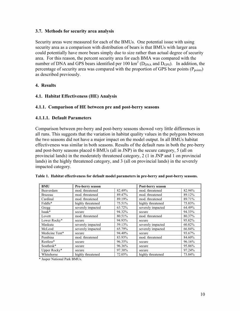
3.7. Methods for security area analysis Security areas were measured for each of the BMUs. One potential issue with using security area as a comparison with distribution of bears is that BMUs with larger area could potentially have more bears simply due to size rather than actual degree of security area. For this reason, the percent security area for each BMA was compared with the number of DNA and GPS bears identified per 100 km2 (DDNA and DGPS). In addition, the percentage of security area was compared with the proportion of GPS bear points (Ppoints) as described previously. 4. Results 4.1. Habitat Effectiveness (HE) Analysis 4.1.1. Comparison of HE between pre and post-berry seasons 4.1.1.1. Default Parameters Comparison between pre-berry and post-berry seasons showed very little differences in all runs. This suggests that the variation in habitat quality values in the polygons between the two seasons did not have a major impact on the model output. In all BMUs habitat effectiveness was similar in both seasons. Results of the default runs in both the pre-berry and post-berry seasons placed 6 BMUs (all in JNP) in the secure category, 5 (all on provincial lands) in the moderately threatened category, 2 (1 in JNP and 1 on provincial lands) in the highly threatened category, and 3 (all on provincial lands) in the severely impacted category. Table 1. Habitat effectiveness for default model parameters in pre-berry and post-berry seasons.

BMU Pre-berry season Post-berry season Beaverdam mod. threatened 82.49% mod. threatened 82.94% Brazeau mod. threatened 89.47% mod. threatened 89.12% Cardinal mod. threatened 89.19% mod. threatened 89.71% Fiddle* highly threatened 75.51% highly threatened 75.83% Gregg severely impacted 63.72% severely impacted 64.49% Isaak* secure 94.32% secure 94.33% Lovett mod. threatened 80.51% mod. threatened 80.37% Lower Rocky* secure 94.93% secure 95.82% Maskuta severely impacted 59.13% severely impacted 60.82% McLeod severely impacted 65.79% severely impacted 66.84% Medicine Tent* secure 94.40% secure 93.67% Pembina mod. threatened 83.93% mod. threatened 84.60% Restless* secure 96.35% secure 96.16% Southesk* secure 96.36% secure 95.86% Upper Rocky* secure 97.38% secure 97.24% Whitehorse highly threatened 72.05% highly threatened 73.84%

* Jasper National Park BMUs.

10

4.1.1.2. Human Use - Low Results of the low human use model runs (all human use features were rated as low use) also showed similarities between pre- and post-berry season output. Nine BMUs (6 in JNP and 3 on provincial lands) were secure in the pre-berry season compared with 10 secure BMUs (6 in JNP and 4 on provincial lands) in the post-berry season. Seven BMUs (6 on provincial lands and 1 in JNP) were moderately threatened in the pre-berry season compared with 6 moderately threatened BMUs (5 on provincial lands and 1 in JNP) in the post-berry season. Only the Pembina BMU had different habitat effectiveness rating between the pre- and post-berry season. None of the BMUs were either highly threatened or severely impacted in either season. Table 2. Habitat effectiveness for low human use intensity assumptions in pre-berry and post-berry seasons.

BMU Pre-berry season Post-berry season Beaverdam secure 90.80% secure 91.09% Brazeau secure 94.58% secure 94.32% Cardinal secure 95.05% secure 95.30% Fiddle* mod. threatened 87.27% mod. threatened 87.51% Gregg mod. threatened 81.21% mod. threatened 81.56% Isaak* secure 95.03% secure 94.95% Lovett mod. threatened 89.76% mod. threatened 89.81% Lower Rocky* secure 97.29% secure 97.67% Maskuta mod. threatened 80.67% mod. threatened 81.60% McLeod mod. threatened 82.83% mod. threatened 83.40% Medicine Tent* secure 94.40% secure 93.67% Pembina mod. threatened 89.85% secure 90.51% Restless* secure 96.35% secure 96.16% Southesk* secure 96.36% secure 95.86% Upper Rocky* secure 97.63% secure 97.51% Whitehorse mod. threatened 84.93% mod. threatened 85.93%

* Jasper National Park BMUs. 4.1.1.3. Human Use - High Results of high human use runs (all human use features were rated as high use) were similar between seasons. Two BMUs (both in JNP) were secure in both the pre- and post-berry seasons. Seven (4 in JNP and 3 on provincial lands) were moderately threatened in both seasons. Three (2 on provincial lands and 1 in JNP) were highly threatened in the pre-berry season compared with 4 (3 on provincial lands and 1 in JNP) in the post-berry season. Four (all on provincial lands) were severely impacted in the pre-berry season compared with 3 (all on provincial lands) in the post-berry season.

11

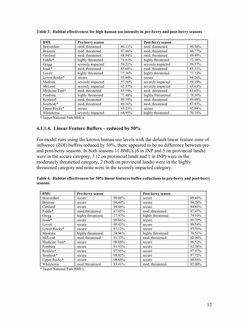
Table 3. Habitat effectiveness for high human use intensity in pre-berry and post-berry seasons

BMU Pre-berry season Post-berry season Beaverdam mod. threatened 80.11% mod. threatened 80.56% Brazeau mod. threatened 87.46% mod. threatened 86.77% Cardinal mod. threatened 88.94% mod. threatened 89.49% Fiddle* highly threatened 71.51% highly threatened 72.10% Gregg severely impacted 59.21% severely impacted 59.57% Isaak* mod. threatened 85.68% mod. threatened 85.51% Lovett highly threatened 77.36% highly threatened 77.15% Lower Rocky* secure 93.44% secure 94.26% Maskuta severely impacted 57.56% severely impacted 59.19% McLeod severely impacted 62.57% severely impacted 63.63% Medicine Tent* mod. threatened 83.59% mod. threatened 81.65% Pembina highly threatened 77.48% highly Threatened 78.50% Restless* mod. threatened 89.59% mod. threatened 89.09% Southesk* mod. threatened 89.26% mod. threatened 87.87% Upper Rocky* secure 93.25% secure 92.84% Whitehorse severely impacted 68.95% highly threatened 70.74%

* Jasper National Park BMUs 4.1.1.4. Linear Feature Buffers – reduced by 50% For model runs using the known human use levels with the default linear feature zone of influence (ZOI) buffers reduced by 50%, there appeared to be no difference between pre- and post-berry seasons. In both seasons 11 BMUs (6 in JNP and 5 on provincial lands) were in the secure category, 3 (2 on provincial lands and 1 in JNP) were in the moderately threatened category, 2 (both on provincial lands) were in the highly threatened category and none were in the severely impacted category. Table 4. Habitat effectiveness for 50% linear features buffer reductions in pre-berry and post-berry seasons.

BMU Pre-berry season Post-berry season Beaverdam secure 90.08% secure 90.49% Brazeau secure 94.44% secure 94.28% Cardinal secure 94.46% secure 94.83% Fiddle* mod. threatened 87.05% mod. threatened 87.47% Gregg highly threatened 77.97% highly threatened 79.10% Isaak* secure 96.66% secure 96.70% Lovett secure 90.43% secure 90.54% Lower Rocky* secure 97.12% secure 97.76% Maskuta highly threatened 74.96% highly threatened 76.51% McLeod mod. threatened 81.37% mod. threatened 82.04% Medicine Tent* secure 96.88% secure 96.52% Pembina secure 91.93% secure 92.38% Restless* secure 97.95% secure 97.97% Southesk* secure 98.02% secure 97.72% Upper Rocky* secure 98.60% secure 98.56% Whitehorse mod. threatened 83.41% mod. threatened 85.00%

* Jasper National Park BMUs.

12

4.1.1.5. Linear Feature Buffers – reduced by 75% For model runs using the known human use levels with the default linear feature ZOI buffers reduced by 75%, there appeared to be little difference between pre- and post-berry seasons. Only 1 BMU had a different ranking between the two seasons relative to habitat effectiveness. Thirteen BMUs (7 in JNP and 6 on provincial lands) were in the secure category in the pre-berry season compared with 14 (7 in JNP and 7 on provincial lands) in the post-berry season. Three (all on provincial lands) were in the moderately threatened category in the pre-berry season compared with 2 (both on provincial lands) in the post-berry season. In both seasons none were in the highly threatened and severely impacted categories. Table 5. Habitat effectiveness for 75% linear features buffer reduction in pre-berry and post-berry seasons.

BMU Pre-berry season Post-berry season Beaverdam secure 94.61% Secure 94.85% Brazeau secure 97.17% Secure 97.14% Cardinal secure 97.16% Secure 97.40% Fiddle* secure 93.06% Secure 93.44% Gregg mod. threatened 87.67% mod. Threatened 88.49% Isaak* secure 97.93% Secure 97.96% Lovett secure 94.91% Secure 95.10% Lower Rocky* secure 98.36% Secure 98.78% Maskuta mod. threatened 86.03% mod. Threatened 87.10% McLeod secure 89.90% mod. Threatened 90.25% Medicine Tent* secure 98.16% Secure 97.98% Pembina secure 95.87% Secure 96.12% Restless* secure 98.87% Secure 98.93% Southesk* secure 98.87% Secure 98.70% Upper Rocky* secure 99.23% Secure 99.22% Whitehorse secure 90.14% Secure 91.29%

* Jasper National Park BMUs. Comparisons between pre- and post-berry seasons in all runs suggest that the habitat effectiveness model was not sensitive to the habitat variations between seasons. Those BMUs that did show a change in habitat effectiveness categories between seasons were not significantly different in percentage of realised vs. potential habitat. They simply fell on either side of the arbitrary boundary between categories. 4.1.2. Comparison of HE between default, low and high intensity runs Comparisons were made between the pre-berry season default, low human use intensity and high human use intensity runs. The default habitat effectiveness (HE) outputs were similar to high intensity HE outputs in 8 BMUs (7 on provincial lands and 1 in JNP). The default HE outputs was similar to low intensity HE outputs in 6 BMUs (5 in JNP and 1 on provincial lands). Default HE outputs for 2 BMUs (1 on provincial lands and 1 in JNP) showed no greater similarity to either high or low intensity HE outputs.

13

Pre-berry habitat effectiveness outputs for the default run placed 6 BMUs (all in JNP) in the secure category compared with 9 (6 in JNP and 3 on provincial lands) in the low intensity run and 2 (both in JNP) in the high intensity run. Five BMUs (all on provincial lands) in the default run were placed in the moderately threatened category compared with 7 (all on provincial lands) in both low and high intensity runs. Two BMUs (all on provincial lands) in the default run were highly threatened compared with 3 (all on provincial lands) in the high intensity run and 0 in the low intensity run. Three BMUs (all on provincial lands) in the default run were severely impacted compared with 4 (all on provincial lands) in the high intensity run and 0 in the low intensity run. Table 6. Habitat effectiveness for default, low human use and high human use intensity assumptions for the pre-berry season.

BMU Default run Low intensity run High intensity run Beaverdam mod. threatened 82.49% secure 90.80% mod. threatened 80.11% Brazeau mod. threatened 89.47% secure 94.58% mod. threatened 87.46% Cardinal mod. threatened 89.19% secure 95.05% mod. threatened 88.94% Fiddle* highly threatened 75.51% mod. threatened 87.27% highly threatened 71.51% Gregg severely impacted 63.72% mod. threatened 81.21% severely impacted 59.21% Isaak* secure 94.32% secure 95.03% mod. threatened 85.68% Lovett mod. threatened 80.51% mod. threatened 89.76% highly threatened 77.36% Lower Rocky* secure 94.93% secure 97.29% secure 93.44% Maskuta severely impacted 59.13% mod. threatened 80.67% severely impacted 57.56% McLeod severely impacted 65.79% mod. threatened 82.83% severely impacted 62.57% Medicine Tent* secure 94.40% secure 94.40% mod. threatened 83.59% Pembina mod. threatened 83.93% mod. threatened 89.85% highly threatened 77.48% Restless* secure 96.35% secure 96.35% mod. threatened 89.59% Southesk* secure 96.36% secure 96.36% mod. threatened 89.26% Upper Rocky* secure 97.38% secure 97.63% secure 93.25% Whitehorse highly threatened 72.05% mod. threatened 84.93% severely impacted 68.95%

* Jasper National Park BMUs. Comparisons between HE outputs in default, high intensity and low intensity runs during the post-berry season were similar to the pre-berry season. HE outputs in 9 BMUs (8 on provincial lands and 1 in JNP) in the default run were similar to HE outputs in BMUs in the high intensity run. HE outputs in 5 BMUs (all in JNP) in the default run were similar to HE outputs in BMUs in the low intensity run. HE outputs in 2 BMUs (1 on provincial lands and 1 in JNP) in the default run showed no greater similarity to either high or low intensity HE outputs. Post-berry habitat effectiveness outputs for the default run placed 6 BMUs (all in JNP) in the secure category compared with 10 (6 in JNP and 4 on provincial lands) in the low intensity run and 2 (both in JNP) in the high intensity run. In the default run, 5 BMUs (all on provincial lands) were considered moderately threatened compared with 6 (all on provincial lands) in the low intensity run and 7 (3 on provincial lands and 4 in JNP) in the high intensity run. There were 2 and 4 BMUs (all on provincial lands) in the highly threatened category in the default and high intensity runs respectively. Three BMUs were considered severely impacted in both default and high intensity runs. There were no BMUs listed as highly threatened or severely impacted in the low intensity run.

14

Table 7. Habitat effectiveness for default, low human use and high human use intensity assumptions for the post-berry season.

BMU Default run Low intensity run High intensity run Beaverdam mod. threatened 82.94% secure 91.09% mod. threatened 80.56% Brazeau mod. threatened 89.12% secure 94.32% mod. threatened 86.77% Cardinal mod. threatened 89.71% secure 95.30% mod. threatened 89.49% Fiddle* highly threatened 75.83% mod. threatened 87.51% highly threatened 72.10% Gregg severely impacted 64.49% mod. threatened 81.56% severely impacted 59.57% Isaak* secure 94.33% secure 94.95% mod. threatened 85.51% Lovett mod. threatened 80.37% mod. threatened 89.81% highly threatened 77.15% Lower Rocky* secure 95.82% secure 97.67% secure 94.26% Maskuta severely impacted 60.82% mod. threatened 81.60% severely impacted 59.19% McLeod severely impacted 66.84% mod. threatened 83.40% severely impacted 63.63% Medicine Tent* secure 93.67% secure 93.67% mod. threatened 81.65% Pembina mod. threatened 84.60% secure 90.51% highly threatened 78.50% Restless* secure 96.16% secure 96.16% mod. threatened 89.09% Southesk* secure 95.86% secure 95.86% mod. threatened 87.87% Upper Rocky* secure 97.24% secure 97.51% secure 92.84% Whitehorse highly threatened 73.84% mod. threatened 85.93% highly threatened 70.74%

* Jasper National Park BMUs. Comparisons between intensity of human use assumptions in each season suggest that the habitat effectiveness model is highly sensitive to changes in human use intensity. Changes in human use intensity from low to high resulted in a decrease in habitat effectiveness. The BMUs on provincial land tended to have default outputs closer to high intensity outputs then to low intensity outputs. The opposite was seen for BMUs in Jasper National Park where default outputs tended to be closer to low intensity outputs then to high intensity outputs. 4.1.3. Comparisons of HE between default, 50% and 75% linear features buffer reductions Comparisons were made between default, 50%, and 75% linear feature buffer reductions for the pre-berry season. With the 75% buffer reduction run, 13 BMUs (7 on provincial lands and 6 in JNP) were placed in the secure category compared with 11 (5 on provincial lands and 6 in JNP) for the 50% buffer reduction run and 6 (all in JNP) in the default run. Three BMUs (all on provincial lands) were considered moderately threatened in the 75% buffer reduction run compared with 3 and 5 BMUs (all on provincial lands) in the 50% buffer reduction and default runs respectively. The 75% buffer reduction run had no BMUs listed as highly threatened or severely impacted. The 50% buffer reduction run had 2 BMUs (both on provincial lands) considered highly threatened and 0 considered severely impacted. The default run had 2 BMUs (all on provincial lands) listed as highly threatened and 3 (all on provincial lands) as severely impacted. As buffer size assumptions were reduced from 800m (default) to 400m (50% reduction) to 200m (75% reduction) for linear features with motorized activity and 400m (default) to 200m (50% reduction) to 100m (75% reduction) for linear features with non-motorized human activity, all BMUs increased in habitat effectiveness. Number of BMUs considered secure moved from 6 to 11 to 13 respectively. Number of BMUs considered

15

moderately threatened decreased from 5 to 3 to 2 respectively. Number of BMUs considered highly threatened decreased from 2 to 2 to 0 respectively. Number of BMUs considered severely impacted decreased from 3 to 0 to 0 respectively. Table 8. Habitat effectiveness for default, 50% and 75% buffer reduction assumptions for the pre-berry season.

BMU Default run 50% buffer reduction 75% buffer reduction Beaverdam mod. threatened 82.49% secure 90.08% secure 94.61% Brazeau mod. threatened 89.47% secure 94.44% secure 97.17% Cardinal mod. threatened 89.19% secure 94.46% secure 97.16% Fiddle* highly threatened 75.51% mod. threatened 87.05% secure 93.06% Gregg severely impacted 63.72% highly threatened 77.97% mod. threatened 87.67% Isaak* secure 94.32% secure 96.66% secure 97.93% Lovett mod. threatened 80.51% secure 90.43% secure 94.91% Lower Rocky* secure 94.93% secure 97.12% secure 98.36% Maskuta severely impacted 59.13% highly threatened 74.96% mod. threatened 86.03% McLeod severely impacted 65.79% mod. threatened 81.37% secure 89.90% Medicine Tent* secure 94.40% secure 96.88% secure 98.16% Pembina mod. threatened 83.93% secure 91.93% secure 95.87% Restless* secure 96.35% secure 97.95% secure 98.87% Southesk* secure 96.36% secure 98.02% secure 98.87% Upper Rocky* secure 97.38% secure 98.60% secure 99.23% Whitehorse highly threatened 72.05% mod. threatened 83.41% secure 90.14%

* Jasper National Park BMUs. Comparisons were made between default, 50%, and 75% linear feature buffer reductions for the post-berry season. Results were similar to pre-berry season comparisons with the 75% buffer reduction run. 14 BMUs (7 on provincial lands and 7 in JNP) were placed in the secure category compared with 11 (5 on provincial lands and 6 in JNP) for the 50% buffer reduction run and 6 (all in JNP) in the default run. Two BMUs (both on provincial lands) were considered moderately threatened in the 75% buffer reduction run compared with 3 and 5 BMUs (all on provincial lands) in the 50% buffer reduction and default runs respectively. The 75% buffer reduction run had no BMUs listed as highly threatened or severely impacted. The 50% buffer reduction run had 2 BMUs (both on provincial lands) considered highly threatened and 0 considered severely impacted. The default run had 2 BMUs (all on provincial lands) listed as highly threatened and 3 (all on provincial lands) as severely impacted. As buffer size assumptions were reduced from 800m (default) to 400m (50% reduction) to 200m (75% reduction) for linear features with motorized activity and 400m (default) to 200m (50% reduction) to 100m (75% reduction) for linear features with non-motorized human activity, all BMUs increased in habitat effectiveness. Number of BMUs considered secure was reduced from 14 to 11 to 6 respectively. Number of BMUs considered moderately threatened increased from 2 to 3 to 5 respectively. Number of BMUs considered highly threatened increased from 0 to 2 to 2 respectively. Number of BMUs considered severely impacted increased from 0 to 0 to 3 respectively.

16

Table 9. Habitat effectiveness for default, 50% and 75% buffer reduction assumptions for the post-berry season.

BMU Default run 50% buffer reduction 75% buffer reduction Beaverdam mod. threatened 82.94% secure 90.49% secure 94.85% Brazeau mod. threatened 89.12% secure 94.28% secure 97.14% Cardinal mod. threatened 89.71% secure 94.83% secure 97.40% Fiddle* highly threatened 75.83% mod. threatened 87.47% secure 93.44% Gregg severely impacted 64.49% highly threatened 79.10% mod. threatened 88.49% Isaak* secure 94.33% secure 96.70% secure 97.96% Lovett mod. threatened 80.37% secure 90.54% secure 95.10% Lower Rocky* secure 95.82% secure 97.76% secure 98.78% Maskuta severely impacted 60.82% highly threatened 76.51% mod. threatened 87.10% McLeod severely impacted 66.84% mod. threatened 82.04% mod. threatened 90.25% Medicine Tent* secure 93.67% secure 96.52% secure 97.98% Pembina mod. threatened 84.60% secure 92.38% secure 96.12% Restless* secure 96.16% secure 97.97% secure 98.93% Southesk* secure 95.86% secure 97.72% secure 98.70% Upper Rocky* secure 97.24% secure 98.56% secure 99.22% Whitehorse highly threatened 73.84% mod. threatened 85.00% secure 91.29%

* Jasper National Park BMUs. Comparisons between default and buffer reduction assumptions suggest that the habitat effectiveness model is sensitive to changes in linear features buffer size. A decrease in assumed buffer size resulted in an increase in habitat effectiveness. This effect was seen in BMUs on provincial lands where there are a large number of human-constructed linear features. Except for the Fiddle BMU, changes in buffer size assumptions did not result in a change in habitat effectiveness categories in the Jasper National Park BMUs. This is likely due to the low number of human-constructed linear features in Jasper. 4.1.4. CEA Model HE Output – Distribution of GPS bears Habitat effectiveness was not significantly correlated (at α=0.1) with the mean percentage of bear points per BMU (Ppoints) for any of the cumulative effects runs, or seasons considered. However, habitat effectiveness was negatively correlated with the number of GPS bears per 100 km2 in each BMU (DGPS) for most runs of the cumulative effects models. Habitat effectiveness was not significantly correlated with the number of DNA bears identified in each BMU per 100 km2, however, inspection of plots suggested a slight positive association. As illustrated in Figure 1, GPS bear abundance seemed to decrease at higher levels of habitat effectiveness whereas DNA bear abundance increased slightly. Tables 10 and 11 give a complete listing of results by BMU. The distribution of bears as estimated by GPS bears (NGPS) and distribution of DNA bears (NDNA) by BMU was not significantly correlated suggesting that GPS and DNA bears are estimating different distributions of bears on the study area. Of the two metrics, the DNA distribution is most likely to be unbiased since equal sampling effort was given to each of the BMU’s. Given this assumption, a slight positive association between habitat effectiveness and bear distribution is evident in Figure 4.

17

Perc

enta

ge u

se o

f BM

U

0.0

0.2

0.4

0.6

0.8

1.0

Habitat effectiveness

50 60 70 80 90 100

GPS

bea

rs/1

00km

2

0

1

2

3

4

Habitat effectiveness

50 60 70 80 90 100

DNA

bea

rs/1

00 k

m2

0

1

2

3

4

Habitat effectiveness

50 60 70 80 90 100

Figure 4. Relationship between habitat effectiveness and various measures of bear distribution and use for individual BMU’s for the default values run of the CEA model (pre-berry season). Percentage of use (Ppoints) is the percentage of points (by individual bear) found in each BMU. GPS bears and DNA bears per 100km2 is the relative abundance of GPS and DNA bears in each BMU. Confidence intervals around regression lines are given to indicate the strength of apparent relationships.

18

Table 10. Post-berry comparison of GPS statistics and cumulative effects runs by BMU

BMU Distribution of bears Habitat effectiveness (by C.E. model)1

NGPS (D)2 Ppoints Std. Ppoints b5b b7b dpo hib lob Beaverdam 10 (2.6) 0.09 0.08 90.5 94.8 82.9 80.6 91.1 Brazeau 5 (1.25) 0.11 0.08 94.3 97.1 89.1 86.8 94.3 Cardinal 5 (1.56) 0.19 0.23 94.8 97.4 89.7 89.5 95.3 Fiddle 4 (1.37) 0.29 0.33 87.5 93.4 75.8 72.1 87.5 Gregg 10 (2.51) 0.24 0.26 79.1 88.5 64.5 59.6 81.6 Isaak 4 (1.13) 0.29 0.17 96.7 98.0 94.3 85.5 94.9 Lovett 3 0.03 0.03 90.5 95.1 80.4 77.2 89.8 Lower Rocky 2 (0.47) 0.08 0.10 97.8 98.8 95.8 94.3 97.7 Maskuta 4 (1.57) 0.07 0.05 76.5 87.1 60.8 59.2 81.6 McLeod 11 0.17 0.17 82.0 90.2 66.8 63.6 83.4 Medicine Tent 7 (1.91) 0.23 0.30 96.5 98.0 93.7 81.6 93.7 Pembina 4 (1.24) 0.26 0.49 92.4 96.1 84.6 78.5 90.5 Restless 3 (1.30) 0.40 0.25 98.0 98.9 96.2 89.1 96.2 Southesk 4 (1.24) 0.18 0.10 97.7 98.7 95.9 87.9 95.9 Upper Rocky 7 (1.62) 0.16 0.21 98.6 99.2 97.2 92.8 97.5 Whitehorse 11 (3.26) 0.41 0.36 85.0 91.3 73.8 70.7 85.9 1b5b-50% reduction of default buffer used, b7b-75% reduction of default buffer used, dpo-default values, hib-high intensity access, lob-low intensity access 2Density of bears (NGPS/BMU area)

Table 11. Pre-berry comparison of GPS/DNA statistics and cumulative effects runs by BMU.

BMU Distribution of bears Habitat effectiveness (by C.E. model)1

NDNA (D)2 NGPSs (D)2 Ppoints Std. Ppoints b5a b7a dpr hia loa Beaverdam 2 (0.52) 14 (3.64) 0.11 0.16 90.1 94.6 82.5 80.1 90.8 Brazeau 5 (1.25) 6 (1.50) 0.08 0.13 94.4 97.2 89.5 87.5 94.6 Cardinal 2 (0.63) 7 (2.19) 0.10 0.10 94.5 97.2 89.2 88.9 95.0 Fiddle 0 (0.00) 12 (4.12) 0.05 0.04 87.1 93.1 75.5 71.5 87.3 Gregg 4 (1.00) 13 (3.26) 0.36 0.26 78.0 87.7 63.7 59.2 81.2 Isaak 8 (2.27) 5 (1.42) 0.19 0.27 96.7 97.9 94.3 85.7 95.0 Lovett 3 6 0.12 0.08 90.4 94.9 80.5 77.4 89.8 Lower Rocky 4 (0.94) 1 (0.24) 0.55 97.1 98.4 94.9 93.4 97.3 Maskuta 1 (0.39) 8 (3.13) 0.09 0.17 75.0 86.0 59.1 57.6 80.7 McLeod 3 14 0.20 0.14 81.4 89.9 65.8 62.6 82.8 Medicine Tent 3 (0.82) 9 (2.46) 0.33 0.33 96.9 98.2 94.4 83.6 94.4 Pembina 2 (0.62) 8 (2.49) 0.17 0.29 91.9 95.9 83.9 77.5 89.9 Restless 8 (3.50) 5 (2.17) 0.19 0.28 98.0 98.9 96.3 89.6 96.3 Southesk 2 (0.62) 7 (2.17) 0.11 0.14 98.0 98.9 96.4 89.3 96.4 Upper Rocky 6 (1.39) 8 (1.85) 0.09 0.09 98.6 99.2 97.4 93.2 97.6 Whitehorse 5 (1.48) 13 (3.85) 0.28 0.29 83.4 90.1 72.1 68.9 84.9 1b5a-50% reduction of default buffer used, b7a-75% reduction of default buffer used, dpr-default values, hia-high intensity access, loa-low intensity access 2Density of bears (N/BMU area)

19

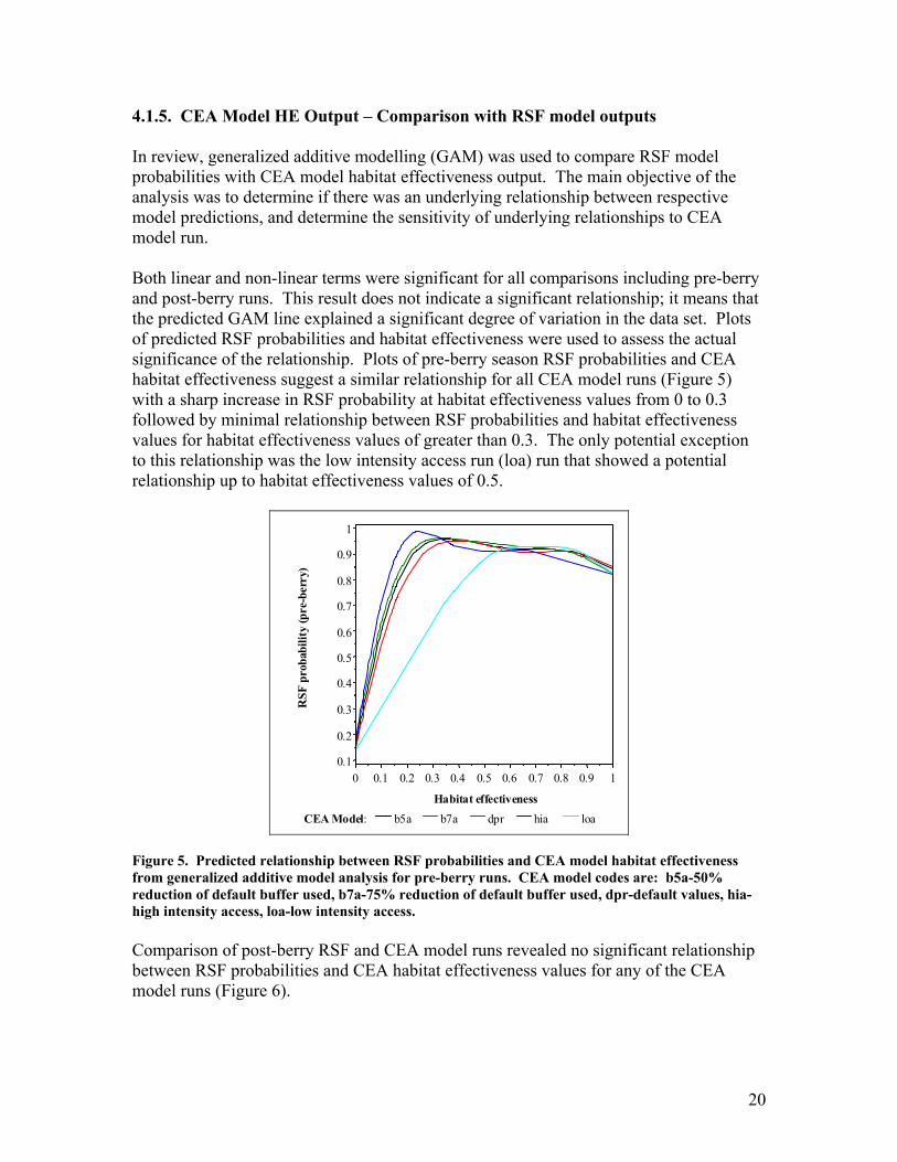
4.1.5. CEA Model HE Output – Comparison with RSF model outputs In review, generalized additive modelling (GAM) was used to compare RSF model probabilities with CEA model habitat effectiveness output. The main objective of the analysis was to determine if there was an underlying relationship between respective model predictions, and determine the sensitivity of underlying relationships to CEA model run. Both linear and non-linear terms were significant for all comparisons including pre-berry and post-berry runs. This result does not indicate a significant relationship; it means that the predicted GAM line explained a significant degree of variation in the data set. Plots of predicted RSF probabilities and habitat effectiveness were used to assess the actual significance of the relationship. Plots of pre-berry season RSF probabilities and CEA habitat effectiveness suggest a similar relationship for all CEA model runs (Figure 5) with a sharp increase in RSF probability at habitat effectiveness values from 0 to 0.3 followed by minimal relationship between RSF probabilities and habitat effectiveness values for habitat effectiveness values of greater than 0.3. The only potential exception to this relationship was the low intensity access run (loa) run that showed a potential relationship up to habitat effectiveness values of 0.5.

CEA Model: b5a b7a dpr hia loa

RSF

pro

babi

lity

(pre

-ber

ry)

0.1

0.2

0.3

0.4

0.5

0.6

0.7

0.8

0.9

1

Habitat effectiveness

0 0.1 0.2 0.3 0.4 0.5 0.6 0.7 0.8 0.9 1

Figure 5. Predicted relationship between RSF probabilities and CEA model habitat effectiveness from generalized additive model analysis for pre-berry runs. CEA model codes are: b5a-50% reduction of default buffer used, b7a-75% reduction of default buffer used, dpr-default values, hia-high intensity access, loa-low intensity access. Comparison of post-berry RSF and CEA model runs revealed no significant relationship between RSF probabilities and CEA habitat effectiveness values for any of the CEA model runs (Figure 6).

20

CEA Model: b5b b7b dpo hib lob

RSF

pro

babi

lity

(pos

t-ber

ry)

0

0.05

0.1

0.15

0.2

0.25

0.3

Habitat effectiveness0 0.1 0.2 0.3 0.4 0.5 0.6 0.7 0.8 0.9 1

Figure 6. Predicted relationship between RSF probabilities and CEA model habitat effectiveness from generalized additive model analysis for post-berry model runs. CEA model codes are: b5b-50% reduction of default buffer used, b7b-75% reduction of default buffer used, dpo-default values, hib-high intensity access, lob-low intensity access.

4.2. Security Area (SA) Analysis Comparisons were made with the assumption that the percentage of secure area in each BMU would be positively correlated with the number of bear identified (per 100 km2) in each BMU using DNA techniques (DDNA), and number of GPS bears (DGPS). Increasing the percentage of secure area should also be correlated with decreasing fragmentation as measured by landscape metrics. Table 12. Total area in each security/usability classification for each BMU.

BMU Secure (km2)

NS-Size (km2)

NS-Human (km2)

Useable (km2)

Unusable (km2)

Total (km2)

% Secure area

Medicine Tent* 107.04 0.37 114.48 221.89 143.89 365.78 29.3%Southesk* 120.25 1.26 0.00 121.51 201.36 322.87 37.2%Whitehorse 133.56 18.66 80.27 232.49 105.39 337.88 39.5%Restless* 102.09 0.49 0.00 102.58 127.41 229.99 44.4%Isaak* 162.48 2.98 2.66 168.12 184.85 352.97 46.0%Fiddle* 136.90 10.44 53.96 201.30 90.13 291.43 47.0%Maskuta 129.39 24.37 97.66 251.42 3.85 255.27 50.7%Gregg 230.83 14.51 128.64 373.98 24.31 398.29 58.0%Upper Rocky * 264.89 1.39 3.91 270.19 161.52 431.71 61.4%Lower Rocky* 297.21 7.01 12.60 316.82 108.09 424.91 70.0%Cardinal 226.18 0.36 31.08 257.62 62.12 319.74 70.7%Brazeau 319.30 7.79 33.80 360.89 39.45 400.34 79.8%Beaverdam 313.67 10.26 47.76 371.69 12.44 384.13 81.7%Pembina 285.48 0.00 31.91 317.39 3.94 321.33 88.8%

* Jasper National Park BMUs

21

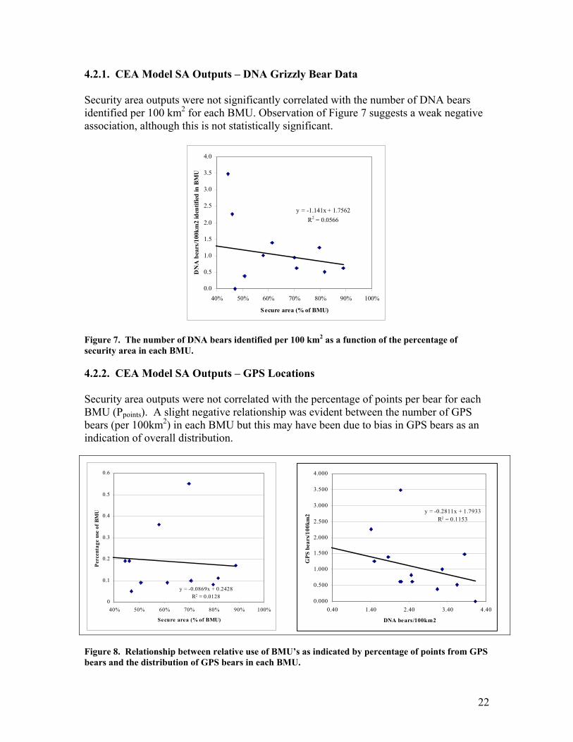
4.2.1. CEA Model SA Outputs – DNA Grizzly Bear Data Security area outputs were not significantly correlated with the number of DNA bears identified per 100 km2 for each BMU. Observation of Figure 7 suggests a weak negative association, although this is not statistically significant.

y = -1.141x + 1.7562R2 = 0.0566

0.0

0.5

1.0

1.5

2.0

2.5

3.0

3.5

4.0

40% 50% 60% 70% 80% 90% 100%

Secure area (% of BMU)

DN

A b

ears

/100

km2

iden

tifie

d in

BM

U

Figure 7. The number of DNA bears identified per 100 km2 as a function of the percentage of security area in each BMU. 4.2.2. CEA Model SA Outputs – GPS Locations Security area outputs were not correlated with the percentage of points per bear for each BMU (Ppoints). A slight negative relationship was evident between the number of GPS bears (per 100km2) in each BMU but this may have been due to bias in GPS bears as an indication of overall distribution.

y = -0.0869x + 0.2428R2 = 0.0128

0

0.1

0.2

0.3

0.4

0.5

0.6

40% 50% 60% 70% 80% 90% 100%

Secure area (% of BMU)

Per

cent

age

use

of B

MU

y = -0.2811x + 1.7933R2 = 0.1153

0.000

0.500

1.000

1.500

2.000

2.500

3.000

3.500

4.000

0.40 1.40 2.40 3.40 4.40

DNA bears/100km2

GPS

bea

rs/1

00km

2

Figure 8. Relationship between relative use of BMU’s as indicated by percentage of points from GPS bears and the distribution of GPS bears in each BMU.

22

5. Discussion and Conclusion The CEA model is not very sensitive to changes in habitat quality between pre- and post-berry seasons. According to this model, the changes between seasons were too subtle to affect a change in habitat effectiveness. The model is highly sensitive to changes in intensity of human use. Changes in human use intensity from low to high resulted in a reduction of habitat effectiveness of one or two categories in all BMUs except the Lower and Upper Rocky BMUs. Using best available data for human use intensity, habitat effectiveness for BMUs in Jasper National Park were closer to those generated using low human use intensity assumptions. Habitat effectiveness for BMUs outside the park, however, was closer to those generated using high human use intensity assumptions. This is likely a result of the lack of motorized access in the park compared with outside the park. As can be expected, decreases in buffer size assumptions resulted in increases in habitat effectiveness. A model’s utility is its ability to be predictive. Comparing model outputs with data gathered from field studies tests the predictive capability of the model. The results of this analysis suggest that predicted distribution and use of BMUs by bears using cumulative effects models is weakly correlated with the distribution of bears identified using DNA methods. It is not correlated with the level of use by GPS bears for each of the BMUs run as indicated by the relative proportion of points in each BMU for each GPS bear. It is negatively correlated with the distribution of GPS bears however this may be an artefact of a biased distribution of GPS bears for the Foothills study area. Security area, a fundamental component of CEA models, is also not significantly correlated with the distribution of DNA bears on the Foothills study area.

One other potential way to compare cumulative effects predictions with the Foothills data was through the use of the RSF models. This method is not perfect in that two models are being compared, making it difficult to discern the actual “truth” given that no model can be considered to be completely unbiased. However, RSF models should be more robust to potential issues with the distribution of GPS bears being indicative of overall distribution. In addition, RSF models consider both bear distribution and habitat selection simultaneously. Therefore, certain results (i.e. RSF model predictions being positively correlated with C.E. habitat effectiveness) would further support some of the preliminary findings from this analysis. The results of the analysis suggest a potential general correspondence between habitat effectiveness and RSF model probabilities at low habitat effectiveness values in the pre-berry season, but no correspondence at higher habitat effectiveness values, or for model runs in the post-berry season. This suggests that habitat effectiveness models and RSF models may agree for the lower range of habitats, but do not seem to have any correspondence for the higher ranges of habitat effectiveness and RSF values. The effectiveness of any model is determined by the quality of the data used in the model and the soundness of the assumptions. With this model, the base habitat map was built on a subjective assessment of habitat quality and assumptions were made on the effects of human use intensity and linear feature buffers on habitat use by bears. Models are also an

23

attempt to simulate the effects of a highly complex environment in which the cumulative effects of environmental, social and individual variations on habitat use are not well understood. For these runs, the model’s failure may not necessarily mean the model lacks validity. The model’s ability to predict grizzly bear use of BMUs may be improved through improvements to the base habitat map or by reassessing the assumptions used. Since these runs, an improved habitat map using an Integrated Decision Tree (IDT) process has been developed. Use of this product as a base habitat map may improve model effectiveness. Ongoing research into the effects of human access and intensity of human use on grizzly bear activity will be used to reassess the assumptions used in the model. The research may also identify other environmental or social factors that affect habitat use by grizzly bears and which may be incorporated into the model.

24

Appendix A

Overview of USDA Grizzly Bear Cumulative Effects Model The CEM is composed of three distinct routines: habitat, disturbance, and mortality. These routines work together to predict habitat effectiveness and mortality risk. Analysis areas are divided into smaller units referred to as Bear Management Units (BMUs). The habitat routine quantifies grizzly bear habitat values. Habitat value incorporates the factors of plant foods, security cover, edge density, and animal food protein sources. The disturbance routine quantifies the effects of disturbance associated with human use and activity on the grizzly bears ability to use a specific habitat. The interaction of habitat value and disturbance determines an area’s habitat effectiveness. The mortality routine provides a relative numeric evaluation of the risk of grizzly bear mortality due to human activity. The CEM uses activity classifications to differentiate between motorized and non-motorized features, and high vs. low levels of human use. Habitat Effectiveness Habitat effectiveness reflects an area’s actual ability to support grizzly bears by comparing an area’s habitat and disturbance components (Gibeau, 1998). Zones of influence, or human use buffer values, are needed in the assessment of habitat effectiveness. The potential for a given area to support bears is compared to the realized ability to support bears once human disturbance is considered (Purves and Doering 1998). The ratio of realized habitat vs. potential habitat determines the habitat effectiveness which is presented as a percentage. Zones of influence are created around areas of human use, depending on the intensity and type of activity. Zones of influence are buffers where it is assumed bears will be affected by human disturbance, and these areas are not included in the calculation of habitat effectiveness. Summary of human use buffer values: Table 1. Zones of Influence (ZOI1) used by Yellowstone 1993, Purves and Doering 1998, Gibeau, 1998. Revised ZOI2 prepared by Mattson 1998 for Yellowstone.

Category ZOI1 (m) Revised ZOI2 (m) Aircraft - Mapped polygons Major development - 5000 Linear motorized/high use 800 500 Linear motorized/low use 800 300 Linear motorized/incidental 800 300 Motorized point diurnal/high 800 1000 Motorized point diurnal/low 800 1000 Motorized point/24-hr 800 1000

25

Category ZOI1 (m) Revised ZOI2 (m) Motorized dispersed/high use - Mapped polygons Motorized dispersed/low use - Mapped polygons Non-motorized linear/high 400 300 Non-motorized linear/low 400 300 Non-motorized point/diurnal 400 500 Non-motorized point/24-hr 400 500 Non-motorized dispersed/high - Mapped polygons Non-motorized dispersed/low - Mapped polygons

The original ZOI values were derived from research conducted by Dave Matson and his colleagues (Mattson et al. 1987) in the Yellowstone Park and were subsequently used by Purves and Doering 1998 and Gibeau 1998. Mattson revised both the ZOI’s and coefficients in September of 1998. A summary of both the old and new coefficients are presented in Table 2. Other researchers have proposed zones of influence (Young 1985) for grizzly bear response to human activities. These include: - 1000m around roads open to four wheeled vehicles (Aune and Stivers 1983 -Rocky

Mountain Front grizzly bear monitoring and investigation); - 1000m around oil and gas drill sites (Harding and Nagy 1980 - Responses of grizzly

bears to hydrocarbon exploration on Richards Island, NorthWest Territories); and - 800m around trails, snowmobile routes, timber activities and campgrounds (Chester

1976- Human wildlife interactions in the Gallatin Range, Yellowstone National Park, 1973-1974).

Human traffic along open roads displaces most grizzly bears from 100m to 900m (Mattson et.al. 1987; McLellan & Shackleton 1988; Aune & Kasworm 1989; Kasworm & Manley 1990; Mace et.al. 1996). McLellan & Shackleton 1988 found that most grizzly bears used open areas near roads less than expected. There was a habitat loss of 58% in the 0-100m DRC and 7% in the 101-250m DRC (distance from road category). This was determined through the observation of 27 radio-collared bears in five separate distance from road categories. Values of high/low human activity: In the Purves and Doering (1998), CEM high levels of human activity is classified as >100 human disturbances/month. The USDA Forest Service Model uses 80 disturbances per month as the division between high and low use. High intensity use for motorized activity restricted to roads, trails, or linear corridors of travel is averaged at 20 or more vehicular disturbances per week (USDA CEM, 1990).

26

Disturbance Coefficients: Disturbance coefficients are rated on a scale from 0-1 based on how grizzly bears would respond to a certain activity. Both Purves and Doering (1998) and Gibeau (1998) based their disturbance coefficients on the Yellowstone ecosystem data. Coefficients from the Yellowstone ecosystem were used because there is no empirical data on human influences in the Canadian Rocky Mountains (Gibeau 1998). Mike Gibeau communicated with Mattson and concurred that the Yellowstone situation is analogous to the three Canadian mountain parks (Gibeau 1998).

Table 2: Coefficients of habitat effectiveness for human features used by Yellowstone 1993, Purves and Doering 1998 and Gibeau 1998. Revised Coefficients were devised for Yellowstone 1998.

Activity Feature Intensity Cover Coefficient Revised Coefficient

Motorized Point High Cover 0.37 0.38 Motorized Point High Non-cover 0.16 0.18 Motorized Point Low Cover 0.73 0.67 Motorized Point Low Non-cover 0.64 0.47 Motorized Line High Cover 0.37 0.45 Motorized Line High Non-cover 0.16 0.21 Motorized Line Low Cover 0.73 0.21 Motorized Line Low Non-cover 0.64 0.19 Motorized Polygon High Cover 0.37 0.48 Motorized Polygon High Non-cover 0.16 0.13 Motorized Polygon Low Cover 0.73 0.84 Motorized Polygon Low Non-cover 0.64 0.66 Non-motorized Point High/diurnal Cover 0.50 0.67 (diurnal) Non-motorized Point High/diurnal Non-cover 0.33 0.47 (diurnal) Non-motorized Point Low/24 hour Cover 0.88 0.38 (24 hour) Non-motorized Point Low/24 hour Non-cover 0.83 0.18 (24 hour) Non-motorized Line High Cover 0.65 0.32 Non-motorized Line High Non-cover 0.56 0.18 Non-motorized Line Low Cover 0.88 0.62 Non-motorized Line Low Non-cover 0.83 0.39 Non-motorized Polygon High Cover 0.50 0.98 Non-motorized Polygon High Non-cover 0.33 0.92 Non-motorized Polygon Low Cover 0.88 0.99 Non-motorized Polygon Low Non-cover 0.83 0.97

In his most recent paper on this topic, Mattson (1998) does not use the term “disturbance coefficient”. Instead, effective habitat productivity is calculated as the product of habitat productivity times coefficient of habitat effectiveness. Coefficients of habitat effectiveness are proportional to the fraction of potential net digested energy that is extracted by bears within a zone of influence. The development of these new coefficients

27

of habitat effectiveness lay on the middle ground between empiricism and informed speculation (Mattson 1998). In order to calculate disturbance coefficients, activities are stratified into groups having similar disturbance potentials. The type of activity is determined by the dominant disturbance element associated with the activity (USDA CEM, 1990). The activities are grouped into the following classifications: 1. Type of activity: motorized, non-motorized, explosive; 2. Nature of activity: point, linear, dispersed; 3. Length of activity: diurnal or 24 hour; and 4. Intensity of activity: high or low. Each activity classification type has a zone of influence (ZOI) calculated for it. The ZOI is computer generated for point and linear activities by creating a buffer zone, where: - values are assigned to each activity type indicating the degree to which habitat within

the ZOI remains effectively usable by bears. - a scale from 0.0 to 1.0 is used based upon how grizzly bears would respond to a given

activity in a 24 hour period. - factors such as habituation to people and avoiding people are incorporated into the

disturbance coefficient (eg. if a bear population has a high level of habituation, the disturbance coefficient would approach 1.0).

The CEM model then multiplies the disturbance coefficient by a corresponding habitat value to determine the habitat effectiveness, a value from 0 to 10. Habitat values represent the inherent quality of an area to support bear use. It incorporates the factors of plant foods, security cover, edge density and animal food protein sources (USDA CEM 1990). Security Areas Security areas are places suitable for individual foraging bouts for adult female grizzlies, free from human disturbance, and of minimum size. They are based on feature, activity, intensity, elevation coverage, and vegetative coverage (Purves and Doering, 1998). Security areas are also based on habitat quality, spacing and connectivity between female home ranges (Gibeau et.al. 1996). Within the Purves and Doering (1998) CEA Model, security areas were arrived at as follows: (these steps were taken from Gibeau et al. 1996): 1. Default buffer distance for high intensity features only: 500m; 2. High intensity classified as 100 disturbances/month; 3. Default minimum polygon size is 9 km²; 4. Elevation cutoff at 2400m according to the Central Rockies Ecosystem Atlas (Komex

1995);

28

5. Vegetative coverage determined by the Central Rockies Ecosystem Atlas (Komex 1995);

6. Ecosites: 1:50,000 scale digital mapping of ecosites; 7. Remove all areas at elevations higher than 2400m, and all non-vegetated areas (ie

rock, ice, and bare soil); 8. All buffer zone areas removed from high human use areas; and 9. Remove all areas less than the determined minimum polygon size. Other approaches to determining core security areas Hamer and Herrero (1983) recorded an average daily foraging radius of 1.2 km for adult female grizzly bears in Cascade Valley. This corresponds closely with empirical data from the Yellowstone ecosystem (Mattson 1993). A minimum size criteria of 4.5 km² was adopted through calculating the area of a circle (πr2), and all polygons less than this calculated 4.5 km² were eliminated from analysis (Gibeau et.al. 1996). In addition to using the 4.5 km² minimum security size, Gibeau 1996 also performed an additional analysis with a minimum security size of 10.1 km². This size was adopted by the US Forest Service for the Flathead National Forest based on empirical work by Mace and Manley (1993). Mattson proposed a different minimum security area size from his research in Yellowstone. He recommended security blocks 28 km² in size, or about 10% of the females home range (Weaver 1996). Mattson may have included an additional 500m buffer zone around security areas because of the higher numbers of people visiting Yellowstone (pers.comm. Gibeau). In 1998 Gibeau and Herrero discarded the minimum security size of 4.5 km² that they had used in 1996, and arrived at a minimum daily area requirement of 9 km². Analysis of 153 daily movements from 14 wary adult females produced a mean daily movement distance of 3.4 km (range 0.2-15.0 km, SE= .22 km). They calculated that the average daily foraging radius was 1.7 km with a 9.0 km² minimum daily area requirement. Through his research Weaver found that 80% of bear locations occurred in blocks of undisturbed habitat 9 km² or more in size, or about 7% of the average home range (Weaver 1996). Young (1985), in his research in the Lewis and Clark National Forest, determined minimum space requirements by finding the density of adult female grizzlies in the core study BMU, and then extrapolating the densities to the other BMUs. He found that the minimum space required to support each adult female grizzly on concentrated use spring range was 84 km². Linkage Zones

Linkage zones identify possible movement corridors for grizzly bears considering the influence of human activity. They are based on access density (line features such as roads and tracks), developed human use sites (point and polygon features), and presence of hiding cover and riparian areas. The basis of the LZP model is that human

29

development is the primary influence upon grizzly bear distribution, not food availability (Gibeau et.al. 1996). This assumption has yet to be tested. The major assumption of the LZP is that it accurately reflects human use at a landscape scale (Gibeau et.al. 1996). To run the LZP model, a number of parameters are needed: access density categories, high intensity human use cutoff values and scores, developed site buffer sizes, distances and scores, riparian area scores, and the analysis grid size. The linkage zone model was originated by Servheen (1993), and the following scores and procedures are taken from his research.

Arriving at the LZP model: 1. Access Density: The default value for high intensity human use is 100 disturbances/month. Those features that are greater than this cutoff value are used to determine the access density. The lower the score the better the linkage zone is for the bear. Total Length of Access Score < or = 0 km 2 > 0 and <or = 1.61 km 3 > 1.61 km and < or = 3.22 km 4 > 3.22 km 5 2. Developed Sites: Developed sites are buffered according to use. High intensity sites (> 100 disturbances/month) have a buffer size of 240m, while low intensity sites (< 100 disturbances/month) have buffers of 120m. Distance to Nearest Buffer Score 0 m (within a buffer) 6 > 0 and < or = 100 m 5 > 100 m and < or = 200 m 4 > 200 m 2 3. Hiding Cover: Servheen assumed that areas more than 50m from cover are not used frequently by bears and have a greater mortality rate (Gibeau et.al., 1996). Distance to Nearest Cover Score 0 m (within cover) 2 > 0 m and < or = 50 m (edge) 3 > 50 m (non-cover) 5

30

4. Riparian Areas: According to Servheen, riparian areas must have high amounts of bear foods, provide opportunities for movement, and have broad wet site vegetation associations. 50m on either side of riparian areas were considered to provide the same attributes as riparian areas. All stream channels were assigned a 100m buffer to be included in riparian habitats (Gibeau et.al., 1996). Score Inside a riparian area 1 Outside a riparian area 2 Within the CEA model, the sum of all scores from the above four layers provides a danger score, with 18 being the highest human influence. Comments on Thresholds and Landscape Conditions In 1996 Mike Gibeau commented that “the actual response of individual grizzly bears to varying levels of habitat effectiveness has not yet been empirically determined. Currently, there are no clearly defined habitat effectiveness thresholds beyond which grizzly bears are eliminated” (Gibeau et.al. 1996). Mattson (1993), considers adequate security for grizzly bears to be at the 57% level. Target levels of 60-67% are being used by Mace and Waller in their research (1997) and were set by interagency managers for the Northern Continental Divide grizzly bear ecosystem in northwest Montana (Gibeau and Herrero, 1998). In a more recent article by Gibeau: “Grizzly bear habitat effectiveness model for Banff, Yoho, and Kootenay National Parks, Canada”, 1998, he sums up the habitat effectiveness debate:

“There has been considerable discourse regarding habitat threshold levels beyond which grizzly bears are eliminated. In the U.S., researchers have been working towards establishing meaningful ecological thresholds, but how to do this remains unclear…In the case of the grizzly bear in U.S. and Canada, the implications of being wrong have serious consequences: extinction. If the threshold were set at 80% habitat effectiveness, would a manager be comfortable with a 20% chance of being wrong?”

31

References Bio A.M.F., R. Alkemade, A. Barendregt. 1998. Determining alternative models for

vegetation response analysis: a non-parametric approach. Journal of Vegetation Science 9:5-16.

Gibeau, M.L., S. Herrero, J.L. Kansas, and B.Benn. 1996. Grizzly bear population and

habitat status in Banff National Park: A report to the Banff Bow Valley Task Force. 61pp.

Gibeau, M.L. and S. Herrero. 1998. Managing for grizzly bear security areas in Banff

National Park and the Central Canadian Rocky Mountains. International Conference on Bear Research and Management 11:000-000. 16pp.

Gibeau, M.L. 1998. Grizzly bear habitat effectiveness model for Banff, Yoho and

Kootenay National Parks, Canada. Ursus 10: 235-241. Hastie T.J., R.J. Tibshirani. 1990. Generalized additive models. Chapman and Hall. New

York. Herrero, S. and J. Herrero. 1996. Cheviot Mine Project: Specific and Cumulative

Environmental Effects Analysis for Mammalian Carnivores. BIOS Environmental Research and Planning Associates Ltd., Calgary, AB. 122pp.

Komex International. 1995. Atlas of the Central Rockies Ecosystem. Rep. to the

Central Rockies Ecosystem Interagency Liaison Group. Calgary, AB. 49pp. Mace and T.L. Manley. 1993. South Park Flathead River grizzly project: Progress

Report for 1992. Montana Dept. of Fish, Wildlife and Parks. 34 pp. Mace, R.D. and J.S. Waller. 1997. Final report: grizzly bear ecology in the Swan

Mountains. Montana Fish, Wildlife, and Parks Department, Helena, Montana. 191pp.

Mattson, D.J. 1993. Background and proposed standards for managing grizzly bear

habitat security in the Yellowstone ecosystem. Cooperative Park Studies Unit report. University of Idaho, Moscow, Idaho. 17pp.

Mattson, D. Coefficients of productivity for Yellowstone’s grizzly bear habitat. 1998.

Forest and Rangeland Ecosystem Science Centre and Department of Fish and Wildlife Resources, University of Idaho, Moscow, ID. 85pp.

McLellan, B.N. and D.M. Shackleton. 1988. Grizzly bears and resource extraction

industries: effects of roads on behaviour, habitat use, and demography. J.Appl.Ecol. 25: 451-460.

32

33

Otis D.L., G.C. White. 1999. Autocorrelation of estimates and the analysis of radiotracking data. J. Wildl. Manage. 63(3):1039-1043.

Purves, H and C. Doering. 1998. Jasper National Park Cumulative Effects Assessment

(CEA) Application for Grizzly Bears: Version 1. 59pp. SAS Institute. 2000. The SAS System for Windows. Version 8.1. Cary NC: The SAS

Institute. Servheen, C. and P. Sandstrom. 1993. Human activities and linkage zones for grizzly

bears in the Swan-Clearwater Valleys, Montana. U.S. Fish and Wildlife Service, Missoula, MT. 28pp.

USDA Forest Service. 1990. CEM- A model for assessing effects on grizzly bears. U.S.

Department of Agriculture Forest Service, Missoula, Montana. 24pp. Weaver, J.L., P.C. Paquet, and L.F. Ruggiero. 1996. Resilience and conservation of

large carnivores in the Rocky Mountains. Conservation Biology 10: 964-976. Young, D.L. 1985. Cumulative effects analysis of grizzly bear habitat on the Lewis and

Clark National Forest. Grizzly Bear Habitat Symposium, Missoula, MT, April 30-May 2. 5pp.

Zar J.H. 1996. Biostatistical analysis. Prentice-Hall. London., 662 p. Personal Communication: Gibeau, M. Parks Canada, Banff National Park. Banff, Alberta