A MODEL OF SECULAR STAGNATION

Gauti B. Eggertsson and Neil R. Mehrotra

Brown University

PortugalJune, 2015

1 / 47

SECULAR STAGNATION HYPOTHESIS

I wonder if a set of older ideas . . . under the phrase secularstagnation are not profoundly important in understanding Japan’sexperience, and may not be without relevance to America’sexperience — Lawrence Summers

Original hypothesis:

I Alvin Hansen (1938)I Reduction in population growth and investment opportunitiesI Concerns about insufficient demand ended with WWII and

subsequent baby boom

Secular stagnation resurrected:

I Lawrence Summers (2013)I Highly persistent decline in the natural rate of interestI Chronically binding zero lower bound

2 / 47

WHY ARE WE SO CONFIDENT INTEREST RATES

WILL RISE SOON?

Interest rates in the US during the Great Depression:

I Started falling in 1929I Reached zero in 1933I Interest rates only started increasing in 1947

Started dropping in Japan in 1994:I Remains at zero today

Why are we so confident interest rates are increasing in the next fewyears?Wanted: A model that allows for long-lasting slumps.

3 / 47

SHORTCOMINGS OF SOME EXISTING MODELS

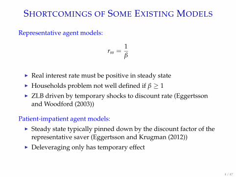
Representative agent models:

rss =1β

I Real interest rate must be positive in steady stateI Households problem not well defined if β ≥ 1I ZLB driven by temporary shocks to discount rate (Eggertsson

and Woodford (2003))

Patient-impatient agent models:I Steady state typically pinned down by the discount factor of the

representative saver (Eggertsson and Krugman (2012))I Deleveraging only has temporary effect

4 / 47

QUESTIONS

Question 1I Can we formalize the idea of secular stagnation?

Question 2I "What facts, exactly, is this meant to capture"I Answer:I (i) Resources are underutilized ("unemployment").I (ii) Short-term risk-free nominal interest rates are at zero and the

CB want to cut them more.I (iii) This situation can last for an arbitrarily long time.

5 / 47

OUTLINE FOR PRESENTATION

1. Model(1958) OLG endowment economy without capital – Negativeshort-term real interest rate can be triggered by:

I Deleveraging shockI Slowdown in population growthI Increase in income inequalityI Fall in relative price of investment

I Endogenous production–Stagnation steady stateI Permanently binding zero lower boundI Low inflation or deflationI Permanent shortfall in output from potential

2. Policy options

3. Capital

4. Conclusions6 / 47

ECONOMIC ENVIRONMENT

ENDOWMENT ECONOMY

I Time: t = 0, 1, 2, ...

I Goods: consumption good (c)

I Agents: 3-generations: iε {y, m, o}

I Assets: riskless bonds (Bi)

I Technology: exogenous borrowing constraint D

7 / 47

HOUSEHOLDS

Objective function:

maxCy

t,,Cmt+1,Co

t+2

U = Et

{log(

Cyt

)+ β log

(Cm

t+1)+ β2 log

(Co

t+2)}

Budget constraints:

Cyt = By

t

Cmt+1 = Ym

t+1 − (1 + rt)Byt + Bm

t+1

Cot+2 = Yo

t+2 − (1 + rt+1)Bmt+1

(1 + rt)Bit ≤ Dt

8 / 47

CONSUMPTION AND SAVING

Credit-constrained youngest generation:

Cyt = By

t =Dt

1 + rt

Saving by the middle generation:

1Cm

t= βEt

1 + rt

Cot+1

Spending by the old:

Cot = Yo

t − (1 + rt−1)Bmt−1

9 / 47

DETERMINATION OF THE REAL INTEREST RATE

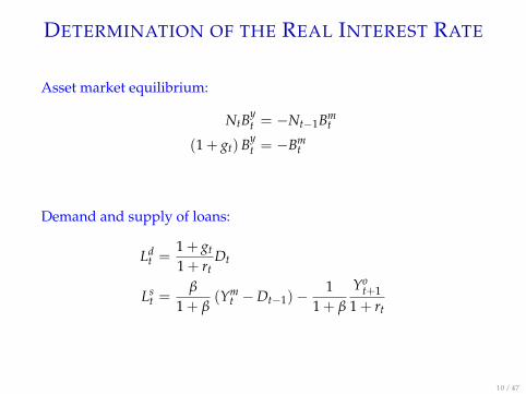
Asset market equilibrium:

NtByt = −Nt−1Bm

t

(1 + gt)Byt = −Bm

t

Demand and supply of loans:

Ldt =

1 + gt

1 + rtDt

Lst =

β

1 + β(Ym

t −Dt−1)−1

1 + β

Yot+1

1 + rt

10 / 47

DETERMINATION OF THE REAL INTEREST RATE

Expression for the real interest rate (perfect foresight):

1 + rt =1 + β

β

(1 + gt)Dt

Ymt −Dt−1

+1β

Yot+1

Ymt −Dt−1

Determinants of the real interest rate:I Tighter collateral constraint reduces the real interest rateI Lower rate of population growth reduces the real interest rateI Higher middle age income reduces real interest rateI Higher old income increases real interest rate

11 / 47

EFFECT OF A DELEVERAGING SHOCK

Impact effect:I Collateral constraint tightens from Dh to Dl

I Reduction in the loan demand and fall in real rateI Akin to Eggertsson and Krugman (2012)

Delayed effect:I Next period, a shift out in loan supplyI Further reduction in real interest rateI Novel effect from Eggertsson and Krugman (2012)I Potentially powerful propagation mechanism

12 / 47

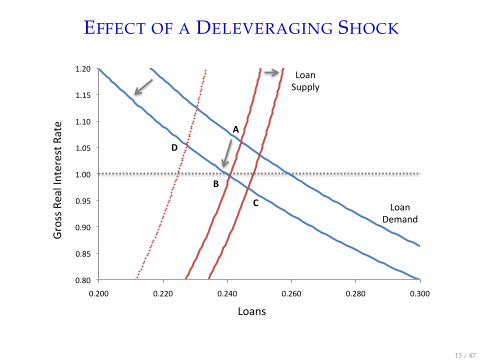
EFFECT OF A DELEVERAGING SHOCK

0.80  

0.85  

0.90  

0.95  

1.00  

1.05  

1.10  

1.15  

1.20  

0.200   0.220   0.240   0.260   0.280   0.300  

Loans  

Gross  Real  Interest  R

ate  

Loan  Supply  

Loan  Demand  

A  

B  

C  

D  

13 / 47

INCOME INEQUALITY

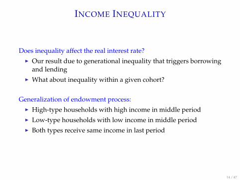
Does inequality affect the real interest rate?I Our result due to generational inequality that triggers borrowing

and lendingI What about inequality within a given cohort?

Generalization of endowment process:I High-type households with high income in middle periodI Low-type households with low income in middle periodI Both types receive same income in last period

14 / 47

INCOME INEQUALITY AND REAL INTEREST

RATE

Credit constrained middle income:I Fraction ηs of middle income households are credit constrainedI True for low enough income in middle generation and high

enough income in retirementI Fraction 1− ηs lend to both young and constrained

middle-generation households

Expression for the real interest rate:

1 + rt =1 + β

β

(1 + gt + ηs)Dt

(1− ηs)(

Ym,ht −Dt−1

) +1

β (1− ηs)

Yot+1(

Ym,ht −Dt−1

)

15 / 47

PRICE LEVEL DETERMINATION: WOODFORD’S

CASHLESS LIMITEuler equation for nominal bonds:

1Cm

t= βEt

1Co

t+1(1 + it)

Pt

Pt+1

it ≥ 0

The ZLB implies a bound on steady state inflation:

Π̄ ≥ 11 + r

I If steady state real rate is negative then steady state inflationmust be positive

I No steady state with zero inflationI But what happens when prices are NOT flexible and the central

bank does not tolerate inflation?16 / 47

OUTLINE FOR PRESENTATION

1. Model

I Endowment economy

I Endogenous production

2. Monetary and fiscal policy

3. Capital

4. Conclusions

17 / 47

ENDOGENOUS PRODUCTION

There are Nt−1 firms with production function

Yt = Lαt

I Labor only factor of production (capital coming up)I Firms take prices and wages as given

Labor supply:I Constant inelastic labor supply from householdsI Assume only middle-generation household supplies laborI Possibility of unemployment due to wage rigidity

18 / 47

AGGREGATE SUPPLY - FULL EMPLOYMENTOutput and labor demand:

Yt = Lαt

Wt

Pt= αLα−1

t

Labor supply:

Lt = L̄

I Implies a constant market clearing real wage W̄ = αL̄α−1

I Implies a constant full-employment level of output: Yf = L̄α

I Again, analogous to the endowment economy, steady state hasto be consistent Π̄ ≥ 1

1+r .

19 / 47

DOWNWARD NOMINAL WAGE RIGIDITY

Partial wage adjustment:

Wt = max{

W̃t, Wflex}

where W̃t = γWt−1 + (1− γ)Wflex

Wage rigidity and unemployment:

I W̃t is a wage normI Wflex = PtαL̄α−1 is the market clearing wage.I If real wages exceed market clearing level, employment is

rationedI Unemployment: Ut = L̄− Lt

I Similar assumption in Kocherlakota (2013) and Schmitt-Groheand Uribe (2013)

20 / 47

THE GOVERNMENT

Government sets inflation at Π = Π∗. It can always achieve thistarget except if it implies negative it.

Πt = Π∗ and it ≥ 0.

If Πt = Π∗ imples it < 0 then

it = 0 and Πt < Π∗

Implementation?

1 + it = max(1, (1 + i∗)(Πt

Π∗)φπ )

21 / 47

ANALYZING THE MODEL

Will analyze the steady state of the modelI A constant solution for (Π, Y, i, r) that solves the equations of the

modelI Reflect a permanent recession (or not).I Will look suspiciously similar to a old fashion IS/LM model.

Bug, feature?I Key weakness: Wage setting is reduced form. Have done Calvo

prices, and other variations. Most important thing: Long-runtradeoff between inflation and output.

22 / 47

PROPOSITION 1: CHARACTERIZATION

The steady state of the model is four numbers (Y, Π, i, r) that satisfy:

Y =(1 + β)(1 + g)

β

D1 + r

+ D (1)

1 + r =1 + i

Π(2)

Π = Π∗ or i = 0 AND Π < Π∗ (3)

Y =

Yf if Π ≥ 1

Yf(

1− γΠ

1−γ

) α1−α

otherwise(4)

23 / 47

DEFINITIONS

Definition The natural level of output is (Friedman (1968))

Yf ≡ L̄α

Definition The natural rate of interest is (Wicksell (1998))

1 + rf ≡ (1 + β)(1 + g)β

DYf −D

Assumption Π∗ ≥ 1

24 / 47

LEMMA ON POSSIBILITIES

Given our assumed policy commitment: There are three possibilities,label them Cases I, II and III.

I Case I (normal equilibrium) Π = Π∗ i > 0.I Case II (full employment ZLB) Π 6= Π∗, Π∗ > Π > 1, i = 0.I Case III (secular stagnation) Π 6= Π∗, Π < 1, i = 0.

25 / 47

LEMMA ON CHARACTERIZATION

I In Case I: Π = Π∗

Y = Yf , 1 + r = 1 + rf , 1 + i = (1 + rf )Π∗

I In Case II: Π∗ > Π > 1

Y = Yf , 1 + r = 1 + rf , Π = (1 + rf )−1 , i = 0

I In Case III: Π < 1.

Y− Yf = ψ

(1

1 + r− 1

1 + rf

), i = 0

Y = Yf

(1− γ

Π1− γ

) α1−α

1 + r =1Π

where ψ ≡ (1+β)(1+g)β D > 0

26 / 47

PROPOSITIONS

I Prop 1: Suppose rf > 0, Π∗ = 1. Then, there exists a normalequilibrium (Case I) with Π = 1, r = i = rf , Y = Yf .

I Prop 2: Suppose rf < 0, Π∗ = 1. Then a normal equilibrium doesnot exist.

I Prop 3: Suppose rf < 0 and Π∗ = 1. Then there exists a secularstagnation equilibrium (Case III). This is the unique equilibriumin this case.

27 / 47

FULL EMPLOYMENT STEADY STATE

0.80  

0.85  

0.90  

0.95  

1.00  

1.05  

1.10  

1.15  

1.20  

0.80   0.85   0.90   0.95   1.00   1.05   1.10  

Output  

Gross  Infl

a5on

 Rate  

Aggregate  Supply  

FE  Steady  State  

Aggregate  Demand  

Parameter Values

28 / 47

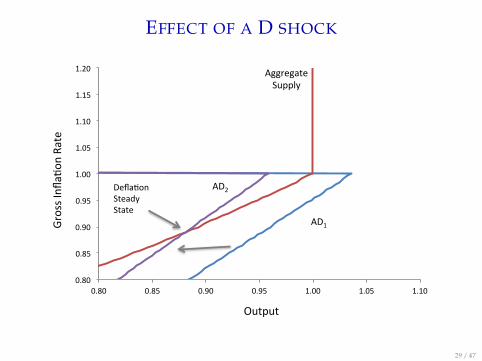
EFFECT OF A D SHOCK

0.80  

0.85  

0.90  

0.95  

1.00  

1.05  

1.10  

1.15  

1.20  

0.80   0.85   0.90   0.95   1.00   1.05   1.10  

Output  

Gross  Infl

a5on

 Rate  

Aggregate  Supply  

Defla5on  Steady  State  

AD1  

AD2  

29 / 47

PROPERTIES OF THE STAGNATION STEADY

STATE

Long slump:I Binding zero lower bound so long as natural rate is negativeI Deflation raises real wages above market-clearing levelI Output persistently below full-employment level

Existence and stability:I Secular stagnation steady state exists so long as γ > 0I Prop 4: If Π∗ = 1, secular stagnation steady state is determinate.

(There is a unique bounded solution local to ss)I Contrast to deflation steady state emphasized in Benhabib,

Schmitt-Grohe and Uribe (2001)I Can do comparative statics!

30 / 47

MECHANISM OF ADJUSTMENT BACK TO FULL

EMPLOYMENT

Financial shockI Reverts back to original level, you get back to where you startedI Observation: Policy been going into the opposite direction.

Wages become more flexibleI Works in the wrong direction: Paradox of flexibilityI Output drops by more as wages become more flexible.I Same result if you add more forward looking behavior in wage

setting: More deflation, bigger drop in output.

Labor participation decreasesI Reduces Wflex and increases output.I But reduces Yf : Paradox of toil.

31 / 47

INCREASING WAGE FLEXIBILITY

0.75  

0.80  

0.85  

0.90  

0.95  

1.00  

1.05  

1.10  

1.15  

1.20  

0.70   0.75   0.80   0.85   0.90   0.95   1.00   1.05   1.10  

Output  

Gross  Infl

a6on

 Rate  

AS1   Higher  Wage  Flexibility  Steady  State  

AD2  

Defla6on  Steady  State  

AS2  

32 / 47

REDUCTION IN LABOR SUPPLY (HYSTERESIS)

0.75  

0.80  

0.85  

0.90  

0.95  

1.00  

1.05  

1.10  

1.15  

1.20  

0.70   0.75   0.80   0.85   0.90   0.95   1.00   1.05   1.10  

Output  

Gross  Infl

a6on

 Rate  

AS1  

High  Produc6vity  Steady  State  

AD2  

Defla6on  Steady  State  

AS2  

33 / 47

MONETARY POLICY RESPONSES

Forward guidance:I Extended commitment to keep nominal rates low?I Ineffective if households/firms expect rates to remain low

indefinitely

Raising the inflation target:I For sufficiently high inflation target, full employment steady

state existsI Timidity trap (Krugman (2014))I Multiple determinate steady statesI Monetary policy not as powerful as in earlier models because no

way to exclude secular stagnation

34 / 47

RAISING THE INFLATION TARGET

PropositionSuppose rf < 0 and Π∗ > 1

1+rf . Then three equilibria in themodel are possible - all three cases from the Lemma onpossibilities.

35 / 47

RAISING THE INFLATION TARGET

0.80  

0.85  

0.90  

0.95  

1.00  

1.05  

1.10  

1.15  

1.20  

0.80   0.85   0.90   0.95   1.00   1.05   1.10  

Output  

Gross  Infl

a5on

 Rate  

Aggregate  Supply  

Full  Employment  Steady  State  

AD2  

AD3  

Defla5on  Steady  State  

AD1  

36 / 47

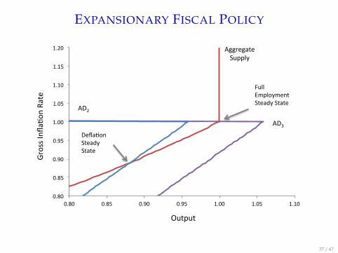
EXPANSIONARY FISCAL POLICY

0.80  

0.85  

0.90  

0.95  

1.00  

1.05  

1.10  

1.15  

1.20  

0.80   0.85   0.90   0.95   1.00   1.05   1.10  

Output  

Gross  Infl

a5on

 Rate  

Aggregate  Supply  

Full  Employment  Steady  State  

AD2  

AD3  

Defla5on  Steady  State  

37 / 47

FISCAL POLICY

Fiscal policy and the real interest rate:

Ldt =

1 + gt

1 + rtDt + Bg

t

Lst =

β

1 + β(Ym

t −Dt−1 − Tmt )−

11 + β

Yot+1 − To

t+11 + rt

Government budget constraint:

Bgt + Ty

t (1 + gt) + Tmt +

11 + gt−1

Tot = Gt +

1 + rt

1 + gt−1Bg

t−1

Fiscal instruments:

Gt, Bgt , Ty

t , Tmt , To

t

38 / 47

TEMPORARY INCREASE IN PUBLIC DEBT

Under constant population and set Gt = Tyt = Bg

t−1 = 0:

Tmt = −Bg

t

Tot+1 = (1 + rt)Bg

t

Implications for natural rate:I Loan demand and loan supply effects cancel outI Temporary increases in public debt ineffective in raising real rateI Temporary monetary expansion equivalent to temporary

expansion in public debt at the zero lower boundI Effect of an increase in public debt depends on beliefs about

future fiscal policy

39 / 47

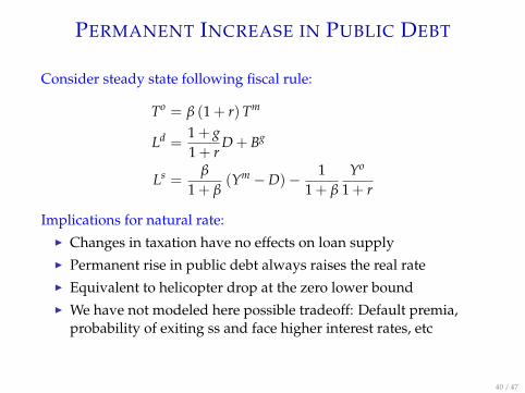
PERMANENT INCREASE IN PUBLIC DEBT

Consider steady state following fiscal rule:

To = β (1 + r)Tm

Ld =1 + g1 + r

D + Bg

Ls =β

1 + β(Ym −D)− 1

1 + β

Yo

1 + r

Implications for natural rate:I Changes in taxation have no effects on loan supplyI Permanent rise in public debt always raises the real rateI Equivalent to helicopter drop at the zero lower boundI We have not modeled here possible tradeoff: Default premia,

probability of exiting ss and face higher interest rates, etc

40 / 47

GOVERNMENT PURCHASES MULTIPLIER

Slope of the AD and AS curves:

ψ =1 + β

β(1 + g)D

κ =1− α

α

1− γ

γ

Purchases multiplier at the zero lower bound:

Financing Multiplier Value

Increase in public debt 1+ββ

11−κψ > 2

Tax on young generation 0 0

Tax on middle generation 11−κψ > 1

Tax on old generation − 1+gβ

11−κψ < 0

41 / 47

HOUSEHOLDS

Objective function:

maxCy

t,,Cmt+1,Co

t+2

U = Et

{log(

Cyt

)+ β log

(Cm

t+1)+ β2 log

(Co

t+2)}

Budget constraints:

Cyt = By

t

Cmt+1 + pk

t+1Kt+1 + (1 + rt)Byt = wt+1Lt+1 + rk

t+1Kt+1 + Bmt+1

Cot+2 + (1 + rt+1)Bm

t+1 = pkt+2 (1− δ)Kt+1

Dynamic Efficiency

42 / 47

CHARACTERIZATION

Capital supply (perfect foresight):(pk

t − rkt

) 1Cm

t= βpk

t+1 (1− δ)1

Cot+1

Loan supply and demand:

Ldt =

1 + gt

1 + rtDt

Lst =

β

1 + β(Yt −Dt−1)−

β

1 + β

(pk

t + pkt+1

1− δ

β (1 + rt)

)Kt

43 / 47

CAPITAL AND SECULAR STAGNATION

Rental rate and real interest rate:

rkt = pk

t − pkt+1

1− δ

1 + rt≥ 0

rss ≥ −δ

I Negative real rate now constrained by fact that rental rate mustbe positive

Relative price of capital goods:I Decline in relative price of capital goodsI Need less savings to build the same capital stockI –> downward pressure on the real interest rate.I Global decline in price of capital goods (Karabarbounis and

Neiman, 2014)

Land

44 / 47

EFFECT OF A SHOCK TO PRICE OF CAPITAL

GOODS

0.80  

0.85  

0.90  

0.95  

1.00  

1.05  

1.10  

1.15  

1.20  

0.090   0.100   0.110   0.120   0.130   0.140   0.150  

Loans  

Gross  Real  Interest  R

ate  

Loan  Supply  

Loan  Demand  

45 / 47

PARADOX OF THRIFT

EFFECT OF A DISCOUNT RATE SHOCK

Positive natural rate

0.90  

0.95  

1.00  

1.05  

1.10  

1.15  

1.20  

0.90   0.95   1.00   1.05   1.10  

Output  

Gross  Infla4o

n  Ra

te  

AS1  

Normal  Equilibrium  

AD2   AD1  

Austerity  Equilibrium  

Negative natural rate

0.80  

0.85  

0.90  

0.95  

1.00  

1.05  

1.10  

0.70   0.75   0.80   0.85   0.90   0.95   1.00  

Output  

Gross  Infla5o

n  Ra

te  

AD2   AD1   AS2  

Secular  Stagna5on  Equilibrium  

Austerity  Equilibrium  

46 / 47

CONCLUSIONS

Policy implications:I Higher inflation target neededI Limits to forward guidanceI Role for fiscal policyI In absence of policy, not an obvious mechanism for adjustment.I Pay as you go social security, increase retirement age

Key takeaways:I NOT that we will stay in a slump foreverI Slump of arbitrary durationI OLG framework to model interest rates

47 / 47