gate-users guide v8 - opengatecollaboration.org · however these packages are quite complex and...

Users Guide V8.0From Wiki OpenGATE

Introduction

Contents1 General Concept2 Imaging applications3 Radiotherapy and Dosimetry applications4 Thermal therapy application5 Parallel Computing

General ConceptGetting startedDefining a geometryMaterialsSetting up the physicsCut and Variance Reduction TechniquesSource and particle managementVoxelized Source and PhantomTools to Interact with the Simulation : ActorsHow to run GateVisualization

Imaging applications

Defining a system : scanner, CT, PET, SPECT, OpticalSensitive detector conceptDigitizer and detector modelingData output managementGenerating and tracking optical photonsList of examples (https://github.com/OpenGATE/GateContrib/tree/master/imaging)

Radiotherapy and Dosimetry applicationsGeneral ConceptBeam modellingList of exercises and examples (https://github.com/OpenGATE/GateContrib/tree/master/dosimetry)

Thermal therapy applicationNanoparticle mediated hyperthermia

Parallel ComputingHow to use Gate on a ClusterHow to use Gate on a GPU

Retrieved from "http://wiki.opengatecollaboration.org/index.php?title=Users_Guide_V8.0&oldid=910"

This page was last modified on 28 March 2017, at 13:14.

UsersGuideV8.0:IntroductionFrom Wiki OpenGATE

Geant4 Application for Emission Tomography: a simulation toolkit for PET and SPECT

OpenGATE Collaboration

http://www.opengatecollaboration.org

Contents1 Authors2 The GATE mailing list3 Forewords4 Member institutes of the OpenGATE Collaboration (May 2015):5 Overview

Authors

OpenGATE spokesperson: I. Buvat (IMIV UMR1023 Inserm-CEA-Université Paris Sud, ERL 9218 CNRS Orsay)

OpenGATE technical coordinator: S. Jan (IMIV UMR1023 Inserm-CEA-Université Paris Sud, ERL 9218 CNRS Orsay)

Editorial board at the time of the first Users Guide version (2004) S. Glick (UMASS), S. Kerhoas (CEA Saclay), F. Mayet (CNRS-LPSC Grenoble)

Authors of the first edition (2004) : S. Jan, G. Santin, D. Strul, S. Staelens, K. Assié, D. Autret, S. Avner, R. Barbier, M. Bardiès, P. M. Bloomfield, D.Brasse, V. Breton, P. Bruyndonckx, I. Buvat, A. F. Chatziioannou, Y. Choi, Y. H. Chung, C. Comtat, D. Donnarieix, L. Ferrer, S. J. Glick, C. J. Groiselle, D.Guez, P.-F. Honore, S. Kerhoas-Cavata, A. S. Kirov, V. Kohli, M. Koole, M. Krieguer, D. J. van der Laan, F. Lamare, G. Largeron, C. Lartizien, D. Lazaro,M. C. Maas, L. Maigne, F. Mayet, F. Melot, C. Merheb, E. Pennacchio, J. Perez, U. Pietrzyk, F. R. Rannou, M. Rey, D. R. Schaart, C. R. Schmidtlein, L.Simon, T. Y. Song, J.-M. Vieira, D. Visvikis, R. Van de Walle, E. Wieers, C. Morel

Special Thanks: Geant4 Collaboration and LOW energy WG

The GATE mailing list

You are encouraged to participate in the dialog and post your suggestions, questions and answers to colleagues' questions on the gate-users mailing list, theGATE mailing list for users. You can subscribe to the gate-users mailing list, by registering at the GATE web site: http://www.opengatecollaboration.org

If you have a question, it is very likely that it has already been asked and answered, and is now stored in the archives. Please use the search engine to see ifyour question has already been answered before sending a mail to the GATE-users .

Forewords

Monte Carlo simulation is an essential tool in emission tomography to assist in the design of new medical imaging devices, assess new implementations ofimage reconstruction algorithms and/or scatter correction techniques, and optimise scan protocols. Although dedicated Monte Carlo codes have beendeveloped for Positron Emission Tomography (PET) and for Single Photon Emission Computerized Tomography (SPECT), these tools suffer from a varietyof drawbacks and limitations in terms of validation, accuracy, and/or support (Buvat). On the other hand, accurate and versatile simulation codes such asGEANT3 (G3), EGS4, MCNP, and GEANT4 have been written for high energy physics. They all include well-validated physics models, geometry modelingtools, and efficient visualization utilities. However these packages are quite complex and necessitate a steep learning curve.

GATE, the GEANT4 Application for Emission Tomography (MIC02, Siena02, ITBS02, GATE, encapsulates the GEANT4 libraries in order to achieve amodular, versatile, scripted simulation toolkit adapted to the field of nuclear medicine. In particular, GATE provides the capability for modeling time-dependent phenomena such as detector movements or source decay kinetics, thus allowing the simulation of time curves under realistic acquisitionconditions.

GATE was developed within the OpenGATE Collaboration with the objective to provide the academic community with a free software, general-purpose,GEANT4-based simulation platform for emission tomography. The collaboration currently includes 21 laboratories fully dedicated to the task of improving,documenting, and testing GATE thoroughly against most of the imaging systems commercially available in PET and SPECT (Staelens, Lazaro).

Particular attention was paid to provide meaningful documentation with the simulation software package, including installation and user's guides, and a listof FAQs. This will hopefully make possible the long term support and continuity of GATE, which we intend to propose as a new standard for Monte Carlosimulation in nuclear medicine.

In name of the OpenGATE Collaboration

Christian MOREL CPPM CNRS/IN2P3, Marseille

Member institutes of the OpenGATE Collaboration (May 2015):

CNRS Laboratory of Corpuscular Physics @ Clermont-Ferrand (LPC)CNRS Centre de Physique des Particules de Marseille (CPPM), MarseilleCNRS Imaging and Modelling in Neurobiology and Cancerology lab @ Orsay (IMNC), OrsayCNRS IRES, Centre Pluridisciplinaire Hubert Curien (CPHC) @ StrasbourgCNRS Laboratoire de Physique Subatomique et des technologies associées (SUBATECH), NantesINSERM - CNRS CREATIS lab @ LyonU892 INSERM @ NantesLATIM, U1101 INSERM, Brest

IMIV, UMR1023 Inserm-CEA-Université Paris Sud, ERL 9218 CNRS, Service Hospitalier Frédéric Joliot (SHFJ), OrsaySungkyunkwan University School of Medicine (DMN), SeoulForschungszentrum-Juelich (IME)Memorial Sloan-Kettering Cancer Center (Department of Medical Physics), New YorkUniversity of Athens (IASA)Delft University of Technology (IRI)UC Davis, CaliforniaMedAustron, Wiener NeustadtMedical University Vienna, WienUMR 1037 INSERM/UPS, Toulouse

Overview

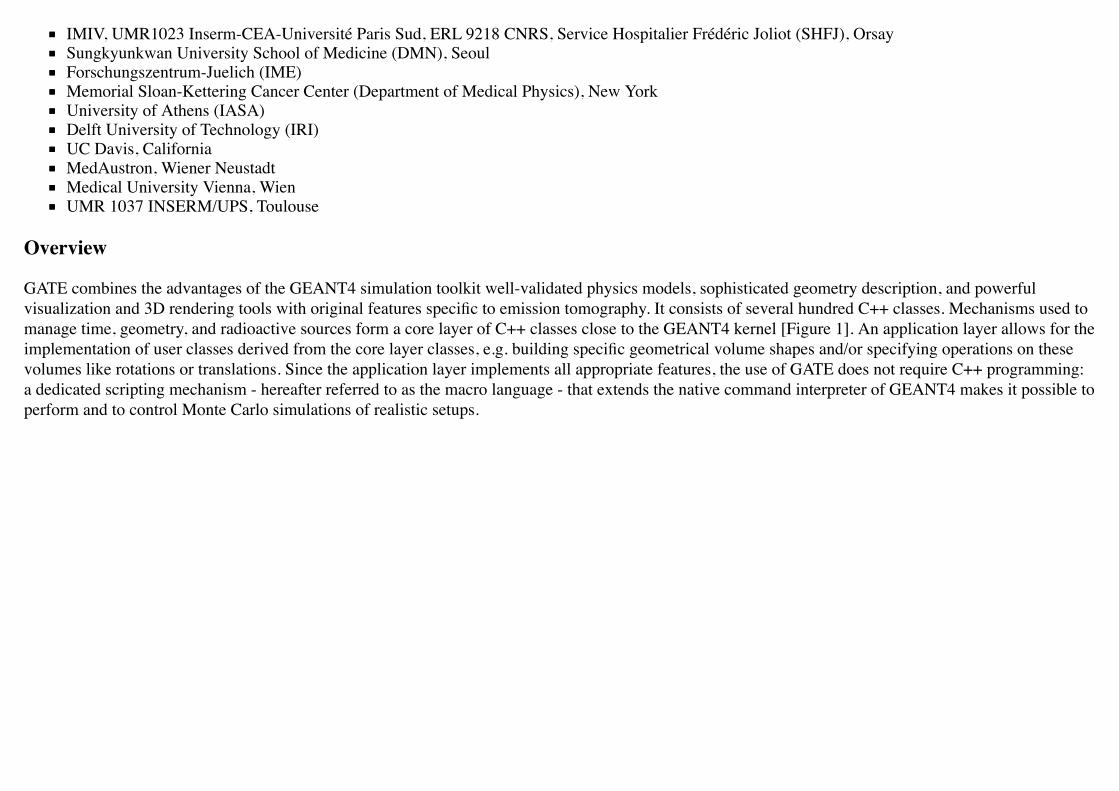
GATE combines the advantages of the GEANT4 simulation toolkit well-validated physics models, sophisticated geometry description, and powerfulvisualization and 3D rendering tools with original features specific to emission tomography. It consists of several hundred C++ classes. Mechanisms used tomanage time, geometry, and radioactive sources form a core layer of C++ classes close to the GEANT4 kernel [Figure 1]. An application layer allows for theimplementation of user classes derived from the core layer classes, e.g. building specific geometrical volume shapes and/or specifying operations on thesevolumes like rotations or translations. Since the application layer implements all appropriate features, the use of GATE does not require C++ programming:a dedicated scripting mechanism - hereafter referred to as the macro language - that extends the native command interpreter of GEANT4 makes it possible toperform and to control Monte Carlo simulations of realistic setups.

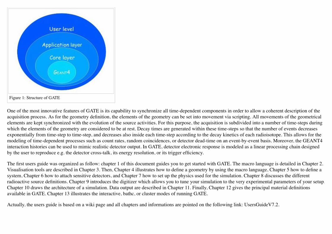
Figure 1: Structure of GATE

One of the most innovative features of GATE is its capability to synchronize all time-dependent components in order to allow a coherent description of theacquisition process. As for the geometry definition, the elements of the geometry can be set into movement via scripting. All movements of the geometricalelements are kept synchronized with the evolution of the source activities. For this purpose, the acquisition is subdivided into a number of time-steps duringwhich the elements of the geometry are considered to be at rest. Decay times are generated within these time-steps so that the number of events decreasesexponentially from time-step to time-step, and decreases also inside each time-step according to the decay kinetics of each radioisotope. This allows for themodeling of time-dependent processes such as count rates, random coincidences, or detector dead-time on an event-by-event basis. Moreover, the GEANT4interaction histories can be used to mimic realistic detector output. In GATE, detector electronic response is modeled as a linear processing chain designedby the user to reproduce e.g. the detector cross-talk, its energy resolution, or its trigger efficiency.

The first users guide was organized as follow: chapter 1 of this document guides you to get started with GATE. The macro language is detailed in Chapter 2.Visualisation tools are described in Chapter 3. Then, Chapter 4 illustrates how to define a geometry by using the macro language, Chapter 5 how to define asystem, Chapter 6 how to attach sensitive detectors, and Chapter 7 how to set up the physics used for the simulation. Chapter 8 discusses the differentradioactive source definitions. Chapter 9 introduces the digitizer which allows you to tune your simulation to the very experimental parameters of your setup.Chapter 10 draws the architecture of a simulation. Data output are described in Chapter 11. Finally, Chapter 12 gives the principal material definitionsavailable in GATE. Chapter 13 illustrates the interactive, bathc, or cluster modes of running GATE.

Actually, the users guide is based on a wiki page and all chapters and informations are pointed on the following link: UsersGuideV7.2.

Retrieved from "http://wiki.opengatecollaboration.org/index.php?title=UsersGuideV8.0:Introduction&oldid=249"

This page was last modified on 4 July 2016, at 14:40.

Users Guide V8.0:Getting startedFrom Wiki OpenGATE

This paragraph is an overview of the main steps one must go through to perform a simulation using Gate. It is presented in the form of a simple example thatthe user is encouraged to try out, while reading this section. A more detailed description of the different steps is given in the following sections of this user'sguide. The use of Gate does not require any C++ programming, thanks to a dedicated scripting mechanism that extends the native command interpreter ofGeant4. This interface allows the user to run Gate programs using command scripts only. The goal of this first section is to give a brief description of theuser interface and to provide understanding of the basic principles of Gate by going through the different steps of a simulation.

Contents1 Simulation architecture for imaging applications2 Simulation architecture for dosimetry and radiotherapy applications3 The user interface: a macro language4 Step 1: Defining a scanner geometry5 Second step: Defining a phantom geometry6 Third step: Setting-up the physics processes7 Fourth step: Initialization8 Fifth step: Setting-up the digitizer9 Sixth step: Setting-up the source10 Seventh step: Defining data output11 Eighth step: Starting an acquisition

11.1 Regular time slice approach11.2 Slices with variable time

12 Verbosity

Simulation architecture for imaging applicationsIn each simulation, the user has to:

1. define the scanner geometry2. define the phantom geometry3. set up the physics processes4. initialize the simulation :

/gate/run/initialize

1. set up the detector model2. define the source(s)3. specify the data output format4. start the acquisition

Steps 1) to 4) concern the initialization of the simulation. Following the initialization, the geometry can no longer be changed.

Simulation architecture for dosimetry and radiotherapy applicationsIn each simulation, the user has to:

1. define the beam geometry2. define the phantom geometry3. specify the output (actor concept for dose map etc...)4. set up the physics processes5. initialize the simulation :

/gate/run/initialize

1. define the source(s)2. start the simulation with the following command lines:

/gate/application/setTotalNumberOfPrimaries [particle_number]

/gate/application/start

The user interface: a macro language

Gate, just as GEANT4, is a program in which the user interface is based on scripts. To perform actions, the user must either enter commands in interactivemode, or build up macro files containing an ordered collection of commands.

Each command performs a particular function, and may require one or more parameters. The Gate commands are organized following a tree structure, withrespect to the function they represent. For example, all geometry-control commands start with geometry, and they will all be found under the /geometry/branch of the tree structure.

When Gate is run, the Idle> prompt appears. At this stage the command interpreter is active; i.e. all the Gate commands entered will be interpreted andprocessed on-line. All functions in Gate can be accessed to using command lines. The geometry of the system, the description of the radioactive source(s),the physical interactions considered, etc., can be parameterized using command lines, which are translated to the Gate kernel by the command interpreter. Inthis way, the simulation is defined one step at a time, and the actual construction of the geometry and definition of the simulation can be seen on-line. If theeffect is not as expected, the user can decide to re-adjust the desired parameter by re-entering the appropriate command on-line. Although enteringcommands step by step can be useful when the user is experimenting with the software or when he/she is not sure how to construct the geometry, thereremains a need for storing the set of commands that led to a successful simulation.

Macros are ASCII files (with '.mac' extension) in which each line contains a command or a comment. Commands are GEANT4 or Gate scripted commands;comments start with the character ' #'. Macros can be executed from within the command interpreter in Gate, or by passing it as a command-line parameterto Gate, or by calling it from another macro. A macro or set of macros must include all commands describing the different components of a simulation in theright order. Usually these components are visualization, definitions of volumes (geometry), systems, digitizer, physics, initialization, source, output and start.These steps are described in the next sections. A single simulation may be split into several macros, for instance one for the geometry, one for the physics,etc. Usually, there is a master macro which calls the more specific macros. Splitting macros allows the user to re-use one or more of these macros in severalother simulations, and/or to organize the set of all commands. Examples of complete macros can be found on the web site referenced above. To execute amacro (mymacro.mac in this example) from the Linux prompt, just type :

Gate mymacro.mac

To execute a macro from inside the Gate environment, type after the "Idle>" prompt:

Idle>/control/execute mymacro.mac

And finally, to execute a macro from inside another macro, simply write in the master macro:

/control/execute mymacro.mac

Fig 1.1: World volume.

In the following sections, the main steps to perform a simulation for imaging applications using Gate are presented in details. To try out this example, theuser can run Gate and execute all the proposed commands, line by line.

Step 1: Defining a scanner geometryThe user needs to define the geometry of the simulation based on volumes. All volumes are linkedtogether following a tree structure where each branch represents a volume. Each volume is characterizedby shape, size, position, and material composition. The default material assigned to a new volume is Air.The list of available materials is defined in the GateMaterials.db file. (See Users Guide V8.0:Materials).The location of the material database needs to be specified with the following command:

/gate/geometry/setMaterialDatabase MyMaterialDatabase.db

The base of the tree is represented by the world volume (fig 1.1) which sets the experimental frameworkof the simulation. All Gate commands related to the construction of the geometry are described in detail inUsers Guide V8.0:Defining a geometry. The world volume is a box centered at the origin. It can be of anysize and has to be large enough to include the entire simulation geometry. The tracking of any particlestops when it escapes from the world volume. The example given here simulates a system that fits into abox of 40 x 40 x 40 cm3. Thus, the world volume may be defined as follows:

# W O R L D/gate/world/geometry/setXLength 40. cm /gate/world/geometry/setYLength 40. cm /gate/world/geometry/setZLength 40. cm

The world contains one or more sub volumes referred to as daughter volumes.

/gate/world/daughters/name vol_name

The name vol_name of the first daughter of the world has a specific meaning and name. It specifies the type of scanner to be simulated. Users GuideV8.0:Defining a system gives the specifics of each type of scanner, also called system. In the current example, the system is a CylindricalPET system. Thissystem assumes that the scanner is based on a cylindrical configuration (fig 1.2) of blocks, each block containing a set of crystals.

Figure 1.2: Cylindrical scanner

# S Y S T E M/gate/world/daughters/name cylindricalPET/gate/world/daughters/insert cylinder/gate/cylindricalPET/setMaterial Water/gate/cylindricalPET/geometry/setRmax 100 mm/gate/cylindricalPET/geometry/setRmin 86 mm/gate/cylindricalPET/geometry/setHeight 18 mm/gate/cylindricalPET/vis/forceWireframe/vis/viewer/zoom 3

These seven command lines describe the global geometry of the scanner. The shape of the scanner is acylinder filled with water with an external radius of 100 mm and an internal radius of 86 mm. The lengthof the cylinder is 18 mm. The last command line sets the visualization as wireframe.

You may see the following message when creating the geometry:

G4PhysicalVolumeModel::Validate() called.Volume of the same name and copy number ("world_phys", copy 0) still exists and is being used.WARNING: This does not necessarily guarantee it's the samevolume you originally specified in /vis/scene/add/.

This message is normal and you can safely ignore it.

At any time, the user can list all the possible commands. For example, the command line for listing the visualization commands is:

Idle> ls /gate/cylindricalPET/vis/

Let's assume that the scanner is made of 30 blocks (box1), each block containing textstyle 8 times 8 LSO crystals (box2).

The following command lines describe this scanner (see Users Guide V8.0:Defining a geometry to find a detailed explanation of these commands). First, thegeometry of each block needs to be defined as the daughter of the system (here cylindricalPET system).

# FIRST LEVEL OF THE SYSTEM/gate/cylindricalPET/daughters/name box1/gate/cylindricalPET/daughters/insert box/gate/box1/placement/setTranslation 91. 0 0 mm/gate/box1/geometry/setXLength 10. mm/gate/box1/geometry/setYLength 17.75 mm

Figure 1.3: first level of the scanner

/gate/box1/geometry/setZLength 17.75 mm/gate/box1/setMaterial Water/gate/box1/vis/setColor yellow/gate/box1/vis/forceWireframe

Once the block is created (fig 1.3), the crystal can be defined as a daughter of the block (fig 1.4)

The zoom command line in the script allows the user to zoom the geometry and the panTo commandtranslates the viewer window in 60 mm in horizontal and 40 mm in vertical directions (the default is theorigin of the world (0,0,0)).

To obtain the complete matrix of crystals, the volume box2 needs to be repeated in the Y and Z directions(fig 1.5). To obtain the complete ring detector, the original block is repeated 30 times (fig 1.6).

# C R Y S T A L/gate/box1/daughters/name box2/gate/box1/daughters/insert box/gate/box2/geometry/setXLength 10. mm/gate/box2/geometry/setYLength 2. mm/gate/box2/geometry/setZLength 2. mm/gate/box2/setMaterial LSO/gate/box2/vis/setColor red/gate/box2/vis/forceWireframe

# Z O O M/vis/viewer/zoom 4/vis/viewer/panTo 60 -40 mm

# R E P E A T C R Y S T A L/gate/box2/repeaters/insert cubicArray/gate/box2/cubicArray/setRepeatNumberX 1/gate/box2/cubicArray/setRepeatNumberY 8/gate/box2/cubicArray/setRepeatNumberZ 8/gate/box2/cubicArray/setRepeatVector 0. 2.25 2.25 mm

The geometry of this simple PET scanner has now been specified. The next step is to connect this geometry to the system in order to store data from particleinteractions (called hits) within the volumes which represent detectors (sensitive detector or physical volume). Gate only stores hits for those volumesattached to a sensitive detector. Hits regarding interactions occurring in non-sensitive volumes are lost. A volume must belong to a system before it can be

Figure 1.4: crystal, daughter of the block

attached to a sensitive detector. Hits, occurring in a volume, cannot be scored in an output file if this volume is not connected to a system because thisvolume can not be attached to a sensitive detector. The concepts of system and sensitive detector are discussed in more detail in Users Guide V8.0:Defininga system and Users Guide V8.0:Attaching the sensitive detectors respectively.

The following commands are used to connect the volumes to the system.

# R E P E A T R S E C T O R /gate/box1/repeaters/insert ring/gate/box1/ring/setRepeatNumber 30

# Z O O M/vis/viewer/zoom 0.25/vis/viewer/panTo 0 0 mm

# A T T A C H V O L U M E S T O A S Y S T E M /gate/systems/cylindricalPET/rsector/attach box1 /gate/systems/cylindricalPET/module/attach box2

The names rsector and module are dedicated names and correspond to the first and the second levels of theCylindricalPET system (see Users Guide V8.0:Defining a system).

In order to save the hits (see Users Guide V8.0:Digitizer and readout parameters) in the volumescorresponding to the crystals the appropriate command, in this example, is:

# D E F I N E A S E N S I T I V E D E T E C T O R/gate/box2/attachCrystalSD vglue 1cm

At this level of the macro file, the user can implement detector movement. One of the most distinctivefeatures of Gate is the management of time-dependent phenomena, such as detector movements and sourcedecay leading to a coherent description of the acquisition process. For simplicity, the simulation described inthis tutorial does not take into account the motion of the detector or the phantom. Users GuideV8.0:Defining a geometry describes the movement of volumes in detail.

Second step: Defining a phantom geometry

Figure 1.5: matrix of crystals

The volume to be scanned is built according to the same principle used to build the scanner. The external envelope of the phantom is a daughter of the world.The following command lines describe a cylinder with a radius of 10 mm and a length of 30 mm. The cylinder is filled with water and will be displayed ingray. This object represents the attenuation medium of the phantom.

# P H A N T O M/gate/world/daughters/name my_phantom/gate/world/daughters/insert cylinder/gate/my_phantom/setMaterial Water/gate/my_phantom/vis/setColor grey/gate/my_phantom/geometry/setRmax 10. mm/gate/my_phantom/geometry/setHeight 30. mm

To retrieve information about the Compton and the Rayleigh interactions within the phantom, a sensitivedetector (phantomSD) is associated with the volume using the following command line:

# P H A N T O M D E F I N E D A S S E N S I T I V E /gate/my_phantom/attachPhantomSD

Two types of information will now be recorded for each hit in the hit collection:

The number of scattering interactions generated in all physical volumes attached to the phantomSD.The name of the physical volume attached to the phantomSD in which the last interaction occurred.

These concepts are further discussed in Users Guide V8.0:Attaching the sensitive detectors.

Third step: Setting-up the physics processesOnce the volumes and corresponding sensitive detectors are described, the interaction processes of interest in the simulation have to be specified. Gate usesthe GEANT4 models for physical processes. The user has to choose among these processes for each particle. Then, user can customize the simulation bysetting the production thresholds, the cuts, the electromagnetic options...

Some typical physics lists are available in the directory examples/PhysicsLists:

egammaStandardPhys.mac (physics list for photons, e- and e+ with standard processes and recommended Geant4 "option3")egammaLowEPhys.mac (physics list for photons, e- and e+ with low energy processes)egammaStandardPhysWithSplitting.mac (alternative egammaStandardPhys.mac with selective bremsstrahlung splitting)

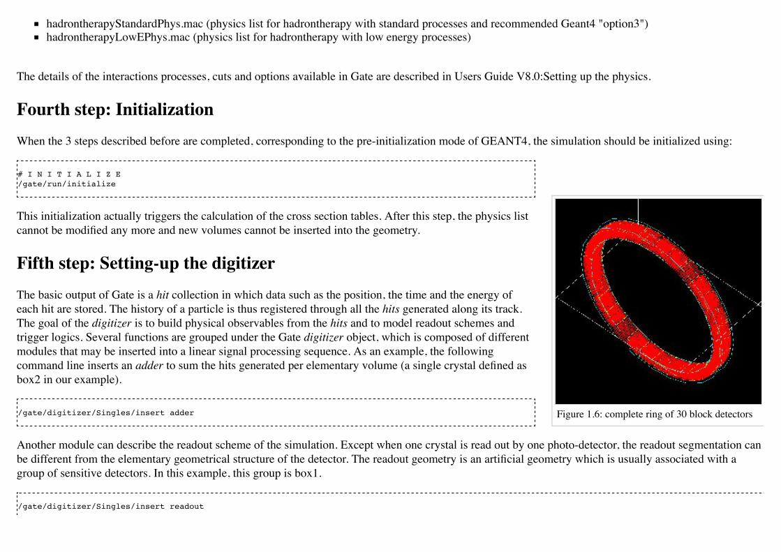
Figure 1.6: complete ring of 30 block detectors

hadrontherapyStandardPhys.mac (physics list for hadrontherapy with standard processes and recommended Geant4 "option3")hadrontherapyLowEPhys.mac (physics list for hadrontherapy with low energy processes)

The details of the interactions processes, cuts and options available in Gate are described in Users Guide V8.0:Setting up the physics.

Fourth step: InitializationWhen the 3 steps described before are completed, corresponding to the pre-initialization mode of GEANT4, the simulation should be initialized using:

# I N I T I A L I Z E /gate/run/initialize

This initialization actually triggers the calculation of the cross section tables. After this step, the physics listcannot be modified any more and new volumes cannot be inserted into the geometry.

Fifth step: Setting-up the digitizerThe basic output of Gate is a hit collection in which data such as the position, the time and the energy ofeach hit are stored. The history of a particle is thus registered through all the hits generated along its track.The goal of the digitizer is to build physical observables from the hits and to model readout schemes andtrigger logics. Several functions are grouped under the Gate digitizer object, which is composed of differentmodules that may be inserted into a linear signal processing sequence. As an example, the followingcommand line inserts an adder to sum the hits generated per elementary volume (a single crystal defined asbox2 in our example).

/gate/digitizer/Singles/insert adder

Another module can describe the readout scheme of the simulation. Except when one crystal is read out by one photo-detector, the readout segmentation canbe different from the elementary geometrical structure of the detector. The readout geometry is an artificial geometry which is usually associated with agroup of sensitive detectors. In this example, this group is box1.

/gate/digitizer/Singles/insert readout

Figure 1.7: cylindrical phantom

/gate/digitizer/Singles/readout/setDepth 1

In this example, the readout module sums the energy deposited in all crystals within the block and determines the position of the crystal with the highestenergy deposited ("winner takes all"). The setDepth command specifies at which geometry level (called "depth") the readout function is performed. In thecurrent example:

base level (CylindricalPET) = depth 01srt daughter (box1) of the system = depth 1next daughter (box2) of the system = depth 2and so on ....

In order to take into account the energy resolution of the detector and to collect singles within a pre-definedenergy window only, other modules can be used:

# E N E R G Y B L U R R I N G/gate/digitizer/Singles/insert blurring/gate/digitizer/Singles/blurring/setResolution 0.19/gate/digitizer/Singles/blurring/setEnergyOfReference 511. keV

# E N E R G Y W I N D O W/gate/digitizer/Singles/insert thresholder/gate/digitizer/Singles/thresholder/setThreshold 350. keV/gate/digitizer/Singles/insert upholder/gate/digitizer/Singles/upholder/setUphold 650. keV

Here, an energy resolution of 19% at 551 KeV is considered.

Furthermore, the energy window is set from 350 keV to 600 keV.

For PET simulations, the coincidence sorter is also implemented at the digitizer level.

# C O I N C I D E N C E S O R T E R/gate/digitizer/Coincidences/setWindow 10. ns

Other digitizer modules are available in Gate and are described in Users Guide V8.0:Digitizer and readout parameters.

Sixth step: Setting-up the source

In Gate, a source is represented by a volume in which the particles (positron, gamma, ion, proton, ...) are emitted. The user can define the geometry of thesource and its characteristics such as the direction of emission, the energy distribution, and the activity. The lifetime of unstable sources (radioactive ions) isusually obtained from the GEANT4 database, but it can also be set by the user.

A voxelized phantom or a patient dataset can also be used to define the source, in order to simulate realistic acquisitions. For a complete description of allfunctions to define the sources, see Users Guide V8.0:Voxelized Source and Phantom.

In the current example, the source is a 1 MBq line source. The line source is defined as a cylinder with a radius of 0.5 mm and a length of 50 mm. Thesource generates pairs of 511 keV gamma particles emitted 'back-to-back' (for a more realistic source model, the range of the positron and the noncollinearity of the two gammas can also be taken into account).

# S O U R C E/gate/source/addSource twogamma/gate/source/twogamma/setActivity 100000. becquerel/gate/source/twogamma/setType backtoback

# POSITION/gate/source/twogamma/gps/centre 0. 0. 0. cm

# PARTICLE/gate/source/twogamma/gps/particle gamma/gate/source/twogamma/gps/energytype Mono/gate/source/twogamma/gps/monoenergy 0.511 MeV

# TYPE = Volume or Surface/gate/source/twogamma/gps/type Volume

# SHAPE = Sphere or Cylinder/gate/source/twogamma/gps/shape Cylinder/gate/source/twogamma/gps/radius 0.5 mm/gate/source/twogamma/gps/halfz 25 mm

# SET THE ANGULAR DISTRIBUTION OF EMISSION/gate/source/twogamma/gps/angtype iso

# SET MIN AND MAX EMISSION ANGLES/gate/source/twogamma/gps/mintheta 0. deg/gate/source/twogamma/gps/maxtheta 180. deg/gate/source/twogamma/gps/minphi 0. deg/gate/source/twogamma/gps/maxphi 360. deg/gate/source/list

Seventh step: Defining data outputBy default, the data output formats for all systems used by Gate are ASCII and ROOT as described in the following command lines:

# ASCII OUTPUT FORMAT/gate/output/ascii/enable/gate/output/ascii/setFileName test/gate/output/ascii/setOutFileHitsFlag 0/gate/output/ascii/setOutFileSinglesFlag 1/gate/output/ascii/setOutFileCoincidencesFlag 1# ROOT OUTPUT FORMAT/gate/output/root/enable/gate/output/root/setFileName test/gate/output/root/setRootSinglesFlag 1/gate/output/root/setRootCoincidencesFlag 1

Given this script, several ASCII files (.dat extension) and A ROOT file (test.root) will be created. Users Guide V8.0:Data output explains how to read theresulting files.

For some scanner configurations, the events may be stored in a sinogram format or in List Mode Format (LMF). The sinogram output module stores thecoincident events from a cylindrical scanner system in a set of 2D sinograms according to the parameters set by the user (number of radial bins and angularpositions). One 2D sinogram is created for each pair of crystal-rings. The sinograms are stored either in raw format or ecat7 format. The List Mode Format isthe format developed by the Crystal Clear Collaboration (LGPL licence). A library has been incorporated in Gate to read, write, and analyze the LMFformat. A complete description of all available outputs is given in Users Guide V8.0:Data output .

Eighth step: Starting an acquisitionIn the next and final step the acquisition is defined. The beginning and the end of the acquisition are defined as in a real life experiment. In addition, Gateneeds a time slice parameter which defines time period during which the simulated system is assumed to be static. At the beginning of each time-slice, thegeometry is updated according to the requested movements. During each time-slice, the geometry is kept static and the simulation of particle transport anddata acquisition proceeds. Each slice corresponds to a Geant4 run.

If the sources involved in the simulation are not radioactive or if activity is not defined, user can fix the total number of events. In this case, the number ofparticles is splitted between slices in function of the time of each slice.

/gate/application/setTotalNumberOfPrimaries [N]

User can also fix the same number of events per slice. In this case, each event is weighted by the ratio between the time slice and the total simulation time.

/gate/application/setNumberOfPrimariesPerRun [N]

Regular time slice approach

This is the standard Gate approach for imaging applications (PET, SPECT and CT). User has to define the beginning and the end of the acquisition using thecommands setTimeStart and setTimeStop. Each slice has the same duration. User has to define the slice duration (setTimeSlice).

/gate/application/setTimeSlice 1. s/gate/application/setTimeStart 0. s/gate/application/setTimeStop 1. s

The choice of the generator seed is also extremely important. There are 3 ways to make that choice:

The ’default’ option. In this case the default CLHEP internal seed is taken. This seed is always

the same.

The ’auto’ option. In this case, a new seed is automatically generated each time GATE is run.

To randomly generate the seed, the time in millisecond since January 1, 1970 and the process ID of the GATE instance (i.e. the system ID of the runningGATE process) are used. So each time GATE is run, a new seed is used.

The ’manual’ option. In this case, the user can manually set the seed. The seed is an unsigned integer value and it is recommended to be included inthe interval [0,900000000].

The commands associated to the choice of the seed with the 3 different options are the following:

/gate/random/setEngineSeed default/gate/random/setEngineSeed auto/gate/random/setEngineSeed 123456789

It is also possible to control directly the initialization of the engine by selecting the file containing the seeds with the command:

/gate/random/resetEngineFrom fileName

# S T A R T the A C Q U I S I T I O N/gate/application/startDAQ

The number of projections or runs of the simulation is thus defined by:

Figure 1.8: Simulation is started

In the current example, there is no motion, the acquisition time equals 1 second and the number of projections equals one.

If you want to exit from the Gate program when the simulation time exceed the time duration, the last line of your program has to be exit.

As a Monte Carlo tool, GATE needs a random generator. The CLHEP libraries provide various ones. Three different random engines are currently availablein GATE, the Ranlux64, the James Random and the Mersenne Twister. The default one is the Mersenne Twister, but this can be changed easily using:

/gate/random/setEngineName aName (where aName can be: Ranlux64, JamesRandom, or MersenneTwister)

NB Several users have reported artifacts in PET data when using the Ranlux64 generator. These users have said that the artifacts are not present in datagenerated with the Mersenne Twister generator.

Slices with variable time

In this approach, each slice has a specific duration. User has to defined the time of each slice. The first method is to use a file of time slices:

/gate/application/readTimeSlicesIn [File Name]

the second method is to add each slice with the command:

/gate/application/addSlice [value] [unit]

User has to define the beginning of the acquisition using the command setTimeStart. The end of acquisition is calculated by summing each time slice. Thesimulation is started with the commands:

/gate/application/start

or

/gate/application/startDAQ

VerbosityThe level of verbosity of the random engine can be chosen. It consists into printing the random engine status, depending on the type of generator used. Thecommand associated to the verbosity is:

/gate/random/verbose 1

Values from 0 to 2 are allowed, higher values will be interpreted as 2. A value of 0 means no printing at all, a value of 1 results in one printing at thebeginning of the acquisition, and a value of 2 results in one printing at each beginning of run.

Figure 1.9: GATE simulation architecture

Retrieved from "http://wiki.opengatecollaboration.org/index.php?title=Users_Guide_V8.0:Getting_started&oldid=912"


Users Guide V8.0:Defining a geometryFrom Wiki OpenGATE

The definition of a geometry is a key step in designing a simulation because it is through the geometry definition that the imaging device and object to bescanned are described. Particles are then tracked through the components of the geometry. This section explains how to define the different components ofthe geometry.

Contents1 The world

1.1 Definition1.2 Use1.3 Description and modification

2 Creating a volume2.1 Generality - Tree creation2.2 Units2.3 Axes2.4 Building a volume

2.4.1 Examples2.4.1.1 How to build a NaI crystal2.4.1.2 How to build a "trpd" volume2.4.1.3 How to build a "wedge" volume2.4.1.4 How to build a "tessellated" volume

3 Repeating a volume3.1 Linear repeater3.2 Ring repeater3.3 Cubic array repeater3.4 Quadrant repeater3.5 Sphere repeater

3.6 Generic repeater4 Placing a volume

4.1 Translation4.2 Rotation4.3 Alignment4.4 Special example: Wedge volume and OPET scanner

5 Moving a volume5.1 Translation5.2 Rotation5.3 Orbiting5.4 Wobbling5.5 Eccentric rotation5.6 Generic move5.7 Generic repeater move

6 Updating the geometry

The world

Definition

The world is the only volume already defined in GATE when starting a macro. All volumes are defined as daughters or grand-daughters of the world. Theworld volume is a typical example of a GATE volume and has predefined properties. The world volume is a box centered at the origin. For any particle,tracking stops when it escapes from the world volume. The world volume can be of any size and has to be large enough to include all volumes involved inthe simulation.

Use

The first volume that can be created must be the daughter of the world volume. Any volume must be included in the world volume. The geometry is builtfrom the world volume.

Description and modification

The world volume has default parameters: shape, dimensions, material, visibility attributes and number of children. These parameters can be edited using thefollowing GATE command:

/gate/world/describe

The output of this command is shown in figure 3.1. The parameters associated with the world volume can be modified to be adapted to a specific simulationconfiguration. Only the shape of the world volume, which is a box, cannot be changed. For instance, the X length can be changed from 50 cm to 2 m using:

/gate/world/geometry/setXLength 2. m

Figure 3.1: Description of the default parameters associated with theworld

The other commands needed to modify the world volume attributes will be given in the next sections.

Creating a volume

Generality - Tree creation

When a volume is created with GATE, it automatically appears in the GATE tree. All commands applicable to the new volume are then available from thisGATE tree. For instance, if the name of the created volume is Volume_Name, all commands applicable to this volume start with:

/gate/Volume_Name/

The tree includes the following commands:

setMaterial: To assign a material to the volumeattachCrystalSD: To attach a crystal-SensitiveDetector to the volumeattachPhantomSD: To attach a phantom-SensitiveDetector to the volumeenable: To enable the volumedisable: To disable the volumedescribe: To describe the volume

The tree includes sub-trees that relate to different attributes of the volume Volume_Name. The available sub-trees are:

daughters: To insert a new 'daughter' in the volumegeometry: To control the geometry of the volumevis: To control the display attributes of the volumerepeaters: To apply a new 'repeater' to the volumemoves: To 'move' the volumeplacement: To control the placement of the volume

The commands available in each sub-tree will be described in #Building a volume, #Repeating a volume, #Placing a volume, #Moving a volume.

Units

Different units are predefined in GATE (see Table 3.1) and shall be referred to using the corresponding abbreviation. Inside the GATE environment, the listof units available in GATE can be edited using:

/units/list

Axes

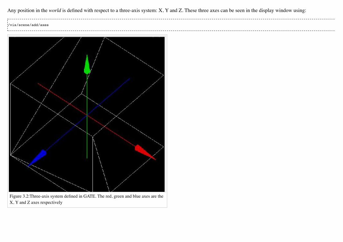
Any position in the world is defined with respect to a three-axis system: X, Y and Z. These three axes can be seen in the display window using:

/vis/scene/add/axes

Figure 3.2:Three-axis system defined in GATE. The red, green and blue axes are theX, Y and Z axes respectively

List of units available in GATE and corresponding abbreviationsLENGTH SURFACE VOLUME ANGLE

parsec pc radian radkilometer km kilometer2 km2 kilometer3 km3 milliradian mrad

meter m meter2 m2 meter33 m3 steradian sr

centimeter cm centimeter2 cm2 centimeter3 cm3 degre deg

millimeter mm millimeter2 mm2 millimeter3 mm3

micrometer mumnanometer nmangstrom Ang

TIME SPEED ANGULAR SPEED ENERGYsecond s meter/s m/s radian/s rad/s electronvolt eVmillisecond ms centimeter/s cm/s degree/s deg/s kiloelectronvolt KeVmicrosecond mus millimeter/s mm/s megaelectronvolt MeVnanosecond ns meter/min m/min radian/min rad/min gigaelectronvolt GeVpicosecond ps centimeter/min cm/min degree/s deg/s teraelectronvolt TeV

millimeter/min m/min rotation/s rot/s petaelectronvolt PeVmeter/h m/h degree/min deg/min joule jcentimer/h cm/h degree/min deg/minmillimeter/h mm/h rotation/min rot/minrotation/h rot/h radian/h rad/h

degree/h deg/hACTIVITY DOSE AMOUNT OF SUBSTANCE MASS VOLUMIC MASS

becquerel Bq mole mol milligram mg g/cm3 g/cm3

curie Ci mg/cm3 mg/cm3gray Gy kilogram kg kg/m3 kg/m3ELECTRIC CHARGE ELECTRIC CURRENT ELECTRIC POTENTIAL MAGNETIC FLUX - MAGNETIC FLUX DENSITYeplus e+ ampere A volt V weber Wbcoulomb C milliamper mA kilovolt kV tesla Tmicroampere muA megavolt MV gauss Gnanoampere nA kilogauss kG

TEMPERATURE FORCE - PRESSURE POWER FREQUENCYkelvin K newton N watt W hertz Hz

pascal Pa kilohertz kHzbar bar megaherz MHzatmosphere atm

Building a volume

Any new volume must be created as the daughter of another volume (i.e., World volume or another volume previously created).

Three rules must be respected when creating a new volume:

A volume which is located inside another must be its daughterA daughter must be fully included in its motherVolumes must not overlap

Errors in building the geometry yield wrong particle transportation, hence misleading results!

Creating a new volume

To create a new volume, the first step is to give it a name and a mother using:

/gate/mother_Volume_Name/daughters/name Volume_Name

This command prepares the creation of a new volume named Volume_Name which is the daughter of mother_Volume_Name.

Some names should not be used as they have precise meanings in gate. These names are the names of the GATE systems (see Users Guide V8.0:Defining asystem) currently defined in GATE: scanner, PETscanner, cylindricalPET, SPECTHead, ecat, CPET, OPET and OpticalSystem.

The creation of a new volume is completed only when assigning a shape to the new volume. The tree

/gate/Volume_Name/

is then generated and all commands in the tree and the sub-trees are available for the new volume.

Different volume shapes are available, namely: box, sphere, cylinder, cone, hexagon, general or extruded trapezoid, wedge, elliptical tube andtessellated.

The command line for listing the available shapes is:

/gate/world/daughters/info

The command line for assigning a shape to a volume is:

/gate/mother_Volume_Name/daughters/insert Volume_shape

where Volume_shape is the shape of the new volume.

Volume_shape must necessarily be one of the available names:

box for a box - sphere for a sphere - cylinder for a cylinder - ellipsoid for an ellipsoid - cone for a cone - eltub for a tube with an elliptical base - hexagonefor an hexagon - polycone for a polygon - trap for a general trapezoid - trpd for an extruded trapezoid - wedge for a wedge and tessellated for a tessellatedvolume.

The command line assigns the shape to the last volume that has been named.

The following command lists the daughters of a volume:

/gate/Volume_Name/daughters/list

Example

/gate/world/daughters/name Phantom /gate/world/daughters/insert box

The new volume Phantom with a box shape is inserted in the World volume.

Defining a size

After creating a volume with a shape, its dimensions are the default dimensions associated with that shape. These default dimensions can be modified usingthe sub-tree /geometry/

The commands available in the sub-tree depend on the shape. The different commands for each type of shape are listed in table 3.2

These commands can be found in the directory

/gate/Volume_Name/geometry (Some volumes visualisation are available here: http://gphysics.net/geant4/geant4-gdml-format.html)

BOX TRPDsetXLength: Set the length of the box along the X axis setX1Length: Set half length along X of the plane at -dz positionsetYLength: Set the length of the box along the Y axis setY1Length: Set half length along Y of the plane at -dz positionsetZLength: Set the length of the box along the Z axis setX2Length: Set half length along X of the plane at +dz positionSPHERE setY2Length: Set half length along Y of the plane at +dz positionsetRmin: Set the internal radius of the sphere (0 for full sphere) setZLength: Set half length along Z of the trapezoidsetRmax: Set the external radius of the sphere setXBoxLength: Set half length along X of the extruded boxsetPhiStart: Set the start phi angle setYBoxLength: Set half length along Y of the extruded boxsetDeltaPhi: Set the phi angular span (2PI for full sphere) setZBoxLength: Set half length along Z of the extruded boxsetThetaStart: Set the start theta angle setXBoxPos: Set center position X of the box

Commands of the sub-tree geometry for different shapes

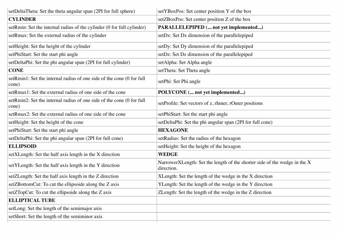
setDeltaTheta: Set the theta angular span (2PI for full sphere) setYBoxPos: Set center position Y of the boxCYLINDER setZBoxPos: Set center position Z of the boxsetRmin: Set the internal radius of the cylinder (0 for full cylinder) PARALLELEPIPED (... not yet implemented...)setRmax: Set the external radius of the cylinder setDx: Set Dx dimension of the parallelepiped

setHeight: Set the height of the cylinder setDy: Set Dy dimension of the parallelepipedsetPhiStart: Set the start phi angle setDz: Set Dz dimension of the parallelepipedsetDeltaPhi: Set the phi angular span (2PI for full cylinder) setAlpha: Set Alpha angleCONE setTheta: Set Theta anglesetRmin1: Set the internal radius of one side of the cone (0 for fullcone) setPhi: Set Phi angle

setRmax1: Set the external radius of one side of the cone POLYCONE (... not yet implemented...)setRmin2: Set the internal radius of one side of the cone (0 for fullcone) setProfile: Set vectors of z, rInner, rOuter positions

setRmax2: Set the external radius of one side of the cone setPhiStart: Set the start phi anglesetHeight: Set the height of the cone setDeltaPhi: Set the phi angular span (2PI for full cone)setPhiStart: Set the start phi angle HEXAGONEsetDeltaPhi: Set the phi angular span (2PI for full cone) setRadius: Set the radius of the hexagonELLIPSOID setHeight: Set the height of the hexagonsetXLength: Set the half axis length in the X direction WEDGE

setYLength: Set the half axis length in the Y direction NarrowerXLength: Set the length of the shorter side of the wedge in the Xdirection.

setZLength: Set the half axis length in the Z direction XLength: Set the length of the wedge in the X directionsetZBottomCut: To cut the ellipsoide along the Z axis YLength: Set the length of the wedge in the Y directionsetZTopCut: To cut the ellipsoide along the Z axis ZLength: Set the length of the wedge in the Z directionELLIPTICAL TUBEsetLong: Set the length of the semimajor axissetShort: Set the length of the semiminor axis

setHeight: Set the height of the tubeTESSELLATEDsetPathToVerticesFile: Set the path to vertices text file

For a box volume called Phantom , the X, Y and Z dimensions can be defined by:

/gate/Phantom/geometry/setXLength 20. cm /gate/Phantom/geometry/setYLength 10. cm /gate/Phantom/geometry/setZLength 5. cm

The dimensions of the Phantom volume are then 20 cm, 10 cm and 5 cm along the X, Y and Z axes respectively.

Defining a material

A material must be associated with each volume. The default material assigned to a new volume is Air. The list of available materials is defined in theGateMaterials.db file. (see Users Guide V8.0:Materials).

The following command fills the volume Volume_Name with a material called Material:

/gate/Volume_Name/setMaterial Material

Example

/gate/Phantom/setMaterial Water

The Phantom volume is filled with Water.

Defining a color or an appearance

To make the geometry easy to visualize, some display options can be set using the sub-tree /vis/

The commands available in this sub-tree are: setColor, setVisible, setDaughtersInvisible, setLineStyle, setLineWidth, forceSolid and forceWireframe (seeTable 3.3)

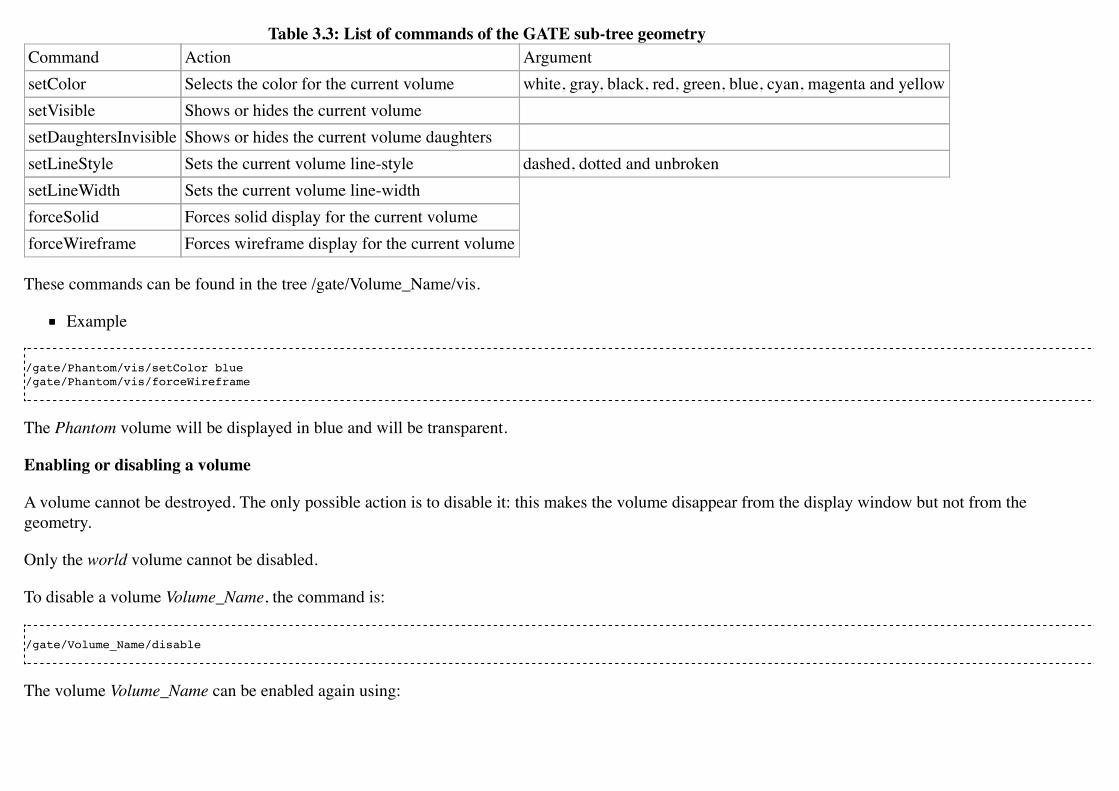
Table 3.3: List of commands of the GATE sub-tree geometryCommand Action ArgumentsetColor Selects the color for the current volume white, gray, black, red, green, blue, cyan, magenta and yellowsetVisible Shows or hides the current volumesetDaughtersInvisible Shows or hides the current volume daughterssetLineStyle Sets the current volume line-style dashed, dotted and unbrokensetLineWidth Sets the current volume line-widthforceSolid Forces solid display for the current volumeforceWireframe Forces wireframe display for the current volume

These commands can be found in the tree /gate/Volume_Name/vis.

Example

/gate/Phantom/vis/setColor blue /gate/Phantom/vis/forceWireframe

The Phantom volume will be displayed in blue and will be transparent.

Enabling or disabling a volume

A volume cannot be destroyed. The only possible action is to disable it: this makes the volume disappear from the display window but not from thegeometry.

Only the world volume cannot be disabled.

To disable a volume Volume_Name, the command is:

/gate/Volume_Name/disable

The volume Volume_Name can be enabled again using:

/gate/Volume_Name/enable

Example

/gate/Phantom/disable

The Phantom volume is disabled.

Describing a volume

The parameters associated with a volume Volume_name can be listed using:

/gate/Volume_Name/describe

Example

/gate/Phantom/describe

The parameters associated with the Phantom volume are listed.

Examples

How to build a NaI crystal

/gate/mother_Volume_Name/daughters/name crystal /gate/mother_Volume_Name/daughters/insert box

A volume named crystal is created as the daughter of a volume the shape of which is defined as a box.

/gate/crystal/geometry/setXLength 1. cm /gate/crystal/geometry/setYLength 40. cm /gate/crystal/geometry/setZLength 54. cm

The X, Y and Z dimensions of the volume crystal are set to 1 cm, 40 cm, and 54 cm respectively.

/gate/crystal/setMaterial NaI

The new volume crystal is filled with NaI.

/gate/crystal/vis/setColor yellow

The new volume crystal is colored in yellow.

/gate/crystal/describe

The previous command lists the parameters associated with the crystal volume.

/gate/crystal/disable

The crystal volume is disabled

How to build a "trpd" volume

An alternative way of describing complicated geometries is to use a so-called "boolean" volume in order to describe one piece using a single volume insteadof using a mother-children couple. This can make the description easier and more synthetic. The example below describes how the shape shown in Figure3.3 can be defined using a trpd shape, based on a "boolean" volume consisting of a trapezoid "minus" a box:

# V I S U A L I S A T I O N /vis/open OGLSX /vis/viewer/reset /vis/viewer/viewpointThetaPhi 60 60 /vis/viewer/zoom 1 /vis/viewer/set/style surface/vis/drawVolume /tracking/storeTrajectory 1 /vis/scene/endOfEventAction accumulate/vis/viewer/update/vis/verbose 2/gate/geometry/enableAutoUpdate/gate/world/daughters/name Volume_Name

Figure 3.3 Side view of an extruded trapezoid based on aboolean solid. The contours in blue and dashed redrepresent the contours of the trapezoid and the boxrespectively

/gate/world/daughters/insert box/gate/Volume_Name/geometry/setXLength 40 cm/gate/Volume_Name/geometry/setYLength 40 cm/gate/Volume_Name/geometry/setZLength 40 cm/gate/Volume_Name/vis/forceWireframe/gate/Volume_Name/daughters/name trapeze_name /gate/Volume_Name/daughters/insert trpd /gate/trapeze_name/geometry/setX1Length 23.3 mm /gate/trapeze_name/geometry/setY1Length 21.4 mm /gate/trapeze_name/geometry/setX2Length 23.3 mm /gate/trapeze_name/geometry/setY2Length 23.3 mm /gate/trapeze_name/geometry/setZLength 6. mm /gate/trapeze_name/geometry/setXBoxPos 0. mm /gate/trapeze_name/geometry/setYBoxPos 0. m /gate/trapeze_name/geometry/setZBoxPos 0.7501 mm /gate/trapeze_name/geometry/setXBoxLength 20.3 mm /gate/trapeze_name/geometry/setYBoxLength 20.3 mm /gate/trapeze_name/geometry/setZBoxLength 4.501 mm

The new volume called trapeze_name, which is the daughter of the Volume_Name volume, isdescribed with 5+6 parameters. The first 5 parameters relate to the trapezoid, whereas the last 6parameters describe the extruded volume using a box shape.

How to build a "wedge" volume

Gate provides the class GateTrapCreator to create and insert trapezoidal volumes into thegeometry. To create a trapezoid, the user needs to specify eleven parameters (besides its name andmaterial), which does not make it easy to use.

To model "slanted" crystals, a new class called GateWedgeCreator (derived from G4Trap) buildsright angular wedges. As shown in Figure 3.4, a wedge is defined by only three parameters that areeasily understood:

1. XLength: is the length of the wedge in the X direction.2. NarrowerXLength: is the length of the shorter side of the wedge in the X direction.3. YLength: is the length in the Y direction.4. ZLength: is the length in the Z direction.

For instance, the following macro lines insert a wedge crystal as a daughter of a module:

Figure 3.4: When a wedge is inserted, it is oriented as shown in this figure

/gate/module/daughters/name wedge0 /gate/module/daughters/insert wedge /gate/wedge0/geometry/setXLength 10 mm /gate/wedge0/geometry/setNarrowerXLength 8.921 mm /gate/wedge0/geometry/setYLength 2.1620 mm /gate/wedge0/geometry/setZLength 2.1620 mm /gate/wedge0/setMaterial LSO /gate/wedge0/vis/setColor yellow

How to build a "tessellated" volume

In GATE, you have the possibility to create a tessellated volume from an STLfile. STL is a common file format that uses triangular facets to define the surfaceof a three-dimensional object. This allows to simulate a complex geometryimported from a CAD software. The surface described in the STL file is used to create a volume in GATE using the Geant4 G4TessellatedSolid class. It'simportant to note that only one material is associated to a tessellated volume. You can use either ASCII or binary STL files.

Here is an example to create a tessellated volume from an STL file in a GATE macro:

/gate/world/daughters/name kidneyLeft/gate/world/daughters/insert tessellated/gate/kidneyLeft/placement/setTranslation -265.3625 -121.5875 -842.16 mm/gate/kidneyLeft/geometry/setPathToSTLFile data/Label89.stl/gate/kidneyLeft/setMaterial Kidney

Label89.stl being the STL file containing the triangular facets.

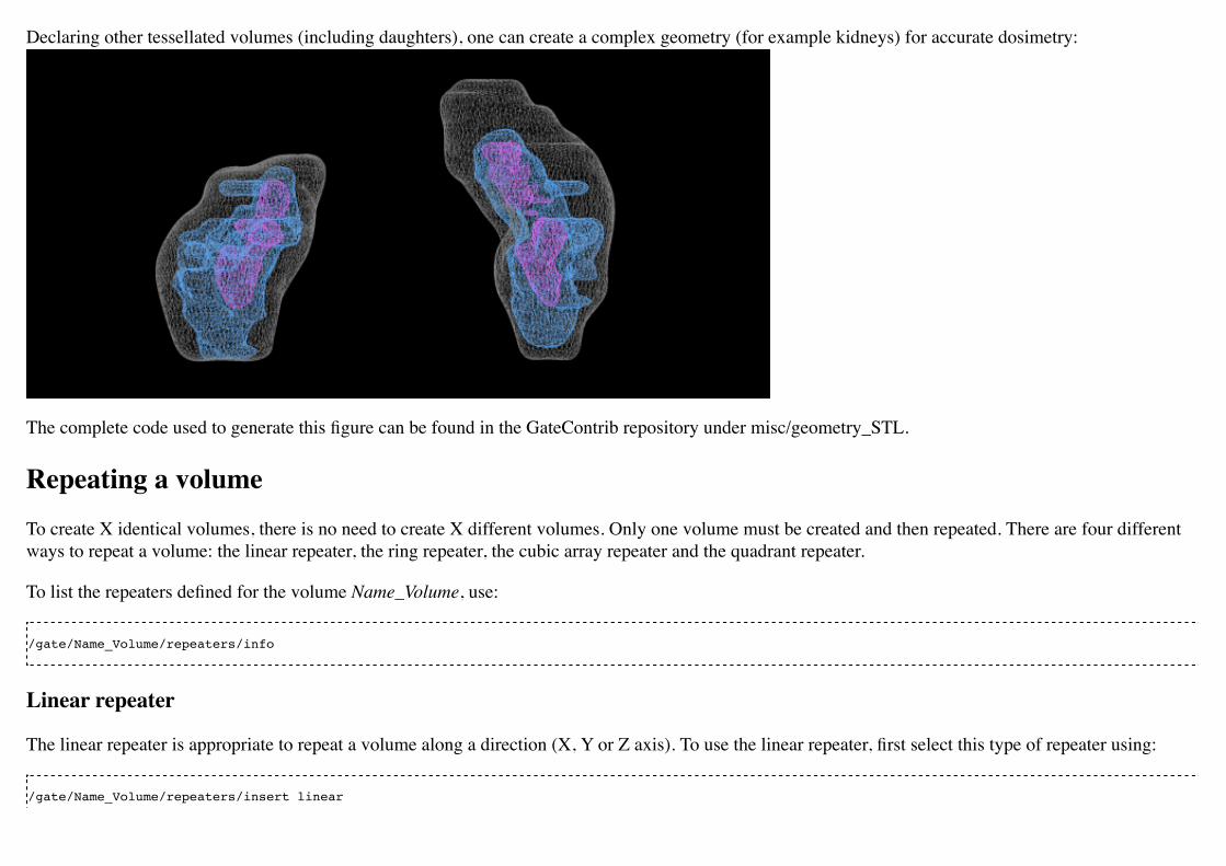
Declaring other tessellated volumes (including daughters), one can create a complex geometry (for example kidneys) for accurate dosimetry:

The complete code used to generate this figure can be found in the GateContrib repository under misc/geometry_STL.

Repeating a volumeTo create X identical volumes, there is no need to create X different volumes. Only one volume must be created and then repeated. There are four differentways to repeat a volume: the linear repeater, the ring repeater, the cubic array repeater and the quadrant repeater.

To list the repeaters defined for the volume Name_Volume, use:

/gate/Name_Volume/repeaters/info

Linear repeater

The linear repeater is appropriate to repeat a volume along a direction (X, Y or Z axis). To use the linear repeater, first select this type of repeater using:

/gate/Name_Volume/repeaters/insert linear

Then define the number of times N the volume Name_Volume has to be repeated using:

/gate/Name_Volume/linear/setRepeatNumber N

Finally, define the step and direction of the repetition using:

/gate/Name_Volume/linear/setRepeatVector 0. 0. dZ. mm

A step of dZ mm along the Z direction is defined.

The "autoCenter" command allows the user to set the position of the repeated volumes:

/gate/Name_Volume/linear/autoCenter true or false

The "true" option centers the group of repeated volumes around the position of the initial volume that has been repeated.

The "false" option centers the first copy around the position of the initial volume that has been repeated. The other copies are created by offset. The defaultoption is true.

Example

/gate/hole/repeaters/insert linear /gate/hole/linear/setRepeatNumber 12 /gate/hole/linear/setRepeatVector 0. 4. 0. cm

The hole volume is repeated 12 times every 4 cm along the Y axis. The application of this linear repeater is illustrated in figure 3.5.

Ring repeater

The ring repeater makes it possible to repeat a volume along a ring. It is useful to build a ring of detectors in PET.

To select the ring repeater, use:

/gate/Name_Volume/repeaters/insert ring

To define the number of times N the volume Name_Volume has to be repeated, use:

/gate/Name_Volume/ring/setRepeatNumber N

Finally, the axis around which the volume Name_Volume will be repeated must be defined by specifying two points using:

/gate/Name_Volume/ring/setPoint1 0. 1. 0. mm /gate/Name_Volume/ring/setPoint2 0. 0. 0. mm

The default rotation axis is the Z axis. Note that the default ring repetitiongoes counter clockwise.

These three commands are enough to repeat a volume along a ring over 360°.However, the repeat action can be further customized using one or more ofthe following commands. To set the rotation angle for the first copy, use:

/gate/Name_Volume/ring/setFirstAngle x deg

The default angle is 0 deg.

To set the rotation angle difference between the first and the last copy, use:

/gate/Name_Volume/ring/setAngularSpan x deg

The default angle is 360 deg.

The AngularSpan, the FirstAngle and the RepeatNumber allow one to definethe rotation angle difference between two adjacent copies (AngularPitch).

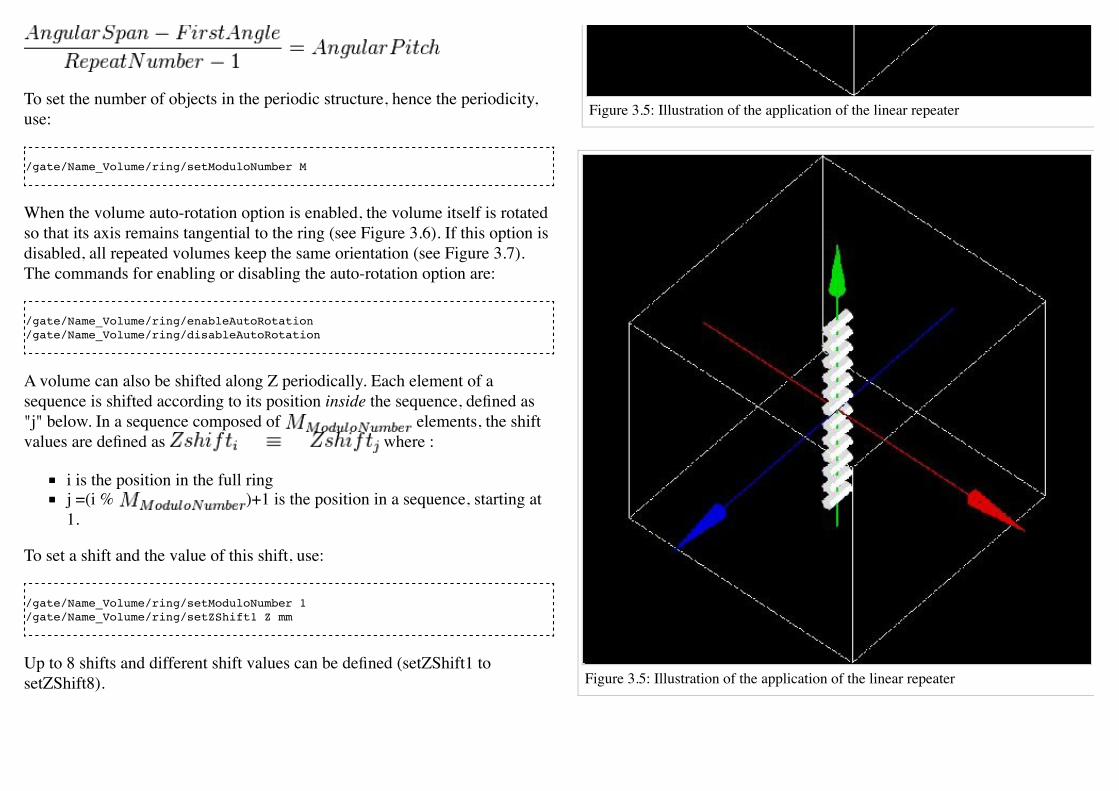
Figure 3.5: Illustration of the application of the linear repeater

Figure 3.5: Illustration of the application of the linear repeater

To set the number of objects in the periodic structure, hence the periodicity,use:

/gate/Name_Volume/ring/setModuloNumber M

When the volume auto-rotation option is enabled, the volume itself is rotatedso that its axis remains tangential to the ring (see Figure 3.6). If this option isdisabled, all repeated volumes keep the same orientation (see Figure 3.7).The commands for enabling or disabling the auto-rotation option are:

/gate/Name_Volume/ring/enableAutoRotation /gate/Name_Volume/ring/disableAutoRotation

A volume can also be shifted along Z periodically. Each element of asequence is shifted according to its position inside the sequence, defined as"j" below. In a sequence composed of elements, the shiftvalues are defined as where :

i is the position in the full ringj =(i % )+1 is the position in a sequence, starting at1.

To set a shift and the value of this shift, use:

/gate/Name_Volume/ring/setModuloNumber 1 /gate/Name_Volume/ring/setZShift1 Z mm

Up to 8 shifts and different shift values can be defined (setZShift1 tosetZShift8).

Remark: This geometry description conforms to the document "List Mode Format Implementation: Scanner geometry description Version 4.1 M.Krieguer etal " and is fully described in the LMF output, in particular in the ASCII header file entry:

z shift sector j mod : Zshift_j units

Here j (j starting here at 0) stands for the object being shifted each object. Each shift value introduced in the command line belowcorresponds to a new line in the .cch file.

The LMF version 22.10.03 supports a geometry with a cylindrical symmetry. As an example, a repeater starting at 0 degree and finishing at 90 degree (aquarter of ring) will not be supported by the LMF output.

Example 1

/gate/hole/repeaters/insert ring /gate/hole/ring/setRepeatNumber 10 /gate/hole/ring/setPoint1 0. 1. 0. mm /gate/hole/ring/setPoint2 0. 0. 0. mm

The hole volume is repeated 10 times around the Y axis. The application of this ring repeater is illustrated in figure 3.8.

Figure 3.8: Illustration of the application of the ring repeater

Figure 3.6: Illustration of the application of the auto-rotation option

Figure 3.8b: Illustration of the application of the ring repeater

Example 2

/gate/rsector/repeaters/insert ring /gate/rsector/ring/setRepeatNumber 20 /gate/rsector/ring/setModuloNumber 2 /gate/rsector/ring/setZShift1 -3500 mum /gate/rsector/ring/setZShift2 +3500 mum /gate/rsector/ring/enableAutoRotation

The rsector volume is repeated 20 times along a ring. The sequence length is 2, with the first and the second volume shifted by -3500 µ m and 3500 µ mrespectively. The rsector volume could also include several volumes itself, each of them being duplicated, which is illustrated in figure 3.9.

Cubic array repeater

The cubic array repeater is appropriate to repeat a volume along one, two or three axes. It is useful to build a collimator for SPECT simulations.

To select the cubic array repeater, use:

/gate/Name_Volume/repeaters/insert cubicArray

To define the number of times Nx, Ny and Nz the volume Name_Volume has to be repeated along the X, Y and Z axes respectively, use:

Figure 3.7: Illustration of the application of the ring-repeater when the auto-rotationoption is disabled

Figure 3.9: Example of a ring repeater with a shift. An array of 3 crystal matrices hasbeen repeated 20 times with a modulo N=2 shift

/gate/hole/cubicArray/setRepeatNumberX Nx /gate/hole/cubicArray/setRepeatNumberY Ny /gate/hole/cubicArray/setRepeatNumberZ Nz

To define the step of the repetition X mm, Y mm and Z mm along the X, Y and Z axes respectively, use:

/gate/hole/cubicArray/setRepeatVector X Y Z mm

The autocentering options are available for the cubic array repeater. If a volume is initially at a position P, the set of volumes after the repeater has beenapplied is centered on P if autoCenter is true (default). If autoCenter is false, the first copy of the group is centered on P.

Example

/gate/hole/repeaters/insert cubicArray /gate/hole/cubicArray/setRepeatNumberX 1 /gate/hole/cubicArray/setRepeatNumberY 5 /gate/hole/cubicArray/setRepeatNumberZ 2 /gate/hole/cubicArray/setRepeatVector 0. 5. 15. cm

The hole volume is repeated 5 times each 5 cm along the Y axis and twice each 15 cm along the Z axis. The application of this cubic array repeater isillustrated in figure 3.10.

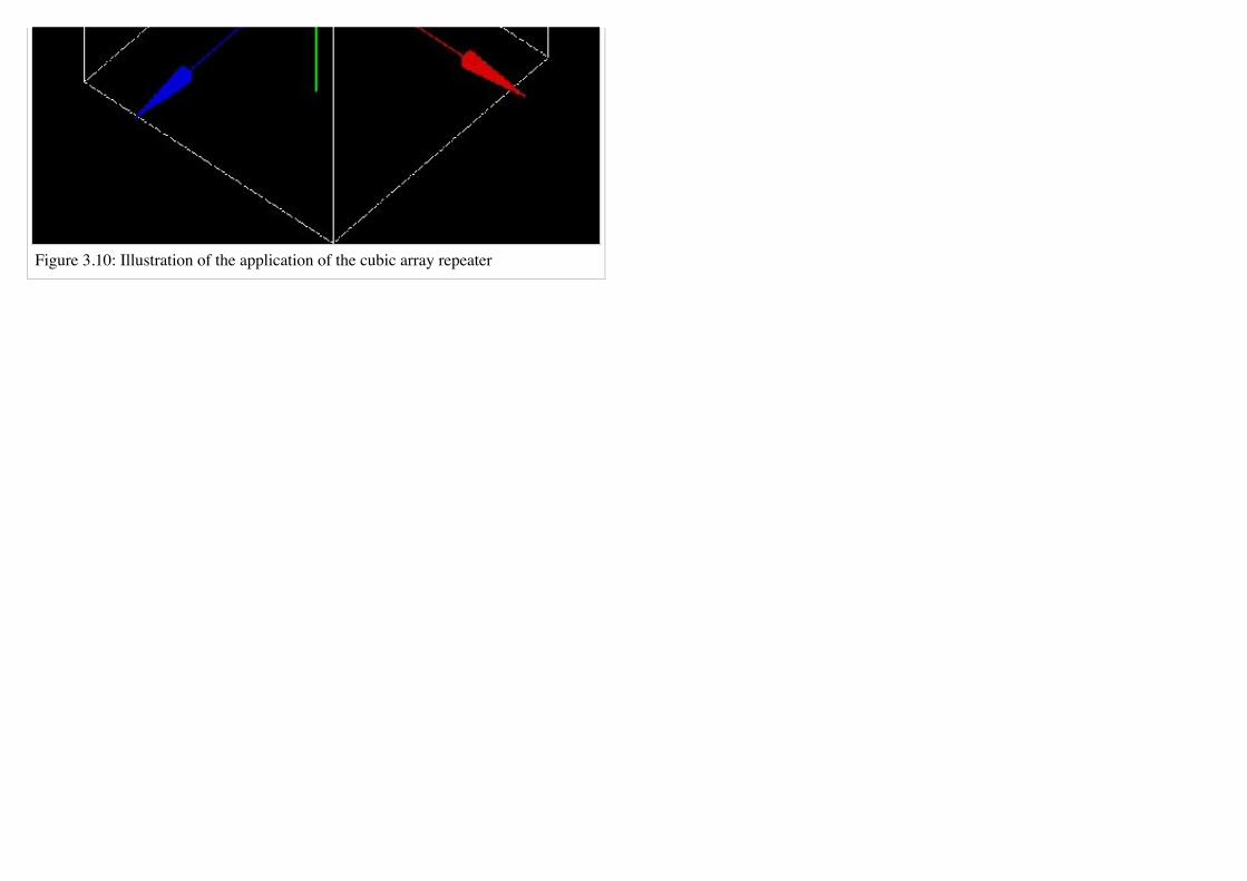
Figure 3.10: Illustration of the application of the cubic array repeater

Figure 3.10B: Illustration of the application of the cubic array repeater (after)

Quadrant repeater

The quadrant repeater is appropriate to repeat a volume in a triangle-like pattern similar to that of a Derenzo resolution phantom.

To select the quadrant repeater, use:

/gate/Name_Volume/repeaters/insert quadrant

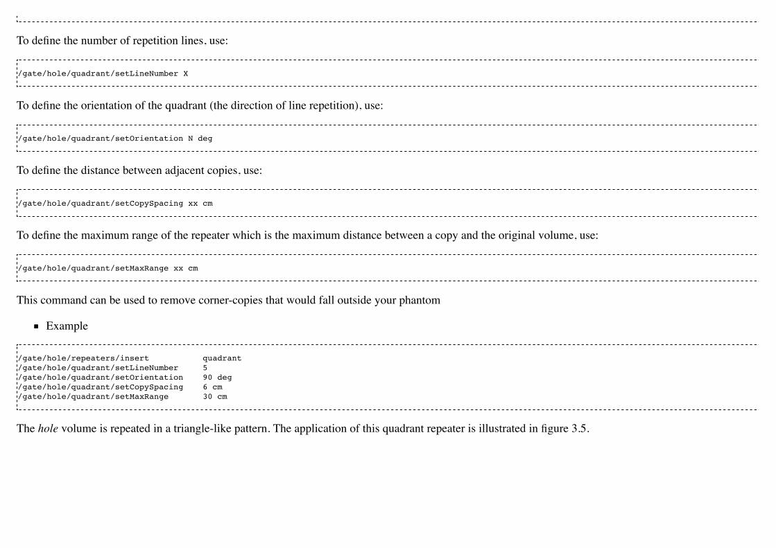
To define the number of repetition lines, use:

/gate/hole/quadrant/setLineNumber X

To define the orientation of the quadrant (the direction of line repetition), use:

/gate/hole/quadrant/setOrientation N deg

To define the distance between adjacent copies, use:

/gate/hole/quadrant/setCopySpacing xx cm

To define the maximum range of the repeater which is the maximum distance between a copy and the original volume, use:

/gate/hole/quadrant/setMaxRange xx cm

This command can be used to remove corner-copies that would fall outside your phantom

Example

/gate/hole/repeaters/insert quadrant /gate/hole/quadrant/setLineNumber 5 /gate/hole/quadrant/setOrientation 90 deg /gate/hole/quadrant/setCopySpacing 6 cm /gate/hole/quadrant/setMaxRange 30 cm

The hole volume is repeated in a triangle-like pattern. The application of this quadrant repeater is illustrated in figure 3.5.

Figure 3.10: Illustration of the application of the cubic array repeater

Figure 3.10b: Illustration of the application of the cubic array repeater (after)

Remark: The repeaters that are applied to the Name_Volume volume can be listed using:

/gate/Name_Volume/repeaters/list

Sphere repeater

The sphere repeater makes it possible to repeat a volume along a spherical ring. It is useful to build rings of detectors for PET scanners having gantry ofspherical shape (e.g. SIEMENS Ecat Accel, Hi-Rez, ....)

To select the sphere repeater, use:

/gate/Name_Volume/repeaters/insert sphere

Then, the radius R of the sphere can be set using:

/gate/Name_Volume /sphere/setRadius X cm

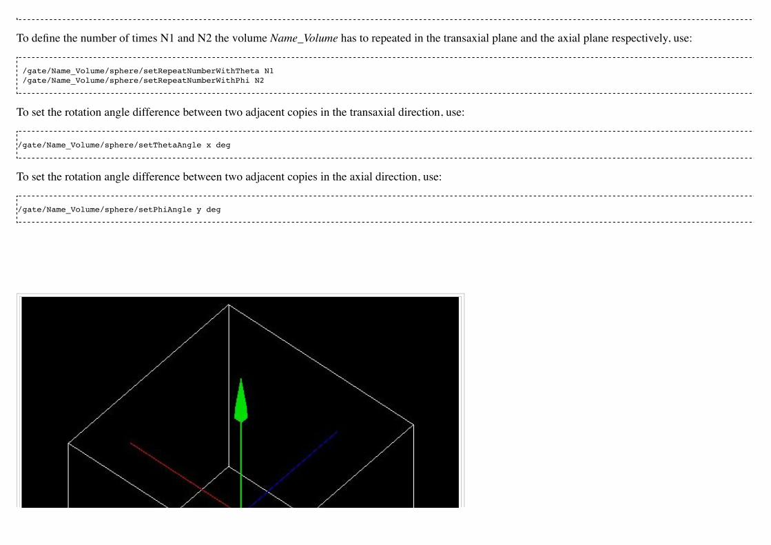
To define the number of times N1 and N2 the volume Name_Volume has to repeated in the transaxial plane and the axial plane respectively, use:

/gate/Name_Volume/sphere/setRepeatNumberWithTheta N1 /gate/Name_Volume/sphere/setRepeatNumberWithPhi N2

To set the rotation angle difference between two adjacent copies in the transaxial direction, use:

/gate/Name_Volume/sphere/setThetaAngle x deg

To set the rotation angle difference between two adjacent copies in the axial direction, use:

/gate/Name_Volume/sphere/setPhiAngle y deg

Figure 3.12: Illustration of the application of the sphere repeater

The replicates of the volume Name_Volume will be placed so that its axis remains tangential to the ring.

Example 3.12

/gate/block/repeaters/insert sphere /gate/block/sphere/setRadius 25. cm /gate/block/sphere/setRepeatNumberWithTheta 10 /gate/block/sphere/setRepeatNumberWithPhi 3 /gate/block/setThetaAngle 36 deg /gate/block/setThetaAngle 20 deg

The block volume is repeated 10 times along the transaxial plane, with a rotation angle between two neighbouring blocks of 36 deg, and is repeated 3 timesin the axial direction with a rotation angle between two neighbouring blocks of 20 deg. The sphere defined here has a 25 cm radius.

Generic repeater

It is also possible to repeat a volume according to a list of transformations (rotation and translation). The following macros read the transformations into asimple text file:

/gate/myvolume/repeaters/insert genericRepeater/gate/myvolume/genericRepeater/setPlacementsFilename data/myvolume.placements/gate/myvolume/genericRepeater/useRelativeTranslation 1

The text file "myvolume.placements" is composed as follows:

###### List of placement (translation and rotation) ###### Column 1 is rotationAngle in degree ###### Columns 2,3,4 are rotation axis ###### Columns 5,6,7 are translation in mmRotation deg Translation mm0 0 1 0 0 0 1010 0 1 0 0 0 1015 0 1 0 0 0 20

line with # are ignoredfirst word must be Rotation or Translation followed with the unity (deg and mm here)Rotation are described with 4 columns, the first for the angle, three others for the rotation axisTranslation are described with X Y Z.using "useRelativeTranslation 1" (default) allows to compose the transformation according to the initial volume translation. If set to 0, thetransformation is set as is (in the coordinate system of the mother volume).

See example here

Placing a volumeThe position of the volume in the geometry is defined using the sub-tree

/placement/

Three types of placement are available: translation, rotation and alignment.

Translation

To translate the Name_Volume volume along the X direction by x cm, the command is:

/gate/Name_Volume/placement/setTranslation x. 0. 0. cm

The position is always given with respect to the center of the mother volume.

To set the Phi angle (in XY plane) of the translation vector, use:

/gate/Name_Volume/placement/setPhiOfTranslation N deg

To set the Theta angle (with regard to the Z axis) of the translation vector, use:

/gate/Name_Volume/placement/setThetaOfTranslation N deg

To set the magnitude of the translation vector, use:

/gate/Name_Volume/placement/setMagOfTranslation xx cm

Example

/gate/Phantom/placement/setTranslation 1. 0. 0. cm /gate/Phantom/placement/setMagOfTranslation 10. cm

The Phantom volume is placed at 10 cm, 0 cm and 0 cm from the center of the mother volume (here the world volume). The application of this translationplacement is illustrated in figure 3.13.

Rotation

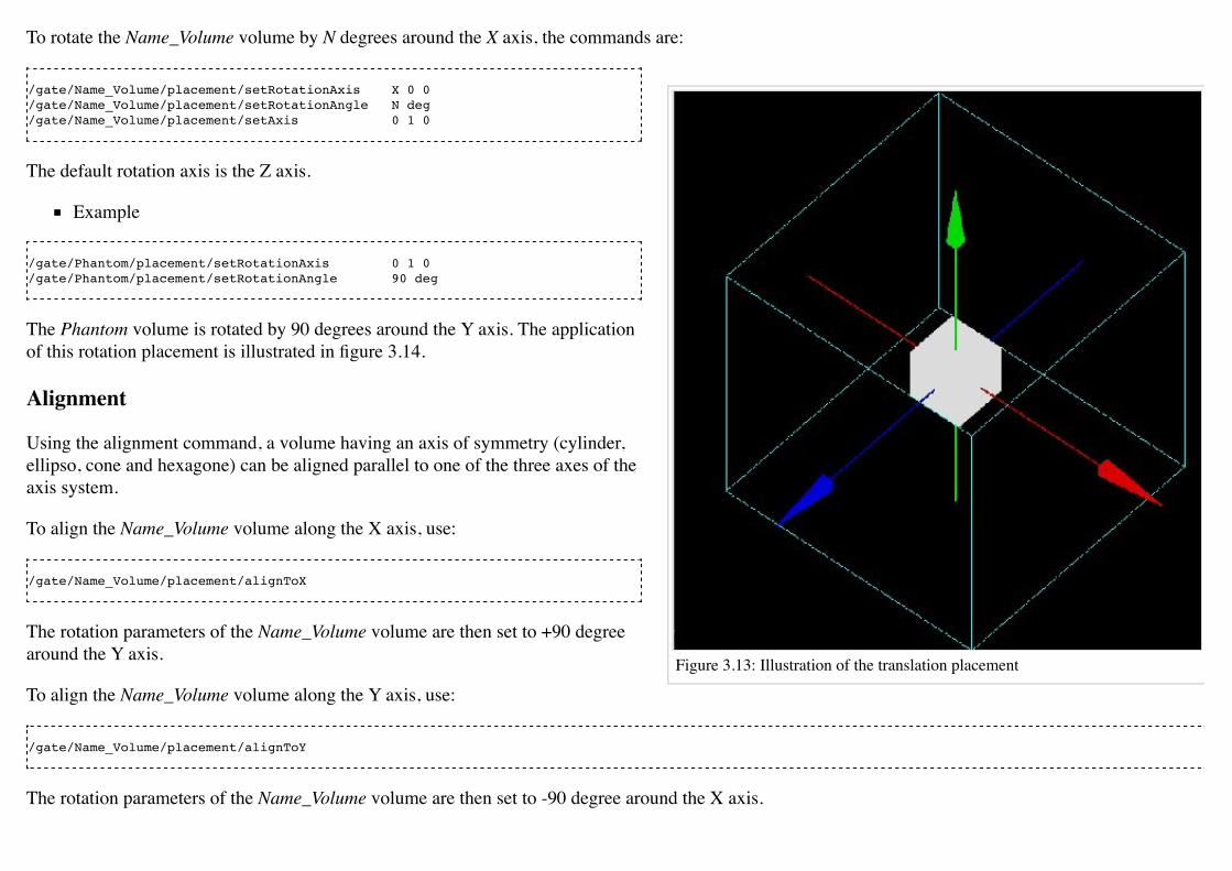
Figure 3.13: Illustration of the translation placement

To rotate the Name_Volume volume by N degrees around the X axis, the commands are:

/gate/Name_Volume/placement/setRotationAxis X 0 0 /gate/Name_Volume/placement/setRotationAngle N deg /gate/Name_Volume/placement/setAxis 0 1 0

The default rotation axis is the Z axis.

Example

/gate/Phantom/placement/setRotationAxis 0 1 0 /gate/Phantom/placement/setRotationAngle 90 deg

The Phantom volume is rotated by 90 degrees around the Y axis. The applicationof this rotation placement is illustrated in figure 3.14.

Alignment

Using the alignment command, a volume having an axis of symmetry (cylinder,ellipso, cone and hexagone) can be aligned parallel to one of the three axes of theaxis system.

To align the Name_Volume volume along the X axis, use:

/gate/Name_Volume/placement/alignToX

The rotation parameters of the Name_Volume volume are then set to +90 degreearound the Y axis.

To align the Name_Volume volume along the Y axis, use:

/gate/Name_Volume/placement/alignToY

The rotation parameters of the Name_Volume volume are then set to -90 degree around the X axis.

Illustration of the translation placement

To align the Name_Volume volume along the Z axis (default axis of rotation) use:

/gate/Name_Volume/placement/alignToZ

The rotation parameters of the Name_Volume volume are then set to 0 degree.

Special example: Wedge volume and OPET scanner

The wedge is always created as shown in figure 3.4, that is with the slantedplane oriented towards the positive X direction. If one needs to have itoriented differently, one could, for instance, rotate it:

/gate/wedge0/placement/setRotationAxis 0 1 0 /gate/wedge0/placement/setRotationAngle 180 deg

The center of a wedge in the Y and Z directions are simply

respectively. For the X direction, the center is located such that

where Delta is the length of the wedge across the middle of the Y direction, asshown in Figure 3.15.

Figure 3.14: Illustration of the rotation placement

Figure 3.15: Center of wedge

Wedge crystals are used to build the OPET scanner, in which the scanner ringgeometry approximates a true circular ring.

By knowing the radius gantry R and the length of the longest crystal, it ispossible to arrange a series of 8 crystals with varying the lengths as shown inFigure 3.16.

It is first necessary to create by-hand the first row of crystals. This isaccomplished by first creating a module just big enough to contain one rowof wedge crystals.

/gate/rsector/daughters/name module /gate/rsector/daughters/insert box /gate/module/geometry/setXLength 10 mm /gate/module/geometry/setYLength 17.765 mm /gate/module/geometry/setZLength 2.162 mm /gate/module/setMaterial Air

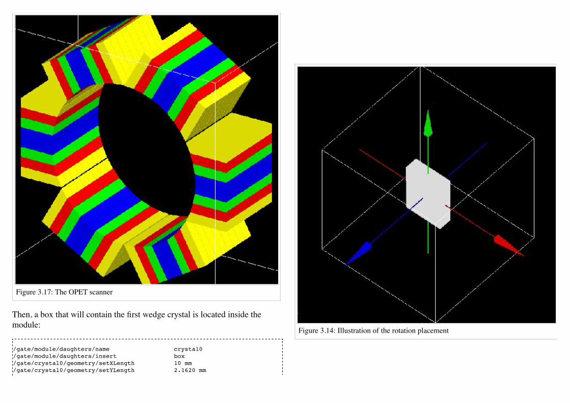
Figure 3.14: Illustration of the rotation placement

Figure 3.17: The OPET scanner

Then, a box that will contain the first wedge crystal is located inside themodule:

/gate/module/daughters/name crystal0 /gate/module/daughters/insert box /gate/crystal0/geometry/setXLength 10 mm /gate/crystal0/geometry/setYLength 2.1620 mm

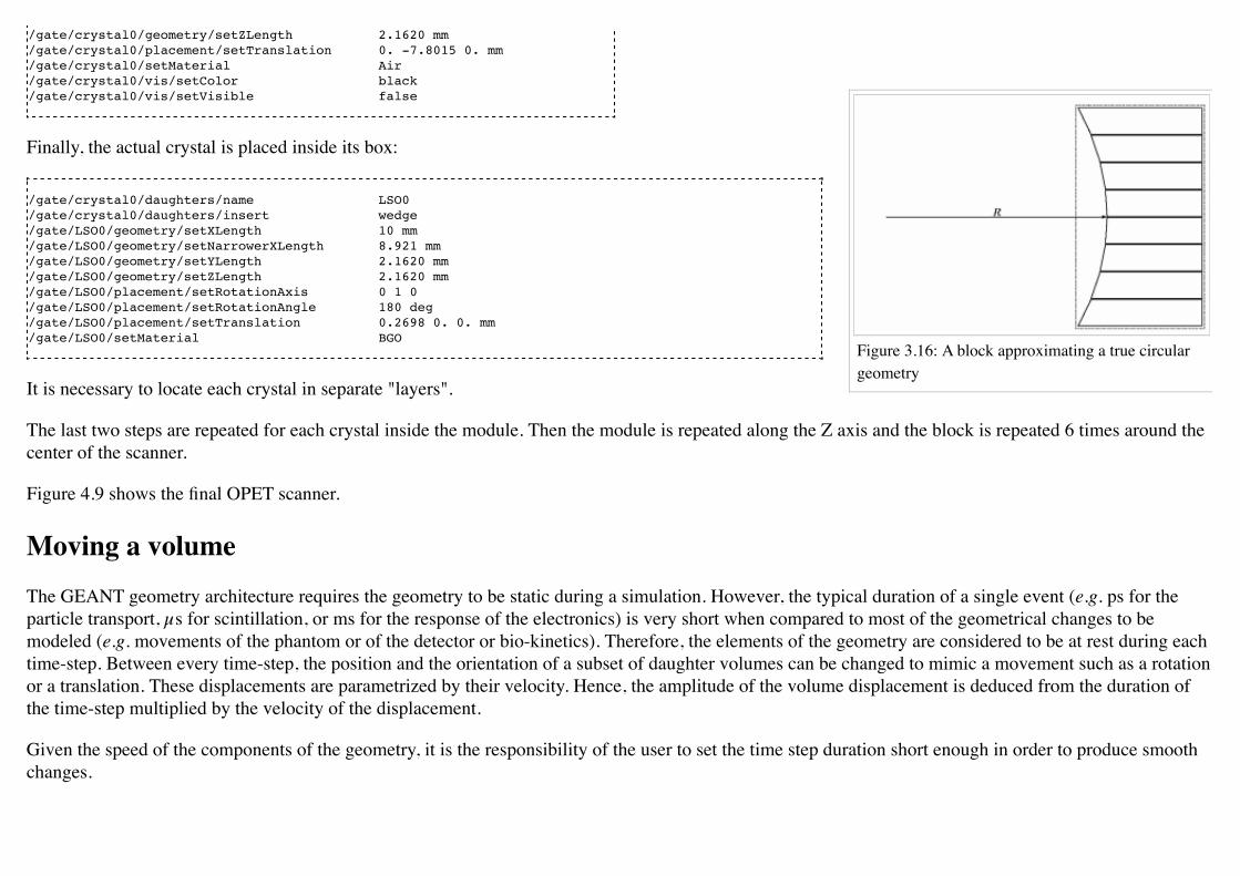
Figure 3.16: A block approximating a true circulargeometry

/gate/crystal0/geometry/setZLength 2.1620 mm /gate/crystal0/placement/setTranslation 0. -7.8015 0. mm /gate/crystal0/setMaterial Air /gate/crystal0/vis/setColor black /gate/crystal0/vis/setVisible false

Finally, the actual crystal is placed inside its box:

/gate/crystal0/daughters/name LSO0 /gate/crystal0/daughters/insert wedge /gate/LSO0/geometry/setXLength 10 mm /gate/LSO0/geometry/setNarrowerXLength 8.921 mm /gate/LSO0/geometry/setYLength 2.1620 mm /gate/LSO0/geometry/setZLength 2.1620 mm /gate/LSO0/placement/setRotationAxis 0 1 0 /gate/LSO0/placement/setRotationAngle 180 deg /gate/LSO0/placement/setTranslation 0.2698 0. 0. mm /gate/LSO0/setMaterial BGO

It is necessary to locate each crystal in separate "layers".

The last two steps are repeated for each crystal inside the module. Then the module is repeated along the Z axis and the block is repeated 6 times around thecenter of the scanner.

Figure 4.9 shows the final OPET scanner.

Moving a volumeThe GEANT geometry architecture requires the geometry to be static during a simulation. However, the typical duration of a single event (e.g. ps for theparticle transport, µs for scintillation, or ms for the response of the electronics) is very short when compared to most of the geometrical changes to bemodeled (e.g. movements of the phantom or of the detector or bio-kinetics). Therefore, the elements of the geometry are considered to be at rest during eachtime-step. Between every time-step, the position and the orientation of a subset of daughter volumes can be changed to mimic a movement such as a rotationor a translation. These displacements are parametrized by their velocity. Hence, the amplitude of the volume displacement is deduced from the duration ofthe time-step multiplied by the velocity of the displacement.

Given the speed of the components of the geometry, it is the responsibility of the user to set the time step duration short enough in order to produce smoothchanges.

A volume can be moved during a simulation using five types of motion: rotation, translation, orbiting, wobbling and eccentric rotation, as explained below.

Translation

To translate a Name_Volume volume during the simulation, the commands are:

/gate/Name_Volume/moves/insert translation /gate/Name_Volume/translation/setSpeed x 0 0 cm/s

where x is the speed of translation and the translation is performed along the X axis. These commands can be useful to simulate table motion during a scanfor instance.

Example

/gate/Table/moves/insert translation /gate/Table/translation/setSpeed 0 0 1 cm/s

The Table volume is translated along the Z axis with a speed of 1 cm per second.

Rotation

To rotate a Name_Volume volume around an axis during the simulation, with a speed of N degrees per second, the commands are:

/gate/Name_Volume/moves/insert rotation /gate/Name_Volume/rotation/setSpeed N deg/s /gate/Name_Volume/rotation/setAxis 0 y 0

Example

/gate/Phantom/moves/insert rotation /gate/Phantom/rotation/setSpeed 1 deg/s /gate/Phantom/rotation/setAxis 0 1 0

The Phantom volume rotates around the Y axis with a speed of 1 degree per second.

Orbiting

Rotating a volume around any axis during a simulation is possible using the orbiting motion. This motion is needed to model the camera head rotation inSPECT. To rotate the Name_Volume volume around the X axis with a speed of N degrees per second, the commands are:

/gate/SPECThead/moves/insert orbiting /gate/SPECThead/orbiting/setSpeed N. deg/s /gate/SPECThead/orbiting/setPoint1 0 0 0 cm /gate/SPECThead/orbiting/setPoint2 1 0 0 cm

The last two commands define the rotation axis.

It is possible to enable or disable the volume auto-rotation option using:

/gate/Name_Volume/orbiting/enableAutoRotation /gate/Name_Volume/orbiting/disableAutoRotation

Example

/gate/camera_head/moves/insert orbiting /gate/camera_head/orbiting/setSpeed 1. deg/s /gate/camera_head/orbiting/setPoint1 0 0 0 cm /gate/camera_head/orbiting/setPoint2 0 0 1 cm

The camera_head volume is rotated around the Z axis during the simulation with a speed of 1 degree per second.

Wobbling

The wobbling motion enables an oscillating translation movement to the volume.

This motion is needed to mimic the behavior of certain PET scanners that wobble to increase the spatial sampling of the data during the acquisition.

The movement that is modeled is defined by where dM(t) is the translation vector at time t, A is the maximumdisplacement vector, f is the movement frequency, phi is the phase at t=0, and t is the time.

To set the parameters of that equation, use:

/gate/Name_Volume/moves/insert osc-trans

To set the amplitude vector of the oscillating translation:

/gate/Name_Volume/osc-trans/setAmplitude x. 0. 0. cm

To set the frequency of the oscillating translation:

/gate/Name_Volume/osc-trans/setFrequency N Hz

To set the period of the oscillating translation:

/gate/Name_Volume/osc-trans/setPeriod N s

To set the phase at t=0 of the oscillating translation:

/gate/Name_Volume/osc-trans/setPhase N deg

Example

/gate/crystal/moves/insert osc-trans /gate/crystal/osc-trans/setAmplitude 10. 0. 0. cm /gate/crystal/osc-trans/setFrequency 50 Hz /gate/crystal/osc-trans/setPeriod 1 s /gate/crystal/osc-trans/setPhase 90 deg

In this example, the movement that is modeled is defined by

Eccentric rotation

The eccentric rotation motion enables an eccentric rotation movement of the volume. It is a particular case of the orbiting movement. To set the object ineccentric position (X-Y-Z) and rotate it around the OZ lab frame axis, use:

/gate/Name_Volume/moves/insert eccent-rot

To set the shifts in the X-Y-Z directions:

/gate/Name_Volume/eccent-rot/setShiftXYZ x y z cm

To set the orbiting angular speed:

/gate/Name_Volume/eccent-rot/setSpeed N deg/s

Remark : This particular move is closely related to the LMF definition since the move parameters (shifts in all 3 directions and angular speed) arepropagated in the .cch header.

Example

/gate/crystal/moves/insert eccent-rot /gate/crystal/eccent-rot/setShiftXYZ 5. 0. 0. cm /gate/crystal/eccent-rot/setSpeed 10 deg/s

The crystal volume is placed at 10 cm, 0 cm and 0 cm from the center of its mother volume and will rotate around the Z axis during the simulation with aspeed of 10 degrees per second.

Generic move

A volume can be move at given time value thanks to the following macros:

/gate/myvolume/moves/insert genericMove/gate/myvolume/genericMove/setPlacementsFilename data/myvolume.placements

In the same idea than GenericRepeater,the placements file contains the transformations (rotation, translation) and the time value where this transformationsis applied.

###### List of placement (translation and rotation) according to time ###### Column 1 is Time in s (second)###### Column 2 is rotationAngle in degree###### Columns 3,4,5 are rotation axis ###### Columns 6,7,8 are translation in mmTime s Rotation deg Translation mm0 0 0 1 0 0 0 100250.7 3 0 1 0 0 10 100492.9 4 0 1 0 0 20 100742.9 8 0 1 0 30 0 100

WARNING. The time values given here do not necessarily correspond to simulation's run. The real runs are defined with the time slices (see this section forexample). At each new run, GATE looks into the time-placements list and chooses the one that corresponds to the starting time of the run. It leads that someplacements can be not applied (if one run start before the placement time and the next run start after the next placement time). If run time is after the lastplacements time in the list, the last placements is applied.

See example here

Generic repeater move

You can combine generic repeater and generic move to allow different repeated configurations according to time. This is for example useful to describemulti-leaf collimator from a single leaf which is repeated at different positions, and which move according to each beam.

/gate/myvolume/moves/insert genericRepeaterMove/gate/myvolume/genericRepeaterMove/setPlacementsFilename data/myvolume.placements/gate/myvolume/genericRepeaterMove/useRelativeTranslation 1

###### List of placement (translation and rotation)###### Column 1 is rotationAngle in degree###### Columns 2,3,4 are rotation axis###### Columns 5,6,7 are translation in mmTime sNumberOfPlacements 3

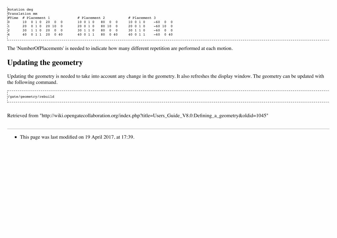
Rotation degTranslation mm#Time # Placement 1 # Placement 2 # Placement 30 10 0 1 0 20 0 0 10 0 1 0 80 0 0 10 0 1 0 -60 0 01 20 0 1 0 20 10 0 20 0 1 0 80 10 0 20 0 1 0 -60 10 02 30 1 1 0 20 0 0 30 1 1 0 80 0 0 30 1 1 0 -60 0 04 40 0 1 1 20 0 40 40 0 1 1 80 0 40 40 0 1 1 -60 0 40

The 'NumberOfPlacements' is needed to indicate how many different repetition are performed at each motion.

Updating the geometryUpdating the geometry is needed to take into account any change in the geometry. It also refreshes the display window. The geometry can be updated withthe following command.

/gate/geometry/rebuild

Retrieved from "http://wiki.opengatecollaboration.org/index.php?title=Users_Guide_V8.0:Defining_a_geometry&oldid=1045"

This page was last modified on 19 April 2017, at 17:39.

Users Guide V8.0:MaterialsFrom Wiki OpenGATE

Contents1 The Gate material database

1.1 Elements1.2 Materials

2 Modifying the Gate material database2.1 New element2.2 New material

2.2.1 Elements as materials2.2.2 Compounds as materials2.2.3 Mixtures as materials2.2.4 Mixtures of materials as materials

3 Ionization potential

The Gate material databaseThe primary method for defining the properties of the materials used in Gate is by a materials database. This file holds all the information required for Gateto assign the nuclear properties from the Geant4 data sets, and is easily modified by the user. The OpenGate collaboration supplies a fairly extensive listingof materials in this file as part of Gate. This chapter describes the details of how to modify this database.

As alluded to in the previous paragraph, there exists an alternate method for materials definitions. As discussed in previous chapters, Gate scripts aredeveloped from Geant4 C++ data classes in order to simplify and standardize input for Geant4. As a result, materials definitions can be written and compiledin C++ directly using the Geant4 tools. Specifying materials in this manner is beyond the scope of this document. For those interested in direct access toGeant4's materials should refer to the Geant4 User's Guide: For Application Developers and the Geant4 User's Guide: For Toolkit Developers for moredetailed information.

The material database contains two Geant4 structures called elements and materials that are used to define the physical properties of the atoms, molecules,and compounds. In contrast with Geant4, Gate does not use isotopic abundances. This omission has little bearing on Gate applications because isotopicabundances are unimportant in low to mid energy photon and charged particle interactions. In fact, this distinction is only important for enriched or depletedmaterials interacting with neutrons or, high energy (>5 MeV) photons or charged particles.

It is possible to use several material database. If a material is defined in several database, Gate keeps the material in last database called (with a warningmessage). To call a database:

/gate/geometry/setMaterialDatabase MyMaterialDatabase.db

Elements

Elements are the building blocks of all the materials used in Gate simulations. Elements in Gate are defined as in a periodic table. Gate stores the elementsname, symbol, atomic number, and molar mass. As stated above, isotopic abundances are not referenced or used. The supplied file GateMaterials.dbcontains the most commonly used elements and their molar masses as they are found in nature.

Some elements, particularly those that have an isotope with a large cross section for neutron absorption, have isotopic abundances and thus molar massesthat vary depending upon their source. One element that exhibits this behavior is boron. In practice this behavior is not important for Gate applications.

Materials

In Gate, materials are defined as combinations of elements, and are an important parameter that Gate uses for all of the particle interactions that take placeduring a simulation. These combinations of elements require defining four additional parameters. These are the material's name, density, constituentelement(s), and their individual abundances.

The composition of elements within a material can be defined in two different ways. If the material is a chemical compound then its relative amounts ofelements are specified by the number of atoms in the chemical formula of the compound. For example, methane would be defined as having onecarbon atom and four hydrogen atoms. If the material is better described as a mixture, such as 304-stainless steel, then the relative combinations of theelements are given by mass fraction. In the case of 304-stainless steel, the various mass fractions are given as 0.695 Iron, 0.190 Chromium, 0.095 Nickel,and 0.020 Manganese. Note that the mass fractions from the elements must all sum to one.

Densities of materials often vary greatly between different sources and must be carefully selected for the specific application in mind. Units of density mustalso be defined. These are typically given in g/cm3 but can be given in more convenient units for extreme cases. For example, a vacuum's density may beexpressed in units of mg/cm3.

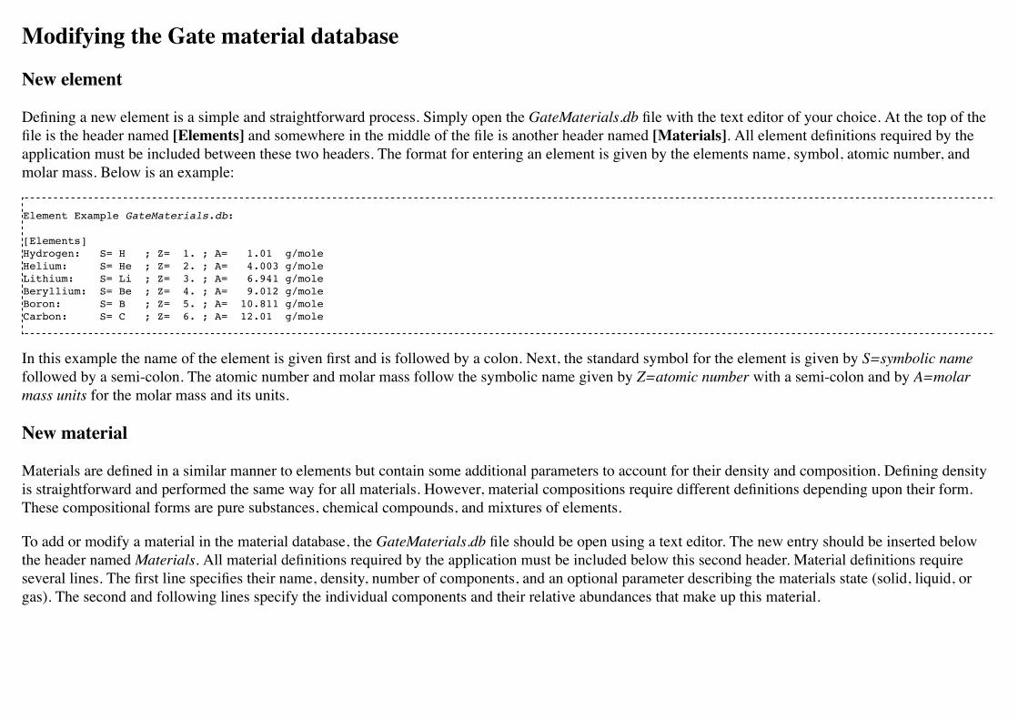
Modifying the Gate material database

New element

Defining a new element is a simple and straightforward process. Simply open the GateMaterials.db file with the text editor of your choice. At the top of thefile is the header named [Elements] and somewhere in the middle of the file is another header named [Materials]. All element definitions required by theapplication must be included between these two headers. The format for entering an element is given by the elements name, symbol, atomic number, andmolar mass. Below is an example:

Element Example GateMaterials.db:

[Elements]Hydrogen: S= H ; Z= 1. ; A= 1.01 g/mole Helium: S= He ; Z= 2. ; A= 4.003 g/moleLithium: S= Li ; Z= 3. ; A= 6.941 g/moleBeryllium: S= Be ; Z= 4. ; A= 9.012 g/moleBoron: S= B ; Z= 5. ; A= 10.811 g/moleCarbon: S= C ; Z= 6. ; A= 12.01 g/mole

In this example the name of the element is given first and is followed by a colon. Next, the standard symbol for the element is given by S=symbolic namefollowed by a semi-colon. The atomic number and molar mass follow the symbolic name given by Z=atomic number with a semi-colon and by A=molarmass units for the molar mass and its units.

New material

Materials are defined in a similar manner to elements but contain some additional parameters to account for their density and composition. Defining densityis straightforward and performed the same way for all materials. However, material compositions require different definitions depending upon their form.These compositional forms are pure substances, chemical compounds, and mixtures of elements.

To add or modify a material in the material database, the GateMaterials.db file should be open using a text editor. The new entry should be inserted belowthe header named Materials. All material definitions required by the application must be included below this second header. Material definitions requireseveral lines. The first line specifies their name, density, number of components, and an optional parameter describing the materials state (solid, liquid, orgas). The second and following lines specify the individual components and their relative abundances that make up this material.

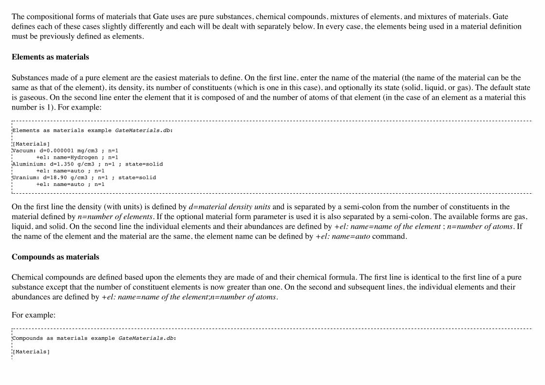
The compositional forms of materials that Gate uses are pure substances, chemical compounds, mixtures of elements, and mixtures of materials. Gatedefines each of these cases slightly differently and each will be dealt with separately below. In every case, the elements being used in a material definitionmust be previously defined as elements.

Elements as materials

Substances made of a pure element are the easiest materials to define. On the first line, enter the name of the material (the name of the material can be thesame as that of the element), its density, its number of constituents (which is one in this case), and optionally its state (solid, liquid, or gas). The default stateis gaseous. On the second line enter the element that it is composed of and the number of atoms of that element (in the case of an element as a material thisnumber is 1). For example:

Elements as materials example GateMaterials.db:

[Materials]Vacuum: d=0.000001 mg/cm3 ; n=1 +el: name=Hydrogen ; n=1Aluminium: d=1.350 g/cm3 ; n=1 ; state=solid +el: name=auto ; n=1Uranium: d=18.90 g/cm3 ; n=1 ; state=solid +el: name=auto ; n=1

On the first line the density (with units) is defined by d=material density units and is separated by a semi-colon from the number of constituents in thematerial defined by n=number of elements. If the optional material form parameter is used it is also separated by a semi-colon. The available forms are gas,liquid, and solid. On the second line the individual elements and their abundances are defined by +el: name=name of the element ; n=number of atoms. Ifthe name of the element and the material are the same, the element name can be defined by +el: name=auto command.

Compounds as materials

Chemical compounds are defined based upon the elements they are made of and their chemical formula. The first line is identical to the first line of a puresubstance except that the number of constituent elements is now greater than one. On the second and subsequent lines, the individual elements and theirabundances are defined by +el: name=name of the element;n=number of atoms.

For example:

Compounds as materials example GateMaterials.db:

[Materials]

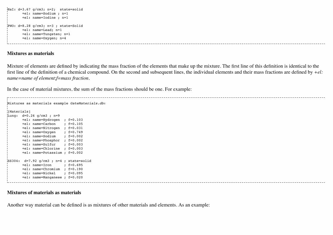
NaI: d=3.67 g/cm3; n=2; state=solid +el: name=Sodium ; n=1 +el: name=Iodine ; n=1

PWO: d=8.28 g/cm3; n=3 ; state=Solid +el: name=Lead; n=1 +el: name=Tungsten; n=1 +el: name=Oxygen; n=4

Mixtures as materials

Mixture of elements are defined by indicating the mass fraction of the elements that make up the mixture. The first line of this definition is identical to thefirst line of the definition of a chemical compound. On the second and subsequent lines, the individual elements and their mass fractions are defined by +el:name=name of element;f=mass fraction.

In the case of material mixtures, the sum of the mass fractions should be one. For example:

Mixtures as materials example GateMaterials.db:

[Materials]Lung: d=0.26 g/cm3 ; n=9 +el: name=Hydrogen ; f=0.103 +el: name=Carbon ; f=0.105 +el: name=Nitrogen ; f=0.031 +el: name=Oxygen ; f=0.749 +el: name=Sodium ; f=0.002 +el: name=Phosphor ; f=0.002 +el: name=Sulfur ; f=0.003 +el: name=Chlorine ; f=0.003 +el: name=Potassium ; f=0.002

SS304: d=7.92 g/cm3 ; n=4 ; state=solid +el: name=Iron ; f=0.695 +el: name=Chromium ; f=0.190 +el: name=Nickel ; f=0.095 +el: name=Manganese ; f=0.020

Mixtures of materials as materials

Another way material can be defined is as mixtures of other materials and elements. As an example:

Mixtures of mixtures as materials example GateMaterials.db:

[Materials]Aerogel: d=0.200 g/cm3 ; n=3 +mat: name=SiO2 ; f=0.625 +mat: name=Water ; f=0.374 +el: name=Carbon ; f=0.001

In this example, the material, Aerogel, is defined to be made up of two materials, silicon dioxide and water, and one element, carbon. Mass fractions of thesilicon dioxide, water, and carbon are given to specify the atom densities of the material when related to the density of the Aerogel. When specifyingmaterials rather than elements the +mat: name=identifier must be used.

Ionization potentialThe ionization potential is the energy required to remove an electron to an atom or a molecule. By default, the ionization potential is calculated thanks to theBragg’s additivity rule. It is possible to define the ionization potential of each material defined in gate. For example:

/gate/geometry/setIonisationPotential Water 75 eV

Retrieved from "http://wiki.opengatecollaboration.org/index.php?title=Users_Guide_V8.0:Materials&oldid=252"


Users Guide V8.0:Setting up the physicsFrom Wiki OpenGATE

Contents1 New physics list mechanism2 Physics list selection

2.1 Particles2.2 Adding a process2.3 Removing a process2.4 Models and Data sets

3 Physics processes3.1 Electromagnetic processes

3.1.1 Photoelectric effect3.1.2 Compton scattering3.1.3 Rayleigh scattering3.1.4 Pair production3.1.5 Ionization3.1.6 Bremsstrahlung3.1.7 Positron and electron annihilation3.1.8 Single and multiple Scattering3.1.9 Muon electromagnetic processes3.1.10 Electromagnetic options

3.2 Hadronic processes3.2.1 Main Geant4 models3.2.2 Elastic scattering3.2.3 Inelastic process for proton3.2.4 Inelastic process for ion3.2.5 Pions3.2.6 Neutrons3.2.7 Particle decay3.2.8 Radioactive decay

3.3 Optical physics processes3.3.1 Bulk Absorption3.3.2 Rayleigh Scattering3.3.3 Mie Scattering3.3.4 Processes at Boundaries3.3.5 Wavelength Shifting or Fluorescence

4 Magnetic field

New physics list mechanismWARNING : big change from Gate V7.0

Up to now, physic lists were set in GATE according to macro files containing list of command to add physical processes. From GATE Version 7.0, we highlyrecommend to switch to the "physic list builder" mechanism. The physic-list builders are provided by the Geant4 community. To use a builder, use the"addPhyslicsList" command as follow :

/gate/physics/addPhysicsList QGSP_BERT_EMV

The name of the builder is one of the following for the electromagnetic physic-lists:

emstandardemstandard_opt1emstandard_opt2emstandard_opt3emlivermoreemlivermore_polarempenelope

And for the hadronic physics list builders :

QGSPQGSP_EMVQGSCQGSC_EMV

QGSP_EFLOWQGSP_BERTQGSP_BERT_EMVQGSP_BERT_HPQGSP_BERT_TRVQGSP_BICQGSP_BIC_HPQGSP_NEQQGSP_EMV_NQEQGSP_BERT_NQEQGSP_INCLXXFTFP_BERTFTFPFTFP_EMV...

See more details on electromagnetic (http://geant4.web.cern.ch/geant4/collaboration/working_groups/electromagnetic/physlist9.5.shtml) and hadronic(http://geant4.web.cern.ch/geant4/support/proc_mod_catalog/physics_lists/referencePL.shtml) builders. Another guide can be found here(http://geant4.in2p3.fr/IMG/pdf_PhysicsLists.pdf).

The production cuts special cuts can still be used as exemplified below :

/gate/physics/Gamma/SetCutInRegion world 10 mm/gate/physics/Electron/SetCutInRegion world 10 mm/gate/physics/Positron/SetCutInRegion world 10 mm/gate/physics/Proton/SetCutInRegion world 10 mm

/gate/physics/Gamma/SetCutInRegion patient 1 mm/gate/physics/Electron/SetCutInRegion patient 1 mm/gate/physics/Positron/SetCutInRegion patient 1 mm/gate/physics/Proton/SetCutInRegion patient 1 mm

/gate/physics/SetMaxStepSizeInRegion patient 1 mm/gate/physics/ActivateStepLimiter proton

Physics list selection

Processes have three possible states: "Available", "Enabled" and "Initialized". In a simulation, GATE uses initialized processes. By default, all processes areonly "Available". To initialize processes you want to use, you have to choose them in the list of available processes and put them in the list of "Enabled"processes with the addProcess/removeProcess commands. Then, you have to define models, data sets or energy range if it is necessary. Enabled processesare initialized when the command /gate/run/initialize is called. After initialization, physics list cannot be modified. Processes must be initialized before thesource definition.

To obtain the list of processes available, enabled or initialized:

/gate/physics/processList [State] [Particle]

Parameter : StateParameter type : sOmittable : TrueDefault value : AvailableCandidates : Available Enabled Initialized

Parameter : ParticleParameter type : sOmittable : TrueDefault value : All

User can print the list of initialized processes for each particles and the list of enabled processes with all informations (particles, models, data sets and energyrange):

/gate/physics/print [File name]

Parameter : File NameParameter type : sOmittable : False

Particles

To designate a particle in a macro command for physics, you have to use the Geant4 name of the particle. The command /particle/list gives the list ofparticles available in GATE. Note that there are 5 particles defined for nuclei: "deuteron", "triton", "alpha", "He3" and a generic particle for all ions called"GenericIon". For more information about particles in Geant4, see Geant4 user support[1].

User can also use a particle group name. For example, "Charged" designates all charged particles or “EM” designates gamma, e+ and e-. Here, the list ofparticle groups available in GATE:

Default : defaults particles defined for a process (see the "processList" command before for more informations)EM : e+, e-, gammaCharged : all charged particles

< ! > Particle name in non-physics macro command could be slightly different in particular for ions!

Adding a process

To add a process to the list of "Enabled" processes for a particle or a group of particles:

/gate/physics/addProcess [Process] [Particle]

Parameter : ProcessParameter type : sOmittable : False

Parameter : Particle Parameter type : sOmittable : TrueDefault value : Default

Removing a process

To remove a process of the "Enabled" processes list:

/gate/physics/removeProcess [Process] [Particle]

Parameter : ProcessParameter type : sOmittable : False

Parameter : ParticleParameter type : sOmittable : TrueDefault value : Default

Models and Data sets

Some processes have several models or several data sets available. To known if you can choose a model or a data set for a process, use the commands:

/gate/physics/processes/[Process Name]/modelList [Particle]/gate/physics/processes/[Process Name]/dataSetList [Particle]


To select or unselect a model or a data set, use the command:

/gate/physics/processes/[Process Name]/setModel [Model Name] [Particle]/gate/physics/processes/[Process Name]/unSetModel [Model Name] [Particle]/gate/physics/processes/[Process Name]/setDataSet [DataSet Name] [Particle]/gate/physics/processes/[Process Name]/unSetDataSet [DataSet Name] [Particle]

Parameter : Model/DataSet NameParameter type : sOmittable : FalseCandidates : .............


Models can be selected for an energy range or for specific materials or elements. To do this, use commands:

/gate/physics/processes/[Process Name]/[Model Name]/setEmax [Value] [Unit] [Particle] [Option]/gate/physics/processes/[Process Name]/[Model Name]/setEmin [Value] [Unit] [Particle] [Option]

Parameter : ValueParameter type : dOmittable : FalseDefault value : 0.0

Parameter : Unit

Parameter type : sOmittable : FalseDefault value : MeVCandidates : eV keV MeV GeV


Parameter : OptionParameter type : sOmittable : TrueDefault value : NoOption

The parameter "Option" allow to define material or element for this model (see chapter on detector construction for more informations on materials andelements). For example:

/gate/physics/processes/IonInelastic/G4BinaryLightIonReaction/setEmin 100 keV/gate/physics/processes/IonInelastic/G4BinaryLightIonReaction/setEmin 200 keV GenericIon Water

A command allows to clear energy ranges defined for a model:

/gate/physics/[Process Name]/[Model Name]/clearEnergyRange [Particle]

Parameter : ParticleParameter type : sOmittable : TrueDefault value : All

Physics processes

Electromagnetic processes

Electromagnetic processes are used to simulate the electromagnetic interaction of particles with matter. The mean free path of a process, , also called theinteraction length, can be given in terms of the total cross section:

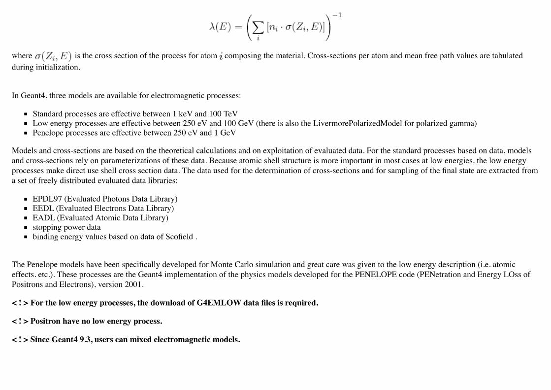
where is the cross section of the process for atom composing the material. Cross-sections per atom and mean free path values are tabulatedduring initialization.

In Geant4, three models are available for electromagnetic processes:

Standard processes are effective between 1 keV and 100 TeVLow energy processes are effective between 250 eV and 100 GeV (there is also the LivermorePolarizedModel for polarized gamma)Penelope processes are effective between 250 eV and 1 GeV

Models and cross-sections are based on the theoretical calculations and on exploitation of evaluated data. For the standard processes based on data, modelsand cross-sections rely on parameterizations of these data. Because atomic shell structure is more important in most cases at low energies, the low energyprocesses make direct use shell cross section data. The data used for the determination of cross-sections and for sampling of the final state are extracted froma set of freely distributed evaluated data libraries:

EPDL97 (Evaluated Photons Data Library)EEDL (Evaluated Electrons Data Library)EADL (Evaluated Atomic Data Library)stopping power databinding energy values based on data of Scofield .

The Penelope models have been specifically developed for Monte Carlo simulation and great care was given to the low energy description (i.e. atomiceffects, etc.). These processes are the Geant4 implementation of the physics models developed for the PENELOPE code (PENetration and Energy LOss ofPositrons and Electrons), version 2001.

< ! > For the low energy processes, the download of G4EMLOW data files is required.

< ! > Positron have no low energy process.

< ! > Since Geant4 9.3, users can mixed electromagnetic models.

Photoelectric effect

The photoelectric effect is the absorption of a photon by an atomic electon with the ejection of this electron from the atom. The energy of the outgoingelectron is:

where is the binding energy of the electron. Since a free electron cannot absorb a photon and also conserve momentum, the photoelectric effect alwaysoccurs on bound electrons while the nucleus absorbs the recoil momentum. The cross-section calculation is complex due to the combinaison of the electronDirac wave functions. It is simulated by using a parameterized photon absorption cross section to determine the mean free path, atomic shell data todetermine the energy of the ejected electron, and the K-shell angular distribution to sample the direction of the electron.

The cross-section depends on the atomic number of the material. The photoelectric process is favored by high materials. In the current implementationthe relaxation of the atom is not simulated, but instead is counted as a local energy deposit. For low energy process, the deexcitation of the atom is simulated.

To add photoelectric effect in GATE:

/gate/physics/addProcess PhotoElectric gamma

Note that the two following macro are equivalent because the default particle for the photoelectric process is the gamma only:

/gate/physics/addProcess PhotoElectric/gate/physics/addProcess PhotoElectric Default/gate/physics/addProcess PhotoElectric gamma

Then, choose the model:

/gate/physics/processes/PhotoElectric/setModel StandardModel

or

/gate/physics/processes/PhotoElectric/setModel LivermoreModel

or

/gate/physics/processes/PhotoElectric/setModel LivermorePolarizedModel

or

/gate/physics/processes/PhotoElectric/setModel PenelopeModel

Compton scattering

Compton process describes the photon scattering by free electrons. Although electrons are bound in matter, the electron can be considered as essentially freefor photons of energy much greater than the binding energy of the electron.

In the simulation, an empirical cross section formula is used, which reproduces the cross section data down to 10 keV. The final state is generated followingthe Klein-Nishina formula. For low energy incident photons, the simulation of the Compton scattering process is performed according to the same procedureused for the standard Compton scattering simulation, with the addition that Hubbel’s atomic form factor (or scattering function) is taken into account. Theangular and energy distribution of the incoherently scattered photon is then given by the product of the Klein-Nishina formula and the scattering function.

To add Compton scattering in GATE:

/gate/physics/addProcess Compton gamma

Note that the two following macro are equivalent because the defaut particle for the Compton process is only the gamma:

/gate/physics/addProcess Compton/gate/physics/addProcess Compton Default/gate/physics/addProcess Compton gamma

Then, choose the model :

/gate/physics/processes/Compton/setModel StandardModel

or

/gate/physics/processes/Compton/setModel LivermoreModel

or

/gate/physics/processes/Compton/setModel LivermorePolarizedModel

or

/gate/physics/processes/Compton/setModel PenelopeModel

Rayleigh scattering

Thomson and Rayleigh scattering are linked to Compton scattering. Thomson scattering is similer to Compton scattering in the classical limit i.e. thescattering of photons by free electrons. For Rayleigh scattering, all the electrons of the atom contribute in a coherent way (this process is also called coherentscattering).

For these processes, no energy is transferred to the target. The direction of the photon is the only modified parameter. Atoms are not excited or ionized. Athigh energies, the cross-sections of Thomson and Rayleigh scattering are very small and are neglected. For these reasons, the Rayleigh process is definedonly for low energy and Penelope models:

/gate/physics/addProcess RayleighScattering gamma/gate/physics/processes/RayleighScattering/setModel LivermoreModel /gate/physics/processes/RayleighScattering/setModel LivermorePolarizedModel/gate/physics/processes/RayleighScattering/setModel PenelopeModel

Pair production

The process of pair production describes the transformation of a photon into an electron-positron pair. In order to conserve momentum, this can only occur inthe presence of a third body, usually a nucleus. Moreover, the minimum energy required to create a pair is equal to the sum of the electron mass and positronmass (1.022 MeV).

To add pair production process in GATE:

/gate/physics/addProcess GammaConversion


/gate/physics/processes/GammaConversion/setModel StandardModel

or

/gate/physics/processes/GammaConversion/setModel LivermoreModel

or

/gate/physics/processes/GammaConversion/setModel LivermorePolarizedModel

or

/gate/physics/processes/GammaConversion/setModel PenelopeModel

Ionization

A charged particle passing through matter loses energy due to inelastic collision with atomic electrons of the material. Lost energy is transferred to the atomcausing ionization or excitation . The ionization energy loss is calculated using the Bethe-Bloch formula. The particle energy loss is divided intocontinuous energy loss and production of secondary electrons. The production threshold is defined as the minimum energy above which secondaryparticles will be produced and tracked. When , is included into the continuous energy loss and when > , secondary electrons areproduced. Energy loss due to excitation is included into continuous energy loss.

The mean excitation potential is the main parameter of the Bethe-Bloch formula. This quantity can be defined by user for each material (see chapter aboutgeometry and materials).

There are three processes to handle ionization:

for electron and positron

/gate/physics/addProcess ElectronIonisation e+/gate/physics/addProcess ElectronIonisation e-

for hadrons and ions

/gate/physics/addProcess HadronIonisation [Particle Name]

for ions

/gate/physics/addProcess IonIonisation [Particle Name]

The electron ionization process has three models available:

/gate/physics/processes/ElectronIonisation/setModel StandardModel e+/gate/physics/processes/ElectronIonisation/setModel StandardModel e-/gate/physics/processes/ElectronIonisation/setModel LivermoreModel e-/gate/physics/processes/ElectronIonisation/setModel PenelopeModel e+/gate/physics/processes/ElectronIonisation/setModel PenelopeModel e-

The new Geant4 model selection has not yet implemented for hadron ionization process in GATE V6.2. So users have to the old process/model selection.

The low energy model have a specific process for ionization of hadrons, ions, muons and taus:

/gate/physics/addProcess LowEnergyHadronIonisation

For the energy range between 1 keV and 2 MeV, this process has several models for the parametrization of electronic and nuclear stopping power:

/gate/physics/processes/LowEnergyHadronIonisation/setModel Elec_Ziegler1977p proton

Electronic stopping power models:

Elec_ICRU_R49p (default)Elec_ICRU_R49HeElec_Ziegler1977pElec_Ziegler1977HeElec_Ziegler1985pElec_SRIM2000p

Nuclear stopping power models:

Nuclear_ICRU_R49 (default)Nuclear_Ziegler1977Nuclear_Ziegler1985

It is possible to enable/disable nuclear stopping power for all hadrons and ions ionization processes:

/gate/physics/processes/[Process name]/setNuclearStoppingOn/gate/physics/processes/[Process name]/setNuclearStoppingOff

Example:

/gate/physics/processes/HadronIonisation/setNuclearStoppingOff

Bremsstrahlung

Bremsstrahlung process is the production of an electromagnetic radiation by a charged particle accelerated in the field of another charged particle, such as anucleus. The cross-section of bremsstrahlung is inversely proportional to the mass squared. Thus this process is more important for electron and positronthan other charge particles. As for ionization process, above a given threshold energy the energy loss is simulated by the explicit production of photons.Below the threshold, emission of soft photons is treated as a continuous energy loss. The bremsstrahlung energy spectrum is continuous.

/gate/physics/addProcess Bremsstrahlung e+/gate/physics/addProcess Bremsstrahlung e-

The electron ionization process has three models available:

/gate/physics/processes/Bremsstrahlung/setModel StandardModel e+/gate/physics/processes/Bremsstrahlung/setModel StandardModel e-/gate/physics/processes/Bremsstrahlung/setModel LivermoreModel e-/gate/physics/processes/Bremsstrahlung/setModel PenelopeModel e+/gate/physics/processes/Bremsstrahlung/setModel PenelopeModel e-

Positron and electron annihilation

In Geant4, the process which simulated the in-flight annihilation of a positron with an atomic electron is attached to positron. As is usually done in showerprograms, it is assumed here that the atomic electron is initially free and at rest. Also, annihilation processes producing one, or three or more, photons areignored because these processes are negligible compared to the annihilation into two photons.

/gate/physics/addProcess G4PositronAnnihilation e+


/gate/physics/processes/G4PositronAnnihilation/setModel StandardModel

or

/gate/physics/processes/G4PositronAnnihilation/setModel PenelopeModel

An improvement of the positron-electron annihilation has been developed to take into account the non-colinearity . The mean value of the angledistribution is (do not need model selection).

/gate/physics/addProcess PositronAnnihilation e+

Single and multiple Scattering

In addition to inelastic collisions with atomic electrons, charged particles passing through matter also suffer repeated elastic Coulomb scatterings fromnuclei. Elastic cross section is huge when particle energy decreases, so multiple scattering approach (MSC) should be introduced in order to have acceptableCPU performance of the simulation. The MSC model used in GEANT4 belongs to the class of condensed algorithm in which the global effects of thecollisions are simulated at the end of a track segment (step). The global effects generally computed in these codes are the net displacement, energy loss, andchange of direction of the charged particle. The model is based on Lewis' MSC theory and uses model functions to determine the angular and spatialdistributions after a step. The functions have been chosen in such a way as to give the same moments of the (angular and spatial) distributions as the Lewistheory. Two processes are available for multiple scattering. These processes are similar but they allow to define some sets of options for group of particles(electron/positron and hadron). The new Geant4 model selection has not yet implemented for multiple scattering process in GATE V6.2. So users have to theold process/model selection. The old MultipleScattering is now deprecated.

/gate/physics/addProcess eMultipleScattering e-/gate/physics/addProcess eMultipleScattering e+

/gate/physics/addProcess hMultipleScattering proton/gate/physics/addProcess hMultipleScattering alpha/gate/physics/addProcess hMultipleScattering GenericIon...

Single elastic scattering process is an alternative to the multiple scattering process. The advantage of the single scattering process is in possibility of usage oftheory based cross sections, in contrary to the Geant4 multiple scattering model, which uses a number of phenomenological approximations on top of Lewistheory. Because each of elastic collisions are simulated the simulation CPU time of charged particles significantly increasing in comparison with the multiplescattering approach.

/gate/physics/addProcess SingleScattering ...

Muon electromagnetic processes

Muons have their own electromagnetic processes:

Ionization

/gate/physics/addProcess MuIonisation mu+/gate/physics/addProcess MuIonisation mu-

Bremsstrahlung

/gate/physics/addProcess MuBremsstrahlung mu+/gate/physics/addProcess MuBremsstrahlung mu-

Direct production of (e+, e-) pairs by mu+ and mu-

/gate/physics/addProcess MuPairProduction mu+/gate/physics/addProcess MuPairProduction mu-

For ionization, the low energy model can handle muons.

Electromagnetic options

< ! > This part is recommanded for advanced users only!

< ! > Valid only from Geant4 version 9.2 - Gate V6.0 & V6.0.p01

< ! > In Geant4 version 9.2, options are available only for standard processes - Gate V6.0 & V6.0.p01

< ! > In case of using Gate V6.2, users must compile with Geant4 version 9.5 patch 01 - This Gate release is NOT compatible with previous Geant4version

Options are available for steering the standard electromagnetic processes. Some options modify all electromagnetic processes initialized in the simulation(Global options). Some options have to be defined for each processes.

Global options:

The following options manage the DEDX, mean free path and cross sections tables. User can defined the table range (default 0.1 keV - 100 TeV):

/gate/physics/setEMin 0.1 keV/gate/physics/setEMax 10 GeV

the number of bins of the DEDX table (default = 84):

/gate/physics/setDEDXBinning 500

and the number of bins of the mean free path table (default = 84):

/gate/physics/setLambdaBinning 500

Using cubic spline interpolation of DEDX and cross section tables, better interpolation was found to increase stability when varying transport parameters,such as cuts, of energy deposition of hadrons. Cubic spline interpolation is enabled by default. If the option was disable, the old linear interpolation is used:

/gate/physics/setSplineFlag true/gate/physics/setSplineFlag false

Step function

Continuous energy loss imposes a limit on the step size because of the energy dependence of the cross sections. It is generally assumed in MC programs thatthe particle cross sections are approximately constant along a step, i.e. the step size should be small enough that the change in cross section, from thebeginning of the step to the end, is also small. In principle one must use very small steps in order to insure an accurate simulation, however the computing

time increases as the step size decreases. A good compromise is to limit the step size by not allowing the stopping range of the particle to decrease by morethan a value [Ratio] during the step ([Ratio] = range/range). This condition works well for particles with kinetic energies > 1 MeV, but for lower energiesit gives very short step sizes.

To cure this problem a lower limit on the step size was introduced ([Final range]). The step size limit varies smoothly with decreasing energy from the value[Ratio] to the lowest possible value range cut [Final range]. By default for electron, [Ratio] = 0.2 and [Final range] = 0.1 mm.

/gate/physics/processes/[Process name]/SetStepFunction [Particle] [Ratio] [Final range] [Unit]

Parameter : [Particle]Parameter type : sOmittable : False

Parameter : [Ratio] (step/range)Parameter type : dOmittable : False

Parameter : [Final range]Parameter type : dOmittable : False

Parameter : [Unit]Parameter type : sOmittable : False

Example:

/gate/physics/processes/ElectronIonisation/setStepFunction e+ 0.01 1 mm

Linear loss limit

This cut is an other approach to limit the step size. In a step, the energy loss by a particle with a kinetic energy cannot exceed a value such as / < [Ratio]. By default for the ionization of an electron, the limit is 0.01.

/gate/physics/processes/IonIonisation/setLinearLossLimit [Particle] [Ratio]

Parameter : Particle or Group of particlesParameter type : sOmittable : False

Parameter : LimitParameter type : dOmittable : False

Example:

/gate/physics/processes/HadronIonisation/setLinearLossLimit proton 0.0001

Geometrical step limit type

This option allow to choose the transport algorithm for the multiple scattering process near to boundary. The two options proposed are safety anddistanceToBoundary. For instance, the distanceToBoundary algorithm limit the step size near to geometrical boundaries: only single scattering is appliedvery close to the boundaries.

/gate/physics/processes/MultipleScattering/setGeometricalStepLimiterType [Particle] [Limit type]

Parameter : Particle or Group of particlesParameter type : sOmittable : False

Parameter : Limit typeParameter type : sOmittable : False

Example:

/gate/physics/processes/MultipleScattering/setGeometricalStepLimiterType proton distanceToBoundary

Hadronic processes

Hadronic processes described the interactions between incident hadrons/ions and the target nuclei. We also include decays of hadron and nuclei in this part.There is no strict frontier between nucleon-nucleon collision processes but we can distinguish four main process types in function of the energy and theimpact parameter. At low energies, collisions lead to incomplete fusion in central collisions and to elastic scattering or inelastic scattering in peripherical

collisions. At higher energies, there is fragmentation into several lighter fragments or nucleons for central collisions and into participant and the spectatorregions for peripherical collisions. In Geant4, fusion, inelastic scattering and fragmentation processed are included in the inelastic process type. Inelasticprocesses had three main steps:

cascade: the incident particle interacts strongly with the target and produces secondary particlespreequilibrium (thermalization process): the excited target nucleus switches into equilibrated state by emitting excitons and light nuclei.de-excitation: the equilibrated nuclear residues evaporates into nucleons/light nuclei or breaks up into several fragments.

Each hadronic process may have one or more data sets associated with it. The term "data set" is meant, in a broad sense, to be an object that encapsulatesmethods and data for calculating total cross sections for a given process. The methods and data may take many forms, from a simple equation using a fewhard-wired numbers to a sophisticated parameterization using large data tables. For the evaluation of cross sections, the list has a LIFO (Last In First Out)priority, meaning that data sets added later to the list will have priority over those added earlier to the list.

The final state is produced using models coupled to processes. In Geant4, any model can be run together with any other model and the ranges of applicabilityfor the different models can be steered. This way, highly specialized models (valid only for one material and particle, and applicable only in a very restrictedenergy range) can be used in the same application, together with more general code, in a coherent fashion. Each model has an intrinsic range of applicability,and the model chosen for a simulation depends very much on the use-case. Three types of hadronic models have been implemented: parametrization drivenmodels, data driven models, and theory driven models.

Most of hadronic processes need an explicit choice of models while a lots of processes have a default data set.

Main Geant4 models

LHEP

LHEP is the model used by default. It is based on code GHEISHA developed since 1978 by H. Fesefeldt to simulate hadron-nucleus interactions. The lowenergy part is valid from few hundred MeV to 20 GeV. The model is based on the principle of the intranuclear cascade and only the first hadron-nucleusinteraction is simulated in detail. Other interactions in the nucleus are simulated by generating additional hadrons, simply treated as secondary particles canthemselves generate their own intranuclear cascade. LHEP is a fully parameterized model but the physical meaning of the large number of adjustableparameters is sometimes unclear. Its main assets are the broad energy range covered, good reproduction of average values of distributions and computationtimes.

Example: G4LCapture, G4LENeutronInelastic, G4LFission, G4LCapture, G4LEProtonInelastic, G4LEPionMinusInelastic, G4LEPionPlusInelastic...

Bertini cascade

The intranuclear cascade model of Bertini has been developed by H W. Bertini in 1963. This code includes the intranuclear cascade model of Bertini, a pre-equilibrium model, a simple model of nucleus explosion, a model of fission and evaporation model.

Binary cascade

The Geant4 Binary Cascade is an intranuclear cascade propagating primary and secondary particles in a nucleus. The energy range and type of projectilecovered are the same as Bertini model. From a theoretical point of view, this model is much more evolved taking into account a large number of resonancesand fully modeled in three dimensions. Interactions are between a primary or secondary particle and an individual nucleon of the nucleus, leading to thename Binary Cascade. Cross section data are used to select collisions. Where available, experimental cross sections are used by the simulation. Propagatingof particles is the nuclear field is done by numerically solving the equation of motion. The cascade terminates when the average and maximum energy ofsecondaries is below threshold. The remaining fragments are treated by precompound and de-excitation models.

QMD

Pre compound

Elastic scattering

In elastic scattering, the projectile and the target particles do not changed during the collision and no other particles are produced. Two processes areavailable for hadrons and ions. The first one is the old elastic process.

/gate/physics/addProcess HadronElastic Default/gate/physics/processes/HadronElastic/setModel G4LElastic Default

or

/gate/physics/addProcess HadronElastic /gate/physics/processes/HadronElastic/setModel G4LElastic

or

/gate/physics/addProcess HadronElastic proton/gate/physics/processes/HadronElastic/setModel G4LElastic proton/gate/physics/addProcess HadronElastic alpha

/gate/physics/processes/HadronElastic/setModel G4LElastic alpha.........

This process has a default dataset (G4HadronElasticDataSet) and 6 models

G4LElasticG4NeutronHPElasticG4NeutronHPorLElasticG4ElasticHadrNucleusHEG4LEppG4LEnp

The alternative process is an improvement of the first process. It is supposed to be a good mix between the models of the fist process:

/gate/physics/addProcess HadronElastic/gate/physics/processes/HadronElastic/setModel G4HadronElastic/gate/physics/processes/HadronElastic/setDataSet G4HadronElasticDataSet

For this process, there is only one model and a main dataset (G4HadronElasticDataSet). An other dataset for low energy neutrons is also available(G4NeutronHPElasticData).

Inelastic process for proton

This process manage inelastic interaction of proton with matter. For example, the selection of two models with energy range for proton inelastic process (theonly default particle is the proton):

/gate/physics/addProcess ProtonInelastic/gate/physics/processes/ProtonInelastic/setModel G4BinaryCascade/gate/physics/processes/ProtonInelastic/G4BinaryCascade/setEmin 170 MeV/gate/physics/processes/ProtonInelastic/G4BinaryCascade/setEmax 500 GeV/gate/physics/processes/ProtonInelastic/setModel PreCompound/gate/physics/processes/ProtonInelastic/PreCompound/setEmin 0 MeV/gate/physics/processes/ProtonInelastic/PreCompound/setEmax 170 MeV

This process has a default dataset (G4HadronInelasticDataSet) and an alternative dataset (G4ProtonInelasticCrossSection). There are 6 models available:

G4LEProtonInelastic

G4BertiniCascadeG4BinaryCascadePreCompoundG4QMDReaction

Inelastic process for ion

This process manage inelastic interaction of ions with matter. This process is valid for GenericIon, alpha, deuteron and triton. For example, a completeselection of models and data set for ions:

/gate/physics/addProcess IonInelastic Default/gate/physics/processes/IonInelastic/setModel G4BinaryLightIonReaction Default/gate/physics/processes/IonInelastic/setModel G4LEDeuteronInelastic deuteron/gate/physics/processes/IonInelastic/setModel G4LETritonInelastic triton/gate/physics/processes/IonInelastic/setModel G4LEAlphaInelastic alpha/gate/physics/processes/IonInelastic/G4BinaryLightIonReaction/setEmin 80 MeV deuteron/gate/physics/processes/IonInelastic/G4BinaryLightIonReaction/setEmax 20 GeV deuteron/gate/physics/processes/IonInelastic/G4BinaryLightIonReaction/setEmin 80 MeV triton/gate/physics/processes/IonInelastic/G4BinaryLightIonReaction/setEmax 20 GeV triton/gate/physics/processes/IonInelastic/G4BinaryLightIonReaction/setEmin 80 MeV alpha/gate/physics/processes/IonInelastic/G4BinaryLightIonReaction/setEmax 20 GeV alpha/gate/physics/processes/IonInelastic/G4LEDeuteronInelastic/setEmin 0 MeV deuteron/gate/physics/processes/IonInelastic/G4LEDeuteronInelastic/setEmax 80 MeV deuteron/gate/physics/processes/IonInelastic/G4LETritonInelastic/setEmin 0 MeV triton/gate/physics/processes/IonInelastic/G4LETritonInelastic/setEmax 80 MeV triton/gate/physics/processes/IonInelastic/G4LEAlphaInelastic/setEmin 0 MeV alpha/gate/physics/processes/IonInelastic/G4LEAlphaInelastic/setEmax 80 MeV alpha/gate/physics/processes/IonInelastic/setDataSet G4IonsShenCrossSection GenericIon/gate/physics/processes/IonInelastic/setDataSet G4TripathiLightCrossSection deuteron/gate/physics/processes/IonInelastic/setDataSet G4TripathiLightCrossSection triton/gate/physics/processes/IonInelastic/setDataSet G4TripathiLightCrossSection alpha

The IonInelastic process includes the G4IonInelasticProcess for GenericIon, the G4DeuteronInelasticProcess for deuteron, the G4TritonInelasticProcess fortriton and the G4AlphaInelasticProcess for alpha. The G4QMDReaction model and the G4BinaryLightIonReaction model are available for all ions. ForGenericIon, one additional model (G4BinaryLightIonReaction) and 5 datasets are available :

G4TripathiCrossSectionG4IonsKoxCrossSectionG4IonsShenCrossSectionG4IonsSihverCrossSectionG4TripathiLightCrossSection

Alpha, deuteron and triton have a default data set (G4HadronInelasticDataSet) and a alternative dataset (G4TripathiLightCrossSection). There are alsospecific models for each particle: G4LEDeuteronInelastic, G4LETritonInelastic, G4LEAlphaInelastic.

Pions

The inelastic interaction of pi+ and pi- with matter is handled by PionPlusInelastic and PionMinusInelastic processes. These processes have two specificmodels (G4LEPionMinusInelastic - G4LEPionPlusInelastic) and three common models:

Bertini CascadeBinary CascadeLeading Particle Bias

The default dataset is G4HadronInelasticDataSet. There is an alternative dataset: G4PiNuclearCrossSection.

/gate/physics/addProcess PionPlusInelastic pi+/gate/physics/processes/PionPlusInelastic/setModel G4LEPionPlusInelastic pi+/gate/physics/addProcess PionMinusInelastic pi-/gate/physics/processes/PionMinusInelastic/setModel G4LEPionMinusInelastic pi-

Neutrons

The interactions of neutrons at low energies are split into four parts. We consider radiative capture, elastic scattering, fission, and inelastic scattering asseparate processes. Each processes have standard models and datasets like others particles. In additions, some "high precision" models and datasets areprovided for low energy interactions. The high precision neutron models depend on an evaluated neutron data library (G4NDL) for cross sections, angulardistributions and final state information. G4NDL data comes largely from the ENDF/B-VI library.

< ! > For the low energy processes, the download of G4NDL data files is required.

Radiative Capture

The G4LCapture model generates the final state for neutron capture. The G4NeutronHPCapture model generates the final state for neutron capture using thehigh precision neutron model. The G4NeutronHPorLCapture model generates the final state for neutron capture using the high precision neutron modelwhen sufficient high precision data is available for the selected element or isotope. When there is insufficient data, the neutron is captured using the lessprecise Low Energy Parameterized model.

The G4HadronCaptureDataSet is the default dataset for this process. The alternative high precision dataset is G4NeutronHPCaptureData.

/gate/physics/addProcess NeutronCapture/gate/physics/processes/NeutronCapture/setModel G4LCapture

Inelastic scattering

The G4NeutronInelasticProcess is similar than proton inelastic and ion inelastic processes. In addtion to the standard models (G4LENeutronInelastic,G4BertiniCascade, G4BinaryCascade, PreCompound, LeadingParticleBias), two models using the high precision data are available. TheG4NeutronHPInelastic model generates the final state for inelastic neutron scattering. The G4NeutronHPorLEInelastic model generates the final state forinelastic neutron scattering using the high precision neutron model when sufficient high precision data is available for the selected element or isotope. Whenthere is insufficient data, the neutron is scattered inelastically using the less precise Low Energy Parameterized model (G4LENeutronInelastic).

The G4HadronInelasticDataSet is the default dataset for this process. An alternative dataset is the G4NeutronInelasticCrossSection. The high precisiondataset is G4NeutronHPInelasticData.

/gate/physics/addProcess NeutronInelastic/gate/physics/processes/NeutronInelastic/setModel PreCompound

Fission

The G4LFission model generates the final state for fission. The G4NeutronHPFission model generates the final state for neutron-induced fission using thehigh precision neutron model. The G4NeutronHPorLFission model generates the final state for neutron-induced fission using the high precision neutronmodel when sufficient high precision data is available for the selected element or isotope. When there is insufficient data, neutron-induced fission isperformed using the less precise Low Energy Parameterized model.

The G4HadronFissionDataSet is the default dataset for this process. The alternative high precision dataset is G4NeutronHPFissionData.

/gate/physics/addProcess Fission/gate/physics/processes/Fission/setModel G4LFission

Particle decay

Particle decay is the spontaneous process of one elementary particle transforming into other elementary particles. If the particles created are not stable, thedecay process can continue. The majority of decays in Geant4 are implemented using the G4PhaseSpaceDecayChannel class. It simulates phase spacedecays with isotropic angular distributions in the center-of-mass system.

/gate/physics/addProcess Decay

Radioactive decay

Radioactive decay is the process in which an unstable atomic nucleus spontaneously loses energy by emitting ionizing particles and radiation. In Geant4, thedecay of radioactive nuclei by , , and emission and by electron capture are taken into account. The simulation model is empirical and data-driven,and uses the Evaluated Nuclear Structure Data File (ENSDF).

< ! > The download of radioactive decay data files is required.

/gate/physics/addProcess RadioactiveDecay

Optical physics processes

For detailed information, see Users Guide V8.0:Generating and tracking optical photons.

Bulk Absorption

This process kills the optical photon. It requires the Material properties filled by the user with the Absorption length (average distance traveled by a photonbefore being absorbed by the medium).

/gate/physics/addProcess OpticalAbsorption

Rayleigh Scattering

This process depends on the particle’s polarization. A photon which is not assigned a polarization at production may not be Rayleigh scattered. The photon isscattered in a new direction that is required to be perpendicular to the photon’s new polarization in such a way that the final direction, initial and finalpolarizations are all in one plane. The process requires the Material properties filled with Rayleigh scattering length (average distance traveled by a photonbefore it is Rayleigh scattered in the medium).

N.B: For Water ONLY, when scattering lengths are not specified but the user, the Geant4 code calculates them following the Einstein-Smoluchowskiformula.

/gate/physics/addProcess OpticalRayleigh

Mie Scattering

Mie Scattering is an analytical solution of Maxwell’s equations for scattering of optical photons by spherical particles. It is significant only when the radiusof the scattering object is of order of the wave length.The analytical expressions for Mie Scattering are very complicated since they are a series sum ofBessel functions.One common approximation made is call Henyey-Greenstein (HG). The implementation in GATE (Geant4) follows the HG approximationand the treatment of polarization and momentum are similar to that of Rayleigh scattering.

The process requires Material properties to be filled by the user with Mie scattering length data (MIEHG). In practice, the user not only needs to provide theattenuation length of Mie scattering, but also needs to provide the constant parameters of the approximation: MIEHG_FORWARD, MIEHG_BACKWARD,and MIEHG_FORWARD_RATIO.

/gate/physics/addProcess OpticalMie

Processes at Boundaries

The optical boundary process design relies on the concept of surfaces: physical properties of the surface itself (stored in Materials.xml) and characteristics ofthe surface specifying the two ordered pairs of physical volumes touching at the surface (Surface.xml).

When the surface concept is not needed, and a perfectly smooth surface exists between two dielectric materials, the only relevant property is the index ofrefraction, a quantity stored with the material.

/gate/physics/addProcess OpticalBoundary

Wavelength Shifting or Fluorescence

Fluorescence is the result of a three-stage process that occurs in certain molecules called fluorophores or fluorescent dyes. A fluorescent probe is afluorophore designed to respond to a specific stimulus or to localize within a specific region of a biological specimen. The process responsible for thefluorescence involves the creation of an excited electronic singlet state by optical absorption and subsequent emission of an optical photon of lower energythan the excitation photon.

/gate/physics/addProcess OpticalWLS

Magnetic fieldA magnetic field can be defined. It will be attached and thus active in the whole world volume. It is currently not possible to confine the field to anothervolume. The following command can be used to activate and define the magnetic field properties:

/gate/geometry/setMagField Bx By Bz Unit

Here is the help for the command:

Command /gate/geometry/setMagFieldGuidance :Define magnetic field.

Parameter : Bx Parameter type : d Omittable : False

Parameter : By Parameter type : d Omittable : False

Parameter : Bz Parameter type : d Omittable : False

Parameter : Unit Parameter type : s Omittable : True Default value : tesla Candidates : T kG G tesla kilogauss gauss

Retrieved from "http://wiki.opengatecollaboration.org/index.php?title=Users_Guide_V8.0:Setting_up_the_physics&oldid=914"


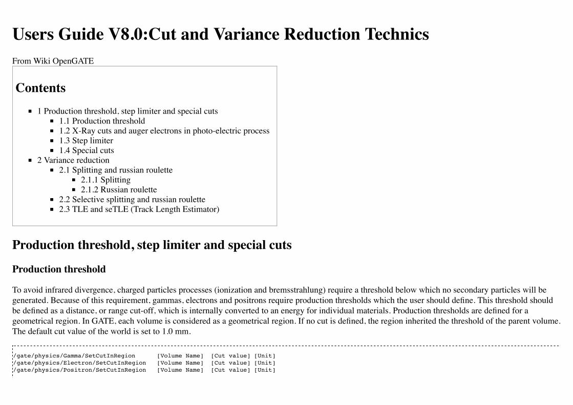
Users Guide V8.0:Cut and Variance Reduction TechnicsFrom Wiki OpenGATE

Contents1 Production threshold, step limiter and special cuts

1.1 Production threshold1.2 X-Ray cuts and auger electrons in photo-electric process1.3 Step limiter1.4 Special cuts

2 Variance reduction2.1 Splitting and russian roulette

2.1.1 Splitting2.1.2 Russian roulette

2.2 Selective splitting and russian roulette2.3 TLE and seTLE (Track Length Estimator)

Production threshold, step limiter and special cuts

Production threshold

To avoid infrared divergence, charged particles processes (ionization and bremsstrahlung) require a threshold below which no secondary particles will begenerated. Because of this requirement, gammas, electrons and positrons require production thresholds which the user should define. This threshold shouldbe defined as a distance, or range cut-off, which is internally converted to an energy for individual materials. Production thresholds are defined for ageometrical region. In GATE, each volume is considered as a geometrical region. If no cut is defined, the region inherited the threshold of the parent volume.The default cut value of the world is set to 1.0 mm.

/gate/physics/Gamma/SetCutInRegion [Volume Name] [Cut value] [Unit] /gate/physics/Electron/SetCutInRegion [Volume Name] [Cut value] [Unit]/gate/physics/Positron/SetCutInRegion [Volume Name] [Cut value] [Unit]

For example:

/gate/physics/Gamma/SetCutInRegion world 1.0 mm

The list of production threshold in range and in energy for each volume can be display with the command:

/gate/physics/displayCuts

User should use this command after the initilization.

X-Ray cuts and auger electrons in photo-electric process

Secondary electron and photon production in low energy photo-electric process (livermore and penelope models) could be customized.

The auger electron could be activated in livermore and penelope models:

/gate/physics/processes/PhotoElectric/setAugerElectron true

In livermore model, an energy threshold could be defined from which secondary particles are produced. The threshold is defined for the whole world of thesimulation.

/gate/physics/processes/PhotoElectric/setDeltaRayCut [value] [unit]/gate/physics/processes/PhotoElectric/setXRayCut [value] [unit]

Step limiter

< ! > This part is recommended for advanced users only!

The step limiter can be considered as a process with fixed step size. It allows to limit the maximum size of step. As for production threshold, the step limiteris defined for a geometrical region and the region can inherit the step limiter of the parent volume. User have to define the step size in the region:

/gate/physics/SetMaxStepSizeInRegion [Volume Name] [Step size] [Unit]

For example:

/gate/physics/SetMaxStepSizeInRegion world 1.0 mm

Then, the step limiter process has to be add to particles:

/gate/physics/ActivateStepLimiter proton

Special cuts

< ! > This part is recommended for advanced users only!

The user can define four cuts to limit the tracking of a particle:

the maximum total track lengththe maximum total time of flightthe minimum kinetic energythe minimum remaining range

While step limiter is affected to a step, special cuts are affected to a track. When a particle is stopped, the energy is deposited locally. As for productionthreshold, the special cuts are defined for a geometrical region and the region can inherit the special cuts of the parent volume.

User have to define the values of the special cuts in the region and activate the cuts for particles.

/gate/physics/SetMaxToFInRegion world 5 s/gate/physics/SetMinKineticEnergyInRegion world 1 keV/gate/physics/SetMaxTrackLengthInRegion world 0.01 mm/gate/physics/SetMinRemainingRangeInRegion world 0.02 mm/gate/physics/ActivateSpecialCuts proton

The user does not have to define all the cuts. The ActivateSpecialCuts command is effective for all the special cuts that are defined.

Variance reductionTwo standard reduction variance techniques are available in GATE: splitting and russian roulette. The weight of secondary particles is recalculated infunction of the number of secondaries generated. User can also defined filters to increase the efficiency of these techniques.

< ! > User have to verify that all the tools he used in his simulation take into account particle weight!

Splitting and russian roulette

Splitting

In this technique, the final state of the process is generated N times and the weight of each secondary is 1/N.

/gate/physics/processes/Bremsstrahlung/activateSplitting [Particle] [N]


Parameter : [N]Parameter type : iOmittable : False

Example: to split 100 times the electron bremsstrahlung photon (not that we specify that the e- is the particle which do the bremsstrahlung, but the split isapplied on the generated photon):

/gate/physics/processes/Bremsstrahlung/activateSplitting e- 100

Russian roulette

In this technique, Russian roulette is played on secondary particles. The survival probability is 1/N and the weight of each secondary is N.

/gate/physics/processes/Bremsstrahlung/activateRussianRoulette [Particle] [N]


Parameter : [N]Parameter type : iOmittable : False

Example: to keep 2% of electron bremsstrahlung photon (2/100 = 1/50):

/gate/physics/processes/Bremsstrahlung/activateRussianRoulette e- 50

Selective splitting and russian roulette

To increase the efficiency of the splitting and the russian roulette technique, user can add selections criteria on the incident (primary) or secondary particles.The selection is done with filters. The filters for splitting and russian roulette are the same as for Actors. For example, to split bremsstrahlung photons with avector direction inside a cone of 20 degrees around the x axis:

/gate/physics/processes/Bremsstrahlung/addFilter angleFilter secondaries/gate/physics/processes/Bremsstrahlung/secondaries/angleFilter/setAngle 20/gate/physics/processes/Bremsstrahlung/secondaries/angleFilter/setDirection 1 0 0

There are several filters types: filters on particle, particle ID, energy, direction, volume... See the chapter on Actor for a description of all filters.

TLE and seTLE (Track Length Estimator)

See the TLEDoseActor and SETLEDoseActor here.

Retrieved from "http://wiki.opengatecollaboration.org/index.php?title=Users_Guide_V8.0:Cut_and_Variance_Reduction_Technics&oldid=915"


Users Guide V8.0:SourceFrom Wiki OpenGATE

To introduce a source into a GATE simulation, the user has to define the type of source (voxelized, linacBeam, phaseSpace, PencilBeam, TPSPencilBeam orGPS) and its feature (angle, energy, and position). Many activity distributions are available in GATE. At each new event, the source manager decidesrandomly which source decays, and generates for it one or more primary particles.

Contents1 Creating a source

1.1 Adding a source1.2 Defining the type of source1.3 Defining the energy1.4 Defining the angular distribution of the emission1.5 Defining the shape of the source1.6 Define the placement of the source1.7 Movement of a source

1.7.1 Attach to a volume1.7.2 Confining a source1.7.3 Example: two gammas

1.8 Defining a cold source1.9 Visualizing a source1.10 Intensity

2 Pencil Beam source3 TPS Pencil Beam source4 The fastY90 source

Creating a source

Different type of sources can be defined in the same GATE simulation. Each source is independent. The command to create a source is given below:

/gate/source/NAME

where "NAME" defines the name of the source.

Adding a source

The next step is to add the source. For this, user has to type the following GATE command:

/gate/source/addSource NAME

or

/gate/source/addSource NAME gps

In this example, a source "NAME" is added. Once a source has been added, a series of properties must be assigned to it. These properties are: activity, typeof particle(s), energy distribution, energy value or bounds, angular emission, spatial distribution and location, and half-life. The commands required to assignthese properties are described in the following paragraphs.

Defining the type of source

Ion source

The ion source type can simulate any ion by defining its atomic number (Z), atomic weight (A), ionic charge in units of energy (Q), and its excitation energyin keV (E). It incorporates both the radioactive decay and the atomic de-excitation. This is the most "realistic" way of simulating a radionuclide; however, itis also the slowest.

To use the ion source:

/gate/source/NAME/gps/particle ion/gate/source/NAME/gps/ion 8 15 0 0 /gate/source/NAME/setForcedUnstableFlag true/gate/source/NAME/useDefaultHalfLife

In the above example, an ion source of oxygen-15 has been defined with Z=8, A=15, Q=0, E=0 . If it is too slow, other options are available, as describedbelow.

Simple particles

You can choose from a long list of simple particles , gamma, etc) to use in your simulations (use the help command to obtain the full list). Forexample:

/gate/source/NAME/gps/particle gamma

defines a photon source and

/gate/source/NAME/gps/particle e+

defines a positron source. If you choose to use a particle, you will have to define more properties. As an example, the correct use of a positron sourcesimulating fluorine-18 is:

/gate/source/NAME/gps/particle e+/gate/source/NAME/gps/energytype Fluor18/gate/source/NAME/setForcedUnstableFlag true/gate/source/NAME/setForcedHalfLife 6586 s

In the above example, more properties of fluorine-18 have been added by using the helper keyword Fluor18 (see below): half-life and energy distribution.Note that the branching ratios are not respected with this kind of simulation because no decay is simulated, i.e. emission is 100% positron. You may want tolower the activity by an appropriate factor to take this better point into account.

Helper keywords

These keywords are defined to help you to define the particle properties. The first three keywords define an positron energy distribution resulting fromcommon beta emitters, and the last one defines a special two-particle source. For instance, Fluor18 defines the positron energy spectrum of fluorine-18. Note that this keyword define only the energy spectrum, you still have to specifythe particle and the half-life.

Back-to-back This keyword is implemented for PET simulations where two annihilation photons are generated at 180 degrees. This type of source is fasterto simulate than the ion source or the positron source and allows for selecting emission angle. To use the back-to-back source type:

/gate/source/NAME/setType backtoback

Note that there are no radioactive decays simulated when using the back-to-back type and that you still have to define the particle (gamma), energy type(Mono) and energy-value (0.511 MeV).

FastI124

FastI124 is a special source implementing a simplified decay scheme of the non-pure beta emitter iodine-124 in which positrons are emitted but notneutrinos, there is no nuclear recoil, gammas are emitted if their emission probability is > 1%; and no atomic de-excitation occurs (no x-rays, Augerelectrons). These simplifications allow for an increase in speed with respect to the ion source while retaining important features of iodine-124, i.e. gammasmay be emitted concurrently with positrons to possibly create "dirty" coincidences. Since decay is simulated, branching ratios are respected hence no activitycompensation is necessary.

To use the fastI124 source:

/gate/source/NAME/setType fastI124

The source takes care of particle definitions (gamma, positron) and energy distribution so that there is no need to specify a particle or mention its energy.

Defining the activity

To define the activity of the given source, the user defines the amount of activity and its unit using the following command:

/gate/source/NAME/setActivity 5. becquerel

In this example, the total activity of the source referred to as "NAME" is set to 5 Bq. The activity can be defined in Curie (Ci) as well as in Becquerel (Bq).

Defining the energy

Energy distribution

If the source does not take care of the type of energy distribution (e.g. fastI124), then it has to be explicitly defined. This can be achieved either by using apre-defined spectrum (see helper keywords above) or by using built-in distributions.

Candidates for built-in energy distributions are: mono-energetic "Mono", linear "Lin", powerlaw "Pow", exponential "Exp", Gaussian "Gauss",bremstrahlung "Brem", black-body "Bbody", cosmic diffuse gamma ray "Cdg", user-defined histogram "UserSpectrum", arbitrary point-wise spectrum"Arb", and user-defined energy per nucleon histogram "Epn". Capitalization is important: only strings given exactly as above will be recognized.

In the following example, all particles have the same energy:

/gate/source/NAME/gps/energytype Mono

Energy value

You may have to specify the energy value (or bounds) depending on the type of energy distribution you have selected. For example, for monoenergeticdistributions (like back-to-back sources), you specify the energy value with:

/gate/source/NAME/gps/monoenergy 511. keV

In the case of ions, the kinetic energy must be 0 since the ions are at rest:

/gate/source/NAME/gps/monoenergy 0. ev

Any type of energy unit within the International System of Units (SI) can be used: eV, GeV, MeV, keV...

Examples

1. ion source for fluorine-18

/gate/source/NAME/gps/particle ion /gate/source/NAME/gps/ion 9 18 0 0 /gate/source/NAME/gps/monoenergy 0. keV /gate/source/NAME/setForcedUnstableFlag true# WARNING - DEBUG - New command line to debug the use of ion particle type

/gate/source/F18/useDefaultHalfLife

2. positron source for flourine-18

/gate/source/NAME/gps/particle e+ /gate/source/NAME/gps/energytype Fluor18 /gate/source/NAME/setForcedUnstableFlag true /gate/source/NAME/setForcedHalfLife 6586 s

3. backtoback for fluorine-18

/gate/source/NAME/setType backtoback /gate/source/NAME/gps/particle gamma /gate/source/NAME/gps/monoenergy 511. keV /gate/source/NAME/setForcedUnstableFlag true /gate/source/NAME/setForcedHalfLife 6586 s

4. fast iodine-124 source

/gate/source/NAME/setType fastI124 /gate/source/NAME/setForcedUnstableFlag true /gate/source/NAME/setForcedHalfLife 360806 s

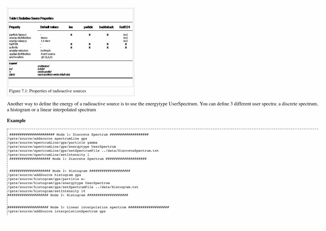
Figure 7.1: Properties of radioactive sources

Another way to define the energy of a radioactive source is to use the energytype UserSpectrum. You can define 3 different user spectra: a discrete spectrum,a histogram or a linear interpolated spectrum

Example

###################### Mode 1: Discrete Spectrum ###################/gate/source/addsource spectrumLine gps/gate/source/spectrumLine/gps/particle gamma/gate/source/spectrumLine/gps/energytype UserSpectrum/gate/source/spectrumLine/gps/setSpectrumFile ../data/DiscreteSpectrum.txt/gate/source/spectrumLine/setIntensity 1 #################### Mode 1: Discrete Spectrum #################### #################### Mode 2: Histogram ####################/gate/source/addSource histogram gps/gate/source/histogram/gps/particle e-/gate/source/histogram/gps/energytype UserSpectrum/gate/source/histogram/gps/setSpectrumFile ../data/Histogram.txt/gate/source/histogram/setIntensity 10#################### Mode 2: Histogram ####################

#################### Mode 3: Linear interpolation spectrum ####################/gate/source/addSource interpolationSpectrum gps

/gate/source/interpolationSpectrum/gps/particle e-/gate/source/interpolationSpectrum/gps/energytype UserSpectrum/gate/source/interpolationSpectrum/gps/setSpectrumFile ../data/InterpolationSpectrum.txt /gate/source/interpolationSpectrum/setIntensity 10#################### Mode 3: Linear interpolation spectrum ####################

The user spectra are specified by a text file. The first number on the first line indicates the mode as follows: 1 - discrete, 2 - histogram, and 3 - interpolatedspectrum. The second number on the first line specifies the energy, in MeV, of the lower edge of the first bin in histogram mode. (Though ignored in thediscrete and interpolated modes, it must be present for the file to parse correctly.) The remaining lines specify the energy, in MeV, and the associatedprobability weighting. The probabilities will normalized by the GATE software.

The discrete spectrum generates particles with one of the listed energies.

################DiscreteSpectrum.txt ###################1 00.2 0.20.4 0.40.6 0.60.8 0.81.0 1.01.2 0.81.4 0.61.6 0.41.8 0.2###################################################

In histogram mode, the energy specified on each line corresponds to the upper edge of the respective bin. The energies of the generated particles will bebetween the minimum energy, specified on the first line of the file, and the upper edge of the last bin. Within each bin, the energies are distributed uniformly.

################## Histogram.txt #####################2 22.2 0.22.4 0.42.6 0.62.8 0.83.0 13.2 0.83.4 0.63.6 0.43.8 0.2##################################################

In interpolated mode, the energy of the generated particle will fall between the first and last energy specified, according to the probability distribution createdby piecewise-linear interpolation between the points provided.

################ InterpolationSpectrum.txt #############3 04.2 0.24.4 0.44.6 0.64.8 0.85.0 15.2 0.85.4 0.65.6 0.45.8 0.2#################################################

The following image present the result obtain for the 3 examples (available in example_UserSpectrum repository)

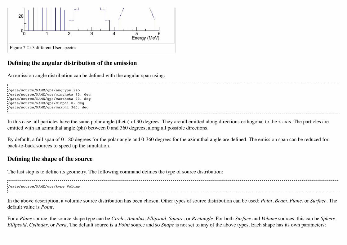
Figure 7.2 : 3 different User spectra

Defining the angular distribution of the emission

An emission angle distribution can be defined with the angular span using:

/gate/source/NAME/gps/angtype iso /gate/source/NAME/gps/mintheta 90. deg /gate/source/NAME/gps/maxtheta 90. deg /gate/source/NAME/gps/minphi 0. deg /gate/source/NAME/gps/maxphi 360. deg

In this case, all particles have the same polar angle (theta) of 90 degrees. They are all emitted along directions orthogonal to the z-axis. The particles areemitted with an azimuthal angle (phi) between 0 and 360 degrees, along all possible directions.

By default, a full span of 0-180 degrees for the polar angle and 0-360 degrees for the azimuthal angle are defined. The emission span can be reduced forback-to-back sources to speed up the simulation.

Defining the shape of the source

The last step is to define its geometry. The following command defines the type of source distribution:

/gate/source/NAME/gps/type Volume

In the above description, a volumic source distribution has been chosen. Other types of source distribution can be used: Point, Beam, Plane, or Surface. Thedefault value is Point.

For a Plane source, the source shape type can be Circle, Annulus, Ellipsoid, Square, or Rectangle. For both Surface and Volume sources, this can be Sphere,Ellipsoid, Cylinder, or Para. The default source is a Point source and so Shape is not set to any of the above types. Each shape has its own parameters:

/gate/source/NAME/gps/shape Cylinder /gate/source/NAME/gps/radius 1. cm /gate/source/NAME/gps/halfz 1. mm

In the previous commands, the source is a cylinder with a radius of 1 cm and a length of 2 mm. Very often, the half-length is given rather than the full length.

To define a circle, the radius (radius) should be set. (In reality it is not really a circle but a disk).To define an annulus, the inner (radius0) and outer radii (radius) should be given.To define an ellipse, square , or rectangle, the half-lengths along x (halfx) and y (halfy) have to be given.To define a sphere, only the radius (radius) only has to be specified.To define an ellipsoid, its half-lenghths in x (halfx), y (halfy), and z (halfz) have to be given.To define a cylinder with its axis along the z-axis, only the radius (radius) and the z half-length (halfz) have to be specified.To define parallelepipeds, the x (halfx), y (halfy), and z (halfz) half-lengths, and the angles alpha (paralp), theta (parthe), and phi (parphi) have to begiven.

Define the placement of the source

The position of the source distribution can be defined using:

/gate/source/NAME/gps/centre 1. 0. 0. cm

In that example, the centre of the source distribution is 1 cm off-centered along the x-axis.

Movement of a source

Attach to a volume

The source can be attached to a volume:

/gate/source/[Source name]/attachTo [Volume Name]

If the volume moves during the simulation, the source moves along with the volume. Note that when attaching a source to a volume, the source's placementbecomes relative to the volume.

Confining a source

Note: this is the old way of moving a source. It is very inefficient. Please consider using the "Attach to a volume" method instead.

To define sources in movement, the source distribution have to be confined in a Geant4 volume. This volume will be animated using the usual GATEcommand as described in Chapter 4 of this manual.

The command:

/gate/source/NAME/gps/confine NAME_P

specifies that the emission must be confined to a volume of the Geant4 geometry. In this case, the emission distribution is the intersection of the GeneralParticle Source (GPS) and the Geant4 volume. The Geant4 volume must be specified by its physical volume name: GATEname + '_P'.

One should note that the confinment slows down the simulation, the confinement volume must have an intersection with the GPS shape, and the confinementvolume must not be too large as compared to the GPS shape.

A complete example of a moving source can be found in the SPECT benchmark or in the macro hereafter:

# Define the shape/dimensions of the moving source /gate/MovingSource/geometry/setRmax 5. cm /gate/MovingSource/geometry/setRmin 0. cm /gate/MovingSource/geometry/setHeight 20. cm /gate/MovingSource/moves/insert translation /gate/MovingSource/translation/setSpeed 0 0 0.04 cm/s

# Define the shape/dimensions of the large sourcecontainer # that should contain the full trajectory of the moving source /gate/source/SourceContainer/gps/type Volume /gate/source/SourceContainer/gps/shape Cylinder /gate/source/SourceContainer/gps/radius 4. cm /gate/source/SourceContainer/gps/halfz 30. cm # Define the placement of the SourceContainer /gate/source/SourceContainer/gps/centre 0. 0. 0. cm

# Define the source as a gamma source /gate/source/SourceContainer/gps/particle gamma # Define the gamma energy /gate/source/SourceContainer/gps/energy 140. keV # Set the activity of the source /gate/source/SourceContainer/setActivity 5000. Bq # Define a confinement and confine the large container to# the MovingSource at a position defined by the time and # the translation speed /gate/source/SourceContainer/gps/confine MovingSource_P

Example: two gammas

The following example gives a script to insert a point source of back-to-back type.

# A new source with an arbitrary name #(``twogamma) is created /gate/source/addSource twogamma # The total activity of the source is set /gate/source/twogamma/setActivity 0.0000001 Ci # The source emits pairs of particles back-to-back /gate/source/twogamma/setType backtoback # The particles emitted by the source are gammas /gate/source/twogamma/gps/particle gamma # The gammas have an energy of 511 keV /gate/source/twogamma/gps/energytype Mono /gate/source/twogamma/gps/monoenergy 0.511 MeV # The source is a full sphere with radius 0.1 mm, # located at the centre of the FOV /gate/source/twogamma/gps/type Volume /gate/source/twogamma/gps/shape Sphere /gate/source/twogamma/gps/radius 0.1 mm /gate/source/twogamma/gps/centre 0. 0. 0. cm # The angular distribution of emission angles is isotropic /gate/source/twogamma/gps/angtype iso # The parameters below mean that the source emits # at all angles along the z axis /gate/source/twogamma/gps/mintheta 0. deg /gate/source/twogamma/gps/maxtheta 180. deg # Uncomment the parameters below if you want the source # to emit in an XY (transverse) plane /gate/source/twogamma/gps/mintheta 90. deg /gate/source/twogamma/gps/maxtheta 90. deg # The parameters below mean that the source emits # at all angles in the transverse (XY) directions /gate/source/twogamma/gps/minphi 0. deg /gate/source/twogamma/gps/maxphi 360. deg

Defining a cold source

To define a cold (i.e. with no activity) volume in a phantom, a dedicated command is available.

The command:

/gate/source/NAME/gps/Forbid Volume_Name

The following example explains how to use this option. First you must define a volume that defines the cold region:

/gate/world/daughters/name cold_area /gate/world/daughters/insert cylinder /gate/cold_area/vis/forceWireframe /gate/cold_area/vis/setColor green /gate/cold_area/geometry/setRmax 3.0 cm /gate/cold_area/geometry/setHeight 1. cm

Then you describe your source with the Forbid command:

/gate/source/addSource number1 /gate/source/number1/setActivity 100000. becquerel /gate/source/number1/gps/particle gamma /gate/source/number1/setType backtoback /gate/source/number1/gps/type Volume /gate/source/number1/gps/shape Cylinder /gate/source/number1/gps/radius 5. cm /gate/source/number1/gps/halfz 0.5 cm /gate/source/number1/gps/centre 0. 0. 0. cm /gate/source/number1/gps/monoenergy 511. keV /gate/source/number1/gps/angtype iso /gate/source/number1/gps/Forbid cold_area /gate/source/number1/dump 1 /gate/source/list

It is important to remember that the /gate/run/initialize command must have been executed prior to using the Forbid command because phantom geometriesare not available until after they are initialized.

Visualizing a source

To check that sources are at the right location in the geometry, you can use the following command

/gate/source/[Source name]/visualize

along with a real time viewer (e.g. OpenGL). To visualize a source, Gate will randomly pick a certain number of points within the source and display themon the screen, along with the geometry. The full syntax is:

/gate/source/[Source name]/visualize count color size

where name is the name of the source, count is the number of random points to pick up (must be > 0 and <= 10000), color is the color to assign to thosepoints (valid colors are: white, gray, grey, black, red, green, blue, cyan, magenta, yellow), and size is the screen size (in pixels) of each point (must be > 0and <= 20 ).

Depending on the size and shape of the source, more or fewer points may be necessary.

Example:

/gate/source/backgroundSource/visualize 2000 yellow 3 /gate/source/hotRegion/visualize 5000 red 2

Intensity

If several sources have been added and no activity is defined, user can use intensity to define the source priorities. A high intensity correspond to a highpriority. For each event, the source is randomly selected taking into account the intensity of each sources.

/gate/source/MyBeam/setIntensity [value]

Pencil Beam sourceThe simulation source can be a pencil beam. This source allows for characterizing a beam of particles having energy and optical properties. This beam canbe used for instance in order to characterize a clinical beam interacting in a passive beam line or to characterize a specific spot from an active beam scanningdelivery system.

/gate/source/addSource [Source name] PencilBeam

One can select the type of particle used for the pencil beam (proton, e-, etc.):

/gate/source/ [Source name] /setParticleType [particle_type]

Alternatively, one can define a specific type of ion, by defining the particle type as "GenericIon" and then specifying the particle parameters of the ion to begenerated: Z: AtomicNumber, A: AtomicMass, Q: Charge of Ion (in unit of e), E: Excitation energy (in keV). As an example, the definition of a C12 ionbeam is given:

/gate/source/ [Source name] /setParticleType GenericIon/gate/source/PBS/setIonProperties 6 12 6 0

The energy spectrum of the source is Gaussian and is defined by a mean energy and standard deviation:

/gate/source/ [Source name] /setEnergy [mean_energy] [Unit]/gate/source/ [Source name] /setSigmaEnergy [energy_standard_deviation] [Unit]

The source position can be set as follows:

/gate/source/ [Source name] /setPosition [Pos_X Pos_Y Pos_Z] [Unit]

The pencil beam shape is Gaussian. The spot size can is defined by the standard deviation of the normal probability density function in x and y directions.The beam default direction being +z.

/gate/source/ [Source name] /setSigmaX [spot_size_X] [Unit]

/gate/source/ [Source name] /setSigmaY [spot_size_Y] [Unit]

The beam is also characterized by its divergences: Theta in the XoZ plan and Phi in the YoZ plan. The beam divergence is defined by the standard deviationof the normal probability density function:

/gate/source/ [Source name] /setSigmaTheta [divergence_Theta] [Unit]/gate/source/ [Source name] /setSigmaPhi [divergence_Phi] [Unit]

The correlation between spot size and divergence (in the two plans) is characterized by the beam emittance. The beam emittance is defined by the standarddeviation of the normal probability density function. The Emittance of the beam has to be lower (or equal) than the ellipse phase space area:[Emittance_X_Theta] <= Pi* [divergence_Theta] * [spot_size_X] and [Emittance_Y_Phi] <= Pi* [divergence_Phi] * [spot_size_Y].

Please note that for emittance, the unit cannot be selected and has to be "mm*mrad".

/gate/source/ [Source name] /setEllipseXThetaEmittance [Emittance_X_Theta] mm*mrad/gate/source/ [Source name] /setEllipseYPhiEmittance [Emittance_Y_Phi] mm*mrad

When defining the beam parameters, one can define the beam convergence or divergence in the two plans (XoZ and YoZ), by setting the "RotationNorm"either to "positive" for a convergent beam or to "negative" for a divergent beam.

/gate/source/ [Source name] /setEllipseXThetaRotationNorm [negative or positive]/gate/source/ [Source name] /setEllipseYPhiRotationNorm [negative or positive]

Users can also define the direction of the beam, which is by default +z (0 0 1), by rotating the beam along the x, y and z axis. For instance, to rotate the beamdirection around the x-axis by 90°.

/gate/source/ [Source name] /setRotationAxis 1 0 0/gate/source/ [Source name] /setRotationAngle 90 deg

The number of particles simulated is defined using the conventional command:

/gate/application/setTotalNumberOfPrimaries [number_of_primaries]

Example

In the following example, we defined a 180 MeV proton beam, with 1 MeV energy spread. The beam is asymmetrical and convergent. The direction is -Y.

/gate/source/addSource PBS PencilBeam/gate/source/PBS/setParticleType proton/gate/source/PBS/setEnergy 188.0 MeV/gate/source/PBS/setSigmaEnergy 1.0 MeV/gate/source/PBS/setPosition 0 0 0 mm/gate/source/PBS/setSigmaX 2 mm/gate/source/PBS/setSigmaY 4 mm/gate/source/PBS/setSigmaTheta 3.3 mrad/gate/source/PBS/setSigmaPhi 3.8 mrad/gate/source/PBS/setEllipseXThetaEmittance 15 mm*mrad/gate/source/PBS/setEllipseXThetaRotationNorm negative/gate/source/PBS/setEllipseYPhiEmittance 20 mm*mrad/gate/source/PBS/setEllipseYPhiRotationNorm negative/gate/source/PBS/setRotationAxis 1 0 0/gate/source/PBS/setRotationAngle 90 deg/gate/application/setTotalNumberOfPrimaries 10

TPS Pencil Beam sourceThe source of the simulation can be a stack of pencil beams. This source has been designed in order to allow the simulation of real treatment plans for activebeam scanning delivery techniques.

/gate/source/addSource [Source name] TPSPencilBeam

One can select the type of particle used for the pencil beam (proton, e-, etc.):

/gate/source/ [Source name] /setParticleType [particle_type]

A treatment plan is made of one or multiple fields, each field being described by a gantry angle and a collection of pencil beams having different energies,directions, weights etc. user has to select the "plan description file" of the simulation:

/gate/source/ [Source name] /setPlan [plan_description_file]

It is possible to simulate all fields simultaneously or only some of them, by setting the "NotAllowedField" option. This option allows for ignoring specificfields:

/gate/source/ [Source name] /setNotAllowedFieldID [field_ID_1]/gate/source/ [Source name] /setNotAllowedFieldID [field_ID_2]/gate/source/ [Source name] /setNotAllowedFieldID [field_ID_3]

etc.

In the "plan description file", each single spot is characterized by its position at treatment isocenter and also by its weight (intensity). By default, the weightcorresponds to the number of Monitor Units (MU) delivered and is converted into a number of particles according to the proton stopping power in air.Warning! The conversion of MU to number of particles has been developed for protons only ! However, it is possible to define the particle weight as anumber of particles (and not as MU), by setting the following command to true:

/gate/source/ [Source name] /setSpotIntensityAsNbProtons true

As each spot has an intensity in the treatment plan, it is possible to simulate either each spot with the same probability and setting the dose scoring weightequal to the intensity, or simulate each spot with a probability related to the intensity and setting the dose scoring weight to 1. The second option is stronglyadvised (for efficiency) and used by default. It is possible to select the first or second option by setting the "FlatGenerationFlag" to true or false, respectively.

/gate/source/ [Source name] /setFlatGenerationFlag false

The physical properties of each single pencil beam delivered are computed using the "source description file". This file consists in a set of polynomialequations allowing to define the physical and optical properties of each single pencil beam with energy. Pencil beam properties are those described in theprevious section "Pencil Beam source":

/gate/source/ [Source name] /setSourceDescriptionFile [source_description_file]

Irradiation systems can be tuned with either a convergent beam or a divergent beam at the delivery system exit. By default, the system is defined asdivergent. User can define either a convergent or a divergent beam by setting the following command either to "true" or "false", respectively:

/gate/source/ [Source name] /setBeamConvergence [true or false]

The number of particles simulated is defined using the conventional command

/gate/application/setTotalNumberOfPrimaries 10

Example

The following example shows how to simulate a proton treatment plan based on the 2 following input files: "MyPlanDescriptionFile.txt" and"MySourceDescriptionFile.txt". The beam is considered convergent and the spot intensities are defined as number of protons.

/gate/source/addSource PBS TPSPencilBeam/gate/source/PBS/setParticleType proton/gate/source/PBS/setPlan MyPlanDescriptionFile.txt/gate/source/PBS/setNotAllowedFieldID 1/gate/source/PBS/setFlatGenerationFlag false/gate/source/PBS/setSourceDescriptionFile MySourceDescriptionFile.txt/gate/source/PBS/setSpotIntensityAsNbProtons true/gate/source/PBS/setBeamConvergence true/gate/application/setTotalNumberOfPrimaries 10

About the "source_description_file" It contains the source to isocenter distance, and scanning magnets distance to isocenter in x- and y-directions. Theseparameters allow for computing the position and direction of each single pencil beam at the nozzle exit. It contains also 8 polynomial equations: 2 describingthe energy properties (mean energy in MeV and energy spread in % of the mean energy) and 6 describing the optical properties of the beam (spot size inmm, beam divergence in rad and beam emittance in mm.rad, in x- and y-directions at nozzle exit). Polynomials are functions of the system energy, which isread in the "plan description file" for each pencil beam. For each polynomial, one has to give the polynomial order and then the polynomial parameters. Forinstance, for a second order polynomial (ax² + bx + c), one has to give the polynomial order: 2, followed by the a, b and c parameters in this order. Pleasenote that their is no choice about the units used for the different polynomials!! Please have a look to example "example_Radiotherapy/example5" in thesource code.

About the "plan_description_file" It contains many informations about the plan, but not all of them are taken into account for the simulation, as forinstance the number of fractions. These additional informations may be used in further releases. Please have a look to example"example_Radiotherapy/example5" and "Gate/examples/example_Radiotherapy/example5/data/PlanDescriptionToGATE.txt" file. Warning, the unused fieldsof the plan description file cannot be removed. The main parameters of the file are the number of fields, gantry angle for each field, energy of each layer fromeach field, number of spot in each layer, spot description (position in x- and y- direction at isocenter and intensity) for each spot from each layer.

The fastY90 source

The fastY90 source will be part of GATE release 8.0, but it is also available in the development versions of GATE 7.2 availiable on GitHub as of June 2016

The fastY90 source can be used to simulate PET or SPECT imaging of 90Y sources. Rather than simulating the full electron transport of the emitted betaparticle, the fastY90 source uses a pre-calculated bremsstrahlung kernel to generate the photons directly to speed up the simulation. Note that since the kernelhas been calculated using a point source in water, simulations that use this source are only valid for modelling sources inside water or materials of similardensity and Zeff. For accurate simulation, the attenuating media must also extend somewhat beyond the range of the source by several mm. Although the sizeof the pre-calculated kernel has a radius of 12 mm, more than 95% of all bremsstrahlung is generated within 6 mm of the source, a higher fraction if only thehigher energy bremsstrahlung is considered.

The fastY90 model includes the positron arising from internal pair production (0+/0+ transition), though not the 2.186 MeV gamma (2+/0+ transition).

To use the fastY90 source:

/gate/source/addSource mySource fastY90

Simuations with the fastY90 source can be further sped up by adding a low energy cutoff to the bremsstrahlung generation, effictively ignoring thosebremsstrahlung photons with too little energy to play any role in imaging. For example:

/gate/source/mySource/setMinBremEnergy 50 keV

The 90Y decay produces a positron with a prevalence of about 31.86 ppm. Although the model defaults to this value, it can be modified (for testing purposes,for example) by the setPositronProbabiliity command:

/gate/source/mySource/setPositronProbability 0.00003186

Using a voxelized distribution with the fastY90 source

The fastY90 source can be used with a voxelized distribution. The voxelized distribution must be in the Interfile format, with a header file that contains, atminimum, the name of the data file, the matrix size, and the scale factor.

/gate/source/mySource/loadVoxelizedPhantom tia_map.h.hdr

!INTERFILE :=!name of data file :=tia_map.vmatrix size[1] := 256matrix size[2] := 256matrix size[3] := 147scale factor (mm/pixel) [1]:= 1.91scale factor (mm/pixel) [2]:= -1.91scale factor (mm/pixel) [3]:= -2.00

The data file must be a raw binary containing data in IEEE 32-bit floating point format. The voxelized distribution will be scaled internally to create a 3Dprobability map of the geometry of the source, but the total activity is set by the setActivity command as for any other source. By default, the location of thevoxelized source will be centred at the origin. The position of the voxelized distribution can also be changed using the setVoxelizedPhantomPositioncommand to specify the position of the first pixel in the data file.

gate/source/mySource/setVoxelizedPhantomPosition -3.5 6.0 -10.0 cm

Retrieved from "http://wiki.opengatecollaboration.org/index.php?title=Users_Guide_V8.0:Source&oldid=1000"


Users Guide V8.0:Voxelized Source and PhantomFrom Wiki OpenGATE

Contents1 Introduction2 Voxelized phantoms

2.1 Description of voxelized geometry2.1.1 Regular parameterization method2.1.2 Nested parameterization method2.1.3 Regionalized parameterization method2.1.4 Fictitious interaction

2.2 Description of voxelized phantoms2.2.1 Conversion into material definitions

2.2.1.1 Range translator2.2.1.2 Units to materials conversion descriptor

2.2.2 Example of voxelized phantom description macro2.2.3 For RT applications only: Automated HU stoichiometric calibration

3 Voxelized sources3.1 Conversion into activity values3.2 Example of voxelized source description macro

4 Dose collection5 Real-time motion management for voxellized source and phantom6 Examples

IntroductionVoxelized source and phantom's purpose is the use of digital phantoms or patient data as inhomogeneous anthropomorphic attenuation maps or emissionsources so as to simulate and thus reproduce realistic acquisitions.

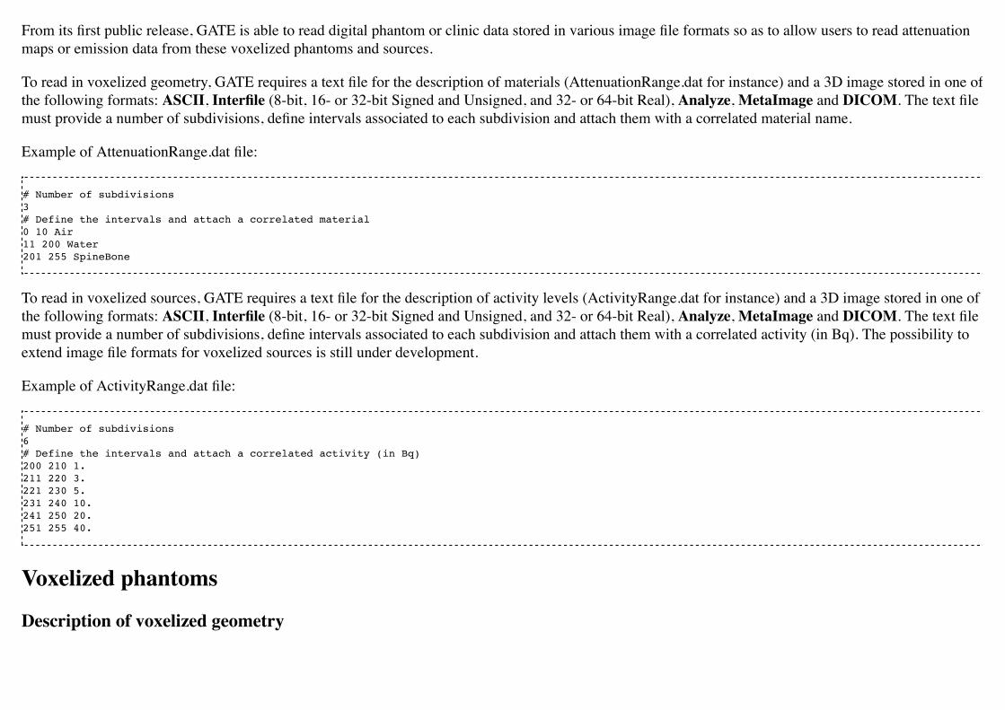
From its first public release, GATE is able to read digital phantom or clinic data stored in various image file formats so as to allow users to read attenuationmaps or emission data from these voxelized phantoms and sources.

To read in voxelized geometry, GATE requires a text file for the description of materials (AttenuationRange.dat for instance) and a 3D image stored in one ofthe following formats: ASCII, Interfile (8-bit, 16- or 32-bit Signed and Unsigned, and 32- or 64-bit Real), Analyze, MetaImage and DICOM. The text filemust provide a number of subdivisions, define intervals associated to each subdivision and attach them with a correlated material name.

Example of AttenuationRange.dat file:

# Number of subdivisions3# Define the intervals and attach a correlated material0 10 Air11 200 Water201 255 SpineBone

To read in voxelized sources, GATE requires a text file for the description of activity levels (ActivityRange.dat for instance) and a 3D image stored in one ofthe following formats: ASCII, Interfile (8-bit, 16- or 32-bit Signed and Unsigned, and 32- or 64-bit Real), Analyze, MetaImage and DICOM. The text filemust provide a number of subdivisions, define intervals associated to each subdivision and attach them with a correlated activity (in Bq). The possibility toextend image file formats for voxelized sources is still under development.

Example of ActivityRange.dat file:

# Number of subdivisions6# Define the intervals and attach a correlated activity (in Bq)200 210 1.211 220 3.221 230 5.231 240 10.241 250 20.251 255 40.

Voxelized phantoms

Description of voxelized geometry

To import digital phantom or patient data to voxelized geometry, GATE needs a convenient method to describe multiple copies of a volume inside a mothervolume. Obviously, this description can lead to problem of memory consumption and hence affect the efficiency of tracking algorithm (computation of thedistance to the next boundary, search for the neighbouring voxels, particles stopped at each boundary etc.)

To save both memory consumption and computation time when simulating voxelized phantoms, new parameterization methods derived from Geant4together with their corresponding navigation algorithms are often developed.

Regular parameterization method

Since Geant4.9.1 a new navigation algorithm, dubbed regular navigation, can be used for the tracking of particles in voxelized volumes. The regularnavigation algorithm performs fast direct neighbouring voxel identification without a large memory overhead. This is the major source of acceleration of theimplemented regular navigation algorithm. In addition, boundaries between voxels which share the same material can be ignored. Using this option, thegeometry only limits tracking at the boundary between voxels with different materials, providing a significant reduction of the number of propagation steps.The regular navigator uses a new algorithm that performs this search only for the neighbours of the actual voxel. It therefore highly reduces the time spenton this search, as much as the number of voxels is large. It also includes a new method called ComputeStepSkippingEqualMaterials; when a boundary isencountered, the navigator searches for the next voxel it should enter and check if its material is the same as the actual one. If this is the case, this method isdirectly called again without passing through the navigator manager which loads the new properties of the next voxel, etc. Therefore the fewer the materials,the faster the simulation. In conclusion, the time saved using the regular navigator is directly dependent on the number of voxels and the number of differentmaterials contained in the voxelized phantom. The better acceleration factors were obtained while simulating PET acquisitions (3 different materials: air,water, bone) with finely sampled phantom definitions. This factor could be around 3 in those cases. However in any case, even with a lot of differentmaterials, this navigator will always be faster than using older navigators such as parameterizedBoxMatrix or compressedMatrix. That is the reason whythese navigators still be progressively deprecated.

Additionally, as the SkipEqualMaterials method can lead to fewer G4steps, one may want to force the stepping process at each boundary. In that case, themethod can be inactivated using the following command:

/gate/world/anyname/setSkipEqualMaterials 0

Also the particle tracking will inevitably be less effective.

Nested parameterization method

Another method of creating parametrized volumes in Geant4, using nested parametrization and the corresponding navigation algorithm has been available inGATE since version 6.1. Based on parametrized approach, this method allows GATE storing a single voxel representation in memory and dynamicallychanging its location and composition at run-time during the navigation. The main advantage of this method is high efficiency in memory space. Whilereusing the same mechanism as parameterized volume, Nested representation also splits the 3D volume along the three principal directions, allowinglogarithmic finding of neighbouring voxels. Nested approach supposes geometry has three-dimensional regular reputation of same shape and size of volumeswithout gap between volumes and material of such volumes are changing according to the position. Instead of direct three-dimensional parameterizedvolume, one can use replicas for the first and second axes sequentially, and then use one-dimensional parameterization along the third axis. This approachrequires much less memory access and consumption for geometry optimization and gives much faster navigation for ultra-large number of voxels. UsingNested representation, images are split into sub-volumes of homogeneous composition, which are parallelepipeds, either of the voxel size or larger. The maindrawback is that all the particles are forced to stop at the boundaries of all parallelepipeds, generating a supplementary step and additional time cost, even ifthe two neighboring parallelepipeds share the same content. Such artificial steps occur very often as human organs are far from being parallelepipedic.

Regionalized parameterization method

Recently, some GATE developers have proposed a new method for efficient particle transportation in voxelized geometry for Monte Carlo simulations,especially for calculating dose distribution in CT images for radiation therapy. The proposed approach, based on an implicit volume representation namedsegmented volume, coupled with an adapted segmentation procedure and a distance map, allows them to minimize the number of boundary crossings, whichslows down simulation. Before being implemented within GATE, the method was developed using the GEANT4 toolkit and compared to four othermethods: one box per voxel, parameterized volumes, octree-based volumes, and nested parameterized volumes. For each representation, they compared dosedistribution, time, and memory consumption. The proposed method allows them to decrease computational time by up to a factor of 15, while keepingmemory consumption low, and without any modification of the transportation engine. Speeding up is related to the geometry complexity and the number ofdifferent materials used. They obtained an optimal number of steps with removal of all unnecessary steps between adjacent voxels sharing a similar material.However, the cost of each step is increased. When the number of steps cannot be decreased enough, due for example, to the large number of materialboundaries, such a method is not considered suitable. Thus, optimizing the representation of an image in memory potentially increases computing efficiency.

Fictitious interaction

Important note: so far, this method is available in GATE v7.0 version using Interfile reader only.

For detailed information, please refer to Users Guide V8.0:Voxelized_Source_and_Phantom#Speeding-up_tracking:_Fictitious_interaction

Description of voxelized phantoms

Regular, Nested and Regionalized parametrization methods together with their corresponding navigation algorithms are available in GATE V7.0 forvoxelized phantoms. Note that so far their current implementations do not support voxel visualization attributes on a per material basis.

To create a parameterized phantom object using any of the three above-mentioned methods, one can use the corresponding command lines as follows:

/gate/world/daughters/name anyname /gate/world/daughters/insert ImageRegularParametrisedVolume

Or

/gate/world/daughters/name anyname /gate/world/daughters/insert ImageNestedParametrisedVolume

Or

/gate/world/daughters/name anyname /gate/world/daughters/insert ImageRegionalizedVolume

All these three methods supports 3D images stored in various image file formats, which is automatically defined from their extension:

ASCIIInterfile format: header .h33 + raw image .i33Analyze format: header .hdr + raw image .imgMetaImage format: header. mhd + raw image .rawDICOM format: a series of .dcm files

Conversion into material definitions

Whatever the navigation algorithm selected, conversion of image grayscales into material definitions is performed as follows:

When already defined in GateMaterials.db file, appropriate material properties are assigned to each voxel encoded value using either a range translator (to beused with images providing label values) or a units to materials conversion descriptor (to be used with images providing label or HU values).

Range translator

Tables read by the range translator have a prescribed format.

The first line defines the number of material subdivisions (i.e. the number of subsequent lines). The following lines describe the intervals (i.e. range) ofencoded values (bits or segmented values) associated to each subdivision (i.e material), followed by a material name. A particular material will be assignedto each voxel whose value falls within the material range.

One can keep specifying visibility boolean (true or false) and color attribute values (red, green, blue components and transparency coefficient) within therange translator as he did when using a previous GATE version. However, as previously mentioned, so far current implementations of any of the three newparametrization methods do not support voxel visualization attributes on a per material basis, hence preventing the voxelized phantom from being displayed.

Example of a range translation table (AttenuationRange.dat, for instance)

4 0 0 Air false 0.0 0.0 0.0 0.24 4 Water true 1.0 0.0 1.0 0.25 5 Water true 0.0 1.0 0.0 0.26 15 SpineBone true 0.0 0.0 1.0 0.2

In this example, the number of material subdivisions is 4. Material Air is assigned to pixels with value 0, Water to pixels with value 4 and 5, and SpineBoneto pixels with value between 6 and 15.

Units to materials conversion descriptor

Units to materials conversion descriptor is a simple text file with three columns: Label or HU_start, Label or HU_end and material_name. It allows toassociate a material to each label or HU voxel encoded value in the image. This text file can be written by hand or generated with the automated method,especially for HU values (see Users_Guide_V8.0:Voxelized_Source_and_Phantom#For_RT_applications_only:_Automated_HU_stoichiometric_calibrationsection)

Example of a units to materials conversion descriptor (AttenuationRange.dat, for instance)

6 0 1 Air1 4 Water4 6 Bone6 16 SpineBone

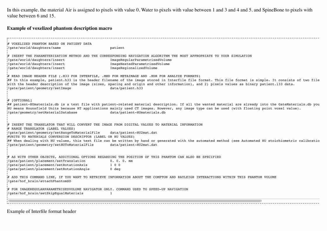
In this example, the material Air is assigned to pixels with value 0, Water to pixels with value between 1 and 3 and 4 and 5, and SpineBone to pixels withvalue between 6 and 15.

Example of voxelized phantom description macro

# VOXELIZED PHANTOM BASED ON PATIENT DATA/gate/world/daughters/name patient

# INSERT THE PARAMETERIZATION METHOD AND THE CORRESPONDING NAVIGATION ALGORITHM THE MOST APPROPRIATE TO YOUR SIMULATION/gate/world/daughters/insert ImageRegularParametrisedVolume/gate/world/daughters/insert ImageNestedParametrisedVolume/gate/world/daughters/insert ImageRegionalizedVolume

# READ IMAGE HEADER FILE (.H33 FOR INTERFILE, .MHD FOR METAIMAGE AND .HDR FOR ANALYZE FORMATS)## In this example, patient.h33 is the header filename of the image stored in Interfile file format. This file format is simple. It consists of two files: 1) patient.h33 is a ASCII filewith the header description of the image (sizes, spacing and origin and other information), and 2) pixels values as binary patient.i33 data. /gate/patient/geometry/setImage data/patient.h33

# [OPTIONAL]## patient-HUmaterials.db is a text file with patient-related material description. If all the wanted material are already into the GateMaterials.db you do not need such additional file.HU means Hounsfield Units because RT applications mainly used CT images. However, any image type can be used (with floating point voxel value). /gate/geometry/setMaterialDatabase data/patient-HUmaterials.db

# INSERT THE TRANSLATOR THAT WILL CONVERT THE IMAGE FROM DIGITAL VALUES TO MATERIAL INFORMATION# RANGE TRANSLATOR (LABEL VALUES)/gate/patient/geometry/setRangeToMaterialFile data/patient-HU2mat.dat#UNITS TO MATERIALS CONVERSION DESCRIPTOR (LABEL OR HU VALUES)## When dealing with HU values, this text file can be written by hand or generated with the automated method (see Automated HU stoichiometric calibration). /gate/patient/geometry/setHUToMaterialFile data/patient-HU2mat.dat

# AS WITH OTHER OBJECTS, ADDITIONAL OPTIONS REGARDING THE POSITION OF THIS PHANTOM CAN ALSO BE SPECIFIED/gate/patient/placement/setTranslation 0. 0. 0. mm/gate/patient/placement/setRotationAxis 1 0 0/gate/patient/placement/setRotationAngle 0 deg

# ADD THIS COMMAND LINE, IF YOU WANT TO RETRIEVE INFORMATION ABOUT THE COMPTON AND RAYLEIGH INTERACTIONS WITHIN THIS PHANTOM VOLUME/gate/hof_brain/attachPhantomSD

# FOR IMAGEREGULARPARAMETRISEDVOLUME NAVIGATOR ONLY. COMMAND USED TO SPEED-UP NAVIGATION/gate/hof_brain/setSkipEqualMaterials 1

Example of Interfile format header

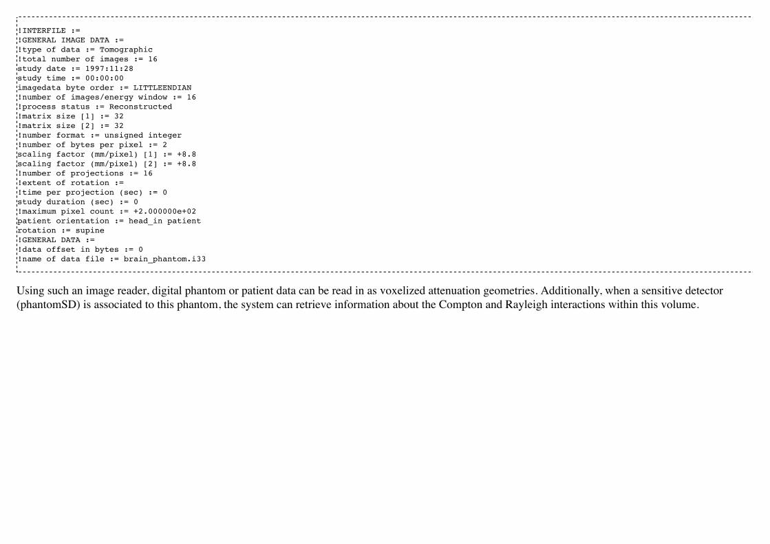
!INTERFILE := !GENERAL IMAGE DATA := !type of data := Tomographic !total number of images := 16 study date := 1997:11:28 study time := 00:00:00 imagedata byte order := LITTLEENDIAN !number of images/energy window := 16 !process status := Reconstructed !matrix size [1] := 32 !matrix size [2] := 32 !number format := unsigned integer !number of bytes per pixel := 2 scaling factor (mm/pixel) [1] := +8.8scaling factor (mm/pixel) [2] := +8.8 !number of projections := 16 !extent of rotation := !time per projection (sec) := 0 study duration (sec) := 0 !maximum pixel count := +2.000000e+02 patient orientation := head_in patientrotation := supine !GENERAL DATA := !data offset in bytes := 0 !name of data file := brain_phantom.i33

Using such an image reader, digital phantom or patient data can be read in as voxelized attenuation geometries. Additionally, when a sensitive detector(phantomSD) is associated to this phantom, the system can retrieve information about the Compton and Rayleigh interactions within this volume.

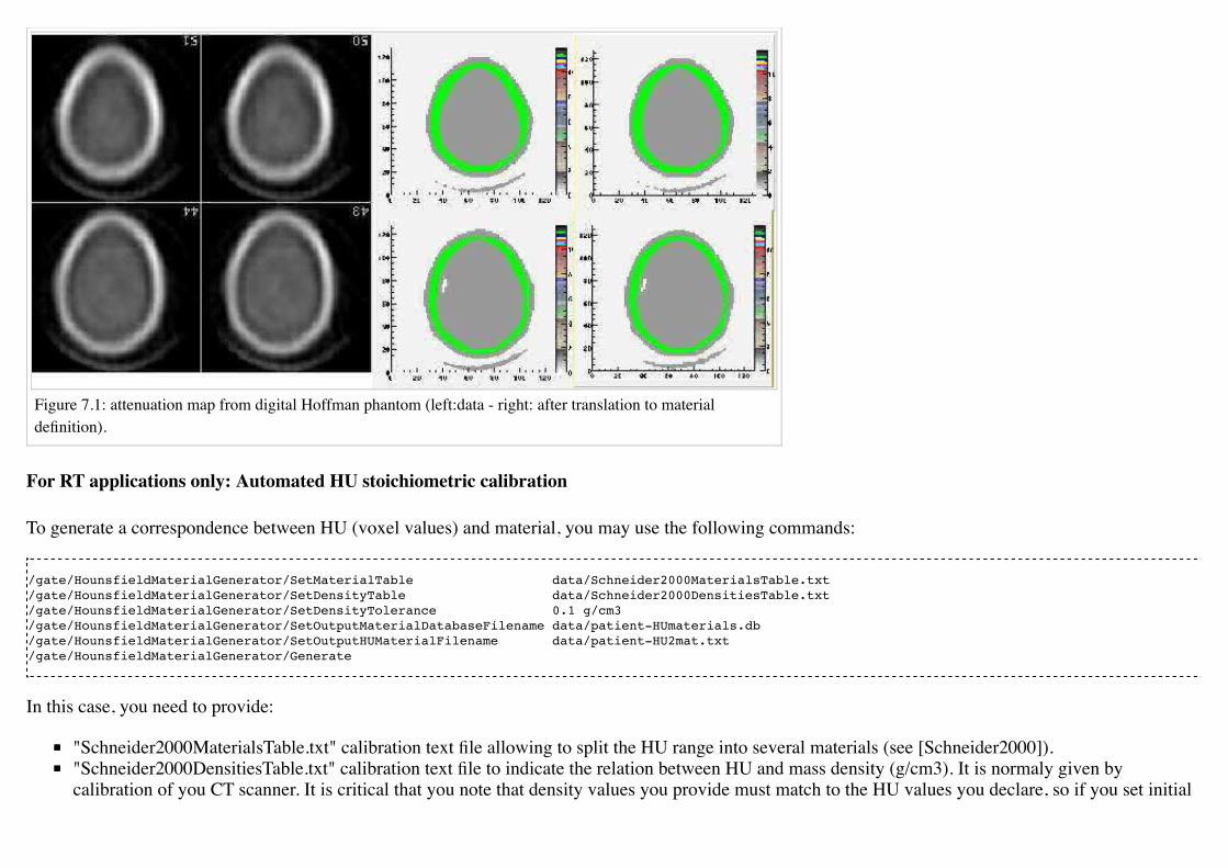
Figure 7.1: attenuation map from digital Hoffman phantom (left:data - right: after translation to materialdefinition).

For RT applications only: Automated HU stoichiometric calibration

To generate a correspondence between HU (voxel values) and material, you may use the following commands:

/gate/HounsfieldMaterialGenerator/SetMaterialTable data/Schneider2000MaterialsTable.txt /gate/HounsfieldMaterialGenerator/SetDensityTable data/Schneider2000DensitiesTable.txt/gate/HounsfieldMaterialGenerator/SetDensityTolerance 0.1 g/cm3/gate/HounsfieldMaterialGenerator/SetOutputMaterialDatabaseFilename data/patient-HUmaterials.db/gate/HounsfieldMaterialGenerator/SetOutputHUMaterialFilename data/patient-HU2mat.txt/gate/HounsfieldMaterialGenerator/Generate

In this case, you need to provide:

"Schneider2000MaterialsTable.txt" calibration text file allowing to split the HU range into several materials (see [Schneider2000])."Schneider2000DensitiesTable.txt" calibration text file to indicate the relation between HU and mass density (g/cm3). It is normaly given bycalibration of you CT scanner. It is critical that you note that density values you provide must match to the HU values you declare, so if you set initial

HU values for the materials you have to provide initial density values also. It is a common mistake that you provide the mean density, making Gateoverestimate it when perform the interpolation, so be careful.the parameter "DensityTolerance" allows the user to define the density tolerance. Even if it is possible to generate a new Geant4 material (atomiccomposition and density) for each different HU, it would lead to too much different materials, with a long initialization time. So we define a singlematerial for a range of HU belonging to the same material range (in the first calibration Table) and with densities differing for less than the tolerancevalue.the files "patient-HUmaterials.db" and "patient-HU2mat.txt" are generated and can be used with setMaterialDatabase and SetHUToMaterialFilemacros.

Examples are available here (http://wiki.opengatecollaboration.org/?title=GateRT)

Voxelized sourcesSince release V7.1, possibilities to read in voxellized sources within GATE have been extended. They all require the user to provide 3D image stored in oneof the following formats: Interfile (8-bit, 16- or 32-bit Signed and Unsigned, and 32- or 64-bit Real), Analyze, MetaImage and DICOM.

Conversion into activity values

Each voxel of the grayscale image is converted into actual activity value using either a linear or a range (same kind as the voxelized phantom one)translation table.

An example of a range translation table from voxel encoded values to activities (ActivityRange.dat in the example) is shown below:

34 4 15 5 314 15 5

where you specify the number of subdivisions or intervals (3 in this example), followed by the intervals definition and the correlated activity attached to eachinterval. If the number in the ASCII file, for a given voxel, is for instance between 14 and 15, then the activity for that voxel is set to 5. Bq. The resultingvoxelized source has thus a discretized number of activity values (preliminar segmentation).

Example of voxelized source description macro

Example of voxelized source description macro reading in an InterFile image as source distributions is detailed below:

!!!WARNING: Macro commands related to voxelized source description have been modified in GATE V7.1!!!Older ones are being deprecated and will be removed from the next release

# DECLARATION OF THE FACT THAT A VOXELIZED SOURCE WILL BE USED # Always use the keyword voxel to declare the type/gate/source/addSource hof_brain voxel# DECLARATION THAT THE VOXELIZED SOURCE WILL BE ENTERED USING IMAGE DATA/gate/source/hof_brain/reader/insert image # INSERT THE TRANSLATOR THAT WILL CONVERT THE IMAGE FROM DIGITAL VALUES TO ACTIVITY VALUES # Example for a linear translator: this scales all image values directly into activities/gate/source/hof_brain/imageReader/translator/insert linear/gate/source/hof_brain/imageReader/linearTranslator/setScale 1. Bq# Example for a range translator (can not be used simultaneously)# Here the values of the image file are discretized in intervals and are then converted to predefined activities /gate/source/hof_brain/imageReader/translator/insert range /gate/source/hof_brain/imageReader/rangeTranslator/readTable ActivityRange.dat /gate/source/hof_brain/imageReader/rangeTranslator/describe 1 # THE FOLLOWING LINE ALLOWS YOU TO INSERT THE IMAGE DATA USING THE APPROPRIATE EXTENSION FILE/gate/source/hof_brain/imageReader/readFile hof_brain_phantom.h33 /gate/source/hof_brain/imageReader/verbose 1

# THE DEFAULT POSITION OF THE VOXELIZED SOURCE IS IN THE 1ST QUARTER# SO THE VOXELIZED SOURCE HAS TO BE SHIFTED OVER HALF ITS DIMENSION IN THE NEGATIVE DIRECTION ON EACH AXIS /gate/source/hof_brain/setPosition -128. -128. 0. mm /gate/source/hof_brain/dump 1

# THE FOLLOWING LINES CHARACTERIZE THE SIZE (NO DIFFERENCE WITH AN ANALYTICAL SOURCE) /gate/source/voxel/setType backtoback /gate/source/voxel/gps/particle gamma /gate/source/voxel/gps/energytype Mono /gate/source/voxel/gps/monoenergy 140. keV /gate/source/voxel/gps/angtype iso /gate/source/voxel/gps/mintheta 0. deg /gate/source/voxel/gps/maxtheta 90. deg /gate/source/voxel/gps/minphi 0. deg /gate/source/voxel/gps/maxphi 360. deg /gate/source/voxel/gps/confine NULL

Using this image file reader any digital phantom or patient data, stored in any image format among ASCII, Interfile, Analyze, MetaImage and DICOM, canbe read in as emission distribution. Afterwards, activity levels can be used to determine the number of primary particles for each voxel.

An example of the Hoffman brain phantom, where the gray scales have been translated to activity distributions is shown in Figure 7.2.

Figure 7.2: emission map from digital Hoffman phantom (left:data - right: translatedactivity values).

Dose collectionTo collect absorbed dose deposited in the phantom, attach the phantom sensitive detector with the new attachVoxelPhantomSD command (and notattachPhantomSD) and add a dose output module:

/gate/anyname/attachVoxelPhantomSD /gate/anyname/addOutput outputModuleName

The output module responds to the following commands:

/gate/output/outputModuleName/saveUncertainty [true|false] /gate/output/outputModuleName/setFileName anyFileName

The output file is a binary file (number format is 4 bytes float) containing the absorbed dose in cGy. It has the same dimensions as the phantom. The outputmodule optionally writes a second binary file containing the uncertainty on absorbed dose expressed as a fraction between 0 and 1. The uncertainty file alsohas the same dimensions as the phantom and its creation is controlled by the saveUncertainty command. The file name is the same as the absorbed dose file

with a capital U appended. By default, the output file name is doseMatrix.bin and the uncertainty file is not created.

Example

# Create a simple phantom called CCD /gate/world/daughters/name CCD /gate/world/daughters/insert parameterizedBoxMatrix

# Read the file : a 300x300x1 array /gate/CCD/geometry/insertReader image /gate/CCD/imageReader/insertTranslator tabulated /gate/CCD/imageReader/tabulatedTranslator/readTable ccdTable.dat /gate/CCD/imageReader/readFile ccd300Phantom.dat

# Place the phantom and rotate it so that it is in the XZ plane /gate/CCD/placement/setTranslation 0 -82.269 0 mm /gate/CCD/placement/setRotationAxis 1 0 0 /gate/CCD/placement/setRotationAngle 90 deg

# Attach the phantom SD and the output module /gate/CCD/attachVoxelPhantomSD /gate/CCD/addOutput doseOutput /gate/output/doseOutput/saveUncertainty true /gate/output/doseOutput/setFileName ccdDose.bin

Comments

Depending on the phantom dimensions, the use of a parameterizedBoxMatrix may increase memory usage by up to a factor of 2 and increase CPU time by5-50.

If you plan to collect only dose in the phantom, it is suggested that you disable other types of output, for example:

/gate/output/ascii/disable

Dose calculations

The relative uncertainty on dose is calculated on a per voxel basis. Let be the sequence of energy deposits in a given voxel, we cancalculate the following quantities:

Mean energy deposit:

Figure 7.2: A simple voxellized phantomwithout transparency

Sample variance:

Population variance estimator:

Standard deviation:

Standard error of the mean:

Real-time motion management for voxellized source and phantomGenerate N frames for the phantom corresponding to the time acquisition desired for example 50 frames for 5s so each frame is for .1 s ;I assume the 50 frames are NCAT_frame_.i33, NCAT_frame_2.i33, NCAT_frame_3.i33, NCAT_frame_4.i33 $...$ NCAT_frame_N.i33.

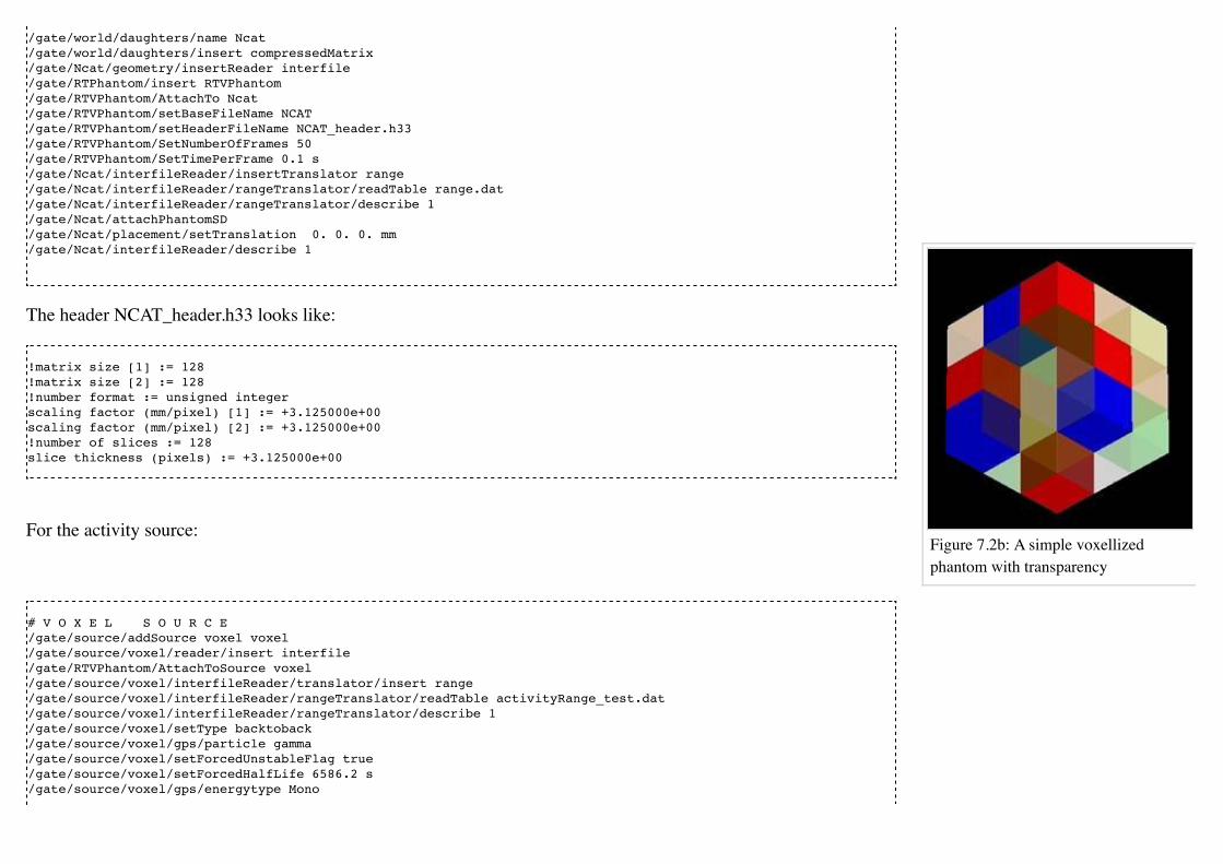
Figure 7.2b: A simple voxellizedphantom with transparency

/gate/world/daughters/name Ncat/gate/world/daughters/insert compressedMatrix/gate/Ncat/geometry/insertReader interfile/gate/RTPhantom/insert RTVPhantom/gate/RTVPhantom/AttachTo Ncat/gate/RTVPhantom/setBaseFileName NCAT/gate/RTVPhantom/setHeaderFileName NCAT_header.h33/gate/RTVPhantom/SetNumberOfFrames 50/gate/RTVPhantom/SetTimePerFrame 0.1 s/gate/Ncat/interfileReader/insertTranslator range/gate/Ncat/interfileReader/rangeTranslator/readTable range.dat/gate/Ncat/interfileReader/rangeTranslator/describe 1/gate/Ncat/attachPhantomSD/gate/Ncat/placement/setTranslation 0. 0. 0. mm/gate/Ncat/interfileReader/describe 1

The header NCAT_header.h33 looks like:

!matrix size [1] := 128 !matrix size [2] := 128 !number format := unsigned integer scaling factor (mm/pixel) [1] := +3.125000e+00 scaling factor (mm/pixel) [2] := +3.125000e+00 !number of slices := 128 slice thickness (pixels) := +3.125000e+00

For the activity source:

# V O X E L S O U R C E/gate/source/addSource voxel voxel/gate/source/voxel/reader/insert interfile/gate/RTVPhantom/AttachToSource voxel/gate/source/voxel/interfileReader/translator/insert range/gate/source/voxel/interfileReader/rangeTranslator/readTable activityRange_test.dat/gate/source/voxel/interfileReader/rangeTranslator/describe 1/gate/source/voxel/setType backtoback/gate/source/voxel/gps/particle gamma/gate/source/voxel/setForcedUnstableFlag true/gate/source/voxel/setForcedHalfLife 6586.2 s/gate/source/voxel/gps/energytype Mono

/gate/source/voxel/gps/monoenergy 0.511 MeV/gate/source/voxel/setPosition -200. -200. -200 mm/gate/source/voxel/gps/confine NULL/gate/source/voxel/gps/angtype iso/gate/source/voxel/dump 1

#TIME ACTIVITY option/gate/source/voxel/interfileReader/SetTimeActivityTablesFrom TimeActivity_Tables.dat/gate/source/voxel/interfileReader/SetTimeSampling 0.001 s

The activityRange_test.dat is a text file looking like this:

1246 46 061 61 0123 123 0215 215 0246 246 0261 261 0352 352 352369 369 0770 770 0831 831 02300 2300 0950 950 950

The TimeActivity_Tables.dat is a text file looking like this:

2950 lesion.dat352 liver.dat

Where the value 950 is the key corresponding in the attenuation map to the lesion and 352 is the key corresponding in the attenuation map to the liver.\\ Notethat lesion.dat is a text file which contains the time activity table curve for the lesion, as explain here:

19

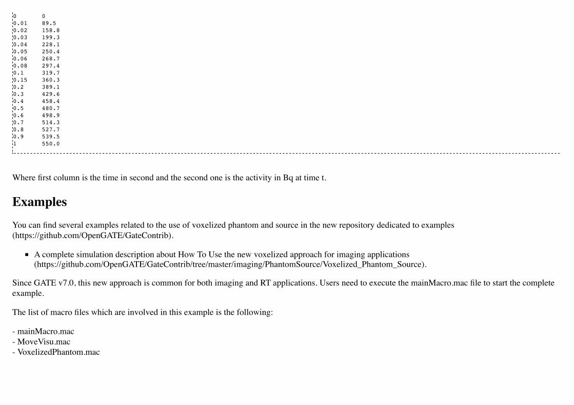
0 00.01 89.50.02 158.80.03 199.30.04 228.10.05 250.40.06 268.70.08 297.40.1 319.70.15 360.30.2 389.10.3 429.60.4 458.40.5 480.70.6 498.90.7 514.30.8 527.70.9 539.51 550.0

Where first column is the time in second and the second one is the activity in Bq at time t.

ExamplesYou can find several examples related to the use of voxelized phantom and source in the new repository dedicated to examples(https://github.com/OpenGATE/GateContrib).

A complete simulation description about How To Use the new voxelized approach for imaging applications(https://github.com/OpenGATE/GateContrib/tree/master/imaging/PhantomSource/Voxelized_Phantom_Source).

Since GATE v7.0, this new approach is common for both imaging and RT applications. Users need to execute the mainMacro.mac file to start the completeexample.

The list of macro files which are involved in this example is the following:

- mainMacro.mac- MoveVisu.mac- VoxelizedPhantom.mac

- VoxelizedSource.mac- MoveVisu.mac- Verbose.mac

The phantom used in this application (Interfile Format)

- Raw data: brain_phantom.i33- Header file: brain_phantom.h33

And the associated ASCII files to convert phantom voxel values in material properties and activity values

- range_atten_brain.dat- activity_range_brain.dat

Example of photon beam in patient CT image (https://github.com/OpenGATE/GateContrib/tree/master/dosimetry/Radiotherapy/example2)

Two different navigators are tested NestedParameterized and Regionalized, with two number of materials.

Output is a 3D dose distribution map (with associated uncertainty).

Comparison between MetaImage and DICOM formats (https://github.com/OpenGATE/GateContrib/tree/master/imaging/DICOM/mhd-dcm-comparison)

The main simulation files are constructed as follows:

- main-[series name]-[input format].mac- [series name] : ffp, ffs, hfp, hfs- [input format]: mhd, dcm

Each main file will generate two mhd images:

- one containing the density dump of the image (density-[series name]-[input format].mhd/.raw)- one containing the deposited dose in the image (DA-[series name]-[input format]-Dose.mhd/.raw)

Comparison between input formats can be made by the diff command:

diff DA-[seriesA]-mhd-Dose.raw DA-[seriesA]-dcm-Dose.raw

Retrieved from "http://wiki.opengatecollaboration.org/index.php?title=Users_Guide_V8.0:Voxelized_Source_and_Phantom&oldid=1030"


Users Guide V8.0:Tools to Interact with the Simulation : ActorsFrom Wiki OpenGATE

Contents1 General Purpose

1.1 Add an actor1.2 Attach to a volume1.3 Save output1.4 3D matrix actor (Image actor)

2 List of available Actors2.1 Simulation statistic2.2 Electromagnetic (EM) properties2.3 Dose measurement

2.3.1 Dose calculation algorithms2.3.1.1 Volume weighting algorithm2.3.1.2 Mass weighting algorithm

2.4 Kill track2.5 Stop on script2.6 Track length2.7 Energy spectrum2.8 Production and stopping particle position2.9 Secondary production2.10 Delta kinetic energy2.11 Number of particles entering volume2.12 Q-value2.13 CrossSectionProductionActor2.14 WashOutActor2.15 Fluence Actor (particle counting)2.16 TLE and seTLE (Track Length Estimator)2.17 Fixed Forced Detection CT2.18 Fixed Forced Detection SPECT

2.19 PromptGammaTLEActor2.20 LET Actor2.21 Tissue Equivalent Proportional Counter Actor2.22 Phase Space Actor2.23 Thermal Actor2.24 Merged Volume Actor

3 Filters3.1 Filter on particle type3.2 Filter on particle ID3.3 Filter on volume3.4 Filter on energy3.5 Filter on direction

Actors are tools which allow to interact with the simulation. They can collect information during the simulation, such as energy deposit, number of particlescreated in a given volume, etc. They can also modify the behavior of the simulation. Actors use hooks in the simulation : run (begin/end), event(begin/end),track(begin/end), step.

General Purpose

Add an actor

/gate/actor/addActor [Actor Type] [Actor Name]

Attach to a volume

Tells that the actor is attached to the volume [Volume Name]. For track and step levels, the actor is activated for step inside the volume and for tracks createdin the volume. If no attach command is provided then the actor is activated in any volume. The children of the volume inherit the actor.

/gate/actor/[Actor Name]/attachTo [Volume Name]

Save output

This command allow to save the data of the actor to the file [File Name]. The particular behaviour (format, etc.) depends on the type of the actor.

/gate/actor/[Actor Name]/save [File Name]

It is possible to save the output every N events with the command:

/gate/actor/[Actor Name]/saveEveryNEvents [N]

It is possible to save the output every N seconds with the command:

/gate/actor/[Actor Name]/saveEveryNSeconds [N]

3D matrix actor (Image actor)

Some actors, such as the dose actor, can store some information into a 3D image (or matrix) according to the spatial position of the hit. User can specify theresolution of the 3D matrix. Alternatively, user can specify the size to allow larger of smaller matrices.

"attachTo" : the scoring value is stored in the 3D matrix only when a hit occur in the attached volume. If the size of the volume is greater than the 3Dmatrix, hit occurring out of the matrix are not recorded. Conversely, if the 3D matrix is larger than the attached volume, part which is outside thevolume will never record hit (even if it occurs) because hit is performed out of the volume."type" : In Geant4, when a hit occurs, the energy is deposited along a step line. A step is defined by two positions the 'PreStep' and the 'PostStep'. Theuser can choose at which position the actor have to store the information (edep, dose ...) : it can be at PreStep ('pre'), at PostStep ('post'), at the middlebetween PreStep and PostStep ('middle') or distributed from PreStep to PostStep ('random'). According to the matrix size, such line can be locatedinside a single dosel or cross several dosels. Preferred type of hit is "random", meaning that a random position is computed along this step line and allthe energy is deposited inside the dosel that contains this point.the attached volume can be a voxelized image. The scoring matrix volume (dosels) are thus different from the geometric voxels describing the image.

/gate/actor/[Actor Name]/attachTo waterbox/gate/actor/[Actor Name]/setSize 5 5 5 cm/gate/actor/[Actor Name]/voxelsize 10 20 5 mm/gate/actor/[Actor Name]/setPosition 1 0 0 mm/gate/actor/[Actor Name]/stepHitType random

If you would like the dose actor to use exactly the same voxels as the input image, then the safest way to configure this is with setResolution.

Otherwise, when setting voxelsize, rounding errors may cause the dosels to be slightly different, in particular in cases where the voxel size is not anice round number (e.g. 1.03516 mm on a dimension with 512 voxels). Such undesired rounding effects have been observed Gate release 7.2 and maybe fixed in a later release.

List of available Actors

Simulation statistic

This actor counts the number of steps, tracks, events, runs in the simulation. If the actor is attached to a volume, the actor counts the number of steps andtracks in the volume. The output is an ASCII file.

/gate/actor/addActor SimulationStatisticActor MyActor/gate/actor/MyActor/save MyOutput.txt

Electromagnetic (EM) properties

This actor allows extracting EM properties for all materials defined in a simulation, as listed below :

Density (mass density in g/cm³)e-density (electronic density in e-/mm³)RadLength (radiation length in mm)I (ionization potential in eV)EM-DEDX (EM mass stopping power in MeV.cm²/g)Nucl-DEDX (nuclear mass stopping power in MeV.cm²/g)Tot-DEDX (total mass stopping power in MeV.cm²/g)

EM properties are calculated relative to a specific particle type and energy, as defined by the user. For instance, EM properties corresponding to a 30 MeVneutron can be calculated using the following command lines:

/gate/actor/addActor EmCalculatorActor MyActor/gate/actor/MyActor/setParticleName proton/gate/actor/MyActor/setEnergy 150 MeV/gate/actor/MyActor/save MyOutput.txt

Dose measurement

The DoseActor builds 3D images of the energy deposited (edep), dose deposited and the number of hits in a given volume. It takes into account the weightof particles. It can store multiple information into a 3D grid, each information can be enabled by using:

/gate/actor/[Actor Name]/enableEdep true/gate/actor/[Actor Name]/enableUncertaintyEdep true/gate/actor/[Actor Name]/enableSquaredEdep true/gate/actor/[Actor Name]/enableDose true/gate/actor/[Actor Name]/enableUncertaintyDose true/gate/actor/[Actor Name]/enableDose true/gate/actor/[Actor Name]/enableUncertaintyDose true/gate/actor/[Actor Name]/enableSquaredDose true/gate/actor/[Actor Name]/enableNumberOfHits true

Informations can be disable by using "false" instead of "true" (by default all states are false):

/gate/actor/[Actor Name]/enableEdep false

The unit of edep is MeV and the unit of dose is Gy. The dose/edep squared is used to calculate the uncertainty when the output from several files are added.The uncertainty is the relative statistical uncertainty. "SquaredDose" flag allows to store the sum of squared dose (or energy). It is very useful when usingGATE on several workstations with numerous jobs. To compute the final uncertainty, you only have to sum the dose map and the squared dose map toestimate the final uncertainty according to the uncertainty equations.

It is possible to normalize the maximum dose value to 1:

/gate/actor/[Actor Name]/normaliseDose true

For the output, the suffixes Edep, Dose, NbOfHits, Edep-Uncertainty, Dose-Uncertainty, Edep-Squared or Dose-Squared are added to the output file namegiven by the user. You can use several files types: ASCII file (.txt), root file (.root), Analyze (.hdr/.img) and MetaImage (.mhd/.raw) (mhd isrecommended !). The root file works only for 1D and 2D distributions.

/gate/actor/addActor DoseActor MyActor/gate/actor/MyActor/save MyOutputFile.mhd/gate/actor/MyActor/attachTo MyVolume/gate/actor/MyActor/stepHitType random

/gate/actor/MyActor/setSize 5 5 5 m/gate/actor/MyActor/setResolution 1 1 3000 /gate/actor/MyActor/enableEdep true/gate/actor/MyActor/enableUncertaintyEdep true/gate/actor/MyActor/enableSquaredEdep false/gate/actor/MyActor/enableDose false/gate/actor/MyActor/normaliseDose false

Water equivalent doses (or dose to water) can be also calculated, in order to estimate doses calculated using water equivalent path length approximations,such as in Treatment Planning Systems (TPS). Command previously presented for the "dose" also work for the "dose to water" as shown below:

/gate/actor/[Actor Name]/enableDoseToWater true/gate/actor/[Actor Name]/enableUncertaintyDoseToWater true/gate/actor/[Actor Name]/normaliseDoseToWater true

New image format : MHD

Gate now can read and write mhd/raw image file format. This format is similar to the previous hdr/img one but should solve a number of issues. To use it,just specify .mhd as extension instead of .hdr. The principal difference is that mhd store the 'origin' of the image, which is the coordinate of the (0,0,0) pixelexpressed in the physical world coordinate system (in general in millimetres). Typically, if you get a DICOM image and convert it into mhd (vv(http://vv.creatis.insa-lyon.fr) can conveniently do this), the mhd will keep the same pixels coordinate system than the DICOM.

In GATE, if you specify the macro "TranslateTheImageAtThisIsoCenter" with the coordinate of the isocenter that is in a DICOM-RT-plan file, the imagewill be placed such that this isocenter is at position (0,0,0) of the mother volume (often the world). This is very useful to precisely position the image asindicated in a RT plan. Also, when using a DoseActor attached to a mhd file, the output dose distribution can be stored in mhd format. In this case, the originof the dose distribution will be set such that it corresponds to the attached image (easy superimposition display).

Note however, that the mhd module is still experimental and not complete. It is thus possible that some mhd images cannot be read. Use and enjoy at yourown risk, please contact us if you find bugs and be warmly acknowledged if you correct bugs.

Dose calculation algorithms

When storing a dose (D=edep/mass) with the DoseActor, mass is computed by using the material density at the step location and using the volume the dosel.If the size of the image voxel is smaller than the size of the dosel of the DoseActor it can lead to undesired results. Two algorithms are available for theDoseActor.

Volume weighting algorithm

This algorithm is used by default. The absorbed dose of each material is ponderated by the fraction of materials volume.

/gate/actor/[Actor Name]/setDoseAlgorithm VolumeWeighting

Mass weighting algorithm

This algorithm calculates the dose of each dosels by taking the deposited energy and dividing it by its mass.

/gate/actor/[Actor Name]/setDoseAlgorithm MassWeighting

Mass image :

Mass images (.txt, .root, .mhd) can be imported and exported to be used by the mass weighting algorithm.

Exportation :

/gate/actor/[Actor Name]/exportMassImage path/to/MassImage

Importation :

/gate/actor/[Actor Name]/importMassImage path/to/MassImage

The unit of mass images is kg.

When the mass weighting algorithm is used on a unvoxelized volume, depending on the dosel's resolution of the DoseActor the computation can takea very long time.

Important note : If no mass image is imported when using the mass weighting algorithm Gate will calculate the mass during the simulation (this cantake a lot of time).

The command 'exportMassImage' can be used to generate the mass image of the DoseActor attached volume one time for all and import it with the'importMassFile' command.

Limitations :

With voxelized phantom :MassWeighting algorithm work with phantoms imported with ImageRegularParametrisedVolume and ImageNestedParametrisedVolume.For now it's not possible to choose an actor resolution smaller than the phantom's resolution.It is mandatory to attach directly the phantom to the actor.

With unvoxelized geometry : The dosels resolution must be reasonably low otherwise the time of calculation can be excessively long ! (and can needa lot of memory !)

Kill track

This actor kills tracks entering the volume. The output is the number of tracks killed. It is stored an ASCII file.

/gate/actor/addActor KillActor MyActor/gate/actor/MyActor/save MyOutputFile.txt/gate/actor/MyActor/attachTo MyVolume

Stop on script

This actor gets the output of a script and stop the simulation if this output is true.

/gate/actor/addActor StopOnScriptActor MyActor/gate/actor/MyActor/save MyScript

It is possible to save all the other actors before stopping the simulation with the command :

/gate/actor/MyActor/saveAllActors true

Track length

This actor stores the length of each tracks in a root file. It takes into account the weight of particles. They are three commands to define the boundaries andthe binning of the histogram.

/gate/actor/addActor TrackLengthActor MyActor/gate/actor/MyActor/save MyOutputFile.root/gate/actor/MyActor/setLmin 0 mm/gate/actor/MyActor/setLmax 1 cm/gate/actor/MyActor/setNumberOfBins 200

Energy spectrum

This actor builds four histograms : the initial kinetic energy of each track ('energySpectrum'), the energy deposition per event ('edepHisto'), the energydeposition per track ('edepTrackHisto') and the energy loss per track ('eLossHisto'). These histograms are stored in a root file. They take into account theweight of particles.

/gate/actor/addActor EnergySpectrumActor MyActor/gate/actor/MyActor/save MyOutputFile.root/gate/actor/MyActor/energySpectrum/setEmin 0 eV/gate/actor/MyActor/energySpectrum/setEmax 10 GeV/gate/actor/MyActor/energySpectrum/setNumberOfBins 200/gate/actor/MyActor/energyLossHisto/setEmin 0 eV/gate/actor/MyActor/energyLossHisto/setEmax 15 MeV/gate/actor/MyActor/energyLossHisto/setNumberOfBins 120

Production and stopping particle position

This actor stores in a 3D image the position where particles are produced and where particles are stopped. For the output, the suffixes 'Prod' and 'Stop' areadded to the output file name given by the user. You can use several files types: ASCII file (.txt), root file (.root), (.hdr/.img). The root file works only for 1Dand 2D distribution.

/gate/actor/addActor ProductionAndStoppingActor MyActor/gate/actor/MyActor/save MyOutputFile.hdr/gate/actor/MyActor/attachTo MyVolume/gate/actor/MyActor/setResolution 10 10 100/gate/actor/MyActor/stepHitType post

< ! > In Geant4, secondary production occurs at the end of the step, the recommended state for 'stepHitType' is 'post'

Secondary production

This actor creates a root file and stores the number of secondaries in function of the particle type. Ionisation electrons are dissociated from electronsproduced by other processes. Decay positrons are dissociated from positrons produced by other processes. Gammas are classified in four categories: gammasproduced by EM processes, gammas produced by hadronic processes, gammas produced by decay processes and other gammas.

/gate/actor/addActor SecondaryProductionActor MyActor/gate/actor/MyActor/save MyOutputFile.root/gate/actor/MyActor/attachTo MyVolume

Delta kinetic energy

This actor sums the relative and absolute (kinetic energy) and stores the results in two files (with suffixes "-RelStopPower" and "-StopPower"). It alsostores the map of the hits to allow users to calculate the mean values.

/gate/actor/addActor StoppingPowerActor MyActor/gate/actor/MyActor/save MyOutputFile.hdr/gate/actor/MyActor/attachTo MyVolume/gate/actor/MyActor/setResolution 10 10 100/gate/actor/MyActor/stepHitType random

Number of particles entering volume

This actor builds a map of the number of particules produced outside of the actor volume and interacting in the volume. The particle is recorded once in eachvoxel where it interacting.

/gate/actor/addActor ParticleInVolumeActor MyActor/gate/actor/MyActor/save MyOutputFile.hdr/gate/actor/MyActor/attachTo MyVolume/gate/actor/MyActor/setResolution 10 10 100/gate/actor/MyActor/stepHitType post

Q-value

This actor calculates the Q-values of interactions.

/gate/actor/addActor QvalueActor MyActor/gate/actor/MyActor/save MyOutputFile.hdr/gate/actor/MyActor/attachTo MyVolume/gate/actor/MyActor/setResolution 10 10 100/gate/actor/MyActor/stepHitType random

CrossSectionProductionActor

The CrossSectionProductionActor derives the production of C-11 or O-15 from the equation proposed by (Parodi et al, 2007). The cross section data areprovided directly in the class code. By default, only the production of the C-11 is activated.

WARNING: The size of the image has to be given in mm

The current limit in cross section data is 199 MeV. Other data can be added in the class.

/gate/actor/addActor CrossSectionProductionActor beta/gate/actor/beta/attachTo volume/gate/actor/beta/save output_dump/test_small.hdr/gate/actor/beta/addO15 true/gate/actor/beta/addC11 true/gate/actor/beta/setVoxelSize 1 1 1 mm/gate/actor/beta/saveEveryNEvents 100000

WashOutActor

The bilogical washout follows the Mizuno model (H. Mizuno et al. Phys. Med. Biol. 48, 2003). The activity distributions of the washout actor associatedvolume are continuously modified as a function of the acquisition time in terms of the following equation :

Where 3 components are defined (fast, medium and slow) with two parameters for each : the half life T and the fraction M (Mf + Mm + Ms = 1).

Users should provide a table as an ASCII file with the washout parameters values for any radioactive source in the associated volume. In order to take intoaccount the physiological properties of each tissue, it is important to highlight that one independent radioactive source should be defined per each materialinvolved in the simulation.

/gate/actor/addActor WashOutActor [ACTOR NAME]/gate/actor/[ACTOR NAME]/attachTo [VOLUME NAME]/gate/actor/[ACTOR NAME]/readTable [TABLE FILE NAME]

Example of [TABLE FILE NAME]: How to specify different parameters which are associated to the washout model - This ASCII file will be used by thewashout Actor.

2 [SOURCE 1 NAME] [MATERIAL 1 NAME] [Mf VALUE] [Tf VALUE IN SEC] [Mm VALUE] [Tm VALUE IN SEC] [Ms VALUE] [Ts VALUE IN SEC] [SOURCE 2 NAME] [MATERIAL 2 NAME] [Mf VALUE] [Tf VALUE IN SEC] [Mm VALUE] [Tm VALUE IN SEC] [Ms VALUE] [Ts VALUE IN SEC] ......

Fluence Actor (particle counting)

This actor counts the number of time a (new) particle is passing through a volume ; output as an image.

/gate/actor/addActor FluenceActor Detector/gate/actor/Detector/save output/detector.mhd/gate/actor/Detector/attachTo DetectorPlane/gate/actor/Detector/stepHitType pre/gate/actor/Detector/setSize 10 410 410 mm/gate/actor/Detector/setResolution 1 256 256/gate/actor/Detector/enableScatter true

TLE and seTLE (Track Length Estimator)

TLE is the Track Length Estimator method initially proposed by [Williamson1997] allowing very fast dose computation for low energy photon beam (aboutbelow 1 MeV). About 1000x faster than analog Monte-Carlo. The second method, seTLE for split-exponential TLE, was proposed in [Smekens2014] and isabout 15x faster than TLE.

Williamson J F 1987 Monte Carlo evaluation of kerma at a point for photon transport problems Med. Phys. 14 567–76F. Smekens, J. M. Létang, C. Noblet, S. Chiavassa, G. Delpon, N. Freud, S. Rit, and D. Sarrut, "Split exponential track length estimator for Monte-Carlo simulations of small-animal radiation therapy", Physics in medicine and biology, vol. 59, issue 24, pp. 7703-7715, 2014 [[1](http://iopscience.iop.org/0031-9155/59/24/7703/pdf/0031-9155_59_24_7703.pdf%7Cpdf)]F. Baldacci, A. Mittone, A. Bravin, P. Coan, F. Delaire, C. Ferrero, S. Gasilov, J. M. Létang, D. Sarrut, F. Smekens, et al., "A track length estimatormethod for dose calculations in low-energy x-ray irradiations: implementation, properties and performance", Zeitschrift Fur Medizinische Physik,2014.A. Mittone, F. Baldacci, A. Bravin, E. Brun, F. Delaire, C. Ferrero, S. Gasilov, N. Freud, J. M. Létang, D. Sarrut, et al., "An efficient numerical tool fordose deposition prediction applied to synchrotron medical imaging and radiation therapy.", Journal of synchrotron radiation, vol. 20, issue Pt 5, pp.785-92, 2013

Usage is very simple just replace the DoseActor by TLEDoseActor. See examples/example_Radiotherapy/example10 in the Gate source code :

/gate/actor/addActor TLEDoseActor tle/gate/actor/tle/attachTo phantom/gate/actor/tle/stepHitType random/gate/actor/tle/setVoxelSize 2 2 2 mm/gate/actor/tle/enableDose true/gate/actor/tle/save output/dose-tle.mhd

or

/gate/actor/addActor SETLEDoseActor setle/gate/actor/setle/attachTo phantom/gate/actor/setle/setVoxelSize 2 2 2 mm/gate/actor/setle/enableHybridino true/gate/actor/setle/setPrimaryMultiplicity 200/gate/actor/setle/setSecondaryMultiplicity 400/gate/actor/setle/enableDose true/gate/actor/setle/save output/dose-setle.mhd

A detailed documentation is available here : http://midas3.kitware.com/midas/download/item/316877/seTLE.pdf

Fixed Forced Detection CT

This actor is a Variance Reduction Technique for the simulation of CT.

The fixed forced detection technique (Colijn & Beekman 2004, Freud et al. 2005, Poludniowski et al. 2009) relies on the deterministic computation of theprobability of the scattered photons to be aimed at each pixel of the detector. The image of scattered photons is obtained from the sum of these probabilities.

The probability of each scattering point to contribute to the center of the j−th pixel is the product of two terms:

the probability of the photon to be scattered in the direction of the pixel

the probability of the scattered photon to reach the detector and to be detected

Fixed Forced Detection summary

1) Deterministic simulation of the primary (DRR)

2) Low statistics Monte Carlo simulation ⇒ Compute scattering points

3) Fixed forced detection (deterministic)

Inputs:

/gate/actor/addActor FixedForcedDetectionActor MyActor/gate/actor/MyActor/attachTo world/gate/actor/MyActor/setDetector DetectorPlane/gate/actor/MyActor/setDetectorResolution 128 128/gate/actor/MyActor/responseDetectorFilename responseDetector.txt

The detector response δ(E) is modeled with a continuous energy-function that describes the average measured energy for a given incident energy E.

attachTo ⇒ Attaches the sensor to the given volumesaveEveryNEvents ⇒ Save sensor every n Events.saveEveryNSeconds ⇒ Save sensor every n seconds.addFilter ⇒ Add a new filtersetDetector ⇒ Set the name of the volume used for detector (must be a Box).setDetectorResolution ⇒ Set the resolution of the detector (2D).

geometryFilename ⇒ Set the file name for the output RTK geometry filename corresponding to primary projections.primaryFilename ⇒ Set the file name for the primary x-rays (printf format with runId as a single parameter).materialMuFilename ⇒ Set the file name for the attenuation lookup table. Two paramaters: material index and energy.attenuationFilename ⇒ Set the file name for the attenuation image (printf format with runId as a single parameter).responseDetectorFilename ⇒ Input response detector curve.flatFieldFilename ⇒ Set the file name for the flat field image (printf format with runId as a single parameter).comptonFilename ⇒ Set the file name for the Compton image (printf format with runId as a single parameter).rayleighFilename ⇒ Set the file name for the Rayleigh image (printf format with runId as a single parameter).fluorescenceFilename ⇒ Set the file name for the fluorescence image (printf format with runId as a single parameter).secondaryFilename ⇒ Set the file name for the scatter image (printf format with runId as a single parameter).enableSquaredSecondary ⇒ Enable squared secondary computationenableUncertaintySecondary ⇒ Enable uncertainty secondary computationtotalFilename ⇒ Set the file name for the total (primary + scatter) image (printf format with runId as a single parameter).phaseSpaceFilename ⇒ Set the file name for storing all interactions in a phase space file in root format.setInputRTKGeometryFilename ⇒ Set filename for using an RTK geometry file as input geometry.noisePrimaryNumber ⇒ Set a number of primary for noise estimate in a phase space file in root format.

An example is available at example_CT/fixedForcedDetectionCT

The GateHybridForcedDetectionActor works for :

One voxelized (CT) volume, the rest must be of the same material as the world → No volume between voxelized volume and detector.

Point sources (plane distribution focused).

A given detector description.

With some additional geometric limitations.

Fixed Forced Detection SPECT

This actor is a Variance Reduction Technique for the simulation of SPECT.

The fixed forced detection technique (Colijn & Beekman 2004, Freud et al. 2005, Poludniowski et al. 2009) relies on the deterministic computation of theprobability of the scattered photons to be aimed at each pixel of the detector. The image of scattered photons is obtained from the sum of these probabilities.

The probability of each scattering point to contribute to the center of the j−th pixel is the product of two terms:

the probability of the photon to be scattered in the direction of the pixel

the probability of the scattered photon to reach the detector and to be detected

Inputs:

/gate/actor/addActor FixedForcedDetectionActor MyActor/gate/actor/MyActor/attachTo world/gate/actor/MyActor/setDetector DetectorPlane/gate/actor/MyActor/setDetectorResolution 128 128/gate/actor/MyActor/setSourceType isotropic/gate/actor/MyActor/generatePhotons trueor/gate/actor/MyActor/connectARF true

attachTo ⇒ Attaches the sensor to the given volumesetDetector ⇒ Set the name of the volume used for detector (must be a Box).setDetectorResolution ⇒ Set the resolution of the detector (2D).generatePhotons ⇒ Generates weighted photons outside of the volume directed at each pixel of the detector.connectARF ⇒ Connects the output of the FFD to ARF tables (see Users GuideV8.0:Digitizer_and_readout_parameters#Angular_Response_Functions_to_speed-up_planar_or_SPECT_simulations).

An example is available at GateContrib: SPECT_FFD (https://github.com/OpenGATE/GateContrib/tree/master/imaging/SPECT_FFD)

The GateHybridForcedDetectionActor works for :

One voxelized (CT) volume, the rest must be of the same material as the world → No volume between voxelized volume and detector.

With some additional geometric limitations.

PromptGammaTLEActor

This actor is used to investigate prompt gamma production in proton therapy simulations. It provides a speedup factor of around 1000 compared to analogMC. vpgTLE is broken up into three parts. Stage 0 is required to be run once, and each vpgTLE simulation is then broken up into Stage 1 and Stage 2. Foreach stage, you can find and example in the examples/vpgTLE directory.

To understand the background, physics and mathematics of this example, refer to Accelerated Prompt Gamma estimation for clinical Proton Therapysimulations by B.F.B. Huisman.

LET Actor

This actor calculates the dose or track averaged linear energy transfer.

/gate/actor/addActor LETActor MyActor/gate/actor/MyActor/save myLETactor.mhd/gate/actor/MyActor/attachTo phantom/gate/actor/MyActor/setResolution 1 1 100/gate/actor/MyActor/setType DoseAveraged

Options: DoseAveraged (default) or TrackAveraged. Both calculation methods use the Geant4 EMCalculator method "GetElectronicStoppingPowerDEDX".

For splitting the simulation into sevaral sub-simulations (e.g. parallel computation) enable:

/gate/actor/MyActor/doParallelCalculation true

The default value is false. Enabling this option will produce 2 output images for each LET actor and run, a file labeled as '-numerator' and one labeled as '-denominator'. Building the quotient of these two images results in the averaged LET image. Note that the numerator and denominator images have to besummed up before the division.

By default the unrestricted LET is calculated.

/gate/actor/MyActor/setRestricted false

If the restricted flag is set to true, the restricted LET is calculated, but also the calculation method changes. Instead of using tabulated stopping powers for themean kinetic energy of the particle, the stopping power is calculated as the quotient of the deposited energy and the step length (ICRU 85). Be aware ofpotential artifacts (voxel size, step limiter, e- production cuts etc.) reported in literature for this calculation method. The production cut for electrons definesthe energy carried away.

By default, the stopping power of the material at the PreStepPoint is used. If the averaged LET to water regardless of the material is of interest, set followingline to true:

/gate/actor/MyActor/setDoseToWater false

ID and particle filters can be used:

/gate/actor/MyActor/addFilter particleFilter/gate/actor/MyActor/particleFilter/addParticle proton

See: 'Cortes-Giraldo and Carabe, 2014, A critical study on different Monte Carlo scoring method of dose-average-linear energy transfer maps.'

Tissue Equivalent Proportional Counter Actor

The tissue-equivalent proportional counter (TEPC) is a detector dedicated to the measurement of the lineal energy transfer (LET) distribution in a volume atthe micrometric scale.These physical data, depending on the beam quality and the location of the detector in the beam, is mainly used to calculate thebiological dose for high LET radiation and to characterize the beam quality for radioprotection issues.

A TEPC is very similar to a classical gas ionization chamber. The major difference relies in the sensible volume, which is spherical and filled with lowpressure tissue -equivalent gas instead of air. These characteristics allow the TEPC to mimic the shape and composition of the tiny structures in a cellnucleus (about 1 μm of diameter).

Quick use

The principle of the TEPCactor is the same as the EnergySpectrumActor, except that the frequency of lineal energy is stored instead of the deposited energy.

In order to obtain the lineal energy, the deposited energy is divided by the mean chord of the TEPC volume ( ). This imposes creating a

sphere as geometry for the TEPC.

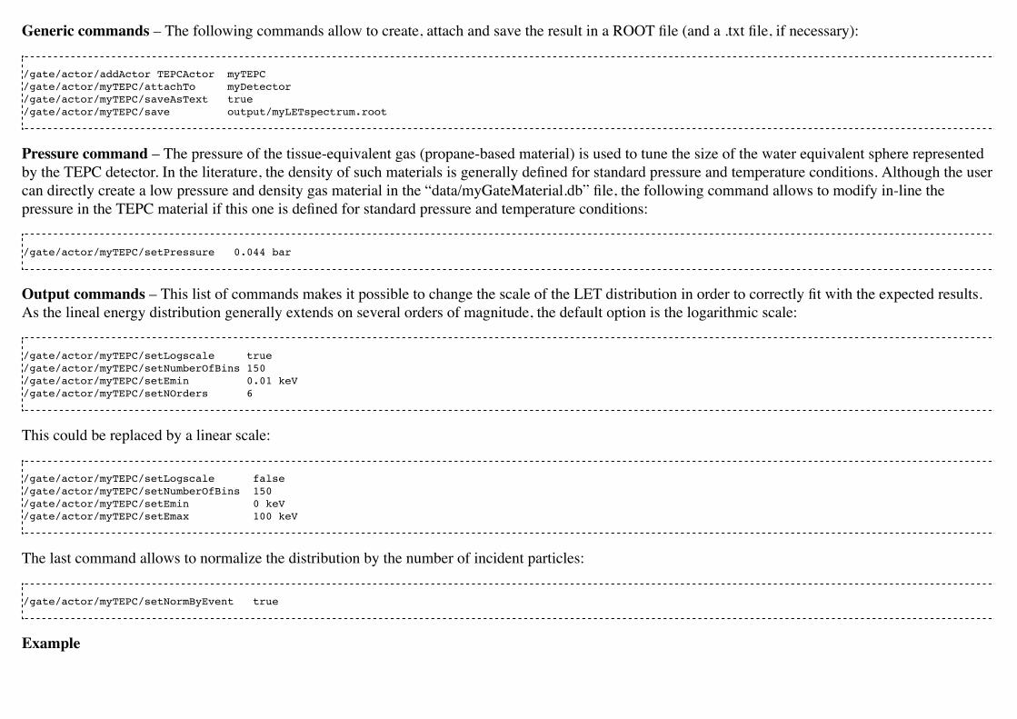
Generic commands – The following commands allow to create, attach and save the result in a ROOT file (and a .txt file, if necessary):

/gate/actor/addActor TEPCActor myTEPC/gate/actor/myTEPC/attachTo myDetector/gate/actor/myTEPC/saveAsText true/gate/actor/myTEPC/save output/myLETspectrum.root

Pressure command – The pressure of the tissue-equivalent gas (propane-based material) is used to tune the size of the water equivalent sphere representedby the TEPC detector. In the literature, the density of such materials is generally defined for standard pressure and temperature conditions. Although the usercan directly create a low pressure and density gas material in the “data/myGateMaterial.db” file, the following command allows to modify in-line thepressure in the TEPC material if this one is defined for standard pressure and temperature conditions:

/gate/actor/myTEPC/setPressure 0.044 bar

Output commands – This list of commands makes it possible to change the scale of the LET distribution in order to correctly fit with the expected results.As the lineal energy distribution generally extends on several orders of magnitude, the default option is the logarithmic scale:

/gate/actor/myTEPC/setLogscale true/gate/actor/myTEPC/setNumberOfBins 150/gate/actor/myTEPC/setEmin 0.01 keV/gate/actor/myTEPC/setNOrders 6

This could be replaced by a linear scale:

/gate/actor/myTEPC/setLogscale false/gate/actor/myTEPC/setNumberOfBins 150/gate/actor/myTEPC/setEmin 0 keV/gate/actor/myTEPC/setEmax 100 keV

The last command allows to normalize the distribution by the number of incident particles:

/gate/actor/myTEPC/setNormByEvent true

Example

An example of a TEPC actor use is provided in the example repository under dosimetry/TEPCActor(https://github.com/OpenGATE/GateContrib/tree/master/dosimetry/TEPCActor) folder. In this example, a TEPC detector is placed at different positions in awater tank and irradiated with a 155 MeV mono-energetic proton beam. This setup was used to validate the results against the TEPC measurementspublished by Kase et al. 2013. In this comparison, our key point was the optimization of the particle cuts and step limiters. Indeed, the lineal energydistribution at the micrometric scale is highly sensible to these two parameters. The particle cuts must be low enough to simulate any significant contributionin the lineal energy distribution and the step limiters must bec correctly tuned in order to avoid boundary effects on geometry elements, while keeping theglobal simulation time as low as possible. More information regarding the geometry and the physical parameters that were tested to obtain the final macrofiles are available in the example repository (TEPCactor.pdf(https://github.com/OpenGATE/GateContrib/blob/master/dosimetry/TEPCActor/TEPCactor.pdf)).

Phase Space Actor

This actor records information about particles entering the volume which the actor is attached to. They are two file types for the output: root file (.root) andIAEA file (.IAEAphsp and .IAEAheader). The name of the particle, the kinetic energy, the position along the three axes, the direction along the three axes,the weight are recorded. In a IAEA file, each particle is designated by an integer while the full name of the particle is recorded in the root file. Particles inIAEA files are limited to photons, electrons, positrons, neutrons and protons. The root file has two additional pieces of information: the name of the volumewhere the particle was produced and the name of the process which produced the particle. It is possible to disable some information in the phase space file :

/gate/actor/source/enableEkine false/gate/actor/source/enableXPosition false/gate/actor/source/enableYPosition false/gate/actor/source/enableZPosition false/gate/actor/source/enableXDirection false/gate/actor/source/enableYDirection false/gate/actor/source/enableZDirection false/gate/actor/source/enableProductionVolume false /gate/actor/source/enableProductionProcess false/gate/actor/source/enableParticleName false/gate/actor/source/enableWeight false

By default the frame used for the position and the direction of the particle is the frame of the world. To use the frame of the volume which the actor isattached to, the following command should be used :

/gate/actor/source/useVolumeFrame

/gate/actor/addActor PhaseSpaceActor MyActor/gate/actor/MyActor/save MyOutputFile.IAEAphsp

/gate/actor/MyActor/attachTo MyVolume/gate/actor/MyActor/enableProductionProcess false/gate/actor/MyActor/enableDirection false/gate/actor/MyActor/useVolumeFrame

By default, the phase space stores particles entering the volume. To store particles exiting the volume, the following command should be used :

/gate/actor/MyActor/storeOutgoingParticles true

To store all secondary particles created in the volume, use the command :

/gate/actor/MyActor/storeSecondaries true

Phase spaces built with all secondaries should not be used as source because some particles could be generated several times.

With ROOT files, to avoid very big files, it is possible to restrict the maximum size of the phase space. If a phase space reachs the maximum size, the filesis closed and a new file is created. The new file has the same name and a suffix is added. The suffix is the number of the file. For instance, instead of one fileof 10 GB, user may prefer 10 files of 1 GB. The value of the maximum size is not exactly the size of the file (value is the size of the TTree).

/gate/actor/MyActor/setMaxFileSize [Value] [Unit (B, kB, MB, GB)]

The source of the simulation could be a phase space. Gate read two types of phase space: root files and IAEA phase spaces. Both can be created withGate. However, Gate could read IAEA phase spaces created with others simulations.

/gate/source/addSource [Source name] phaseSpace

User can add several phase space files. All files should have the same informations about particles. The files are chained:

/gate/source/[Source name]/addPhaseSpaceFile [File name 1]/gate/source/[Source name]/addPhaseSpaceFile [File name 2]

If particles in the phase space are defined in the world frame, user has to used the command:

/gate/source/[Source name]/setPhaseSpaceInWorldFrame

If the particle type is not defined in the phase space file, user have to give the particle name. It is supposed that all particles have the same name:

/gate/source/[Source name]/setParticleType [Particle name]

If user have several phase space sources, each source have the same intensity. User can also choose to give at each source an intensity proportionnal to thenumber of particles in the files attach to the source:

/gate/source/[Source name]/useNbOfParticleAsIntensity true

For each run, if the number of events is higher than the number of particles in file, each particle is used several times with the same initial conditions.However, it is possible to rotate the particle position and direction around the z axis of the volume (make sure your phase space files have a rotationalsymmetry). The regular rotation is a rotation with a fixed angle :

where is the number of time the particle is used.

/gate/source/[Source name]/useRegularSymmetry

The random rotation is a rotation with a random angle.

/gate/source/[Source name]/useRandomSymmetry

By default, all particles in a phase space are used. The particles in the the phase space can be preselected in function of their position in the plan. Forinstance, a particle with a origin far from the collimator aperture is not useful and should be ignored. Particles in a cm-radius circle are selected. Theparticles outside the circle are ignored.

/gate/source/[Source name]/setRmax [r] [unit]

Thermal Actor

This actor records the optical photon deposited energy (photons absorbed by the tissue/material) in the volume which the actor is attached to. It alsoperforms the diffusion of the deposited energy. The output file format is a 3D matrix (voxelised image img/hdr). The Pennes bioheat model is used todescribe the diffusion of hear in biological perfused tissues. The Pennes equation is solved analytically via Fourier transformations and convolution theorem.The solution of the diffusion equation is equivalent to convolving the initial conditions (3D energy map) with a Gaussian with a standard deviation

, with t the diffusion time, the tissue thermal diffusivity. The blood perfusion term appears in the solution via an exponential function.

/gate/actor/addActor ThermalActor MyActor/gate/actor/MyActor/save 3DMap.hdr/gate/actor/MyActor/attachTo phantom/gate/actor/MyActor/stepHitType random/gate/actor/MyActor/setPosition 0. 0. 0. mm/gate/actor/MyActor/setVoxelSize 0.5 0.5 0.5 mm

Tissue thermal property : /gate/actor/MyActor/setThermalDiffusivity 0.32 mm2/s

Density and heat capacity should just be in the same unit for both blood and tissue. In the following example, the density is in kg/mm3 and the heat capacity in mJ kg/gate/actor/MyActor/setBloodDensity 1.06E-6/gate/actor/MyActor/setBloodHeatCapacity 3.6E6/gate/actor/MyActor/setTissueDensity 1.04E-6/gate/actor/MyActor/setTissueHeatCapacity 3.65E6/gate/actor/MyActor/setBloodPerfusionRate 0.004

During light illumination of a tissue, the thermal heat produced by the optical photons deposited energy does not accumulate locally in the tissue; it diffusesin biological tissues during illumination. This dynamic effect has been taken into account in the GATE code. The n seconds light illumination simulation issampled into p time frame 3D images by setting the simulation parameter setNumberOfTimeFrames to p. Each of the p sample images is diffused for aduration of [1, 2, ..., p-1] x n/p seconds. The final image illustrating the heat distribution in the tissues at the end of the illumination time is obtained byadding all diffused images to the last n/p seconds illumination image. This thermal energy (or heat) map will continue to diffuse after illumination by settingthe parameter setDiffusionTime to the value of interest. At a certain point in time after the initial temperature boost induced by nanoparticles, thetemperature of the tissues will go back to its initial value due to diffusion. This boundary condition is taken into account in a post processing-step of theGATE simulation.

/gate/actor/MyActor/setNumberOfTimeFrames 5/gate/actor/MyActor/setDiffusionTime 5 s

Merged Volume Actor

Since GATE v8.0, the user has to possibility to add a G4VSolid (or a analytical solid such as: box, cylinder, tessellated, sphere etc...) within a voxellizedvolume (defined by ImageRegularParametrisedVolume or ImageNestedParametrisedVolume).

To be done, the user needs an actor and MUST declare the volumes in a specific order. Here is a schematic procedure:

1. Declaring a volume containing the voxellized phantom AND the volume(s) to merge with the voxellized phantom2. Declaring the voxellized phantom3. Declaring all the analytical solid to add within the voxellized phantom

Here is a simple example:

# THE CONTAINER VOLUME/gate/world/daughters/name GlobalVol/gate/world/daughters/insert box/gate/GlobalVol/geometry/setXLength 90. mm/gate/GlobalVol/geometry/setYLength 90. mm/gate/GlobalVol/geometry/setZLength 90. mm/gate/GlobalVol/placement/setTranslation 0.0 0.0 0.0 mm/gate/GlobalVol/placement/setRotationAxis 1 0 0/gate/GlobalVol/placement/setRotationAngle 0 deg/gate/GlobalVol/setMaterial Air/gate/GlobalVol/vis/setColor cyan/gate/GlobalVol/describe

# THE VOXELLIZED PHANTOM/gate/GlobalVol/daughters/name PhantomTest/gate/GlobalVol/daughters/insert ImageRegularParametrisedVolume/gate/PhantomTest/geometry/setImage phantom_test_without_box.h33/gate/PhantomTest/geometry/setRangeToMaterialFile range.dat/gate/PhantomTest/placement/setTranslation 0. 0. 0. mm/gate/PhantomTest/placement/setRotationAxis 1 0 0/gate/PhantomTest/placement/setRotationAngle 0 deg/gate/PhantomTest/setSkipEqualMaterials 0

/gate/PhantomTest/describe

# 2 ANALYTICAL VOLUMES TO MERGE WITHIN VOXELLIZED PHANTOM# FIRST VOLUME/gate/GlobalVol/daughters/name BoxAir/gate/GlobalVol/daughters/insert box/gate/BoxAir/geometry/setXLength 10.0 mm/gate/BoxAir/geometry/setYLength 10.0 mm/gate/BoxAir/geometry/setZLength 10.0 mm/gate/BoxAir/placement/setTranslation -30.0 0.0 0.0 mm/gate/BoxAir/placement/setRotationAxis 1 0 0/gate/BoxAir/placement/setRotationAngle 0 deg/gate/BoxAir/setMaterial Air/gate/BoxAir/vis/setColor cyan/gate/BoxAir/describe# SECOND VOLUME/gate/GlobalVol/daughters/name BoxLung/gate/GlobalVol/daughters/insert box/gate/BoxLung/geometry/setXLength 10.0 mm/gate/BoxLung/geometry/setYLength 10.0 mm/gate/BoxLung/geometry/setZLength 10.0 mm/gate/BoxLung/placement/setTranslation -10.0 0.0 0.0 mm/gate/BoxLung/placement/setRotationAxis 1 0 0/gate/BoxLung/placement/setRotationAngle 0 deg/gate/BoxLung/setMaterial Lung/gate/BoxLung/vis/setColor red/gate/BoxLung/describe

The final step is to declare the actor. This actor MUST be the first actor declared in the GATE macro. This actor is like a navigator and its influence duringthe simulation is very important. Here is the declaration of the actor associated to the above example:

/gate/actor/addActor MergedVolumeActor mergedVol/gate/actor/mergedVol/attachTo GlobalVol/gate/actor/mergedVol/volumeToMerge BoxAir,BoxLung

For this actor, the order of the declared volume and the declared actor is very important. In the case of dosimetry, the user could add the dosimetry actor(after the MergedVolumeActor) to retrieve the energy deposit in the volume as follows:

/gate/actor/addActor DoseActor doseMeasurement/gate/actor/doseMeasurement/attachTo GlobalVol/gate/actor/doseMeasurement/save output/merged_volume.mhd/gate/actor/doseMeasurement/stepHitType random/gate/actor/doseMeasurement/setPosition 0 0 0 mm/gate/actor/doseMeasurement/setVoxelSize 0.5 0.5 0.5 mm

/gate/actor/doseMeasurement/setSize 90.5 90.5 90.5 mm/gate/actor/doseMeasurement/enableEdep true/gate/actor/doseMeasurement/enableUncertaintyEdep true/gate/actor/doseMeasurement/enableSquaredEdep true/gate/actor/doseMeasurement/enableDose false/gate/actor/doseMeasurement/enableUncertaintyDose false/gate/actor/doseMeasurement/enableSquaredDose false/gate/actor/doseMeasurement/enableNumberOfHits true

A complete example is provided here.

FiltersFilters are used to add selectrion criteria on actors. They are also used with reduction variance techniques. They are filters on particle type, particle ID,energy, direction....

Filter on particle type

With this filter it is possible to select particle with the name [Particle Name]

/gate/actor/[Actor Name]/addFilter particleFilter/gate/actor/[Actor Name]/particleFilter/addParticle [Particle Name]

User can select various particles. It is also possible to select particles which has a parent with the name [Particle Name]:

/gate/actor/[Actor Name]/addFilter particleFilter/gate/actor/[Actor Name]/particleFilter/addParentParticle [Particle Name]

For ions, user should use the Geant4 nomenclature (C12[0.0], c11[0.0]...). These names are different from those used for physics. To select all ions exceptalpha, deuton and triton, there is the key word 'GenericIon'.

Example: To kill electrons and positrons in the volume MyVolume

/gate/actor/addActor KillActor MyActor/gate/actor/MyActor/save MyOutputFile.txt/gate/actor/MyActor/attachTo MyVolume

/gate/actor/MyActor/addFilter particleFilter/gate/actor/MyActor/particleFilter/addParticle e-/gate/actor/MyActor/particleFilter/addParticle e+

Filter on particle ID

In an event, each track has an unique ID. The incident particle has an ID equal to 1. This filter select particles with the ID [Particle ID] or particles which hasa parent with the ID [Particle ID]. As for particle filter, user can select many IDs.

/gate/actor/[Actor Name]/addFilter IDFilter/gate/actor/[Actor Name]/IDFilter/selectID [Particle ID]

/gate/actor/[Actor Name]/addFilter IDFilter/gate/actor/[Actor Name]/IDFilter/selectParentID [Particle ID]

Example: To kill all particle exept the incident particle in the volume MyVolume (all particles are the children of the incident particle exept the incidentparticle itself)

/gate/actor/addActor KillActor MyActor/gate/actor/MyActor/save MyOutputFile.txt/gate/actor/MyActor/attachTo MyVolume/gate/actor/MyActor/addFilter IDFilter/gate/actor/MyActor/IDFilter/selectParentID 1

Filter on volume

This actor is especially useful for reduction variance techniques or for selections on daughter volumes.

Example: To kill particles in volume A and B, children of the volume MyVolume

/gate/actor/addActor KillActor MyActor/gate/actor/MyActor/save MyOutputFile.txt/gate/actor/MyActor/attachTo MyVolume/gate/actor/MyActor/addFilter volumeFilter/gate/actor/MyActor/volumeFilter/addVolume A/gate/actor/MyActor/volumeFilter/addVolume B

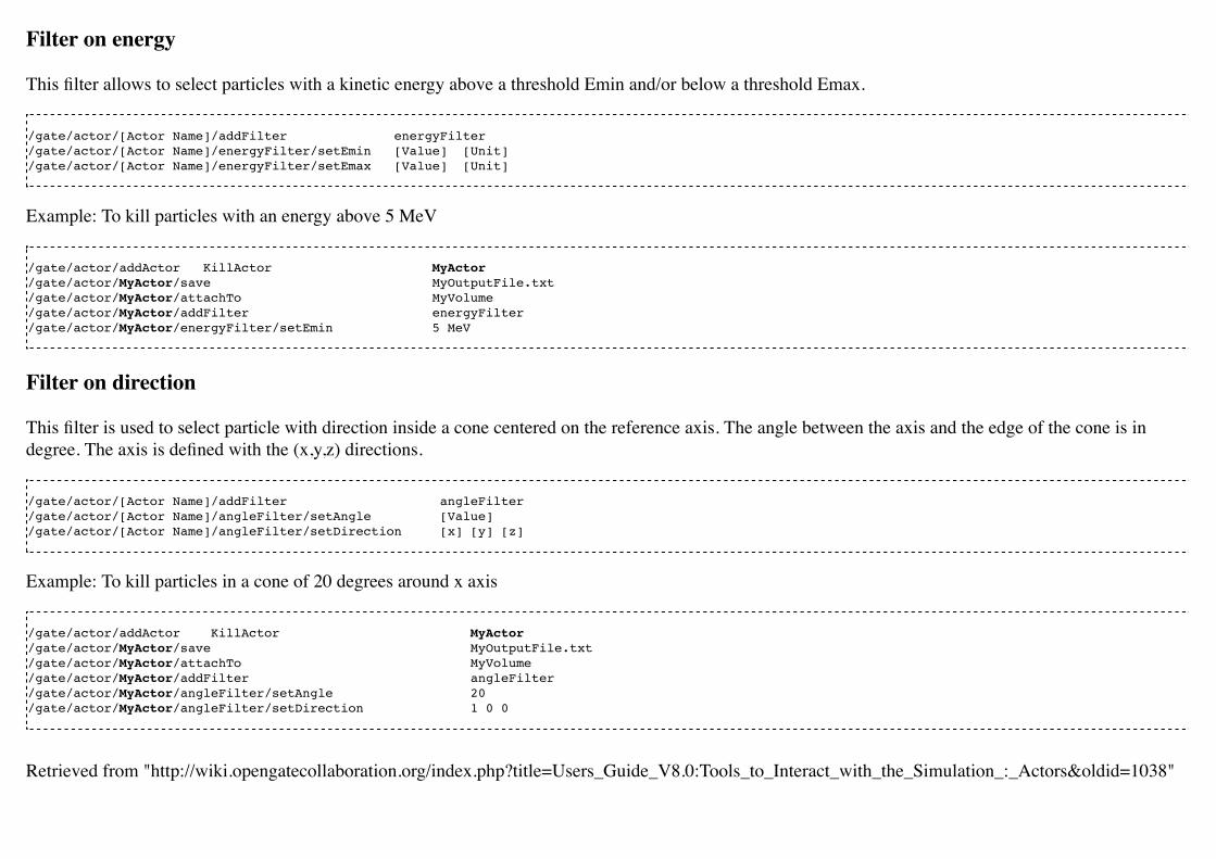
Filter on energy

This filter allows to select particles with a kinetic energy above a threshold Emin and/or below a threshold Emax.

/gate/actor/[Actor Name]/addFilter energyFilter/gate/actor/[Actor Name]/energyFilter/setEmin [Value] [Unit]/gate/actor/[Actor Name]/energyFilter/setEmax [Value] [Unit]

Example: To kill particles with an energy above 5 MeV

/gate/actor/addActor KillActor MyActor/gate/actor/MyActor/save MyOutputFile.txt/gate/actor/MyActor/attachTo MyVolume/gate/actor/MyActor/addFilter energyFilter/gate/actor/MyActor/energyFilter/setEmin 5 MeV

Filter on direction

This filter is used to select particle with direction inside a cone centered on the reference axis. The angle between the axis and the edge of the cone is indegree. The axis is defined with the (x,y,z) directions.

/gate/actor/[Actor Name]/addFilter angleFilter/gate/actor/[Actor Name]/angleFilter/setAngle [Value]/gate/actor/[Actor Name]/angleFilter/setDirection [x] [y] [z]

Example: To kill particles in a cone of 20 degrees around x axis

/gate/actor/addActor KillActor MyActor/gate/actor/MyActor/save MyOutputFile.txt/gate/actor/MyActor/attachTo MyVolume/gate/actor/MyActor/addFilter angleFilter/gate/actor/MyActor/angleFilter/setAngle 20/gate/actor/MyActor/angleFilter/setDirection 1 0 0

Retrieved from "http://wiki.opengatecollaboration.org/index.php?title=Users_Guide_V8.0:Tools_to_Interact_with_the_Simulation_:_Actors&oldid=1038"

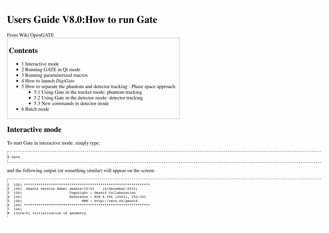
Users Guide V8.0:How to run GateFrom Wiki OpenGATE

Contents1 Interactive mode2 Running GATE in Qt mode3 Running parameterized macros4 How to launch DigiGate5 How to separate the phantom and detector tracking - Phase space approach

5.1 Using Gate in the tracker mode: phantom tracking5.2 Using Gate in the detector mode: detector tracking5.3 New commands in detector mode

6 Batch mode

Interactive modeTo start Gate in interactive mode, simply type:

$ Gate

and the following output (or something similar) will appear on the screen:

1 [G4] *************************************************************2 [G4] Geant4 version Name: geant4-10-03 (4-December-2015)3 [G4] Copyright : Geant4 Collaboration4 [G4] Reference : NIM A 506 (2003), 250-3035 [G4] WWW : http://cern.ch/geant46 [G4] *************************************************************7 [G4] 8 [Core-0] Initialization of geometry

9 [Core-0] Initialization of physics10 [Core-0] Initialization of actors11 [Core-0] 12 [Core-0] **********************************************************************13 [Core-0] GATE version name: gate_v8.0 14 [Core-0] Copyright : OpenGATE Collaboration 15 [Core-0] Reference : Phys. Med. Biol. 49 (2004) 4543-4561 16 [Core-0] Reference : Phys. Med. Biol. 56 (2011) 881-901 17 [Core-0] WWW : http://www.opengatecollaboration.org 18 [Core-0] **********************************************************************19 [Core-0] 20 [Core-0] You are using Geant4 version 10.3.021 Idle>

This output will vary depending on your Gate installation, that is which version of Geant4 software was installed and how it was installed.

Line 2 indicates the version of the Geant4 software in your installation. Lines 8-10 are initialization messages from Geant4. Line 13 indicates the version ofthe Gate software you are using. Finally, and if everything went right, then Gate outputs the interpreter command prompt (line 21). This means Gate is readyto read commands entered by the user.

If you are not yet familiar with Gate commands, you can get help by typing ls:

1 Idle> ls2 Command directory path : /3 Sub-directories :4 /control/ UI control commands.5 /units/ Available units.6 /process/ Process Table control commands.7 /gate/ GATE detector control.8 /particle/ Particle control commands.9 /geometry/ Geometry control commands.10 /tracking/ TrackingManager and SteppingManager control commands.11 /event/ EventManager control commands.12 /cuts/ Commands for G4VUserPhysicsList.13 /run/ Run control commands.14 /random/ Random number status control commands.15 /material/ Commands for materials16 /hits/ Sensitive detectors and Hits17 /vis/ Visualization commands.18 /digi/ DigitizerModule19 /gps/ ...Title not available...Commands :

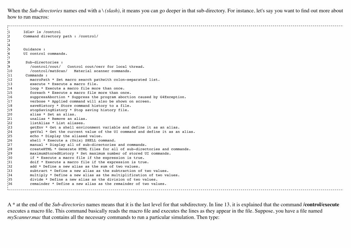
When the Sub-directories names end with a \ (slash), it means you can go deeper in that sub-directory. For instance, let's say you want to find out more abouthow to run macros:

1 Idle> ls /control2 Command directory path : /control/345 Guidance :6 UI control commands.78 Sub-directories : 9 /control/cout/ Control cout/cerr for local thread.10 /control/matScan/ Material scanner commands.11 Commands : 12 macroPath * Set macro search pathwith colon-separated list.13 execute * Execute a macro file.14 loop * Execute a macro file more than once.15 foreach * Execute a macro file more than once.16 suppressAbortion * Suppress the program abortion caused by G4Exception.17 verbose * Applied command will also be shown on screen.18 saveHistory * Store command history to a file.19 stopSavingHistory * Stop saving history file.20 alias * Set an alias.21 unalias * Remove an alias.22 listAlias * List aliases.23 getEnv * Get a shell environment variable and define it as an alias.24 getVal * Get the current value of the UI command and define it as an alias.25 echo * Display the aliased value.26 shell * Execute a (Unix) SHELL command.27 manual * Display all of sub-directories and commands.28 createHTML * Generate HTML files for all of sub-directories and commands.29 maximumStoredHistory * Set maximum number of stored UI commands.30 if * Execute a macro file if the expression is true.31 doif * Execute a macro file if the expression is true.32 add * Define a new alias as the sum of two values.33 subtract * Define a new alias as the subtraction of two values.34 multiply * Define a new alias as the multiplification of two values.35 divide * Define a new alias as the division of two values.36 remainder * Define a new alias as the remainder of two values.

A * at the end of the Sub-directories names means that it is the last level for that subdirectory. In line 13, it is explained that the command /control/executeexecutes a macro file. This command basically reads the macro file and executes the lines as they appear in the file. Suppose, you have a file namedmyScanner.mac that contains all the necessary commands to run a particular simulation. Then type:

1 Idle> /control/execute myScanner.mac

to run the macro file. The macro file myScanner.mac can contain additional /control/execute commands to run other macro files and so on. Gate will readand execute those files in the order in which they appear. Notice that /control/execute does not start a simulation (data acquisition), it simply reads thecommands and executes them. The command that starts the actual simulation is /gate/application/startDAQ, which is usually the last command found inyou macro files.

Depending on the level of verbosity that you have specified in your macro, you will see more or less messages about the simulation. If your simulationcontains visualization commands, you will see an OpenGL window appear with a beautiful picture of your scanner.

At the end of your simulation, the command line interpreter prompt will appear again. To exit the interpreter, type:

Idle> exitGraphics systems deleted.Visualization Manager deleting...

You can display the help typing this command:

$ Gate -h

and the following output (or something similar) will appear on the screen:

[Core-0] Gate command line help[Core-0] Usage: Gate [OPTION]... MACRO_FILE[Core-0] [Core-0] Mandatory arguments to long options are mandatory for short options too.[Core-0] -h, --help print the help[Core-0] -v, --version print the version[Core-0] -a, --param set alias. format is '[alias1,value1] [alias2,value2] ...'[Core-0] --d use the DigiMode[Core-0] --qt use the Qt visualization mode

Running GATE in Qt modeFirst you need to compile Geant4 with the variable 'GEANT4_USE_QT' setting to 'ON'. You can visualize the position of your system using the Qt mode.

Then you need to type the following command to your console:

$ Gate --qt

A window will display:

Afterwards you can launch your macro GATE using the 'Session:' section and typing /control/execute benchPET.mac. You will be able to visualize yoursystem in the viewer windows:

In order to use Qt you have to write this line in your GATE macro:

/vis/open OGLSQt

IMPORTANT!!!: Qt visualization mode is a visualization after the simulation. In fact you could zoom, translate, etc... only at the end of the simulation.

Running parameterized macrosIt is very common for users to run several simulations that differ in only a few parameters. For instance, a user might have designed a small animal PETscanner and would like to estimate its performance for five different crystal materials and three energy windows. In that case, the user does not need to writea complete set of macros for each simulation scenario. Instead, he can write parameterized macros. The actual values of the parameters are specified on thecommand line when running Gate or they can be defined with the interpreter.

For instance, suppose we want to parameterize the lower and upper level energy discriminators and the length of coincidence window. Here is thecorresponding macro command lines:

# D I G I T I Z E R1 /gate/digitizer/Singles/insert adder2 /gate/digitizer/Singles/insert readout3 /gate/digitizer/Singles/readout/setDepth 14 /gate/digitizer/Singles/insert blurring5 /gate/digitizer/Singles/blurring/setResolution 0.266 /gate/digitizer/Singles/blurring/setEnergyOfReference 511. keV7 /gate/digitizer/Singles/insert thresholder8 /gate/digitizer/Singles/thresholder/setThreshold {lld} keV9 /gate/digitizer/Singles/insert upholder10 /gate/digitizer/Singles/upholder/setUphold {uld} keV# C O I N C I D E N C E S O R T E R11 /gate/digitizer/Coincidences/setWindow {CoincWindow} ns

Lines 8, 10, and 11 define aliases for the lower level discriminator, the upper level discriminator, and the length of the coincidence window, respectively.

An alias is always specified between { and } (curled brackets) and it can consist of any set of characters.

To pass actual values to the macro file, you can run Gate, for instance, as follows:

$ Gate -a [CoincWindow,10] [lld,350] [uld,650]

It is worth emphasizing the following points about aliases:

The order of the aliases at the command line does not matter.Aliases are case sensitive, so [lld,350] is not the same as [LLD,350].All aliases in your macro file(s) must be defined when you run Gate. If some are undefined the simulation will fail.

How to launch DigiGateGATE offers an operating mode dedicated to digitizer optimization, known as DigiGate (see Users Guide V8.0:Digitizer and readout parameters). DigiGateworks by re-reading a previously generated ROOT hit-file.

The use of DigiGate consists of two steps.

In the first step, the simulation runs according to MacroTest.mac. This macro file should save the Hits data in the root output file with the namegate.root (which is the default name).In the second step, the digitizer modifications are made in MacroTest.mac (like a new module for the energy resolution, or a different dead-time...),and then the analysis is repeated by using the gate.root file as an input file for the program DigiGate. This is achieved by launching Gate with a '-d'option.

Gate < MacroTest.mac

-> a root output file is produced with Hits information.

-> the digitizer of MacroTest.mac is changed along with the name of the root output file.

Gate --d < MacroTest.mac

-> a new root output file is produced which incorporates the changes due to a different digitizer without having to repeat the particle generation and itspropagation.

How to separate the phantom and detector tracking - Phase space approach

To speed-up the simulation, it is possible to split and separate the particle tracking. This is a phase space approach with the possibility to store the phantomtracking particle history in a root file and to use it as an input file for the detector tracking.

Using Gate in the tracker mode: phantom tracking

Basically, as illustrated in the folder example_TrackerDetector, 3 major command lines are available to use the phantom tracker mode:

# Selection of the tracking mode#/gate/stepping/SetMode Tracker## Setting of the policy regarding the tracker mode#/gate/stepping/SetPolicy Option1/gate/stepping/SetPolicy Option2

The Option1 variable can be chosen from the following list:

StopOnPhantomBoundary (Default): the particles are tracked until the last hit before the phantom boundary ;StopAfterPhantomBoundary: the particles are traked until the first hit after phantom boundary ;KillTrackAndSecondaries: StopOnPhantomBoundary + no secondary production.

The Option2 variable may be chosen from:

KeepAll (Default): all particles (primary and secondary) are storedKeepOnlyPrimaries: only source particles are storedKeepOnlyPhotons: only photons are storedKeepOnlyElectrons: only electrons are stored

Two additional command line options are also available:

/gate/stepping/SetEnergyThreshold aThreshold keV

WIth this option, only particles reaching the phantom boundary with an energy greater than a threshold in energy of aThreshold (expressed in keV) will bestored.

/gate/stepping/SetTextOutput status

with a status flag set as On or Off. This command will print Tracks information in the PostStepInfo.txt file.

Finally the tracker mode acquisition will generate N root files named OutPutRoot_TrackerData_number.root. The base output name, which is OutPutRoot inthe case of this example, is chosen by the user with the usual output command line to set the file name:

/gate/output/root/setFileName OutPutRoot

Using Gate in the detector mode: detector tracking

During the tracker mode acquisition, N files are generated with the following name architecture:

OutPutRoot_TrackerData.rootOutPutRoot_TrackerData_1.rootOutPutRoot_TrackerData_2.root

...

OutPutRoot_TrackerData_(N-1).root

To use the Detector Mode, the user must select the mode and specify that N TrackerData files were generated during the tracker mode. All this can be doneusing the 2 following command lines:

/gate/stepping/SetMode Detector/gate/stepping/SetNumberOfTrackerDataFiles N

New commands in detector mode

In Detector Mode, we need to tell GATE that N TrackerData files were generated during tracker mode and we should use these command lines:

/gate/stepping/SetMode Detector/gate/stepping/SetNumberOfTrackerDataFiles N

Batch modeIt is possible to run a Gate simulation in batch mode, i.e. without the need to enter the interpreter and run the /control/execute and exit commands each time.

If you want to run simulations in batch mode, you can do so by typing the alias values or (--qt parameter) before the file name of the macro you want to run.For example,

$ Gate -a [CoincWindow,10] [lld,350] [uld,650] myScanner.mac

Or

$ Gate --qt myScanner.mac

In order to return to command prompt, the last line in myScanner.mac file must be

exit

This is very important, especially when you are running a series of simulations in sequence. If Gate does not find the exit command, it will return to the userinterface prompt and the rest of the simulations will not run.

It is recommended to redirect the terminal output of the simulation (listing of physics processes, sources, run time, etc.) by writing it to a text file instead ofprinting it in the terminal. This allows one to store the terminal output of each simulation for later viewing. For example,

$ Gate -a [CoincWindow,10] [lld,350] [uld,650] myScanner.mac > terminal_output.txt

The above command creates a file named terminal_output.txt and does not print to the terminal window.

When running multiple simulations simultaneously from the command line in batch mode, it is often desirable to have the process run in the background.This can be accomplished by inserting an ampersand "&" symbol at the end of the command. For example,

$ Gate -a [CoincWindow,10] [lld,350] [uld,650] myScanner.mac > terminal_output.txt &

It is recommended (although not compulsory) to avoid running visualization commands in batch mode.

Retrieved from "http://wiki.opengatecollaboration.org/index.php?title=Users_Guide_V8.0:How_to_run_Gate&oldid=917"


Users Guide V8.0:VisualizationFrom Wiki OpenGATE

Contents1 Introduction2 Important Hints3 Command Lines

3.1 Visualization with OpenGL4 Visualization of Images5 Immediate mode6 Stored mode

6.1 Visualization with DAWN6.2 Visualization with VRML6.3 Axes

IntroductionThe visualization options in GATE provide the same functionalities as provided in GEANT4. Most options in GEANT4 to visualize detector geometry,particle trajectories, tracking steps, etc. are also available in GATE. The graphics systems that can be selected in GATE are: DAWNFILE, VRMLFILE(versions 1 and 2) and OpenGL in stored and immediate mode, with OpenGL required as an external library. Most of the libraries are freely available.

Important HintsWhen loading digital images using OpenGL, the OpenGL Immediate-X viewer is recommended instead of the frequently used Stored-X viewer.

Using DAWN and VRMLVIEW, complicated geometries, like a huge number of crystals in a cylindrical PET system, may take very long to get rendered. Todecrease the file size and to speed up the visualization, the following option may be used:

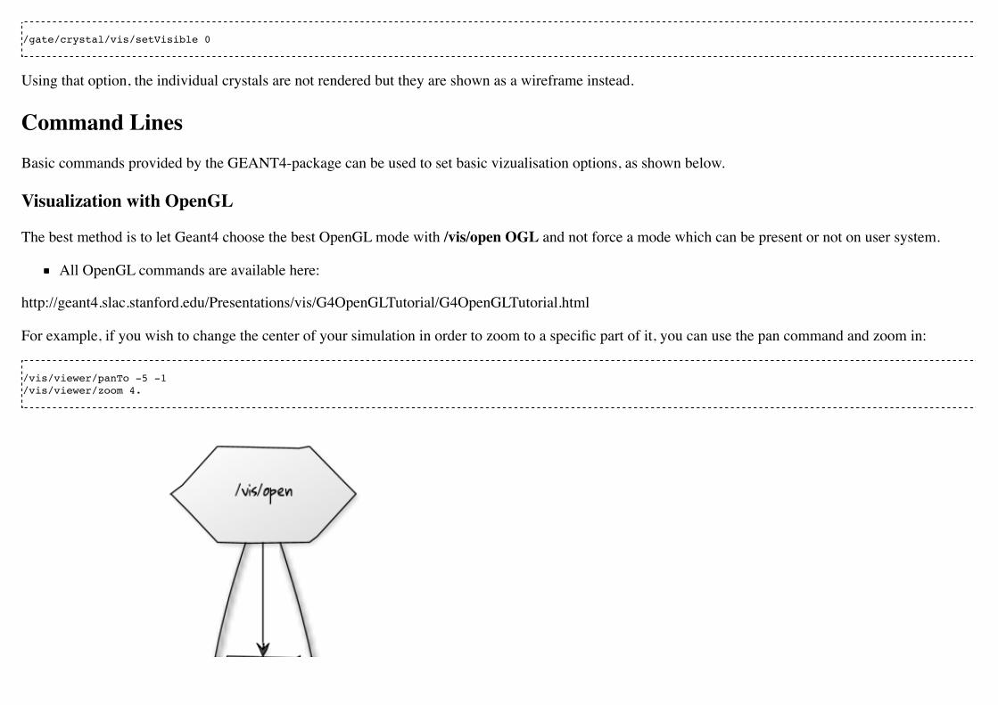
/gate/crystal/vis/setVisible 0

Using that option, the individual crystals are not rendered but they are shown as a wireframe instead.

Command LinesBasic commands provided by the GEANT4-package can be used to set basic vizualisation options, as shown below.

Visualization with OpenGL

The best method is to let Geant4 choose the best OpenGL mode with /vis/open OGL and not force a mode which can be present or not on user system.

All OpenGL commands are available here:

http://geant4.slac.stanford.edu/Presentations/vis/G4OpenGLTutorial/G4OpenGLTutorial.html

For example, if you wish to change the center of your simulation in order to zoom to a specific part of it, you can use the pan command and zoom in:

/vis/viewer/panTo -5 -1/vis/viewer/zoom 4.

# V I E W E R #/vis/open OGL

# define the zoom factor/vis/viewer/zoom 1.5# Set the viewing angle/vis/viewer/viewpointThetaPhi 5 60# Set the drawing style /vis/viewer/set/style surface# Tell the viewer to draw the volumes /vis/drawVolume# The trajectories for each run should be drawn together # don't store trajectories = 0; store trajectories = 1 /tracking/storeTrajectory 1# Requests viewer to refresh hits, tracks, etc., at end of event. # Or to accumulate drawings. Detector remains or is redrawn. /vis/scene/endOfEventAction accumulate

The following commands implement additional options relevant within GATE:

# draw object in WireFrame Mode/gate/block/vis/forceWireframe

or

# draw object to appear as a solid /gate/block/vis/forceSolid

# define object color/gate/block/vis/setColor blue

Instead of block as in the example here, objects like crystal, source, scanner can be assigned specific vizualization properties.

The "autoUpdate" capability has been removed since version 6.0.0 and manual geometry update has to be used instead. This can be done using the followingcommand at any moment in the GATE command prompt environment:

/gate/geometry/rebuild

Otherwise the complete geometry building is done when /gate/run/initialize command is given.

Visualization of Images

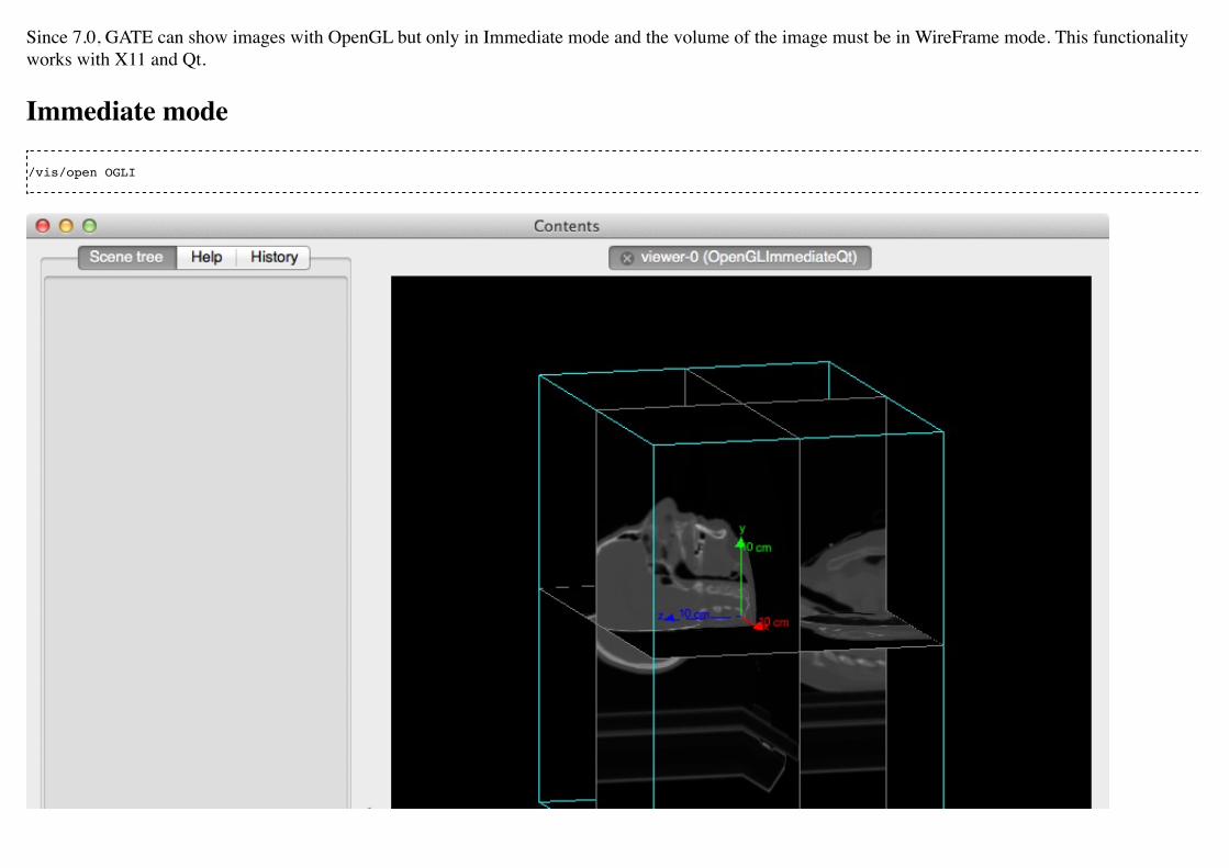
Since 7.0, GATE can show images with OpenGL but only in Immediate mode and the volume of the image must be in WireFrame mode. This functionalityworks with X11 and Qt.

Immediate mode

/vis/open OGLI

Stored mode/vis/open OGLS

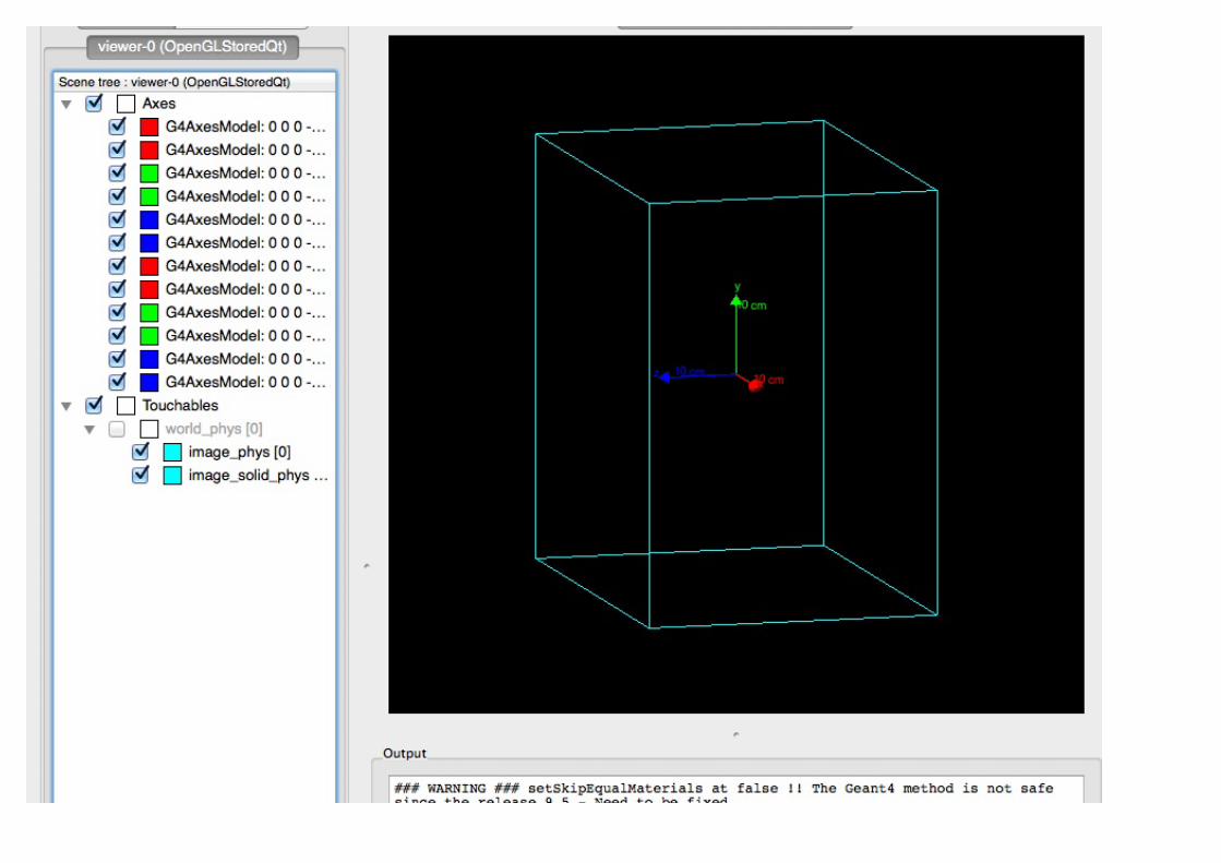
Visualization with DAWN

Instead of real-time visualization based on OpenGL, storing images in a file (mostly eps) for further processing might be useful. DAWN offers such options.

The package can be downloaded from the Internet and installed following the instruction given at http://geant4.kek.jp/tanaka/src/dawn_3_85e.taz

To use DAWN and DAWNFILE in your macro, a specific open command should be used, in replacement of the opening of OpenGL.

/vis/open DAWNFILE/vis/viewer/reset/vis/viewer/set/viewpointThetaPhi 30 0/vis/viewer/zoom 1.5/vis/drawVolume/tracking/storeTrajectory 1/vis/scene/endOfEventAction accumulate/vis/viewer/update /vis/viewer/refresh

Specific environment variables have to be set in your shell script to have access to DAWN inside GATE. For instance, in a C-shell:

if ( Xn == Xy ) thensetenv G4VIS_BUILD_DAWN_DRIVER 1

echo "On this machine the G4VIS_BUILD_DAWN_DRIVER= G4VIS_BUILD_DAWN_DRIVER"endif

and also

if ( Xn == Xy ) thensetenv G4VIS_USE_DAWN 1$echo "On this machine the G4VIS_USE_DAWN= G4VIS_USE_DAWN"endif

Visualization with VRML

Sometimes, it may be helpful to check a geometry setup by interactively manipulating the visualized scene. These features are offered by the optionVRML2FILE in connection with an appropriate viewer like vrmlview. Such a viewer can be freely downloaded from:http://www.sim.no/products/VRMLview/

A specific environment variable has to be set first:

setenv G4VRMLFILE_VIEWER vrmlview

For using this option in Gate, the following line has to be added to the macro instead of the corresponding OpenGL opening:

/vis/open VRML2FILE

Again, the environment variables have to be properly set (here C-schell example):

if [ Xn = Xy ] ;then G4VIS_BUILD_VRML_DRIVER=1 export G4VIS_BUILD_VRML_DRIVERecho "On this machine the G4VIS_BUILD_VRML_DRIVER=$G4VIS_BUILD_VRML_DRIVER"fi

if [ Xn = Xy ] ;then G4VIS_USE_VRML=1export G4VIS_USE_VRML

echo "On this machine the G4VIS_USE_VRML=$G4VIS_USE_VRML"fi

During processing in GATE, a file is written with the extension wrl.

Axes

Any position in the world is defined with respect to a three-axis system: X, Y and Z. These three axes can be seen in the display window using:

/vis/scene/add/axes

Retrieved from "http://wiki.opengatecollaboration.org/index.php?title=Users_Guide_V8.0:Visualization&oldid=258"


Users Guide V8.0:Defining a systemFrom Wiki OpenGATE

Contents1 Definition2 Choice of the system

2.1 Geometry constraints2.2 Constraints related to the simulation of the DAQ electronics

3 How to connect the geometry to a system4 Different types of systems

4.1 Scanner4.1.1 Description4.1.2 Use

4.2 CTscanner4.2.1 Use

4.3 CylindricalPET4.3.1 Description4.3.2 Use

4.4 CPET4.4.1 Description4.4.2 Use

4.5 Ecat4.5.1 Description4.5.2 Use

4.6 ecatAccel4.6.1 Description

4.6.1.1 Use4.7 OPET

4.7.1 Description4.7.1.1 Use

4.8 SPECTHead

4.8.1 Description4.8.2 Use4.8.3 Modelling the collimator4.8.4 Septal Penetration

4.9 OpticalSystem4.9.1 Description4.9.2 Use

5 How to define a multi-system detector5.1 Defining the systems:5.2 How to connect the geometry to the systems:5.3 Example of multi-system:5.4 Notes:

DefinitionA System is a key-concept of GATE. It provides a template of a predefined geometry to simulate a scanner. A system can be used to model several scannersshating the same general geometrical characteristics. It can be considered as sort of a template described by key components organized in a certain way, whatis called a tree level structure, each component having its own specific role or ordering.

For instance, in the cylindricalPET scanner system, the geometrical volumes containing crystals are grouped in matrices, themselves assembled insubmodules and modules. At the top level of this structure, the sectors composed of modules are repeated on a cylindrical surface to build up the wholedevice. Thus, a family of PET scanners obeying this structure can be described using this system, illustrated in figure 4.1, composed of volumes calledrsectors, modules, submodules, crystal and finaly (crystal) layer.

Different systems are available in GATE : scanner, SPECTHead, cylindricalPET, ecat, CPET, OPET and OpticalSystem, which can be used to simulatemost of the existing imaging devices.

Choice of the systemIt is possible to use GATE without using a system, but in that case, no information regarding particle interaction in the detector will be available. The reasonis that the volumes where the hits (interactions that occur inside the detector parts of the scanner, see Users Guide V7.2:Digitizer and readout parameters) arerecorded only for volumes belonging to a defined system (those volumes are declared as crystalSD, SD for sensitive detector, see Users Guide

Figure 4.1: Picture of a phantom and acylindricalPET system composed of 5 rsectors, 4modules (repeated along Z axis), 3 submodules(repeated along Y axis), 64 crystals (8 x 8) and 2layers (red and yellow)

V7.2:Attaching the sensitive detectors). When the user is only testing a scanner geometry, the use of a predefined system is not necessary. But if the userwants to record information related to the particle history inside the detector, the geometry has to be associated with a system. This section explains theelements and rules to associate a geometry with a system.

Geometry constraints

Except for the general system scanner, one should first take into account the geometrical shape of thedifferent components (gantry, sector, bucket, etc.) and also the shape of the crystal or the detectormaterial (e.g.scintillators).

Each level has to be assigned to a physical volume of the geometry. A level volume has to be fullyenclosed in the upper level volume.

The number of levels has to be set and must conform to the specifications listed in table 4.1. Thenumbering of different sensitive volumes is completely set by the choice of the system and conforms to aspecific output format.

The maximum number of components in each level depends on the output format since it can be limitedby the number of bits used for the numbering of the crystals. See Users Guide V7.2:Data output forfurther details.

Constraints related to the simulation of the DAQ electronics

Several points have to be considered when designing the simulation of the electronics cards. First, thewhole readout electronic components should be analyzed in order to define its main components. Thisconcerns not only the single channel simulation, with effects like thresholder response, but also thecrosstalk between different channels including the electronic or the optical crosstalk among componentsin a same level. For a PET scanner, the coincidence between two channels have to be simulated, basedon the single component simulations. In GATE, it is possible to introduce all these signal processingsteps through the digitizer modules (see Users Guide V7.2:Digitizer and readout parameters), operatingat different levels or depths, as shown in Table 4.2. The depth value is used here to tag a group of similar components operating at a certain level, whichcould be the scintillator block level (crystal with depth=5, or a group of crystal matrices with depth=1, depth values given in these examples refer to thecylindricalPET system).

To simulate the electronic processing consistenly with the system used to model the detector, the following procedure should be used:

Regroup the detector electronic components in different levels.

List the signal processing to be used for rach of the resulting groups (see adder, readout, dead time in Users Guide V7.2:Digitizer and readoutparameters),

Combine the signals coming from different volumes with, for example, the readout module for the signals summation of a volume, or the crosstalkand/or the coincidence between signals and coincidence.

NOTE : One or several crosstalk processing can be applied to components of different levels, for instance crosstalk between crystals, followed by crosstalkbetween modules. Such processing involves components at the same level. For PET scanners, coincidences are validated by testing the number difference inthe uppermost level (as defined as depth = 1 in table ). This test can reject accidental coincidence between adjacent logic structures. When the user builds ageometry, this logic organisation should correspond to the fisrt level of a system to use this coincidence sorting (see Users Guide V7.2:Digitizer and readoutparameters).

How to connect the geometry to a systemThe connection between the geometry and a system is performed in several steps:

The geometrical structure needs first to be defined, keeping in mind that it must fulfill some constraints, as described before.The system geometry has then to be introduced, or attached, in the simulation process with the ``attach'' command and a specific keyword argumentcorresponding to one level of the geometrical structure. The general macro line for this attachment is:

systems/SystemName/Level/attach UserVolumeName

where : SystemName is the specific name of the system (one of the entry in column 1), Level is the specific name of the level (see column 2),UserVolumeName is the name the user gave to a volume, according to the conventions of Users Guide V7.2:Defining a geometry.

Finally, the specific output corresponding to the system has to be defined for further data analysis (see Users Guide V7.2:Data output).

Table 4.1: Different systems available in GATE and their characteristics. In the second column are listed someof the keyword that are also used at in the macro (see also table 4.2 for a complete list). The shape in the thirdcolumn describe the mother volume, composed of “daughter” volumes as described in Chap. 3 : a box meansa box shaped mother volume containing an array of daughter boxes, a cylinder mother volumes will contains

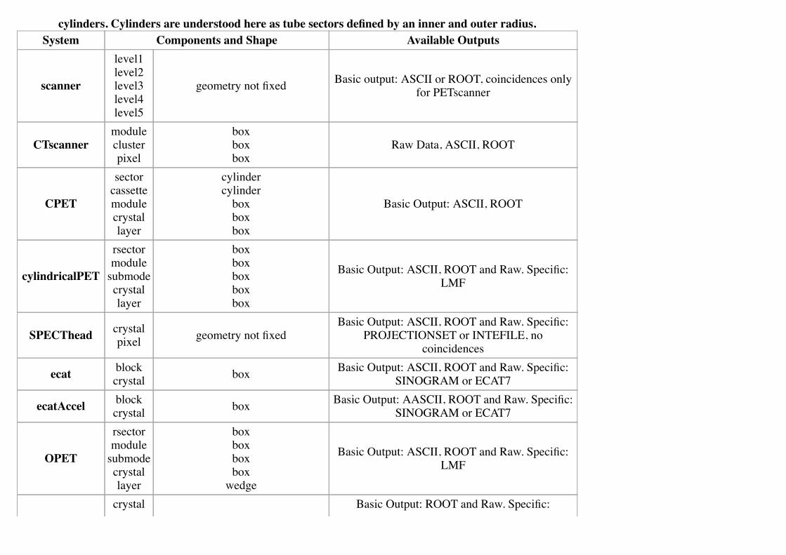
System Components and Shape Available Outputs

scanner

level1level2level3level4level5

geometry not fixed Basic output: ASCII or ROOT, coincidences onlyfor PETscanner

CTscannermoduleclusterpixel

boxboxbox

Raw Data, ASCII, ROOT

CPET

sectorcassettemodulecrystallayer

cylindercylinder

boxboxbox

Basic Output: ASCII, ROOT

cylindricalPET

rsectormodule

submodecrystallayer

boxboxboxboxbox

Basic Output: ASCII, ROOT and Raw. Specific:LMF

SPECThead crystalpixel geometry not fixed

Basic Output: ASCII, ROOT and Raw. Specific:PROJECTIONSET or INTEFILE, no

coincidences

ecat blockcrystal box Basic Output: ASCII, ROOT and Raw. Specific:

SINOGRAM or ECAT7

ecatAccel blockcrystal box Basic Output: AASCII, ROOT and Raw. Specific:

SINOGRAM or ECAT7

OPET

rsectormodule

submodecrystallayer

boxboxboxbox

wedge

Basic Output: ASCII, ROOT and Raw. Specific:LMF

crystal Basic Output: ROOT and Raw. Specific:

cylinders. Cylinders are understood here as tube sectors defined by an inner and outer radius.

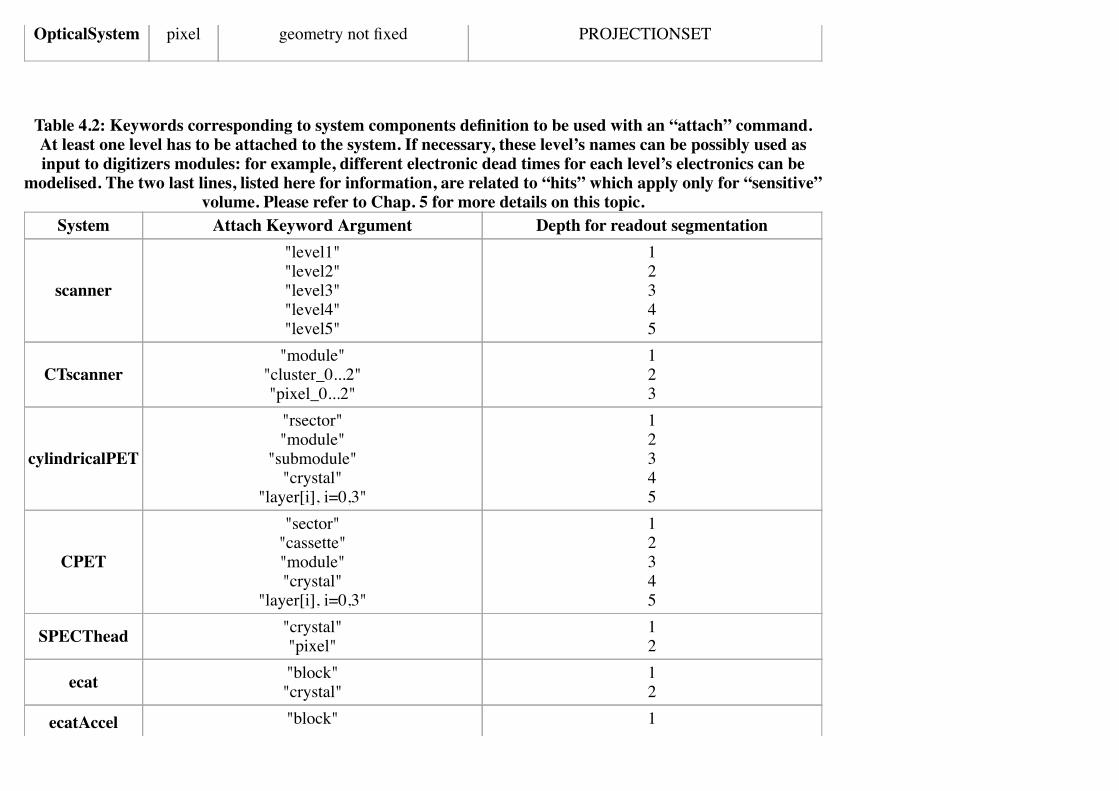
OpticalSystem pixel geometry not fixed PROJECTIONSET

System Attach Keyword Argument Depth for readout segmentation

scanner

"level1""level2""level3""level4""level5"

12345

CTscanner"module"

"cluster_0...2""pixel_0...2"

123

cylindricalPET

"rsector""module"

"submodule""crystal"

"layer[i], i=0,3"

12345

CPET

"sector""cassette""module""crystal"

"layer[i], i=0,3"

12345

SPECThead "crystal""pixel"

12

ecat "block""crystal"

12

ecatAccel "block" 1

Table 4.2: Keywords corresponding to system components definition to be used with an “attach” command.At least one level has to be attached to the system. If necessary, these level’s names can be possibly used asinput to digitizers modules: for example, different electronic dead times for each level’s electronics can be

modelised. The two last lines, listed here for information, are related to “hits” which apply only for “sensitive”volume. Please refer to Chap. 5 for more details on this topic.

"crystal" 2

OPET

"rsector""module"

"submodule""crystal"

"layer[i], i=0,7"

12345

OpticalSystem "crystal""pixel"

12

Different types of systems

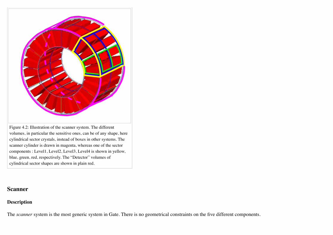
Figure 4.2: Illustration of the scanner system. The differentvolumes, in particular the sensitive ones, can be of any shape, herecylindrical sector crystals, instead of boxes in other systems. Thescanner cylinder is drawn in magenta, whereas one of the sectorcomponents : Level1, Level2, Level3, Level4 is shown in yellow,blue, green, red, respectively. The “Detector” volumes ofcylindrical sector shapes are shown in plain red.

Scanner

Description

The scanner system is the most generic system in Gate. There is no geometrical constraints on the five different components.

Use

Different shapes of the volumes inside the tree level can be choosen, among those listed in table 3.2

Figure 4.4 illustrates the kind of detector that can be simulated with this system without any geometry constraint. On the other hand, there is no specificoutput format associated with this system and information regarding the hits are only available in ROOT or ASCII format.

CTscanner

The CTscanner system allows you to simulate a simple CT scanner. It has three possible levels:

module component, that can be linearly repeated along the Y axis.cluster component, repeated inside the module, allowing you to simulate many kind of pixelspixel component, repeated inside the cluster. Raw data are the standard imageCT output to store the simulated CT projections and to produce it at eachtime slice. The image type is a float matrix (32-bits) of dimension given by the product of the number of pixels in X and Y, the content corresponds tothe number of counts per pixel per acquisition (time slice).

Three types of simulations are proposed to the user:

Complete simulation: The modules, the clusters, and the pixels are user defined. All volumes are created by Geant4 and the digitalization can bemade at the pixel level (level 3).

Fast simulation: Only the module level is defined. Geant4 creates one volume corresponding to the CT module (only one block possible) and thedigitalization is made by the output module. The number of pixels per module are given through the output module messenger. This mode is fastersince only one Geant4 volume is simulated, but obviously, only a rather approximated scanner response can be garanteed.

Complete simulation with a Variance Reduction Technique (VRT): In the same way as the complete simulation, the components (pixels, clusters,and modules) are user defined. Unlike the complete simulation, using Geant4 in the detector, the user handles the particle on the surface of the CTscanner. For more informations see the part below.

This variance reduction technique (VRT) has been developped with the aim to making the simulation time faster. Here are the successive steps of theimplementation:

Generation and Propagation of the particles through the World, then detection of those on the surface of the detector. The propagation of theparticles through the detector are 'killed', in order to handle ourself the detection and not by Geant4.

Computation of the mean free path (MFP) of the particle through the detector with the standard model (the compatibility with the low energy modelbeing not implemented yet)Computation of the path of the particle in the detector:

R being a distribution uniformly random number between 0 and 1

The user may perform this last step for each particle K times, in order to decrease the simulation time by avoiding a new generation and propagation of theparticle. However it has an influence on the variance of the output data. The following scheme shows the differences with a simulation with a without VRT:

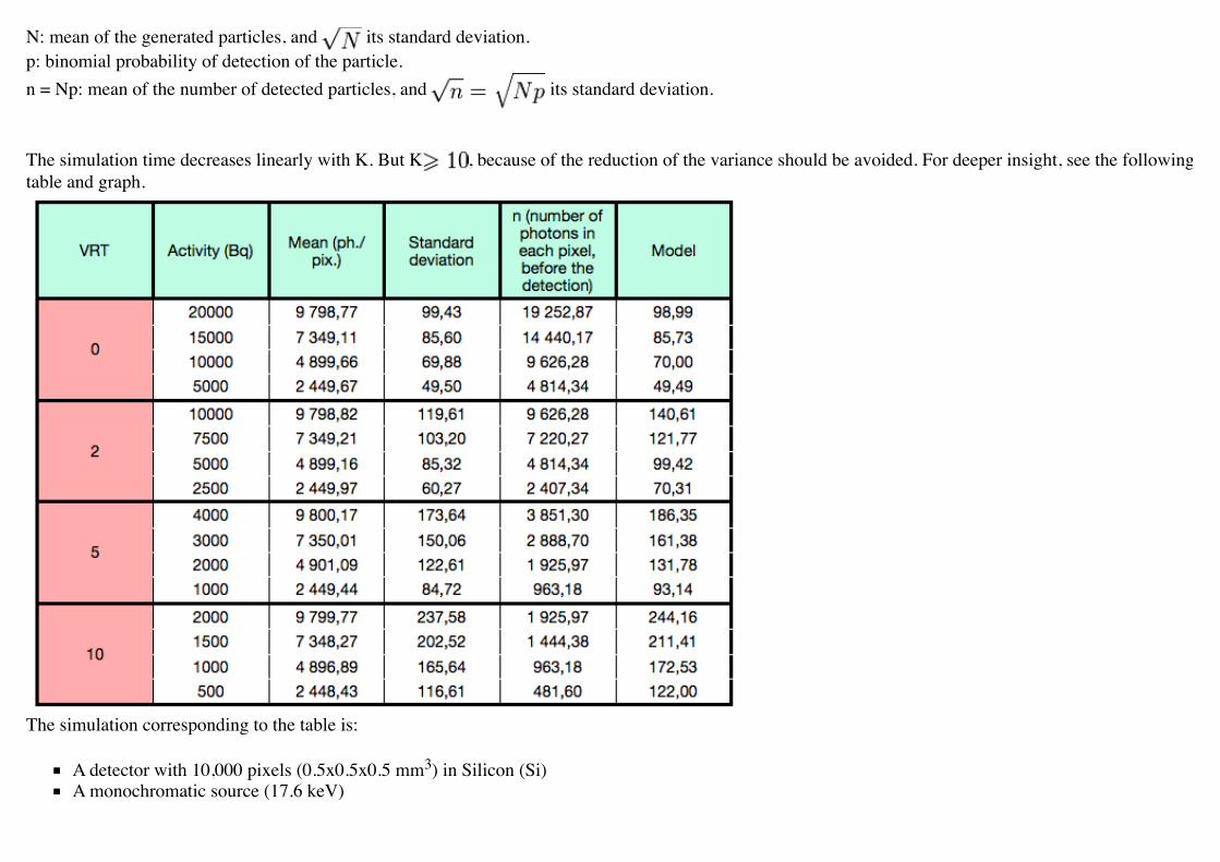
N: mean of the generated particles, and its standard deviation.p: binomial probability of detection of the particle.n = Np: mean of the number of detected particles, and its standard deviation.

The simulation time decreases linearly with K. But K , because of the reduction of the variance should be avoided. For deeper insight, see the followingtable and graph.

The simulation corresponding to the table is:

A detector with 10,000 pixels (0.5x0.5x0.5 mm3) in Silicon (Si)A monochromatic source (17.6 keV)

A time of exposition of 1 second

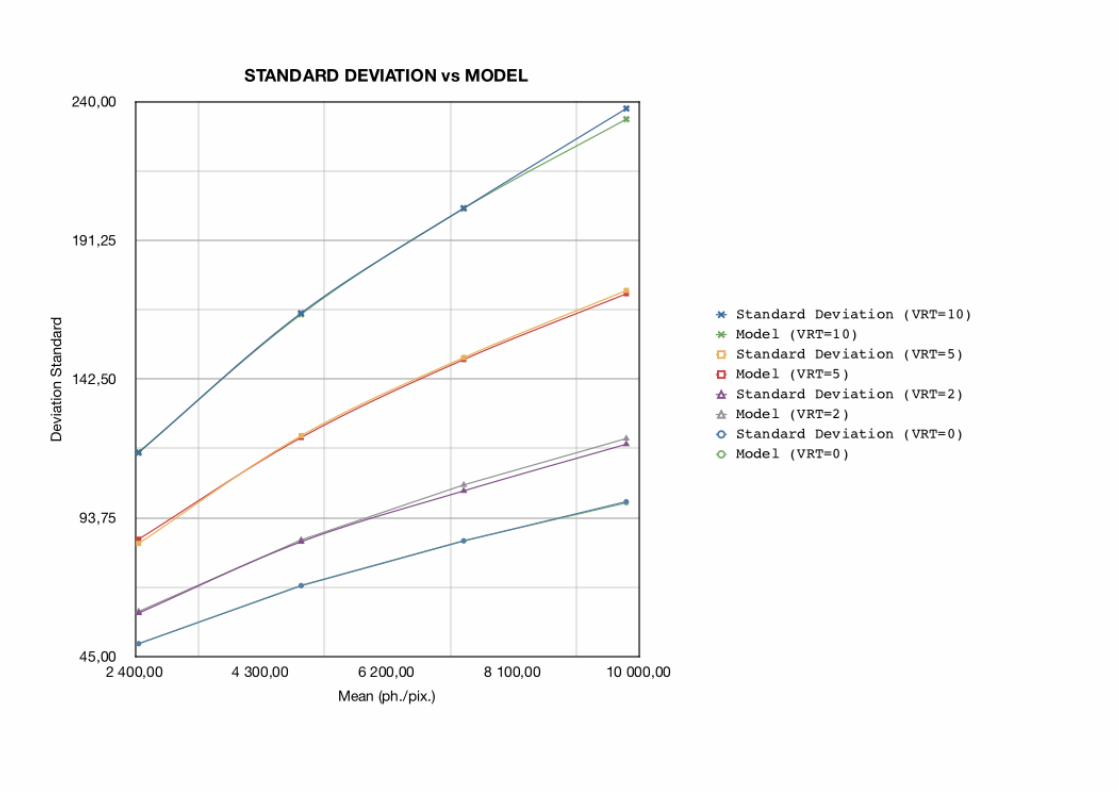
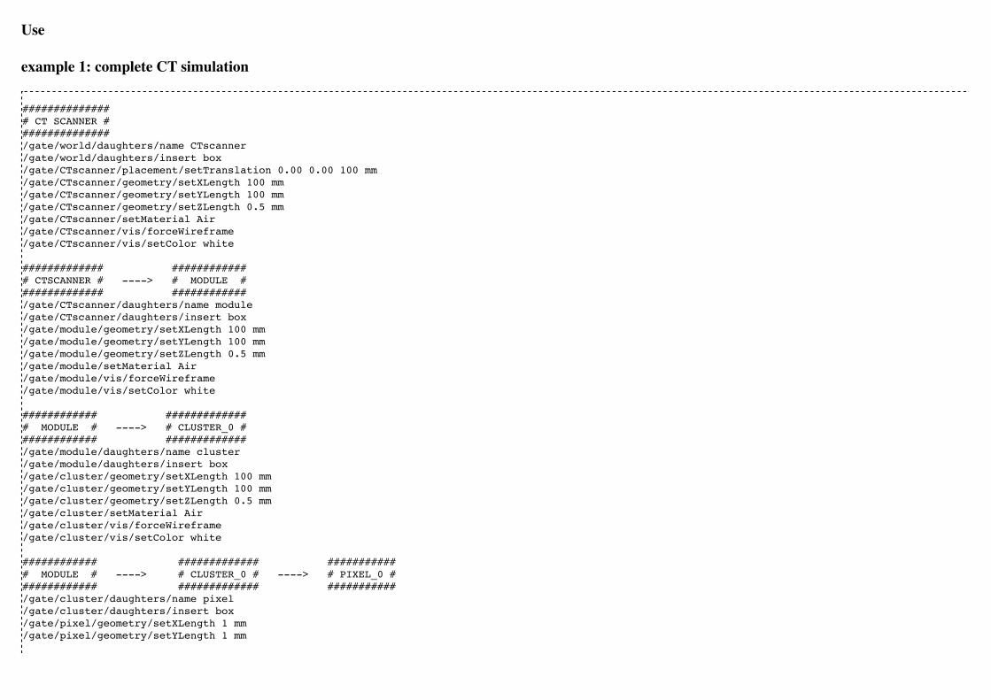
Use

example 1: complete CT simulation

############### CT SCANNER ############### /gate/world/daughters/name CTscanner/gate/world/daughters/insert box/gate/CTscanner/placement/setTranslation 0.00 0.00 100 mm/gate/CTscanner/geometry/setXLength 100 mm/gate/CTscanner/geometry/setYLength 100 mm/gate/CTscanner/geometry/setZLength 0.5 mm/gate/CTscanner/setMaterial Air/gate/CTscanner/vis/forceWireframe/gate/CTscanner/vis/setColor white

############# ############# CTSCANNER # ----> # MODULE ############## ############/gate/CTscanner/daughters/name module/gate/CTscanner/daughters/insert box/gate/module/geometry/setXLength 100 mm/gate/module/geometry/setYLength 100 mm/gate/module/geometry/setZLength 0.5 mm/gate/module/setMaterial Air/gate/module/vis/forceWireframe/gate/module/vis/setColor white

############ ############## MODULE # ----> # CLUSTER_0 ############# #############/gate/module/daughters/name cluster/gate/module/daughters/insert box/gate/cluster/geometry/setXLength 100 mm/gate/cluster/geometry/setYLength 100 mm/gate/cluster/geometry/setZLength 0.5 mm/gate/cluster/setMaterial Air/gate/cluster/vis/forceWireframe/gate/cluster/vis/setColor white

############ ############# ############ MODULE # ----> # CLUSTER_0 # ----> # PIXEL_0 ############# ############# ###########/gate/cluster/daughters/name pixel/gate/cluster/daughters/insert box/gate/pixel/geometry/setXLength 1 mm/gate/pixel/geometry/setYLength 1 mm

/gate/pixel/geometry/setZLength 1 mm/gate/pixel/setMaterial Silicon/gate/pixel/vis/setColor red

# REPEAT PIXEl_0/gate/pixel/repeaters/insert cubicArray/gate/pixel/cubicArray/setRepeatNumberX 100/gate/pixel/cubicArray/setRepeatNumberY 100/gate/pixel/cubicArray/setRepeatNumberZ 1/gate/pixel/cubicArray/setRepeatVector 1 1 0.0 mm/gate/pixel/cubicArray/autoCenter true

# ATTACH SYSTEM/gate/systems/CTscanner/module/attach module/gate/systems/CTscanner/cluster_0/attach cluster/gate/systems/CTscanner/pixel_0/attach pixel

# ATTACH LAYER/gate/pixel/attachCrystalSD

example 2: complete CT simulation with VRTIn the same way as the complete simulation, the difference is the output (K = 5)

/gate/output/imageCT/vrtFactor 5

Exemple 3 : Fast CT simulation

############### CT SCANNER ############### /gate/world/daughters/name CTscanner/gate/world/daughters/insert box/gate/CTscanner/placement/setTranslation 0.00 0.00 100 mm/gate/CTscanner/geometry/setXLength 1.00 mm/gate/CTscanner/geometry/setYLength 1.00 mm/gate/CTscanner/geometry/setZLength 0.50 mm/gate/CTscanner/setMaterial Air/gate/CTscanner/vis/forceWireframe/gate/CTscanner/vis/setColor white

############# ############# CTSCANNER # ----> # MODULE ############## ############/gate/CTscanner/daughters/name module/gate/CTscanner/daughters/insert box

/gate/module/geometry/setXLength 1. mm/gate/module/geometry/setYLength 1. mm/gate/module/geometry/setZLength 0.50 mm/gate/module/setMaterial Air/gate/module/vis/forceWireframe/gate/module/vis/setColor white

############ ############## MODULE # ----> # CLUSTER_0 ############# #############/gate/module/daughters/name cluster/gate/module/daughters/insert box/gate/cluster/geometry/setXLength 1. mm/gate/cluster/geometry/setYLength 1. mm/gate/cluster/geometry/setZLength 0.50 mm/gate/cluster/setMaterial Air/gate/cluster/vis/forceWireframe/gate/cluster/vis/setColor white

############ ############# ############ MODULE # ----> # CLUSTER_0 # ----> # PIXEL_0 ############# ############# ###########/gate/cluster/daughters/name pixel/gate/cluster/daughters/insert box/gate/pixel/geometry/setXLength 1. mm/gate/pixel/geometry/setYLength 1. mm/gate/pixel/geometry/setZLength 0.5 mm/gate/pixel/setMaterial Silicon/gate/pixel/vis/setColor red

# ATTACH SYSTEM /gate/systems/CTscanner/module/attach module/gate/systems/CTscanner/cluster_0/attach cluster/gate/systems/CTscanner/pixel_0/attach pixel

# ATTACH LAYER/gate/pixel/attachCrystalSD

/gate/output/imageCT/numFastPixelX 100/gate/output/imageCT/numFastPixelY 100/gate/output/imageCT/numFastPixelZ 1

CylindricalPET

Description

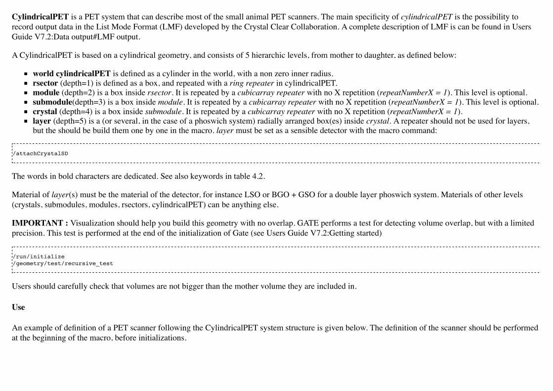
CylindricalPET is a PET system that can describe most of the small animal PET scanners. The main specificity of cylindricalPET is the possibility torecord output data in the List Mode Format (LMF) developed by the Crystal Clear Collaboration. A complete description of LMF is can be found in UsersGuide V7.2:Data output#LMF output.

A CylindricalPET is based on a cylindrical geometry, and consists of 5 hierarchic levels, from mother to daughter, as defined below:

world cylindricalPET is defined as a cylinder in the world, with a non zero inner radius.rsector (depth=1) is defined as a box, and repeated with a ring repeater in cylindricalPET.module (depth=2) is a box inside rsector. It is repeated by a cubicarray repeater with no X repetition (repeatNumberX = 1). This level is optional.submodule(depth=3) is a box inside module. It is repeated by a cubicarray repeater with no X repetition (repeatNumberX = 1). This level is optional.crystal (depth=4) is a box inside submodule. It is repeated by a cubicarray repeater with no X repetition (repeatNumberX = 1).layer (depth=5) is a (or several, in the case of a phoswich system) radially arranged box(es) inside crystal. A repeater should not be used for layers,but the should be build them one by one in the macro. layer must be set as a sensible detector with the macro command:

/attachCrystalSD

The words in bold characters are dedicated. See also keywords in table 4.2.

Material of layer(s) must be the material of the detector, for instance LSO or BGO + GSO for a double layer phoswich system. Materials of other levels(crystals, submodules, modules, rsectors, cylindricalPET) can be anything else.

IMPORTANT : Visualization should help you build this geometry with no overlap. GATE performs a test for detecting volume overlap, but with a limitedprecision. This test is performed at the end of the initialization of Gate (see Users Guide V7.2:Getting started)

/run/initialize/geometry/test/recursive_test

Users should carefully check that volumes are not bigger than the mother volume they are included in.

Use

An example of definition of a PET scanner following the CylindricalPET system structure is given below. The definition of the scanner should be performedat the beginning of the macro, before initializations.

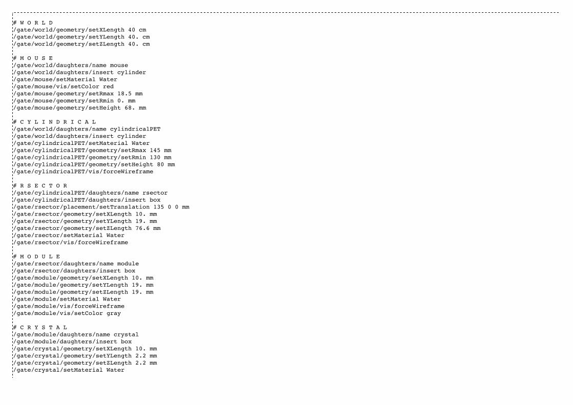
# W O R L D /gate/world/geometry/setXLength 40 cm /gate/world/geometry/setYLength 40. cm /gate/world/geometry/setZLength 40. cm

# M O U S E /gate/world/daughters/name mouse /gate/world/daughters/insert cylinder /gate/mouse/setMaterial Water /gate/mouse/vis/setColor red /gate/mouse/geometry/setRmax 18.5 mm /gate/mouse/geometry/setRmin 0. mm /gate/mouse/geometry/setHeight 68. mm

# C Y L I N D R I C A L /gate/world/daughters/name cylindricalPET /gate/world/daughters/insert cylinder /gate/cylindricalPET/setMaterial Water /gate/cylindricalPET/geometry/setRmax 145 mm /gate/cylindricalPET/geometry/setRmin 130 mm /gate/cylindricalPET/geometry/setHeight 80 mm /gate/cylindricalPET/vis/forceWireframe

# R S E C T O R /gate/cylindricalPET/daughters/name rsector /gate/cylindricalPET/daughters/insert box /gate/rsector/placement/setTranslation 135 0 0 mm /gate/rsector/geometry/setXLength 10. mm /gate/rsector/geometry/setYLength 19. mm /gate/rsector/geometry/setZLength 76.6 mm /gate/rsector/setMaterial Water /gate/rsector/vis/forceWireframe

# M O D U L E /gate/rsector/daughters/name module /gate/rsector/daughters/insert box /gate/module/geometry/setXLength 10. mm /gate/module/geometry/setYLength 19. mm /gate/module/geometry/setZLength 19. mm /gate/module/setMaterial Water /gate/module/vis/forceWireframe /gate/module/vis/setColor gray

# C R Y S T A L /gate/module/daughters/name crystal /gate/module/daughters/insert box /gate/crystal/geometry/setXLength 10. mm /gate/crystal/geometry/setYLength 2.2 mm /gate/crystal/geometry/setZLength 2.2 mm /gate/crystal/setMaterial Water

/gate/crystal/vis/forceWireframe /gate/crystal/vis/setColor magenta

# L A Y E R /gate/crystal/daughters/name LSO /gate/crystal/daughters/insert box /gate/LSO/geometry/setXLength 10. mm /gate/LSO/geometry/setYLength 2.2 mm /gate/LSO/geometry/setZLength 2.2 mm /gate/LSO/placement/setTranslation 0 0 0 mm /gate/LSO/setMaterial LSO /gate/LSO/vis/setColor yellow

# R E P E A T C R Y S T A L /gate/crystal/repeaters/insert cubicArray /gate/crystal/cubicArray/setRepeatNumberX 1 /gate/crystal/cubicArray/setRepeatNumberY 8 /gate/crystal/cubicArray/setRepeatNumberZ 8 /gate/crystal/cubicArray/setRepeatVector 10. 2.4 2.4 mm

# R E P E A T M O D U L E /gate/module/repeaters/insert cubicArray /gate/module/cubicArray/setRepeatNumberZ 4 /gate/module/cubicArray/setRepeatVector 0. 0. 19.2 mm

# R E P E A T R S E C T O R /gate/rsector/repeaters/insert ring /gate/rsector/ring/setRepeatNumber 42

# A T T A C H S Y S T E M /gate/systems/cylindricalPET/rsector/attach rsector /gate/systems/cylindricalPET/module/attach module /gate/systems/cylindricalPET/crystal/attach crystal /gate/systems/cylindricalPET/layer0/attach LSO

# A T T A C H L A Y E R SD /gate/LSO/attachCrystalSD /gate/mouse/attachPhantomSD

CPET

This system was defined for the simulation of a CPET-like scanner (C-PET Plus, Philips Medical Systems, the Netherlands), with one ring of NaI crystalwith a curved shape. For this scanner, a single level in addition to the system level is enough to describe the volume hierarchy.

Description

This system has the particularity to have cylindrical shaped sector components, based on the cylinder shape (see figure 4.3 and Users Guide V7.2:Defining ageometry for definitions), whereas these components are generally boxes in other systems.

Figure: 4.3: Definition of a CPETsector volume. This system allowsone to define sectors with acylindrical shape instead of sectorswith a box shape,like in other PETsystems

Use

Described below is an example of code appropriate for modeling a one ring scanner of NaI crystal with a curved shape.

# BASE = CPET SYSTEM /gate/world/daughters/name CPET /gate/world/daughters/insert cylinder /gate/CPET/setMaterial Air /gate/CPET/geometry/setRmax 60 cm /gate/CPET/geometry/setRmin 0.0 cm /gate/CPET/geometry/setHeight 35.0 cm /gate/CPET/vis/forceWireframe

# FIRST LEVEL = CRYSTAL /gate/CPET/daughters/name crystal /gate/CPET/daughters/insert cylinder /gate/crystal/geometry/setRmax 47.5 cm

Figure 4.4: One NaI crystal with a curved shape

/gate/crystal/geometry/setRmin 45.0 cm /gate/crystal/geometry/setHeight 25.6 cm /gate/crystal/geometry/setPhiStart 0 deg /gate/crystal/geometry/setDeltaPhi 60 deg

# REPEAT THE CURVE SECTOR INTO THE WHOLE RING /gate/crystal/repeaters/insert ring /gate/crystal/ring/setRepeatNumber 6

# CRYSTAL VOLUME IS MADE OF NAI /gate/crystal/setMaterial NaI /gate/crystal/vis/setColor green

The object crystal is then attached to its corresponding component in the CPET system (level 1 : the sector level for CPET system - see previous section fordetails).

/gate/systems/CPET/sector/attach crystal

The crystals are set as sensitive detectors (see Users Guide V7.2:Attaching the sensitive detectors#ThecrystalSD).

/gate/crystal/attachCrystalSD

The digitizer part (see Users Guide V7.2:Digitizer and readout parameters#Digitizer modules) is made ofthe adder module and some blurring module (see Users Guide V7.2:Digitizer and readout parameters).

Ecat

Description

The ecat system is a simplified version of cylindricalPET and was named ecat because it is appropriate formodelling PET scanners from the ECAT family, from CPS Innovations (Knoxville, TN, U.S.A.). Such scanners are based on the block detector principle,consisting in an array of crystals, typically 8 x 8 read by few photomultipliers, typically 4. The blocks are organized along an annular geometry to yieldmulti-ring detectors.

An example of macro with an ecat definition is provided in:

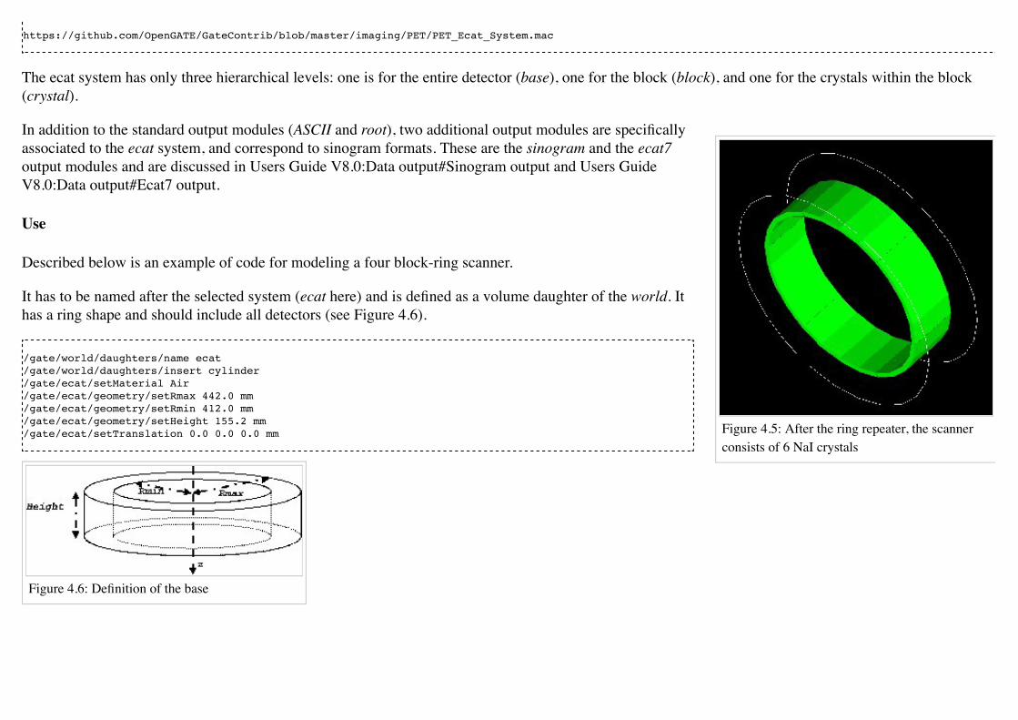
Figure 4.5: After the ring repeater, the scannerconsists of 6 NaI crystals

https://github.com/OpenGATE/GateContrib/blob/master/imaging/PET/PET_Ecat_System.mac

The ecat system has only three hierarchical levels: one is for the entire detector (base), one for the block (block), and one for the crystals within the block(crystal).

In addition to the standard output modules (ASCII and root), two additional output modules are specificallyassociated to the ecat system, and correspond to sinogram formats. These are the sinogram and the ecat7output modules and are discussed in Users Guide V8.0:Data output#Sinogram output and Users GuideV8.0:Data output#Ecat7 output.

Use

Described below is an example of code for modeling a four block-ring scanner.

It has to be named after the selected system (ecat here) and is defined as a volume daughter of the world. Ithas a ring shape and should include all detectors (see Figure 4.6).

/gate/world/daughters/name ecat /gate/world/daughters/insert cylinder /gate/ecat/setMaterial Air /gate/ecat/geometry/setRmax 442.0 mm /gate/ecat/geometry/setRmin 412.0 mm /gate/ecat/geometry/setHeight 155.2 mm /gate/ecat/setTranslation 0.0 0.0 0.0 mm

Figure 4.6: Definition of the base

Figure 4.7: Definition of the block

The following commands set the size and the position of the first block within the base ecat. It is a rectangular parallelepiped and should include all crystalswithin a block. For a multiple block-ring system centered axially on the base ecat, the axial position of this first block should be set to zero (see Figure 4.7).

/gate/ecat/daughters/name block /gate/ecat/daughters/insert box /gate/block/placement/setTranslation 427.0 0.0 0.0 mm /gate/block/geometry/setXLength 30.0 mm /gate/block/geometry/setYLength 35.8 mm /gate/block/geometry/setZLength 38.7 mm /gate/block/setMaterial Air

Figure 4.8: Definition of the crystal

The next commands set the size and the position of the first crystal within the block. For a crystal array centered on the block, the position of this first crystalshould be at the center of the block (see Figure 4.8).

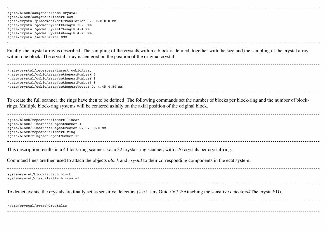
/gate/block/daughters/name crystal /gate/block/daughters/insert box /gate/crystal/placement/setTranslation 0.0 0.0 0.0 mm /gate/crystal/geometry/setXLength 30.0 mm /gate/crystal/geometry/setYLength 4.4 mm /gate/crystal/geometry/setZLength 4.75 mm /gate/crystal/setMaterial BGO

Finally, the crystal array is described. The sampling of the crystals within a block is defined, together with the size and the sampling of the crystal arraywithin one block. The crystal array is centered on the position of the original crystal.

/gate/crystal/repeaters/insert cubicArray /gate/crystal/cubicArray/setRepeatNumberX 1 /gate/crystal/cubicArray/setRepeatNumberY 8 /gate/crystal/cubicArray/setRepeatNumberZ 8 /gate/crystal/cubicArray/setRepeatVector 0. 4.45 4.80 mm

To create the full scanner, the rings have then to be defined. The following commands set the number of blocks per block-ring and the number of block-rings. Multiple block-ring systems will be centered axially on the axial position of the original block.

/gate/block/repeaters/insert linear /gate/block/linear/setRepeatNumber 4 /gate/block/linear/setRepeatVector 0. 0. 38.8 mm /gate/block/repeaters/insert ring /gate/block/ring/setRepeatNumber 72

This description results in a 4 block-ring scanner, i.e. a 32 crystal-ring scanner, with 576 crystals per crystal-ring.

Command lines are then used to attach the objects block and crystal to their corresponding components in the ecat system.

systems/ecat/block/attach block systems/ecat/crystal/attach crystal

To detect events, the crystals are finally set as sensitive detectors (see Users Guide V7.2:Attaching the sensitive detectors#The crystalSD).


The digitizer part (see Users Guide V7.2:Digitizer and readout parameters#Digitizer modules) can be the same as for the cylindricalPET system.

ecatAccel

Description

The ecatAccel system was introduced to model a new PET scanner family ECAT ACCEL (from CPS Innovations, Knoxville, TN, U.S.A.). The ecatAccelsystem differs from the ecat system by its geometrical shape : the detection blocks are arranged along a spherical ring whereas they are arranged alongannular rings for the ecat system. As data processing and output format are highly dependent on the scanner geometry, it was necessary to introduce a newsystem even though it has many common features with the ecat system. The same hierarchical levels (base, block and crystal) as for the ecat system are usedto describe the geometry of the ecatAccel system, and the same standard output modules (ASCII and root) and specific outputs (sinogram and ecat7) are alsoavailable. Please refer to [Users Guide V7.2:Data output#Sinogram output]] and Users Guide V7.2:Data output#Ecat7 output for further information onsinogram and ecat7 outputs for the ecatAccel system.

Use

Described below is an example of code for modeling the ACCEL PET scanner of the BIOGRAPH-LSO (SIEMENS - CTI) PET-CT scanner.

The scanner is named after the selected system (ecatAccel here) and is defined as a volume daughter of the world. As for the ecat system, it has a ring shapeand should include all detectors (see Figure 4.6). For the BIOGRAPH, it can be described as follows:

The base is described:

/gate/world/daughters/name ecatAccel /gate/world/daughters/insert cylinder /gate/ecatAccel/setMaterial Air /gate/ecatAccel/geometry/setRmax 437.0 mm /gate/ecatAccel/geometry/setRmin 412.0 mm /gate/ecatAccel/geometry/setHeight 162. mm /gate/ecatAccel/setTranslation 0.0 0.0 0.0 mm

The block is then described: the size and the position of the first block are set within the base ecatAccel. As for the ecat system, it is a rectangularparallelepiped and should include all crystals within a block. For a multiple block-ring system centered axially on the base ecatAccel, the axial position ofthis first block should be set to zero.

/gate/ecatAccel/daughters/name block

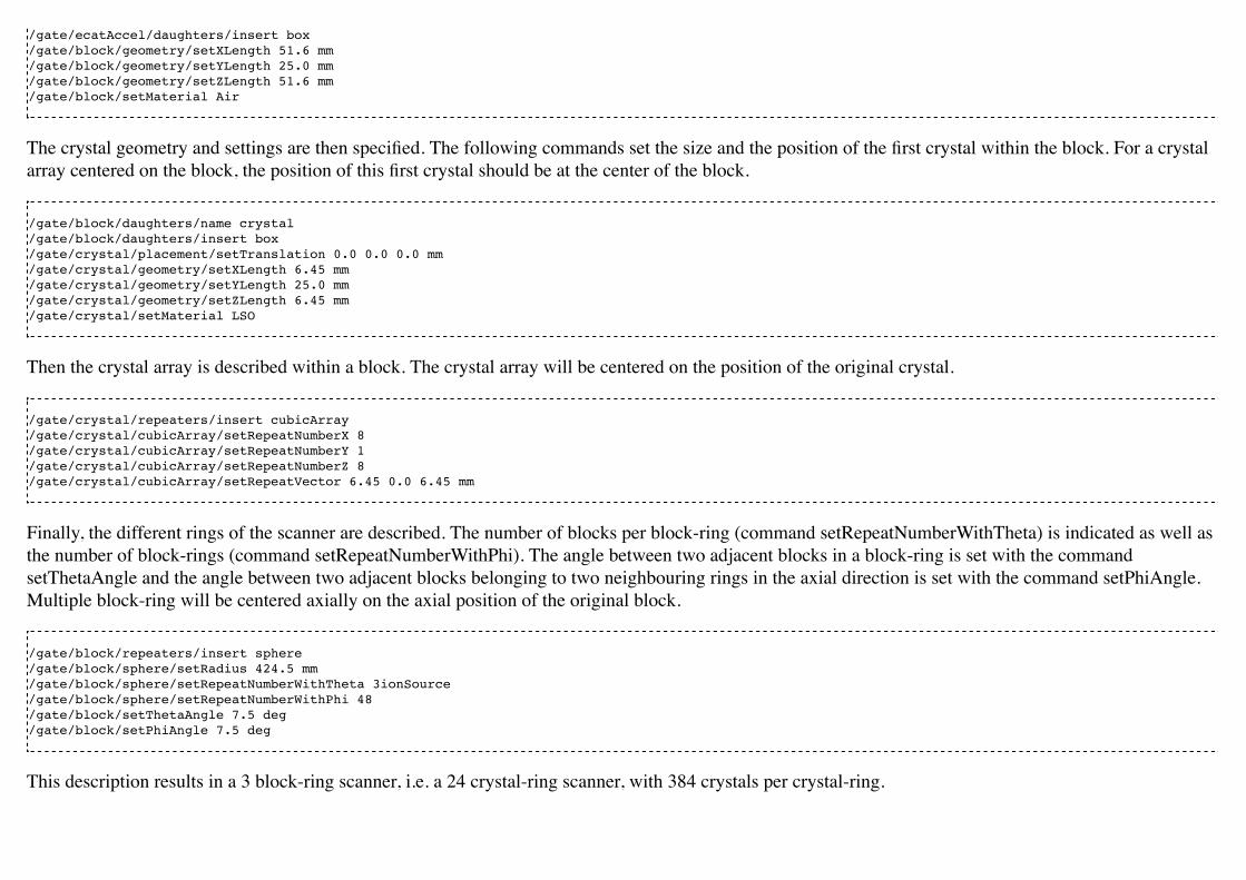
/gate/ecatAccel/daughters/insert box /gate/block/geometry/setXLength 51.6 mm /gate/block/geometry/setYLength 25.0 mm /gate/block/geometry/setZLength 51.6 mm /gate/block/setMaterial Air

The crystal geometry and settings are then specified. The following commands set the size and the position of the first crystal within the block. For a crystalarray centered on the block, the position of this first crystal should be at the center of the block.

/gate/block/daughters/name crystal /gate/block/daughters/insert box /gate/crystal/placement/setTranslation 0.0 0.0 0.0 mm /gate/crystal/geometry/setXLength 6.45 mm /gate/crystal/geometry/setYLength 25.0 mm /gate/crystal/geometry/setZLength 6.45 mm /gate/crystal/setMaterial LSO

Then the crystal array is described within a block. The crystal array will be centered on the position of the original crystal.

/gate/crystal/repeaters/insert cubicArray /gate/crystal/cubicArray/setRepeatNumberX 8 /gate/crystal/cubicArray/setRepeatNumberY 1 /gate/crystal/cubicArray/setRepeatNumberZ 8 /gate/crystal/cubicArray/setRepeatVector 6.45 0.0 6.45 mm

Finally, the different rings of the scanner are described. The number of blocks per block-ring (command setRepeatNumberWithTheta) is indicated as well asthe number of block-rings (command setRepeatNumberWithPhi). The angle between two adjacent blocks in a block-ring is set with the commandsetThetaAngle and the angle between two adjacent blocks belonging to two neighbouring rings in the axial direction is set with the command setPhiAngle.Multiple block-ring will be centered axially on the axial position of the original block.

/gate/block/repeaters/insert sphere /gate/block/sphere/setRadius 424.5 mm /gate/block/sphere/setRepeatNumberWithTheta 3ionSource /gate/block/sphere/setRepeatNumberWithPhi 48 /gate/block/setThetaAngle 7.5 deg /gate/block/setPhiAngle 7.5 deg

This description results in a 3 block-ring scanner, i.e. a 24 crystal-ring scanner, with 384 crystals per crystal-ring.

The objects block and crystal are attached to their corresponding components in the ecatAccel system:

/gate/systems/ecatAccel/block/attach block /gate/systems/ecatAccel/crystal/attach crystal

The sensitive detector is set to the crystals as for the ecat system and the digitizer part remains the same as for the cylindricalPET system.

OPET

Description

The OPET system was introduced to model a new PET prototype.

Use

Described below is an example of code for modeling the OPET PET scanner.

# R S E C T O R (Create a box to put the crystals in: one PMT) /gate/OPET/daughters/name rsector /gate/OPET/daughters/insert box /gate/rsector/placement/setTranslation 20.4955 0 0 mm /gate/rsector/geometry/setXLength 10 mm /gate/rsector/geometry/setYLength 17.765 mm /gate/rsector/geometry/setZLength 17.765 mm /gate/rsector/setMaterial Air /gate/rsector/vis/setVisible False /gate/rsector/vis/forceWireframe /gate/rsector/vis/setColor yellow

# M O D U L E (Make a box for one row of 8 crystals) /gate/rsector/daughters/name module /gate/rsector/daughters/insert box /gate/module/geometry/setXLength 10 mm /gate/module/geometry/setYLength 17.765 mm /gate/module/geometry/setZLength 2.162 mm /gate/module/setMaterial Air /gate/module/vis/setVisible False /gate/module/vis/forceWireframe /gate/module/vis/setColor black

# Daughter crystal inside mother crystal

/gate/module/daughters/name crystal0 /gate/module/daughters/insert box /gate/crystal0/geometry/setXLength 10 mm /gate/crystal0/geometry/setYLength 2.1620 mm /gate/crystal0/geometry/setZLength 2.1620 mm /gate/crystal0/placement/setTranslation 0. -7.8015 0. mm /gate/crystal0/setMaterial Air /gate/crystal0/vis/setColor black /gate/crystal0/vis/setVisible false

# L A Y E R (Put the LSO in the small box) /gate/crystal0/daughters/name LSO0 /gate/crystal0/daughters/insert wedge /gate/LSO0/geometry/setXLength 10 mm /gate/LSO0/geometry/setNarrowerXLength 8.921 mm /gate/LSO0/geometry/setYLength 2.1620 mm /gate/LSO0/geometry/setZLength 2.1620 mm /gate/LSO0/placement/setRotationAxis 0 1 0 /gate/LSO0/placement/setRotationAngle 180 deg /gate/LSO0/placement/setTranslation 0.2698 0. 0. mm /gate/LSO0/setMaterial BGO /gate/LSO0/vis/setColor yellow # Daughter crystal inside mom crystal /gate/module/daughters/name crystal1 /gate/module/daughters/insert box /gate/crystal1/geometry/setXLength 10 mm /gate/crystal1/geometry/setYLength 2.1620 mm /gate/crystal1/geometry/setZLength 2.1620 mm /gate/crystal1/placement/setTranslation 0. -5.5725 0. mm /gate/crystal1/setMaterial Air /gate/crystal1/vis/setColor magenta /gate/crystal1/vis/forceWireframe /gate/crystal1/vis/setVisible false # L A Y E R (Put the LSO in the small box) /gate/crystal1/daughters/name LSO1 /gate/crystal1/daughters/insert wedge /gate/LSO1/geometry/setXLength 8.921 mm /gate/LSO1/geometry/setNarrowerXLength 8.193 mm /gate/LSO1/geometry/setYLength 2.1620 mm /gate/LSO1/geometry/setZLength 2.1620 mm /gate/LSO1/placement/setRotationAxis 0 1 0 /gate/LSO1/placement/setRotationAngle 180 deg /gate/LSO1/placement/setTranslation 0.7215 0. 0. mm /gate/LSO1/setMaterial BGO /gate/LSO1/vis/setColor red # Daughter crystal inside mom crystal /gate/module/daughters/name crystal2 /gate/module/daughters/insert box

/gate/crystal2/geometry/setXLength 10 mm /gate/crystal2/geometry/setYLength 2.1620 mm /gate/crystal2/geometry/setZLength 2.1620 mm /gate/crystal2/placement/setTranslation 0. -3.3435 0. mm /gate/crystal2/setMaterial Air /gate/crystal2/vis/setColor black /gate/crystal2/vis/setVisible false

# L A Y E R (Put the LSO in the small box) /gate/crystal2/daughters/name LSO2 /gate/crystal2/daughters/insert wedge /gate/LSO2/geometry/setXLength 8.193 mm /gate/LSO2/geometry/setNarrowerXLength 7.773 mm /gate/LSO2/geometry/setYLength 2.1620 mm /gate/LSO2/geometry/setZLength 2.1620 mm /gate/LSO2/placement/setRotationAxis 0 1 0 /gate/LSO2/placement/setRotationAngle 180 deg /gate/LSO2/placement/setTranslation 1.0085 0. 0. mm /gate/LSO2/setMaterial BGO /gate/LSO2/vis/setColor green # Daughter crystal inside mom crystal /gate/module/daughters/name crystal3 /gate/module/daughters/insert box /gate/crystal3/geometry/setXLength 10 mm /gate/crystal3/geometry/setYLength 2.1620 mm /gate/crystal3/geometry/setZLength 2.1620 mm /gate/crystal3/placement/setTranslation 0. -1.1145 0. mm /gate/crystal3/setMaterial Air #/gate/crystal3/vis/forceWireframe /gate/crystal3/vis/setColor black /gate/crystal3/vis/setVisible false # L A Y E R (Put the LSO in the small box) /gate/crystal3/daughters/name LSO3 /gate/crystal3/daughters/insert wedge /gate/LSO3/geometry/setXLength 7.773 mm /gate/LSO3/geometry/setNarrowerXLength 7.637 mm /gate/LSO3/geometry/setYLength 2.1620 mm /gate/LSO3/geometry/setZLength 2.1620 mm /gate/LSO3/placement/setRotationAxis 0 1 0 /gate/LSO3/placement/setRotationAngle 180 deg /gate/LSO3/placement/setTranslation 1.1475 0. 0. mm /gate/LSO3/setMaterial BGO /gate/LSO3/vis/setColor blue # Daughter crystal inside mom crystal /gate/module/daughters/name /gate/crystal4/ /gate/module/daughters/insert box /gate/crystal4//geometry/setXLength 10 mm /gate/crystal4//geometry/setYLength 2.1620 mm

/gate/crystal4//geometry/setZLength 2.1620 mm /gate/crystal4//placement/setTranslation 0. 1.1145 0. mm /gate/crystal4//setMaterial Air /gate/crystal4//vis/setColor black /gate/crystal4//vis/setVisible false # L A Y E R (Put the LSO in the small box) /gate/crystal4//daughters/name /gate/LSO4 /gate/crystal4//daughters/insert wedge /gate/LSO4/geometry/setXLength 7.773 mm /gate/LSO4/geometry/setNarrowerXLength 7.637 mm /gate/LSO4/geometry/setYLength 2.1620 mm /gate/LSO4/geometry/setZLength 2.1620 mm /gate/LSO4/placement/setRotationAxis 0 0 1 /gate/LSO4/placement/setRotationAngle 180 deg /gate/LSO4/placement/setTranslation 1.1475 0. 0. mm /gate/LSO4/setMaterial BGO /gate/LSO4/vis/setColor blue # Daughter crystal1 inside mom crystal /gate/module/daughters/name crystal5 /gate/module/daughters/insert box /gate/crystal5/geometry/setXLength 10 mm /gate/crystal5/geometry/setYLength 2.1620 mm /gate/crystal5/geometry/setZLength 2.1620 mm /gate/crystal5/placement/setTranslation 0. 3.3435 0. mm /gate/crystal5/setMaterial Air /gate/crystal5/vis/setColor black /gate/crystal5/vis/setVisible false # L A Y E R (Put the LSO in the small box) /gate/crystal5/daughters/name LSO5 /gate/crystal5/daughters/insert wedge /gate/LSO5/geometry/setXLength 8.193 mm /gate/LSO5/geometry/setNarrowerXLength 7.773 mm /gate/LSO5/geometry/setYLength 2.1620 mm /gate/LSO5/geometry/setZLength 2.1620 mm /gate/LSO5/placement/setRotationAxis 0 0 1 /gate/LSO5/placement/setRotationAngle 180 deg /gate/LSO5/placement/setTranslation 1.0085 0. 0. mm /gate/LSO5/setMaterial BGO /gate/LSO5/vis/setColor green # Daughter crystal1 inside mom crystal /gate/module/daughters/name /gate/crystal6 /gate/module/daughters/insert box /gate/crystal6/geometry/setXLength 10 mm /gate/crystal6/geometry/setYLength 2.1620 mm /gate/crystal6/geometry/setZLength 2.1620 mm /gate/crystal6/placement/setTranslation 0. 5.5725 0. mm /gate/crystal6/setMaterial Air

/gate/crystal6/vis/forceWireframe /gate/crystal6/vis/setColor black /gate/crystal6/vis/setVisible false # L A Y E R (Put the LSO in the small box) /gate/crystal6/daughters/name /gate/LSO6 /gate/crystal6/daughters/insert wedge /gate/LSO6/geometry/setXLength 8.921 mm /gate/LSO6/geometry/setNarrowerXLength 8.193 mm /gate/LSO6/geometry/setYLength 2.1620 mm /gate/LSO6/geometry/setZLength 2.1620 mm /gate/LSO6/placement/setRotationAxis 0 0 1 /gate/LSO6/placement/setRotationAngle 180 deg /gate/LSO6/placement/setTranslation 0.7215 0. 0. mm /gate/LSO6/setMaterial BGO /gate/LSO6/vis/setColor red # Daughter crystal1 inside mom crystal /gate/module/daughters/name /gate/crystal7 /gate/module/daughters/insert box /gate/crystal7/geometry/setXLength 10 mm /gate/crystal7/geometry/setYLength 2.1620 mm /gate/crystal7/geometry/setZLength 2.1620 mm /gate/crystal7/placement/setTranslation 0. 7.8015 0. mm /gate/crystal7/setMaterial Air /gate/crystal7/vis/forceWireframe /gate/crystal7/vis/setColor black /gate/crystal7/vis/setVisible false # L A Y E R (Put the LSO in the small box) /gate/crystal7/daughters/name /gate/LSO7 /gate/crystal7/daughters/insert wedge /gate/LSO7/geometry/setXLength 10 mm /gate/LSO7/geometry/setNarrowerXLength 9.07 mm /gate/LSO7/geometry/setYLength 2.1620 mm /gate/LSO7/geometry/setZLength 2.1620 mm /gate/LSO7/placement/setTranslation 0.2698 0. 0. mm /gate/LSO7/placement/setRotationAxis 0 0 1 /gate/LSO7/placement/setRotationAngle 180 deg /gate/LSO7/setMaterial BGO /gate/LSO7/vis/setColor yellow # Repeat 8 time the level2 to get 8 rings (Z direction) /gate/module/repeaters/insert linear /gate/module/linear/setRepeatNumber 8 /gate/module/linear/setRepeatVector 0. 0. 2.2275 mm /gate/rsector/repeaters/insert ring /gate/rsector/ring/setRepeatNumber 6 /gate/OPET/placement/setRotationAxis 0 0 1 #

/gate/OPET/placement/setRotationAngle 30 deg

# A T T A C H S Y S T E M/gate/systems/OPET/rsector/attach rsector /gate/systems/OPET/module/attach module /gate/systems/OPET/layer0/attach LSO0 /gate/systems/OPET/layer1/attach LSO1 /gate/systems/OPET/layer2/attach LSO2 /gate/systems/OPET/layer3/attach LSO3 /gate/systems/OPET/layer4/attach /gate/LSO4 /gate/systems/OPET/layer5/attach LSO5 /gate/systems/OPET/layer6/attach /gate/LSO6 /gate/systems/OPET/layer7/attach /gate/LSO7 #A T T A C H L A Y E R SD : definition of your sensitive detector /gate/LSO0/attachCrystalSD /gate/LSO1/attachCrystalSD /gate/LSO2/attachCrystalSD /gate/LSO3/attachCrystalSD /gate/LSO4/attachCrystalSD /gate/LSO5/attachCrystalSD /gate/LSO6/attachCrystalSD /gate/LSO7/attachCrystalSD

Figure 4.9 shows the final OPET scanner.

Figure 4.9: The OPET scanner

SPECTHead

Description

SPECTHead is a SPECT system appropriate to model SPECT dedicated scanners within GATE. The main reason for specifying SPECThead is that it can becoupled to the InterFile output which is discussed in Users Guide V7.2:Data output#Interfile output of projection set. An example macro defining a typicalSPECT scanner can be found in:

https://github.com/OpenGATE/GateContrib/blob/master/imaging/SPECT/SPECT.mac

wherein the specific Interfile output module is called.

A SPECThead system is a box-shaped geometry element and consists of three hierarchic levels:

base which is always attached to the volume SPECThead, which is a dedicated word.crystal which is coupled to the main detector block.pixel which can be used for modeling a pixelated detector.

If a uniform detector block is being used, then the crystal material should be that of the detector. If the detector is pixelated, then the pixel material definitionshould correspond to the detector material, while the crystal material can be anything non-specific.

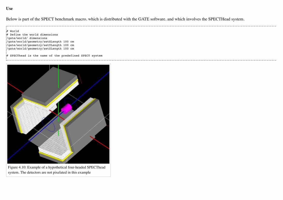
Use

Below is part of the SPECT benchmark macro, which is distributed with the GATE software, and which involves the SPECTHead system.

# World# Define the world dimensions/gate/world/ dimensions /gate/world/geometry/setXLength 100 cm /gate/world/geometry/setYLength 100 cm /gate/world/geometry/setZLength 100 cm

# SPECThead is the name of the predefined SPECT system

Figure 4.10: Example of a hypothetical four-headed SPECTheadsystem. The detectors are not pixelated in this example

# Create the SPECT system, which will yield # an Interfile output of the projection data /gate/world/daughters/name /gate/SPECThead /gate/world/daughters/insert box

# Define the dimensions /gate/SPECThead/geometry/setXLength 7. cm /gate/SPECThead/geometry/setYLength 21. cm /gate/SPECThead/geometry/setZLength 30. cm

# Define the position /gate/SPECThead/placement/setTranslation 20.0 0. 0. cm

# Set the material associated with the main volume /gate/SPECThead/setMaterial Air

# Replicate the head (around the Z axis by default)# to get a hypothetical four-headed system /gate/SPECThead/repeaters/insert ring /gate/SPECThead/ring/setRepeatNumber 4 /gate/SPECThead/ring/setAngularPitch 90. deg

# Define the rotation speed of the head # Define the orbiting around the Z axis /gate/SPECThead/moves/insert orbiting /gate/SPECThead/orbiting/setSpeed 0.15 deg/s /gate/SPECThead/orbiting/setPoint1 0 0 0 cm /gate/SPECThead/orbiting/setPoint2 0 0 1 cm

# Define visualisation options /gate/SPECThead/vis/forceWireframe

# Collimator# Create a full volume defining the shape of# the collimator (typical for SPECT) /gate/SPECThead/daughters/name /gate/collimator /gate/SPECThead/daughters/insert box

# Define the dimensions of the collimator volume /gate/collimator/geometry/setXLength 3. cm /gate/collimator/geometry/setYLength 19. cm /gate/collimator/geometry/setZLength 28. cm

# Define the position of the collimator volume /gate/collimator/placement/setTranslation -2. 0. 0. cm

# Set the material of the collimator volume /gate/collimator/setMaterial Lead

# Define some visualisation options

/gate/collimator/vis/setColor red /gate/collimator/vis/forceWireframe

# Insert the first hole of air in the collimator /gate/collimator/daughters/name /gate/hole /gate/collimator/daughters/insert hexagone /gate/hole/geometry/setHeight 3. cm /gate/hole/geometry/setRadius .15 cm /gate/hole/placement/setRotationAxis 0 1 0 /gate/hole/placement/setRotationAngle 90 deg /gate/hole/setMaterial Air # Repeat the hole in an array /gate/hole/repeaters/insert cubicArray /gate/hole/cubicArray/setRepeatNumberX 1 /gate/hole/cubicArray/setRepeatNumberY 52 /gate/hole/cubicArray/setRepeatNumberZ 44 /gate/hole/cubicArray/setRepeatVector 0. 0.36 0.624 cm # Repeat linearly these holes /gate/hole/repeaters/insert linear /gate/hole/linear/setRepeatNumber 2 /gate/hole/linear/setRepeatVector 0. 0.18 0.312 cm /gate/hole/attachPhantomSD

# Crystal # Create the crystal volume /gate/SPECThead/daughters/name crystal /gate/SPECThead/daughters/insert box

# Define the dimensions of the crystal volume /gate/crystal/geometry/setXLength 1. cm /gate/crystal/geometry/setYLength 19. cm /gate/crystal/geometry/setZLength 28. cm

# Define the position of the crystal volume /gate/crystal/placement/setTranslation 0. 0. 0. cm

# Set the material associated with the crystal volume /gate/crystal/setMaterial NaI /gate/crystal/attachCrystalSD

# The SPECThead system is made of three levels: base (for the head), #crystal (for the crystal and crystal matrix) and pixel #(for individual crystals for pixelated gamma camera) /gate/systems/SPECThead/crystal/attach crystal

# Look at the system /gate/systems/SPECThead/describe

Modelling the collimator

SPECT systems need collimator. A parameterized collimator setup was developed for both parallel hole collimators and fan beam collimators. It is based onthe GEANT4 replica system in which a single volume represents multiple copies of a volume (the air holes) within its mother volume (the collimator itself).SPECT collimator geometries are built using this approach in less than a second.

Example for parallel hole collimators:

/gate/SPECThead/daughters/name colli #specify that the parallel beam collimator setup must be used/gate/SPECThead/daughters/insert parallelbeam #set the collimator material/gate/colli/setMaterialName Lead #set the collimator dimensions/gate/colli/geometry/setDimensionX 70 cm/gate/colli/geometry/setDimensionY 80 cm #set the thickness of the collimator/gate/colli/geometry/setHeight 3 cm #specify the hole radius/gate/colli/geometry/setInnerRadius 0.5 cm #set the septal thickness to the required distance between the holes/gate/colli/geometry/setSeptalThickness 0.2 cm /gate/colli/placement/alignToX/gate/colli/placement/setRotationAxis 0 0 1/gate/colli/placement/setRotationAngle -90 deg

/!\_/!\_/!\_/!\ Fan Beam option is out of order - Should be debug ASAP /!\_/!\_/!\_/!\

Example of code for modelling fanbeam collimators:

/gate/SPECThead/daughters/name fanbeam/gate/SPECThead/daughters/insert collimator #set the material for the collimator/gate/fanbeam/setMaterial Lead #define the X and Y size of the collimator/gate/fanbeam/geometry/setDimensionY 53.5 cm

/gate/fanbeam/geometry/setDimensionX 25.0 cm #specify the focal length/gate/fanbeam/geometry/setFocalDistanceY 0.0 cm/gate/fanbeam/geometry/setFocalDistanceX 35.0 cm #specify the thickness of the collimator/gate/fanbeam/geometry/setHeight 5.8 cm #set the septal thickness to the required distance between the holes/gate/fanbeam/geometry/setSeptalThickness 0.8 cm #specify the hole radius/gate/fanbeam/geometry/setInnerRadius 1.70 cm/gate/fanbeam/placement/setRotationAxis 0 0 1 /gate/fanbeam/placement/setRotationAngle -90 deg /gate/fanbeam/vis/setColor blue/gate/fanbeam/vis/forceWireframe

Septal Penetration

If one wants to record, for every photon detected, how many times they crossed the collimator septa, the command recordSeptalPenetration must be turnedon (default value is false) and the septal volume name must be attached to a PhantomSD:

/gate/output/analysis/recordSeptalPenetration true/gate/output/analysis/setSeptalVolumeName collimator

If the septal volume name does not exist, the simulation is aborted.

OpticalSystem

Description

OpticalSystem is appropriate to model Optical Imaging within GATE. An example macro defining a typical Optical Imaging system can be found in:

https://github.com/OpenGATE/GateContrib/blob/master/imaging/Optical/Optical_System.mac

An OpticalSystem is a box-shaped geometry element and consists of three hierarchic levels:

Figure 4.11: Example of ahypothetical OpticalImagingpixelated system. A pixelated camerais simulated in red. The additionalvolume in yellow could representsome electronic board.

base which is always attached to the volume OpticalSystem.crystal which is coupled to the main detector block.pixel which can be used for modeling a pixelated detector.

Use

Below is part of the Optical Imaging benchmark macro, which is distributed with the GATE software.

# World# Define the world dimensions/gate/world/geometry/setXLength 100. cm/gate/world/geometry/setYLength 100. cm/gate/world/geometry/setZLength 100. cm/gate/world/setMaterial Air

# Create the Optical Imaging system, which will yield # a binary output of the projection data /gate/world/daughters/name OpticalSystem/gate/world/daughters/insert box

# Define the dimensions, position and material /gate/OpticalSystem/geometry/setXLength 10.5 cm/gate/OpticalSystem/geometry/setYLength 10.5 cm/gate/OpticalSystem/geometry/setZLength 2.0 cm/gate/OpticalSystem/placement/setTranslation 0 0 0 cm/gate/OpticalSystem/setMaterial Air

# Define pixelated detector: /gate/OpticalSystem/daughters/name crystal/gate/OpticalSystem/daughters/insert box/gate/crystal/geometry/setXLength 10.5 cm/gate/crystal/geometry/setYLength 10.5 cm/gate/crystal/geometry/setZLength 1.0 cm/gate/crystal/placement/setTranslation 0 0 -0.5 cm/gate/crystal/setMaterial Air/gate/crystal/vis/forceWireframe 1/gate/systems/OpticalSystem/crystal/attach crystal

/gate/crystal/daughters/name pixel/gate/crystal/daughters/insert box/gate/pixel/geometry/setXLength 2.0 cm/gate/pixel/geometry/setYLength 2.0 cm/gate/pixel/geometry/setZLength 1.0 cm/gate/pixel/setMaterial Air/gate/pixel/placement/setTranslation 0 0 0 cm/gate/pixel/vis/setColor red/gate/pixel/repeaters/insert cubicArray

/gate/pixel/cubicArray/setRepeatNumberX 5/gate/pixel/cubicArray/setRepeatNumberY 5/gate/pixel/cubicArray/setRepeatNumberZ 1/gate/pixel/cubicArray/setRepeatVector 2.1 2.1 0 cm/gate/pixel/vis/forceSolid /gate/pixel/attachCrystalSD/gate/systems/OpticalSystem/pixel/attach pixel

# Define an additional volume behind the pixels/gate/OpticalSystem/daughters/name Electronics/gate/OpticalSystem/daughters/insert box/gate/Electronics/geometry/setXLength 10.5 cm/gate/Electronics/geometry/setYLength 10.5 cm/gate/Electronics/geometry/setZLength 1.0 cm/gate/Electronics/setMaterial Air /gate/Electronics/placement/setTranslation 0 0 0.5 cm/gate/Electronics/vis/setColor yellow/gate/Electronics/vis/forceSolid

How to define a multi-system detectorTo simulate a multi-system device consisting of several detectors (PET,SPECT,CT,..) you need to add in your macro special commands as explained below.This will allow you to simultaneously register Hits inside every detector.

Defining the systems:

The standard definition of a GATE system is done according to the command:

/gate/world/daughters/name SystemName

Where SystemName must be one of available system names in GATE (see table 4.1). Unfortunately, defining a system with this command prevent you toinsert more than one system of the same type. Another method has been inserted in GATE to define more than one system at a time. Using this more generalmethod, users can simulate several systems simultaneously. A system is now defined by its own name and its type according to the next two command lines:

/gate/world/daughters/name AnyName/gate/world/daughters/systemType SystemType

Where AnyName can be any name as for any Geant4 volume name and SystemType must be one the names of GATE systems mentioned in table 4.1.

How to connect the geometry to the systems:

By using more than one system, we have to change the attachment commands to connect the geometrical elements of every system with its definedcomponents, to do that we use the next command:

/gate/systems/SystemName/Level/attach UserVolumeName

This command has the same form as for one system, but the essential difference is that SystemName here can be any name gave by the user to the system.

Example of multi-system:

An example for the creation of three systems, one system of type “cylindricalPET” and two systems of type “scanner” is explained below. Note that it is notnecessary to use the “ systemType” command for cylindricalPET system because there is only one system of this type.

# W O R L D /gate/world/geometry/setXLength 40. cm /gate/world/geometry/setYLength 40. cm /gate/world/geometry/setZLength 60. cm

# M O U S E /gate/world/daughters/name mouse /gate/world/daughters/insert cylinder /gate/mouse/setMaterial Water /gate/mouse/vis/setColor red /gate/mouse/geometry/setRmax 18.5 mm /gate/mouse/geometry/setRmin 0. mm /gate/mouse/geometry/setHeight 68. mm

# SYSTEM 1: cylindricalPET /gate/world/daughters/name cylindricalPET # standard definition/gate/world/daughters/insert cylinder /gate/cylindricalPET/setMaterial Water /gate/cylindricalPET/geometry/setRmax 145 mm /gate/cylindricalPET/geometry/setRmin 130 mm /gate/cylindricalPET/geometry/setHeight 80 mm /gate/cylindricalPET/vis/forceWireframe

#cylindricalPET => rsector /gate/cylindricalPET/daughters/name rsector /gate/cylindricalPET/daughters/insert box /gate/rsector/placement/setTranslation 135 0 0 mm /gate/rsector/geometry/setXLength 10. mm

/gate/rsector/geometry/setYLength 19. mm /gate/rsector/geometry/setZLength 76.6 mm /gate/rsector/setMaterial Water /gate/rsector/vis/forceWireframe

#cylindricalPET => module /gate/rsector/daughters/name module /gate/rsector/daughters/insert box /gate/module/geometry/setXLength 10. mm /gate/module/geometry/setYLength 19. mm /gate/module/geometry/setZLength 19. mm /gate/module/setMaterial Water /gate/module/vis/forceWireframe /gate/module/vis/setColor gray

#cylindricalPET => crystal /gate/module/daughters/name crystal /gate/module/daughters/insert box /gate/crystal/geometry/setXLength 10. mm /gate/crystal/geometry/setYLength 2.2 mm /gate/crystal/geometry/setZLength 2.2 mm /gate/crystal/setMaterial Water /gate/crystal/vis/forceWireframe /gate/crystal/vis/setColor magenta

#cylindricalPET => LSO /gate/crystal/daughters/name LSO /gate/crystal/daughters/insert box /gate/LSO/geometry/setXLength 10. mm /gate/LSO/geometry/setYLength 2.2 mm /gate/LSO/geometry/setZLength 2.2 mm /gate/LSO/placement/setTranslation 0 0 0 mm /gate/LSO/setMaterial LSO /gate/LSO/vis/setColor yellow

# R E P E A T C R Y S T A L /gate/crystal/repeaters/insert cubicArray /gate/crystal/cubicArray/setRepeatNumberX 1 /gate/crystal/cubicArray/setRepeatNumberY 8 /gate/crystal/cubicArray/setRepeatNumberZ 8 /gate/crystal/cubicArray/setRepeatVector 10. 2.4 2.4 mm

# R E P E A T M O D U L E /gate/module/repeaters/insert cubicArray /gate/module/cubicArray/setRepeatNumberZ 4 /gate/module/cubicArray/setRepeatVector 0. 0. 19.2 mm

# R E P E A T R S E C T O R /gate/rsector/repeaters/insert ring /gate/rsector/ring/setRepeatNumber 42

# SYSTEM 2: Scanner_1 /gate/world/daughters/name Scanner_1 # System name definition for scanner 1/gate/world/daughters/systemType scanner # System type definition for scanner 1/gate/world/daughters/insert box /gate/Scanner_1/setMaterial Air /gate/Scanner_1/geometry/setXLength 20 cm /gate/Scanner_1/geometry/setYLength 20 cm /gate/Scanner_1/geometry/setZLength 10 cm /gate/Scanner_1/placement/setTranslation 0 0 -18 cm /gate/Scanner_1/vis/forceWireframe /gate/Scanner_1/vis/setVisible 1

# Scanner_1 => Cryostat_1 /gate/Scanner_1/daughters/name Cryostat_1 /gate/Scanner_1/daughters/insert box /gate/Cryostat_1/placement/setTranslation 0 0 0 cm /gate/Cryostat_1/geometry/setXLength 19 cm /gate/Cryostat_1/geometry/setYLength 19 cm /gate/Cryostat_1/geometry/setZLength 9 cm /gate/Cryostat_1/setMaterial Stainless /gate/Cryostat_1/vis/setColor yellow /gate/Cryostat_1/vis/forceWireframe

# Scanner_1 => ActiveZone_1 /gate/Cryostat_1/daughters/name ActiveZone_1 /gate/Cryostat_1/daughters/insert box /gate/ActiveZone_1/placement/setTranslation 0 0 0 cm /gate/ActiveZone_1/geometry/setXLength 18 cm /gate/ActiveZone_1/geometry/setYLength 18 cm /gate/ActiveZone_1/geometry/setZLength 8 cm /gate/ActiveZone_1/setMaterial LXenon /gate/ActiveZone_1/vis/setColor white

# SYSTEM 3: Scanner_2 /gate/world/daughters/name Scanner_2 # System name definition for scanner 2/gate/world/daughters/systemType scanner # System Type definition for scanner 2

/gate/world/daughters/insert box /gate/Scanner_2/setMaterial Air /gate/Scanner_2/geometry/setXLength 20 cm /gate/Scanner_2/geometry/setYLength 20 cm /gate/Scanner_2/geometry/setZLength 10 cm /gate/Scanner_2/placement/setTranslation 0 0 18 cm /gate/Scanner_2/vis/forceWireframe /gate/Scanner_2/vis/setVisible 1

# Scanner_2 => Cryostat_2 /gate/Scanner_2/daughters/name Cryostat_2 /gate/Scanner_2/daughters/insert box

/gate/Cryostat_2/placement/setTranslation 0 0 0 cm /gate/Cryostat_2/geometry/setXLength 19 cm /gate/Cryostat_2/geometry/setYLength 19 cm /gate/Cryostat_2/geometry/setZLength 9 cm /gate/Cryostat_2/setMaterial Stainless /gate/Cryostat_2/vis/setColor yellow /gate/Cryostat_2/vis/forceWireframe

# Scanner_2 => ActiveZone_2 /gate/Cryostat_2/daughters/name ActiveZone_2 /gate/Cryostat_2/daughters/insert box /gate/ActiveZone_2/placement/setTranslation 0 0 0 cm /gate/ActiveZone_2/geometry/setXLength 18 cm /gate/ActiveZone_2/geometry/setYLength 18 cm /gate/ActiveZone_2/geometry/setZLength 8 cm /gate/ActiveZone_2/setMaterial LXenon /gate/ActiveZone_2/vis/setColor white

# A T T A C H S Y S T E M S /gate/systems/cylindricalPET/rsector/attach rsector /gate/systems/cylindricalPET/module/attach module /gate/systems/cylindricalPET/crystal/attach crystal /gate/systems/cylindricalPET/layer0/attach LSO

# New attachment commands/gate/systems/Scanner_1/level1/attach Cryostat_1 /gate/systems/Scanner_1/level2/attach ActiveZone_1

/gate/systems/Scanner_2/level1/attach Cryostat_2 /gate/systems/Scanner_2/level2/attach ActiveZone_2

# A T T A C H L A Y E R SD /gate/LSO/attachCrystalSD /gate/mouse/attachPhantomSD

/gate/ActiveZone_1/attachCrystalSD

/gate/ActiveZone_2/attachCrystalSD

Notes:

a) The command “systemType” is optional in case of using only one system, but the system name must be one GATE systems (first column in table 4.1) asfor standard definition

b) Same remark, in the case where all systems have different types.

c) In general, one has to use the “systemType” command only for simulating more than one system of the same type.

Retrieved from "http://wiki.opengatecollaboration.org/index.php?title=Users_Guide_V8.0:Defining_a_system&oldid=1033"


Users Guide V8.0:Attaching the sensitive detectorsFrom Wiki OpenGATE

General purposeOnce a model has been defined for the scanner through the construction of a system (see Users Guide V8.0:Defining a system), the next step is to attach asensitive detector (SD) to some volumes of the geometry. As in any Geant4 simulation, these sensitive detectors are used to store information regardinginteractions of a particle in the matter (hits) using information from the steps occuring along the particle track. A hit is a snapshot of a physical interaction ofa track in a sensitive region of the detector. Figure 5.1 illustrates these notions. Hits contain various pieces of information associated to a step object, such asthe energy deposition of a step, geometrical information, position and time of a step, etc.

Figure 5.1: Particle interactions in a sensitive detector

GATE records and stores information related to the hits only for those volumes that are attached to a sensitive detector. All information regarding theinteractions occuring in non-sensitive volumes is lost.

The crystalSD

The crystalSD is used to record information regarding interactions taking place inside the volumes belonging to a scanner for instance (crystals orcollimators) : energy deposition, positions of interaction, origin of the particle (emission vertex), type of interaction (name of the physical processesinvolved), etc.

A crystalSD can be attached only to those volumes that belong to a given system. Once a crystalSD has been attached, it is considered as attached to thissystem. This sensitive detector can be attached using the command attachCrystalSD. These volumes are essentially meant to be scintillating elements(crystals) but can also be attached to non-scintillating elements such as collimators, shields or septa.

Below is an example of command lines that should be included in a macro using the crystalSD. These command lines must be inserted after the descriptionof the attachment to the system:

The first command is used to attach the scintillation crystal to the detection levelcrystal of the SPECThead system.

/systems/SPECThead/crystal/attach crystal

Then, the second command attaches the crystalSD to the volume representing the scintillation crystal in the geometry.


The phantomSD

The phantomSD plays a crucial role in GATE simulations, as it is used to record information regarding Compton and Rayleigh interactions taking place inthe volumes before the detection in the scanner system (e.g., for a SPECT camera, these volumes can be the table, phantom, and collimator, in which it canbe relevant to retrieve information about Compton and Rayleigh interactions). These data can then be used to estimate whether a photon reaching a detectoris a direct or a Compton-scattered photon. Thus, in PET, the phantomSD is currently the only way to discriminate scattered from true coincidences. Tosimulate low energy X-ray acquisitions (for example mammography acquisitions from 7 to 28 keV), information concerning Rayleigh interactions issignificant.

Using this type of sensitive detector, it is possible to retrieve two pieces of information related to the hits:

The number of Compton and Rayleigh interactions occuring in all the volumes attached to the phantomSD : nPhantomCompton andnPhantomRayleigh. These pieces of information are also available for the crystalSD with the variables nCrystalCompton and nCrystalRayleigh. Itis impossible to attach both sensitive detectors to the same volume.The last volume attached to the phantomSD in which a Compton or a Rayleigh interaction occured : compVolName and RayleighVolName.

IMPORTANT: To retrieve data output information regarding hits occuring in the phantomSD (nPhantomCompton and compVolName), a crystalSD has tobe defined in the simulation. Otherwise, data output variables will be created but will be empty. When all these conditions are satisfied, any interactiontaking place within the field of view (FOV) of the scanner is automatically recorded by the phantomSD, so that the number of Compton interactions for eachphoton can be accurately computed.

This procedure does not take into account Compton interactions taking place within the detectors, so that inter-crystal cross-talk via Compton interactions isnot detected. Here is an example of command-lines that should be included within the macro in order to use the phantomSD. These command lines must beinserted after the description of the attachment to the system. First, commands are used to attach the scattering volumes to the detection level base of theSPECThead system:

/systems/SPECThead/base/attach FOV /systems/SPECThead/base/attach head /systems/SPECThead/base/attach body

Then, we can attach the phantomSD to the volumes representing the scattering volumes in the geometry :

/FOV/attachPhantomSD /head/attachPhantomSD /body/attachPhantomSD

Finally, the last commands are used to attach the scintillation crystal to the detection level crystal of the SPECThead system and to attach the crystalSD tothe volume representing the scintillation crystal in the geometry.

/systems/SPECThead/crystal/attachCrystalSD /gate/crystal/attachCrystalSD

In the case of a voxellized matrix: Previous commands to attach sensitive detectors are used for the volumes created using the geometry commands ofGATE (see Users Guide V7.2:Defining a geometry). In order to record the same information concerning the interactions occuring in a voxellized matrix, seeUsers Guide V7.2:Voxelized_Source_and_Phantom.

Retrieved from "http://wiki.opengatecollaboration.org/index.php?title=Users_Guide_V8.0:Attaching_the_sensitive_detectors&oldid=556"

This page was last modified on 7 September 2016, at 09:31.

Users Guide V8.0:Digitizer and readout parametersFrom Wiki OpenGATE

Contents1 General Purpose

1.1 From particle detection to coincidences in GATE1.1.1 Definition of a hit in Geant4

1.2 Role of the digitizer1.3 Disabling the digitizer

2 Digitizer modules2.1 Distributions2.2 Adder2.3 Adder Compton2.4 Readout2.5 Blurring : Energy blurring2.6 Blurring : crystal blurring2.7 Blurring : Local energy blurring for different crystals2.8 Blurring: Intrinsic resolution blurring with crystals of different compositions2.9 Calibration2.10 Crosstalk2.11 Thresholder & Upholder2.12 Energy windows2.13 Sigmoidal thresholder2.14 Time resolution2.15 Spatial blurring2.16 Noise2.17 Local efficiency2.18 Memory buffers and bandwidth2.19 Pile-up2.20 Dead time

3 Multiple processor chains

4 Coincidence sorter4.1 Delayed coincidences4.2 Multiple coincidences4.3 Command line

5 Multiple coincidence sorters6 Coincidence processing and filtering

6.1 Coincidence pulse processors6.2 Coincidence dead time6.3 Coincidence buffers6.4 Multiple coincidence removal

7 Example of a digitizer setting8 Digitizer optimization9 Angular Response Functions to speed-up planar or SPECT simulations

9.1 Calculation of the data needed to derive the ARF tables9.2 Computation of the ARF tables from the simulated data9.3 Use of the ARF tables

10 Multi-system approaches: how to use more than one system in one simuation set-up ?10.1 SystemFilter10.2 How to manage the coincidence sorter with more than one system: the Tri Coincidence Sorter approach

General PurposeThe purpose of the digitizer module is to simulate the behaviour of the scanner detectors and signal processing chain.

From particle detection to coincidences in GATE

GATE uses Geant4 to generate particles and transport them through the materials. This mimics physical interactions between particles and matter. Theinformation generated during this process is used by GATE to simulate the detector pulses (digits), which correspond to the observed data. The digitizerrepresents the series of steps and filters that make up this process.

The typical data-flow for an event is as follows:

A particle is generated, with its parameters, such as initial type, time, momentum, and energy.An elementary trajectory step is applied. A step corresponds to the trajectory of a particle between discrete interactions (i.e. photoelectric, Compton,

pair production, etc). During a step, the changes to particle's energy and momentum are calculated. The length of a step depends upon the nature of theinteraction, the type of particle and material, etc. The calculation of the step length is complex and is mentioned here only briefly. For more details,please refer to the Geant4 documentation.If a step occurs within a volume corresponding to a sensitive detector, the interaction information between the particle and the material is stored. Forexample, this information may include the deposited energy, the momentum before and after the interaction, the name of the volume where theinteraction occurred, etc. This set of information is referred to as a Hit.Steps 2 and 3 are repeated until the energy of the particle becomes lower than a predefined value, or the particle position goes outside the predefinedlimits. The entire series of steps form a simulated trajectory of a particle, that is called a Track in Geant4.The amount of energy deposited in a crystal is filtered by the digitizer module. The output from the digitizer corresponds to the signal after it has beenprocessed by the Front End Electronics (FEE). Generally, the FEE is made of several processing units, working in a serial and/or in parallel. Thisprocess of transforming the energy of a Hit into the final digital value is called Digitization and is performed by the GATE digitizer. Each processingunit in the FEE is represented in GATE by a corresponding digitizer module. The final value obtained after filtering by a set of these modules is calleda Single. Singles can be saved as output. Each transient value, between two modules, is called a Pulse.

This process is repeated for each event in the simulation in order to produce one or more sets of Singles. These Singles can be stored into an output file (as aROOT tree, for example).

In case of PET systems, a second processing stage can be inserted to sort the Singles list for coincidences. To do this, the algorithm searches in this list for aset of Singles that are detected within a given time interval (the so called 'coincident events').

Finally, the coincidence data may be filtered-out to mimic any possible data loss which could occur in the coincidence logical circuit or during the datatransportation. As for the Singles, the processing is performed by specifying a list of generic modules to apply to the coincidence data flow.

Definition of a hit in Geant4

A hit is a snapshot of the physical interaction of a track within a sensitive region of a detector. The information given by a hit is

Position and time of the stepMomentum and energy of the trackEnergy deposition of the stepInteraction type of the hitVolume name containing the hit

As a result, the history of a particle is saved as a series of hits generated along the particles trajectory. In addition to the physical hits, Geant4 saves a specialhit. This hit takes place when a particle moves from one volume to another (this type of hit deposits zero energy). The hit data represents the basicinformation that a user has with which to construct the physically observable behaviour of a scanner. To see the information stored in a hit, see the file

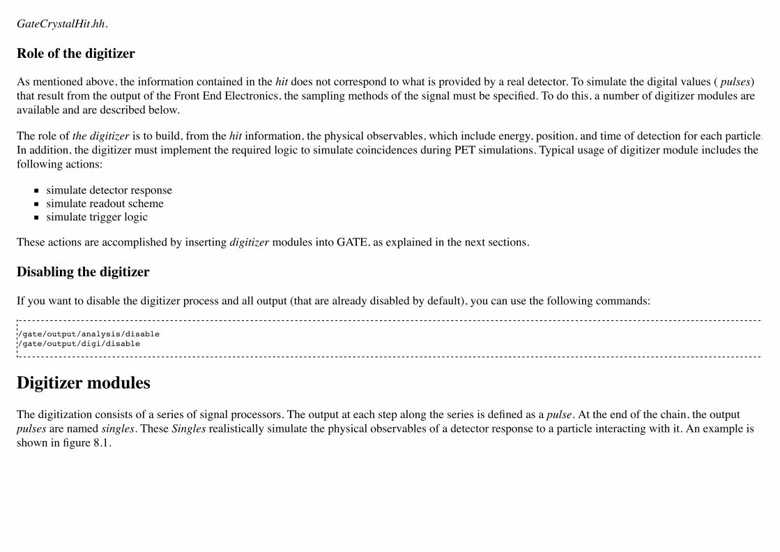
GateCrystalHit.hh.

Role of the digitizer

As mentioned above, the information contained in the hit does not correspond to what is provided by a real detector. To simulate the digital values ( pulses)that result from the output of the Front End Electronics, the sampling methods of the signal must be specified. To do this, a number of digitizer modules areavailable and are described below.

The role of the digitizer is to build, from the hit information, the physical observables, which include energy, position, and time of detection for each particle.In addition, the digitizer must implement the required logic to simulate coincidences during PET simulations. Typical usage of digitizer module includes thefollowing actions:

simulate detector responsesimulate readout schemesimulate trigger logic

These actions are accomplished by inserting digitizer modules into GATE, as explained in the next sections.

Disabling the digitizer

If you want to disable the digitizer process and all output (that are already disabled by default), you can use the following commands:

/gate/output/analysis/disable/gate/output/digi/disable

Digitizer modulesThe digitization consists of a series of signal processors. The output at each step along the series is defined as a pulse. At the end of the chain, the outputpulses are named singles. These Singles realistically simulate the physical observables of a detector response to a particle interacting with it. An example isshown in figure 8.1.

Figure 8.1: The digitizer is organized as a chain of modules that begins with the hit and ends with the single which represents the physicalobservable seen from the detector.

To specify a new signal-processing module (i.e. add a new processing unit in the readout scheme) the following command template should be used :

/gate/digitizer/insert MODULE

where MODULE is the name of the digitizer module. The order of the module declaration should make sense. The data flow follows the same order as themodule declaration in the macro. In a typical scanner, the following sequence works well, athough it is not mandatory (the module names will be explainedin the rest of the section):

insert adder before readoutinsert readout before thresholder/upholderinsert blurring before thresholder/upholder

Distributions

Since many of the modules presented below have to deal with functions or probability density, a generic tool is provided to describe such mathematicalobjects in GATE. Basically, a distribution in GATE is defined by its name, its type (Gaussian, Exponential, etc...) and the parameters specifics to eachdistribution type (such as the mean and the standard deviation of a Gaussian function). Depending on the context, these objects are used directly asfunctions, or as probability densities into which a variable is randomly chosen. In the following, the generic term of distribution will be used to describe bothof these objects, since their declaration is unified under this term into GATE.

Five types of distribution are available in GATE, namely:

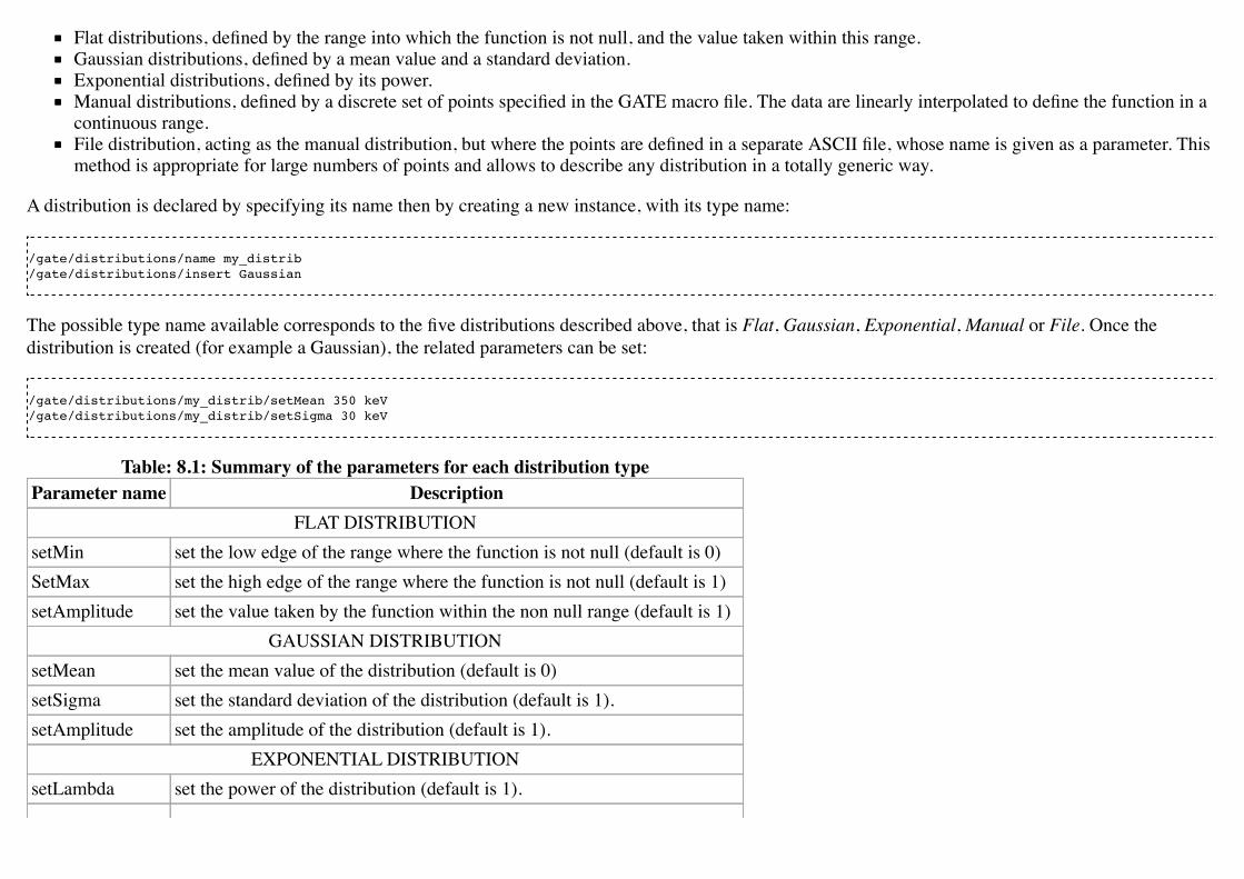
Flat distributions, defined by the range into which the function is not null, and the value taken within this range.Gaussian distributions, defined by a mean value and a standard deviation.Exponential distributions, defined by its power.Manual distributions, defined by a discrete set of points specified in the GATE macro file. The data are linearly interpolated to define the function in acontinuous range.File distribution, acting as the manual distribution, but where the points are defined in a separate ASCII file, whose name is given as a parameter. Thismethod is appropriate for large numbers of points and allows to describe any distribution in a totally generic way.

A distribution is declared by specifying its name then by creating a new instance, with its type name:

/gate/distributions/name my_distrib /gate/distributions/insert Gaussian

The possible type name available corresponds to the five distributions described above, that is Flat, Gaussian, Exponential, Manual or File. Once thedistribution is created (for example a Gaussian), the related parameters can be set:

/gate/distributions/my_distrib/setMean 350 keV /gate/distributions/my_distrib/setSigma 30 keV

Table: 8.1: Summary of the parameters for each distribution typeParameter name Description

FLAT DISTRIBUTIONsetMin set the low edge of the range where the function is not null (default is 0)SetMax set the high edge of the range where the function is not null (default is 1)setAmplitude set the value taken by the function within the non null range (default is 1)

GAUSSIAN DISTRIBUTIONsetMean set the mean value of the distribution (default is 0)setSigma set the standard deviation of the distribution (default is 1).setAmplitude set the amplitude of the distribution (default is 1).

EXPONENTIAL DISTRIBUTIONsetLambda set the power of the distribution (default is 1).

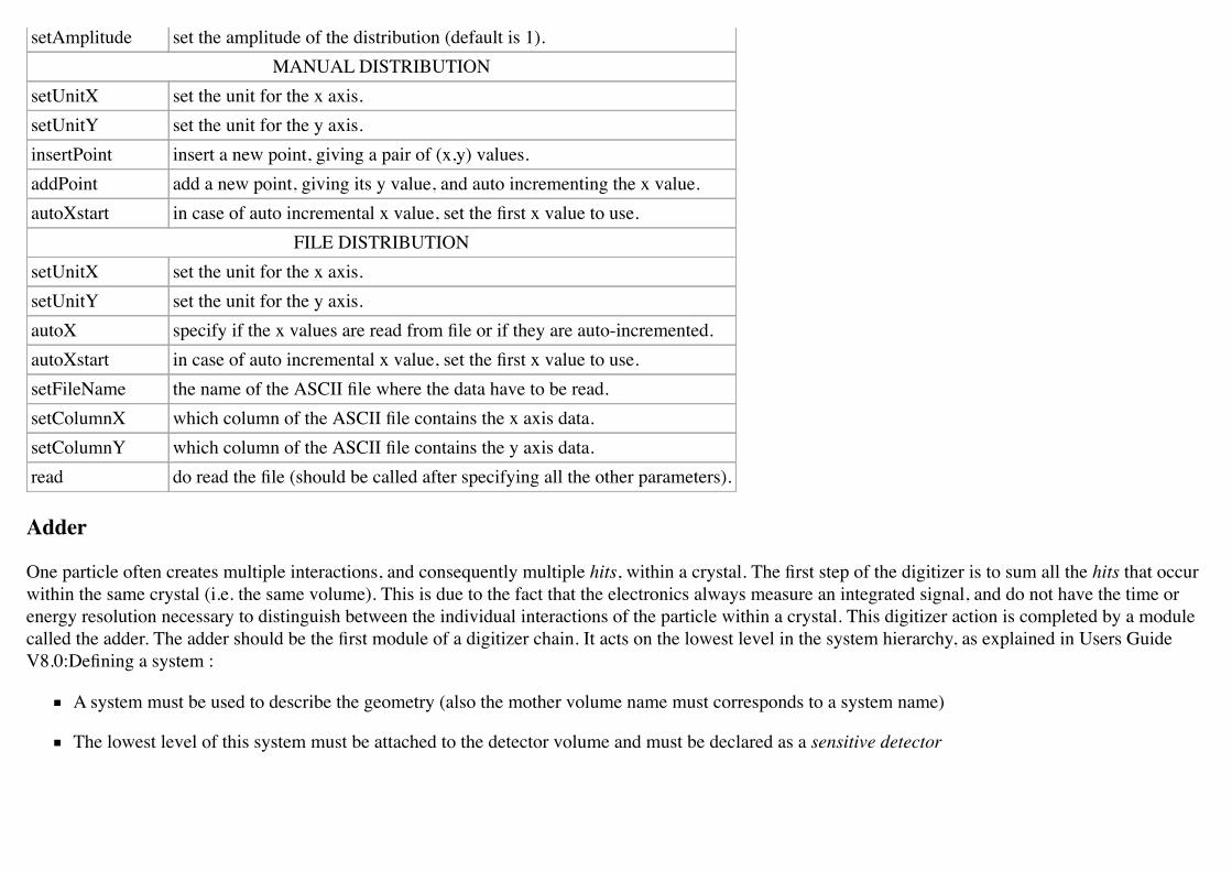
setAmplitude set the amplitude of the distribution (default is 1).MANUAL DISTRIBUTION

setUnitX set the unit for the x axis.setUnitY set the unit for the y axis.insertPoint insert a new point, giving a pair of (x,y) values.addPoint add a new point, giving its y value, and auto incrementing the x value.autoXstart in case of auto incremental x value, set the first x value to use.

FILE DISTRIBUTIONsetUnitX set the unit for the x axis.setUnitY set the unit for the y axis.autoX specify if the x values are read from file or if they are auto-incremented.autoXstart in case of auto incremental x value, set the first x value to use.setFileName the name of the ASCII file where the data have to be read.setColumnX which column of the ASCII file contains the x axis data.setColumnY which column of the ASCII file contains the y axis data.read do read the file (should be called after specifying all the other parameters).

Adder

One particle often creates multiple interactions, and consequently multiple hits, within a crystal. The first step of the digitizer is to sum all the hits that occurwithin the same crystal (i.e. the same volume). This is due to the fact that the electronics always measure an integrated signal, and do not have the time orenergy resolution necessary to distinguish between the individual interactions of the particle within a crystal. This digitizer action is completed by a modulecalled the adder. The adder should be the first module of a digitizer chain. It acts on the lowest level in the system hierarchy, as explained in Users GuideV8.0:Defining a system :

A system must be used to describe the geometry (also the mother volume name must corresponds to a system name)

The lowest level of this system must be attached to the detector volume and must be declared as a sensitive detector

The adder regroups hits per volume into a pulse. If one particle that enters a detector makes multiple hits within two different crystal volumes before beingstopped, the output of the adder module will consists of two pulses. Each pulse is computed as follows : the energy is taken to be the total of energies in eachvolume, the position is obtained with an energy-weighted centroid of the different hit positions. The time is equal to the time at which the first hit occured.

The command to use the adder module is

/gate/digitizer/Singles/insert adder

Adder Compton

The adderCompton module has a different behavior than the classic adder, which performs an energy-weighted centroid addition of all electronic andphotonic hits. Instead, for each electronic energy deposition, the energy is added to the previous photonic hit in the same volume ID (or discarded if none),but the localization remains that of the photonic interaction. That way, the Compton kinematics becomes exact for photonic interations, enabling furtherstudies. The user must use the classic adder afterwards, to handle multiple photonic interactions in the same crystal. The commands to use the adder moduleare

/gate/digitizer/Singles/insert adderCompton/gate/digitizer/Singles/insert adder

Readout

With the exception of a detector system where each crystal is read by an individual photo-detector, the readout segmentation is often different from the basicgeometrical structures of the detector. The readout geometry is an artificial geometry that is usually associated with a group of sensitive detectors. There aretwo ways of modelling this readout process : either a winner-takes-all approach that will somewhat model APD-like readout, or a energy-centroid approachthat will be closer to the block-PMT readout. Using the winner-takes-all policy, the grouping has to be determined by the user through a variable nameddepth corresponding to the component in the volume hierarchy at which pulses are summed together. Using this variable, the pulses are summed if theirvolume ID's are identical to this level of depth. Using the energy-centroid policy, the depth of the grouping is forced to occur at the 'crystal' level whateverthe system used, so the depth variable is ignored. This means that the pulses in a same level just above the crystal level are summed together.

The readout module regroups pulses per block (group of sensitive detectors). For both policy, the resulting pulse in the block has the total energy of allpulses summed together. For the winner-takes-all policy, the position of the pulse is the one with the maximum energy. For the energy-centroid policy, theposition is determined by weighting the crystal indices of each pulse by the deposited energy in order to get the energy centroid position. In this case, only

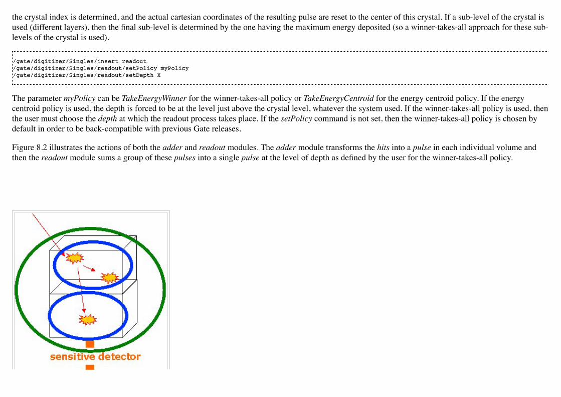
the crystal index is determined, and the actual cartesian coordinates of the resulting pulse are reset to the center of this crystal. If a sub-level of the crystal isused (different layers), then the final sub-level is determined by the one having the maximum energy deposited (so a winner-takes-all approach for these sub-levels of the crystal is used).

/gate/digitizer/Singles/insert readout/gate/digitizer/Singles/readout/setPolicy myPolicy/gate/digitizer/Singles/readout/setDepth X

The parameter myPolicy can be TakeEnergyWinner for the winner-takes-all policy or TakeEnergyCentroid for the energy centroid policy. If the energycentroid policy is used, the depth is forced to be at the level just above the crystal level, whatever the system used. If the winner-takes-all policy is used, thenthe user must choose the depth at which the readout process takes place. If the setPolicy command is not set, then the winner-takes-all policy is chosen bydefault in order to be back-compatible with previous Gate releases.

Figure 8.2 illustrates the actions of both the adder and readout modules. The adder module transforms the hits into a pulse in each individual volume andthen the readout module sums a group of these pulses into a single pulse at the level of depth as defined by the user for the winner-takes-all policy.

Figure 8.2 Actions of the it adder and it readoutmodules

The importance of the setDepth command line when using the winner-takes-all policy is illustrated through the following example from a PET system (seeUsers Guide V8.0:Defining a system). In a cylindricalPET system, where the first volume level is rsector, and the second volume level is module, as shownin figure 8.3, the readout depth depends upon how the electronic readout functions.

If one PMT reads the four modules in the axial direction, the depth should be set with the command:


The energy of this single event is the sum of the energy of the pulses inside the white rectangle (rsector) of figure 8.3. However, if individual PMTs readeach module (group of crystals), the depth should be set with the command:


In this case, the energy of the single event is the sum of the energies of the pulses inside the red box (module) of figure 8.3.

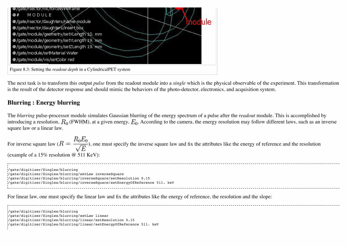
Figure 8.3: Setting the readout depth in a CylindricalPET system

The next task is to transform this output pulse from the readout module into a single which is the physical observable of the experiment. This transformationis the result of the detector response and should mimic the behaviors of the photo-detector, electronics, and acquisition system.

Blurring : Energy blurring

The blurring pulse-processor module simulates Gaussian blurring of the energy spectrum of a pulse after the readout module. This is accomplished byintroducing a resolution, (FWHM), at a given energy, . According to the camera, the energy resolution may follow different laws, such as an inversesquare law or a linear law.

For inverse square law ( ), one must specify the inverse square law and fix the attributes like the energy of reference and the resolution

(example of a 15% resolution @ 511 KeV):

/gate/digitizer/Singles/blurring/gate/digitizer/Singles/blurring/setLaw inverseSquare/gate/digitizer/Singles/blurring/inverseSquare/setResolution 0.15/gate/digitizer/Singles/blurring/inverseSquare/setEnergyOfReference 511. keV

For linear law, one must specify the linear law and fix the attributes like the energy of reference, the resolution and the slope:

/gate/digitizer/Singles/blurring/gate/digitizer/Singles/blurring/setLaw linear/gate/digitizer/Singles/blurring/linear/setResolution 0.15/gate/digitizer/Singles/blurring/linear/setEnergyOfReference 511. keV

/gate/digitizer/Singles/blurring/linear/setSlope -0.055 1/MeV

Blurring : crystal blurring

This type of blurring is used for the scanners where all the detectors are made of the same type of crystal. In this case, it is often useful to assign a differentenergy resolution for each crystal in the detector block, between a minimum and a maximum value. To model the efficiency of the system, a coefficient(between 0 and 1) can also be set.

As an example, a random blurring of all the crystals between 15% and 35% at a reference energy of 511 keV, and with a quantum efficiency of 90% can bemodelled using the following commands:

/gate/digitizer/Singles/insert crystalblurring /gate/digitizer/Singles/crystalblurring/setCrystalResolutionMin 0.15 /gate/digitizer/Singles/crystalblurring/setCrystalResolutionMax 0.35 /gate/digitizer/Singles/crystalblurring/setCrystalQE 0.9 /gate/digitizer/Singles/crystalblurring/setCrystalEnergyOfReference 511.keV

In this example, for each interaction the program randomly chooses a crystal resolution between 0.15 and 0.35. The crystals are not assigned a constantresolution. The crystal quantum efficiency is set using setCrystalQE and represents the probability for the event to be detected by the photo-detector. Thisparameter represents the effect of the transfer efficiency of the crystal and of the quantum efficiency of the photo-detector.

Blurring : Local energy blurring for different crystals

The LocalBlurring module is very similar to the energy blurring module, but different energy resolutions are applied to different volumes. This type ofblurring is useful for detectors with several layers of different scintillation crystals (e.g. depth of interaction measurement with a phoswich module in aCylindricalPET system).

If a detector has a resolution of 15.3% @ 511 KeV for a crystal called crystal1 and has a resolution of 24.7% @ 511 KeV for another crystal (crystal2) in aphoswich configuration, the following commands should be used:

/gate/digitizer/Singles/insert localBlurring /gate/digitizer/Singles/localBlurring/chooseNewVolume crystal1 /gate/digitizer/Singles/localBlurring/crystal1/setResolution 0.153 /gate/digitizer/Singles/localBlurring/crystal1/setEnergyOfReference 511 keV /gate/digitizer/Singles/localBlurring/chooseNewVolume crystal2 /gate/digitizer/Singles/localBlurring/crystal2/setResolution 0.247 /gate/digitizer/Singles/localBlurring/crystal2/setEnergyOfReference 511 keV

BEWARE: crystal1 and crystal2 must be valid Sensitive Detector volume names !!

Blurring: Intrinsic resolution blurring with crystals of different compositions

This blurring pulse-processor simulates a local Gaussian blurring of the energy spectrum (different for different crystals) based on the following model:

where and , and , are the Light Yield, Transfer, and Quantum Efficiency for each crystal.

is the relative variance of the gain of a Photo Multiplier Tube (PMT) or of an Avalanche Photo Diode (APD). It is hard-codded and set to 0.1.

If the intrinsic resolutions, , of the individual crystals are not defined, then they are set to one.

To use this digitizer module properly, several modules must be set first. These digitizer modules are GateLightYield, GateTransferEfficiency, andGateQuantumEfficiency. The light yield pulse-processor simulates the crystal light yield. Each crystal must be given the correct light yield. This moduleconverts the pulse energy into the number of scintillation photons emitted, . The transfer efficiency pulse-processor simulates the transfer efficiencies ofthe light photons in each crystal. This digitizer reduces the "pulse" energy (by reducing the number of scintillation photons) by a transfer efficiencycoefficient which must be a number between 0 and 1. The quantum efficiency pulse-processor simulates the quantum efficiency for each channel of a photo-detector, which can be a Photo Multiplier Tube (PMT) or an Avalanche Photo Diode (APD).

The command lines are illustrated using an example of a phoswich module made of two layers of different crystals. One crystal has a light yield of 27000photons per MeV (LSO crystal), a transfer efficiency of 28%, and an intrinsic resolution of 8.8%. The other crystal has a light yield of 8500 photons perMeV (LuYAP crystal), a transfer efficiency of 24% and an intrinsic resolution of 5.3%

In the case of a cylindricalPET system, the construction of the crystal geometry is truncated for clarity (the truncation is denoted by ...). The digitizercommand lines are:

# LSO layer /gate/crystal/daughters/name LSOlayer ....

# BGO layer /gate/crystal/daughters/name LuYAPlayer ....

# A T T A C H S Y S T E M .... /gate/systems/cylindricalPET/crystal/attach crystal /gate/systems/cylindricalPET/layer0/attach LSOlayer /gate/systems/cylindricalPET/layer1/attach LuYAPlayer

# A T T A C H C R Y S T A L S D /gate/LSOlayer/attachCrystalSD /gate/LuYAPlayer/attachCrystalSD

# In this example the phoswich module is represented by the crystal volume and is made of two different material layers. # To apply the resolution blurring of equation , the parameters discussed above must be defined for each layer #(i.e. Light Yield, Transfer, Intrinsic Resolution, and the Quantum Efficiency).# DEFINE TRANSFER EFFICIENCY FOR EACH LAYER /gate/digitizer/Singles/insert transferEfficiency /gate/digitizer/Singles/transferEfficiency/chooseNewVolume LSOlayer /gate/digitizer/Singles/transferEfficiency/LSOlayer/setTECoef 0.28 /gate/digitizer/Singles/transferEfficiency/chooseNewVolume LuYAPlayer /gate/digitizer/Singles/transferEfficiency/LuYAPlayer/setTECoef 0.24

# DEFINE LIGHT YIELD FOR EACH LAYER /gate/digitizer/Singles/insert lightYield /gate/digitizer/Singles/lightYield/chooseNewVolume LSOlayer /gate/digitizer/Singles/lightYield/LSOlayer/setLightOutput 27000 /gate/digitizer/Singles/lightYield/chooseNewVolume LuYAPlayer /gate/digitizer/Singles/lightYield/LuYAPlayer/setLightOutput 8500

# DEFINE INTRINSIC RESOLUTION FOR EACH LAYER /gate/digitizer/Singles/insert intrinsicResolutionBlurring /gate/digitizer/Singles/intrinsicResolutionBlurring/ chooseNewVolume LSOlayer /gate/digitizer/Singles/intrinsicResolutionBlurring/ LSOlayer/setIntrinsicResolution 0.088 /gate/digitizer/Singles/intrinsicResolutionBlurring/ LSOlayer/setEnergyOfReference 511 keV /gate/digitizer/Singles/intrinsicResolutionBlurring/ chooseNewVolume LuYAPlayer /gate/digitizer/Singles/intrinsicResolutionBlurring/ LuYAPlayer/setIntrinsicResolution 0.053 /gate/digitizer/Singles/intrinsicResolutionBlurring/ LuYAPlayer/setEnergyOfReference 511 keV

# DEFINE QUANTUM EFFICIENCY OF THE PHOTODETECTOR /gate/digitizer/Singles/insert quantumEfficiency /gate/digitizer/Singles/quantumEfficiency/chooseQEVolume crystal /gate/digitizer/Singles/quantumEfficiency/setUniqueQE 0.1

Note: A complete example of a phoswich module can be in the PET benchmark.

Note for Quantum Efficiency

With the previous commands, the same quantum efficiency will be applied to all the detector channels. The user can also provide lookup tables for eachdetector module. These lookup tables are built from the user files.

To set multiple quantum efficiencies using files (fileName1, fileName2, ... for each of the different modules), the following commands can be used:

/gate/digitizer/Singles/insert quantumEfficiency /gate/digitizer/Singles/quantumEfficiency/chooseQEVolume crystal /gate/digitizer/Singles/quantumEfficiency/useFileDataForQE fileName1 /gate/digitizer/Singles/quantumEfficiency/useFileDataForQE fileName2

If the crystal volume is a daughter of a module volume which is an array of 8 x 8 crystals, the file fileName1 will contain 64 values of quantum efficiency. Ifseveral files are given (in this example two files), the program will choose randomly between theses files for each module.

Important note

After the introduction of the lightYield (LY), transferEfficiency and quantumEfficiency} modules, the energy variable of a pulse is not in energy unit(MeV) but in number of photoelectrons .

In order to correctly apply a threshold on a phoswhich module, the threshold should be based on this number and not on the real energy. In this situation, toapply a threshold at this step of the digitizer chain, the threshold should be applied as explained in #Thresholder & Upholder. In this case, the GATEprogram knows that these modules have been used, and will apply threshold based upon the number rather than energy. The threshold set with thissigmoidal function in energy unit by the user is translated into number with the lower light yield of the phoswish module. To retrieve the energy it isnecessary to apply a calibration module.

Calibration

The Calibration module of the pulse-processor models a calibration between and . This is useful when using the class(es) GateLightYield,GateTransferEfficiency, and GateQuantumEfficiency. In addition, a user specified calibration factor can be used. To set a calibration factor on the energy, usethe following commands:

/gate/digitizer/Singles/insert calibration /gate/digitizer/Singles/setCalibration VALUE

If the calibration digitizer is used without any value, it will correct the energy as a function of values used in GateLightYield, GateTransferEfficiency, andGateQuantumEfficiency.

Crosstalk

The crosstalk module simulates the optical and/or electronic crosstalk of the scintillation light between neighboring crystals. Thus, if the input pulse arrivesin a crystal array, this module creates pulses around it (in the edge and corner neighbor crystals). The percentage of energy that is given to the neighboringcrystals is determined by the user. To insert a crosstalk module that distributes 10% of input pulse energy to the adjacent crystals and 5% to the cornercrystals, the following commands can be used:

/gate/digitizer/Singles/insert crosstalk /gate/digitizer/Singles/crosstalk/chooseCrosstalkVolume crystal /gate/digitizer/Singles/crosstalk/setEdgesFraction 0.1 /gate/digitizer/Singles/crosstalk/setCornersFraction 0.05

In this example, a pulse is created in each neighbor of the crystal that received the initial pulse. These secondary pulses have 10% (5% for each cornercrystals) of the initial energy of the pulse.

BEWARE: this module works only for a chosen volume that is an array repeater!!!

Thresholder & Upholder

The Thresholder/Upholder modules allow the user to apply an energy window to discard low and high energy photons. The low energy cut, supplied by theuser, represents a threshold response, below which the detector remains inactive. The user-supplied high energy cut is the maximum energy the detector willregister. In both PET and SPECT analysis, the proper setting of these windows is crucial to mimic the behavior of real scanners, in terms of scatter fractionsand count rate performances for instance. In a typical PET scanner, the energy selection for the photo-peak is performed using the following commands. Alow threshold of 0 keV allows the user to see all the events, and is often useful for debugging a simulation.

/gate/digitizer/Singles/insert thresholder /gate/digitizer/Singles/thresholder/setThreshold 250. keV /gate/digitizer/Singles/insert upholder /gate/digitizer/Singles/upholder/setUphold 750. keV

Energy windows

In SPECT analysis, subtractive scatter correction methods such as the dual-energy-window or the triple-energy-window method may be performed in postprocessing on images obtained from several energy windows. If one needs multiple energy windows, several digitizer branches will be created. Furthermore,the projections associated to each energy window can be recorded into one interfile output. In the following example, 3 energy windows are defined

separately with their names and thresholds (see #Thresholder & Upholder):

/gate/digitizer/name Window1/gate/digitizer/insert singleChain/gate/digitizer/Window1/setInputName Singles/gate/digitizer/Window1/insert thresholder/gate/digitizer/Window1/thresholder/setThreshold 315 keV/gate/digitizer/Window1/insert upholder/gate/digitizer/Window1/upholder/setUphold 328 keV



When specifying the interfile output (see Users Guide V8.0:Data output#Interfile output of projection set), the different window names must be added withthe following commands :

/gate/output/projection/setInputDataName Window1/gate/output/projection/addInputDataName Window2/gate/output/projection/addInputDataName Window3

Sigmoidal thresholder

The Sigmoidal thresholder models a threshold discriminator based on a sigmoidal function. A sigmoidal function is an S-shaped function of the form,

, which acts as an exponential ramp from 0 to 1:

where the parameter is proportional to the slope at symmetrical point .

For this type of threshold discriminator, the user chooses the threshold setThreshold, the percentage of acceptance for this threshold setThresholdPerCent,and the parameter setThresholdAlpha. With these parameters and the input pulse energy, the function is calculated. If the result is bigger than a randomnumber generated between 0 and 1, the pulse is accepted and copied into the output pulse-list. On the other hand, if this criteria is not met, the input pulse isdiscarded.

/gate/digitizer/Singles/insert sigmoidalThresholder /gate/digitizer/Singles/sigmoidalThresholder/setThreshold 250 keV /gate/digitizer/Singles/sigmoidalThresholder/setThresholdAlpha 60. /gate/digitizer/Singles/sigmoidalThresholder/setThresholdPerCent 0.95

Time resolution

The temporal resolution module introduces a Gaussian blurring in the time domain. It works in the same manner as the blurring module, but with timeinstead of energy. To set a Gaussian temporal resolution (FWHM) of 1.4 ns, use the following commands:

/gate/digitizer/Singles/insert timeResolution /gate/digitizer/Singles/timeResolution/setTimeResolution 1.4 ns

Spatial blurring

For SPECT simulations, the spatial resolution is assumed to follow a Gaussian distribution defined by its width .

/gate/digitizer/Singles/insert spblurring /gate/digitizer/Singles/spblurring/setSpresolution 2.0 mm /gate/digitizer/Singles/spblurring/verbose 1

In PET analysis, coincidence events provide the lines of response (LOR) needed for the image reconstruction. Only the two crystal numbers are transferredby the simulation. The determination of these crystal numbers is based on the crystal in which the highest energy has been deposited. Without additionalspatial blurring of the crystal, simulation results will always have a better spatial resolution than experimental measurements. This module is only available

for the ecat system. The spatial blurring is based on a 2D Gaussian function.

# E C A T 7 /gate/output/sinogram/enable /gate/output/sinogram/RadialBins Your_Sinogram_Radial_Bin_Number /gate/output/sinogram/setTangCrystalBlurring Your_Value_1 mm /gate/output/sinogram/setAxialCrystalBlurring Your_Value_2 mm

Noise

Different sources of background noise exist in a PET/SPECT architecture. For example, the electronics can introduce its own noise, or some crystals usedfor the detection, such as LSO, contains radioactive nucleus, which can contribute to the background detection count rate. Within GATE, the noise moduleadds such background events, in a totally generic way, so that any kind of source of noise can be simulated. To do so, the energy and the inter-event timeinterval are chosen randomly, for each event, into user defined distributions, by using the mechanism described in #Distributions.

In the following example, a noise source is introduced, whose energy is distributed according to a Gaussian law, and whose time distribution follows aPoisson process. To do this, one first defines the two necessary distributions. Since the noise description uses the distribution of the time interval betweenconsecutive events, one has to define an exponential distribution. Indeed, if the probability of detecting k events in a time interval of t is distributed along a

Poisson law , then the probability density of having a time interval in the range between two consecutive events is

given by .

/gate/distributions/name energy_distrib /gate/distributions/insert Gaussian /gate/distributions/energy_distrib/setMean 450 keV /gate/distributions/energy_distrib/setSigma 1 keV

/gate/distributions/name dt_distrib /gate/distributions/insert Exponential /gate/distributions/dt_distrib/setLambda 7.57 mus

/gate/digitizer/Singles/insert noise /gate/digitizer/Singles/noise/setDeltaTDistribution dt_distrib /gate/digitizer/Singles/noise/setEnergyDistribution energy_distrib

The special event ID, event_ID=-2, is assigned to these noise events.

Local efficiency

The different crystals, or groups of crystals, composing a PET/SPECT system can be characterized by their own efficiency. GATE offers a method todescribe such efficiency per crystal or volume. To define the efficiency distribution in the scanner, one can specify which level of the volume hierarchy of thesystem are differentiated (see the examples in #Command lines). Then the distribution of efficiency, for each differentiated volume, is specified via a genericdistribution, as described in #Distributions.

In the following examples, one assumes that the system is composed of 8 blocks (level1) of 64 crystals (level2). The first example shows how to specify oneefficiency per block, defined in a file named eff_per_block.dat, containing 8 values (one per block).

/gate/distributions/name block_eff_distrib /gate/distributions/insert File /gate/distributions/block_eff_distrib/autoX true /gate/distributions/block_eff_distrib/setFileName eff_per_block.dat /gate/distributions/block_eff_distrib/read

/gate/digitizer/Singles/insert localEfficiency /gate/digitizer/Singles/localEfficiency/enableLevel 1 /gate/digitizer/Singles/localEfficiency/disableLevel 2 /gate/digitizer/Singles/localEfficiency/setEfficiency block_eff_distrib

In the second example, one specifies a different efficiency for each crystal inside a block, but the scheme is repeated from one block to another. So a patternof 64 efficiency values is defined in the file eff_within_block.dat.

/gate/distributions/name within_block_eff_distrib /gate/distributions/insert File /gate/distributions/within_block_eff_distrib/autoX true /gate/distributions/within_block_eff_distrib/setFileName eff_within_block.dat /gate/distributions/within_block_eff_distrib/read

/gate/digitizer/Singles/insert localEfficiency /gate/digitizer/Singles/localEfficiency/disableLevel 1 /gate/digitizer/Singles/localEfficiency/enableLevel 2 /gate/digitizer/Singles/localEfficiency/setEfficiency within_block_eff_distrib

Finally, in the next example, each crystal has its own efficiency, described in the file eff_per_crystal.dat containing 8 x 64 elements.

/gate/distributions/name crystal_eff_distrib /gate/distributions/insert File /gate/distributions/crystal_eff_distrib/autoX true

/gate/distributions/crystal_eff_distrib/setFileName eff_per_crystal.dat /gate/distributions/crystal_eff_distrib/read

/gate/digitizer/Singles/insert localEfficiency /gate/digitizer/Singles/localEfficiency/enableLevel 1 /gate/digitizer/Singles/localEfficiency/enableLevel 2 /gate/digitizer/Singles/localEfficiency/setEfficiency crystal_eff_distrib

Memory buffers and bandwidth

To mimic the effect of limited transfer rate, a module models the data loss due to an overflow of a memory buffer, read periodically, following a givenreading frequency. This module uses two parameters, the reading frequency and the memory depth . Moreover, two reading methods can be modelled,that is, in an event per event basis (an event is read at each reading clock tick), or in a full buffer reading basic (at each reading clock tick, the whole buffer isemptied out). In the first reading method, the data rate is then limited to , while in the second method, the data rate is limited to . When the size limitis reached, any new pulse is rejected, until the next reading clock tick arrival which frees a part of the buffer. In such a case, a non null buffer depth allows tomanage a local rise of the input data flow. To specify a buffer, read at 10 MHz, with a buffer depth of 64 events, in a mode where the whole buffer is read inone clock tick, one can use:

/gate/digitizer/Your_Single_chain/insert buffer /gate/digitizer/Your_Single_chain/buffer/setBufferSize 64 B /gate/digitizer/Your_Single_chain/buffer/setReadFrequency 10 MHz /gate/digitizer/Your_Single_chain/buffer/setMode 1

The chain Your_Single_chain can be the default chain Singles or any of single chain that the user has defined. The size of the buffer represents the number ofelements, 64 Singles in this example, that the user can store in a buffer. To read the buffer in an event by event basis, one should replace the last line bysetMode = 0.

Pile-up

An important characteristic of a detector is its response time, which is the time that the detector takes to form the signal after the arrival of the radiation. Theduration of the signal is also important. During this period, if a second event can be accepted, this second signal will pile up on the first. The resulting pulseis a combinaison in terms of time and energy, of the two signals. If N pulses enter in the time window of the same sensitive volume (set by the depth of the

system level), the output pulse of the pile-up module will be a pulse with an output energy defined by the sum of the energies and a time

set to the last time of the last pulse participating to the pile-up . Since multiple events are grouped into a unique event with the pile-up effect, one

can consider this as a loss of events occuring during a given time length, which can be seen as a dead time effect. Moreover, since the pile-up end time isalways updated with the last single occuring, the effect is more or less represented by a paralysable dead-time. To insert a pile-up corresponding to a signalformation time of 100 ns in a module corresponding to the crystal group as described by the 4th level of the system, one should use:

/gate/digitizer/Singles/insert pileup /gate/digitizer/Singles/pileup/setDepth 4 /gate/digitizer/Singles/pileup/setPileup 100 ns

Dead time

Due to the shaping time of signals or for any other reason, each detection of a single event can hide the subsequent single detected on the same electronicmodule. This loss lasts a certain amount of time, depending on the characteristics of the detectors used as well as of the readout electronics. The dead timecan be modelled in GATE as shown below. Two models of the dead-time have been implemented in the digitizer: paralysable and nonparalysable response.These models can be implemented event by event during a simulation. The detailed method underlying these models can be found in Knoll 1979 (Radiationdetection and measurement, John Wiley & Sons, New York). The fundamental assumptions made by these two models are illustrated in figure 8.4.

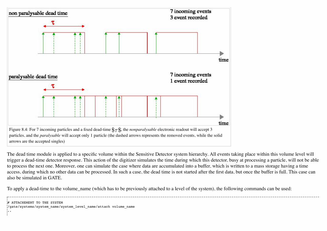
Figure 8.4: For 7 incoming particles and a fixed dead-time , the nonparalysable electronic readout will accept 3particles, and the paralysable will accept only 1 particle (the dashed arrows represents the removed events, while the solidarrows are the accepted singles)

The dead time module is applied to a specific volume within the Sensitive Detector system hierarchy. All events taking place within this volume level willtrigger a dead-time detector response. This action of the digitizer simulates the time during which this detector, busy at processing a particle, will not be ableto process the next one. Moreover, one can simulate the case where data are accumulated into a buffer, which is written to a mass storage having a timeaccess, during which no other data can be processed. In such a case, the dead time is not started after the first data, but once the buffer is full. This case canalso be simulated in GATE.

To apply a dead-time to the volume_name (which has to be previously attached to a level of the system), the following commands can be used:

# ATTACHEMENT TO THE SYSTEM /gate/systems/system_name/system_level_name/attach volume_name ..

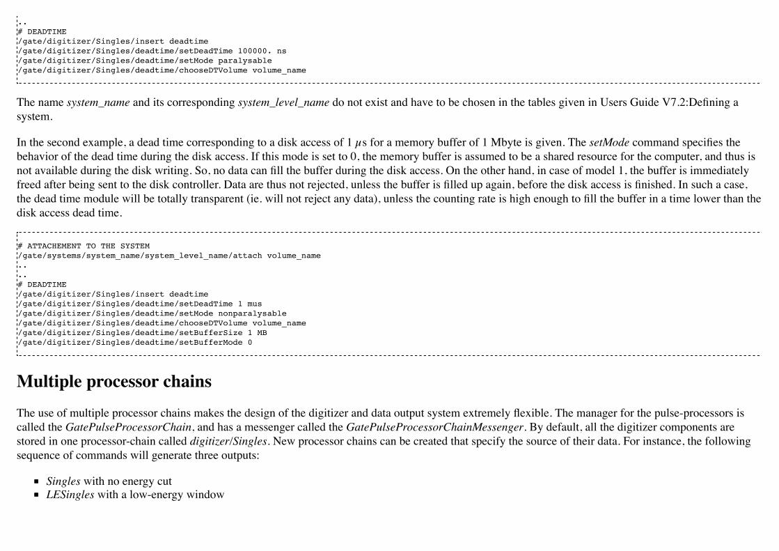
..# DEADTIME /gate/digitizer/Singles/insert deadtime /gate/digitizer/Singles/deadtime/setDeadTime 100000. ns /gate/digitizer/Singles/deadtime/setMode paralysable /gate/digitizer/Singles/deadtime/chooseDTVolume volume_name

The name system_name and its corresponding system_level_name do not exist and have to be chosen in the tables given in Users Guide V7.2:Defining asystem.

In the second example, a dead time corresponding to a disk access of 1 µs for a memory buffer of 1 Mbyte is given. The setMode command specifies thebehavior of the dead time during the disk access. If this mode is set to 0, the memory buffer is assumed to be a shared resource for the computer, and thus isnot available during the disk writing. So, no data can fill the buffer during the disk access. On the other hand, in case of model 1, the buffer is immediatelyfreed after being sent to the disk controller. Data are thus not rejected, unless the buffer is filled up again, before the disk access is finished. In such a case,the dead time module will be totally transparent (ie. will not reject any data), unless the counting rate is high enough to fill the buffer in a time lower than thedisk access dead time.

# ATTACHEMENT TO THE SYSTEM /gate/systems/system_name/system_level_name/attach volume_name....# DEADTIME /gate/digitizer/Singles/insert deadtime /gate/digitizer/Singles/deadtime/setDeadTime 1 mus /gate/digitizer/Singles/deadtime/setMode nonparalysable /gate/digitizer/Singles/deadtime/chooseDTVolume volume_name /gate/digitizer/Singles/deadtime/setBufferSize 1 MB /gate/digitizer/Singles/deadtime/setBufferMode 0

Multiple processor chainsThe use of multiple processor chains makes the design of the digitizer and data output system extremely flexible. The manager for the pulse-processors iscalled the GatePulseProcessorChain, and has a messenger called the GatePulseProcessorChainMessenger. By default, all the digitizer components arestored in one processor-chain called digitizer/Singles. New processor chains can be created that specify the source of their data. For instance, the followingsequence of commands will generate three outputs:

Singles with no energy cutLESingles with a low-energy window

HESingles with a high-energy window

For a standard PET (with BGO crystals), the components of the standard processor chain will consist in the following commands:

/gate/digitizer/Singles/insert adder /gate/digitizer/Singles/insert readout /gate/digitizer/Singles/readout/setDepth 1

To add the blurring filter to the "Single" branch:

/gate/digitizer/Singles/insert blurring /gate/digitizer/Singles/blurring/setResolution 0.26 /gate/digitizer/Singles/blurring/setEnergyOfReference 511. keV

The following commands create a low-energy chain branching from the output of "Singles" chain:

/gate/digitizer/name LESingles /gate/digitizer/insert singleChain /gate/digitizer/LESingles/setInputName Singles /gate/digitizer/LESingles/insert thresholder /gate/digitizer/LESingles/thresholder/setThreshold 50. keV /gate/digitizer/LESingles/insert upholder /gate/digitizer/LESingles/upholder/setUphold 350. keV

These next commands create a high-energy chain branching from the output of the "Singles" chain:

/gate/digitizer/name HESingles /gate/digitizer/insert singleChain /gate/digitizer/HESingles/setInputName Singles /gate/digitizer/HESingles/insert thresholder /gate/digitizer/HESingles/thresholder/setThreshold 350. keV /gate/digitizer/HESingles/insert upholder /gate/digitizer/HESingles/upholder/setUphold 650. keV

Coincidence sorter

The coincidence sorter searches, into the singles list, for pairs of coincident singles. Whenever two or more singles are found within a coincidence window,these singles are grouped to form a Coincidence event. Two methods are possible to find coincident singles within GATE. In the first method, when a singleis detected, it opens a new coincidence window, and search for a second single occurring during the length of the window. In this method, as long as thewindow opened by the first single is not closed, no other single can open its own coincidence window. In the second method, all singles open their owncoincidence window, and a logical OR is made between all the individual signals to find coincidences. The two methods are available in GATE, and can leadto slightly different results, for a given window width. A comparison of the difference of these two behaviors in a real case is sketched in figure 8.5.

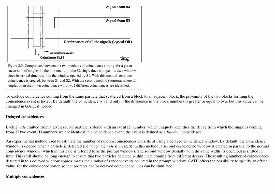
Figure 8.5: Comparison between the two methods of coincidence sorting, for a givensuccession of singles. In the first one (top), the S2 single does not open its own windowsince its arrival time is within the window opened by S1. With this method, only onecoincidence is created, between S1 and S2. With the second method (bottom), where allsingles open their own coincidence window, 2 different coincidences are identified.

To exclude coincidence coming from the same particle that scattered from a block to an adjacent block, the proximity of the two blocks forming thecoincidence event is tested. By default, the coincidence is valid only if the difference in the block numbers is greater or equal to two, but this value can bechanged in GATE if needed.

Delayed coincidences

Each Single emitted from a given source particle is stored with an event ID number, which uniquely identifies the decay from which the single is comingfrom. If two event ID numbers are not identical in a coincidence event, the event is defined as a Random coincidence.

An experimental method used to estimate the number of random coincidences consists of using a delayed coincidence window. By default, the coincidencewindow is opened when a particle is detected (i.e. when a Single is created). In this method, a second coincidence window is created in parallel to the normalcoincidence window (which in this case is referred to as the prompt window). The second window (usually with the same width) is open, but is shifted intime. This shift should be long enough to ensure that two particles detected within it are coming from different decays. The resulting number of coincidencesdetected in this delayed window approximates the number of random events counted in the prompt window. GATE offers the possibility to specify an offsetvalue, for the coincidence sorter, so that prompts and/or delayed coincidence lines can be simulated.

Multiple coincidences

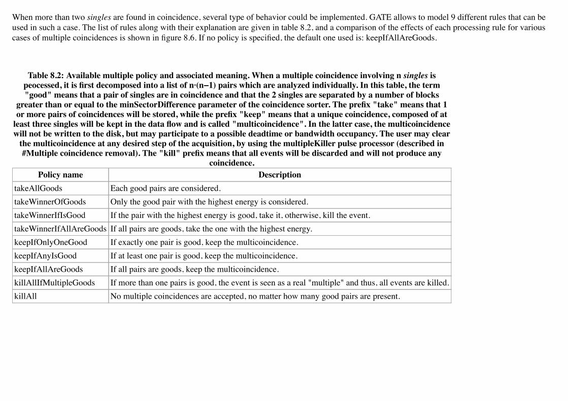
When more than two singles are found in coincidence, several type of behavior could be implemented. GATE allows to model 9 different rules that can beused in such a case. The list of rules along with their explanation are given in table 8.2, and a comparison of the effects of each processing rule for variouscases of multiple coincidences is shown in figure 8.6. If no policy is specified, the default one used is: keepIfAllAreGoods.

Table 8.2: Available multiple policy and associated meaning. When a multiple coincidence involving n singles ispeocessed, it is first decomposed into a list of n·(n−1) pairs which are analyzed individually. In this table, the term"good" means that a pair of singles are in coincidence and that the 2 singles are separated by a number of blocks

greater than or equal to the minSectorDifference parameter of the coincidence sorter. The prefix "take" means that 1or more pairs of coincidences will be stored, while the prefix "keep" means that a unique coincidence, composed of at

least three singles will be kept in the data flow and is called "multicoincidence". In the latter case, the multicoincidencewill not be written to the disk, but may participate to a possible deadtime or bandwidth occupancy. The user may clear

the multicoincidence at any desired step of the acquisition, by using the multipleKiller pulse processor (described in#Multiple coincidence removal). The "kill" prefix means that all events will be discarded and will not produce any

coincidence.Policy name Description

takeAllGoods Each good pairs are considered.takeWinnerOfGoods Only the good pair with the highest energy is considered.takeWinnerIfIsGood If the pair with the highest energy is good, take it, otherwise, kill the event.takeWinnerIfAllAreGoods If all pairs are goods, take the one with the highest energy.keepIfOnlyOneGood If exactly one pair is good, keep the multicoincidence.keepIfAnyIsGood If at least one pair is good, keep the multicoincidence.keepIfAllAreGoods If all pairs are goods, keep the multicoincidence.killAllIfMultipleGoods If more than one pairs is good, the event is seen as a real "multiple" and thus, all events are killed.killAll No multiple coincidences are accepted, no matter how many good pairs are present.

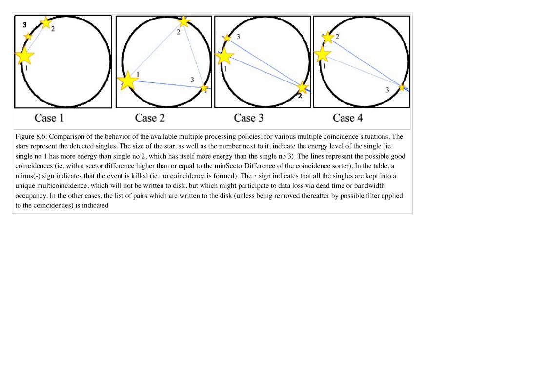
Figure 8.6: Comparison of the behavior of the available multiple processing policies, for various multiple coincidence situations. Thestars represent the detected singles. The size of the star, as well as the number next to it, indicate the energy level of the single (ie.single no 1 has more energy than single no 2, which has itself more energy than the single no 3). The lines represent the possible goodcoincidences (ie. with a sector difference higher than or equal to the minSectorDifference of the coincidence sorter). In the table, aminus(-) sign indicates that the event is killed (ie. no coincidence is formed). The ⋆ sign indicates that all the singles are kept into aunique multicoincidence, which will not be written to disk, but which might participate to data loss via dead time or bandwidthoccupancy. In the other cases, the list of pairs which are written to the disk (unless being removed thereafter by possible filter appliedto the coincidences) is indicated

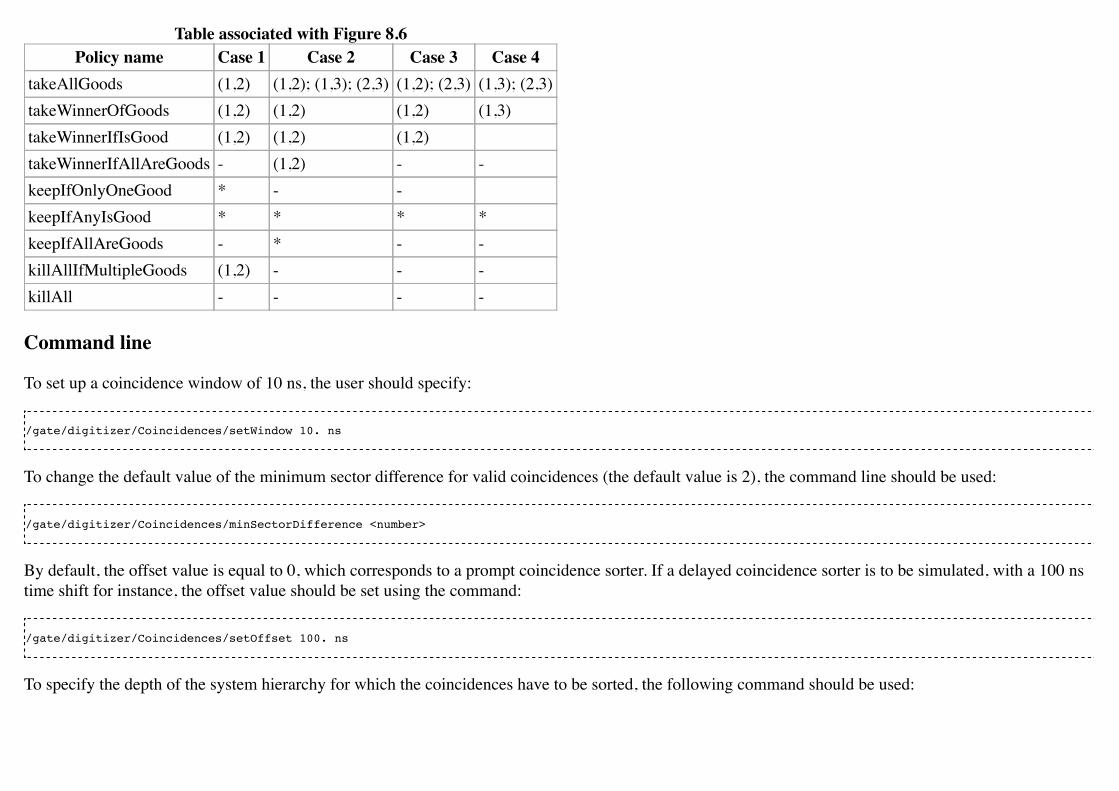
Table associated with Figure 8.6Policy name Case 1 Case 2 Case 3 Case 4

takeAllGoods (1,2) (1,2); (1,3); (2,3) (1,2); (2,3) (1,3); (2,3)takeWinnerOfGoods (1,2) (1,2) (1,2) (1,3)takeWinnerIfIsGood (1,2) (1,2) (1,2)takeWinnerIfAllAreGoods - (1,2) - -keepIfOnlyOneGood * - -keepIfAnyIsGood * * * *keepIfAllAreGoods - * - -killAllIfMultipleGoods (1,2) - - -killAll - - - -

Command line

To set up a coincidence window of 10 ns, the user should specify:

/gate/digitizer/Coincidences/setWindow 10. ns

To change the default value of the minimum sector difference for valid coincidences (the default value is 2), the command line should be used:

/gate/digitizer/Coincidences/minSectorDifference <number>

By default, the offset value is equal to 0, which corresponds to a prompt coincidence sorter. If a delayed coincidence sorter is to be simulated, with a 100 nstime shift for instance, the offset value should be set using the command:

/gate/digitizer/Coincidences/setOffset 100. ns

To specify the depth of the system hierarchy for which the coincidences have to be sorted, the following command should be used:

/gate/digitizer/Coincidences/setDepth <system's depth (1 by default)>

As explained in figure 8.5, there are two methods for building coincidences. The default one is the method 1. To switch to method 2, one should use:

/gate/digitizer/Coincidences/allPulseOpenCoincGate true

So when set to false (by default) the method 1 is chosen, and when set to true, this is the method 2. Be aware that the method 2 is experimental and notvalidated at all, so potentially containing non-reported bugs.

Finally, the rule to apply in case of multiple coincidences is specified as follows:

/gate/digitizer/Coincidences/setMultiplePolicy <policyName>

The default multiple policy is keepIfAllAreGoods.

Multiple coincidence sortersMultiple coincidence sorters can be used in GATE. To create a coincidence sorter, the sorter must be named and a location specified for the input data. In theexample below, three new coincidence sorters are created:

One with a very long coincidence window:

/gate/digitizer/name LongCoincidences /gate/digitizer/insert coincidenceSorter /gate/digitizer/LongCoincidences/setInputName Singles /gate/digitizer/LongCoincidences/setWindow 1000. ns

One for low-energy singles

/gate/digitizer/name LECoincidences /gate/digitizer/insert coincidenceSorter /gate/digitizer/LECoincidences/setWindow 10. ns /gate/digitizer/LECoincidences/setInputName LESingles

One for high-energy-singles

/gate/digitizer/name HECoincidences /gate/digitizer/insert coincidenceSorter /gate/digitizer/HECoincidences/setWindow 10. ns /gate/digitizer/HECoincidences/setInputName HESingles

A schematic view corresponding to this example is shown in figure 8.7.

Figure 8.7: Readout scheme produced by the listing from the sections

Coincidence processing and filtering

Coincidence pulse processors

Once the coincidences are identified, further processing can be applied to mimic count losses that may occur because of the acquisition limitations, such asdead time. Count loss may also be due to the limited bandwidth of wires or buffer capacities of the I/O interface. The modelling of such effects within GATEis explained below. Moreover, for PET scanners using a delayed coincidence line, data coming from the two types of coincidences (ie. prompts and delayed)can be processed by a unique coincidence sorter. If so, the rate of a coincidence type can affect the rate of the other. For instance, a prompt coincidence canproduce dead time which will hide a delayed coincidence. The prompt coincidence events can also saturate the bandwidth, so that the random events arepartially hidden.

The modelling of such effects consists in grouping the two different coincidence types into a unique one, which is then processed by a unique filter.

A coincidence pulse processor is a structure that contains the list of coincidence sources onto which a set of filters will be applied, along with the list offilters themselves. The order of the list of coincidence may impact the repartition of the data loss between the prompt and the delay lines. For example, if theline of prompt coincidences has priority over the line of delayed coincidences, then the events of the latter have more risk to be rejected by a possible bufferoverflow than those of the former. This kind of effects can be suppressed by specifying that, inside an event, all the coincidences arriving with the same timeflag are merged in a random order.

To implement a coincidence pulse processor merging two coincidence lines into one, and apply an XXX module followed by another YYY module on thetotal data flow, one should use the following commands, assuming that the two coincidence lines named prompts and delayed are already defined:

/gate/digitizer/name myCoincChain /gate/digitizer/insert coincidenceChain /gate/digitizer/myCoincChain/addSource prompts /gate/digitizer/myCoincChain/addSource delayed /gate/digitizer/myCoincChain/insert XXX# set parameter of XXX.... /gate/digitizer/myCoincChain/insert YYY# set parameter of YYY....

To specify that two coincidences arriving with the same time flag have to be processed in random order, one should use the command:

/gate/digitizer/myCoincChain/usePriority false

Coincidence dead time

The dead time for coincidences works in the same way as that acting on the singles data flow. The only difference is that, for the single dead time, one canspecify the hierarchical level to which the dead time is applied on (corresponding to the separation of detectors and electronic modules), while in thecoincidence dead time, the possibility to simulate separate coincidence units (which may exist) is not implemented. Apart from this limitation, the command

lines for coincidence dead time are identical to the ones for singles dead time, as described in #Pile-up. When more than one coincidence can occur for aunique GEANT4 event (if more than one coincidence line are added to the coincidence pulse processor, or if multiple coincidences are processed as manycoincidences pairs), then the user can specify that the whole event is kept or rejected, depending on the arrival time of the first coincidence. To do so, oneshould use the command line:

/gate/digitizer/myCoincChain/deadtime/conserveAllEvent true

Coincidence buffers

The buffer module for affecting coincidences uses exactly the same command lines and functionalities as the ones used for single pulse lists, and describedin section #Local efficiency.

Multiple coincidence removal

If the multiple coincidences are kept and not splitted into pairs (ie. if any of the keepXXX multiple coincidence policy is used), the multicoincidences couldparticipate to dataflow occupancy, but could not be written to the disk. Unless otherwise specified, any multicoincidence is then cleared from data just beforethe disk writing. If needed, this clearing could be performed at any former coincidence processing step, by inserting the multipleKiller module at therequired level. This module has no parameter and just kill the multicoincidence events. Multiple coincidences split into many pairs are not affected by thismodule and cannot be distinguished from the normal "simple" coincidences. To insert a multipleKiller, one has to use the syntax:

/gate/digitizer/myCoincChain/insert multipleKiller

Example of a digitizer settingHere, the digitizer section of a GATE macro file is analyzed line by line. The readout scheme produced by this macro, which is commented on below, isillustrated in Figure 8.8.

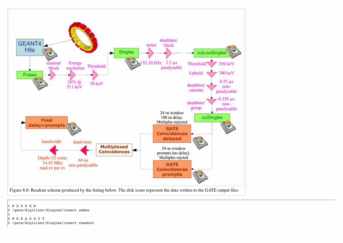
Figure 8.8: Readout scheme produced by the listing below. The disk icons represent the data written to the GATE output files

1 # A D D E R 2 /gate/digitizer/Singles/insert adder 3 4 # R E A D O U T 5 /gate/digitizer/Singles/insert readout

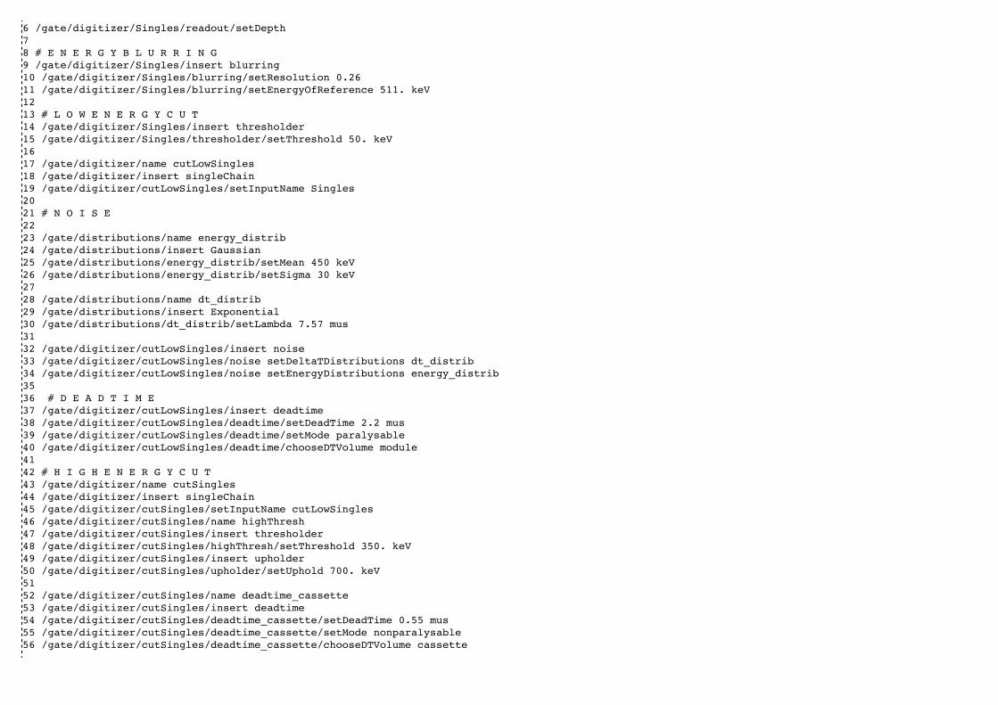
6 /gate/digitizer/Singles/readout/setDepth 78 # E N E R G Y B L U R R I N G 9 /gate/digitizer/Singles/insert blurring 10 /gate/digitizer/Singles/blurring/setResolution 0.26 11 /gate/digitizer/Singles/blurring/setEnergyOfReference 511. keV 12 13 # L O W E N E R G Y C U T14 /gate/digitizer/Singles/insert thresholder15 /gate/digitizer/Singles/thresholder/setThreshold 50. keV1617 /gate/digitizer/name cutLowSingles18 /gate/digitizer/insert singleChain19 /gate/digitizer/cutLowSingles/setInputName Singles20 21 # N O I S E22 23 /gate/distributions/name energy_distrib24 /gate/distributions/insert Gaussian 25 /gate/distributions/energy_distrib/setMean 450 keV 26 /gate/distributions/energy_distrib/setSigma 30 keV 27 28 /gate/distributions/name dt_distrib 29 /gate/distributions/insert Exponential 30 /gate/distributions/dt_distrib/setLambda 7.57 mus 3132 /gate/digitizer/cutLowSingles/insert noise 33 /gate/digitizer/cutLowSingles/noise setDeltaTDistributions dt_distrib 34 /gate/digitizer/cutLowSingles/noise setEnergyDistributions energy_distrib3536 # D E A D T I M E 37 /gate/digitizer/cutLowSingles/insert deadtime 38 /gate/digitizer/cutLowSingles/deadtime/setDeadTime 2.2 mus 39 /gate/digitizer/cutLowSingles/deadtime/setMode paralysable 40 /gate/digitizer/cutLowSingles/deadtime/chooseDTVolume module 4142 # H I G H E N E R G Y C U T 43 /gate/digitizer/name cutSingles 44 /gate/digitizer/insert singleChain 45 /gate/digitizer/cutSingles/setInputName cutLowSingles 46 /gate/digitizer/cutSingles/name highThresh 47 /gate/digitizer/cutSingles/insert thresholder 48 /gate/digitizer/cutSingles/highThresh/setThreshold 350. keV 49 /gate/digitizer/cutSingles/insert upholder 50 /gate/digitizer/cutSingles/upholder/setUphold 700. keV 51 52 /gate/digitizer/cutSingles/name deadtime_cassette 53 /gate/digitizer/cutSingles/insert deadtime 54 /gate/digitizer/cutSingles/deadtime_cassette/setDeadTime 0.55 mus 55 /gate/digitizer/cutSingles/deadtime_cassette/setMode nonparalysable 56 /gate/digitizer/cutSingles/deadtime_cassette/chooseDTVolume cassette

57 /gate/digitizer/cutSingles/name deadtime_group 58 /gate/digitizer/cutSingles/insert deadtime 59 /gate/digitizer/cutSingles/deadtime_group/setDeadTime 0.250 mus 60 /gate/digitizer/cutSingles/deadtime_group/setMode nonparalysable 61 /gate/digitizer/cutSingles/deadtime_group/chooseDTVolume group6263 64 # C O I N C I S O R T E R 65 65 /gate/digitizer/Coincidences/setInputName cutSingles 66 /gate/digitizer/Coincidences/setOffset 0. ns 67 /gate/digitizer/Coincidences/setWindow 24. ns 68 /gate/digitizer/Coincidences/minSectorDifference 3 69 70 /gate/digitizer/name delayedCoincidences 71 /gate/digitizer/insert coincidenceSorter 72 /gate/digitizer/delayedCoincidences/setInputName cutSingles 73 /gate/digitizer/delayedCoincidences/setOffset 100. ns 74 /gate/digitizer/delayedCoincidences/setWindow 24. ns 75 /gate/digitizer/delayedCoincidences/minSectorDifference 3 76 77 /gate/digitizer/name finalCoinc 78 /gate/digitizer/insert coincidenceChain 79 /gate/digitizer/finalCoinc/addInputName delay 80 /gate/digitizer/finalCoinc/addInputName Coincidences 81 /gate/digitizer/finalCoinc/usePriority true 82 /gate/digitizer/finalCoinc/insert deadtime 83 /gate/digitizer/finalCoinc/deadtime/setDeadTime 60 ns 84 /gate/digitizer/finalCoinc/deadtime/setMode nonparalysable 85 /gate/digitizer/finalCoinc/deadtime/conserveAllEvent true 86 /gate/digitizer/finalCoinc/insert buffer 87 /gate/digitizer/finalCoinc/buffer/setBufferSize 32 B 88 /gate/digitizer/finalCoinc/buffer/setReadFrequency 14.45 MHz 89 /gate/digitizer/finalCoinc/buffer/setMode 0

Lines 1 to 15: The branch named "Singles" contains the result of applying the adder, readout, blurring, and threshold (50 keV) modules.

Lines 17 to 20: A new branch (line 18) is defined, named "cutLowSingles" (line 17), which follows the "Singles" branch in terms of data flow (line 19).

Lines 21 to 35: Two distributions are created, which will be used for defining a background noise. The first distributions, named energy_distribution (line 23)is a Gaussian centered on 450 keV and of 30 keV standard deviation, while the second one is an exponential distribution with a power of 7.57 \mu s. Thesetwo distributions are used to add noise. The energy distribution of this source of noise is Gaussian, whileThe exponential distribution represents thedistribution of time interval between two consecutive noise events (lines 32-34).

Lines 37 to 40: A paralysable (line 39) dead time of 2.2 \mu s is applied on the resulting signal+noise events.

Lines 43 to 62: Another branch (line 44) named "cutSingles" (line 43) is defined. This branch contains a subset of the "cutLowSingles" branch (line 45)(after dead-time has been applied), composed of those events which pass through the 350 keV/700 keV threshold/uphold window (lines 46-50). In addition,the events tallied in this branch must pass the two dead-time cuts (lines 52 to 61) after the energy window cut.

Lines 65 to 68: The "default" coincidence branch consists of data taken from the output of the high threshold and two dead-time cuts ("cutSingles") (line 65).At this point, a 24 ns window with no delay is defined for this coincidence sorter.

Lines 70 to 75: A second coincidence branch is defined (line 71), which is named "delayedCoincidences". This branch takes its data from the same output("cutSingles"), but is defined by a delayed coincidence window of 24 ns, and a 100 ns delay (line 73).

Lines 77 to 89: The delayed and the prompts coincidence lines are grouped (lines 79-80). Between two coincidences coming from these two lines andoccuring within a given event, the priority is set to the delayed line, since it is inserted before the prompt line, and the priority is used (line 81). A non-paralysable dead time of 60 ns is applied on the delayed+prompt coincidences (lines 82-85). If more than one coincidence occur inside a given event, thedead time can kill all of them or none of them, depending on the arrival time of the first one. As a consequence, if a delay coincidence is immediatelyfollowed by a prompt coincidence due to the same photon, then, the former will not hide the latter (line 85). Finally, a memory buffer of 32 coincidences,read at a frequency of 14.45 MHz, in an event-by-event basis (line 89) is applied to the delayed+prompt sum (lines 86-89).

Digitizer optimizationIn GATE standard operation mode, primary particles are generated by the source manager, and then propagated through the attenuating geometry beforegenerating hits in the detectors, which feed into the digitizer chain. While this operation mode is suited for conventional simulations, it is inefficient whentrying to optimize the parameters of the digitizer chain. In this case, the user needs to compare the results obtained for different sets of digitizer parametersthat are based upon the same series of hits. Thus, repeating the particle generation and propagation stages of a simulation is unnecessary for tuning thedigitizer setting.

For this specific situation, GATE offers an operation mode dedicated to digitizer optimization, known as DigiGATE. In this mode, hits are no longergenerated: instead, they are read from a hit data-file (obtained from an initial GATE run) and are fed directly into the digitizer chain. By bypassing thegeneration and propagation stages, the computation speed is significantly reduced, thus allowing the user to compare various sets of digitizer parametersquickly, and optimize the model of the detection electronics. DigiGATE is further explained in chapter 13.

Angular Response Functions to speed-up planar or SPECT simulations

The ARF is a function of the incident photon direction and energy and represents the probability that a photon will either interact with or pass through thecollimator, and be detected at the intersection of the photon direction vector and the detection plane in an energy window of interest. The use of ARF cansignificantly speed up planar or SPECT simulations. The use of this functionality involves 3 steps.

Calculation of the data needed to derive the ARF tables

In this step, the data needed to generate the ARF tables are computed from a rectangular source located at the center of FOV. The SPECT head is duplicatedtwice and located at roughly 30 cm from the axial axis.

The command needed to compute the ARF data is:

/gate/systems/SPECThead/arf/setARFStage generateData

The ARF data are stored in ROOT format as specified by the GATE command output:

/gate/output/arf/setFileName testARFdata

By default the maximum size of a ROOT file is 1.8 Gbytes. Once the file has reached this size, ROOT automatically closes it and opens a new file nametestARFdata_1.root. When this file reaches 1.8 Gb, it is closed and a new file testARFdata_2.root is created etc. A template macro file is provided inhttps://github.com/OpenGATE/GateContrib/blob/master/imaging/ARF/generateARFdata.mac which illustrates the use of the commands listed before.

Computation of the ARF tables from the simulated data

Once the required data are stored in ROOT files, the ARF tables can be calculated and stored in a binary file:

/gate/systems/SPECThead/arf/setARFStage computeTables

The digitizer parameters needed for the computation of the ARF table are defined by:

/gate/systems/SPECThead/ARFTables/setEnergyDepositionThreshHold 328. keV/gate/systems/SPECThead/ARFTables/setEnergyDepositionUpHold 400. keV/gate/systems/SPECThead/ARFTables/setEnergyResolution 0.10/gate/systems/SPECThead/ARFTables/setEnergyOfReference 140. keV

In this example, we shot photons with 364.5 keV as kinetic energy. We chose an energy resolution of 10% @ 140 keV and the energy window was set to[328-400] keV. The simulated energy resolution at an energy Edep will be calculated by:

where Edep is the photon deposited energy.

If we want to discard photons which deposit less than 130 keV, we may use:

/gate/systems/SPECThead/setEnergyDepositionThreshHold 130. keV

The ARF tables depend strongly on the distance from the detector to the source used in the previous step. The detector plane is set to be the half-middle planof the detector part of the SPECT head. In our example, the translation of the SPECT head was 34.5 cm along the X direction (radial axis), the detector was2 cm wide along X and its center was located at x = 1.5 cm with respect to the SPECThead frame. This is what we call the detector plane (x = 1.5 cm) so thedistance from the source to the detector plane is 34.5 + 1.5 = 36 cm.

# DISTANCE FROM SOURCE TO DETECTOR PLANE TAKEN TO BE THE PLANE HALF-WAY THROUGH THE CRYSTAL RESPECTIVELY TO THE SPECTHEAD FRAME : here it is 34.5 cm + 1.5 cm/gate/systems/SPECThead/ARFTables/setDistanceFromSourceToDetector 36 cm

The tables are then computed from a text file which contains information regarding the incident photons called ARFData.txt which is provided inhttps://github.com/OpenGATE/GateContrib/tree/master/imaging/ARF

# NOW WE ARE READY TO COMPUTE THE ARF TABLES/gate/systems/SPECThead/ARFTables/ComputeTablesFromEnergyWindows ARFData.txt

The text file reads like this:

# this file contains all the energy windows computed during first step# with their associated root files# it has to be formatted the following way# [Emin,Emax] is the energy window of the incident photons# the Base FileName is the the name of the root files name.root, name_1.root name_2.root ...# the number of these files has to be given as the last parameter## enter the data for each energy window# Incident Energy Window: Emin - Emax (keV) | Root FileName | total file number 0. 365. test1head 20

Here we have only one incident energy window for which we want to compute the corresponding ARF tables. The data for this window are stored inside 20files whose base file name is test1head. These ARF data files were generated from the first step and were stored under the names of test1head.root,test1head_1.root ... test1head_19.root.

Finally the computed tables are stored to a binary file:

/gate/systems/SPECThead/ARFTables/list# SAVE ARF TABLES TO A BINARY FILE FOR PRODUCTION USE/gate/systems/SPECThead/ARFTables/saveARFTablesToBinaryFile ARFSPECTBench.bin

Use of the ARF tables

The command to tell GATE to use ARF tables is:

/gate/systems/SPECThead/arf/setARFStage useTables

The ARF sensitive detector is attached to the SPECThead:

/gate/SPECThead/attachARFSD

These tables are loaded from binary files with:

/gate/systems/SPECThead/ARFTables/loadARFTablesFromBinaryFile ARFTables.bin

Multi-system approaches: how to use more than one system in one simuation set-up ?Singles arriving from different systems request different treatment in the digitizer. So we have to use multiple digitizer chains and to separate between thesessingles according to their systems.

SystemFilter

The systemFilter module separates between the singles coming from systems. This module have one parameter which is the name of the system.

/gate/digitizer/SingleChain/insert systemFilter /gate/digitizer/SingleChain/systemFilter/selectSystem SystemName

SingleChain is the singles chain, Singles by default, and SystemName is the name of the selected system.

Suppose that we have two systems with the names “cylindricalPET” and “Scanner_1”, so to select singles in cylindricalPET system we use:

/gate/digitizer/Singles/insert systemFilter /gate/digitizer/Singles/systemFilter/selectSystem cylindricalPET

Note we didn't insert a singles chain because we have the default chain “Singles”, on the other side for “ Scanner_1” we to insert a new singles chain“Singles_S1 ”:

/gate/digitizer/name Singles_S1 /gate/digitizer/insert singleChain

Then we insert the system filter.

/gate/digitizer/Singles_S1/insert systemFilter /gate/digitizer/Singles_S1/systemFilter/selectSystem Scanner_1

How to manage the coincidence sorter with more than one system: the Tri Coincidence Sorter approach

The aim of this module is to obtain the coincidence between coincidence pulses and singles of another singles chain (between TEP camera and scanner forexample). In this module we search the singles, of the concerned singles chain, which are in coincidence with the coincidence pulses according to a timewindow. In fact, this module, from the point of view of the code, is coincidence pulses processor. So we have a coincidence chain as input with a singleschain. We have also to define a time window to search the coincident coincidence-singles within this window. We test the time difference between theaverage time of the tow singles of the coincidence pulse and the time of every single of the singles chain in question. We have as output of this module twotrees of ROOT: one tree contain the coincidences which have at first one coincident single with every one of them. The second tree contain the coincident

singles and it is generated automatically with name of coincidence tree+”CSingles”. For example if we call the coincidence “triCoinc”, so the name of thesingles tree will be “ triCoincCSingles”. This singles tree contain the same branches as any singles tree with an additional branch named “triCID” from (tricoincidence ID) and it has the same value for all singles which are in coincidence with one coincidence pulse.

In this module we store the singles event by event in a singles buffer that have a semi-constant size that the user can adjust. When we have a coincidencepulse we compare between the average time of this coincidence pulse and the time of each single pulse in the buffer. When we have coincident singles withthe coincidence pulse, we store them in two trees as mentioned above.

Define the classical coincidence sorter applied on the cylindrical PET system:

/gate/digitizer/Coincidences/setWindow 30. ns

Define now a "coincidenceChain" where you will plug the first coincidence sorter (named 'Coincidences' in that case):

/gate/digitizer/name TriCoinc/gate/digitizer/insert coincidenceChain/gate/digitizer/TriCoinc/addInputName Coincidences

Finally, we call the 'triCoincProcessor' module and we plug on it the second system which define in that case by the 'Singles_S1' chain:

/gate/digitizer/TriCoinc/insert triCoincProcessor/gate/digitizer/TriCoinc/triCoincProcessor/setSinglesPulseListName Singles_S1/gate/digitizer/TriCoinc/triCoincProcessor/setWindow 15 ns/gate/digitizer/TriCoinc/triCoincProcessor/setSinglesBufferSize 40

Retrieved from "http://wiki.opengatecollaboration.org/index.php?title=Users_Guide_V8.0:Digitizer_and_readout_parameters&oldid=906"


Users Guide V8.0:Data outputFrom Wiki OpenGATE

In GATE, there are several types of output format, which can be enabled. By default all outputs are disabled and moreover there is no default output filename. You _must_ give a file name, otherwise the output module will be automatically disabled.

All the output commands must always be written after the initialization line :

/gate/output/...

Contents1 ASCII and binary outputs

1.1 Description of the ASCII(binary) file content1.1.1 Hits file : gateHits.dat(.bin)1.1.2 Singles files : gateSingles.dat(.bin)1.1.3 Coincidences files : gateCoincidences.dat(.bin)

1.2 Selection of the variables in Singles/Coincidences ASCII and binary outputs1.3 Large files: automatic file swap1.4 What is the file gateRun.dat(.bin) ?

2 Root output2.1 Using TBrowser To Browse ROOT Objects2.2 How to merge Root files ?2.3 How to analyze the Root output2.4 Writing a counter in ROOT2.5 Draw all ROOT tree branches in a postscript file2.6 Convert a ROOT file to a text file2.7 The ROOT online plotter

3 Interfile output of projection set3.1 Reading an interfile image with ImageJ3.2 Reading an interfile image with IDL

4 Sinogram output5 Ecat7 output

5.1 Installation5.2 Data reduction5.3 Sinogram file

6 LMF output6.1 Limitations

7 Image CT output

ASCII and binary outputsThe GateToASCII/GateToBinary classes enable the ASCII/binary file output. It allows you to process your raw data with your own tools. On the other hand,this output is not compressed and the output files are very large. If the ASCII/binary files are not needed for analysis, it is strongly recommended not usingthis output to speed up the simulation and save space.

/gate/output/ascii(binary)/enable/gate/output/ascii/setFileName test

# enable ascii(binary) output for hits/gate/output/ascii(binary)/setOutFileHitsFlag 1

# enable ascii(binary) output for Singles (end of digitizer chain)/gate/output/ascii(binary)/setOutFileSinglesFlag 1

# enable ascii(binary) output for coincidences/gate/output/ascii(binary)/setOutFileCoincidencesFlag 1

# enable ascii(binary) output for singles (after a digitizer module)/gate/output/ascii(binary)/setOutFileSingles< name of the digitizer module >Flag 1

The names of the digitizer module are : Adder, Readout, Spblurring, Blurring, Thresholder, Upholder. Their actions are explained in Users GuideV7.2:Digitizer and readout parameters.

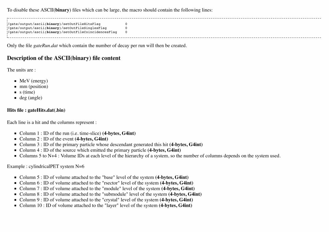
To disable these ASCII(binary) files which can be large, the macro should contain the following lines:

/gate/output/ascii(binary)/setOutFileHitsFlag 0/gate/output/ascii(binary)/setOutFileSinglesFlag 0/gate/output/ascii(binary)/setOutFileCoincidencesFlag 0

Only the file gateRun.dat which contain the number of decay per run will then be created.

Description of the ASCII(binary) file content

The units are :

MeV (energy)mm (position)s (time)deg (angle)

Hits file : gateHits.dat(.bin)

Each line is a hit and the columns represent :

Column 1 : ID of the run (i.e. time-slice) (4-bytes, G4int)Column 2 : ID of the event (4-bytes, G4int)Column 3 : ID of the primary particle whose descendant generated this hit (4-bytes, G4int)Column 4 : ID of the source which emitted the primary particle (4-bytes, G4int)Columns 5 to N+4 : Volume IDs at each level of the hierarchy of a system, so the number of columns depends on the system used.

Example : cylindricalPET system N=6

Column 5 : ID of volume attached to the "base" level of the system (4-bytes, G4int)Column 6 : ID of volume attached to the "rsector" level of the system (4-bytes, G4int)Column 7 : ID of volume attached to the "module" level of the system (4-bytes, G4int)Column 8 : ID of volume attached to the "submodule" level of the system (4-bytes, G4int)Column 9 : ID of volume attached to the "crystal" level of the system (4-bytes, G4int)Column 10 : ID of volume attached to the "layer" level of the system (4-bytes, G4int)

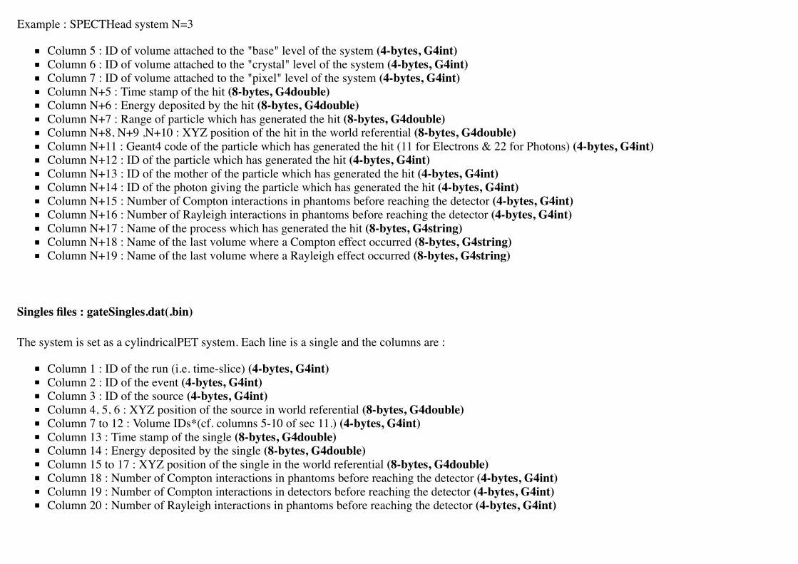
Example : SPECTHead system N=3

Column 5 : ID of volume attached to the "base" level of the system (4-bytes, G4int)Column 6 : ID of volume attached to the "crystal" level of the system (4-bytes, G4int)Column 7 : ID of volume attached to the "pixel" level of the system (4-bytes, G4int)Column N+5 : Time stamp of the hit (8-bytes, G4double)Column N+6 : Energy deposited by the hit (8-bytes, G4double)Column N+7 : Range of particle which has generated the hit (8-bytes, G4double)Column N+8, N+9 ,N+10 : XYZ position of the hit in the world referential (8-bytes, G4double)Column N+11 : Geant4 code of the particle which has generated the hit (11 for Electrons & 22 for Photons) (4-bytes, G4int)Column N+12 : ID of the particle which has generated the hit (4-bytes, G4int)Column N+13 : ID of the mother of the particle which has generated the hit (4-bytes, G4int)Column N+14 : ID of the photon giving the particle which has generated the hit (4-bytes, G4int)Column N+15 : Number of Compton interactions in phantoms before reaching the detector (4-bytes, G4int)Column N+16 : Number of Rayleigh interactions in phantoms before reaching the detector (4-bytes, G4int)Column N+17 : Name of the process which has generated the hit (8-bytes, G4string)Column N+18 : Name of the last volume where a Compton effect occurred (8-bytes, G4string)Column N+19 : Name of the last volume where a Rayleigh effect occurred (8-bytes, G4string)

Singles files : gateSingles.dat(.bin)

The system is set as a cylindricalPET system. Each line is a single and the columns are :

Column 1 : ID of the run (i.e. time-slice) (4-bytes, G4int)Column 2 : ID of the event (4-bytes, G4int)Column 3 : ID of the source (4-bytes, G4int)Column 4, 5, 6 : XYZ position of the source in world referential (8-bytes, G4double)Column 7 to 12 : Volume IDs*(cf. columns 5-10 of sec 11.) (4-bytes, G4int)Column 13 : Time stamp of the single (8-bytes, G4double)Column 14 : Energy deposited by the single (8-bytes, G4double)Column 15 to 17 : XYZ position of the single in the world referential (8-bytes, G4double)Column 18 : Number of Compton interactions in phantoms before reaching the detector (4-bytes, G4int)Column 19 : Number of Compton interactions in detectors before reaching the detector (4-bytes, G4int)Column 20 : Number of Rayleigh interactions in phantoms before reaching the detector (4-bytes, G4int)

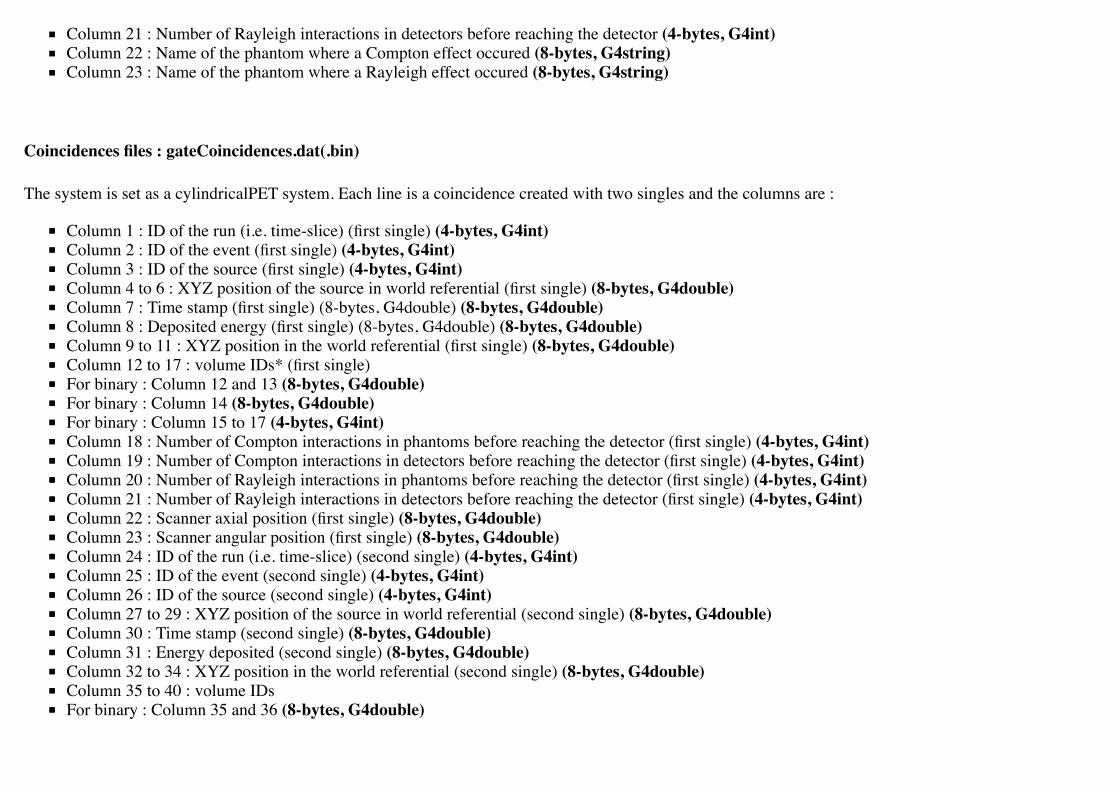
Column 21 : Number of Rayleigh interactions in detectors before reaching the detector (4-bytes, G4int)Column 22 : Name of the phantom where a Compton effect occured (8-bytes, G4string)Column 23 : Name of the phantom where a Rayleigh effect occured (8-bytes, G4string)

Coincidences files : gateCoincidences.dat(.bin)

The system is set as a cylindricalPET system. Each line is a coincidence created with two singles and the columns are :

Column 1 : ID of the run (i.e. time-slice) (first single) (4-bytes, G4int)Column 2 : ID of the event (first single) (4-bytes, G4int)Column 3 : ID of the source (first single) (4-bytes, G4int)Column 4 to 6 : XYZ position of the source in world referential (first single) (8-bytes, G4double)Column 7 : Time stamp (first single) (8-bytes, G4double) (8-bytes, G4double)Column 8 : Deposited energy (first single) (8-bytes, G4double) (8-bytes, G4double)Column 9 to 11 : XYZ position in the world referential (first single) (8-bytes, G4double)Column 12 to 17 : volume IDs* (first single)For binary : Column 12 and 13 (8-bytes, G4double)For binary : Column 14 (8-bytes, G4double)For binary : Column 15 to 17 (4-bytes, G4int)Column 18 : Number of Compton interactions in phantoms before reaching the detector (first single) (4-bytes, G4int)Column 19 : Number of Compton interactions in detectors before reaching the detector (first single) (4-bytes, G4int)Column 20 : Number of Rayleigh interactions in phantoms before reaching the detector (first single) (4-bytes, G4int)Column 21 : Number of Rayleigh interactions in detectors before reaching the detector (first single) (4-bytes, G4int)Column 22 : Scanner axial position (first single) (8-bytes, G4double)Column 23 : Scanner angular position (first single) (8-bytes, G4double)Column 24 : ID of the run (i.e. time-slice) (second single) (4-bytes, G4int)Column 25 : ID of the event (second single) (4-bytes, G4int)Column 26 : ID of the source (second single) (4-bytes, G4int)Column 27 to 29 : XYZ position of the source in world referential (second single) (8-bytes, G4double)Column 30 : Time stamp (second single) (8-bytes, G4double)Column 31 : Energy deposited (second single) (8-bytes, G4double)Column 32 to 34 : XYZ position in the world referential (second single) (8-bytes, G4double)Column 35 to 40 : volume IDsFor binary : Column 35 and 36 (8-bytes, G4double)

For binary : Column 37 (8-bytes, G4double)For binary : Column 38 to 40 (4-bytes, G4int)

The number of different volumeIDs depends on the complexity of the system geometry (6 IDs for cylindricalPET system, 3 for ECAT system, ...). Then, thenumber of column of your ASCII file is not constant, but system-dependent.

Column 41 : Number of Compton interactions in phantoms before reaching the detector (second single) (4-bytes, G4int)Column 42 : Number of Compton interactions in detectors before reaching the detector (second single) (4-bytes, G4int)Column 41 : Number of Rayleigh interactions in phantoms before reaching the detector (second single) (4-bytes, G4int)Column 42 : Number of Rayleigh interactions in detectors before reaching the detector (second single) (4-bytes, G4int)Column 45 : Scanner axial position (second single) (8-bytes, G4double)Column 46 : Scanner angular position (second single) (8-bytes, G4double)

Selection of the variables in Singles/Coincidences ASCII and binary outputs

The user can select which variables he/she wants in the ASCII(binary) file. The mechanism is based on a series of 0/1, one for each variable. By default allvariables are enabled, but one can choose to enable only some of the variables listed in 10.4.1.

/gate/output/ascii(binary)/setCoincidenceMask 1 0 1 0 1 1/gate/output/ascii(binary)/setSingleMask 0 0 1 1

Note: the VolumeID variables are enabled/disabled together, as a group. The component of the 3D vectors, instead, like the positions (components x,y,z), areenabled/disabled one by one.

Large files: automatic file swap

When a user defined limit is reached by the Coincidence or Single ASCII(binary) output file, by default Gate closes the file and opens another one with thesame name but a suffix _1 (and then _2, and so on). By default the file limit is set to 2000000000 bytes. One can change the number of bytes with acommand like

/gate/output/ascii(binary)/setOutFileSizeLimit 30000

If the value is < 10000, no file swapping is made (to avoid creating thousands of files by mistake).

For example, if one does not have any limit in the Operating System, one can put the number to 0, and there will be only one large (large) file at the end.

In case of high statistics applications, one might consider enabling only the ROOT output (see #The Root output), which contains the same information asthe binary one, but automatically compressed and ready for analysis.

What is the file gateRun.dat(.bin) ?

This file is the list of the number of decays generated by the source for each run (one by line). The Output manager is called for each event, even if theparticle(s) of the decay do not reach the detector. Note that the number of processed decays can be slighly different from the expected number

where is the activity and is the time of the acquisition, due to the random character of the decay which governs the event generation(Poisson law). Gate generates the time delay from the previous event, if it is out of the time slice it stops the event processing for the current time slice and ifneeded it starts a new time slice.

Root output

/gate/output/root/enable/gate/output/root/setFileName FILE_NAME

which will provide you with a FILE_NAME.root file. By default, this root file will contain : 2 Trees for SPECT systems (Hits and Singles) or 3 Trees forPET systems (Coincidences, Hits and Singles) in which several variables are stored.

If needed, and for a matter of file size, you could choose not to generate all trees. In this case, just add the following lines in your macro :

/gate/output/root/setRootHitFlag 0/gate/output/root/setRootSinglesFlag 0/gate/output/root/setRootCoincidencesFlag 0/gate/output/root/setRootNtupleFlag 0

By turning to 1 (or 0) one of this tree flag, you will fill (or not) the given tree.

In a debug mode, it can be useful to store in a Tree the informations after the action of one particular module of the digitizer chain. The following flags existto turn on or off these intermediate trees.

/gate/output/root/setOutFileSinglesAdderFlag 0

/gate/output/root/setOutFileSinglesReadoutFlag 0/gate/output/root/setOutFileSinglesSpblurringFlag 0/gate/output/root/setOutFileSinglesBlurringFlag 0/gate/output/root/setOutFileSinglesThresholderFlag 0/gate/output/root/setOutFileSinglesUpholderFlag 0

If you want to disable the whole ROOT output, just do not call it, or use the following command :

/gate/output/root/disable

Using TBrowser To Browse ROOT Objects

The ROOT graphical user interface TBrowser is a useful tool to interactively inspect and visualize produced simulation data.

Since Gate 8.0 new branches are included in the ROOT Hits Tree: trackLength, trackLocalTime, momDirX, momDirY and momDirZ. The additionalinformation that is now available can be used for applications like timing resolution and surface treatment studies of scintillation crystals when surfaces aredefined (see Users_Guide_V8.0:Generating_and_tracking_optical_photons#Defining_surfaces).

When launching ROOT with the command in a terminal :

root FILE_NAME.rootroot [1] TBrowser t

you can easily see the content of your ROOT data file.

Select desired outputfile (.root).

The trees (Hits, Singles etc.) will be filled according to the flags set to 1 in your .mac-file.

/gate/output/root/setRootHitFlag 1

Figure 10.1: Root file test.rootin the TBrowser.

The Hits tree is opened and shows many branches. Select a tree. Either double click on each branch to see histogrammed/plotted data or use root commandslike

Hits->Draw( “posX:posY:posZ”)

This command plots the position of Hits in 3D.

Figure 10.2: Position of Hits in 3D.

Add conditions to specify your histogram e.g.

Hits->Draw(“posX:posY:posZ”,”PDGEncoding==22”)

This command plots the position of Hits that are optical photons(PDGEncoding=22) in 3D.

Hits->Draw(“posX:posY:posZ”,”PDGEncoding==22 && time<=1 ”)

Multiple conditions can be added e.g.: 3D position of optical photons in the first second of the simulation.

PDGEncoding (Particle Data Group): The type of particle can be obtained (e.g.: “0” optical photon; “22” gamma particle; complete list:http://geant4.cern.ch/G4UsersDocuments/UsersGuides/ForApplicationDeveloper/html/TrackingAndPhysics/particle.html).

trackLocalTime[s]: (available starting Gate 8.0) The time that it takes a particle to complete a track.

It correlates directly to the trackLength according to the following formula:

time[s]: The absolute time of a hit in the sensitive detector.

stepLength[mm]: The distance between two interactions of a particle (e.g.: distance between a gamma particle entering a sensitive volume and beingscattered)trackLength[mm]: (available starting Gate 8.0) The total distance of one particle often including multiple steps. Can also be derived by thetrackLocalTime.

Figure 10.3: trackLength

momDirX,Y,Z: (available starting Gate 8.0) The momentum direction of a detected/absorbed particle in the sensitive detector consisting of threecomponents that make a 3D vector.

Use

Hits->Draw(“momDirX: momDirY: momDirZ”)

to look at vectors in 3D.

Figure 10.3: Momentum direction of particles.

processName: The process by which the particle ended its path in the sensitive detector (e.g.: Transportation (“T”), Optical Absorption(“O”),Comptonscatter(”C”), PhotoElectric(“P”), RaleighScattering(“R”)). You might be interested in distinguishing between particles that are detected at thedetector(“T”) and those that were absorbed(“O”). A particle that undergoes Comptonscatter(“C”) is counted as two hits when it splits up.

(for more information http://www-root.fnal.gov/root/GettingStarted/GettingStarted.htm)

How to merge Root files ?

Two or more Root files can be merged into one single file by using the hadd utility on the command line :

hadd MergedFile.root file1.root file2.root ... fileN.root

How to analyze the Root output

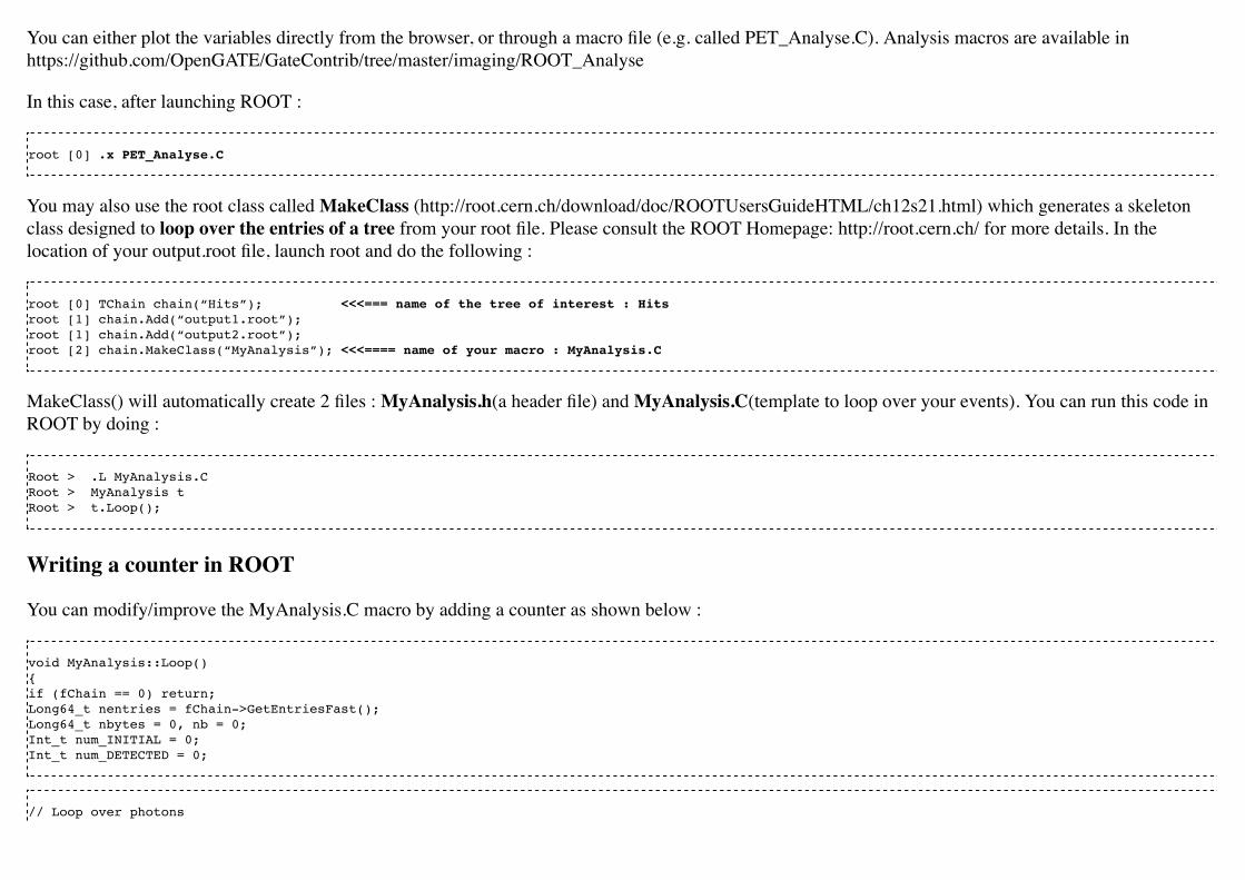
You can either plot the variables directly from the browser, or through a macro file (e.g. called PET_Analyse.C). Analysis macros are available inhttps://github.com/OpenGATE/GateContrib/tree/master/imaging/ROOT_Analyse

In this case, after launching ROOT :

root [0] .x PET_Analyse.C

You may also use the root class called MakeClass (http://root.cern.ch/download/doc/ROOTUsersGuideHTML/ch12s21.html) which generates a skeletonclass designed to loop over the entries of a tree from your root file. Please consult the ROOT Homepage: http://root.cern.ch/ for more details. In thelocation of your output.root file, launch root and do the following :

root [0] TChain chain(“Hits”); <<<=== name of the tree of interest : Hitsroot [1] chain.Add(“output1.root”);root [1] chain.Add(“output2.root”);root [2] chain.MakeClass(“MyAnalysis”); <<<==== name of your macro : MyAnalysis.C

MakeClass() will automatically create 2 files : MyAnalysis.h(a header file) and MyAnalysis.C(template to loop over your events). You can run this code inROOT by doing :

Root > .L MyAnalysis.CRoot > MyAnalysis tRoot > t.Loop();

Writing a counter in ROOT

You can modify/improve the MyAnalysis.C macro by adding a counter as shown below :

void MyAnalysis::Loop(){if (fChain == 0) return;Long64_t nentries = fChain->GetEntriesFast();Long64_t nbytes = 0, nb = 0;Int_t num_INITIAL = 0;Int_t num_DETECTED = 0;

// Loop over photons

for (Long64_t jentry=0; jentry Long64_t ientry = LoadTree(jentry);if (ientry < 0) break;nb = fChain->GetEntry(jentry); nbytes += nb;num_INITIAL++; // number of photons in the treeif(HitPos_Y == 0.3) <== here you could apply some cuts which are analysis dependentnum_DETECTED++;}}// End Loop over the entries.

// You can print some results on the screen :std::cout<<"***************************** Results *****************************" << std::endl;std::cout<<"Number of Generated Photons: " << num_INITIAL << std::endl;std::cout<<"Number of Detected Photons: " << num_DETECTED << std::endl;

Draw all ROOT tree branches in a postscript file

If you look at the GATE code optical example directory (https://github.com/OpenGATE/GateContrib/tree/master/imaging/Optical), you will see a macronamed DrawBranches.C. If you modify it so it points to your root file and execute it in root : root> .x DrawBranches.C This will draw/plot all the branchesof your tree into a postscript file. That might be helpful.

Convert a ROOT file to a text file

This link shows how to convert the data in a root file to a text file for further analysis: http://root.cern.ch/phpBB3/viewtopic.php?f=3&t=16590

// Name this file "dump.cxx" and use as:// root [0] .x dump.cxx(); > dump.txt// Produces "dump.txt" and "dump.xml" files.

void dump(const char *fname = "dna.root", const char *nname = "ntuple”) // <=== If needed, change this line.{if (!fname || !(*fname) || !nname || !(*nname)) return; // just a precaution TFile *f = TFile::Open(fname, "READ");if (!f) return; // just a precaution TTree *t; f->GetObject(nname, t);if (!t) { delete f; return; } // just a precaution // See:// http://root.cern.ch/root/html/TTreePlayer.html#TTreePlayer:Scan// http://root.cern.ch/root/html/TTree.html#TTree:Scan

t->SetScanField(0);t->Scan("*"); // See:// http://root.cern.ch/root/html/TObject.html#TObject:SaveAst->SaveAs("dump.xml");// t->SaveAs(TString::Format("%s.xml", nname)); delete f; // no longer needed (automatically deletes "t")}

The ROOT online plotter

GATE provides a very convenient tool called the online plotter, which enables online display of several variables. This online analysis is available even ifthe root output is disabled in your macro, for instance because the user does not want to save a large root file. But Gate have to be compiled with certainoptions to have this output available.The online plotter can be easily used with the following macro :

/gate/output/plotter/enable/gate/output/plotter/showPlotter /gate/output/plotter/setNColumns 2 <=== sets the number of display windows to be used /gate/output/plotter/setPlotHeight 250/gate/output/plotter/setPlotWidth 300/gate/output/plotter/addPlot hist Ion_decay_time_s <=== plots an histogram previously defined in GATE /gate/output/plotter/addPlot hist Positron_Kinetic_Energy_MeV <=== plots a variable from one of the GATE trees/gate/output/plotter/addPlot tree Singles comptonPhantom/gate/output/plotter/addPlot tree Coincidences energy1/gate/output/plotter/listPlots

Figure 10.2 presents an example of online plotter, obtained with the above macro.

Figure 10.2: The Online Plotter

Interfile output of projection setThe Interfile format is especially suited for acquisition protocol using a multiple headed rotating gamma camera. The total description of the Interfilev3.3format can be found on the Interfile website: http://www.medphys.ucl.ac.uk/interfile/index.htm.

When images are acquired in multiple windows (e.g. energy windows, time windows, multiple heads), the images are recorded according to the order inwhich the corresponding keys are defined. Thus if multiple energy windows are used, all image data for the first window must be given first, followed by theimage data for the second window, etc. This loop structure is defined in the Interfile syntax by the use of the 'for' statement. Two files are created when using

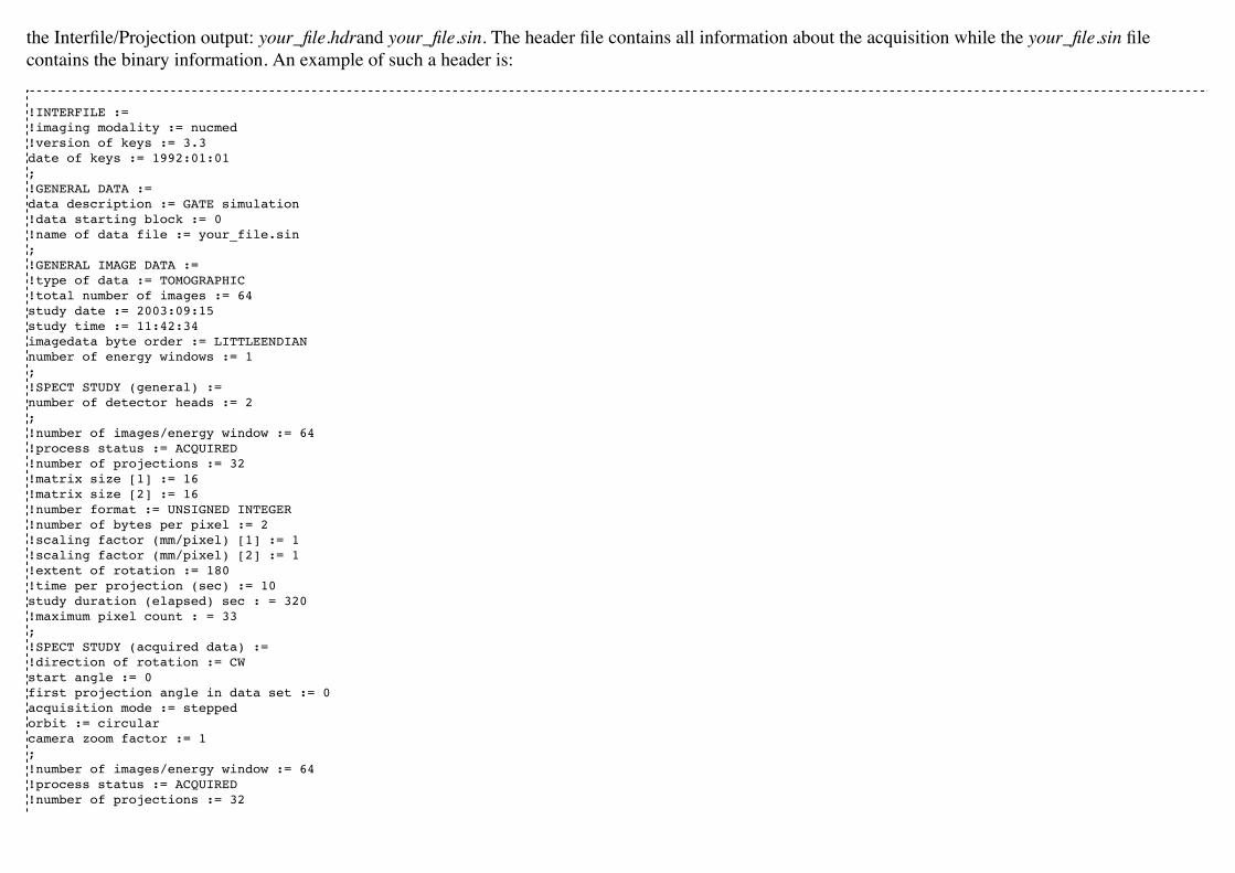
the Interfile/Projection output: your_file.hdrand your_file.sin. The header file contains all information about the acquisition while the your_file.sin filecontains the binary information. An example of such a header is:

!INTERFILE :=!imaging modality := nucmed!version of keys := 3.3date of keys := 1992:01:01;!GENERAL DATA :=data description := GATE simulation!data starting block := 0!name of data file := your_file.sin;!GENERAL IMAGE DATA :=!type of data := TOMOGRAPHIC!total number of images := 64study date := 2003:09:15study time := 11:42:34imagedata byte order := LITTLEENDIANnumber of energy windows := 1;!SPECT STUDY (general) :=number of detector heads := 2;!number of images/energy window := 64!process status := ACQUIRED!number of projections := 32!matrix size [1] := 16!matrix size [2] := 16!number format := UNSIGNED INTEGER!number of bytes per pixel := 2!scaling factor (mm/pixel) [1] := 1!scaling factor (mm/pixel) [2] := 1!extent of rotation := 180!time per projection (sec) := 10study duration (elapsed) sec : = 320!maximum pixel count : = 33;!SPECT STUDY (acquired data) :=!direction of rotation := CWstart angle := 0first projection angle in data set := 0acquisition mode := steppedorbit := circularcamera zoom factor := 1;!number of images/energy window := 64!process status := ACQUIRED!number of projections := 32

!matrix size [1] := 16!matrix size [2] := 16!number format := UNSIGNED INTEGER!number of bytes per pixel := 2!scaling factor (mm/pixel) [1] := 1!scaling factor (mm/pixel) [2] := 1!extent of rotation := 180!time per projection (sec) := 10study duration (elapsed) sec : = 320!maximum pixel count : = 36;!SPECT STUDY (acquired data) :=!direction of rotation := CWstart angle := 180first projection angle in data set := 180acquisition mode := steppedorbit := circularcamera zoom factor := 1;GATE GEOMETRY :=head x dimension (cm) := 30head y dimension (cm) := 80head z dimension (cm) := 70head material := Airhead x translation (cm) := -25head y translation (cm) := 0head z translation (cm) := 0crystal x dimension (cm) := 1.5crystal y dimension (cm) := 60crystal z dimension (cm) := 50crystal material := NaI;GATE SIMULATION :=number of runs := 32;!END OF INTERFILE :=

To use the Interfile output, the following lines have to be added to the macro :

# PROJECTION/gate/output/projection/enable/gate/output/projection/setFileName your_file/gate/output/projection/projectionPlane YZ/gate/output/projection/pixelSizeY 1. mm/gate/output/projection/pixelSizeX 1. mm/gate/output/projection/pixelNumberY 16/gate/output/projection/pixelNumberX 16

The projectionPlane should be chosen correctly, according to the simulated experiment. The pixelSize and the pixelNumber are always described in a fixedXY-axes system.

Reading an interfile image with ImageJ

The Interfile Output is available as a ".sin" and ".hdr" files directly into the folder of concern. Several software may be used to read the data, among them thesoftware ImageJ is quite often used. The procedure to use is the following:

Once ImageJ is opened, click on the thumb File and select Import -> Raw. A window appears into which the name.sin can be selected.

Once the image is selected, select the following information:

Image Type: 16-bit Unsigned

Width & Height & Number of Images can be read into the .hdr files if unknown.

Tick the case: Little Endian byte Order

Tick the case: Use Virtual Stack if the data had multiple projection windows.

However one must be careful with this editing. Some users complained that the image in tomographic views provided image in stack in a strange fashion.

A second way to read Interfile images is to use this plugin with ImageJ Interfile Plugin Decoder (http://www.med.harvard.edu/jpnm/ij/plugins/Interfile.html).The advantage is that the plugin seeks all the information in the .hdr files by itself.

Reading an interfile image with IDL

For a planar projection, the image projections created with GATE may also be read with IDL with the function Read_Binary"". In the example below, theprojection name.sin has to be inserted into the IDL main folder. The image size must be detailed into the READ_BINARY function which might lead to afalse image if not specified properly. If in doubt, the image size information is to be obtained in the .hdr files.

IDL> file = 'name.sin'

IDL> SizeIMageX = 128

IDL> SizeImageZ = 128

IDL> data=READ_BINARY(file,DATA_DIMS=[SizeIMageX,SizeIMageY],DATA_TYPE=12,ENDIAN='Little')

Sinogram outputIf the ecat system or the ecatAccel system have been selected (see Users Guide V8.0:Defining a system#Ecat), the sinogram output module can be enablewith the following commands:

For the ecat system :

/gate/output/sinogram/enable/gate/output/sinogram/setFileName MySinogramFileName

For the ecatAccel system :

/gate/output/sinoAccel/enable/gate/output/sinoAccel/setFileName MySinogramFileName

Using this format, the coincidence events are stored in an array of 2D sinograms. There is one 2D sinogram per pair of crystal-rings. For example, for theECAT EXACT HR+ scanner (32 crystal-rings) from CPS Innovations, there are 1024 2D sinograms. The number of radial bins is specified using thecommand :


/gate/output/sinogram/RadialBins 256


/gate/output/sinoAccel/RadialBins 256

There is a one-to-one correspondence between the sinogram bins and the lines-of-response (LOR) joining two crystals in coincidence. The sinogram binassignment is not based on the true radial and azimuthal position of the LOR, but on the indexing of the crystals. This means that the sinograms are subjectto curvature effects. By default, all coincident events are recorded, regardless of their origin (random, true unscattered or true scattered coincidence). It ispossible to discard random events :


/gate/output/sinogram/TruesOnly true


/gate/output/sinoAccel/TruesOnly true

In the trues, both scattered and unscattered coincidences are included. There is no simulation of a delayed coincidence window. At the beginning of each run,the content of the 2D sinograms is reset to zero. At the end of each run, the contents of the 2D sinograms can be optionally written to a raw file (one per run).This feature has to be enabled :


/gate/output/sinogram/RawOutputEnable


/gate/output/sinoAccel/RawOutputEnable

Three files are written per run:

the raw data (unsigned short integer) in MySinogramFileName.imaa mini ASCII header in MySinogramFileName.dim <=== contains the minimal information required to read MySinogram-FileName.imaan information file in MySinogramFileName.info <=== describes the ordering of the 2D sinograms in MySinogram-FileName.ima.

Here is an example of a header file with the default settings for the ECAT EXACT HR+ scanner :

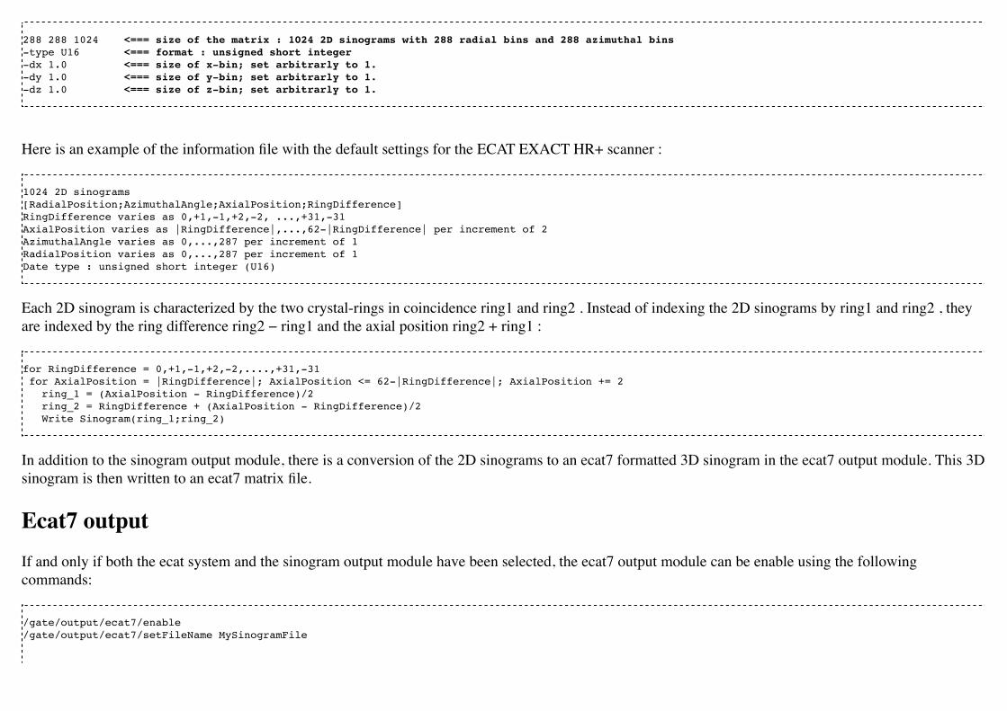
288 288 1024 <=== size of the matrix : 1024 2D sinograms with 288 radial bins and 288 azimuthal bins-type U16 <=== format : unsigned short integer-dx 1.0 <=== size of x-bin; set arbitrarly to 1.-dy 1.0 <=== size of y-bin; set arbitrarly to 1.-dz 1.0 <=== size of z-bin; set arbitrarly to 1.

Here is an example of the information file with the default settings for the ECAT EXACT HR+ scanner :

1024 2D sinograms[RadialPosition;AzimuthalAngle;AxialPosition;RingDifference]RingDifference varies as 0,+1,-1,+2,-2, ...,+31,-31AxialPosition varies as |RingDifference|,...,62-|RingDifference| per increment of 2AzimuthalAngle varies as 0,...,287 per increment of 1RadialPosition varies as 0,...,287 per increment of 1Date type : unsigned short integer (U16)

Each 2D sinogram is characterized by the two crystal-rings in coincidence ring1 and ring2 . Instead of indexing the 2D sinograms by ring1 and ring2 , theyare indexed by the ring difference ring2 − ring1 and the axial position ring2 + ring1 :

for RingDifference = 0,+1,-1,+2,-2,....,+31,-31 for AxialPosition = |RingDifference|; AxialPosition <= 62-|RingDifference|; AxialPosition += 2 ring_1 = (AxialPosition - RingDifference)/2 ring_2 = RingDifference + (AxialPosition - RingDifference)/2 Write Sinogram(ring_1;ring_2)

In addition to the sinogram output module, there is a conversion of the 2D sinograms to an ecat7 formatted 3D sinogram in the ecat7 output module. This 3Dsinogram is then written to an ecat7 matrix file.

Ecat7 outputIf and only if both the ecat system and the sinogram output module have been selected, the ecat7 output module can be enable using the followingcommands:

/gate/output/ecat7/enable/gate/output/ecat7/setFileName MySinogramFile

This module writes the content of the 2D sinograms defined in the sinogram output module to an ecat7 formatted matrix scan file, the native file format fromCPS Innovations (Knoxville (TN), U.S.A.) for their ECAT scanner family. Due to the large size of a full 3D PET data set, the data set size is reduced beforewriting it to disk. Therefore it is not possible to go back from an ecat7 formatted 3D sinogram to the original 2D sinograms set.

Installation

In order to compile the ecat7 output module of Gate, the ecat library written at the PET Unit of the Catholic University of Louvain-la-Neuve (UCL,Belgium) is required. It can be downloaded from their web site: http://www.topo.ucl.ac.be/ecat_Clib.html

Three files are required: the library file libecat.a and the two header files matrix.h and machine_indep.h.

To compile Gate with the ecat7 library without changing the env_gate.csh and GNUmakefile files, the environment variable ECAT7_HOME has to bedefined and set to the name of the home directory where the ecat7 library is installed (for example, /usr/local/ecat7). In this ecat7 home directory, twosubdirectories should be created : lib and include. The header files are put in the ${ECAT7_HOME}/include directory. For each system, a specificsubdirectory named after the G4SYSTEM environment variable value should be created in the ${ECAT7_HOME}/lib directory. The corresponding libraryfile libecat.a has to be located in this ${ECAT7_HOME}/lib/${G4SYSTEM} directory. The matrix.h file has to be modified to add the declaration of themh_update() function. The following line can be added in the "high level user functions" part of matrix.h :

int mh_update(MatrixFile*);

Data reduction

The polar coordinate of a LOR is approximately defined by the crystal-ring index difference between the 2 rings in coincidence. For a scanner with N crystalrings, the total number of polar samples is given by 2 × N − 1. Usually, on ecat systems, not all crystal-ring differences are recorded. Only absolute crystal-ring differences up to a given value, referred to as the maximum ring difference, are recorded. In Gate, this maximum ring difference is defined using:

/gate/output/ecat7/maxringdiff 22

The value of the maximum ring difference should be smaller than N.

A polar mashing is applied to group 2D sinograms with adjacent polar coordinates. The size of this grouping is called the span [reference]. Its minimumvalue is 3 and it should be an odd integer. The span value can be set using:

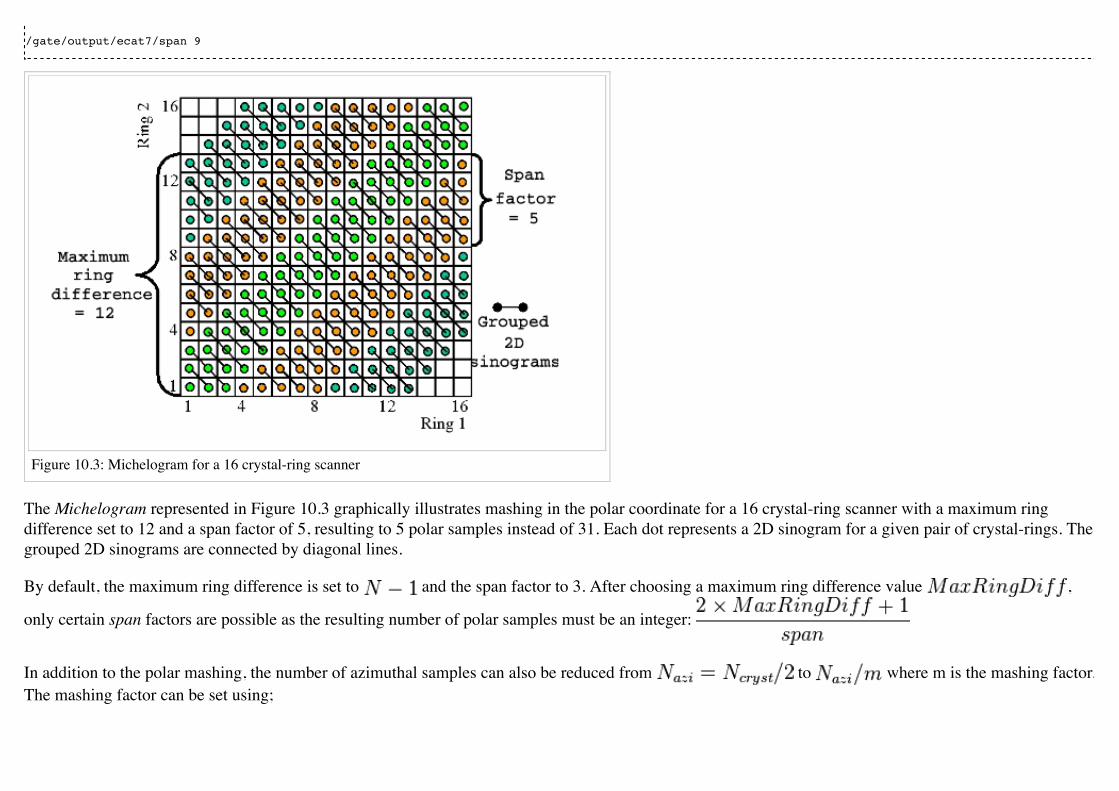
/gate/output/ecat7/span 9

Figure 10.3: Michelogram for a 16 crystal-ring scanner

The Michelogram represented in Figure 10.3 graphically illustrates mashing in the polar coordinate for a 16 crystal-ring scanner with a maximum ringdifference set to 12 and a span factor of 5, resulting to 5 polar samples instead of 31. Each dot represents a 2D sinogram for a given pair of crystal-rings. Thegrouped 2D sinograms are connected by diagonal lines.

By default, the maximum ring difference is set to and the span factor to 3. After choosing a maximum ring difference value ,

only certain span factors are possible as the resulting number of polar samples must be an integer:

In addition to the polar mashing, the number of azimuthal samples can also be reduced from to where m is the mashing factor.The mashing factor can be set using;

/gate/output/ecat7/mashing 2

The default mashing value is 1.

Sinogram file

At the end of each run, a new 3D sinogram is written with an incremental frame indexing. For example, with the following configuration, 5 frames of 60seconds each will be generated :

/gate/application/setTimeSlice 60 s/gate/application/setTimeStart 0 s/gate/appication/setTimeStop 300 s

The ECAT code of the scanner model is specified by

/gate/output/ecat7/system 962

This information can be needed by some ecat7 based reconstruction routines.

It should be noted that not all fields of the main-header or sub-header are filled. In particular, the coincidence_sampling_mode field of the main-header isalways set to Prompts and Delayed (1), regardless of the value of the /gate/output/sinogram/TruesOnly tag.

For the scan sub-header, the value of the prompts field is correctly filled and the value of the delayed field is set to the actual number of randomcoincidences, and not to the number of delayed coincidences (not simulated).

The radial bin size in the scan sub-header is set to half the value of the crystal transverse sampling and does not take into account the arc and depth-of-interaction (DOI) effects. After arc correction, the radial bin size should be slightly increased to account for the DOI effect. Note that this correction isincluded in the reconstruction software provided with theECAT scanners.

Figure 10.4: Increase of the radial bin size due to the DOI effect.

LMF outputThe Crystal Clear Collaboration has developed a List Mode Format (LMF) to store the data of ClearPET prototypes. Monte Carlo data generated by GATEcan also be stored under the same format using the class GateToLMF. This format is only available for the cylindricalPET system (see Users GuideV8.0:Defining a system) and GATE can only store single events.

Several tools enabling the reading of this format and the processing of events are implemented in the LMF library. As an example, coincidences can becreated from GATE single events. It is also possible to apply different dead-times, and even to generate sinograms in the Interfile format as used by the STIRlibrary, which implements several image reconstruction algorithms.

The LMF library and its documentation are available on the OpenGate web site.

Size of information to be stored in LMF.Information Size (bytes/single) Real machines GATE

Time 8 YES YESEnergy 1 YES YESdetector ID 2 YES YESPET's axial position 2 YES YESPET's angular position 2 YES YESrun ID 4 NO YESevent ID 4 NO YESsource ID 2 NO YESsource XYZ Position 6 NO YESglobal XYZ Position 6 NO YESnumber of Compton in phantomSD 1 NO YESnumber of Compton in crystalSD 1 NO YES

LMF data are composed of two files with the same base-name, but different extensions :

An ASCII file with a .cch extension contains general information about the scan and about the scanner, like the scan duration, the sizes of thedetectors, or the angular rotation speed.A binary file with a .ccs extension contains headers, which set the topology of the scanner, followed by fixed size records.

The user can generate these two output files automatically by using the macro scripting. All pieces of information are optional, except time, which makes theClearPET LMF quite versatile. Table 10.7.2 lists all options and memory requirements that can be stored in the LMF event record when using thecylindricalPET system :

/gate/output/lmf/enable ( or /gate/output/lmf/disable to disable LMF output (but it is disable by default)/gate/output/lmf/setFileName myLMFFile <=== to set the LMF files name. Here the output files will be myLMFFile.ccs and myLMFFile.cch/gate/output/lmf/setDetectorIDBool 1 <=== to store (1) or to not store (0) the detector ID/gate/output/lmf/setEnergyBool 1 <=== to store (1) or to not store (0) the energy /gate/output/lmf/setGantryAxialPosBool 0 <=== to store (1) or to not store (0) the axial position/gate/output/lmf/setGantryAngularPosBool 0 <=== to store (1) or to not store (0) the angular position/gate/output/lmf/setSourcePosBool 0 <===The following lines must always be included, with option set to 0

/gate/output/lmf/setNeighbourBool 0/gate/output/lmf/setNeighbourhoodOrder 0/gate/output/lmf/setCoincidenceBool 0/gate/output/lmf/setGateDigiBool 1 <===all information that is not available in real acquisitions is stored in a GateDigi record /gate/output/lmf/setComptonBool 1 <===to store (1) or to not store (0) the number of Compton scattering that occured in a phantomSD /gate/output/lmf/setComptonDetectorBool 1 <===to store (1) or to not store (0) the number of Compton scattering that occured in a crystalSD /gate/output/lmf/setSourceIDBool 0 <=== to store (1) or to not store (0) the source ID/gate/output/lmf/setSourceXYZPosBool 0 <=== to store (1) or to not store (0) the source XYZ position/gate/output/lmf/setGlobalXYZPosBool 0 <=== to store (1) or to not store (0) the real XYZ position/gate/output/lmf/setEventIDBool 1 <=== to store (1) or to not store (0) the event ID/gate/output/lmf/setRunIDBool 1 <=== to store (1) or to not store (0) the run ID

Limitations

The LMF format was originally designed for the development of small animal PET scanners for which the number of crystals is smaller than for clinicalPET scanners. Consequently, the user should carefully read the LMF specifications and make sure that this format allows him to model his scanner design. Inparticular, the maximum number of sub-volumes in a volume (e.g. the maximum number of sub-modules in a module) is set by the number of bits used toencode the sub-volume ID. The final ID encoding the position of an event has to be stored on 16, 32, or 64 bits only.

Image CT outputThe imageCT output is a binary matrix of float numbers that stores the simulated CT image and is produced for each time slice.

/gate/output/imageCT/enable/gate/output/imageCT/setFileName test

The output file name is "test_xxx.dat", where xxx is the corresponding time slice number.

In the case of the fast simulation mode, the number of pixels is set by :

/gate/output/imageCT/numPixelX 80/gate/output/imageCT/numPixelY 80

In the case of VRT simulation mode (see Users Guide V8.0:Defining a system#CTscanner), the VRT K factor is set by :

/gate/output/imageCT/vrtFactor 10

Finally the random seed can be defined using:

/gate/output/imageCT/setStartSeed 676567

Retrieved from "http://wiki.opengatecollaboration.org/index.php?title=Users_Guide_V8.0:Data_output&oldid=907"


Users Guide V8.0:Generating and tracking optical photonsFrom Wiki OpenGATE

Contents1 Introduction2 Optical Photon Generation3 Optical System4 Defining material properties

4.1 Scintillation4.2 Absorption4.3 Mie/Rayleigh Scattering4.4 Fluorescence4.5 Boundary Processes

5 Defining surfaces5.1 LUT Davis Model5.2 UNIFIED Model

6 Digitizer7 Optical Imaging Simulation Outputs

7.1 Root output7.2 Binary output of projection set

8 Example of an Optical Imaging Simulation9 Bibliography

IntroductionTo use the optical photon capabilities of GATE, the GATE_USE_OPTICAL variable has to be set to ON in the configuration process using ccmake.

Before discussing how to use the optical photon tracking, it has to be mentioned that there are a few disadvantages in using optical transport. First, thesimulation time will increase dramatically. For example, most scintillators used in PET generate in the order of 10,000 optical photons at 511 keV, whichmeans that approximately 10,000 more particles have to be tracked for each annihilation photon that is detected. Although the tracking of optical photons isrelatively fast, a simulation with optical photon tracking can easily be a factor thousand slower than one without. Finally, in order to perform opticalsimulations, many parameters are needed for the materials and surfaces, some of which may be difficult to determine.

Optical Photon Generation

/gate/source/addSource Mysource gps/gate/source/Mysource/gps/particle opticalphoton/gate/source/Mysource/gps/energytype Mono/gate/source/Mysource/gps/angtype iso

An optical photon with a wave length of 530nm corresponds to an optical photon of energy=2.34eV [approximation: 1240/E(eV) = wavelength (nm)]:

/gate/source/Mysource/gps/monoenergy 2.34 eV

An optical photon which is not assigned a polarization at production may not be Rayleigh scattered:

/gate/source/Mysource/gps/polarization 1 0 0

Optical SystemThe GATE OpticalSystem is appropriate to model Optical Imaging systems. This system is defined in the following section of the Users Guide: Users GuideV8.0:Defining_a_system#OpticalSystem.

Defining material propertiesThe optical properties of materials are stored in a material property table. In this table each of the properties of a material is identified by a name. There aretwo kinds of properties. The first are constant properties, these contain only one value. The second are property vectors, these contain properties that dependon the energy of the optical photon. Such a vector is a list of energy-value pairs.

The property tables for the materials used in a simulation are to be stored in a file separate from the material database. This makes it easier to change theproperties without having to change the material database. This file should be named Materials.xml. When Gate reads in a material from the materialsdatabase, it also checks if the Materials.xml file contains a property table for this material. If so, this table is read in and coupled to the material.

Scintillation

A scintillator is characterized by its photon emission spectrum. The scintillation follows an exponential decay with two time constants, a fast and a slow one.The relative strength of the fast component FASTCOMPONENT as a fraction of total scintillation yield is given by the YIELDRATIO. The emissionspectra of both decays are given by the property vectors FASTCOMPONENT and SLOWCOMPONENT and the time constantsFASTTIMECONSTANT and SLOWTIMECONSTANT. These vectors specify the probability that a photon with the given energy is emitted. The sum ofeach of the vectors should therefore be one.

In order to have scintillation in a material, the first parameter that has to be specified is the SCINTILLATIONYIELD (1/Mev, 1/keV), which gives thenumber of photons that is emitted per amount of energy absorbed, or, more precisely, it gives the expectation value of this number, since the real number ofemitted photons follows a normal distribution. The variance of this normal distribution is RESOLUTION-SCALE times this expectation value. Thus, forexample, when a gamma photon deposits amount of energy in the scintillator, optical photons are emitted with an expectation value of = E .SCINTILLATIONYIELD

and a standard deviation of

The parameters RESOLUTIONSCALE can be calculated from the energy resolution of the scintillator. The energy resolutions specified in the literature maycontain contributions of electronic noise. The energy resolution needed to calculate the RESOLUTIONSCALE should be the intrinsic energy resolution of thescintillator.

where is the energy resolution (FWHM - Full width at half maximum ) at energy .

<material name="LSO"> <propertiestable> <property name="SCINTILLATIONYIELD" value="26000" unit="1/MeV"/> <property name="RESOLUTIONSCALE" value="4.41"/> <property name="FASTTIMECONSTANT" value="40" unit="ns"/> <property name="YIELDRATIO" value="1"/> <propertyvector name="FASTCOMPONENT" energyunit="eV"> <ve energy="2.95167" value="1"/>

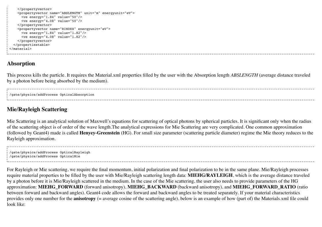
</propertyvector> <propertyvector name="ABSLENGTH" unit="m" energyunit="eV"> <ve energy="1.84" value="50"/> <ve energy="4.08" value="50"/> </propertyvector> <propertyvector name="RINDEX" energyunit="eV"> <ve energy="1.84" value="1.82"/> <ve energy="4.08" value="1.82"/> </propertyvector> </propertiestable> </material>

Absorption

This process kills the particle. It requires the Material.xml properties filled by the user with the Absorption length ABSLENGTH (average distance traveledby a photon before being absorbed by the medium).

/gate/physics/addProcess OpticalAbsorption

Mie/Rayleigh Scattering

Mie Scattering is an analytical solution of Maxwell’s equations for scattering of optical photons by spherical particles. It is significant only when the radiusof the scattering object is of order of the wave length.The analytical expressions for Mie Scattering are very complicated. One common approximation(followed by Geant4) made is called Henyey-Greenstein (HG). For small size parameter (scattering particle diameter) regime the Mie theory reduces to theRayleigh approximation.

/gate/physics/addProcess OpticalRayleigh /gate/physics/addProcess OpticalMie

For Rayleigh or Mie scattering, we require the final momentum, initial polarization and final polarization to be in the same plane. Mie/Rayleigh processesrequire material properties to be filled by the user with Mie/Rayleigh scattering length data: MIEHG/RAYLEIGH, which is the average distance traveledby a photon before it is Mie/Rayleigh scattered in the medium. In the case of the Mie scattering, the user also needs to provide parameters of the HGapproximation: MIEHG_FORWARD (forward anisotropy), MIEHG_BACKWARD (backward anisotropy), and MIEHG_FORWARD_RATIO (ratiobetween forward and backward angles). Geant4 code allows the forward and backward angles to be treated separately. If your material characteristicsprovides only one number for the anisotropy (= average cosine of the scattering angle), below is an example of how (part of) the Materials.xml file couldlook like:

<material name="Biomimic"> <propertiestable> <propertyvector name="ABSLENGTH" unit="cm" energyunit="eV"> <ve energy="1.97" value="0.926"/> <ve energy="2.34" value="0.847"/> </propertyvector> <propertyvector name="RINDEX" energyunit="eV"> <ve energy="1.97" value="1.521"/> <ve energy="2.34" value="1.521"/> </propertyvector> <property name="MIEHG_FORWARD" value="0.62" /> <property name="MIEHG_BACKWARD" value="0.62" /> <property name="MIEHG_FORWARD_RATIO" value="1.0" /> <propertyvector name="MIEHG" unit="cm" energyunit="eV"> <ve energy="1.97" value="0.04"/> <ve energy="2.34" value="0.043"/> </propertyvector> </propertiestable> </material>

Fluorescence

Fluorescence is a 3 step process: The fluorophore is in an excited state after the absorption of an optical photon provided by an external source (laser, lamp).The life time of the excited state is of order of 1-10ns during which the fluorophore interacts with its environment and ends-up in a relaxed-excited state. Thelast step is the emission of a fluorescent photon which energy/wave length is smaller(larger) than the one of the excitation optical photon.

Geant4 simulates the WaveLength Shifting (WLS) fibers that are used in High Energy Physics experiments. As an example, the CMS hadronic EndCapcalorimeter is made of scintillator tiles with WLS fibers embedded. These fibers collect/absorb blue light produced in tiles and re-emit green light so that asmuch light reaches the PMTs. A new class in Gate has been implemented as a physics builder class that inherits from the G4OpWLS class. The following

command line enables the optical photon fluorescence:

/gate/physics/addProcess OpticalWLS

Gate user needs to provide four parameters/properties to define the fluorescent material: RINDEX, WLSABSLENGTH, WLSCOMPONENT andWLSTIMECONSTANT. The WLSABSLENGTH defines the fluorescence absorption length which is the average distance travelled by a photon before itis absorbed by the fluorophore. This distance could be very small but probably not set to 0 otherwise the photon will be absorbed immediately upon enteringthe fluorescent volume and fluorescent photon will appear only from the surface. The WLSCOMPONENT describes the emission spectrum of thefluorescent volume by giving the relative strength between different photon energies. Usually these numbers are taken from measurements (i.e. emissionspectrum). The WLSTIMECONSTANT defines the time delay between the absorption and re-emission.

Simulation of the Fluorescein [see http://en.wikipedia.org/wiki/Fluorescein]

We define the refractive index of the fluorophore’s environment (water or alcohol):<material name="Fluorescein"><propertiestable><propertyvector name="RINDEX" energyunit="eV"><ve energy="1.0" value="1.4"/><ve energy="4.13" value="1.4"/></propertyvector>

The WLS process has an absorption spectrum and an emission spectrum. If these overlap then a WLS photon may in turn be absorpted and emitted again. Ifyou do not want that you need to avoid such overlap. The WLS process does not distinguish between 'original' photons and WLS photons.

We describe the fluorescein absorption length taken from measurements or literature as function of the photon energy:<propertyvector name="WLSABSLENGTH" unit="cm" energyunit="eV"><ve energy="3.19" value="2.81"/><ve energy="3.20" value="2.82"/><ve energy="3.21" value="2.81"/></propertyvector>

We describe the fluorescein Emission spectrum taken from measurements or literature as function of the photon energy:<propertyvector name="WLSCOMPONENT" energyunit="eV"><ve energy="1.771" value="0.016"/><ve energy="1.850" value="0.024"/><ve energy="1.901" value="0.040"/><ve energy="2.003" value="0.111"/><ve energy="2.073" value="0.206"/><ve energy="2.141" value="0.325"/>

<ve energy="2.171" value="0.413"/><ve energy="2.210" value="0.540"/><ve energy="2.250" value="0.683"/><ve energy="2.343" value="0.873"/><ve energy="2.384" value="0.968"/><ve energy="2.484" value="0.817"/><ve energy="2.749" value="0.008"/><ve energy="3.099" value="0.008"/></propertyvector><property name="WLSTIMECONSTANT" value="1.7" unit="ns"/></propertiestable></material>

Boundary Processes

When a photon arrives at a medium boundary its behavior depends on the nature of the two materials that join at that boundary.

/gate/physics/addProcess OpticalBoundary

In the case of two dielectric materials, the photon can undergo total internal reflection, refraction or reflection, depending on the photon’s wavelength, angleof incidence, and the refractive indices on both sides of the boundary. In the case of an interface between a dielectric and a metal, the photon can be absorbedby the metal or reflected back into the dielectric. When simulating a perfectly smooth surface, the user doesn't have to provide a G4Surface. The onlyrelevant property is the refractive index (RINDEX) of the two materials on either side of the interface. Geant4 will calculate from Snell's Law theprobabilities of refraction and reflections.

Defining surfaces

The photon travels through the surface between the two volumes Volume1 and Volume2. To create an optical surface with the name Surface-From-Volume1-To-Volume2, the following commands should be used:

/gate/Volume2/surfaces/name Surface-From-Volume1-To-Volume2/gate/Volume2/surfaces/insert Volume1

The surface between Volume1 and Volume2 is NOT the same surface as that between Volume2 and Volume1; the surface definition is directional. Whenthere is optical transport in both directions, two surfaces should be created. To load the surface properties stored in the Surfaces.xml file. Surface_name canbe any surface defined in the Surfaces.xml file:

/gate/Volume2/surfaces/Surface-From-Volume1-To-Volume2/SetSurface Surface_name

In Gate, two simulation models that are used at the boundary are available. The recently implemented LUTDavis model (GATE V8.0) and the traditionalUNIFIED model (see: source/geometry/src/GateSurface.cc).

LUT Davis Model

Please Note: Necessary modifications in Geant4 are not implemented until Summer 2017. The user can manually modify the Geant4 code. Find detailedinstructions here: Enabling LUT Davis Model

Available in GATE V8.0 is a model for optical transport called the LUT Davis model [Roncali& Cherry(2013)]. The model is based on measured surfacedata and allows the user to choose from a list of available surface finishes. Provided are a rough and a polished surface that can be used without reflector, orin combination with a specular reflector (e.g. ESR) or a Lambertian reflector (e.g. Teflon). The specular reflector can be coupled to the crystal with air oroptical grease. Teflon tape is wrapped around the crystal with 4 layers.

Surface names of available LUTs.BARE TEFLON ESR AIR ESR GREASE

POLISHED Polished_LUT PolishedTeflon_LUT PolishedESR_LUT PolishedESRGrease_LUTROUGH Rough_LUT RoughTeflon_LUT RoughESR_LUT RoughESRGrease_LUT

The user can extend the list of finishes with custom measured surface data. In GATE V8.0, this can be achieved by contacting the developers of the LUTDavis model. In future releases, a tool to calculate LUTs will be provided in form of a graphical user interface. In the LUT database, typical roughnessparameters obtained from the measurements are provided to characterize the type of surface modelled:

ROUGH Ra=0.48 µm, σ=0.57 µm, Rpv=3.12 µmPOLISHED Ra=20.8 nm, σ=26.2 nm, Rpv=34.7 nm

with Ra = average roughness; σ = rms roughness, Rpv = peak-to-valley ratio.

The desired finish should be defined in Surfaces.xml (file available in https://github.com/OpenGATE/GateContrib/tree/master/imaging/LUTDavisModel):

<surface model="DAVIS" name="RoughTeflon_LUT" type="dielectric_LUTDAVIS" finish="RoughTeflon_LUT"> </surface>

The detector surface, called Detector_LUT, defines a polished surface coupled to a photodetector with optical grease or a glass interface (similar index ofrefraction 1.5). Any surface can be used as a detector surface when the Efficiency is set according to the following example:

<surface model="DAVIS" name="Detector_LUT" type="dielectric_LUTDAVIS" finish="Detector_LUT"> <propertiestable> <propertyvector name="EFFICIENCY" energyunit="eV"> <ve energy="1.84" value="1"/> <ve energy="4.08" value="1"/> </propertyvector> </propertiestable> </surface>

Running the simulation produces an output in the terminal confirming that the LUT data is read in correctly. The user should check the presence of theselines in the terminal. For example:

===== XML PATH ====: ./Surfaces.xml ===== XML PATH ====: ...LUT DAVIS - data file: .../Rough_LUT.dat read in! Reflectivity LUT DAVIS - data file: .../Rough_LUTR.dat read in! ===== XML PATH ====: ./Surfaces.xml===== XML PATH ====: ...LUT DAVIS - data file: .../Detector_LUT.dat read in! Reflectivity LUT DAVIS - data file: .../Detector_LUTR.dat read in!

Detection of optical photons

Once the simulation is finished, the optical photon data can be found in the Hits Tree in the ROOT output. The Hits Tree consists of events that ended theirpath in the geometry defined as the sensitive detector (SD). Thus, photons can either be detected or absorbed in the crystal material when set as SD. The usercan identify the optical photons from other particles using the PDGEncoding (0 for optical photons).

Example

The example (https://github.com/OpenGATE/GateContrib/tree/master/imaging/LUTDavisModel) includes a 3 mm x 3 mm x 20 mm scintillation crystalcoupled to a 3 mm x 3 mm detector area. The source is positioned at the side of the crystal, irradiating it at 10 mm depth. The set surface isRoughTeflon_LUT in combination with the Detector_LUT as the photo detector surface.

Background

The crystal topography is obtained with atomic force microscopy (AFM). From the AFM data, the probability of reflection (1) and the reflection directions(2) are computationally determined, for incidence angles ranging from 0° to 90°. Each LUT is computed for a given surface and reflector configuration. Thereflection probability in the LUT combines two cases: directly reflected photons from the crystal surface and photons that are transmitted to the reflectorsurface and later re-enter the crystal. The key operations of the reflection process are the following: The angle between the incident photon (Old Momentum)and the surface normal are calculated. The probability of reflection is extracted from the first LUT. A Bernoulli test determines whether the photon isreflected or transmitted. In case of reflection two angles are drawn from the reflection direction LUT.

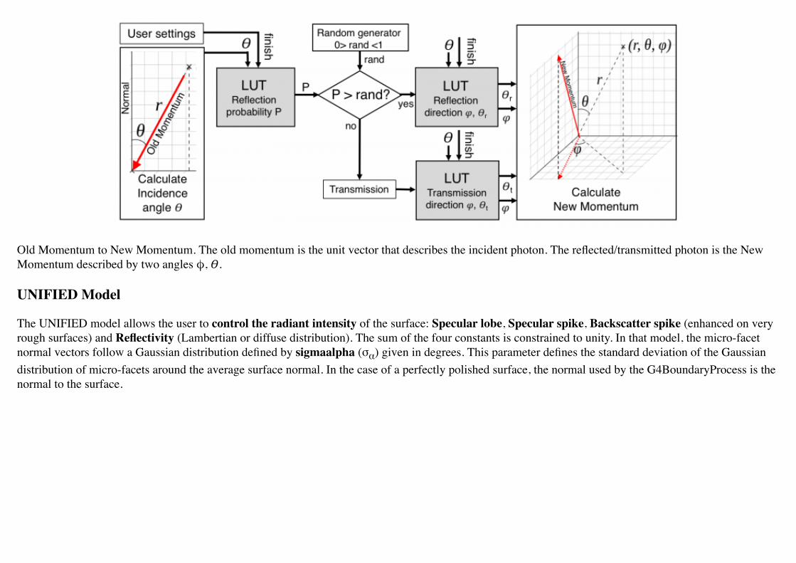
Old Momentum to New Momentum. The old momentum is the unit vector that describes the incident photon. The reflected/transmitted photon is the NewMomentum described by two angles φ, !.

UNIFIED Model

The UNIFIED model allows the user to control the radiant intensity of the surface: Specular lobe, Specular spike, Backscatter spike (enhanced on veryrough surfaces) and Reflectivity (Lambertian or diffuse distribution). The sum of the four constants is constrained to unity. In that model, the micro-facetnormal vectors follow a Gaussian distribution defined by sigmaalpha (σα) given in degrees. This parameter defines the standard deviation of the Gaussiandistribution of micro-facets around the average surface normal. In the case of a perfectly polished surface, the normal used by the G4BoundaryProcess is thenormal to the surface.

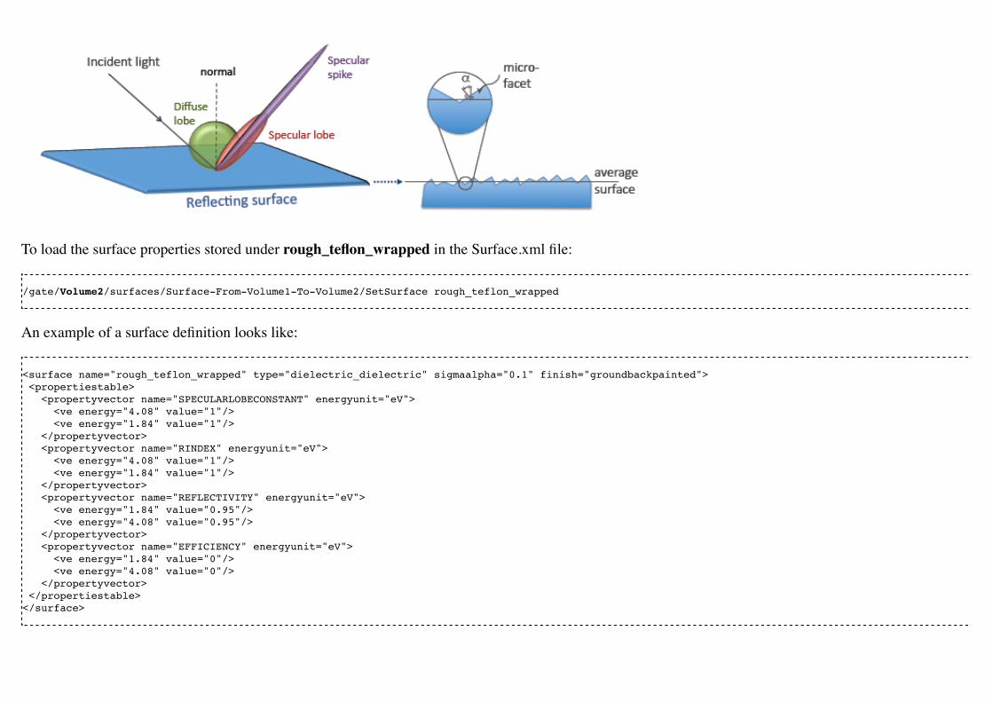
To load the surface properties stored under rough_teflon_wrapped in the Surface.xml file:

/gate/Volume2/surfaces/Surface-From-Volume1-To-Volume2/SetSurface rough_teflon_wrapped

An example of a surface definition looks like:

<surface name="rough_teflon_wrapped" type="dielectric_dielectric" sigmaalpha="0.1" finish="groundbackpainted"> <propertiestable> <propertyvector name="SPECULARLOBECONSTANT" energyunit="eV"> <ve energy="4.08" value="1"/> <ve energy="1.84" value="1"/> </propertyvector> <propertyvector name="RINDEX" energyunit="eV"> <ve energy="4.08" value="1"/> <ve energy="1.84" value="1"/> </propertyvector> <propertyvector name="REFLECTIVITY" energyunit="eV"> <ve energy="1.84" value="0.95"/> <ve energy="4.08" value="0.95"/> </propertyvector> <propertyvector name="EFFICIENCY" energyunit="eV"> <ve energy="1.84" value="0"/> <ve energy="4.08" value="0"/> </propertyvector> </propertiestable></surface>

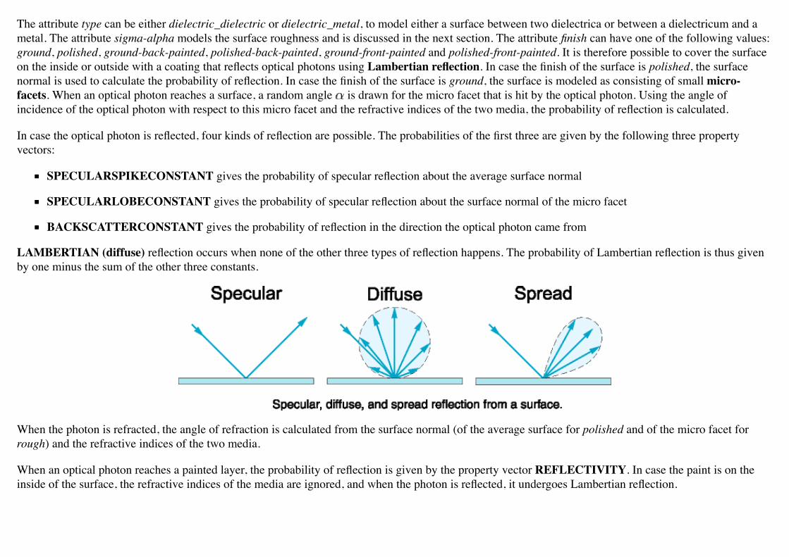
The attribute type can be either dielectric_dielectric or dielectric_metal, to model either a surface between two dielectrica or between a dielectricum and ametal. The attribute sigma-alpha models the surface roughness and is discussed in the next section. The attribute finish can have one of the following values:ground, polished, ground-back-painted, polished-back-painted, ground-front-painted and polished-front-painted. It is therefore possible to cover the surfaceon the inside or outside with a coating that reflects optical photons using Lambertian reflection. In case the finish of the surface is polished, the surfacenormal is used to calculate the probability of reflection. In case the finish of the surface is ground, the surface is modeled as consisting of small micro-facets. When an optical photon reaches a surface, a random angle is drawn for the micro facet that is hit by the optical photon. Using the angle ofincidence of the optical photon with respect to this micro facet and the refractive indices of the two media, the probability of reflection is calculated.

In case the optical photon is reflected, four kinds of reflection are possible. The probabilities of the first three are given by the following three propertyvectors:

SPECULARSPIKECONSTANT gives the probability of specular reflection about the average surface normal

SPECULARLOBECONSTANT gives the probability of specular reflection about the surface normal of the micro facet

BACKSCATTERCONSTANT gives the probability of reflection in the direction the optical photon came from

LAMBERTIAN (diffuse) reflection occurs when none of the other three types of reflection happens. The probability of Lambertian reflection is thus givenby one minus the sum of the other three constants.

When the photon is refracted, the angle of refraction is calculated from the surface normal (of the average surface for polished and of the micro facet forrough) and the refractive indices of the two media.

When an optical photon reaches a painted layer, the probability of reflection is given by the property vector REFLECTIVITY. In case the paint is on theinside of the surface, the refractive indices of the media are ignored, and when the photon is reflected, it undergoes Lambertian reflection.

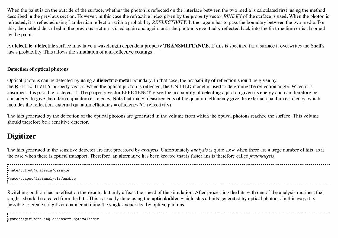
When the paint is on the outside of the surface, whether the photon is reflected on the interface between the two media is calculated first, using the methoddescribed in the previous section. However, in this case the refractive index given by the property vector RINDEX of the surface is used. When the photon isrefracted, it is reflected using Lambertian reflection with a probability REFLECTIVITY. It then again has to pass the boundary between the two media. Forthis, the method described in the previous section is used again and again, until the photon is eventually reflected back into the first medium or is absorbedby the paint.

A dielectric_dielectric surface may have a wavelength dependent property TRANSMITTANCE. If this is specified for a surface it overwrites the Snell'slaw's probability. This allows the simulation of anti-reflective coatings.

Detection of optical photons

Optical photons can be detected by using a dielectric-metal boundary. In that case, the probability of reflection should be given bythe REFLECTIVITY property vector. When the optical photon is reflected, the UNIFIED model is used to determine the reflection angle. When it isabsorbed, it is possible to detect it. The property vector EFFICIENCY gives the probability of detecting a photon given its energy and can therefore beconsidered to give the internal quantum efficiency. Note that many measurements of the quantum efficiency give the external quantum efficiency, whichincludes the reflection: external quantum efficiency = efficiency*(1-reflectivity).

The hits generated by the detection of the optical photons are generated in the volume from which the optical photons reached the surface. This volumeshould therefore be a sensitive detector.

DigitizerThe hits generated in the sensitive detector are first processed by analysis. Unfortunately analysis is quite slow when there are a large number of hits, as isthe case when there is optical transport. Therefore, an alternative has been created that is faster ans is therefore called fastanalysis.

/gate/output/analysis/disable

/gate/output/fastanalysis/enable

Switching both on has no effect on the results, but only affects the speed of the simulation. After processing the hits with one of the analysis routines, thesingles should be created from the hits. This is usually done using the opticaladder which adds all hits generated by optical photons. In this way, it ispossible to create a digitizer chain containing the singles generated by optical photons.

/gate/digitizer/Singles/insert opticaladder

/gate/digitizer/Singles/insert readout/gate/digitizer/Singles/readout/setDepth your_detector_readout_level

Digitizer modules like threshold or uphold can be used (see Users Guide V8.0:Digitizer_and_readout_parameters#Thresholder_.26_Upholder). This iscrucial when you do a fluorescence experience for example. If you want to detect only fluorescent photons you need to apply an energy cut (upholder) inorder to discard high energy photons (non-fluorescent photons have higher energy than fluorescent photons).

/gate/digitizer/Singles/insert upholder/gate/digitizer/Singles/upholder/setUphold 2.0 eV/gate/digitizer/Singles/insert thresholder/gate/digitizer/Singles/thresholder/setThreshold 1.0 eV

The projection (see Projection set) associated to this digitizer records only photons corresponding to the defined energy window. The projection image istherefore the fluorescence image.

Optical Imaging Simulation Outputs

Root output

When working with optical photons, an additional ROOT tree is created: OpticalData. You can decide to fill this tree or not by using the followingcommand:

/gate/output/root/setRootOpticalFlag 0 or 1

OpticalData tree is generated with the following information:

CrystalLastHitEnergy CrystalLastHitPos_X CrystalLastHitPos_Y CrystalLastHitPos_ZEnergy and Positions of the photon last hit in the Crystal (Detected photon position)

PhantomLastHitEnergy PhantomLastHitPos_X PhantomLastHitPos_Y PhantomLastHitPos_ZEnergy and Positions of the photon last hit in the Phantom

NumCrystalWLS Number of Fluorescence processes per event(photon) in the Crystal

NumPhantomWLS Number of Fluorescence processes per event(photon) in the Phantom

NumScintillationNumber of Scintillation processes per event(photon) in the Crystal

CrystalProcessName PhantomProcessNameList of process names that occured in the Crystal or in the Phantom

MomentumDirectionx MomentumDirectiony MomentumDirectionzOptical photon momentum direction

Binary output of projection set

In order to create a projection set (see Interfile output of projection set) using the Optical System in GATE, the following lines have to be added to themacro:

/gate/output/projection/enable/gate/output/projection/setFileName your_name/gate/output/projection/projectionPlane XY/gate/output/projection/pixelSizeX 0.105 cm/gate/output/projection/pixelSizeY 0.105 cm/gate/output/projection/pixelNumberX 100/gate/output/projection/pixelNumberY 100

The result of projection set is saved in a binary file (.bin). A header file (.hdr) is also provided with the following information:

!INTERFILE := !imaging modality := optical imaging ; !GENERAL DATA := data description := GATE simulation

!name of data file := ./OpticalSimulationProjection.bin ; !GENERAL IMAGE DATA := !type of data := OPTICAL !total number of images := 1 ; !OPTICAL STUDY (general) := number of detector heads := 1 ; !number of images divided by number of energy window := 1 projection matrix size [1] := 100 projection matrix size [2] := 100 projection pixel size along X-axis (cm) [1] := 0.105 projection pixel size along Y-axis (cm) [2] := 0.105 !number of projections := 1 !extent of rotation := 360 !time per projection (sec) := 1 ; ;GATE GEOMETRY := ;Optical System x dimension (cm) := 10.5 ;Optical System y dimension (cm) := 10.5 ;Optical System z dimension (cm) := 2 ;Optical System material := Air ;Optical System x translation (cm) := 0 ;Optical System y translation (cm) := 0 ;Optical System z translation (cm) := 0 ; ;Optical System LEVEL 1 element is crystal := ;Optical System crystal x dimension (cm) := 10.5 ;Optical System crystal y dimension (cm) := 10.5 ;Optical System crystal z dimension (cm) := 1 ;Optical System crystal material := Air ; ;Optical System LEVEL 2 element is pixel := ;Optical System pixel x dimension (cm) := 2 ;Optical System pixel y dimension (cm) := 2 ;Optical System pixel z dimension (cm) := 1 ;Optical System pixel material := Air ; !END OF INTERFILE :=

Example of an Optical Imaging Simulation

In the GateContrib repository you will find simple examples of a bioluminescence/fluorescence experiment. All macros are located under imaging/Optical.In addition, a ROOT macro [DrawBranches.C] is available and draws all branches of the OpticalData tree into a postscript file.

The optical imaging system is composed of an array of pixels, an electronic board and an angular aperture that limits the range of angles over which theoptical system can accept light. The phantom is composed of a box of water and two layers made of either water, hypodermis or epidermis. In case of abioluminescence experiment, the tumor is described as a voxelized source of optical photons and is positioned under the inner layer of the phantom. In caseof a fluorescence experiment, we assigned the Rhodamine B fluorophore to each voxel of a voxelized tumor and positioned it under the inner layer of thephantom. The fluorophore is excited by two external beam light sources emitting optical photons towards the tumor.

These two experiments are available in imaging/Optical through the following macros: bioluminescence.mac and fluorescence.mac. The voxelized source orphantom is available in imaging/Optical/voxelized-source-phantom with an attenuation file and an optical-flux file. These macros will generate a root outputfile with the OpticalData tree enabled and a binary file which corresponds to the GATE ProjectionSet on the XY plane (i.e detection plane). Using the rootmacros MakeBioluminescencePlots.C and MakeFluorescencePlots.C, you can read the root output file and draw the bioluminescent/fluorescent light that isdetected by the optical system. In case of the fluorescence experiment, two plots are drawn: all detected light (any wavelength) and the fluorescent light(wavelength cut). The projection binary file (.bin and .hdr) can be viewed directly using Anatomist or Imagej. In case of the fluorescence experiment, anUpholder (uphold cut) was applied through the digitizer so the binary image illustrates the fluorescent light.

The Materials.xml file is updated with several tissues properties at specific wavelengths (from literature): brain, kidney, epidermis and hypodermis but alsowith the emission spectra of the Fluorescein and Rhodamine B.

Bibliography

The NIST XCOM (NIST-XCOM (http://www.nist.gov/pml/data/xcom/index.cfm)): Photon Cross Sections Database gives attenuation coefficients.The Database Search Form is available directly through this link Database Search Form(http://physics.nist.gov/PhysRefData/Xcom/html/xcom1.html).

A Review of the Optical Properties of Biological Tissues, IEEE J. Quantum Electronics, 26, 2166-2185 (1990) (W. F. Cheong, S. A. Prahl, and A. J.Welch). Updated by Wai-Fung Cheong. Further additions by Lihong Wang and Steven L. Jacques. August 6, 1993(http://ieeexplore.ieee.org/xpls/abs_all.jsp?arnumber=64354) - IEEE Journal of Quantum Electronics, Vol. 26, Issue 12, pp. 2166 - 2185

Optical Absorption of Water (http://omlc.ogi.edu/spectra/water/index.html) with all currently available data (presented in terms of wavelength andabsorption coefficient) - Scott Prahl, Oregon Medical Laser Center.

Optical Brain Imaging in Vivo: Techniques and Applications from Animal to Man. (E. M. C. Hillman)(http://www.ncbi.nlm.nih.gov/pubmed/17994863) - J. Biomed. Opt. 2007 Sep-Oct;12(5):051402

Refractive Index Measurement of Acute Rat Brain Tissue Slices using Optical Coherence Tomography (J. Sun, S. J. Lee, L. Wu, M. Sarntinoranontand H. Xie) (http://www.opticsinfobase.org/oe/abstract.cfm?uri=oe-20-2-1084) - Optics Express, Vol. 20, Issue 2, pp. 1084-1095 (2012)

In Vivo Optical Reflectance Imaging of Spreading Depression Waves in Rat Brain with and without Focal Cerebral Ischemia (S. Chen, Z. Feng, P. Li,S. L. Jacques, S. Zeng and Q. Luo) (http://www.ncbi.nlm.nih.gov/pubmed/16822052) - J. Biomed. Opt. 2006 May-Jun;11(3):34002

Brain Refractive Index Measured in Vivo with High-NA Defocus-Corrected Full-Field OCT and Consequences for Two-Photon Microscopy (J.Binding, J. Ben Arous, J-F. Leger, S. Gigan, C. Boccara and L. Bourdieu) (http://www.opticsinfobase.org/oe/abstract.cfm?uri=oe-19-6-4833) - OpticsExpress, Vol. 19, Issue 6, pp. 4833-4847 (2011)

Contribution of the Mitochondrial Compartment to the Optical Properties of the Rat Liver: a Theoretical and Practical Approach (B. Beauvoit, T.Kitai and B. Chance) (http://www.ncbi.nlm.nih.gov/pubmed/7696489) - Biophys. J. 1994 Dec;67(6):2501-10

Optical Properties of Native and Coagulated human Liver Tissue and Liver Metastases in the Near Infrared Range (C. T. Germer, A. Roggan, J. P.Ritz, C. Isbert, D. Albrecht, G. Muller and H. J. Buhr) (http://www.ncbi.nlm.nih.gov/pubmed/9829430) - Lasers Surg. Med. 1998;23(4):194-203

In Vivo Determination of the Optical Properties of Muscle with Time-Resolved Reflectance using a Layered Model (A. Kienle and T. Glanzmann)(http://www.ncbi.nlm.nih.gov/pubmed/10588278) - Phys. Med. Biol. 1999 Nov;44(11):2689-702

Optical Properties of Skin, Subcutaneous and Muscle Tissues: a Review (A. N. Bashkatov, E. A. Genina and V. V. Tuchin)(http://www.worldscientific.com/doi/abs/10.1142/S1793545811001319) - J. Innov. Opt. Health Sci. 04, 9 (2011)

Determination of the Optical Properties of Rat (Heart) Tissue (A. Singh1, A. E. Karsten, R. M. Smith and G. van Niekerk)(http://researchspace.csir.co.za/dspace/handle/10204/4039) - 2010 European Cells & Materials Ltd

In Vitro Double-Integrating-Sphere Optical Properties of Tissues between 630 and 1064nm (J. F. Beek†, P. Blokland, P. Posthumus, M. Aalders, J. W.Pickering, H. J. C. M. Sterenborg and M. J. C. van Gemert) (http://www.ncbi.nlm.nih.gov/pubmed/9394410) - Phys. Med. Biol. 42 (11) 1997 2255-61

Simpson R, Kohl M, Essenpreis M and Cope M 1998 Near-Infrared optical properties of ex vivo human skin and subcutaneous tissues measuredusing the Monte Carlo inversion technique Phys. Med. Biol. 43 2465-2478

Baran T M, Wilson J D, Mitra S, Yao J L, Messing E M, Waldman D L and Foster T H 2012 Optical property measurements establish the feasibility ofphotodynamic therapy as a minimally invasive intervention for tumors of the kidney J. Biomed. Opt. 17 (9) 098002

Rolfe P 2000 Brain - In vivo near-infrared spectroscopy Annu. Rev. Biomed. Eng. 2 715-754

Roncali E & Cherry S 2013 - Simulation of light transport in scintillators based on 3D characterization of crystal surfaces.(https://www.ncbi.nlm.nih.gov/pubmed/23475145) Phys. Med. Biol., Volume 58(7), p. 2185–2198.

Retrieved from "http://wiki.opengatecollaboration.org/index.php?title=Users_Guide_V8.0:Generating_and_tracking_optical_photons&oldid=934"


Users Guide V8.0:Radiotherapy General ConceptFrom Wiki OpenGATE

Contents1 General concept2 Insert a CT image in the therapy simulation

2.1 Step1: convert Dicom image to Analyze image file format2.2 Step2: define HU to materials conversion2.3 Step3: insert image as a volume

3 Dose distribution (Dosimetry)

General conceptThe Radiotherapy and Dosimetry reference paper GATE V6: a major enhancement of the GATE simulation platform enabling modelling of CT andradiotherapy is available (here) (http://www.opengatecollaboration.org/sites/default/files/Jan2011.pdf).

A list of radionuclides is availabe at NUCLEIDE.ORG (http://www.nucleide.org/DDEP_WG/DDEPdata.htm).

The concept of Actors is very important for the simulation of radiotherapy treatments and dosimetry. Actors(http://wiki.opengatecollaboration.org/index.php/Users_Guide_V8.0:Tools_to_Interact_with_the_Simulation_:_Actors) and Filters(http://wiki.opengatecollaboration.org/index.php/Users_Guide_V8.0:Tools_to_Interact_with_the_Simulation_:_Actors#Filters) are tools which allow tointeract with the simulation. They can collect information during the simulation, such as energy deposit, number of particles created in a given volume, etc.They can also modify the behavior of the simulation. There are different types of actors which collect different types of information, however somecommands and behavior are common to all actors. To use selection criteria, it is possible to add filters.

Insert a CT image in the therapy simulationFor a realistic radiotherapy simulation, one wants to use a patient CT image as the voxelized phantom. For that, the following steps must be followed.

Step1: convert Dicom image to Analyze image file format

The VV, the 4D Slicer (https://www.creatis.insa-lyon.fr/rio/vv) software can be used for this purpose. It opens the DICOM image and saves it as a headerplus raw data. It can also resample the image.

Step2: define HU to materials conversion

The following macro can be used to generate Hounsfield Unit (HU) to material conversion.

/gate/HounsfieldMaterialGenerator/SetMaterialTable MaterialsTable.txt/gate/HounsfieldMaterialGenerator/SetDensityTable DensitiesTable.txt/gate/HounsfieldMaterialGenerator/SetDensityTolerance 0.1 g/cm3/gate/HounsfieldMaterialGenerator/SetOutputMaterialDatabaseFilename myimage-HUmaterials.db/gate/HounsfieldMaterialGenerator/SetOutputHUMaterialFilename myimage-HUmat.txt/gate/HounsfieldMaterialGenerator/Generate

Step3: insert image as a volume

/gate/world/daughters/name patient/gate/world/daughters/insert ImageNestedParametrisedVolume/gate/patient/geometry/SetImage myimage.hdr/gate/geometry/setMaterialDatabase myimage-HUmaterials.db/gate/patient/geometry/SetHUToMaterialFile myimage-HUmat.txt/gate/patient/placement/setTranslation 0 0 0 mm

Dose distribution (Dosimetry)GATE allows to simulate the dose distribution in a phantom during radiotherapy (therapy with photons) and hadrontherapy (therapy with hadrons : proton,Carbon...). It also allows to perform other radiation simulations such as brachytherapy, dose deposited during x-ray imaging... Figure 1 shows an example ofa dose distribution map obtained after radiotherapy treatment on a phantom.

Figure 1: Dose distribution after radiotherapy treatment on a phantom.

The DoseActor(http://wiki.opengatecollaboration.org/index.php/Users_Guide_V7.2:Readout_parameters_for_Radiotherapy_applications:_Actors#Dose_measurement) isthe tool that is used to store the deposited dose in a 3D matrix which size and resolution can be specified. It can also be used for 1D and 2D dose maps. Itcan store dose, edep or number of hits and computes associated statistical uncertainty. The DoseActor is attached to a volume which can be voxelized or not.

Retrieved from "http://wiki.opengatecollaboration.org/index.php?title=Users_Guide_V8.0:Radiotherapy_General_Concept&oldid=690"

This page was last modified on 21 September 2016, at 09:42.

Users Guide V8.0:Nanoparticle mediated hyperthermiaFrom Wiki OpenGATE

Contents1 Pre-requisite2 Theory

2.1 Optical photon deposited energy map2.2 Pennes bioheat model and the analytical solution2.3 Hybrid Monte-Carlo and analytical simulation : a dynamic process

3 Illustration of the heat diffusion 3D map obtained by the ThermalActor4 Command lines

Pre-requisiteTo use the nanoparticle mediated hyperthermia capabilities of GATE, you have to install ITK and turn the CMake flag GATE_USE_ITK to ON in theconfiguration process using ccmake. Please find detailed instructions here: Compilation_Instructions_V8.0

TheoryOptical photon deposited energy map

The optical photons emitted by an illumination light (i.e. laser) will be absorbed by the tissues (OpticalAbsorption process) or/and by a tissue loaded with acertain concentration of nanoparticles (NanoAbsorption process).

In GATE, the optical photon is transported following a step length which is randomly sampled using the mean free path of each physics process associated tothe optical photon. The mean free path of the optical photon interaction with the nanoparticle-infused medium is . The inverse of the absorption length isreferred to as the absorption coefficient ( ) and is a function of the density of nanoparticles in the medium (N in m-3) and the nanoparticle absorption

cross-section area ( in m2) : .

Pennes bioheat model and the analytical solution

The mathematical model that describes the thermal behavior in biological perfused tissues is the Pennes bioheat model :

where represents the energy deposition by any external heat source such as the metabolic heat production in the tissue and is considered to be 0.

The first term of the equation describes the transfer of energy between objects in contact (i.e. conduction); the second term accounts for the effects of bloodperfusion in tissues. and are the biological tissue thermal conductivity, density and specific heat. Values for blood are given by and ; is thetissue blood perfusion rate which represents the volume of fluid (i.e. blood) that passes per unit time and per tissue volume. is the temperature of blood inthe main arteries and is the local tissue temperature. Pennes equation is solved analytically via Fourier transformations and convolutiontheorem. The analytical solution to the Pennes bioheat equation is

with the tissue thermal diffusivity.

The solution of the diffusion equation is equivalent to convolving the initial conditions (3D energy map) with a Gaussian with a standard deviation . The blood perfusion term appears as an exponential function. The implementation of the heat diffusion in GATE is performed using the

Insight Segmentation and Registration Toolkit (ITK) which is an open-source, cross-platform system that provides developers with an extensive suite oftools for image analysis.

Hybrid Monte-Carlo and analytical simulation : a dynamic process

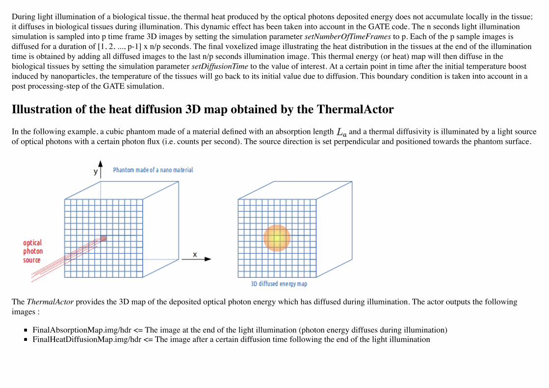
During light illumination of a biological tissue, the thermal heat produced by the optical photons deposited energy does not accumulate locally in the tissue;it diffuses in biological tissues during illumination. This dynamic effect has been taken into account in the GATE code. The n seconds light illuminationsimulation is sampled into p time frame 3D images by setting the simulation parameter setNumberOfTimeFrames to p. Each of the p sample images isdiffused for a duration of [1, 2, ..., p-1] x n/p seconds. The final voxelized image illustrating the heat distribution in the tissues at the end of the illuminationtime is obtained by adding all diffused images to the last n/p seconds illumination image. This thermal energy (or heat) map will then diffuse in thebiological tissues by setting the simulation parameter setDiffusionTime to the value of interest. At a certain point in time after the initial temperature boostinduced by nanoparticles, the temperature of the tissues will go back to its initial value due to diffusion. This boundary condition is taken into account in apost processing-step of the GATE simulation.

Illustration of the heat diffusion 3D map obtained by the ThermalActorIn the following example, a cubic phantom made of a material defined with an absorption length and a thermal diffusivity is illuminated by a light sourceof optical photons with a certain photon flux (i.e. counts per second). The source direction is set perpendicular and positioned towards the phantom surface.

The ThermalActor provides the 3D map of the deposited optical photon energy which has diffused during illumination. The actor outputs the followingimages :

FinalAbsorptionMap.img/hdr <= The image at the end of the light illumination (photon energy diffuses during illumination)FinalHeatDiffusionMap.img/hdr <= The image after a certain diffusion time following the end of the light illumination

Command lines

/gate/actor/addActor ThermalActor MyActor/gate/actor/MyActor/save 3DMap.hdr/gate/actor/MyActor/attachTo phantom/gate/actor/MyActor/stepHitType random/gate/actor/MyActor/setPosition 0. 0. 0. cm/gate/actor/MyActor/setVoxelSize 0.5 0.5 0.5 mm

Tissue thermal property : /gate/actor/MyActor/setThermalDiffusivity 0.32 mm2/s

Density and heat capacity should just be in the same unit for both blood and tissue. In the following example, the density is in kg/mm3 and the heat capacity in mJ kg/gate/actor/MyActor/setBloodDensity 1.06E-6/gate/actor/MyActor/setBloodHeatCapacity 3.6E6/gate/actor/MyActor/setTissueDensity 1.04E-6/gate/actor/MyActor/setTissueHeatCapacity 3.65E6/gate/actor/MyActor/setBloodPerfusionRate 0.004

/gate/actor/MyActor/setDiffusionTime 5 s/gate/actor/MyActor/setNumberOfTimeFrames 5

Retrieved from "http://wiki.opengatecollaboration.org/index.php?title=Users_Guide_V8.0:Nanoparticle_mediated_hyperthermia&oldid=993"


Users Guide V8.0:How to use Gate on a ClusterFrom Wiki OpenGATE

To reduce the overall computing time of GATE experiments, a parallel computing platform for running simulations in a cluster of computers was developedwhich significantly shortens the setup time and provides fast data output handling. To use Gate in cluster mode you need 3 components:

The job splitter (gjs)The file merger (gjm)A cluster aware version of Gate

Contents1 Installation of the job splitter (gjs)2 Installation of the file merger (gjm)3 Preparing your macro4 Using the job splitter5 Using the file merger6 Alternative to the file merger7 What about errors?

Installation of the job splitter (gjs)The job splitter can be installed in the same directory as Gate. Two environment variables are already added to the environment file used to compile Gate(but you can customize them):

export GC_DOT_GATE_DIR=/somedir/ export GC_GATE_EXE_DIR=/somedir/bin/Linux-g++/

The first variable indicates the location of a hidden directory called .Gate. The directory will contain the split macros for each part of the simulation. Evenwhen splitting the same macro several times, a new directory will be created for each instance (with an incremental number). In normal circumstances, onedoes not need to look into it. In case of an error, it can be used to run only a specific part of a simulation again (See #What about errors?). The secondenvironment variable indicates the location of the job splitter executable. As the Gate environment file will be used to compile the job splitter source code,the executable will likely be located in the same directory as the Gate executable.

To install, load the Gate/Geant4 environment variables, go to the job splitter directory (bash example):

source env_gate.shcd jobsplittermake

By default, the executable will be created in the jobsplitter directory. If the GATEHOME variable is correctly defined, the executable will also be copied inthe same directory as the Gate executable (same for the dynamic library).

Installation of the file merger (gjm)To install, it is the same way, go to the file merger directory and compile (bash example):

cd filemergermake

The file merger executable is located in the current directory (and will also be copied in the Gate bin directory as for the gjs program).

Preparing your macroThe cluster software should be able to handle all GATE macros. However, only ROOT is currently supported as an output format for the gjm program. So beaware that other output formats cannot yet be merged with the gjm program and you will have to do this on your own (but it is usually quite simple ~addition or mean most of the time).

If an isotope with a shorter half life than the acquisition time is simulated, then it may be useful to specify the half life in your macro as follows:

/gate/cluster/setTimeSplitHalflife 6600. s

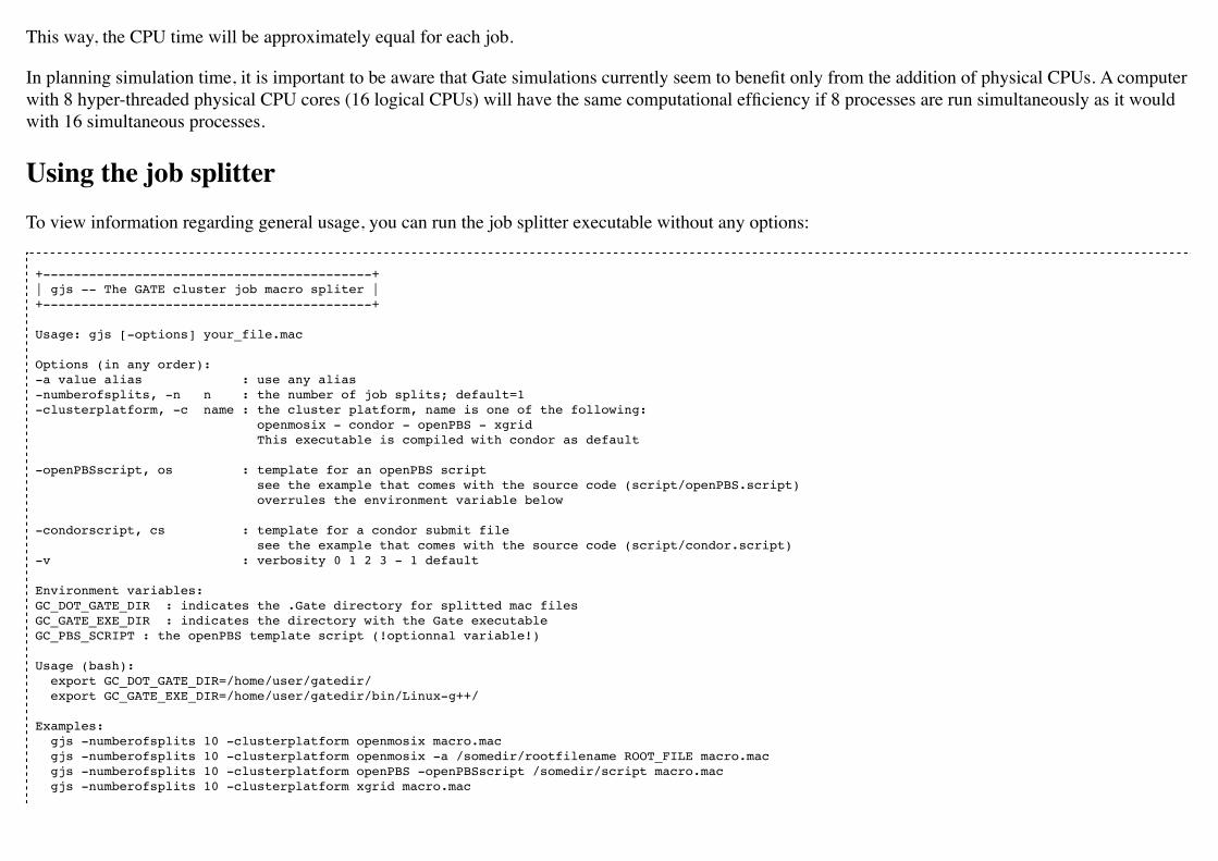
This way, the CPU time will be approximately equal for each job.

In planning simulation time, it is important to be aware that Gate simulations currently seem to benefit only from the addition of physical CPUs. A computerwith 8 hyper-threaded physical CPU cores (16 logical CPUs) will have the same computational efficiency if 8 processes are run simultaneously as it wouldwith 16 simultaneous processes.

Using the job splitterTo view information regarding general usage, you can run the job splitter executable without any options:

+-------------------------------------------+ | gjs -- The GATE cluster job macro spliter | +-------------------------------------------+

Usage: gjs [-options] your_file.mac

Options (in any order): -a value alias : use any alias -numberofsplits, -n n : the number of job splits; default=1 -clusterplatform, -c name : the cluster platform, name is one of the following: openmosix - condor - openPBS - xgrid This executable is compiled with condor as default

-openPBSscript, os : template for an openPBS script see the example that comes with the source code (script/openPBS.script) overrules the environment variable below

-condorscript, cs : template for a condor submit file see the example that comes with the source code (script/condor.script) -v : verbosity 0 1 2 3 - 1 default

Environment variables: GC_DOT_GATE_DIR : indicates the .Gate directory for splitted mac files GC_GATE_EXE_DIR : indicates the directory with the Gate executable GC_PBS_SCRIPT : the openPBS template script (!optionnal variable!)

Usage (bash): export GC_DOT_GATE_DIR=/home/user/gatedir/ export GC_GATE_EXE_DIR=/home/user/gatedir/bin/Linux-g++/

Examples: gjs -numberofsplits 10 -clusterplatform openmosix macro.mac gjs -numberofsplits 10 -clusterplatform openmosix -a /somedir/rootfilename ROOT_FILE macro.mac gjs -numberofsplits 10 -clusterplatform openPBS -openPBSscript /somedir/script macro.mac gjs -numberofsplits 10 -clusterplatform xgrid macro.mac

gjs -numberofsplits 10 /somedir/script macro.mac

The supported platforms are currently: openMosix, openPBS, Condor and Xgrid.

Let's take openMosix as an example:

gjs -numberofsplits 5 -clusterplatform openmosix macro.mac

The job splitter will subdivide the simulation macro into fully resolved, non-parameterized macros. In this case there are 5 such macros. They are located inthe .Gate directory, as specified by the GC_DOT_GATE_DIR environment variable.

A list of all the data output options is given after successful completion, as well as a list of all activated actors. The user is asked to clearly enable eachneeded output module and to give them an output file name. It is the same for actors. Remember that by default, no output module nor actor is enabled.

If an alias was expected for output files and it was not supplied, then this will be mentioned in the output options list. A standard name will be suppliedautomatically, as well as appropriate numbering.

The time of each sub-macro is manage using a virtual timeStart and a virtual timeStop calculated by the gjs and used by the command/gate/application/startDAQCluster. All defined runs and geometry updates will be totally respected. The only inconsistency in the use of gjs is when usingthe projection output: the virtualStop minus virtualStart time have to be a multiple of timeSlice, otherwise the GateToProjectionSet output will lead to anerror.

The .Gate directory will have a subdirectory called as the macro name, that contains the following files:

macro1.mac macro2.mac macro3.mac macro4.mac macro5.mac macro.split

The 5 macros are listed as well as well as the .split file that contains information about the splitted simulation and that will be used to merge the data after thesimulation (using the gjm program). The current directory, from which the jobsplitter was called, now contains the cluster submit file. In order to run thesplit simulation on the cluster, one only needs to execute or call this file with a certain program (depending on the cluster platform used).

The .Gate directory supports automatic numbering. If the same macro is used repeatedly, then the subsequent directories will be numbered using anincremental number.

Using the file mergerThe file merger have to be run giving the split file as input. To view information on general usage, just run the file merger executable without any options:

+-------------------------------------------+ | gjm -- The GATE cluster job output merger | +-------------------------------------------+

Usage: gjm [-options] your_file.split

You may give the name of the split file created by gjs (see inside the .Gate directory). !! This merger is only designed to ROOT output. !!

Options: -outDir path : where to save the output files default is PWD -v : verbosity 0 1 2 3 - 1 default -f : forced output - an existing output file will be overwritten -cleanonly : do only a the cleanup step i.e. no merging erase work directory in .Gate and the files from the parallel jobs -cleanonlyTest : just tells you what will be erased by the -cleanonly -clean : merge and then do the cleanup automatically -fastMerge : correct the output in each file, to be used with a TChain (only for Root output)

Environment variable: GC_DOT_GATE_DIR : points to the .Gate directory

To merge the output files into a single file, just supply the split file to the file merger. The output file could be used as a usual single CPU output file.

gjm macro.split

Combining: ./rootf1.root ./rootf2.root ./rootf3.root ./rootf4.root ./rootf5.root $->$ ./rootf.root

In case a single output file is not required, it is possible to use the option fastMerge. This way, the eventIDs in the ouput files are corrected locally. Figure13.1 shows the newly created tree in each ROOT file.

Figure 13.1: Example of ROOT file with added cluster eventIDs

A ROOT chain, which is a list of files containing the same tree, is then required to link the output files together for analysis. A chain for the Singles could bemade as follows (in a file called chain.c):

\{ gROOT->Reset(); TChain chain("Singles"); chain.Add("rootf1.root"); chain.Add("rootf2.root"); chain.Add("rootf3.root"); chain.Add("rootf4.root"); chain.Add("rootf5.root"); \}

Once all files are added to the chain, one can use the chain as a regular Ttree, and the normal ROOT prompt is returned:

$root chain.c

FreeType Engine v2.1.3 used to render TrueType fonts. Compiled for linux with thread support. CINT/ROOT C/C++ Interpreter version 5.15.94, June 30 2003 Type ? for help. Commands must be C++ statements. Enclose multiple statements between \{ \}. root [0] Processing chain.c... root [1] root [1] Singles->Draw("energy")

Alternative to the file mergerRoot files can also be merged by using the hadd utility on the command line:

hadd result.root file1.root file2.root ... filen.root

What about errors?If something went wrong during a simulation and a ROOT file is corrupted or incomplete, then this will be detected by the file merger. There are twooptions. First, one can restart only the specific part of the simulation that went wrong. This can be easily done, as the ROOT files are numbered and one canedit the submit file so it only launches that specific part. Alternatively, one can find the macro file that was used to start that part of the simulation in the

.Gate directory and start the simulation directly with the macro file and its corresponding seed file. The second option is to edit the split file, located in the

.Gate directory. Once the reference to the corrupted root file is removed from it, it is possible to merge the files again. At this point, the eventIDs will not bevalid anymore.

Retrieved from "http://wiki.opengatecollaboration.org/index.php?title=Users_Guide_V8.0:How_to_use_Gate_on_a_Cluster&oldid=269"


Users Guide V8.0:How to use Gate on a GPUFrom Wiki OpenGATE

Contents1 Installation of CUDA tools2 PET applications3 CT applications4 Optical applications

Installation of CUDA toolsIMPORTANT NOTE:

!! GPU modules can be used ONLY with NVIDIA hardware and CUDA tools !!

For details, see the link on the wiki installation guide page:http://wiki.opengatecollaboration.org/index.php/New_Compilation_ProcedureV7.0#GPU_.26_CUDA_tools

PET applicationsFor PET applications, the GPU manages the particle tracking within the voxelized phantom and this is why the source type is defined as a [GPUEmisTomo].Examples are provided within the GATE source package and users can find a complete example about How To define and run a complete PET simulationset-up by using a GPU architecture.

IMPORTANT NOTES:

1/ By using the GPU, phantom scatter informations are NOT available in the output files

2/ The sources radiactive decay time is NOT available with the GPU

#==================================================# VOXELIZED SOURCES#==================================================/gate/source/addSource srcvoxel GPUEmisTomo/gate/source/srcvoxel/attachPhantomTo ncat/gate/source/srcvoxel/setGPUBufferSize 1000000/gate/source/srcvoxel/setGPUDeviceID 1# Read the phantom as usual/gate/source/srcvoxel/reader/insert interfile/gate/source/srcvoxel/interfileReader/translator/insert range/gate/source/srcvoxel/interfileReader/rangeTranslator/readTable data/activities.dat/gate/source/srcvoxel/interfileReader/rangeTranslator/describe 1/gate/source/srcvoxel/interfileReader/verbose 0/gate/source/srcvoxel/interfileReader/readFile data/thorax_phantom.hdr/gate/source/srcvoxel/setType backtoback/gate/source/srcvoxel/gps/particle gamma/gate/source/srcvoxel/gps/energytype Mono/gate/source/srcvoxel/gps/monoenergy 0.511 MeV/gate/source/srcvoxel/setPosition 0 0 0 cm/gate/source/srcvoxel/gps/confine NULL/gate/source/srcvoxel/gps/angtype iso

CT applicationsFor CT applications, the GPU tracking is defined as an Actor.

Examples are provided within the GATE source package and users can find a complete example about How To define and run a complete CT simulation set-up by using a GPU architecture.

IMPORTANT NOTE:

The scannerCT system, the digitizer and the CT deticated output are NOT available with the GPU CT module. The CT detector must be define by using anactor as it is shown in the complete example provided with the source.

#==================================================# GPU Tracking#==================================================/gate/actor/addActor GPUTransTomoActor gpuactor/gate/actor/gpuactor/attachTo patient/gate/actor/gpuactor/setGPUDeviceID 1

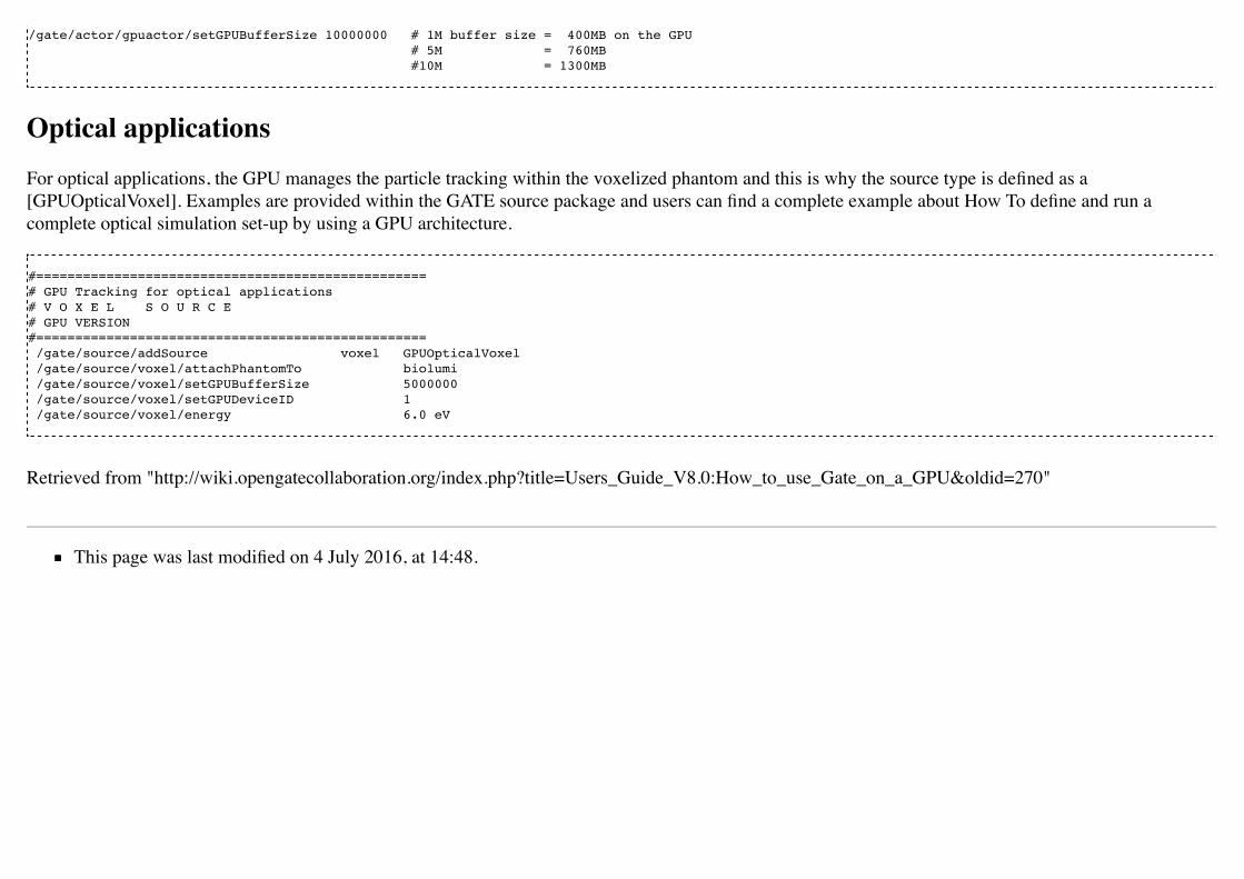
/gate/actor/gpuactor/setGPUBufferSize 10000000 # 1M buffer size = 400MB on the GPU # 5M = 760MB #10M = 1300MB

Optical applicationsFor optical applications, the GPU manages the particle tracking within the voxelized phantom and this is why the source type is defined as a[GPUOpticalVoxel]. Examples are provided within the GATE source package and users can find a complete example about How To define and run acomplete optical simulation set-up by using a GPU architecture.

#==================================================# GPU Tracking for optical applications# V O X E L S O U R C E# GPU VERSION#================================================== /gate/source/addSource voxel GPUOpticalVoxel /gate/source/voxel/attachPhantomTo biolumi /gate/source/voxel/setGPUBufferSize 5000000 /gate/source/voxel/setGPUDeviceID 1 /gate/source/voxel/energy 6.0 eV

Retrieved from "http://wiki.opengatecollaboration.org/index.php?title=Users_Guide_V8.0:How_to_use_Gate_on_a_GPU&oldid=270"


Installation Guide V8.0From Wiki OpenGATE

Contents1 General Information about GATE

1.1 The GATE mailing list1.2 The GATE project on GitHub1.3 Installing GATE on Linux1.4 Package Requirements1.5 Installing with MacPorts on OS X

2 GATE compilation and installation2.1 Recommended configuration2.2 Compilation instructions

3 Validating Installation4 Other Web Sites

General Information about GATEThe GATE mailing listYou are encouraged to participate in the dialog and post your suggestion or even implementation on the Gate-users mailing list, the GATE mailing list forusers. You can subscribe to the Gate-users mailing list, by registering to the GATE web site (http://www.opengatecollaboration.org) or directly using thislink (http://lists.opengatecollaboration.org/mailman/listinfo/gate-users)

If you have a question, it is very likely that it has been asked, answered, and stored in the archives. Please use the search engine(http://dir.gmane.org/gmane.comp.science.opengate.user) to see if your question has already been answered before sending a mail to the Gate-users list.

The GATE project on GitHubGATE project is now publicly available on GitHub (https://github.com/OpenGATE/Gate). So, any people identified as a GATE contributor on GitHub can

Report bugs by creating, assigning and closing an issue (https://github.com/OpenGATE/Gate/issues)Add/modify the source code or fix bugs

Start by copying the GATE public repository from GitHub: git clone https://github.com/OpenGATE/Gate.gitCreate a specific branch on your repository copy and commit your modifications in that branchCreate your own copy (fork) of GATE public repository inside your GitHub account so as to be able to push your branch onto this copyOnce your code is ok,

1. Create a pull-request (https://help.github.com/articles/using-pull-requests/) from your Gate repository to the official Gate repository2. Provide an example that tests your new feature3. If you implemented a new feature, have the associated documentation ready4. Inform these three people from the collaboration (S. Jan, D.Sarrut and A. Dubois) who will then get in touch with you to integrate your changes in the

official repository (once merged, pull-requests and corresponding source code changes can be visualized using GitWeb(http://git.opengatecollaboration.org/gitweb/?p=opengate.git;a=shortlog;h=refs/heads/develop)).

Installing GATE on LinuxThis section describes the installation procedure of GATE. This includes three steps:

Install Geant4 ;Install ROOT (most of the time);Install GATE itself.

This section starts with a brief overview of the recommended configurations, followed by a short introduction to the installation of Geant4, and then explainsthe installation of GATE itself on Linux.

It should be highlighted that features depending on external components (libraries or packages) may only be activated if the corresponding component isinstalled. It is the user's responsibility to check that these components are installed before activating a feature. Except for Geant4, which is closely related toGATE, the user should refer to the Installation Guide of the external components.

In addition, you should also install any Geant4 helper you wish to use, especially OpenGL if required, before installing Geant4 itself. You can eitherdownload the source codes and compile the libraries or download precompiled packages which are available for a number of platform-compiler. If youchoose to or have to compile the packages, you will need:

a C++ compilerthe GNU version of makeCMAKE tool

The ROOT data analysis package may also be needed for post-processing or for using the GATE online plotter (enabling the visualization of varioussimulation parameters and results in real time). ROOT is available for many platforms and a variety of precompiled packages can be found on the ROOThomepage (http://root.cern.ch/).

The LMF (http://www.opengatecollaboration.org/releasedownload) and ecat7 (http://www.opengatecollaboration.org/ECAT) packages are also provided onthe GATE (http://www.opengatecollaboration.org) website. They offer the possibility to have different output formats for your simulations.

Package RequirementsCompiling software usually requires certain system libraries and compilation tools. Furthermore, GATE and Geant4 have various package requirementswhich have to be met BEFORE installing or compiling. Currently lists have been created for Ubuntu 10.04, Ubuntu 11.x, Fedora 14 and Scientifix Linux 6.Visit the Package Requirements page for detailed package lists.

Installing with MacPorts on OS XGATE can be installed on Mac OS X by following the previous installation instruction on Linux. An alternative way is to install Gate via MacPorts(http://www.macports.org/) with

sudo port install gate

Apart from the `Gate` command this also installs a standalone app:

/Applications/MacPorts/Gate.app

(Thanks Mojca Miklavec for this contribution).

GATE compilation and installationRecommended configurationFor the 8.0 release, the recommended configuration is the following:

Geant4 10.3 (available in http://geant4.web.cern.ch/geant4/support/download.shtml).

Note that the 8.0 release remains backward compatible with Geant4 10.2 patch 03 (available inhttp://geant4.web.cern.ch/geant4/support/source/geant4.10.02.p03.tar.gz)

The CLHEP embedded from Geant4 is available (flag OFF by default). Users can also use the external CLHEP (version 2.3.4.3)gcc 4.8 to 6.2CMake minimal version: 3.3 (with SSL support)CUDA tools to use the GPU modules: see http://doc.ubuntu-fr.org/cuda for details

!!!WARNING: From the 6.2 GATE version, the installation procedure is managed by CMake (https://cmake.org/)!!!

Compilation instructions(http://wiki.opengatecollaboration.org/index.php/Compilation_Instructions_V8.0)

Validating InstallationIf you are able to run Gate after installation by typing

Gate

it is an indication that your installation was successful.

However, before you do any research, it is highly recommended that you validate your installation.

See Validating Installation for benchmarks and further information.

Other Web SitesG4 Agostinelli S et al 2003 GEANT4 - a simulation toolkit Institute Nucl. Instr. Meth. A506 250-303 GEANT4 website: http://geant4.web.cern.ch(http://geant4.web.cern.ch/geant4/)

CLHEP - A Class Library for High Energy Physics: http://proj-clhep.web.cern.ch

OGL OpenGL Homepage: http://www.opengl.org/ (http://www.opengl.org)

DAWN release: http://geant4.kek.jp/ tanaka/}{http://geant4.kek.jp/ tanaka/}

ROOT Brun R, Rademakers F 1997 ROOT - An object oriented data analysis framework Institute Nucl. Instr. Meth. A389 81-86 ROOT website:http://root.cern.ch

libxml website: http://www.libxml.org

Retrieved from "http://wiki.opengatecollaboration.org/index.php?title=Installation_Guide_V8.0&oldid=818"
