gas turbine plant modeling for dynamic...
TRANSCRIPT

Master of Science Thesis
KTH School of Industrial Engineering and Management
Department of Energy Technology EGI-2011-MJ211X
Division of Heat and Power
SE-100 44 STOCKHOLM
Gas Turbine Plant Modeling for Dynamic Simulation
Samson Endale Turie
October, 2011
Master’s Thesis
Gas Turbine Plant Modeling for Dynamic Simulation Page II
Master of Science Thesis EGI 2011:MJ211X
Gas Turbine Plant Modeling for Dynamic
Simulation
Samson Endale Turie
Approved
Date 29/03/2012
Examiner
Damian Vogt (Docent)
Supervisor
Veronica Olesen (PhD)
and Andreas J. Johansson
Gas Turbine Plant Modeling for Dynamic Simulation Page III
Abstract
Gas turbines have become effective in industrial applications for electric and thermal
energy production partly due to their quick response to load variations. A gas turbine
power plant is a complex assembly of a variety of components that are designed on
the basis of aero thermodynamic laws.
This thesis work presents model development of a single-shaft gas turbine plant
cycle that can operate at wide range of load settings in complete dynamic GTP
simulator. The modeling and simulation has been done in Dymola 7.3, based on the
Modelica programming language. The gas turbine plant model is developed on
component-oriented basis. This means that the model is built up by smaller model
classes. With this modeling approach, the models become flexible and user-friendly
for different plant operational modes.
The component models of the main steady-state compressor and turbine stages
have been integrated with gas plenum models for capturing the performance
dynamics of the gas turbine power plant. The method of assembly used for gas
turbine plant integration is based on models of the components from an engineering
process scheme.
In order to obtain an accurate description of the gas-turbine working principle, each
component is described by a non-linear set of both algebraic and first-order
differential equations. The thesis project provides descriptions of the mathematical
equations used for component modeling and simulation. A complete dynamic
simulation of a gas-turbine plant has been performed by connecting the complete
plant model with PI controllers for both design and off-design operating modes.
Furthermore, turbine blade cooling has been studied to evaluate the changes in
power output. This has been done to compare and analyze the blade cooling effect.

Gas Turbine Plant Modeling for Dynamic Simulation Page IV
Acknowledgements
My utmost gratitude goes to my thesis advisor, Dr Veronica Olesen, whose knowledge and logical way of thinking have been of great value for me. Her understanding, encouragement and personal guidance have provided a good basis for the present thesis. I believe that one of the main achievements was working with Dr. Veronica and Mr. Andreas J.Johanson and gaining their trust and cooperation. As a result, my thesis work at Solvina became smooth and rewarding. Joining Solvina for the thesis work was not only a turning point in my life, but also a wonderful experience. My appreciation goes to examiner Associate Prof. Damian Vogt for the peer review of the thesis project that enables me see detail aspects. My deepest gratitude goes to my family, my wife and friends in Stockholm for their unflagging love and support; you have always been a constant source of encouragement during my graduate study. Last but not least, thanks be to the Almighty God, who made everything possible.

Gas Turbine Plant Modeling for Dynamic Simulation Page V
Contents
Abstract ..................................................................................................................... III
Acknowledgements ................................................................................................... IV
List of Figures ........................................................................................................... VII
Nomenclature ............................................................................................................ IX
Abbreviations ...................................................................................................... IX
Symbols .............................................................................................................. IX
Greek Letters ....................................................................................................... X
Subscripts ............................................................................................................ X
1. Introduction ............................................................................................................. 1
1.1. Background ................................................................................................... 1
1.2. Objective ....................................................................................................... 1
1.3. Task Description ........................................................................................... 2
1.4. Limitations ..................................................................................................... 2
2. Theory .................................................................................................................... 3
2.1. Gas Turbine Power Plants ............................................................................ 3
2.2. Basic Theory of Turbo-Machines .................................................................. 4
2.2.1. Fluid Flow Phenomena .............................................................................. 5
2.2.2. Balance Equations ..................................................................................... 7
2.3. Compressor................................................................................................... 8
2.4. Combustion Chamber ................................................................................. 13
2.5. Turbine ........................................................................................................ 14
2.6. Gas Turbine Power Loss Calculations ........................................................ 16
2.7. Gas Turbine Design and Off-Design Simulation ......................................... 18
2.8. Gas Turbine Blade Cooling ......................................................................... 20
2.9. Control Systems .......................................................................................... 21
2.10. Modelica and Dymola ................................................................................ 22
2.10.1. Modelica ................................................................................................. 22
2.10.2. Dymola ................................................................................................... 22
2.10.3. Numeric .................................................................................................. 23
3. Modeling ............................................................................................................... 24
3.1. Compressor Modeling ................................................................................. 24
3.1.1. Compressor Stage Modeling for Steady State Performance .................... 24

Gas Turbine Plant Modeling for Dynamic Simulation Page VI
3.2. Gas Turbine Modeling ................................................................................. 26
3.2.1. Air-Cooling Passage Modeling ................................................................. 27
3.2.2. Turbine Stage Modeling for Steady State Performance ........................... 29
3.3. Gas Plenum Modeling ................................................................................. 30
3.4. Model Integrations for GTP Simulation ....................................................... 31
3.4.1. Complete Compressor Model................................................................... 32
3.4.2. Complete Turbine Model .......................................................................... 33
3.4.3. Complete GTP Model Integration for Verification ..................................... 35
3.5. GTP Model for Control System Setting ....................................................... 36
3.6. GTP Model with Control System Setting ..................................................... 38
3.6.1. Design Mode Simulations ........................................................................ 38
3.6.2. Off design Mode Simulations ................................................................... 39
4. Results and Discussion ........................................................................................ 41
4.1. Model Verification Results ........................................................................... 41
4.1.1. Turbine Stage Model Verification Result .................................................. 41
4.1.2. GTP Model Verification Result ................................................................. 43
4.2. GTP Model Dynamic Simulation Result ...................................................... 45
4.3. Simulation Result of Cooled and Un-Cooled GTP....................................... 53
4.4. Discussion ................................................................................................... 54
5. Conclusions .......................................................................................................... 55
6. Future Works ........................................................................................................ 56
References ............................................................................................................... 57
Gas Turbine Plant Modeling for Dynamic Simulation Page VII
List of Figures
Figure 1 Overview of a gas turbine-set (Nordström, 2005) ......................................... 4
Figure 2 A) Schematic presentation of compressor with inlet (1) and outlet (2); B)
Compressor stage denotations illustrated by 1(rotor inlet), 2(rotor outlet) and 3(stator
outlet); C) The stage velocity triangles at rotor inlet and outlet ................................... 5
Figure 3: Enthalpy versus entropy air compression chart ........................................... 6
Figure 4 Compressor detailed internal blade view (Rolls-Royce, 1992) ................... 10
Figure 5 Schematic presentation of compressor performance characteristics map .. 11
Figure 6 Ellipsoid curve for one particular speed of rotation ..................................... 12
Figure 7 Energy flow phenomena on a turbine stage ............................................... 18
Figure 8 Process control using feedback control ...................................................... 21
Figure 9 Schematic representation of compressor where 1 represents air inlet; 2
represents air outlet flow and 3 is the power intake extracted from a connected
turbine....................................................................................................................... 26
Figure 10 Schematic presentation of air cooled gas turbine model .......................... 27
Figure 11 Enthalpy - Entropy gas expansion chart in a cooled turbine stage ........... 28
Figure 12 Complete Compressor Integrated model .................................................. 33
Figure 13 Complete Gas Turbine model with no stage cooling ................................ 34
Figure 14 Complete cooled gas turbine Model with air-cooling from compressor exit
................................................................................................................................. 35
Figure 15 Complete GTP simulation-chart for Verification ........................................ 36
Figure 16 GT-Unit integration with control signal inlet and outlet interfaces for full
GTP integration with no cooling. ............................................................................... 37
Figure 17 GT-Unit integration with control signal inlet and outlet interfaces for full
GTP integration with cooling. .................................................................................... 38
Figure 18 Control System Setting for regulating design mode simulation calculation 39
Figure 19 Control System Setting for regulating part load operating mode .............. 40
Figure 20 Power output for design and off design static and dynamic two stage gas
turbines ..................................................................................................................... 42
Figure 21 Design and off design inlet and outlet temperature distributions of the
Quasi-Steady gas turbine model .............................................................................. 42
Figure 22 Simulation results the static, the new cooled and un-cooled gas turbine
mass flow rate .......................................................................................................... 44
Figure 23 Simulation results the GT-Unit Turbine Power Output and the new cooled
and un-cooled gas turbine unit models ..................................................................... 44
Figure 24 The measured power by the GTP cycle represented by red curve line and
set power for off-design simulation, shown by the blue line converge to the same
value by implementing the PI controller scheme. ..................................................... 45
Figure 25 The Power PI controller deliver a signal output of fuel flow rate to respond
for the power regulation and tune the fuel flow as control variable. It further reveals
the effect of the step in loading being actuated correspondingly. ............................. 46
Figure 26 The measured air flow to the compressor, red curve line and air flow rate
required by the combustion chamber shown by the blue line agree and come to the

Gas Turbine Plant Modeling for Dynamic Simulation Page VIII
same steady value by implementing the PI regulation scheme. The plot also shows
the dynamic response of step in loading at 150 second in the same pattern as the
main GTP model variables. ...................................................................................... 46
Figure 27 The PI controller of the airflow delivers signal output of air to fuel ratio for
airflow regulation at the 90% part load setting .......................................................... 47
Figure 28 The plot illustrates the measured turbine exhaust temperature (TET), blue
curve line and set TET by the red line in the off-design simulation. They converge to
the same value by implementing the PI controller scheme. The TET controller has
revealed the effect of the step in loading after the steady operation reached at 150
seconds. ................................................................................................................... 48
Figure 29 The PI controller of the turbine exhaust temperature delivers signal output
of VIGV opening position for the respective airflow adjustment for constant TET off
design simulations. The model controller reveals the dynamic effect of step in loading
after reaching steady state operation at 150seconds that confirms the GTP model
robust for load perturbations. .................................................................................... 48
Figure 30 Part load power output distribution at the respective load setting of 25%
(red line) and 90% (blue line) of the design power. .................................................. 49
Figure 31 Part load fuel consumption rate for the respective power load measured at
25%(blue line) and 90% (red line) of design power set for off-design simulations. ... 49
Figure 32 Part load air flow rate variation for the respective load settings has shown
distinctive variation by the control system strategies implemented for dynamic
response verification of the part load settings. .......................................................... 50
Figure 33 Part load air to fuel ratio tuning variation at the respective air flow rate
control for part load settings ..................................................................................... 51
Figure 34 Measured constant turbine exhaust temperatures, TET for the respective
load settings of 25 and 90 % have shown convergence by the control system
strategies implemented in the GTP model off-design simulation. The plot has
revealed the GTP model robustness at the step in loading after steady state
simulation achieved at 150 seconds. ........................................................................ 51
Figure 35 Part load VIGV tuning variation for maintaining constant TET through air
flow rate variation in constant speed off-design simulation. The plot reveals its
dynamic response for the the step in load perturbation implemented in the off-design
simulation ................................................................................................................. 52
Figure 36 Part load Turbine Inlet Temperature variation at the respective part load
settings ..................................................................................................................... 52
Figure 37 Part load compression pressure ratio/ combustion pressure effect at the
respective part load setting ....................................................................................... 53
Figure 38 Design power output of gas turbine when turbine cooling is considered is
plotted in blue line and when the design power output when stage cooling is not
considered is plotted in red line. ............................................................................... 53
Gas Turbine Plant Modeling for Dynamic Simulation Page IX
Nomenclature
Abbreviations
GTP Gas Turbine Power Plant GT-Unit Gas Turbine Unit VIGV Variable Inlet Guide Vane CSTR Continuously stirred tank reactor LHV The lower heating value of the fuel DAE Differential Algebraic Equation BDF Backward Differentiation Formulas P Proportional PI Proportional and Integrative PID Proportional, Integrative and Derivative
Symbols
Heat surface area [m2] A fluid flow area [m2] E Internal energy [J] U Internal energy in combustion chamber [J] I Rothalpy [J/Kg] M Moment [Nm] Q Heat energy [J] W Specific energy [J] g Gravitational acceleration[m/s2] h Specific Enthalpy [J/kg]
Mass flow rate [kg/s] The rated rotational speed P Pressure [Pa] r Radius[m] t Time [s] c Absolute Velocity [m/s] u Tangential velocity [m/s] w Relative velocity [m/s] Z Height [m]
Molar gas constant [J/kg K]
Temperature [K] Mechanical specific enthalpy loss due to profile loss [m]
Thermal heat loss from GTP
Work done by the system on its surroundings [J/s]
Diameter [m] L Length [m] The specific heat capacity of the air flow
Stodola’s turbine constant K the discharge coefficient, depends on turbine design considered P b l air bleeding pressure from compressor exit [Pa]
Volume [m3]
Heat transferred to the system in a given time [J/s] Tb l air bleeding temperature from compressor exit [deg C

Gas Turbine Plant Modeling for Dynamic Simulation Page X
Ps t the turbine pressure at specific stage [Pa]
Turbine constriction cross-section
Number of stages Molar gas constant [J/kg K] Control error Reference signal
Control signal Process output signal Control signal if there is no control error Gain of controller
Integration time of controller [s] Thermal conductance [W/m2 K] Thermal conductivity [W/m K] Pi-c D pressure ratio from outlet to inlet at design operating mode Pi- c pressure ratio from outlet to inlet at off design operating mode
The rated air mass flow rate ratio normalized by its design f The fuel to air ratio
The fuel flow rate to combustor
The net power output of the gas turbine set
Greek Letters
The total thermal efficiency of the gas turbine plant
Nominal efficiency Isentropic efficiency Specific heat ratio Φ Compressor flow coefficient
Turbine flow coefficient ξ Pressure loss coefficient ρ Density [kg/m3] ω Rotational speed [rad/s]
Subscripts
0 Totals 1 Inlet Stator 2 Outlet Stator/Rotor Inlet 3 Outlet rotor n Nominal r radial component x Axial component
Tangential Component Denoting any point in the expansion th Thermal component cc combustion chamber
Gas Turbine Plant Modeling for Dynamic Simulation Page 1
1. Introduction
The thesis project has focused on dynamic modeling of the compressor and turbine
components in a constant speed single shaft gas turbine power plant, GTP. The
models have been developed thermo dynamically on zero-dimensional basis to
predict the plant dynamic behavior both in design and off-design operations. All
models have been made in the object oriented simulation software Dymola, based on
the Modelica language. Mechanisms of dynamic modeling have been implemented to
contribute for more simplified and effective gas turbine plant integration and
simulation. The issues of predicting the plant off-design performance have also been
considered at a component modeling level.
For dynamic simulation of the complete gas turbine set, an existing fixed step
combustor model has been used in combination with the dynamic compressor and
turbine models. Fluid-specific functions and routines of the Modelica fluid media
package have been used for the GTP modeling and simulation in order to determine
the plant physical properties.
The dynamic gas turbine plant model has provided main operational characteristics
that ensure the ability to deal with plants having large variations in the operating
parameters.
The effects of turbine blade cooling with air injection from compressor exit have also
been investigated in order to evaluate its influence on the GTP power output.
1.1. Background
With a dynamic simulator of a power plant, any changes in the power generating
system can be tested without disruption and downtime in power production. Virtual
performance prediction of a plant system for different operational conditions also
helps analyze the performance variation before actual system changes are
implemented. Dynamic model simulators can also be used as a tool for operator
training.
At Solvina, dynamic simulators are being developed for entire power plants, including
the process cycle, electrical systems and control systems. The thesis project has
been designed to take part in the development of the next dynamic gas turbine
simulator. Accordingly, the project has focused on development of a gas turbine
power plant model for dynamic simulation based on dynamic models of compressor
and turbine.
1.2. Objective
The focus of this master thesis is on modeling gas turbine process cycle for dynamic
GTP simulation. The gas generating process cycle is later connected with power
generator in the electrical systems.
Gas Turbine Plant Modeling for Dynamic Simulation Page 2
The main goal has been developing complete compressor and turbine models that
capture dynamic/transient effects in dynamic gas turbine plant simulation.
The models had to be compatible with existing component models in the fluid
package with the goal of capturing the essential dynamic behavior at different
operating modes. The models also had to be representative for compressors and
turbines of different sizes and produced by different manufacturers.
The models should be developed on component oriented basis and be able to be
reused in new gas turbine plant model simulations.
The compressor and turbine models should be easily integrated for developing
dynamic gas turbine plant simulators that can interact with power generator in
electrical system.
1.3. Task Description
The task to develop the gas turbine plant for dynamic simulator can be divided into
the following subtasks:
Literature survey on GTP modeling approaches. It is concerning reliable performance
correction equations at component modeling level for GTP part load operation.
Development of the quasi-steady compressor and turbine models to express and
analyze relevant performance dynamics.
Integrate a complete gas turbine unit using the compressor, combustion chamber,
turbine, and input and boundary conditions to simulate and test the model to verify
with the existing gas turbine unit at Solvina.
Formulate input and output interfacing signals on the complete gas turbine set for PI
controllers for dynamic GTP simulation
Finally evaluate the performance dynamics in the gas turbine process cycle for
dynamic simulation under step in loading perturbation.
1.4. Limitations
The dynamic models of compressor and turbine are developed based on constant
rotor speed for part load performance corrections.
The gas turbine plant simulation has involved implementation of simple PI controllers
to test and reveal the performance dynamics of the plant gas cycle under different
load adjustments.
No advanced control strategies have been investigated or implemented in this project
for further integration with power generator in electrical system.
Gas Turbine Plant Modeling for Dynamic Simulation Page 3
2. Theory
2.1. Gas Turbine Power Plants
The interest in gas turbine has been recognized over a century and a half. Aegidius
Elling, a Norwegian researcher who is known as the father of the gas turbine, built
the first successful gas turbine with excess power needed to run its own components.
His first gas turbine patent was rewarded in 1884. In 1903 he completed the first gas
turbine construction that produced net power output of 8 kW using rotary
compressors and turbines.
He further developed the concept, and by 1912 he had developed a gas turbine
system with separate turbine unit and compressor in series. In the invention, one of
the main challenges was to find materials that could withstand the high turbine inlet
temperature for high output power generation. His 1903 turbine could withstand inlet
temperatures up to 400° Celsius.
Nevertheless, the history of the gas turbine as a feasible energy conversion device
began with Frank Whittle’s patent award on the jet engine in 1930 and his static test
of a jet engine in 1937. By the time 1930’s, gas turbines were largely the
development of Brown Boveri and Company in Switzerland and intended to be an
offshoot of their development of the Velox boilers. He further realized that the setup
of the compressor, combustor, and turbine for a effective gas turbine could be turned
to power production. Later in 1939, the Brown Boveri company introduced a 4 MW
gas-turbine-driven electrical power system with a turbine inlet temperature of
approximately 1020°F in Neuchatel, Switzerland. In 1942 Brown Boveri installed a
2200 horsepower gas turbine on a locomotive for the Swiss Railway Service. Within
10 years there were 43 manufactures producing gas turbines of a variety of designs
and being placed in a variety of services. (Weston, 1992)
The process of fitting gas turbines to stationary power plants was less rapid even
though it has same working principle as air birthing jet engines. However,
applications of gas turbines have grown at a rapid pace as research and
development produces performance and reliability increases and economic benefits
(Weston, 1992).
A gas turbine plant is a heat engine that converts chemical energy from the fuel into
heat energy, which is converted into mechanical and/or electrical energy. This
section focuses on the main parts that integrate the plant cycle.
A simple gas turbine power plant consists of three main blocks; a compressor, a
combustor, and a gas turbine. The compressor and the gas turbine can be mounted
on the same shaft. The compressor unit is either centrifugal or of axial flow type. A
gas turbine cycle operates on the principle of the Brayton cycle where compressed
air is mixed with fuel, and burned under constant pressure conditions (Weston,
1992). The resulting hot gas is allowed to expand through a turbine to perform work.
Gas Turbine Plant Modeling for Dynamic Simulation Page 4
The open gas turbine cycle represents a basic gas turbine plant where the working
fluid does not circulate through the system as a true cycle.
The turbine inlet temperature is usually limited by thermal resistance of the turbine
blade material. For that special metals or ceramics are usually selected for their
ability to withstand both high stresses at elevated temperature and effects of erosion
and corrosion caused by undesirable components of the fuel. In a typical gas-turbine
power plant, approximately two thirds of the work is spent compressing the air; the
rest is available for producing mechanical drive or electricity generation
(Saravanamuttoo, Cohen, Rogers, & Straznicky, 2009).
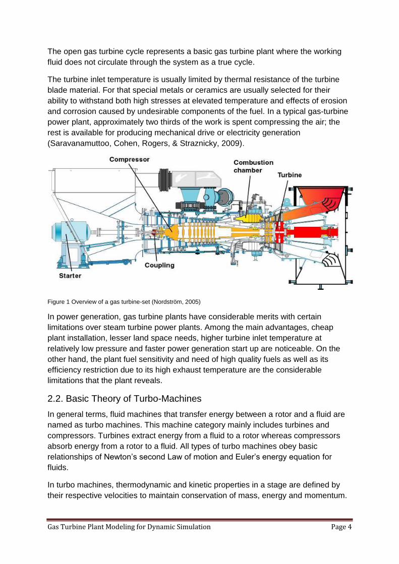
Figure 1 Overview of a gas turbine-set (Nordström, 2005)
In power generation, gas turbine plants have considerable merits with certain
limitations over steam turbine power plants. Among the main advantages, cheap
plant installation, lesser land space needs, higher turbine inlet temperature at
relatively low pressure and faster power generation start up are noticeable. On the
other hand, the plant fuel sensitivity and need of high quality fuels as well as its
efficiency restriction due to its high exhaust temperature are the considerable
limitations that the plant reveals.
2.2. Basic Theory of Turbo-Machines
In general terms, fluid machines that transfer energy between a rotor and a fluid are
named as turbo machines. This machine category mainly includes turbines and
compressors. Turbines extract energy from a fluid to a rotor whereas compressors
absorb energy from a rotor to a fluid. All types of turbo machines obey basic
relationships of Newton’s second Law of motion and Euler’s energy equation for
fluids.
In turbo machines, thermodynamic and kinetic properties in a stage are defined by
their respective velocities to maintain conservation of mass, energy and momentum.

Gas Turbine Plant Modeling for Dynamic Simulation Page 5
2.2.1. Fluid Flow Phenomena
For brief elaboration of rotor and fluid flow phenomena of a turbo machine,
compressor rotor-stator stage velocity diagram denotations and conventions are
schematized as shown in Figure 2.
A) B)
C)
Figure 2 A) Schematic presentation of compressor with inlet (1) and outlet (2); B) Compressor stage denotations illustrated by 1(rotor inlet), 2(rotor outlet) and 3(stator outlet); C) The stage velocity triangles at rotor inlet and outlet
The Figure 2C in particular, illustrates the fluid velocity distributions at stage inlet and
outlet which determine the energy transfer rate over the positions. The velocity
distributions are plotted in form of velocity triangles. These are constructed by the
tangential rotor velocity (u), the relative fluid velocity to the rotor (w) and the absolute
fluid velocity (c) to stationary frame of reference. The velocity triangles on the
compression and expansion stage lines are dependent on the aerodynamic blade
shape, configured by the blade angle, radius, length and thickness. With knowledge
of the velocity triangle, extracted or absorbed energy by a turbo machine can be
determined. This is done through determination of the total enthalpy change between
inlet and outlet of expansion or compression gas path.

Gas Turbine Plant Modeling for Dynamic Simulation Page 6
To show the inter-dependence of enthalpy and velocity triangles of a turbo machine
stage, Figure 2C can be redrawn. In Figure 3 the compressor velocity triangles at
rotor inlet and outlet from Figure 2C are redrawn as an enthalpy-entropy chart. The
overall phenomena of total and static enthalpy change together with the fluid and
rotor velocity are thus illustrated.
Figure 3: Enthalpy versus entropy air compression chart
In the chart, total and static pressures and enthalpies are plotted for conditions at
rotor inlet, rotor outlet and stator outlet. The total pressure and enthalpy at each
position is the sum of their static and kinetic values.
Where “1” determines the static rotor inlet pressure, P1 and enthalpy, h1
“01” determines the total rotor inlet pressure, P01 and enthalpy, h01
“2” determines the static rotor outlet pressure, P2 and enthalpy, h1
“02” determines the total rotor outlet pressure, P02 and enthalpy, h02
“3”determines the static stator outlet pressure, P3 and enthalpy, h3
“03” determines the total stator outlet pressure, P03 and enthalpy, h03
The absolute kinetic enthalpies are then determined from the total and static enthalpy
differences at each positions on the chart. These are represented by
,
,
at the

Gas Turbine Plant Modeling for Dynamic Simulation Page 7
respective stage positions. The relative kinetic specific enthalpies are represented
by
,
and the tangential by
,
at the rotor inlet and outlet respectively.
Based on the velocity and pressure distribution on a stage, conservation of mass,
energy and momentum are combined for determination of the energy rate absorbed
or extracted by the stage.
2.2.2. Balance Equations
Conservation of mass is maintained by taking the sum of mass flow rates over all
boundaries equal to the change in mass in the control volume
[1]
In a steady-state process, mass in the turbo machine is constant over time. Thus,
[2]
Conservation of mass over a turbo machine control volume can be written as inflow
(1) and outflow (2) in equation [3].
[3]
The first law of thermodynamics states that energy must be preserved. In equation
[4], a change in internal energy is given by the difference between the heat supplied
to the system (Q) and the work performed by the system (W).
[4]
This gives:
[5]
Where dh0 is the change in total enthalpy and the term represents the change in
specific potential energy. Except for turbo machines that drive incompressible fluids,
the latter can be neglected. Furthermore, for process simplification, turbo machine
compression and expansion processes can often be assumed as adiabatic. This
gives the conservation of energy for a steady state process as:
[6]
In turbo machines, it is worth to note that work producing machines, turbines have
> , thus resulting in positive work output >0. In contrast, work absorbing
machines, compressors have < resulting in negative work output < 0.
Gas Turbine Plant Modeling for Dynamic Simulation Page 8
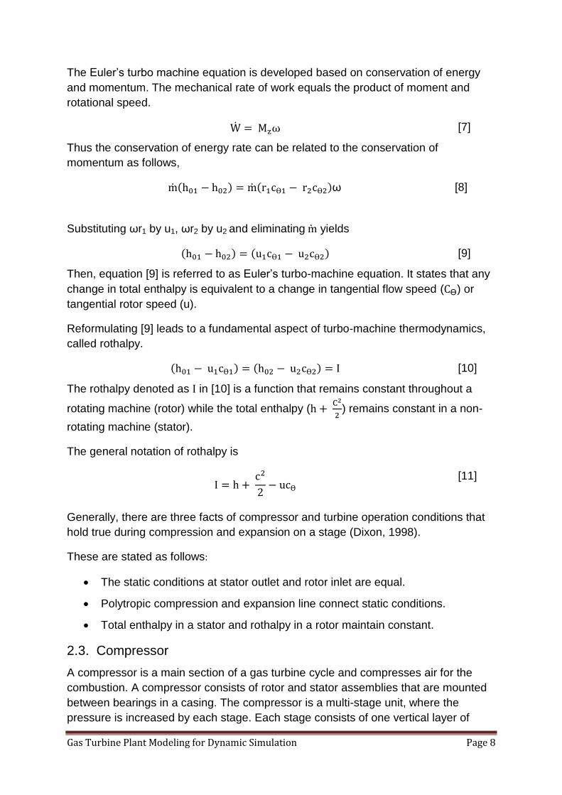
The Euler’s turbo machine equation is developed based on conservation of energy
and momentum. The mechanical rate of work equals the product of moment and
rotational speed.
[7]
Thus the conservation of energy rate can be related to the conservation of
momentum as follows,
[8]
Substituting ωr1 by u1, ωr2 by u2 and eliminating yields
[9]
Then, equation [9] is referred to as Euler’s turbo-machine equation. It states that any
change in total enthalpy is equivalent to a change in tangential flow speed ( ) or
tangential rotor speed (u).
Reformulating [9] leads to a fundamental aspect of turbo-machine thermodynamics,
called rothalpy.
[10]
The rothalpy denoted as in [10] is a function that remains constant throughout a
rotating machine (rotor) while the total enthalpy (
) remains constant in a non-
rotating machine (stator).
The general notation of rothalpy is
[11]
Generally, there are three facts of compressor and turbine operation conditions that
hold true during compression and expansion on a stage (Dixon, 1998).
These are stated as follows:
The static conditions at stator outlet and rotor inlet are equal.
Polytropic compression and expansion line connect static conditions.
Total enthalpy in a stator and rothalpy in a rotor maintain constant.
2.3. Compressor
A compressor is a main section of a gas turbine cycle and compresses air for the
combustion. A compressor consists of rotor and stator assemblies that are mounted
between bearings in a casing. The compressor is a multi-stage unit, where the
pressure is increased by each stage. Each stage consists of one vertical layer of
ω

Gas Turbine Plant Modeling for Dynamic Simulation Page 9
rotating blades, and stator vanes. The stator vanes decrease the air velocity and turn
it into static pressure. Besides, the stators lead the airflow at a correct angle to the
next stage of rotor blades. Sealing between the stages prevent the air from leaking.
Owing to the decreasing pattern of the cross section area of the airflow from inlet to
outlet, the axial velocity remains constant as the volume decreases during the
compression.
At start of the compressor operation, ambient air is taken through an inlet duct and
passes a filter before reaching the compressor. The importance of the filter is to
prevent objects from entering the compressor and minimize erosion and corrosion.
Otherwise, entry of unwanted object creates rotor blade twist that possibly turns the
compressor to break down due to minimum air flow intake. Such effects can also
occur during compressor start-up and stop operations when the volume air flow is low
at high compression pressure ratio. These phenomena are technically named as
compressor surge or stall effect that turns the compressor to oscillate.
In principle, surging is when the airflow through the whole compressor is stopped;
stall effect is when only some stages are affected by flow break up. As the result, the
oscillation due to stalling can damage the compressor since it creates stress on the
blades.
To alleviate the consequence of surging, variable guide vanes together with bleed
valves are used to optimize for full load operating mode. The variable inlet guide
vanes are airflow guiders and adjustable to the rotor inlet blade angle for flow control.
The term variable inlet guide vane (VIGV) refers specifically to the row of variable
vanes at the entry of a compressor. The function of such VIGV’s is to improve the
aerodynamic stability of the compressor when it is operating at relatively low
rotational speed or air mass flow rate at off-design (Saravanamuttoo, Cohen, Rogers,
& Straznicky, 2009).
At low speed and mass flow conditions, the variable vanes are in a near closed
position, directing and turning the airflow in the direction of rotation of the rotor blades
immediately downstream. This reduces the fluid inlet angle at the entry to the blades
and the tendency of them to stall as well. As the rotational speed and mass flow of
the compressor increases with increasing engine power, the vanes are moved
progressively and in harmony towards an optimum open position.

Gas Turbine Plant Modeling for Dynamic Simulation Page 10
Figure 4 Compressor detailed internal blade view (Rolls-Royce, 1992)
When gas turbine power plants are operating at constant rotor speed, the variable
inlet guide vanes are deviating to be positioned at optimum angle of incidence to the
rotor inlet. By this, the rotor tangential speed (u) is maintained constant and the
aerodynamic stability of the compressor at different part load operation is preserved.
The compressor flow coefficient is described as ratio of axial air flow velocity and the
tangential rotor velocity.
[12]
From the conservation of energy, an equation can be derived that describes the
specific work required to achieve a certain pressure ratio over the compressor at a
given temperature.
There are some properties of a compressor that cannot be easily calculated
analytically, e.g. the isentropic efficiency and the mass flow through the compressor.
These must instead come from measured data, given in the form of a compressor
map. In the map, the mass flow and efficiency are listed for different values of speed
and pressure ratio. In order to reduce the number of variables needed to represent
the map, the non-dimensional variables pressure ratio, corrected speed and
corrected mass flow are used. The variables are normalized with the inlet
temperature and inlet/outlet pressures during the experiments (Saravanamuttoo,
Cohen, Rogers, & Straznicky, 2009).
[13]
Gas Turbine Plant Modeling for Dynamic Simulation Page 11
[14]
[15]
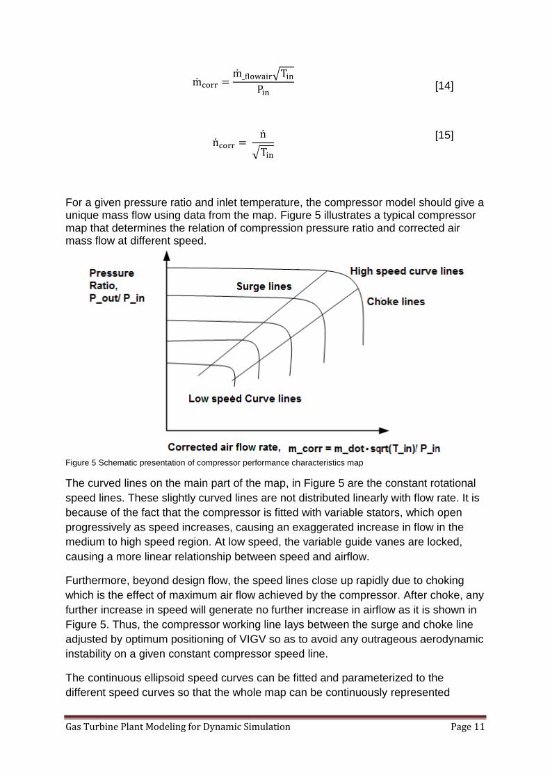
For a given pressure ratio and inlet temperature, the compressor model should give a unique mass flow using data from the map. Figure 5 illustrates a typical compressor map that determines the relation of compression pressure ratio and corrected air mass flow at different speed.
Figure 5 Schematic presentation of compressor performance characteristics map
The curved lines on the main part of the map, in Figure 5 are the constant rotational
speed lines. These slightly curved lines are not distributed linearly with flow rate. It is
because of the fact that the compressor is fitted with variable stators, which open
progressively as speed increases, causing an exaggerated increase in flow in the
medium to high speed region. At low speed, the variable guide vanes are locked,
causing a more linear relationship between speed and airflow.
Furthermore, beyond design flow, the speed lines close up rapidly due to choking
which is the effect of maximum air flow achieved by the compressor. After choke, any
further increase in speed will generate no further increase in airflow as it is shown in
Figure 5. Thus, the compressor working line lays between the surge and choke line
adjusted by optimum positioning of VIGV so as to avoid any outrageous aerodynamic
instability on a given constant compressor speed line.
The continuous ellipsoid speed curves can be fitted and parameterized to the
different speed curves so that the whole map can be continuously represented

Gas Turbine Plant Modeling for Dynamic Simulation Page 12
(Gustafsson, 1998). For each speed curve, one set of these parameters are
calculated to make the model continuous in respect to speed based on these discrete
sets of parameters. The parameters are fitted as polynomial functions of speed.
Figure 6 Ellipsoid curve for one particular speed of rotation
The curve in Figure 6 describes the curve for one speed and can be approximated as
an ellipsoid curve and represented with an ellipsoid equation which relates the mass
flow rate and pressure ratio in the constant speed line (Gustafsson, 1998). This is
simplified as [16]
[
[16]
Where = compressor machine constant which depends on the inlet geometry
and flow coefficient.
= Ambient temperature at compressor inlet
= Ambient pressure at compressor inlet
= The compression pressure ratio (
)
= the air inlet mass flow rate
For cases of isentropic compression, the compressor discharge temperature can be
calculated as follows
[17]
Gas Turbine Plant Modeling for Dynamic Simulation Page 13
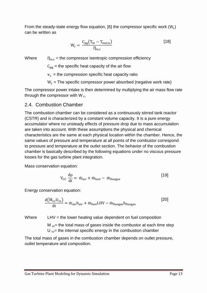
From the steady-state energy flow equation, [6] the compressor specific work ( )
can be written as
[18]
Where = the compressor isentropic compression efficiency
= the specific heat capacity of the air flow
= the compression specific heat capacity ratio
= The specific compressor power absorbed (negative work rate)
The compressor power intake is then determined by multiplying the air mass flow rate
through the compressor with W c.
2.4. Combustion Chamber
The combustion chamber can be considered as a continuously stirred tank reactor
(CSTR) and is characterized by a constant volume capacity. It is a pure energy
accumulator where no unsteady effects of pressure drop due to mass accumulation
are taken into account. With these assumptions the physical and chemical
characteristics are the same at each physical location within the chamber. Hence, the
same values of pressure and temperature at all points of the combustor correspond
to pressure and temperature at the outlet section. The behavior of the combustion
chamber is basically described by the following equations under no viscous pressure
losses for the gas turbine plant integration.
Mass conservation equation:
[19]
Energy conservation equation:
[20]
Where LHV = the lower heating value dependent on fuel composition
M cc= the total mass of gases inside the combustor at each time step
U cc= the internal specific energy in the combustion chamber
The total mass of gases in the combustion chamber depends on outlet pressure,
outlet temperature and composition.
Gas Turbine Plant Modeling for Dynamic Simulation Page 14
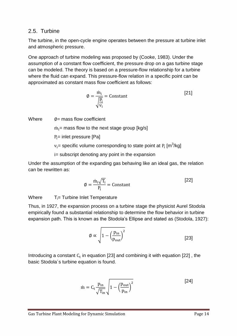
2.5. Turbine
The turbine, in the open-cycle engine operates between the pressure at turbine inlet
and atmospheric pressure.
One approach of turbine modeling was proposed by (Cooke, 1983). Under the
assumption of a constant flow coefficient, the pressure drop on a gas turbine stage
can be modeled. The theory is based on a pressure-flow relationship for a turbine
where the fluid can expand. This pressure-flow relation in a specific point can be
approximated as constant mass flow coefficient as follows:
[21]
Where = mass flow coefficient
= mass flow to the next stage group [kg/s]
= inlet pressure [Pa]
= specific volume corresponding to state point at [m3/kg]
= subscript denoting any point in the expansion
Under the assumption of the expanding gas behaving like an ideal gas, the relation
can be rewritten as:
[22]
Where Ti= Turbine Inlet Temperature
Thus, in 1927, the expansion process on a turbine stage the physicist Aurel Stodola
empirically found a substantial relationship to determine the flow behavior in turbine
expansion path. This is known as the Stodola’s Ellipse and stated as (Stodola, 1927):
[23]
Introducing a constant in equation [23] and combining it with equation [22] , the
basic Stodola´s turbine equation is found.
[24]

Gas Turbine Plant Modeling for Dynamic Simulation Page 15
Where is Stodola’s turbine constant, which is a measure of the effective flow area
through the turbine and calculated by: -
[25]
Where = flow coefficient
= turbine constriction cross-section
= number of stages
= molar gas constant
If the turbine can be considered isentropic, the discharge temperature can be written
as
[26]
From the steady-flow energy equation [6], the turbine specific work ( ) can be
written as
[27]
Where = the turbine isentropic efficiency
= the specific heat capacity of the flue gas calculated at state
condition of the expansion gas line
ɤ t = the turbine expansion specific heat ratio
= the specific turbine power extracted (positive work rate)
The turbine power output is then determined by multiplying the mass flow rate of
combustion gas flowing through the turbine with Wt.
The net power output of the gas turbine set, P net is influenced by the mass of air
processed and can be calculated as
[28]
And the thermal efficiency of the engine set will be
[29]
Where f = the fuel to air ratio
= the fuel flow rate to combustor
LHV = the lower heating value of the fuel

Gas Turbine Plant Modeling for Dynamic Simulation Page 16
= the net power output of the gas turbine set
= the total thermal of the gas turbine plant
Power turbines are often designed to have repetition stages. This means that stages
have the same geometry, a constant flow coefficient and a swirl free inflow condition.
Thus, the stage absolute inlet velocity C1 and outlet velocity C3 remain constant at
design condition. However, while at start-up and full load operation conditions, the
velocity (kinetic demolition) can create a pressure drop in the expansion path. This
creates shock on the turbine stage in form of vibration due to stage profile
(mechanical) loss.
2.6. Gas Turbine Power Loss Calculations
In complete gas turbine dimensional modeling, the stage profile loss is taken as a
sum loss on stator and rotor. The reason for doing so is to be able to relate losses to
geometrical properties such as the deviation of the flow in each blade row
(Soderberg, 1949).
The losses in the stator and the rotor respectively are expressed by the outflow
velocities such that
[30]
[31]
Where the stator profile loss factor ( ) is calculated by:
[32]
And rotor profile loss factor (ξ ) is calculated by:
[33]
The term ( ) is the stator angle deviation and ( ) is the rotor angle deviation that
are considered in the loss factor calculations in [32] and [33].
Then, the sum of the two profile loss factors gives the total mechanical loss factor
(ξ
) that determines the stage mechanical dynamics.
[34]
However, a complete gas turbine dimensional modeling needs a lot of data which
specify thermodynamic and flow quantities along the main flow direction. Thus, most
;
Gas Turbine Plant Modeling for Dynamic Simulation Page 17
gas turbine analytical models proposed in the literature are simply design models.
Some others, however, are able to predict off-design behavior by means of zero-
dimensional models.
Zero-dimensional models are defined as models that consider only thermodynamic
transformations across the component without simulating the internal flow field.
For zero dimensional turbine modeling, the lumped effect of the dynamic mechanical
losses can be calculated from total pressure drop condition. Thus, the corresponding
velocity due to the profile loss in stator and rotor can be captured in a gas plenum. In
the gas plenum, the essential aspects of stage dynamic effects are characterized by
one main equation which is composed of the physical variables. Accordingly, it has
been derived for the transient flow across the gas plenum by which pressure
variations due to mass accumulation can be calculated (Liepmann & Roshko, 1957).
[35]
[36]
And, the mechanical energy loss rate will be:
[37]
Where ΔP = the total pressure drop due to profile loss
CmL= the velocity lost in turbine shock (vibration)
=average stage profile loss factor
ρ = the medium gas density
= Turbine mass flow
= the total pressure drop rate at stage outlet
= the plenum volume
= the gas specific heat capacity ratio
=the universal gas constant
= gas plenum medium temperature
The thermal losses on a stage correspond to the temperature difference between the
turbine inter-stage and the surrounding. Besides it depends on the total heat transfer
coefficient and area of the gas turbine body. The turbine body construction is
basically made with good insulation that allows a minimum heat loss to the

Gas Turbine Plant Modeling for Dynamic Simulation Page 18
surrounding. This contributes for total cycle efficiency gain. Thus, the thermal loss is
calculated by
[38]
Where U = the overall heat transfer coefficient throughout the turbine body
A = the heat transfer surface area of the turbine body
ΔT = the internal and external temperature difference
The overall energy transfer phenomenon on a turbine control volume can be
illustrated in Figure 7.
Figure 7 Energy flow phenomena on a turbine stage
The energy flow phenomenon is thus evaluated using first law of thermodynamics for
energy conservation as in equation [39]
[39]
Where = the rate of internal energy stored in the turbine
= the rate of input energy to the turbine
= the rate of energy extracted by the turbine
= the thermal energy loss to the surrounding
= the mechanical energy loss to the surrounding
2.7. Gas Turbine Design and Off-Design Simulation
Design mode simulation refers to the plant performance at full engine design operating
mode. However, real power plants do not always operate at design capacity. Thus, off design
Gas Turbine Plant Modeling for Dynamic Simulation Page 19
simulations become important in revealing the actual engine performances. Before a new
gas turbine can be designed, many alternative thermodynamic cycles are evaluated. Then, a
cycle is selected which constitutes the cycle design point (cycle reference point) of the gas
turbine. For this design point, all the mass flows, the total pressures and total temperatures
at the inlet and outlet of all components of the engine are determined.
Off design mode simulations deal with the behavior of a plant system with given geometry.
This geometry is found by running a single cycle design point. To prepare for an off-design
simulation, the component design points must be correlated with the component maps. This
can be done automatically using standard maps of gas turbines and the standard design
point settings in these maps. The maps often need to be scaled before the off-design
calculation commences in such a way that they are consistent with the cycle design point.
In recent developments of GTP off design operations, systematic studies have been made to
correlate and get typical characteristics equations (Zhang & Cai, 2002). The equations can
be analyzed in terms of performance correction using compressor and turbine characteristic
curves. However, they cannot represent the general and typical performances of gas turbine
plants.
For pressure ratios different from nominal conditions, the isentropic efficiency falls below the
nominal isentropic efficiency η is. (Zhang & Cai, 2002).
For part load compressor operation, the equations have been given as:
[40]
[41]
Where Pi-cD = Pressure ratio from outlet to inlet at design operating mode
Pi-c = Pressure ratio from outlet to inlet at off design operating mode
= The air mass flow rate normalized by the design air flow rate
= The rotor speed normalized by the design rotor speed
= The compressor efficiency normalized by the design efficiency
The coefficients c1, c2, and c3 of the equation [40] are calculated by
[42]
[43]
[44]
–(
]

Gas Turbine Plant Modeling for Dynamic Simulation Page 20
According to (Zhang & Cai, 2002), the values of m and p should satisfy the equation,
to ensure appropriate shape and position of the compressor characteristic
curves. Thus, values of, m=1.06, p=0.36, C4 = 0.3 are also determined and
applicable for any compressor performance corrections in constant speed operation.
For turbine part load operation, the correcting equations have been given by:
[45]
[46]
Where = the power normalized by the design power output
= the efficiency normalized by the design efficiency
= the inlet mass flow rate normalized by the design flow rate
2.8. Gas Turbine Blade Cooling
Turbine blade cooling technology can be categorized in the two major groups, open
and closed loop cooling.
Closed loop cooling is a way of blade cooling by which the coolant passes through
the blade or vane to absorb heat and reject it outside of the expansion process.
Steam cooling injected from the steam cycle in a cogenerating power plant is a
typical example of closed Loop Cooling.
Open loop cooling is the most common way of blade cooling performed when the
coolant is injected into and mixed with the main flow stream. Air cooling is considered
as typical example of open loop cooling technology.
According to (Jordal, 2001), blade cooling is primarily used in large gas turbine power
plants which allow the use of higher turbine inlet temperature for better cycle
efficiency with low thermal stress compared to the un-cooled. However blade cooling
results in significant disadvantages stated as:
Turbine work output is decreased due to the compressed cooling air by
passing one or more stages.
Turbine work is lost due to the colder cooling air being mixed with hot gases
from the main stream, resulting in decreased enthalpy and total pressure.
Extraction of air from the compressor outlet has a risk of disturbing the flow
field into the combustion chamber.
There is less heat to recover in applications where the exhaust gases are used
since cooling effect makes the temperature of the gases leaving the turbine
lowered.

Gas Turbine Plant Modeling for Dynamic Simulation Page 21
The cost of producing the blades is increased.
2.9. Control Systems
Control systems are used in every process industry today. Besides, the strong
market, competition and environmental requirements have forced industries to
automate and optimize their systems using different control schemes. The need of an
automatic control system in a GTP plant is to handle fast process responses and
avoid large disruptions in the power generation
The most common regulator structure is the feedback control. A reference signal r (t)
is sent into the controller and compared to the process output signal y (t) that needs
to be controlled. Depending on the control error calculated as:
[47]
A control signal is calculated and sent to the process that needs to be controlled. For
better understanding of the control mechanism, see Figure 8 as an example of a
feedback loop structure.
In order to build a good controller, apart from knowing the process output signal and
reference value, good process knowledge is required.
Figure 8 Process control using feedback control
A common way of finding the dynamics of the process is disturbing the process with
a transient. The most common way of doing this in the process industry is by
introducing a step in the control signal and registering the behavior of the output
signal (Hägglund, 1997).
In process industries, the most common regulator used is the PID-controller. The
PID-controller is a relatively simple controller to tune. Furthermore, it is cheap to use
comparing to the more complex controllers. Owing to these factors industries usually
prefer to use a lot of PID-controllers instead of a few more advanced controllers
(Hägglund, 1997).
Among all these PID controllers, the P and I parts are most commonly used. Thus, in
the thesis project, the GTP model is controlled by a set of PI controllers for design
and off design simulation calculations. The mathematical formulation of the PI-
controller is

Gas Turbine Plant Modeling for Dynamic Simulation Page 22
[48]
2.10. Modelica and Dymola
The component models developed in the flue gas package are all based on the
programming language Modelica and are built in the modeling and simulating
environment, Dymola.
2.10.1. Modelica
Modelica is an object-oriented, equation-based programming language developed
with the main objective to model complex physical systems using small model
components in a wide range of engineering fields.
The models are mainly not built by algorithms as in traditional programming, but by
differential, algebraic equations (DAE) that describe the physical behavior of the
model. These equations are not solved in any predefined order but are solved based
on what information the solver has access to. This means that the solver can, and
often do, manipulate the equations during the simulation so that it can solve for the
desired variables. This is the main reason to why the models are reusable for new
plant system integration.
The Non-profit Modelica Association is also responsible for developing the free
Modelica Standard Library, which is a library of models, components, equations that
are used for the GTP modeling and simulation (Modelica, 2011).
2.10.2. Dymola
Dymola, Dynamic Modeling Laboratory, is a complete object-oriented tool for
modeling and simulation of integrated and complex systems for use within
automotive, aerospace, robotics, process and other applications. It is a commercial
environment for modeling and simulating with Modelica code and is developed by the
Swedish company Dassault Systèmes AB (Dymola-Modelica, 2011).
The Dymola environment is divided in two main windows; modeling and simulating.
The modeling window is in turn composed of two main areas; text windows for writing
Modelica code for models and a graphical interface for connecting models and
components by drag and drop. The simulation window is there to simulate the models
by numerically solving the differential-algebraic-equations (DAE) that are set up in the
models. There are a wide range of numerical solvers to choose from depending on
task preferences. In this master thesis the solver Dassl has been used.
In Solvina, power plant models are mostly developed in Dymola, Thus, other
programming software preferences have not been considered.

Gas Turbine Plant Modeling for Dynamic Simulation Page 23
2.10.3. Numeric
Most numerical solvers are produced to solve ordinary differential equations written in
the standard form.
[49]
However, they are not made for solving implicit systems of differential algebraic
equations (DAE) written in the form, [50] which arises in a lot of physical systems.
[50]
For solving these DAE systems, Dassl which is a numerical solver developed by
Sandia National Laboratories (Petzold, 1982) are used. It is a non fixed step solver
and uses backward differentiation formulas (BDF) to find the solution from one time
step to another. Depending on the behavior of the solution, Dassl uses up to five of
the previous solved time steps. The length of each step is also dependent on the
behavior of the solution.

Gas Turbine Plant Modeling for Dynamic Simulation Page 24
3. Modeling
The dynamic compressor and turbine modeling have been carried out in Dymola 7.3.
The plant components have been separately modeled using the differential-
algebraic-equations (DAE) that express each of the component’s characteristics. The
modeling has been developed on the bases of zero-dimensional mass and energy
conservation equations. This has been performed with the aim to simulate a GTP
model for different sets of operations. The component models have been made with
respect to dynamic properties at different load settings. Fluid-specific functions and
routines of the Modelica fluid media package have been used for all model
developments. Thus, the temperature, pressure and gas composition have been
used to calculate functions of thermo physical properties. Enthalpy, specific heat
capacity, density are the main gas line properties that have been determined for
model developments. Continuous testing and evaluation during the modeling phase
have been performed to ensure that each component reveals substantial behavior of
the GTP model.
3.1. Compressor Modeling
The dynamic compressor model has been developed based on two harmonizing
blocks. The first model block has been made for the stage compression on steady-
state basis. This has been done in such a way that steady-state pressure ratio and
efficiency are calculated from air corrected mass flow at constant rotating speed. To
account for the performance correction, curve fitting polynomial equations from
compressor map have been implemented in the steady state stage modeling.
The above considerations have been done disregarding any dynamic effects
affecting mass and energy conservation. For that a second block, a plenum has been
modeled to make up the dynamic effects of compressor stage at the compressor
discharge section. The plenum has been modeled to be integrated at the stage exit
and represent for passage where the air velocity is nearly diffused to be low enough
as to neglect momentum variations. Thus, conservation of energy, and therefore
temperature, and pressure across this component has been considered.
3.1.1. Compressor Stage Modeling for Steady State Performance
The compressor stage for steady state performance is normally considered adiabatic.
However, the heat loss cannot always be neglected. Thus, quasi-steady-state
conditions have been assumed for the adiabatic thermodynamic equation. Besides,
the compressor operative characteristics applications in order to consider correction
during part load operation have taken part. Thus, the model has been composed of
compressor characteristic equations that provide correction on pressure ratio and
mass flow rate which in turn corrects the part load efficiency.
In this model, coefficients c1, c2 and c3 of the performance correction equation [40]
have been calculated using equations [42], [43] and [44] respectively. Thus, c1 = -
55.56, c2 = 97.78 and c3 = -41.22 have been used. At the same time values of m and

Gas Turbine Plant Modeling for Dynamic Simulation Page 25
p have been given in section 2.7 to satisfy the equation,
for appropriate
shape and position of the curves; as well as c4. Thus, for the compressor modeling,
m=1.06, p=0.36, c4 = 0.3 and have been assigned to be substituted in
equations [40] and [41]. Then, the compressor pressure ratio and efficiency
correction equation have been rearranged and implemented in stage modeling as
[51]
[52]
The efficiency of the compressor has then been corrected under the quasi-steady
assumption at each spot of the compression line.
In the model, air mass flow rate has also been calculated and given by
[53]
[54]
[55]
Where flowair is the air inlet mass flow rate; φ c the compressor flow coefficient; Fm,
compressor geometry factor and assumed to be 0.03 as Stodola’s turbine machine
constant, and Pi-c is outlet-to-inlet pressure ratio. The compressor machine constant,
corresponds to turbine matching.
The power consumption of the compressor has been calculated as the product of air
mass flow and enthalpy rise between inlet and outlet sections.
Thus, the negative power output of the compressor can be written as:
[56]
Where hin and hout represent the input and output air enthalpy. Enthalpy is a function
of temperature, pressure and air composition and can be evaluated by fluid-specific
functions and routines of the Modelica fluid media package.
The outlet flow temperature was calculated assuming an adiabatic, non-isentropic
transformation
Gas Turbine Plant Modeling for Dynamic Simulation Page 26
[57]
The specific heat capacity Cp and specific heat ratio ɤ were calculated at the state
medium temperature and pressure at the inlet and outlet sections of the compressor.
The above calculations were made disregarding the effects of mass accumulation.
However, these effects must be included in a dynamic simulation and, therefore, a
plenum was modeled at the compressor discharge section to account for them.
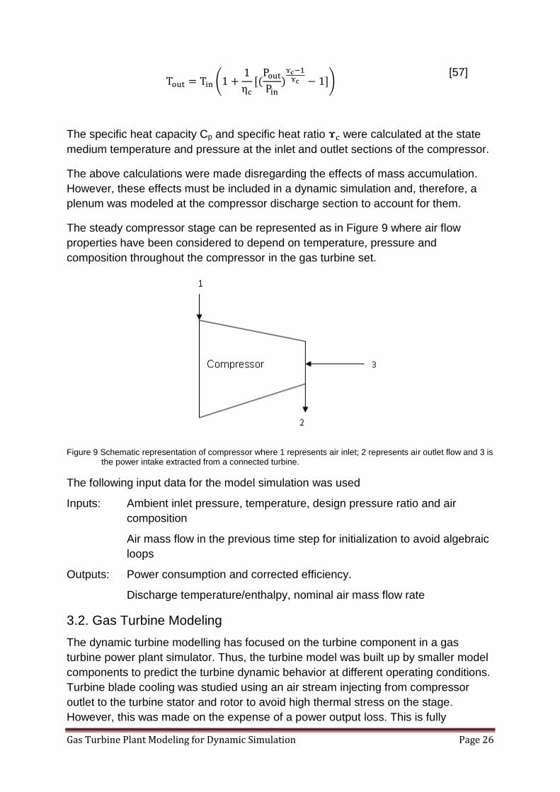
The steady compressor stage can be represented as in Figure 9 where air flow
properties have been considered to depend on temperature, pressure and
composition throughout the compressor in the gas turbine set.
Figure 9 Schematic representation of compressor where 1 represents air inlet; 2 represents air outlet flow and 3 is the power intake extracted from a connected turbine.
The following input data for the model simulation was used
Inputs: Ambient inlet pressure, temperature, design pressure ratio and air
composition
Air mass flow in the previous time step for initialization to avoid algebraic
loops
Outputs: Power consumption and corrected efficiency.
Discharge temperature/enthalpy, nominal air mass flow rate
3.2. Gas Turbine Modeling
The dynamic turbine modelling has focused on the turbine component in a gas
turbine power plant simulator. Thus, the turbine model was built up by smaller model
components to predict the turbine dynamic behavior at different operating conditions.
Turbine blade cooling was studied using an air stream injecting from compressor
outlet to the turbine stator and rotor to avoid high thermal stress on the stage.
However, this was made on the expense of a power output loss. This is fully
Gas Turbine Plant Modeling for Dynamic Simulation Page 27
consistent with the conclusions of (Jordal, 2001) that for low and medium gas turbine
power plants, blade cooling can be omitted.
3.2.1. Air-Cooling Passage Modeling
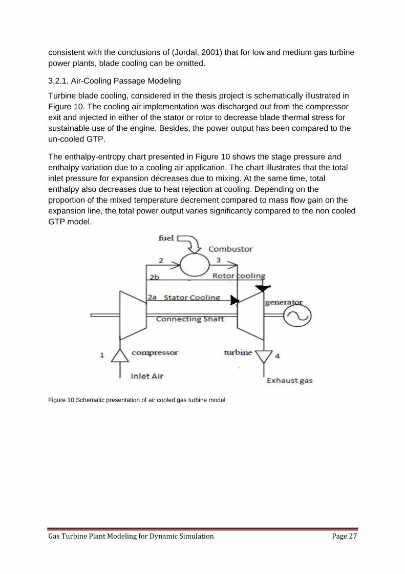
Turbine blade cooling, considered in the thesis project is schematically illustrated in
Figure 10. The cooling air implementation was discharged out from the compressor
exit and injected in either of the stator or rotor to decrease blade thermal stress for
sustainable use of the engine. Besides, the power output has been compared to the
un-cooled GTP.
The enthalpy-entropy chart presented in Figure 10 shows the stage pressure and
enthalpy variation due to a cooling air application. The chart illustrates that the total
inlet pressure for expansion decreases due to mixing. At the same time, total
enthalpy also decreases due to heat rejection at cooling. Depending on the
proportion of the mixed temperature decrement compared to mass flow gain on the
expansion line, the total power output varies significantly compared to the non cooled
GTP model.
Figure 10 Schematic presentation of air cooled gas turbine model
Gas Turbine Plant Modeling for Dynamic Simulation Page 28
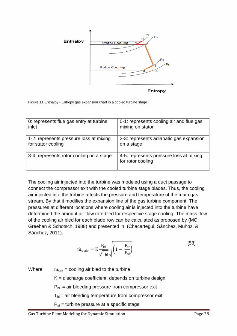
Figure 11 Enthalpy - Entropy gas expansion chart in a cooled turbine stage
0: represents flue gas entry at turbine inlet
0-1: represents cooling air and flue gas mixing on stator
1-2: represents pressure loss at mixing for stator cooling
2-3: represents adiabatic gas expansion on a stage
3-4: represents rotor cooling on a stage 4-5: represents pressure loss at mixing for rotor cooling
The cooling air injected into the turbine was modeled using a duct passage to
connect the compressor exit with the cooled turbine stage blades. Thus, the cooling
air injected into the turbine affects the pressure and temperature of the main gas
stream. By that it modifies the expansion line of the gas turbine component. The
pressures at different locations where cooling air is injected into the turbine have
determined the amount air flow rate bled for respective stage cooling. The mass flow
of the cooling air bled for each blade row can be calculated as proposed by (MC
Greehan & Schotsch, 1988) and presented in (Chacartegui, Sánchez, Muñoz, &
Sánchez, 2011).
[58]
Where cair = cooling air bled to the turbine
K = discharge coefficient, depends on turbine design
PbL = air bleeding pressure from compressor exit
Tbl = air bleeding temperature from compressor exit
Pst = turbine pressure at a specific stage

Gas Turbine Plant Modeling for Dynamic Simulation Page 29
In the air-cooling injecting duct model development, the above equation was
implemented as the main model equation. It was used for maintaining mass and
energy conservation when mixing of cooling air and the main gas stream were
considered during the dynamic gas turbine simulation.
3.2.2. Turbine Stage Modeling for Steady State Performance
From a thermodynamic point of view, cooled turbine stages cannot be considered as
an adiabatic machine. In order to determine the starting point of the expansion line,
pressure and temperature are needed at this location. Both parameters are linked to
the mass flow of combustion gases through the flow parameter, whose value is
determined at on design operating conditions (Cooke, 1983)
[59]
Where min = is the turbine inlet mass flow rate
Tin = the turbine inlet temperature
Pi-t = the turbine outlet to inlet pressure ratio
And is Stodola’s turbine constant, which is a measure of the effective flow area
through the turbine.
Starting from these initial conditions, the expansion gas line of the turbine was used
to evaluate enthalpy variations for useful work determination. It also helped in
calculating the pressures at different locations where cooling air was injected into the
turbine.
The model was developed to evaluate the quasi-steady state performance of the gas
turbine stage; with assumption of no mass accumulation on the turbine stage. The
expansion line of the turbine was constructed with a method proposed by (EL Masri,
1986).
Furthermore, the model was used for simulation of the gas turbine performance with
and without stage cooling implementation. The gas inlet temperature has an
influence on consideration of stage cooling to protect the turbine blades from thermal
stress and erosion.
During the cooled stage modeling, connection of an air nozzle component to the inlet
of the gas turbine stage was considered. By that the mixed output temperature was
taken as inlet turbine temperature for adiabatic non isentropic expansion.
Then, mass and energy conservation of stage mixing was calculated at constant
turbine stage pressure as follows.
[60]

Gas Turbine Plant Modeling for Dynamic Simulation Page 30
[61]
While mixing at the stator stage before expansion, a certain pressure loss due to
mixing was considered at constant total inlet condition. This is usually evaluated from
experimental data. Thus, an approximate value of 2% pressure loss from inlet port
pressure was taken as default parametric value to calculate the inlet expansion
pressure. The same pressure loss was implemented as well for rotor cooling. The
pressure loss percentage was also used in the gas turbine model developed by
(Chacartegui, Sánchez, Muñoz, & Sánchez, 2011).
The model also considered turbine performance correction using equations [45] and
[46] in section 2.7 that provide mass flow rate and the part load efficiency corrections.
Thus, the expansion process considered the corrected isentropic efficiency, pressure
ratio and mass flow rate as state variables. With these, it was able to determine the
thermo physical properties at the inlet and outlet of the expansion path. The adiabatic
non isentropic turbine expansion equation implemented was:
[62]
Where = the turbine inlet temperature
= the turbine outlet temperature
= the corrected isentropic stage efficiency
= the turbine outlet pressure
= the turbine inlet pressure
ɤ t = the specific heat ratio
Here, it is worth noting that the enthalpy of the cooling air is the same for all stages
that are considered to be cooled. This is due to the fact that the bleeding point at the
compressor discharge is the same for all air cooling nozzles that are connected to
cool turbine blades.
3.3. Gas Plenum Modeling
The gas plenum has been modeled to represent a passage at the compressor
discharge to combustion chamber and turbine inter-stage free space. The plenum
was modeled to capture the dynamic effect of stator-rotor mechanical and thermal
losses to the surrounding.
The main model equation is composed of variables that characterize the essential
aspects of stage dynamic effects in the plant simulation. Thus, conservation of

Gas Turbine Plant Modeling for Dynamic Simulation Page 31
energy, and therefore temperature, and pressure across this component is
maintained constant. The continuity equation for the unsteady-state flow across the
plenum has been used. This can be written as (Liepmann & Roshko, 1957)
[63]
Where = the volume of the free space (plenum) between each pair of turbine
stages
= rate of pressure variation at outlet port of the gas plenum to the
next turbine stage
= the inlet flue gas flow rate of the gas the plenum
= the outlet flue gas flow rate of the gas plenum
= the outlet flue gas temperature to the next turbine stage
= the specific heat capacity ratio
R = the universal gas constant calculated at the plenum temperature and
pressure and gas composition
Using [63], pressure variations due to mass accumulation in the compressor and
turbine passages, transition duct and combustor can be calculated. The performance
of the model was tested by connecting two steady-state gas turbine stages with the
gas plenum model. It was possible to capture the mechanical and thermal losses to
the surrounding using the heat ports. The mechanical loss corresponds to the profile
losses that create shock on the stage and result in stage vibration. The thermal loss
was evaluated considering the thermal resistance of turbine body and the
surrounding temperature.
3.4. Model Integrations for GTP Simulation
In this section, the model components of the compressor and turbine have been
separately built and simulated to test before they were brought for gas generating
unit/plant integration. Then, gas turbine unit has been integrated with the tested
compressor, existing verified combustion chamber and turbine models with all the
auxiliary component models. Air to fuel ratio calculator to consider stoichiometric
combustion and air cooling passage have been the major auxiliary models integrated
for the required operation condition. The testing has been carried out by setting inlet
and outlet boundary conditions on models. The unsteady/transient effects in the
compression and expansion paths have been captured in the plenum model
integrated with the steady stage models.
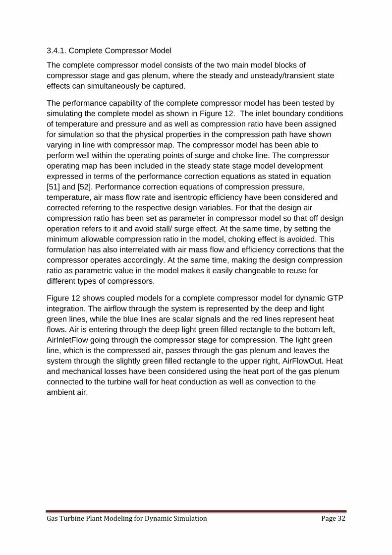
Gas Turbine Plant Modeling for Dynamic Simulation Page 32
3.4.1. Complete Compressor Model
The complete compressor model consists of the two main model blocks of
compressor stage and gas plenum, where the steady and unsteady/transient state
effects can simultaneously be captured.
The performance capability of the complete compressor model has been tested by
simulating the complete model as shown in Figure 12. The inlet boundary conditions
of temperature and pressure and as well as compression ratio have been assigned
for simulation so that the physical properties in the compression path have shown
varying in line with compressor map. The compressor model has been able to
perform well within the operating points of surge and choke line. The compressor
operating map has been included in the steady state stage model development
expressed in terms of the performance correction equations as stated in equation
[51] and [52]. Performance correction equations of compression pressure,
temperature, air mass flow rate and isentropic efficiency have been considered and
corrected referring to the respective design variables. For that the design air
compression ratio has been set as parameter in compressor model so that off design
operation refers to it and avoid stall/ surge effect. At the same time, by setting the
minimum allowable compression ratio in the model, choking effect is avoided. This
formulation has also interrelated with air mass flow and efficiency corrections that the
compressor operates accordingly. At the same time, making the design compression
ratio as parametric value in the model makes it easily changeable to reuse for
different types of compressors.
Figure 12 shows coupled models for a complete compressor model for dynamic GTP
integration. The airflow through the system is represented by the deep and light
green lines, while the blue lines are scalar signals and the red lines represent heat
flows. Air is entering through the deep light green filled rectangle to the bottom left,
AirInletFlow going through the compressor stage for compression. The light green
line, which is the compressed air, passes through the gas plenum and leaves the
system through the slightly green filled rectangle to the upper right, AirFlowOut. Heat
and mechanical losses have been considered using the heat port of the gas plenum
connected to the turbine wall for heat conduction as well as convection to the
ambient air.

Gas Turbine Plant Modeling for Dynamic Simulation Page 33
Figure 12 Complete Compressor Integrated model
3.4.2. Complete Turbine Model
The complete turbine model consists of the two main model blocks turbine stage and
gas plenum, where the steady and unsteady state effects can simultaneously be
captured.
Complete two stage turbines have been integrated for model comparion test. Exiting
static Stodola’s turbine and the newly developed dynamic turbine stages have been
simulated for performance comparison. For both simulation test cases, boundary inlet
conditions of design expansion ratio and turbine temperature have been assigned.
The simulation results have then been plotted to analyze the inter-relatedness of the
gas expansion properties with respect to mass flow, power output and efficiency
correction. Off design turbine performance has also been tested in order to analyze
result variations from the design operating mode. Change in turbine inlet pressure
has been done to examine off design operation at constant turbine inlet temperature.
In the simulation, inputs of design turbine pressure ratio and inlet temperature have
first been considered for determination of nominal turbine inlet mass flow rate using
Stodola’s relation equation [24]. Then, in the model the design inlet mass flow rate
has been used as default parameter for cases of performance correction calculations
that have gone off design operating mode.
Figure 13 shows the connected models in Dymola forming a complete dynamic
turbine model with no stage cooling. The combusted flue gas flow through the system
is represented by the double deep, medium and light red lines while the blue lines

Gas Turbine Plant Modeling for Dynamic Simulation Page 34
are scalar signals and the single red lines represent heat flows to the surrounding.
Hot flue gas of double deep red line from green filled rectangle at the upper left is
entering to another green filled rectangle of the gas plenum to pass through and
account for combustion dynamics and expand on turbine stage. The double medium
red line, come out from the first stage expansion passes through the intermediate
plenum to capture the sage dynamics ; and lead to the next turbine stage for further
work extraction; and leaving the system in light red line through the green unfilled
rectangle to the bottom right. Heat and mechanical losses have been considered by
connecting the heat ports of the gas plena to the turbine wall to the ambient air for
heat convection.
Figure 13 Complete Gas Turbine model with no stage cooling
On the other hand, Figure 14 represents the connected models in Dymola forming a
complete dynamic turbine model with stage cooling by injecting air from the compressor
exit. Air cooling passages from the compressor exit have been modeled. Unsteady-air-
Plenum which captures the stage gas dynamics has been connected to AirFlowOut at the
second upper left representing the compressor steady-state stage exit. The air
bleeding passage models have been connected to the air-plenum outlet and to the
green filled rectangle of the turbine stage inlets for cooling. The rest of the model connection
is the same as complete dynamic turbine stage with no cooling.

Gas Turbine Plant Modeling for Dynamic Simulation Page 35
It’s worth noting that air bleeding passage model calculates the amount of air flow rate used
for stage cooling depending on the respective cooling stage pressure variation as described
by the model equation [58].
Figure 14 Complete cooled gas turbine Model with air-cooling from compressor exit
3.4.3. Complete GTP Model Integration for Verification
For the newly developed gas turbine plant model verification, the boundary
conditions of ambient temperature and pressure at compressor inlet and
compression ratio have been assigned. At the turbine outlet, same ambient
pressures together with temperature for simulation initialization were assigned.
Figure 15 presents the full simulation chart of GTP involving all components
necessary for the model verification. All the flow lines have been previously illustrated
in the individual compressor and turbine model integration. However, in addition, the
GTP model has also included fuel/air calculating model so as to adjust the air flow to
compressor with the required air flow for complete combustion. For the model
verification, the model simulation chart has followed the same engineering scheme
with respect to boundary condition settings as the static GT-Unit at Solvina.
Then, simulation outputs have been plotted and analyzed to compare the power
output, flue gas mass flow rate and other main variables together with captured
dynamic effects.

Gas Turbine Plant Modeling for Dynamic Simulation Page 36
The simulation results have confirmed that it has shown persistent performance in
capturing the unsteady effects in gas generation unit in line with extracting power.
Accordingly, the simulation outputs have been plotted and analyzed in result section.
Figure 15 Complete GTP simulation-chart for Verification
3.5. GTP Model for Control System Setting
The complete gas turbine plant model is built up by the complete compressor and
turbine models, together with Solvina’s existing fixed step combustor model. PI
controllers were used in this project for control of design and off-design conditions
and load adjustments. The complete plant model is also the final test of the
compressor and turbine models.
In the thesis project, the compressor and the turbine models have been developed
based on constant rotor speed operation condition. Thus, the integrated gas turbine
model has been simulated with consideration of no aerodynamic instability. For that
optimum variable inlet guide vane (VIGV) position is tuned at the compressor inlet for
constant turbine exhaust temperature to maintain the working line unchanged for all
part load operation as in (Walsh & Fletcher, 1998). Figure 16 presents the GT-Unit
integration with no turbine blade cooling and with sets of input and output interfacing
signals. In Figure 16, the inlet and outlet signals represented in blue lines have been
extended out and seen connected with PID controllers in complete GTP simulation
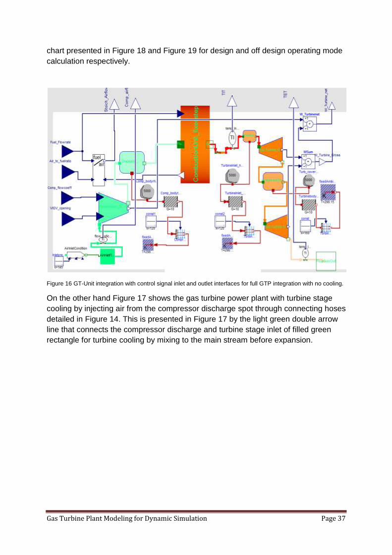
Gas Turbine Plant Modeling for Dynamic Simulation Page 37
chart presented in Figure 18 and Figure 19 for design and off design operating mode
calculation respectively.
Figure 16 GT-Unit integration with control signal inlet and outlet interfaces for full GTP integration with no cooling.
On the other hand Figure 17 shows the gas turbine power plant with turbine stage
cooling by injecting air from the compressor discharge spot through connecting hoses
detailed in Figure 14. This is presented in Figure 17 by the light green double arrow
line that connects the compressor discharge and turbine stage inlet of filled green
rectangle for turbine cooling by mixing to the main stream before expansion.

Gas Turbine Plant Modeling for Dynamic Simulation Page 38
Figure 17 GT-Unit integration with control signal inlet and outlet interfaces for full GTP integration with cooling.
3.6. GTP Model with Control System Setting
In this section, the complete gas turbine plant simulation integration is presented. The
model has been simulated both at design and off design operation modes.
3.6.1. Design Mode Simulations
In the design mode simulations, the complete gas turbine set has been simulated for
determining the design point conditions. Turbine inlet temperature, 13500c and
compression pressure ratio, 20:1 have been assigned as design point conditions of
the model. Independent variables of the gas turbine cycle are ambient conditions of
1 bar and 15oC at compressor inlet and 1 bar at turbine outlet.
The design mode simulation of the gas turbine plant has been performed using two
PI controllers. The first PI controller has been set to match the air mass flow rate
required by the combustion chamber with that of the air mass flow rate to the
compressor by tuning the design flow coefficient of the compressor. The second PI
controller has been adjusted to control the design turbine inlet temperature by
actuating the fuel consumption rate. Thereafter, simulation on the complete GTP
model has been performed in order to determine the design compressor flow
coefficient that remains constant as parameter for off design simulations. At the same
time, the power output has then been used as reference power for part load settings.
Figure 18 shows the gas turbine plant design mode simulation set up with two PID
controllers discussed above. VIGV opening to full open position, 1 and air to fuel ratio
of 1.25 have also been set in order to determine the design GTP outputs.

Gas Turbine Plant Modeling for Dynamic Simulation Page 39
Figure 18 Control System Setting for regulating design mode simulation calculation
3.6.2. Off design Mode Simulations
As all the thermodynamic design properties are known from the design simulations,
the off-design calculations can be performed so that comparable performance
deviations are observed. Various load adjustment criteria can be adopted in the plant
operation. However, in the thesis project, three simple PI controllers have been used
to analyze the GTP performance dynamics while operating in a wide range of modes.
During the tests, the plant performance dynamics has been revealed due to the inter-
dependent relations among the variables. The controllers’ set up have been
implemented in a way that the required set power is directly controlled by the fuel
mass flow rate which in turn determine the air mass flow rate for complete
combustion. Simultaneously, the air flow rate is affected by VIGV opening positions
that are tuned for constant turbine exhaust temperature, TET in constant speed part
load operations (Walsh & Fletcher, 1998). This method has been used reveal the
dynamic response of the main GTP variables being varied in power generation.
Accordingly, the part load simulations have been performed using the fuel
consumption rate to control the power output; the air flow rate to the compressor to
be controlled through the effect of fuel flow rate variation using air to fuel ratio meter
which senses the oxygen amount in the combustion chamber for complete
combustion; and the VIGV openings set to control constant TET of 6000C for all part
load simulations.
Figure 19 shows the GTP off-design simulation chart with three PID controllers set
accordingly as discussed above.

Gas Turbine Plant Modeling for Dynamic Simulation Page 40
Figure 19 Control System Setting for regulating part load operating mode
Gas Turbine Plant Modeling for Dynamic Simulation Page 41
4. Results and Discussion
4.1. Model Verification Results
In this section, simulation results of the model components developed in the thesis
project have been verified compared with that of the existing Stodola’s turbine stage
and static GT-Unit at Solvina.
4.1.1. Turbine Stage Model Verification Result
Two-turbine stages of the existing static and the newly developed dynamic models
have been simulated both at design and off design operation modes for the model
comparative verification. For the simulation start up, boundary conditions have been
set with design inlet and outlet pressure of 15 and 1 bar as well as inlet temperature
of 1400 0C. For the cooled turbine stage simulation test, cooling air bleeding from
compressor exit has also been set by boundary condition of a pressure 15.5 bar and
a temperature of 4000C. The bleeding temperature was calculated using the
adiabatic compression equation with compression pressure ratio of 15 from ambient
air condition temperature 15oc and compressor isentropic efficiency, 0.85.
Using the input values, simulations were accomplished and results have been plotted
to compare performance variable deviations at the same operation condition. Looking
into the results, the model has been put forward to be integrated in the gas turbine
plant verification for complete dynamic GTP integration. The aforementioned design
input data have been used for design mode simulation.
On the other hand, off design operating condition was performed on the existing
verified static and the newly developed complete turbine stage models through
varying the turbine inlet pressure. For that turbine inlet pressure of 10 bars has been
set on the models to examine the variation of turbine characteristic variables from the
design case operation. This has been done to reveal the steady-state properties of
the gas expansion as well as capturing the transient/dynamic effects in the
intermediate gas plenum.
With this manner, comparison of the existing static and the newly dynamic turbine
stage simulation results were plotted to compare the result variations.
Figure 20 has shown that the dynamic gas turbine stage power output has distinctive
variation over the static one. This is due to the energy and mass balance on the
expansion gas line that has been considerably done with significant amount of
pressure, stage efficiency and power correction referring to the respective design
values. Besides, the inter-stage power loss in form of mechanical and thermal has
been captured by the gas plenum. These had impact for the quasi-steady gas turbine
power output decrement compared to the static gas turbine unit at Solvina under
design and off-design operating mode.
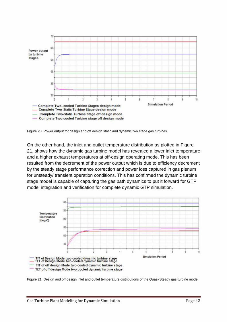
Gas Turbine Plant Modeling for Dynamic Simulation Page 42
Figure 20 Power output for design and off design static and dynamic two stage gas turbines
On the other hand, the inlet and outlet temperature distribution as plotted in Figure
21, shows how the dynamic gas turbine model has revealed a lower inlet temperature
and a higher exhaust temperatures at off-design operating mode. This has been
resulted from the decrement of the power output which is due to efficiency decrement
by the steady stage performance correction and power loss captured in gas plenum
for unsteady/ transient operation conditions. This has confirmed the dynamic turbine
stage model is capable of capturing the gas path dynamics to put it forward for GTP
model integration and verification for complete dynamic GTP simulation.
Figure 21 Design and off design inlet and outlet temperature distributions of the Quasi-Steady gas turbine model

Gas Turbine Plant Modeling for Dynamic Simulation Page 43
4.1.2. GTP Model Verification Result
For the developed gas turbine plant model verification, the same boundary conditions
have been set as the existing gas turbine unit at Solvina AB. Hence, the set up of
boundary conditions have been ambient temperature and pressure of 1 bar and 288K
at the compressor inlet and turbine outlet. Besides component parametric values
have been assigned together with initial variable values. Hence, the model
simulations have set compression ratio of 10 on the compressor model so as to
determine the power output by the gas turbine set. Then, input parameters assigned
to the total plant in the boundary and component models enable the combustion
chamber model to calculate the combustion adiabatic temperature. From the value of
the air to fuel ratio, the fuel mass flow rate and composition of the combustion
products can be evaluated by the combustion chamber model as well.
Comparable simulation result charts were plotted below so as to see the model performance with respect to the existing GT-Unit. The plots were plotted in such a way that performances of the static gas turbine unit
and the dynamic ones can easily be seen. With that the charts have shown the
power output, flue gas mass flow rate and unsteady effects of heat and mechanical
losses captured well in line with extracting power. These have been possible owing to
energy and mass balance consideration as well as efficiency corrections involved on
the air compression and the gas expansion paths of the compressor and turbine
models respectively.
Accordingly, Figure 22 presents the consistency of the model simulation result in flue
gas mass flow rate with respect to the existing GT-unit model under cooled and un-
cooled turbine stage conditions. However, Figure 23 presents the new gas turbine
stages power outputs which have explicit decrement from the existing static gas
turbine by a significant amount. This has indeed been due compression and
expansion performance correction in the by the steady stage and power loss
captured in gas plenum for unsteady/ transient operation conditions. Corresponding
differences have been resulted in stage efficiencies, temperature and pressure as
well.
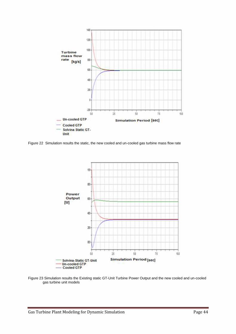
Gas Turbine Plant Modeling for Dynamic Simulation Page 44
Figure 22 Simulation results the static, the new cooled and un-cooled gas turbine mass flow rate
Figure 23 Simulation results the Existing static GT-Unit Turbine Power Output and the new cooled and un-cooled gas turbine unit models

Gas Turbine Plant Modeling for Dynamic Simulation Page 45
4.2. GTP Model Dynamic Simulation Result
Primarily, design mode simulation have been carried out in order to attain all the thermodynamic quantities calculated before performing the off-design calculations. Thus, the off-design simulation have been carried out using power output from the design mode simulation, 242MW as reference design power to adjust part load settings. In the simulation, the same independent ambient inlet and outlet conditions have been used as for the design mode simulation. Hence, simulation results have been investigated for the two part load settings at 25% and 90% of the design power output. Then,the plant output variables that determine performance characteristics have been plotted and presented below. A simulation period of 250 seconds has been set for all operation modes. A step up
in power demand of 10MW has been done after 150 seconds of simulation. This has
been done in order to observe the performance dynamics of the GTP model after
reaching steady state simulation as test to load perturbation.
Figure 24 illustrates the GTP response in power output for the required power setting
in the gas turbine control system. The corresponding fuel flow for the set power has
been tuned and plotted in Figure 25. Besides, the plots reveal the GTP model
performance dynamics regulated well after step in load perturbation on steady state
simulation at 150 sec.
Figure 24 The measured power by the GTP cycle represented by red curve line and set power for off-design simulation, shown by the blue line converge to the same value by implementing the PI controller scheme.

Gas Turbine Plant Modeling for Dynamic Simulation Page 46
Figure 25 The Power PI controller deliver a signal output of fuel flow rate to respond for the power regulation and tune the fuel flow as control variable. It further reveals the effect of the step in loading being actuated correspondingly.
At the same time, Figure 26 shows the air flow rate to the compressor leaned with the
amount of combustion air required for a given load setting. The air to fuel ratio has
been tuned by the PI controller in response to achieve the required air flow rate that
the fuel flow to the combustion chamber requires for complete combustion.
Simultaneously, constant exhaust temperature has been set for all part load
simulation controlled by the VIGV openings that in turn vary the air flow in constant
rotor speed operation.
Figure 26 The measured air flow to the compressor, red curve line and air flow rate required by the combustion chamber shown by the blue line agree and come to the same steady value by implementing the PI regulation scheme. The plot also shows the dynamic response of step in loading at 150 second in the same pattern as the main GTP model variables.
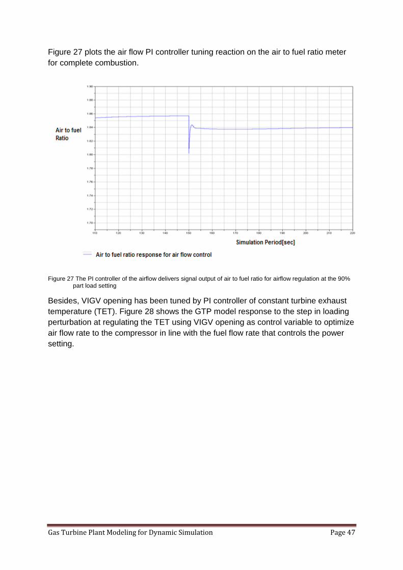
Gas Turbine Plant Modeling for Dynamic Simulation Page 47
Figure 27 plots the air flow PI controller tuning reaction on the air to fuel ratio meter
for complete combustion.
Figure 27 The PI controller of the airflow delivers signal output of air to fuel ratio for airflow regulation at the 90% part load setting
Besides, VIGV opening has been tuned by PI controller of constant turbine exhaust
temperature (TET). Figure 28 shows the GTP model response to the step in loading
perturbation at regulating the TET using VIGV opening as control variable to optimize
air flow rate to the compressor in line with the fuel flow rate that controls the power
setting.

Gas Turbine Plant Modeling for Dynamic Simulation Page 48
Figure 28 The plot illustrates the measured turbine exhaust temperature (TET), blue curve line and set TET by the red line in the off-design simulation. They converge to the same value by implementing the PI controller scheme. The TET controller has revealed the effect of the step in loading after the steady operation reached at 150 seconds.
Figure 29 The PI controller of the turbine exhaust temperature delivers signal output of VIGV opening position for the respective airflow adjustment for constant TET off design simulations. The model controller reveals the dynamic effect of step in loading after reaching steady state operation at 150seconds that confirms the GTP model robust for load perturbations.

Gas Turbine Plant Modeling for Dynamic Simulation Page 49
For further analysis and observation of the fuel flow rate variation for different load
adjustments, additional off design simulation at 25% of design power setting has
been carried out. Hence, Figure 30 presents the measured power outputs of the off
design simulations performed at 25 and 90% of the GTP design power. The
corresponding fuel flow rate at the respective loadings has been plotted in Figure 31.
Each of the simulation output variables has revealed the effect of load perturbation
after steady state operation is reached. With these, the GTP model is confirmed to be
robust for any off design simulation and can be put to replace the gas turbine process
cycle in producing electricity in GTP simulator.
Figure 30 Part load power output distribution at the respective load setting of 25% (red line) and 90% (blue line) of the design power.
Figure 31 Part load fuel consumption rate for the respective power load measured at 25%(blue line) and 90% (red line) of design power set for off-design simulations.
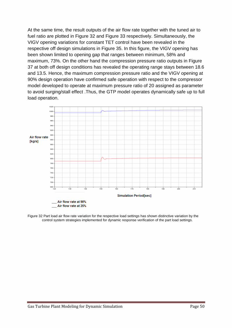
Gas Turbine Plant Modeling for Dynamic Simulation Page 50
At the same time, the result outputs of the air flow rate together with the tuned air to
fuel ratio are plotted in Figure 32 and Figure 33 respectively. Simultaneously, the
VIGV opening variations for constant TET control have been revealed in the
respective off design simulations in Figure 35. In this figure, the VIGV opening has
been shown limited to opening gap that ranges between minimum, 58% and
maximum, 73%. On the other hand the compression pressure ratio outputs in Figure
37 at both off design conditions has revealed the operating range stays between 18.6
and 13.5. Hence, the maximum compression pressure ratio and the VIGV opening at
90% design operation have confirmed safe operation with respect to the compressor
model developed to operate at maximum pressure ratio of 20 assigned as parameter
to avoid surging/stall effect .Thus, the GTP model operates dynamically safe up to full
load operation.
Figure 32 Part load air flow rate variation for the respective load settings has shown distinctive variation by the control system strategies implemented for dynamic response verification of the part load settings.
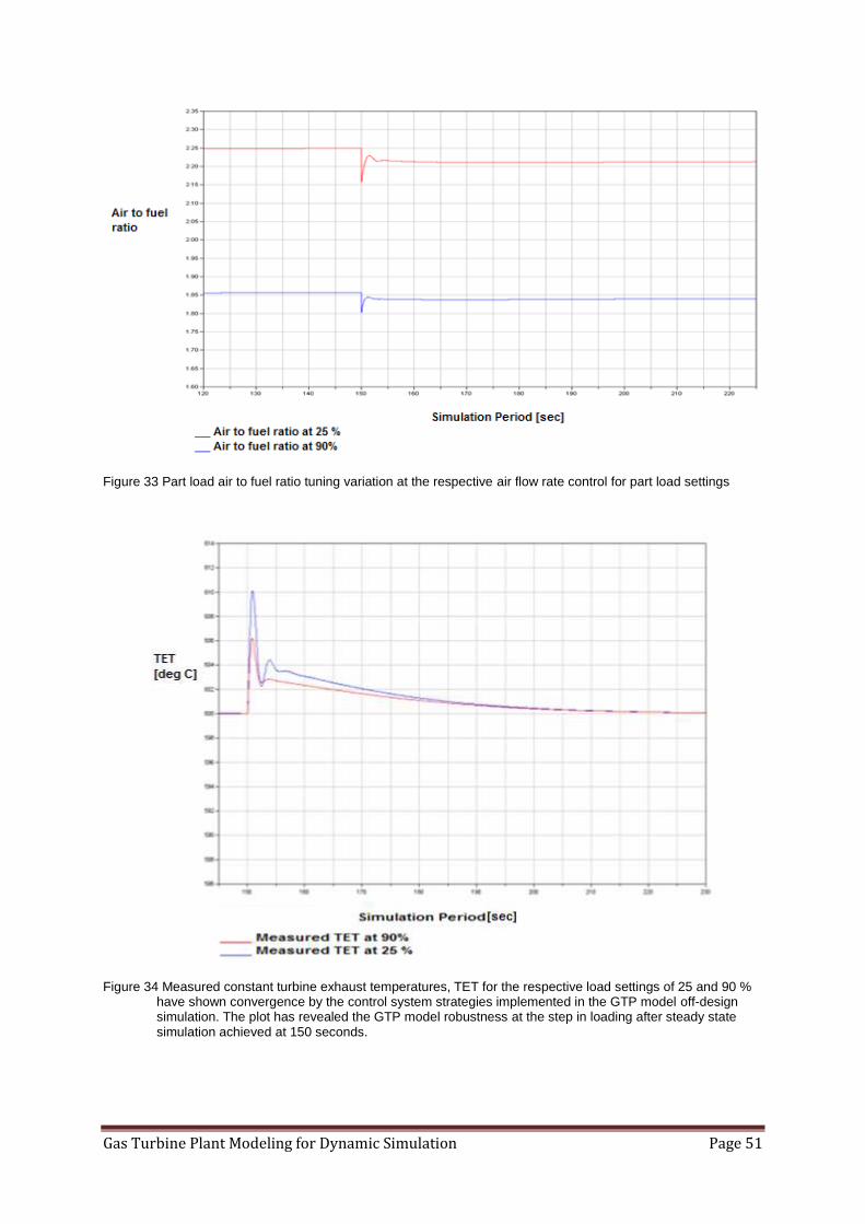
Gas Turbine Plant Modeling for Dynamic Simulation Page 51
Figure 33 Part load air to fuel ratio tuning variation at the respective air flow rate control for part load settings
Figure 34 Measured constant turbine exhaust temperatures, TET for the respective load settings of 25 and 90 % have shown convergence by the control system strategies implemented in the GTP model off-design simulation. The plot has revealed the GTP model robustness at the step in loading after steady state simulation achieved at 150 seconds.

Gas Turbine Plant Modeling for Dynamic Simulation Page 52
Figure 35 Part load VIGV tuning variation for maintaining constant TET through air flow rate variation in constant speed off-design simulation. The plot reveals its dynamic response for the the step in load perturbation implemented in the off-design simulation
In the simulation, results of the main GTP model defining variables have also been
analyzed and plotted to show their dynamic reaction over the step in loading. Thus,
turbine inlet temperature (TIT) and compression pressure ratio/combustion pressure
distribution have been plotted in Figure 36 and Figure 37 respectively during the
same test. The plots show realistic simulation results of the main GTP model
performance variables under the implementation of the control system strategy for
the off-design simulation.
Figure 36 Part load Turbine Inlet Temperature variation at the respective part load settings
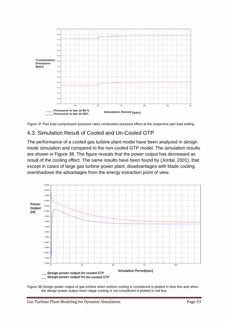
Gas Turbine Plant Modeling for Dynamic Simulation Page 53
Figure 37 Part load compression pressure ratio/ combustion pressure effect at the respective part load setting
4.3. Simulation Result of Cooled and Un-Cooled GTP
The performance of a cooled gas turbine plant model have been analyzed in design
mode simulation and compared to the non-cooled GTP model. The simulation results
are shown in Figure 38. The figure reveals that the power output has decreased as
result of the cooling effect. The same results have been found by (Jordal, 2001), that
except in cases of large gas turbine power plant, disadvantages with blade cooling
overshadows the advantages from the energy extraction point of view.
Figure 38 Design power output of gas turbine when turbine cooling is considered is plotted in blue line and when the design power output when stage cooling is not considered is plotted in red line.
Gas Turbine Plant Modeling for Dynamic Simulation Page 54
4.4. Discussion
The GTP model for dynamic GTP simulation has first been integrated and tested its performance with no control system but with boundary input values to compare with the existing static GT-Unit at Solvina. Thus, results have shown that the GTP model can play a significant role in substituting the gas generating cycle for dynamic GTP integration with control system setting. Afterwards, the GTP model simulations at design and off design mode have been performed. In the off design mode simulation, step in load perturbation have been introduced after reaching the steady-state simulation period so as to analyze and observe the model dynamic responses in its main defining variables. For that, the GTP model has been set with PI controllers that make the variables vary at different power load adjustment and show the physical dynamics correspondingly. Design mode simulation has been done with set of VIGV opening at the full position,
design compression pressure ratio and design turbine inlet temperature TIT.
The design mode simulation results have been used to set design parameters and
variables to be referred within off-design mode simulations.
Each of the off-design simulations have been done for 250 seconds. The GTP
measured values and the set values to PID controllers with PI controlling scheme
have converged to each other agreeably after dynamically responding to step in load
perturbation. The effect of the step in part load perturbation has also been revealed
in GTP variables comparatively at the same instant. These effects have been
revealed in the plots analyzed in terms of the dynamic increase in the fuel flow,
turbine inlet temperatures and compression pressure ratio.
Apparently, fuel mass flow increases uniformly by increase of the load while VIGVs is
tuned for constant TET by decreasing the air flow to the compressor in constant rotor
speed for all part load settings.
Gas turbine with blade cooling has been simulated to compare the power output. The
design mode simulation has shown that power output of the cooled turbine
decreased compared to the un-cooled GTP model. This is due to turbine work output
decrement from compressed cooling air extraction and turbine work lost due to the
main stream enthalpy and total pressure decrement at mixing. Thus, in this case,
turbine blade cooling is advised to be considered only from the material point of view.

Gas Turbine Plant Modeling for Dynamic Simulation Page 55
5. Conclusions
The GTP model has been developed thermodynamically based on zero-dimensional
conservation equations applied to each component of the engine for steady state
performance calculations and intermediate plena to account for dynamic effects.
Dymola Multi-Engineering Modeling and Simulation have been used for the model
development and simulation. Thus, high flexibility in the choice of the adjustment
criteria and model reuse is allowed by changing parameter values at the model
component according to the required operation.
Performance correction of gas turbine plant at part load operating mode has also
been considered at compressor and turbine modeling level.
Design and off-design dynamic simulations of single-shaft constant speed GTP
model have been done after the GTP model has been verified with the existing static
GT-Unit model at Solvina.
PI control systems have been used for tuning parameters in design mode and for
plant control in off-design mode.
Design point calculations on the GTP model have resulted in obtaining the gas
turbine plant general design point characteristics.
Tuning of both compressor and turbine models together in design mode simulation
has been performed so that design parameters are achieved for off design operation
reference.
GTP off-design mode simulations have been made to determine approximate plant
working line characteristics that reveal operational variations.
A gas turbine plant model has been developed and tested for its dynamic output
response at step in load perturbation after reaching steady-state simulation period.
The GTP has also found to be robust to represent the gas generating cycle to
integrate with generator as input shaft power for further inertia, mechanical and
generator efficiency consideration.
In summary, a model for dynamic simulation and analysis of gas turbine cycle is
presented in this paper. The model has proved to be good at predicting part load
analysis of the GTP. The application of the model to different power plant analyses at
different operational scenarios will lay basis for the model validation as well as
calibration for specific purpose in future works.

Gas Turbine Plant Modeling for Dynamic Simulation Page 56
6. Future Works
Implementations of simple PI controllers have been done to show the dynamic
performance variations of the gas turbine process cycle. Thus, in the future works,
The GTP model in this thesis project should be integrated with power generator
model of GTP simulator where moment of rotor inertia, mechanical and generator
efficiency are considered.
Implementation of advanced multivariable dynamic control strategies should be done
for internal and external GTP regulation. This is in order to optimize the desired
power output dependent on the main plant system variables in the gas turbine cycle,
generator and transmission grid.
Test scenarios for frequency perturbation and other abnormal effects needs to done
to validate and calibrate the plant model for specific operation

Gas Turbine Plant Modeling for Dynamic Simulation Page 57
References
Chacartegui, R., Sánchez, D., Muñoz, A., & Sánchez, T. (2011). Real time simulation
of medium size gas turbines. Energy Conversion and Management , 52 (1), 713-724.
Cooke, D. H. (1983). Modeling of off-design multistage turbine pressures by
Stodola's ellipse. Energy Incorporated, PEPSI user's group meeting. Richmond,
Virginia: Bechtel Power Corporation.
Dixon, S. L. (1998). Fluid Mechanics and Thermodynamics of Turbomachinery,
Fourth edition. Woburn, MA, USA: Butterworth-Heinemann.
Dymola-Modelica. (2011). Multi-Engineering Modeling and Simulation. Retrieved 9
2011, from Dymola-Modelica/Dynamism- Simulations-Optimization-Forecasting-
Process Control-Act-Solutions:
http://www.actsolutions.eu/Products/Dymola_Modelica_Simulation.html
EL Masri, M. (1986). On Thermodynamics of Gas Turbine Cycles: Part 2-a Model for
Expansion in Cooled Turbines. Journal of Engineering for Gas Turbines and Power ,
108 (1), 151-159.
Gustafsson, J. (1998). Static and dynamic modelling of gas turbine in advanced
cycles. Technical Report Licentiate Thesis, Lund Institute of Technology, Lund,
Sweden.
Hägglund, T. (1997). Praktisk processreglering (Second ed.). Lund, Sweden.
Jordal, K. (2001). Modeling and performance of gas turbine cycles with various
means of blade Cooling. Lund, Sweden.
Liepmann, H., & Roshko, A. (1957). Elements of gasdynamics. New York: Dover
Publications.
MC Greehan, W., & Schotsch, M. (1988). Flow characteristics of long orifices with
rotation and corner radiusing (Vol. 110). J Turbomach.
Modelica. (2011). Modelica and the Modelica Association. Retrieved 7 2011, from
https://www.modelica.org
Nordström, L. (2005). Construction of a Simulator for the Siemens Gas Turbine SGT-
600. Linköping University, Linköping.
Petzold, L. R. (1982). A Description of DASSL: A Differential/Algebraic System
Solver. Montreal, Canada: Sandia National Laboratories.
Rolls-Royce. (1992). The Jet Engine. Derby, UK: Rolls-Royce Limitted.
Saravanamuttoo, H., Cohen, H., Rogers, G., & Straznicky, P. (2009). Gas Turbine
Theory ( 6th ed.). Harlow: Pearson Education Ltd.

Gas Turbine Plant Modeling for Dynamic Simulation Page 58
Soderberg, C. (1949). Gas Turbine Laboratory. Massachusetts Institute of
Technology, Massachusetts.
Stodola, A. (1927). Steam and Gas Turbines, with a supplement on the prospects of
the thermal prime mover (Vol. 1). McGraw-Hill Book Company, Inc.
Walsh, P., & Fletcher, P. (1998). Gas Turbine Performance. Oxford, UK: Blackwell
Science Ltd.
Weston, K. C. (1992). ENERGY CONVERSION. Tusla, Oklahoma, USA.
Zhang, N., & Cai, R. (2002). Analytical solutions and typical characteristics of part-
load performances of single shaft gas turbine and its cogeneration. Energy
Conversion and Management , 43, 1323–1337.