gary l. brosch, 7-1.pdfsamuel l. zimmerman, herbert levinson.....83 our troubled planet can no...
TRANSCRIPT

Gary L. Brosch, EditorLaurel A. Land, AICP, Managing Editor
EDITORIAL BOARD
Robert B. Cervero, Ph.D. William W. MillarUniversity of California, Berkeley American Public Transportation Association
Chester E. Colby Steven E. Polzin, Ph.D., P.E.E & J Consulting University of South Florida
Gordon Fielding, Ph.D. Sandra Rosenbloom, Ph.D.University of California, Irvine University of Arizona
David J. Forkenbrock, Ph.D. Lawrence SchulmanUniversity of Iowa LS Associates
Jose A. G\mez-Ib<ñez, Ph.D. George Smerk, D.B.A.Harvard University Indiana University
Naomi W. LedJ, Ph.D.Texas Transportation Institute
The contents of this document reflect the views of the authors, who are responsible for the facts andthe accuracy of the information presented herein. This document is disseminated under thesponsorship of the U.S. Department of Transportation, University Research Institute Program, in theinterest of information exchange. The U.S. Government assumes no liability for the contents or usethereof.

SUBSCRIPTIONS
Complimentary subscriptions can be obtained by contacting:
Laurel A. Land, Managing EditorCenter for Urban Transportation Research (CUTR) • University of South Florida4202 East Fowler Avenue, CUT100 • Tampa, FL 33620-5375Phone: 813•974•1446Fax: 813•974•5168Email: [email protected]: www.nctr.usf.edu/journal.htm
SUBMISSION OF MANUSCRIPTS
The Journal of Public Transportation is a quarterly, international journal containing originalresearch and case studies associated with various forms of public transportation and relatedtransportation and policy issues. Topics are approached from a variety of academic disci-plines, including economics, engineering, planning, and others, and include policy, method-ological, technological, and financial aspects. Emphasis is placed on the identification ofinnovative solutions to transportation problems.
All articles should be approximately 4,000 words in length (18-20 double-spaced pages).Manuscripts not submitted according to the journal’s style will be returned. Submission ofthe manuscript implies commitment to publish in the journal. Papers previously publishedor under review by other journals are unacceptable. All articles are subject to peer review.Factors considered in review include validity and significance of information, substantivecontribution to the field of public transportation, and clarity and quality of presentation.Copyright is retained by the publisher, and, upon acceptance, contributions will be subjectto editorial amendment. Authors will be provided with proofs for approval prior to publi-cation.
All manuscripts must be submitted electronically, double-spaced in Word file format,containing only text and tables. If not created in Word, each table and/or chart must besubmitted separately in Excel format. All supporting illustrations and photographs must besubmitted separately in an image file format, such as TIF, JPG, AI or EPS, having a minimum300 dpi. Each chart and table must have a title and each figure must have a caption.
All manuscripts should include sections in the following order, as specified:
Cover Page - title (12 words or less) and complete contact information for all authorsFirst Page of manuscript - title and abstract (up to 150 words)Main Body - organized under section headingsReferences - Chicago Manual of Style, author-date formatBiographical Sketch - of each author
Be sure to include the author’s complete contact information, including email address,mailing address, telephone, and fax number. Submit manuscripts to the Managing Editor, asindicated above.

Volume 7, No. 1, 2004ISSN 1077-291X
The Journal of Public Transportation is published quarterly by
National Center for Transit ResearchCenter for Urban Transportation Research
University of South Florida • College of Engineering4202 East Fowler Avenue, CUT100
Tampa, Florida 33620-5375Phone: 813•974•3120
Fax: 813•974•5168Email: [email protected]
Website: www.nctr.usf.edu/journal
© 2004 Center for Urban Transportation Research
PublicTransportation
JOURNAL OF

Volume 7, No. 1, 2004ISSN 1077-291X
CONTENTS
Estimation of Bus Arrival Times Using APC DataJayakrishna Patnaik, Steven Chien, Athanassios Bladikas .................................................... 1
Determinants of Bus Dwell TimeKenneth J. Dueker, Thomas J. Kimpel, James G. Strathman, Steve Callas ................ 21
Prediction Model of Bus Arrival and Departure TimesUsing AVL and APC DataAmer Shalaby, Ali Farhan .................................................................................................................... 41
Transit Network Optimization—Minimizing Transfers and Optimizing Route DirectnessFang Zhao, Ike Ubaka ............................................................................................................................ 63
Vehicle Selection for BRT:Issues and OptionsSamuel L. Zimmerman, Herbert Levinson .................................................................................. 83
Our troubled planet can no longer afford the luxury of pursuitsconfined to an ivory tower. Scholarship has to prove its worth,
not on its own terms, but by service to the nation and the world.—Oscar Handlin
iii
Estimation of Bus Arrival Times Using APC Data
1
Estimation of Bus Arrival TimesUsing APC Data
Jayakrishna Patnaik, Steven Chien, and Athanassios BladikasNew Jersey Institute of Technology
AbstractAbstractAbstractAbstractAbstract
Bus transit operations are influenced by stochastic variations in a number of factors(e.g., traffic congestion, ridership, intersection delays, and weather conditions) thatcan force buses to deviate from their predetermined schedule and headway, resultingin deterioration of service and the lengthening of passenger waiting times for buses.Providing passengers with accurate bus arrival information through Advanced Trav-eler Information Systems can assist passengers’ decision-making (e.g., postpone de-parture time from home) and reduce average waiting time. This article develops aset of regression models that estimate arrival times for buses traveling between twopoints along a route. The data applied for developing the proposed model werecollected by Automatic Passenger Counters installed on buses operated by a transitagency in the northeast region of the United States. The results obtained are promis-ing, and indicate that the developed models could be used to estimate bus arrivaltimes under various conditions.
IntroductionPublic transportation planners and operators face increasing pressures to stimu-late patronage by providing efficient and user-friendly service. Within the contextof Intelligent Transportation Systems (ITS), Advanced Public Transportation Sys-tems (APTS) and Advanced Traveler Information Systems (ATIS) are designed tocollect, process, and disseminate real-time information to transit users via emerg-

Journal of Public Transportation, Vol. 7, No. 1, 2004
2
ing navigation and communication technologies (Federal Transit Administration1998). One of the key elements and requirements of APTS/ATIS is the ability toestimate transit vehicle arrival and/or departure times. With quickly expandingAPTS-related technologies (e.g., Global Position Systems [GPS], Automatic Ve-hicle Location Systems [AVLS] and Automatic Passenger Counting [APC] sys-tems), ATIS could provide timely vehicle arrival and/or departure information toen-route, wayside, and pretrip passengers for managing their journeys (Kalaputapuand Demetsky 1995; Abdelfattah and Khan 1998; Chien and Ding 1999; Dailey,Maclean, Cathey, and Wall 2001; Lin and Padmanabhan 2002).
To estimate vehicle arrival times, dynamic models may be developed using accu-rate data collected by new technologies (e.g., AVLS and APC). Since bus traveltimes between stops depend on a number of factors (e.g., geometric conditions,route length, number of intermediate stops and intersections, turning move-ments, incidents, etc.), stochastic traffic conditions along the route and ridershipvariation at stops further increase uncertainties. Thus, the goal of this study is theapplication of quantitative and qualitative data to develop creditable models forestimating reliable bus arrival times.
In this study, bus arrival time estimation models are developed on the basis of datacollected by APC units installed in buses. One should be surprised if a new tech-nology works exactly as intended and generates accurate data immediately after itsdeployment. APC systems should be no exception. Therefore, the purpose of thisarticle is not only to develop models for estimating bus arrival times, but also toexplore problems that could be encountered while processing data collected bythe APC units.
Literature ReviewBus arrivals at stops in urban networks are difficult to estimate because traveltimes on links, dwell times at stops, and delays at intersections fluctuate spatiallyand temporally. The joint impact of these fluctuations may cause schedule andheadway deviations as a bus moves farther from the starting terminal, therebylengthening the average waiting time for transit users and consequently degrad-ing the quality of service. A sound model, which could accurately estimate vehiclearrival times, would be capable of mitigating such impact to a large extent. How-ever, developing such a model while considering the effects of time and space,varying traffic, ridership, and weather conditions is a challenging task.
Estimation of Bus Arrival Times Using APC Data
3
AVLS, smart pager, and ATIS devices used by transit operators can provide usefulinformation. However, these devices fall short when it comes to estimating thetravel times between any two downstream stops and the arrival times at eachdownstream stop from the point of real-time observation. An arrival time estima-tion model at every downstream stop can be developed by establishing stop-to-stop travel times as a function of several significant variables (e.g., distance, num-ber of intermediate stops, total intermediate bus halting time, and time of day) tosupplement the services offered by ATIS devices (Abdelfattah and Khan 1998).
A variety of prediction models developed in previous studies were reviewed andthey can be classified into univariate and multivariate forecasting models (Chien,Ding, and Wei 2002). Univariate forecasting models are designed to predict adependent variable by describing the intrinsic relationship with its historical datamathematically. The commonly used univariate forecasting models include proba-bilistic estimation and time series models (Okutani and Stephanedes 1984;Stephanedes, Kwon, and Michalopoulos 1990; Delurgio 1998).
These methods usually have a short time lag while predicting in real-time. Theaccuracy of time series models highly relies on the similarity between real-time andhistorical traffic patterns. Variation of the historical average could cause significantinaccuracy in prediction results (Smith and Demesky 1995). Unlike univariatemodels, multivariate models can predict and explain a dependent variable on thebasis of a mathematical function of a number of independent variables. The com-monly-used multivariate models are regression models and state-space Kalmanfiltering models (Okutani and Stephanedes 1984).
Historically, regression models (both linear and nonlinear) have been popularbecause they are relatively easy to use, well established, comparable with otheravailable procedures, and well suited for parameter estimation problems.Abdelfattah and Khan (1998) developed linear and nonlinear regression modelswith simulation data to predict bus delays and the simultaneous influence ofvarious factors affecting delay. They obtained relatively promising results by usinga microsimulation approach.
In this study, regression models were developed using data collected by APC unitsinstalled in buses to estimate vehicle arrival times at all downstream stops. Thesemodels are developed using path-based data (e.g., travel time between two stopsalong the route), and the travel times are defined as a function of ridership andother external independent factors. Nonetheless, regression is not the only pos-

Journal of Public Transportation, Vol. 7, No. 1, 2004
4
sible estimation approach and other methods, such as artificial neural networks,have been explored (Chien, Ding, and Wei 2002).
Objective and ScopeThe primary objective of this study is to develop multivariate linear regressionmodels for estimating bus arrival times at major stops of a route in an urbannetwork. The study examines the methodology for developing bus arrival timeestimating models; the processing, analyzing, and refining of collected data; andthe behavior and impact of the independent variables. The scope of this studyencompasses model development and validation; analysis of variance and covari-ance and colinearity matrices of dependent and independent variables; and sug-gestions for future research on APC implementation that can benefit users andoperators.
Data CollectionPrevious studies (Abdelfattah and Khan 1998; Chien, Ding, and Wei 2002) indi-cated that bus travel times might be affected by a number of factors such as routelength, ridership (which, in turn, depends on population density and major tripgenerators), the number of stops and intersections, and the geometry of theroute. To develop a meaningful model, data collected from the study route shouldhave substantial variability in the aforementioned factors.
In this study, data was collected from APC units installed on buses operated on a30-mile (48 km) urban bus route by a transit agency in the northeast UnitedStates. Various data relating to trip information can be captured and recorded asthe bus heads out for a trip until it reaches the final destination. After the busreaches the garage/terminal, a centralized computer is engaged to transfer the tripdata recorded by the APC to the transit agency’s data center. Service along thestudied route is provided by five different patterns per each direction (e.g., in-bound and outbound) over different time periods. Patterns differ in terms ofwhere the route originates/terminates, whether or not the bus visits specific loca-tions, and the time the bus commences the trip at the origin. Because of dataavailability and sufficiency, only data collected from service patterns A and B wereused for developing bus travel time estimation models. There are 105 intendedstops in the outbound direction for each pattern. Pattern A crosses 134 intersec-tions (89 of which are signalized) and has 24 right and 23 left turns. Twelve impor-tant stops (known as time points) have been chosen for the analysis. These time

Estimation of Bus Arrival Times Using APC Data
5
points serve significant trip generators and are listed on the timetables distributedby the transit agency.
The study route operates 24 hours a day. Buses operating on different patternsmay travel different portions of the route. The 12 time points are at identicalphysical locations. The scheduled run time for the route ranges from 92 to 119minutes for the outbound trips and 78 to 113 minutes for the inbound trips. Thisstudy was based on data recorded from January through June 2002. The datacontained a total of 311 trips (including 162 outbound and 149 inbound trips)and most of the data were collected during weekday operations (including 108outbound and 96 inbound trips). In general, each trip serves more than 60 in-tended stops and 100 to 300 passengers. Data collected from outbound weekdaytrips were used to develop the proposed models for estimating bus arrival times.Table 1 illustrates the type of data collected from the APC system.
Table 1. Variables Description of APC Data

Journal of Public Transportation, Vol. 7, No. 1, 2004
6
Data Preparation for Model DevelopmentAs mentioned previously, arrival times may be influenced by traffic conditions,ridership, number of intermediate stops, and weather condition, which, in turn,may be different depending on time of day, day of the week, and pattern ID. If oneis to estimate travel times with regression models, sufficient observations (samples)should be available for developing creditable models to produce meaningful re-sults. For example, if the 108 outbound trips were grouped by different days, timeperiods, and pattern IDs, the sample size in each group would not be sufficient.Furthermore, although the actual arrival time of a bus at each time point is needed,a bus may skip a stop due to the lack of demand in some time periods. Thus, thesize of data in each group is further limited.
An attempt was made to include as many data as possible in the analysis, as will bedescribed subsequently. If a door open time was available at a time point, this wasthe arrival time used in the analysis for that time point. The distance between eachtime point and the origin is assumed as fixed with respect to each pattern ID. Thisdata was provided by the transit agency separately. The original data were furtherrefined by generating interstop travel times, actual number of stops a bus madeand the total dwell time, and number of alighting and boarding passengers be-tween two consecutive time points where the bus actually halted during everysingle trip. Based on the departure time at the first time point, trips can be groupedby time period based on their dispatching time, as indicated in Table 2, where theclassification and definition of the time periods and their break points were pro-vided by the transit agency.
Table 2. Time Periods Defined by APC Data Provider

Estimation of Bus Arrival Times Using APC Data
7
Buses departing from the first time point during different time periods may expe-rience varying traffic congestion and ridership along the route and therefore devi-ate from their schedule. For example, during the midday, people are likely to usebuses to do shopping or errands; thus, the buses may serve more stops. Also,most schools dismiss in the early afternoon, generating student ridership andschool bus traffic, causing traffic congestion. On the other hand, early morningand late night trips are likely to experience the least traffic congestion. These factssignify that time period is a significant factor associated with the estimation of bustravel times.
Whenever one uses a large database, it is desirable to screen the data carefully forerroneous entries and inconsistencies, which can be generated by equipmentmalfunction, human errors, software bugs, and other causes. Corrections andadjustments were made to the problematic data. When a correction was impos-sible, erroneous records were excluded from the analysis. Data had to be cor-rected/eliminated primarily because of the following reasons:
1. The Leg Time was reported as zero. In cases where both the door opentime at a subsequent stop and close time at the previous stop were avail-able, the difference of those times was used to compute the leg time.
2. The Stop Distance was reported as zero. Since distance is fixed betweeneach time point and the origin, such data were replaced by actual timepoint to time point distance.
3. The Open Time was blank. To get this time, the Leg Time was added to theClose Time of the immediately preceding stop.
4. The Close Time was blank. To get this time, the Dwell Time was added tothe Open Time for that stop.
5. The Stop Sequence was reported as zero. To identify the Stop Sequence (andhence the time point), the cumulative distance traveled up to that stopwas computed and compared with the known distance to the time points.If a time point could be identified, the record was kept; otherwise, it wasdropped.
6. The Open Time at a subsequent stop was earlier than the Close Time at aprevious stop. These records were dropped.
7. The Cumulative Distance from the origin to a particular stop was unusuallylonger than the average. These records were dropped.

Journal of Public Transportation, Vol. 7, No. 1, 2004
8
8. Occasionally, the Stop Distance would be unusually high. These recordswere dropped.
9. Occasionally, the bus stops (there is Dwell Time), but there are no on or offpassengers. These records were retained (particularly since Dwell Time isone of the independent variables used).
10.Occasionally, there is no Dwell Time, but there are boarding and alightingpassengers. The Dwell Time was calculated by taking the difference be-tween the Door Open Time and Door Close Time at that particular stop. Ifdoor time data were not available, the record was dropped.
11.Trip-Status (START and END) tags would show up somewhere in the middleof the trip. The tags were moved to their appropriate places.
The data were then augmented with weather information (precipitation, visibility,and wind speed) obtained from another source.
Selection of Independent VariablesThe independent variables selected to develop path-based travel time estimationmodels were distance, number of stops, dwell times, boarding and alighting pas-sengers, and weather descriptors. Furthermore, there was the option of generat-ing classes of separate models for each factor (i.e., time of day, day of week, patternID) that can affect travel time or include that factor as an independent variable inan overall regression.
The SAS (Version 8.02) package was used to develop a set of regression models.The decision on whether a model was reasonable was based on the signs of thecoefficients, values of the R-squares, t-values of the coefficients, correlation factorsamong the variables, and analysis of the residuals to indicate that the developedlinear models would be appropriate.
The analysis of the regression results indicated that weather variables were notamong the significant factors for estimating arrival times. This can be attributed tothe fact that the weather data were not sufficiently detailed or that during thestudy period the weather variations were not significant enough to have an im-pact on arrival times. A general linear model was developed for the difference ofactual and scheduled journey time with independent variables (e.g., week day,time period, weather) that were categorically chosen as class factors. To identifythe statistical insignificance of these variables, Tukey’s test (Montgomery 2001)was conducted. The p-value generated for day of the week was 0.4712, suggesting

Estimation of Bus Arrival Times Using APC Data
9
that trips taking place on different days of the week do not contribute any mea-surable difference to the travel time. These results also suggest that day of the weekis not significant as an independent variable. In addition, regression models gener-ated separately for each day of the week did not exhibit differences that could beattributed to the day. On the contrary, time of day appeared to affect travel timesignificantly, having very small p-values (< 0.0001).
Demand-related variables (number of stops, dwell times, boarding and alightingpassengers between time points) should definitely have an impact on bus traveltimes. However, it is obvious that they might be highly correlated to each other.For example, regressions were tested with different combinations of data, such as(1) stops, dwell time, boarding passengers, and alighting passengers; (2) stops,dwell times, and the sum of boarding and alighting passengers (i.e. number ofpassengers served); and (3) stops and boarding passengers. The correlation factorbetween number of passengers served and total dwell time within any pair of timepoints was as high as 0.93. Therefore, only one of these two variables was selected.Bus dwell time was chosen, as opposed to the total number of passengers served,because the count of total passengers served could be deceptive in the sense thattwo distinct activities (i.e., passengers boarding and alighting the bus) could betaking place simultaneously. Even so, dwell times at previous stops directly impactvehicle arrival times in further downstream stops. The regression that included allvariables produced R-square values that are smaller than the ones of the modelpresented here. Besides distance and time period, number of stops and durationof dwell times were the most appropriate and significant independent variableswith p-values of 0.15 or less. The proposed model has some independent variablesthat are highly correlated (e.g., dwell time and number of stops, distance andstops) and some of their coefficients do not have a very high statistical significance.
After reviewing the data, it was found that bus travel times exceed scheduled timesduring certain periods. The difference is greater if a bus was dispatched during thetime periods of late morning, mid-day and early afternoon than during morningpeak and afternoon peak. This may be due to the prohibition of street parking inthe peak hours and the presence of construction activities during nonpeak peri-ods. Due to these differences, variables associated with the time of day the triptook place (as described in Table 2), are treated as independent variables. Addi-tionally, the pattern IDs show a unique subset of stops along the route. An analysisof numerous regression results indicated that it was best to develop separatemodels for each pattern.

Journal of Public Transportation, Vol. 7, No. 1, 2004
1 0
Given the above, the general model used to estimate bus travel (and thereforearrival) time for pattern “p” from time point “i” to all downstream time points “j”is formulated as
Τi,p=b0+b1di,j+b2ti,j+b3si,j+b4Em+b5Mp+b6Lm+b7Md+b8Ea+b9Ap+b10Ev+b11Lnfor i and i + 1 ≤ j ≤ 12
where:
Ti,p is the estimated travel time from time point “i” to all downstream timepoints for bus pattern “p” (e.g., A, or B) (minutes)
di,j is the distance between TPi and TPj (miles)
ti,j
is the average of cumulative dwell time between TPi and TP
j (minutes)
si,j is the average of cumulative number of stops between TPi and TPj
Em is a binary variable that indicates Early Morning
Mp
is a binary variable that indicates Morning Peak
Lm is a binary variable that indicates Late Morning
Md
is a binary variable that indicates Mid-Day
Ea is a binary variable that indicates Early Afternoon
Ap
is a binary variable that indicates Afternoon Peak
Ev is a binary variable that indicates Evening
Ln is a binary variable that indicates Late Night
b0
is the intercept of the travel time estimation model
bk are the parameters for variables di,j, ti,j, si,j, Em, Mp, Lm, Md, Ea, Ap, Ev and Ln,respectively, where k varies from 1 to 11
i is the index of origin time points
j is the index of destination time points
Given a pattern ID, origin time point, and time period, the proposed model canestimate the required time to travel the path to every downstream time point andthereby the vehicle arrival time at that time point. All time periods are assigned a

Estimation of Bus Arrival Times Using APC Data
1 1
value of 1 if present (if the trip started in that time period), and 0 otherwise.Regressions were run both with and without intercepts. All variable notations andtheir associated coefficients are the same for both types of regression models. Theonly difference is that models having no intercepts would have their b0 valuesequal to zero.
Analysis of ResultsFor each of the two patterns used here, it is possible to develop one path-basedmodel to estimate bus travel time for all downstream time points from a givenstarting time point. It is not possible to present the results of all models in thisarticle. A sample of path-based models with intercepts for all possible origins ofPattern A is shown in Table 3. Conversely, Table 4 presents all path-based modelsof Table 3 but with no intercepts. Using the same methodology, all potentialmodels for Pattern B were also developed but are not shown here.
The models were developed using the stepwise regression method. Variables hav-ing significance level values more than 0.15 were considered to be insignificantand, hence, were not included in the model. As shown in Tables 3 and 4, the R-square values obtained ranged from 0.96 to 0.99 for all models that have inter-cepts and 0.99 for those that do not have any intercepts. The estimation of arrivaltimes is largely dependent upon the travel distance between a pair of time points.This distance was provided by the transit agency and is constant for all trips.Consequently, this results in high R-square values for all models developed. Theoverall p-values obtained for all models of both Patterns A and B is <0.0001. Theparameter estimates of morning peak, evening, and late nighttime periods arezero. This suggests that M
p, E
v, and L
n do not enter in any of the models.
Since the methodologies used to develop all models are the same, their final resultsare similar. Therefore, it is redundant to discuss each one of them individually andin detail. The plot of actual versus estimated bus travel time to all downstreamstops for Model I from Table 4 is presented in Figure 1 and the scatterplot of theresiduals in Figure 2. Both figures substantiate visually the linear relationship of thedependent variable with all independent variables that are used in the models. Inaddition, normal probability plots of the residuals (not shown here) indicate thatthe normality assumption for the distribution of residuals is not violated.
The overall model statistics for the same model (I from Table 4) are shown in thetable. The stepwise selection of variables for this model was in the order of di,j, si,j,E
a, A
p, E
m, and t
i,j. Each of these independent variables as they entered into the

Journal of Public Transportation, Vol. 7, No. 1, 2004
1 2
Figure 1. Estimated Versus Actual Travel Time (minutes)
Figure 2. Residual Plot of Estimated Travel Time (minutes)

Estimation of Bus Arrival Times Using APC Data
1 3
model retained their final p-values of <0.0001, 0.0914, <0.0001, 0.0084, 0.0002,and <0.0001, respectively. The summary statistics for each model are presented inTables 3 and 4.
Table 3. Statistics of Bus Travel Time Estimation ModelsWith Intercepts
Table 4. Statistics of Bus Travel Time Estimation ModelsWithout Intercepts

Journal of Public Transportation, Vol. 7, No. 1, 2004
1 4
As shown in Table 3, the travel time estimation model IX has a negative intercept of-2.86. However, this does not mean that the model will generate negative traveltimes. The models have positive values for the parameter estimates of variablesthat are reasonably significant contributors of the travel time estimation (e.g., di,j,ti,j, and si,j), and these variables are always positive. This suggests that the estimatednegative value of an intercept tends to act as an adjustor to the accuracy of a traveltime estimate. Therefore, under no circumstance will a travel time estimationmodel generate negative travel times. Negative signs of parameter estimates fortheir associated indicator variables representing a specific time period can be ex-plained similarly.
All models have a negative sign for some parameter estimate (e.g., b4 value forvariable E
m). This makes sense, because during early morning time periods, out-
bound buses are likely to experience less traffic congestion and, hence, shortertravel times. On the other hand, all models contained in both Tables 3 and 4always have positive signs for parameter estimates (e.g., b
8 and b
9 for variables E
a
and Ap). These results may be due to the fact that buses operating during the timeperiods of early afternoon and afternoon peak are expected to experience moretraffic congestion and are more likely to be stopped at the signalized intersections,causing longer travel times. However, another interesting observation that can bemade from these models is that some parameter estimates (e.g., b
5 for variable M
p)
have either zero or negative values. This suggests that the morning peak timeperiod either has a small or no contribution to the travel time estimation. Thismay be due to the fact that routes of Patterns A and B possibly experience lesstraffic congestion during the morning peak time period. This may be becausebuses are facing favorable signal timings and prohibition of street parking alongthe route during this time period.
A comparison of F-values of both sets of models shows that the ones that haveintercepts generate smaller values than the ones that do not have any intercepts.This is consistent with the corresponding R-square values, which are a little smallerfor models that have intercepts.
Data splitting or a cross validation approach (Snee 1977) is chosen for developingand then validating the models of Patterns A and B. These travel time estimationmodels were developed with 80 percent of the total available data for a sample size(N). The remaining 20 percent of the data were used to validate the model. Obser-vations are chosen randomly for developing and validating the models.

Estimation of Bus Arrival Times Using APC Data
1 5
Figure 3 presents statistical descriptions of the model developed using the ran-domly-selected 80 percent of the total sample data available. On the other hand,Figure 4 illustrates how the 20 percent data best fits and validates the modeldeveloped by using the other 80 percent of data. The presented statistics are forthe previously discussed Model I of Table 4. Means of actual versus estimatedtravel times for each OD pair were plotted to determine if there are any significantdifferences. Both Figures 3 and 4 point out that actual and estimated travel timesare reasonably close to each other since the observations for model development(sample size N is equal to 313) and for model validation (sample size of 76) wererandomly picked.
Figure 3. Model Development Statistics (80% of data)
As shown in Figure 4, for the OD pair TP1-TP
6, the actual standard deviation is the
highest, having a value of 12.88 minutes, while the corresponding mean actualtravel time is 51.48 minutes. This may be attributed to the fact that the availablesample size that was randomly chosen for this OD pair is very small and equal to 4.This explains why the root mean squared error for this OD pair is the highest(9.10) in spite of the fact that its estimated mean travel time is very close to the

Journal of Public Transportation, Vol. 7, No. 1, 2004
1 6
actual mean travel time. The estimated standard deviation for this OD pair is 2.45minutes.
The OD pair TP1-TP10 has the minimum sample size of 4, as did TP1-TP6. But, itsactual standard deviation is 11.53 minutes while its actual mean travel time is91.49. Proportionally (as a percent of mean) this standard deviation is approxi-mately half that of OD pair TP1-TP6. This can explain the smaller mean squarederror value for TP
1-TP
10 OD pair in comparison with the TP
1-TP
6 OD pair.
The OD pair TP1-TP12 RMSE is 8.24 (the third highest in the sequence), in spite ofits highest sample size of 13, and can be attributed to the fact that the estimatedmean travel time is essentially about 5.36 minutes higher than the actual meantravel time. The estimated standard deviations of all OD pairs vary from 1.73 to5.93 minutes, depending upon how close the downstream stops are and alsowhat their overall sample size is. Sample size varies from 4 through 13 for all ODpairs as described.
Having mentioned all these facts, it can be concluded that the results of modelvalidation using the 20 percent data are quite promising, suggesting that themodel can be appropriately used to estimate travel times with a new set of datalater. As indicated in the table and figures, the results generated by the models are
Figure 4. Model Validation Statistics (20% of data)
Estimation of Bus Arrival Times Using APC Data
1 7
very reasonable. The plots of the estimated versus actual values indicate linearrelationships. The coefficients have the anticipated signs and the adjusted R-squaresare almost 0.99 for both Patterns A and B. Some models are better than others interms of their R-squares and the statistical significance of their co-coefficients. Inall cases, the mean travel time increases as we estimate travel times to farther down-stream stops and so are their standard deviations. This makes sense, due to thefact that a bus is likely to encounter more and more stochastic traffic situations,causing delays as it moves farther away from the originating terminal.
On the basis of all developed models, a database can be generated that wouldcontain parameter estimates and values of the dependent variables for the pur-pose of estimating the travel time at downstream stops. The transit operatorwould be required to input pattern ID, stop ID, and time period. Based on theseinputs, the travel time estimation engine will select the appropriate model fromthe list of models developed to estimate the arrival times at each downstreamstop. This portion of the research will commence after all models are finalized.
Conclusions and Future ResearchOne of the major stochastic characteristics in transit operations is that vehiclearrivals tend to deviate from the posted schedule. Poor schedule or headwayadherence is undesirable for both users and operators, since it increases passengerwait/transfer times, discourages passengers from using the transit system, anddegrades operating efficiency and productivity. This study developed regressionmodels to predict bus arrival information on the basis of distance traveled, de-mand characteristics, and time of day. Although the available data were limited,some interpolations had to be made, and some data had to be corrected, there isno absolute certainty that some erroneous figures were not included. The initialresults presented here appear to be reasonable and promising.
The methodology used for developing the travel time estimation model with APCdata can be used for adjusting or planning timetables for existing or new transitroutes, respectively. The developed model can be applied with ATIS to calculateand broadcast bus arrival time information at downstream stops to transit users.If a dynamic algorithm (e.g., Kalman filter) can be developed and integrated withthe developed model, the accuracy of predicted bus arrival times can be greatlyimproved.
Journal of Public Transportation, Vol. 7, No. 1, 2004
1 8
Another obvious comment that can be made as a result of this exercise is that onemight not use indiscriminately data that are generated automatically, particularlyif the system that generates them is complex and new. This is not surprising. Italmost always happens, and the data quality and consistency improves rapidlywith time. A good and well-known transit practitioners’ example of this is theSection 15 database, which had substantial problems with the quality of its dataduring the first year of its release (Bladikas and Papadimitriou 1985). Therefore,the statement made here about the data quality is not meant as a criticism but asan illustration of the difficulties encountered when using new and large databases.
The data used for this study were relatively limited. The results and the models’predictive ability will certainly improve in the future when data of greater quantityand quality will be available. In the future, it may be possible to generate modelsfor trips grouped by day, time of day, and pattern ID. Furthermore, as the ITSsystem deployment continues, the models could be expanded to include trafficcondition variables, such as congestion and incidents, that can be automaticallygenerated by these systems.
References
Abdelfattah, A. M., and A. M. Khan. 1998. Models for predicting bus delays. Trans-portation Research Record 1623, 8 15.
Bladikas, A., and C. Papadimitriou. 1985. A guided tour through the Section 15maze. Transportation Research Record 1013, 20 27.
Chien, S., and Y. Ding. 1999. A dynamic headway control strategy for transit op-erations. Conference Proceedings (CD-ROM), 6th World Congress on ITS,Toronto, ITS Canada.
Chien, S., Y. Ding, and C. Wei. 2002. Dynamic bus arrival time prediction withartificial neural networks. Journal of Transportation Engineering 128 (5).
Dailey, D., S. Maclean, F. Cathey, F., and Z. Wall. 2001. Transit vehicle arrival predic-tion: Algorithm and large-scale implementation. Transportation ResearchRecord 1771, 46 51.
DeLurgio, S. A. 1998. Forecasting principles and applications. New York: McGraw-Hill.

Estimation of Bus Arrival Times Using APC Data
1 9
Federal Transit Administration. 1998. Advanced Public Transportation Systems:The State of the Art, Update’98. U.S. Department of Transportation, Washing-ton DC.
Kalaputapu, R., and M. J. Demetsky. 1995. Application of Artificial Neural Net-works and Automatic Vehicle Location Data for Bus Transit Schedule Behav-ior Modeling. Transportation Research Record 1497, 44 52.
Lin, W-H., and V. Padmanabhan. 2002. Simple procedure for creating digitizedbus route information for Intelligent Transportation System applications.Transportation Research Record 1791, 78 84.
Montgomery, D. C. 2001. Design and analysis of experiments. 5th edition. JohnWiley and Sons Inc.
Okutani, I. and Y. J. Stephanedes. 1984. Dynamic prediction of traffic volumethrough Kalman filtering theory. Transportation Research 18B(1), 1 11.
Smith, B. L., and M. J. Demesky. 1995. Short-term traffic flow prediction: Neuralnetwork approach. Transportation Research Record 1453, 98 104.
Snee, Ronald. D. 1977. Validation of regression models: Methods and examples.Technometrics 19 (4), 15 428.
Stephanedes, Y. J., E. Kwon, and P. Michalopoulos. 1990. On-line diversion predic-tion for dynamic control and vehicle guidance in freeway corridors. Transpor-tation Research Record 1287, 11 19.
Journal of Public Transportation, Vol. 7, No. 1, 2004
2 0
About the Authors
JAYAKRISHNA PATNAIK ([email protected]) is a research assistant and masters candidatein the Department of Industrial and Manufacturing Engineering at New JerseyInstitute of Technology (NJIT). He earned his bachelor’s degree in mechanicalengineering from Orissa University of Agriculture and Technology, India. He is amember of IIE and Alpha Pi Mu, Industrial Engineering Honors Society.
STEVEN I-JY CHIEN ([email protected]) is an associate professor of civil engineeringand has a joint appointment with the Interdisciplinary Program in Transportationat NJIT. He earned his Ph.D. degree from the University of Maryland at CollegePark. He is a member of ASCE, ITE, and TRB.
ATHANASSIOS BLADIKAS ([email protected]) is an associate professor of indus-trial and manufacturing engineering, director of the interdisciplinary program intransportation and chairperson of the Industrial and Manufacturing EngineeringDepartment at NJIT. He earned his Ph.D. from Polytechnic University of New Yorkand an MBA from Columbia University. He is a member of ITE, IIE, and ASEE.

Determinants of Bus Dwell Time
2 1
Determinants of Bus Dwell Time
Kenneth J. Dueker, Thomas J. Kimpel, James G. StrathmanPortland State University
Steve Callas, TriMet
AbstractAbstractAbstractAbstractAbstract
Bus dwell time data collection typically involves labor-intensive ride checks. Thispaper reports an analysis of bus dwell times that use archived automatic vehiclelocation (AVL)/automatic passenger counter (APC) data reported at the level ofindividual bus stops. The archived data provide a large number of observations thatserve to better understand the determinants of dwells, including analysis of rareevents, such as lift operations. The analysis of bus dwell times at bus stops is appli-cable to TriMet, the transit provider for the Portland metropolitan area, and transitagencies in general. The determinants of dwell time include passenger activity, liftoperations, and other effects, such as low floor bus, time of day, and route type.
IntroductionBus dwell time data collection typically involves labor-intensive ride checks. Thispaper reports an analysis of bus dwell times that use archived automatic vehiclelocation (AVL)/automatic passenger counter (APC) data reported at the level ofindividual bus stops. The archived AVL/APC data provides a rich set of dwell timeobservations to better understand the determinants of dwells. In addition, thelarge quantity of data allows analysis of rare events, such as lift operations. Theanalysis of bus dwell times at bus stops was originally used to estimate delay asso-ciated with bus lift use operations for passengers with disabilities in the Tri-CountyMetropolitan Transportation District of Oregon (TriMet), the transit provider for
Journal of Public Transportation, Vol. 7, No. 1, 2004
2 2
the Portland metropolitan area (Dueker, et al. 2001). In addition, the analysisyielded useful information about dwell times that has applicability to transit agen-cies in general.
The estimated models provide a system-wide baseline. Stop-level, route-level, op-erator-specific, and passenger boarding-level analyses can follow. This paper in-cludes examples of applying the model results to simulate dwell times for differenttimes of day, route types, and various levels of passenger boardings and alightings.The effects of fare payment method and bicycle rack usage on dwell times wasunable to be incorporated, but suggest how future research could extend themodel.
Prior WorkLiterature on bus dwell times is sparse, due to the cost and time required formanual data collection. Consequently, most prior analyses tend to be route-spe-cific, focus on analyzing various issues causing bus delay, and are based on smallsamples. Previous studies on dwell time have used ordinary least squares (OLS)regression to relate dwell time to boardings and alightings, with separate equa-tions estimated for different operating characteristics likely to affect dwell time.Kraft and Bergen (1974) found that passenger service time requirements for AMand PM peaks are similar, midday requirements are greater than those in peakperiods, boarding times exceed alighting times, and rear door and front dooralighting times are the same. They also found that dwell time is equal to 2 secondsplus 4.5 seconds per boarding passenger for cash and change fare structures, and1.5 seconds plus 1.9 seconds for exact fare.
Levinson’s (1983) landmark study of transit travel time performance reportedthat dwell time is equal to 5 seconds plus 2.75 seconds per boarding or alightingpassenger. Guenthner and Sinha (1983) found a 10-20 second penalty for eachstop plus a 3-5 second penalty for each passenger boarding or alighting. However,dwell time models based on small samples have low explanatory power, even whencontrolling for factors such as lift activity, fare structure, and number of doors.Guenthner and Hamet (1988) looked at the relationship between dwell time andfare structure, controlling for the amount of passenger activity. Lin and Wilson(1992) reviewed prior work and formulated a model of dwells as a function ofboardings, alightings, and interference with standees, which was then applied tolight rail transit dwells. Bertini and El-Geneidy (2004) modeled dwell time for asingle inbound radial route in the morning peak period in their analysis of trip

Determinants of Bus Dwell Time
2 3
level running time. They incorporated the results of the dwell time analysis directlyinto the trip time model by estimating parameters for number of dwells andnumber of boarding and alighting passengers.
Data IssuesDwell time is defined as “the time in seconds that a transit vehicle is stopped for thepurpose of serving passengers. It includes the total passenger service time plus thetime needed to open and close doors” (HCM 1985).
In the past, dwell time data collection consisted of placing observers at highlyutilized bus stops to measure passenger service times, and by ride checks or on-board observers for dwells at bus stops along routes. The ride check procedure asprescribed in the Transit Capacity and Quality of Service Manual consists of thefollowing steps to collect field data for estimating passenger service times:
1. From a position on the transit vehicle, record the stop number or name ateach stop.
2. Record the time that the vehicle comes to a complete stop.
3. Record the time that the doors have fully opened.
4. Count and record the number of passengers alighting and the number ofpassengers boarding. (The data collection form calls for front and reardoor specific counts).
5. Record the time that the major passenger flows end.
6. When passenger flows stop, count the number of passengers remainingon board. (Note: If the seating capacity of the transit vehicle is known, thenumber of passengers on board may be estimated by counting the num-ber of vacant seats or the number of standees).
7. Record time when doors have fully closed.
8. Record time when vehicle starts to move. (Note: Waits at timepoints or atsignalized intersections where dwell is extended for cycle should be notedbut not included in the dwell time. Delays at bus stops when a driver isresponding to a passenger information request are everyday events andshould be included in the calculation of dwell time. Time lost dealing withfare disputes, lost property or other events should not be included.)
9. Note any special circumstances. In particular, any wheelchair movementtimes should be noted. Whether this is included in the mean dwell time

Journal of Public Transportation, Vol. 7, No. 1, 2004
2 4
depends on the system. Dwell times due to infrequent wheelchair move-ments are often not built into the schedule but rely on the recovery timeallowance at the end of each run. The observer must use judgment incertain cases. At nearside stops before signalized intersections the drivermay wait with doors open as a courtesy to any late-arriving passengers.The doors will be closed prior to a green light. This additional waiting timeshould not be counted as dwell time but as intersection delay time. (TCRP1999)
Automating the collection of dwell time data through the employment of AVLand APC technologies compromises the procedures outlined above. The dwelltime is measured as specified, but the time the bus stops and starts is not re-corded, nor is the starting and stopping of passenger flows. Our analysis deleteddwells of over 180 seconds (3 minutes). This censoring was done to purge theanalysis of dwells that are abnormal. Also, TriMet’s Automated Passenger Counters(APC) record total boardings and alightings rather than door-specific counts.Finally, there is no guarantee that operators will behave similarly in closing thedoors while awaiting for traffic to clear or traffic signals to change. These compro-mises to the conventional measurement of dwell time are offset by the ability tocollect data on large numbers of dwells, with any “special circumstances” includedin the error term of OLS regression models.
Automating Collection of Dwell Time DataUses of Archived AVL/APC Data to Improve Transit Performance and Management(Furth, et al. forthcoming), identifies the bus stop as the appropriate spatial unitfor data aggregation and integration. This integration of scheduled and actualarrival time at the level of the individual stop is crucial for research on bus opera-tions and control strategies. Integrating data at the bus stop level supports realtime applications, such as automated stop annunciation and next-stop arrivaltime information. Importantly, if bus stop data are archived, operations perfor-mance and monitoring analysis can also be supported (Furth, et al. forthcoming).
TriMet has automated the collection and recording of bus dwell time and passen-ger activity at the bus stop level, and archives the data consistent with the TCRPrecommendations. TriMet operates 97 bus routes, 38 miles of light rail transit, and5 miles of streetcar service within the tri-county Portland metropolitan region.TriMet’s bus lines carry approximately 200,000 trips per day, serving a total popu-

Determinants of Bus Dwell Time
2 5
lation of 1.3 million persons within an area of 1,530 square kilometers (590 squaremiles).
TriMet implemented an automated Bus Dispatch System (BDS) in 1997 as a partof an overall operation and monitoring control system upgrade.
The main components of the BDS include:
1. AVL based upon differential global positioning system (GPS) technology,supplemented by dead reckoning sensors
2. Voice and data communication system using radio and cellular digitalpacket data (CDPD) networks
3. On-board computer and control head displaying schedule adherence in-formation to operators and showing dispatchers detection and reportingof schedule and route adherence
4. APCs on front and rear doors of 70% of vehicles in the bus fleet
5. Computer-aided dispatch (CAD) center
The BDS reports detail operating information in real time by polling bus locationevery 90 seconds, which facilitates a variety of control actions by dispatchers andfield supervisors. In addition, the BDS collects detailed stop-level data that aredownloaded from the bus at the end of each day for post-processing. The archiveddata provide the agency with a permanent record of bus operations for each busin the system at every stop on a daily basis. These data include the actual stop timeand the scheduled time, dwell time, and the number of boarding and alightingpassengers. The BDS also logs time-at-location data for every stop in the system,whether or not the bus stops to serve passengers. This archived data forms a richresource for planning and operational analysis as well as research.
The GPS-equipped buses calculate their position every second, with spatial accu-racy of plus or minus 10 meters or better. Successive positions are weeded andcorrected by odometer input. When the bus is within 30 meters of the knownlocation of the next bus stop (which is stored on a data card along with theschedule), an arrival time is recorded. When the bus is no longer within 30 metersof the known bus stop location, a departure time is recorded. If the door opens toserve passengers, a dwell is recorded and the arrival time is overwritten by the timewhen the door opens. Dwell time (in seconds) is recorded as the total time thatthe door remains open.

Journal of Public Transportation, Vol. 7, No. 1, 2004
2 6
When passenger activity occurs, the APCs count the number of boardings andalightings. The APCs are installed at both front and rear doors using infraredbeams to detect passenger movements. The APCs are only activated if the dooropens. The use of a lift for assisting passengers with disabilities is also recorded.TriMet has used on-board cameras to validate APC counts (Kimpel, et al. 2003).The validation procedures could be extended to include dwell time and the tim-ing of passenger flows, and perhaps even fare payment if the video clips are not toochoppy.
The archived AVL/APC data have been used in various studies of operations con-trol and service reliability (Strathman et al. 1999; Strathman et al. 2000; Strathmanet al. 2001a; Strathman et al. 2001b), for route-level passenger demand modeling(Kimpel 2001), for models of trip and dwell time (Bertini and El-Geneidy 2004),and for evaluating schedule efficiency and operator performance (Strathman, etal. 2002).
Dwell Time DataThe data are from a two-week time period in September 2001 for all of TriMet’sregular service bus routes. For this analysis, dwell time (DWELL) is the duration inseconds the front door is open at a bus stop where passenger activity occurs. Thedata were purged of observations associated with the beginning and ending pointsof routes, layover points, and unusually long dwell time (greater than 180 sec-onds).1 Observations with vehicle passenger loads (LOAD) of over 70 personswere also excluded, indicating the automatic passenger counter data were sus-pect. Two weeks of data generated over 350,000 dwell observations. Even thoughlift operations (LIFT) occur in less than one percent (0.7 %) of dwells, the numberof lift operations is large enough for a robust estimation of separate model (N =2,347).
Table 1 presents descriptive statistics for variables used in the full-sample dwelltime model. The mean dwell time is 12.29 seconds, with a standard deviation of13.47 seconds. On average, there were 1.22 boardings and 1.28 alightings perdwell. Also, 61% of the dwells involved low floor buses. Dwells by time of day(TOD) are 15% in morning peak period (6-9 AM) (TOD1), 41% in midday (9 AM-3 PM) (TOD2), 17% in afternoon peak period (3-6 PM) (TOD3), 21% in evening(6-10 PM) (TOD4), and 7% in late night and early morning (10 PM- 6 AM) (TOD5).The mix of dwells by route type is 71% for radial, 4% feeder, and 25% cross-town.Also, the average dwell occurs 2.36 minutes behind schedule (ONTIME).

Determinants of Bus Dwell Time
2 7
The analysis includes information derived from three separate but related samples:(1) a full sample consisting of all observations; (2) a lift operation-only sub-sample;and (3) a without lift operation only sub-sample.
Table 2 shows the effect of a lift operation on mean dwell time. Mean dwell timesfor the sub-sample without lift operation average 11.84 seconds, while mean dwelltimes for the sub-sample with lift operation average 80.70 seconds. The coefficientof variation for dwell time with lift operation is 46.4%, and 100.7% for without liftoperation. An OLS model for the full sample of both lift and no lift operation hada coefficient of 62.07 for a dummy variable for lift operation (LIFT).2 A Chow testindicated that a separate model was needed for dwells where lift operations occur.
Table 1. Bus Dwell Time Descriptive Statistics

Journal of Public Transportation, Vol. 7, No. 1, 2004
2 8
Dwell Time EstimationTable 3 presents results of the model of the sub-sample without lift operation.Dwell time is explained by boarding passengers (ONS), alighting passengers (OFFS),whether the bus is ahead or behind schedule (ONTIME), if the bus is a low floorbus (LOW), passenger friction (FRICTION),1 time of day (TOD), and type of routefeeder (FEED) and cross-town (XTOWN) as compared to radial (RAD). The esti-mation results indicate that each boarding passenger adds 3.48 seconds to thebase dwell time of 5.14 seconds (CONST) and each alighting passenger adds 1.70seconds. Square terms of passenger activity are used to account for diminishingmarginal effects of additional boarding and alighting passengers on dwell time.Each additional boarding passenger is estimated to take 0.04 seconds less, whileeach additional alighting passenger takes 0.03 seconds less.2 The negative coeffi-cient of ONTIME indicates that dwell times tend to be less for late buses than forearly buses3. The CONST value of 5.14 seconds reflects the basic opening andclosing door process.
The other variables have small but significant effects. Time-of-day estimates arereferenced to the morning peak period (TOD1). Midday dwells (TOD2) are 1.36seconds longer than morning peak dwells; afternoon peak dwells (TOD3) are 0.92seconds longer than morning peak dwells; and evening period dwells (TOD4) are1.25 seconds longer than morning peak dwells, while late evening and early morn-ing period dwells (TOD5) are not significantly different than morning peak dwells.The morning peak period is the most efficient in terms of serving passengers,perhaps due to regular riders and more directional traffic. Regular riders may tendto board using bus passes6 and ask fewer questions. More directional traffic wouldreduce the mix of boardings and alightings at the same stop.
Table 2. Bus Dwell Time Means
Dwell (seconds) Mean Time St. Dev. N
Sub-sample with lift operation 80.70 37.44 2,347
Sub-sample without lift operation 11.84 11.92 353,552
Both (full sample) 12.29 13.47 355,899

Determinants of Bus Dwell Time
2 9
The type of route also affects dwell times. Feeder routes have 0.15 second longerdwells than radials, the reference route type, and cross-town routes have 0.39second shorter dwells than buses operating on radial routes.
Table 3. Bus Dwell Time Model: Without Lift Operation
Lift Operation EffectsThe estimated effect of a lift operation on dwell time in a full-sample model is62.07 seconds. This lift operation effect is examined more closely in a separatemodel of dwell times involving lift operations only.
Table 4 presents the results of the bus dwell time model for the sub-sample of liftoperation-only. The mean dwell time for lift operation-only dwells is 80.70 sec-onds, and is explained by the same variables as the overall dwell time model, butthey differ and are less significant. For example, a low-floor bus reduces the dwelltime for lift operations by nearly 5 seconds. But the large CONST value of 68.86
Name Coeff. Std. Err. T-Ratio
ONS 3.481 0.015 231.90
ONS2 -0.040 0.001 -37.38
OFFS 1.701 0.015 113.00
OFFS2 -0.031 0.001 -29.11
ONTIME -0.144 0.005 -30.68
LOW -0.113 0.034 -3.30
FRICTION 0.069 0.005 12.92
TOD2 1.364 0.049 27.82
TOD3 0.924 0.059 15.77
TOD4 1.248 0.055 22.51
TOD5 0.069 0.076 0.91
FEED 0.145 0.086 1.70
XTOWN -0.388 0.039 -9.99
CONST. 5.136 0.051 99.96
N 353,552
ADJ. R2 0.3475

Journal of Public Transportation, Vol. 7, No. 1, 2004
3 0
seconds indicates that the majority of time is for the lift operation itself. Boardingactivity is estimated to extend dwells at a diminishing marginal rate, while alightingpassenger activity does not substantially affect dwell time. However, wheelchairs,walkers, and strollers may confound APCs. There are significant effects by time ofday, but they are not easily explained. Lift operations during the morning peak(TOD1) take longer than lift operations at other times.
Table 4. Bus Dwell Time Model: With Lift Operation
An estimate of delay associated with lift operation can be used to modify arrivaltime estimates provided to transit users at downstream stops. However, we havethree choices of delay estimates for lift operation. One is 62.07 seconds, the coef-ficient on LIFT from the full model. Another is the difference between the mean ofall dwell time with lift operations (80.70 seconds) and without lift operations(11.84 seconds). This difference is 68.86 seconds. The third choice is the effect of alift operation on running time from an earlier study of route running times(Strathman, et al. 2001a). This third choice provides an estimate of the lift effect as59.80 seconds. This smaller value indicates that before the end of their trip, opera-tors make up some of the time lost due to lift operations.
Name Coeff. Std. Err. T-Ratio
ONS 10.206 0.488 20.91ONS2 -0.359 0.029 -12.31OFFS 0.513 0.396 1.30OFFS2 -0.022 0.017 -1.33ONTIME -0.037 0.176 -0.21LOW -4.741 1.388 -3.42FRICTION -0.234 0.208 -1.13TOD2 -4.141 2.554 -1.62TOD3 -6.271 2.869 -2.19TOD4 -4.588 2.925 -1.57TOD5 -14.447 4.542 -3.18FEED 1.036 3.354 0.31XTOWN -1.675 1.519 -1.10CONST. 68.861 2.706 25.45
N 2,347ADJ. R2 0.2848

Determinants of Bus Dwell Time
3 1
We recommend the middle estimate of 62.07 seconds (the coefficient on the LIFTdummy variable from the full sample estimation) be selected as the delay estimateat the outset of the lift event and that it be updated with the actual dwell time lessthe mean dwell time without lift operation as the bus departs that stop. In thismanner, next stop bus arrival time estimates could be refined when impacted bydelays associated with lift operations. This would require a message from the busto the dispatch center at the onset of the lift operation and another at its conclu-sion.
Low Floor Bus EffectTriMet was also interested in the effect of low floor buses on dwells, particularlydwells with lift operations. The dwell time model for the without lift operationsub-sample yields an estimated effect of a low-floor bus of -0.11 seconds (-0.93%)per dwell. A typical TriMet route has 60 bus stops. On an average bus trip, busesactually stop at 60% of them. Thus, the 0.11 second reduction per dwell for a lowfloor bus translates into a 3.96 second savings in total running time per trip.
The low floor bus effect is examined in a model of dwell times involving lift opera-tions only. The mean dwell time for stops where the lift is operated is 80.70 sec-onds. A low-floor bus reduces dwell time for lift operations by nearly 5 seconds(4.74 or 5.8 %). The impact of low floor buses on dwell time with lift operation ismore substantial.
SimulationModels can be used to simulate dwell times. The coefficients are multiplied byassumed values of the variables that represent operating conditions of interest.Table 5 presents simulated dwell times for various operating conditions. Althoughthe simulation produces precise dwell time estimates, the results should be viewedin relative terms, because of large coefficients of variation in dwell time and theexplanatory power of the models are low (adjusted R2 values of 0.35 for withoutlift operation and 0.28 for with lift operation).
The first condition simulated is a radial route in the AM peak period. Five boardings(ONS) are assumed to load at a stop and there are no alightings (OFFS). The busis operating two minutes late. This simulation yields a dwell time estimate of 21.15seconds. The second simulation is of a radial route in the PM peak operating withfive OFFS and no ONS. It also has 10 standees. The dwell time estimate is 13.99seconds. In comparing the two estimates, a greater time associated with boardingsas compared to alightings is quantified. The third simulation is for a cross-town

Journal of Public Transportation, Vol. 7, No. 1, 2004
3 2
Table 5. Simulation of Bus Dwell Times
Name Coeff. Radial AM Radial PM Cross-TownInbound Outbound Midday
ONS 3.481 5 17.41 0.00 2 6.96ONS2 -0.040 25 -0.99 0.00 4 -0.16OFFS 1.701 0.00 5 8.50 2 3.40OFFS2 -0.031 0 0.00 25 -0.78 4 -0.12ONTIME -0.144 2 -0.29 5 -0.72 2.5 -0.36LOW -0.113 1 -0.11 1 -0.11 0.00FRICTION 0.069 0 0.00 10 1.04 0.00TOD2 1.364 0.00 0.00 1 1.36TOD3 0.924 0.00 1 0.92 0.00TOD4 1.248 0.00 0.00 0.00TOD5 0.069 0.00 0.00 0.00FEED 0.145 0.00 0.00 0.00CTOWN 0.145 0.00 0.00 1 0.15CONST. 5.136 1 5.14 1 5.14 1 5.14
DWELL EST. 21.15 13.99 16.37
Lift Specific Model (w/lift only) Full Model (w/lift dummy)Name
Coeff. Midday Feeder Coeff. Midday FeederService Service
ONS 10.206 2 20.41 3.551 2 7.10ONS2 -0.359 4 -1.43 -0.042 4 -0.17OFFS 0.513 1 0.51 1.703 1 1.70OFFS2 -0.022 1 -0.02 -0.033 1 -0.03ONTIME -0.037 -1 0.04 -0.145 -1 0.14LOW -4.741 0.00 -0.143 62.07LIFT .. .. .. 62.07 1 0.00FRICTION -0.234 0.00 0.067 0.00TOD2 -4.141 1 -4.14 1.352 1 1.35TOD3 -6.271 0.00 0.902 0.00TOD4 -4.588 0.00 1.231 0.00TOD5 -14.447 0.00 -0.013 0.00FEED 1.036 1 1.04 0.148 1 0.15CTOWN -1.675 0.00 -0.390 0.00CONST. 68.861 1 68.86 5.117 1 5.12
DWELL EST. 85.26 77.43

Determinants of Bus Dwell Time
3 3
route in the midday at a stop with two ONS and two OFFS and running 2.5minutes late. This produces an estimated dwell time of 16.36 seconds.
Table 5 also contains two simulations of a lift operation with two ONS and twoOFFS on a feeder line in the midday period with a bus that is running one minuteearly. This condition is estimated using the lift specific model (dwell estimate of85.26 seconds) and using coefficients from the full-sample model with a lift dummyvariable (77.43 seconds). The difference in estimates is less than the standard de-viations of either sample.
For a better understanding of boarding and alighting passenger activity, two addi-tional sub-samples were drawn. Both are for radial routes with no lift operation.One was AM peak period dwells with boardings but no alightings, and the otherwas PM peak period dwells with alightings but no boardings. This allows theestimation of parameters for boardings and alightings that are not confoundedby a mixture of boardings and alightings. Table 6 is the dwell time model forboardings only and Table 7 the model for alightings only. The parameter forboardings is 3.83 seconds per boarding passenger and the parameter for alightingsis 1.57 seconds per alighting passenger. Again, both parameters have a significantsquare term that indicates a declining rate for each additional passenger. Simula-tions for 1, 2, 5, 10, and 15 boarding passengers are contained in Table 8, andsimulations for alighting passengers are contained in Table 9. Both simulationsassumed an average lateness (ONTIME) value of 1.56 minutes for the boardingpassenger sub-sample and 4.46 minutes for the alighting passenger sub-sample.Both simulations also assumed a low floor bus and a bus load of less than 85percent of capacity. The simulations calculate dwell time in seconds for variousboarding and alighting passengers. For instance, dwell time for five boarding pas-sengers is estimated to be 21.01 seconds (from Table 8) and is estimated to be12.75 seconds for five alighting passengers (from Table 9). These two simulationsillustrate the benefit of working with large amounts of data that is made possibleby automated data collection. We were able to select route type, time of day, anddwells with boardings or alightings, but not both.
Comparison of the simulation of five boarding passengers in Tables 5 and 8 yieldresults that are within a second. Focusing on just the boarding passengers, param-eters for the basic stop (CONST) is 4.05 seconds versus 5.14, 19.12 seconds versus17.41 to board five passengers, and -1.45 versus -0.99 seconds for the diminishingeffect of the multiple of five passengers. Similarly, the comparison of five alighting

Journal of Public Transportation, Vol. 7, No. 1, 2004
3 4
passengers in Tables 5 and 9 yield results that are within a second when comparingonly the alighting times and the constant.
Again, the results of the simulation should be used in comparing scenarios andnot be used for precise estimates of dwells.
Table 6. Bus Dwell Time Model: Boardings Only - AM Peak Period
Table 7. Bus Dwell Time Model: Alightings Only - PM Peak Period
Name Coeff. Std. Err. T-Ratio
ONS 3.825 0.063 61.000ONS2 -0.058 0.005 -11.340FRICTION 0.040 0.014 2.845ONTIME -0.164 0.020 -8.021LOW -0.464 0.103 -4.483CONST. 4.054 0.126 32.230
N 16,509ADJ. R2 0.3819
Name Coeff. Std. Err. T-Ratio
OFFS 1.566 0.057 27.610OFFS2 -0.016 0.006 -2.703FRICTION 0.119 0.012 10.150ONTIME -0.046 0.008 -5.971LOW 0.523 0.079 6.651CONST. 5.001 0.100 49.850
N 18,098ADJ. R2 0.1616

Determinants of Bus Dwell Time
3 5
Table 9. Simulation of Bus Dwell Times by Number of AlightingsPM Peak Period
Table 8. Simulation of Bus Dwell Times by Number of BoardingsAM Peak Period
Alightings
Name Coeff. 1 2 5 10 15
ONS 1.566 1.57 3.13 7.83 15.66 23.49ONS2 -0.016 -0.02 -0.06 -0.39 -1.58 -3.55FRICTION 0.119ONTIME -0.046 -0.21 -0.21 -0.21 -0.21 -0.21LOW 0.523 0.52 0.52 0.52 0.52 0.52CONST. 5.001 5.00 5.00 5.00 5.00 5.00
TOTAL DWELL 6.87 8.39 12.75 19.40 25.26
Boardings
Name Coeff. 1 2 5 10 15
ONS 3.825 3.82 7.65 19.12 38.25 57.37ONS2 -0.058 -0.06 -0.23 -1.45 -5.80 -13.04FRICTION 0.040ONTIME -0.164 -0.26 -0.26 -0.26 -0.26 -0.26LOW -0.464 -0.46 -0.46 -0.46 -0.46 -0.46CONST. 4.054 4.05 4.05 4.05 4.05 4.05
TOTAL DWELL 7.10 10.75 21.01 35.79 47.67

Journal of Public Transportation, Vol. 7, No. 1, 2004
3 6
DiscussionThe original purpose of this research was to identify the effects of delay that occurat unexpected times, such excess dwell time resulting from bus lift operations.Our research provides an estimate of delay at the time of initiation of the occur-rence, which needs to be updated with the actual time of delay at the ending timeof the occurrence. This research provides a basis for shifting from predicting tran-sit bus arrival times for customers based on normal operating conditions to onethat predicts transit vehicle arrival time when operating conditions are not nor-mal (Dueker, et al. 2001).
An ancillary benefit of this research identified the general determinants of busdwell time. As expected, passenger activity is an important determinant. In addi-tion, the archived AVL/APC data provided a large sample size that allowed exami-nation of determinants, such as low floor buses, time of day, and route typeeffects, and allowed estimation of a separate model for dwells with lift operationonly.
Automation of dwell time data collection results in a tradeoff of labor-intensivedirect observation but small sample data with the large samples of more consis-tent data. While directly observing door-specific passenger activity, fare paymentmethod, and unproductive door opening time, as called for in the Transit Capac-ity and Quality of Service Manual, improvements in automated data collectionmay be able to deal with these issues. For example, integration of farebox andbicycle rack with a BDS data collection system is possible in the future. This woulddeal with the effect of fare payment method and use of the bicycle rack on dwelltime. In addition, validation of dwell time data is needed. TriMet has validated itsAPC data by viewing on-board video camera data. This procedure could be ex-tended to record the time of passenger activity to the door opening time from theautomated data.7 This would provide evidence to determine a better cutoff valuefor maximum dwell time. The current value of 180 seconds is too arbitrary; itneeds to be replaced with a value that includes most passenger activity and re-duces the amount of unneeded door opening time. In addition, the validationprocedure could include observation of fare payment method and bicycle rackuse prior to integration at the hardware level.

Determinants of Bus Dwell Time
3 7
Acknowledgements
The authors gratefully acknowledge support provided by TriMet and the US De-partment of Transportation (USDOT) University Transportation Centers Pro-gram, Region X (TransNow). The contents of this paper reflect the views of theauthors, who are responsible for the facts and the accuracy of the data presentedherein. The contents do not necessarily reflect the views or policies of TriMet orthe USDOT.
Endnotes1 Long dwells are likely to be associated with vehicle holding actions or operatorshift changes, and thus should be excluded from the analysis.
2 Table 5 contains coefficients of the full-sample dwell time model.
3 A passenger friction factor was constructed to account for passenger activity onbuses with standees. It was posited that heavily loaded buses have greater dwelltimes. A proxy variable was constructed by adding ONS, OFFS, and STANDEES.STANDEES are the number of passengers when LOAD minus 85% of bus capacityis positive. LOAD is an APC calculated number that keeps a running count of ONSand OFFS.
4 Kraft and Deutschman (1977) did not find any difference in the average servicetime for each successive passenger to board.
5 Operators tend to hurry to regain schedule adherence.
6 The farebox is not integrated with the BDS, so we do not know the proportionof cash paying boarding passengers at the stop level.
7 Kraft and Deutschman (1977) used photographic studies of passenger move-ments through bus doors.
Journal of Public Transportation, Vol. 7, No. 1, 2004
3 8
References
Bertini, R. L. and A. M. El-Geneidy. 2004. Modeling transit trip time using archivedbus dispatch system data. Journal of Transportation Engineering, 130 (1): 56-67.
Dueker, K. J., T. J. Kimpel, J. G. Strathman, R. L. Gerhart, K. Turner, and S. Callas.2001. Development of a statistical algorithm for real-time prediction of transitvehicle arrival times under adverse conditions. Portland, OR: Project Report123, Center for Urban Studies, Portland State University.
Furth, P. G., B. Hemily, T. H. Mueller, J., Strathman. Forthcoming. Uses of archivedAVL-APC data to improve transit performance and management: Review andpotential. TRCP Project H-28. Washington, DC: Transportation ResearchBoard.
Guenthner, R. P. and K. Hamat. 1988. Transit dwell time under complex fare struc-ture. Transportation Engineering Journal of ASCE, 114 (3): 367-379.
Guenthner, R. P. and K. C. Sinha. 1983. Modeling bus delays due to passengerboardings and alightings. Transportation Research Record, 915: 7-13.
Highway Capacity Manual (HCM), Special Report 209, Transportation ResearchBoard, 1985, p. 12-3.
Kimpel, T. J. 2001. Time point level analysis for transit service reliability and passen-ger demand. Portland, OR: Special Report 36, Center for Urban Studies, Port-land State University.
Kimpel, T., J. Strathman, S. Callas, D. Griffin and R. Gerhart. 2003. AutomaticPassenger Counter Evaluation: Implications for National Transit DatabaseReporting. Transportation Research Record, 1835: 109-119.
Kraft W. and T. Bergen. 1974. Evaluation of passenger service times for street tran-sit systems. Transportation Research Record, 505: 13-20.
Kraft, W. and H. Deutschman. 1977. Bus passenger service-time distribution. Trans-portation Research Record, 625: 37-43.
Levinson, H. S. 1983. Analyzing transit travel time performance. TransportationResearch Record, 915: 1-6.
Lin T. and N. H. Wilson. 1992. Dwell time relationships for light rail systems. Trans-portation Research Record, 1361: 287-295.

Determinants of Bus Dwell Time
3 9
Strathman, J.G., T.J. Kimpel., and K.J. Dueker. 1999. Automated Bus Dispatching,Operations Control and Service Reliability. Transportation Research Record,1666: 28-36.
Strathman, J.G., T.J. Kimpel, K.J. Dueker, R.L. Gerhart, K. Turner, G. Taylor, and D.Griffin. 2000. Service reliability impacts of computer-aided dispatching andautomatic vehicle location technology: a case TriMet case study. Transporta-tion Quarterly, 54 (3): 85-102.
Strathman, J.G., T.J. Kimpel, K.J. Dueker. 2001a. Evaluation of transit operations:Data applications of TriMet’s automated bus dispatching system. Portland, OR:Project Report 120, Center for Urban Studies, Portland State University.
Strathman, J.G., T.J. Kimpel, K.J. Dueker, R.L Gerhart, K. Turner, and D. Griffin.(2001b). Bus transit operation control: review and an experiment involvingTriMet’s automated bus dispatching system. Journal of Public Transportation,4 (1): 1-26.
Transit Capacity and Quality of Service Manual, First Edition. 1999. Transit Coopera-tive Research Program, Transportation Research Board, Web Document 6,Part 2: 2 90 – 2-91, available at http://gulliver.trb.org/publications/tcrp/tcrp_webdoc_6-a.pdf .
Journal of Public Transportation, Vol. 7, No. 1, 2004
4 0
About the Authors
KENNETH J. DUEKER ([email protected]) is emeritus professor of urban studies andplanning, and research associate of the Center for Urban Studies at Portland StateUniversity. He formerly directed both the Center for Urban Studies and the Trans-portation Studies Center. His interests are in transportation and land use interac-tions, travel and parking behavior, and geographic information systems – trans-portation.
THOMAS J. KIMPEL ([email protected]) is a research associate in the Center for Ur-ban Studies at Portland State University. His interests are in transit operations,service reliability, passenger demand analysis, and geographic information sys-tems.
JAMES G. STRATHMAN ([email protected]) is a professor of urban studies andplanning and director of the Center for Urban Studies at Portland State University.His research focuses on transit operations and planning and travel behavior.
STEVE CALLAS ([email protected]) is coordinator of service and performance analy-sis at TriMet in Portland Oregon, where he is responsible for the agency’s perfor-mance statistics. He has a master’s of urban and regional planning from the Uni-versity of Iowa.

Prediction Model of Bus Arrival and Departure Times Using AVL and APC Data
4 1
Prediction Model of Bus Arrivaland Departure Times
Using AVL and APC Data
Amer Shalaby, University of TorontoAli Farhan, City of Calgary
AbstractAbstractAbstractAbstractAbstract
The emphasis of this research effort was on using AVL and APC dynamic data todevelop a bus travel time model capable of providing real-time information on busarrival and departure times to passengers (via traveler information services) and totransit controllers for the application of proactive control strategies. The developedmodel is comprised of two Kalman filter algorithms for the prediction of runningtimes and dwell times alternately in an integrated framework. The AVL and APCdata used were obtained for a specific bus route in Downtown Toronto. The perfor-mance of the developed prediction model was tested using “hold out” data and otherdata from a microsimulation model representing different scenarios of bus opera-tion along the investigated route using the VISSIM microsimulation software pack-age. The Kalman filter-based model outperformed other conventional models interms of accuracy, demonstrating the dynamic ability to update itself based on newdata that reflected the changing characteristics of the transit-operating environ-ment.
A user-interactive system was developed to provide continuous information on theexpected arrival and departure times of buses at downstream stops, hence the ex-pected deviations from schedule. The system enables the user to assess in real time
Journal of Public Transportation, Vol. 7, No. 1, 2004
4 2
transit stop-based control actions to avoid such deviations before their occurrence,hence allowing for proactive control, as opposed to the traditional reactive control,which attempts to recover the schedule after deviations occur.
IntroductionRecently, a growing interest has been developing in various Advanced Public Trans-portation Systems (APTS) solutions that mainly aim at maximizing transit systemefficiency and productivity using emerging technologies. Examples of such ad-vanced technologies include Automatic Vehicle Location (AVL) and AutomaticPassenger Counting (APC) systems.
Several researchers (Kalaputapu and Demetsky 1995; Lin and Zeng 1999; Wall andDailey 1999) have used AVL (and less often APC) data to develop models specifi-cally for bus travel time prediction. The motivation for developing these modelswas mostly for providing information to transit riders on expected bus arrivaltimes with virtually no sensitivity of such models to operations control strategies.Thus, these models included very simple independent variables such as historicallink travel times, upstream schedule deviations, and headway distributions, inaddition to the current location of the next bus.
This study develops a dynamic bus arrival/departure time prediction model, usingAVL and APC information, for dynamic operations control and dissemination ofreal-time transit information. The study is part of a larger project that aims atdeveloping an integrated system for dynamic operations control and real-timetransit information. Currently, almost all transit operators implement controlstrategies, such as bus holding and expressing, after detecting schedule/headwaydeviations in the system, hence reactive in nature. The proposed system (shown inFigure 1) takes a proactive approach to operations control that would enable thecontroller to implement preventive strategies before the actual occurrence ofdeviations. This innovative approach requires the use of arrival/departure timemodels sensitive to the considered control strategies (mainly stop-based strate-gies). This research study focuses on developing a model of such characteristics.
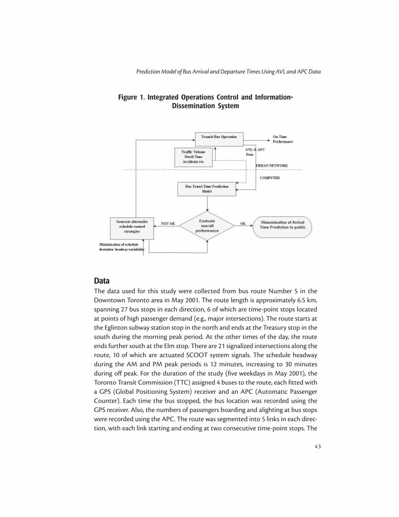
Prediction Model of Bus Arrival and Departure Times Using AVL and APC Data
4 3
Figure 1. Integrated Operations Control and Information-Dissemination System
DataThe data used for this study were collected from bus route Number 5 in theDowntown Toronto area in May 2001. The route length is approximately 6.5 km,spanning 27 bus stops in each direction, 6 of which are time-point stops locatedat points of high passenger demand (e.g., major intersections). The route starts atthe Eglinton subway station stop in the north and ends at the Treasury stop in thesouth during the morning peak period. At the other times of the day, the routeends further south at the Elm stop. There are 21 signalized intersections along theroute, 10 of which are actuated SCOOT system signals. The schedule headwayduring the AM and PM peak periods is 12 minutes, increasing to 30 minutesduring off peak. For the duration of the study (five weekdays in May 2001), theToronto Transit Commission (TTC) assigned 4 buses to the route, each fitted witha GPS (Global Positioning System) receiver and an APC (Automatic PassengerCounter). Each time the bus stopped, the bus location was recorded using theGPS receiver. Also, the numbers of passengers boarding and alighting at bus stopswere recorded using the APC. The route was segmented into 5 links in each direc-tion, with each link starting and ending at two consecutive time-point stops. The
Journal of Public Transportation, Vol. 7, No. 1, 2004
4 4
links range from 0.40 to 1.7 km in length, depending on the spacing between thetime-point stops, and may include 2 to 8 minor bus stops. This study focused onmodeling travel times along those links for the morning peak-hour bus opera-tion.
ApproachAs implied earlier, most of the models found in the literature (e.g., Kalaputapu andDemetsky 1995; Lin and Zeng 1999; Wall and Dailey 1999; Farhan et al. 2002) haveincluded bus dwell times along any link in the travel time of that link (i.e., link traveltime includes running plus dwell times). As such, these models cannot considerexplicitly the effect of late or early bus arrivals at bus stops on the dwell times atthose stops and vice versa. Ignoring such relationship yields these models insensi-tive to the effects of variations at upstream bus stops, such as demand surge, busholding strategy, and bus expressing strategy, etc., on downstream bus arrivalsand subsequent dwell times. The approach taken in this study addresses this issue.
Conceptual FrameworkThe link running time and bus dwell time are modeled separately in this study butin a consistent single modeling framework. It is assumed that real-time informa-tion on vehicle location, numbers of boarding and alighting passengers at busstops, and bus arrival and departure times is known from the AVL and APC sys-tems. The prediction modeling system consists of two separate algorithms, eachbased on the Kalman filter method. To predict the bus running time along aparticular link at instant k+1, the first algorithm, Link Running Time PredictionAlgorithm, makes use of the last three-day historical data of the bus link runningtime for the instant of prediction k+1, as well as the bus link running time for theprevious bus on the current day at the instant k. The study used data for theprevious three days only as this was deemed practical, given the limited historicaldata available for the study. Obviously, in real-world applications, the algorithmcan make use of longer ranges of historical data. The second algorithm, PassengerArrival Rate Prediction Algorithm, employs similar historical data of passenger ar-rival rate. To predict the dwell time at a particular stop, the predicted arrival rate issimply multiplied by the predicted headway (i.e., the actual arrival time of the lastbus minus the predicted arrival time of the next bus) and by the passenger board-ing time (assumed 2.5 seconds per passenger).

Prediction Model of Bus Arrival and Departure Times Using AVL and APC Data
4 5
Separating the bus dwell time prediction from bus running time prediction in thismodeling framework enhances the model’s ability to capture the effects of late-ness or earliness of bus arrivals at stops on the bus dwell time at those stops, andhence the bus departure from such stops. This is simply because bus dwell time ata stop is affected by the actual arrival time of the bus at that stop, particularly forhigh frequency transit routes where passengers are expected to arrive at a nearlyconstant rate (i.e., the later the bus, the longer the dwell time and vice versa). Inaddition, since the model treats dwell time separately, it is sensitive to stop-basedcontrol strategies such as bus holding and expressing.
In order to better understand the prediction-modeling framework, Figure 2 showsa schematic of a hypothetical transit route. The route is divided into a number oflinks between bus stops. When the transit bus n leaves stop i, the actual departuretime is known from the AVL system. At this instant, the Kalman filter predictionalgorithm for link running times will predict the next link running time RTn (i,i+1).Subsequently, the predicted arrival time of the bus at the downstream bus stopi+1 can be determined.
Figure 2. Schematic of a Bus Route with Several Stops
Assuming that bus n is currently at stop i
ATn
(i+1) = DT
n
(i) +RT
n (i,i+1) (1)
Where:
ATn (i+1)
is the predicted arrival time of bus n at stop i+1
RTn (i,i+1) is the predicted running time between i and i+1 from KalmanFilter prediction algorithm
DTn
(i)is the actual departure time of bus n from stop i

Journal of Public Transportation, Vol. 7, No. 1, 2004
4 6
This predicted arrival time ATn (i+1) is used to predict the dwell time for bus n atstop i+1 based on the passenger arrival rate and the average passenger boardingtime at stop i+1.
DWTn (i+1)
= 88888 (i+1)
* [ATn
(i+1) - AT
n-1
(i+1)] * DDDDDavg
(i+1)
(2)
Where:
DWTn (i+1) is the predicted dwell time for bus n at stop i+1
88888 (i+1)
represents the predicted passenger arrival rate at stop i+1 fromKalman filter prediction algorithm
ATn-1
(i+1)
is the actual arrival time of the previous bus n-1 at stop i+1
[ATn (i+1) - ATn-1 (i+1)] is the predicted headway for bus n at stop i+1
DDDDDavg (i+1) represents average passenger boarding time at stop i+1, assumedto be 2.5 seconds/passenger.
In equation (2), the assumption is that the boarding passengers at each bus stophave a significant effect on bus dwell time at that stop, compared with alightingpassengers. The time points used in this study, for which equation (2) applies, arelocated at high demand spots (i.e., subway station and major intersections) wherestop skipping because of no passenger demand is extremely rare. If stop skippingat a particular time point were frequent, equation (2) would need to be modifiedto address this problem.
Having the arrival time and dwell time for bus n at stop i+1 predicted, it is now easyto calculate the predicted departure time for bus n from stop i+1 by adding thepredicted arrival time to the predicted dwell time at stop i+1.
DTn (i+1)
= ATn (i+1)
+ DWTn
(i+1) (3)
Where:
DTn (i+1) is the predicted departure time for bus n from stop i+1

Prediction Model of Bus Arrival and Departure Times Using AVL and APC Data
4 7
This departure time prediction DTn (i+1) is a function of both arrival time predic-tion and dwell time prediction at stop i+1. Hence, the effect of any variations inbus operation (i.e., bus early or late) could be captured in this stop and will bereflected on all downstream bus stops.
Similarly, predictions of arrival times and departure times at all downstream stopscan be computed while the bus is still at stop i. This process is updated every timethe bus leaves or arrives at a new time-point stop.
Kalman-Filter Prediction AlgorithmsAs mentioned above, the prediction modeling system consists of two Kalmanflter algorithms. In general, the Kalman flter is a linear recursive predictive updatealgorithm used to estimate the parameters of a process model. Starting with initialestimates, the Kalman flter allows the parameters of the model to be predictedand adjusted with each new measurement. Its ability to combine the effects ofnoise of both the process and measurements, in addition to its easy computa-tional algorithms, has made it very popular in many research fields and applica-tions, particularly in the area of autonomous and assisted navigation (for furtherinformation on Kalman filters, see Maybeck 1979).
The main assumption used in developing the Kalman filters is that the patterns ofthe link running time and passenger arrival rate at stops are cyclic for a specificperiod of day. In other words, knowledge of the link travel time and number ofpassengers waiting for a specific bus in a certain period of time will allow one topredict these variables for the next bus during the same period, so long as condi-tions remain steady. When conditions change (e.g., demand surge at a stop and/or an incident occurred at a link), the model can update the effect of the newconditions on the predictions, so long as the new conditions persist for a suffi-cient length of time (at least one headway length).
The Kalman filter algorithm works conceptually as follows. The last three-dayhistorical data of actual running times along a particular link at the instant k+1plus the last running time observation at the instant k on the current day are usedto predict the bus running time at the instant k+1. Similarly, passenger arrival ratesof the previous three days at the instant k+1 plus the passenger arrival rate at theinstant k on the current day are used to predict the passenger arrival rate at theinstant k+1. The historical passenger arrival rate is obtained from the APC data asin this fashion: The number of on-passengers at a bus stop is divided by the mostrecent headway (i.e., the arrival time of the previous bus minus the arrival time of

Journal of Public Transportation, Vol. 7, No. 1, 2004
4 8
the current bus). Below are the equations used for the Kalman filter predictionalgorithms.
Link Running Time Prediction AlgorithmGenerally, a Kalman filter algorithm for bus link running time has the followingstructure (Reinhoudt and Velastin 1997):
(4)
a(k + 1) = 1 – g(k + 1) (5)
e(k +1) = VAR[datain] AAAAA g(k + 1) (6)
P(k + 1) = a(k+1) AAAAA art(k) + g(k+1) AAAAA art1(k + 1) (7)
where:
g equals the filter gain
a is the loop gain
e represents filter error
p equals prediction
art(k) is actual running time of the previous bus at instant (k)
art1(k+1) is actual running time of the previous day at instant (k+1)
VAR[data out] equals the prediction variance
VAR[data in
] is the last three days “art3(k+1), art2(k+1) and art1(k+1)”variance

Prediction Model of Bus Arrival and Departure Times Using AVL and APC Data
4 9
The input variance VAR[datain] is calculated at each instant k + 1 using the actualrunning time values for the last three days: art1 (k + 1), art2 (k + 1) and art3 (k + 1):
VAR[datain] = VAR[art1(k + 1),art2(k + 1),art3(k + 1)] (8)
where:
art1 (k+1) is the actual running time of the bus at instant (k+1) onthe previous day
art2
(k+1) is the actual running time of the bus at instant (k+1)two days ago
art3
(k+1) is the actual running time of the bus at instant (k+1)three days ago
The definition of the variance for a random variable is:
VAR[X] = E[(X – E[X])2] (9)
(10)
Now the variance can be calculated as shown in equation (14):
∆1 = [art1(k+1) – avg(art)]2 (11)
∆2 = [art2(k+1) – avg(art)]2 (12)
∆1 = [art
3(k+1) – avg(art)]2 (13)
(14)

Journal of Public Transportation, Vol. 7, No. 1, 2004
5 0
VAR[dataout] is based on the model prediction output and the correspondingfuture observation. Both pieces of data are not available, since the prediction isnot made yet and the future trip has not been made either. Ideally, VAR[data
out]
should be equal to VAR[datain] for good prediction performance (Maybeck 1979).Now, a new variance is introduced VAR[localdata]. It is equal to the variance of theinput and output data.
VAR[localdata
] = VAR[datain
] = VAR[dataout
] (15)
and equations (4) and (6) become:
(16)
e(k + 1) = VAR[localdata] AAAAA g(k + 1) (17)
Now it becomes easy to implement the actual Kalman filter algorithm to predictthe bus running times along the links. The order of applying the equations shouldbe (16), (5), (17), and (7).
Passenger Arrival Rate Prediction AlgorithmA Kalman filter algorithm was also developed to predict the passenger arrival rateusing data from the APC and AVL systems. At the prediction instant k+1, thehistorical passenger arrival rates (at instant k+1 of the previous three days andinstant k of the current day) at a particular stop are computed based on thenumber of corresponding boardings divided by the actual previous headway.Similar equations to those of the running time Kalman filter were developed andused to predict the passenger arrival rate at instant k+1.

Prediction Model of Bus Arrival and Departure Times Using AVL and APC Data
5 1
Model Performance EvaluationIn order to assess the predictive performance of the Kalman filter model, it iscompared with three previously developed models for the same route. They in-clude historical average model, regression model, and an artificial neural network(specifically, Time Lag Recurrent Network [TLRN]). A more detailed exposition ofthe models can be found elsewhere (Farhan et al. 2002). Similar to most modelsfound in the literature, the regression and TLRN models predict individual linktravel times, which include running plus dwell times. Another distinct feature ofthose models is their static nature, in that the model parameters are not updatedwith new available data. As mentioned earlier, the AVL and APC data for the studyroute were available for five consecutive days. The regression and TLRN modelswere developed using data of four days only, with the fifth day’s data held out fortesting.
Four testing datasets were used for the comparison; the first set includes the holdout data of the fifth day of observations, while the remaining three sets includeartificial data collected from three different bus operation scenarios representing:normal-condition bus operation, special-event scenario where there is a demandsurge on transit service, and lane-closure scenario where one lane on a specific linkis blocked (e.g., due to an accident or construction work). In contrast to the holdout data and normal condition scenario, the lane closure and special event sce-narios represent atypical conditions. Because real-world data of such conditionsare hard to obtain, the VISSIM traffic microsimulation software was used to simu-late these scenarios. Simulation of the entire corridor, calibration results and simu-lation of the scenarios are described elsewhere (Farhan 2002). After each simula-tion run, all the necessary data required for model testing was extracted and ana-lyzed. Three prediction error measurements were computed for all developedmodels to test the model performance (Okutani and Stephanedes 1984). Theseerror indices include:
Mean relative error (gggggmean), which indicates the expected error as a fraction of themeasurement
(18)

Journal of Public Transportation, Vol. 7, No. 1, 2004
5 2
Root squared relative error (gggggrs), which captures large prediction errors
(19)
Maximum relative error (gggggmax), which captures the maximum prediction error
(20)
where:
N is the number of samples (here N=50) X true(t) = measured valueat time t
X pred (t) is the predicted value at time t.
Table 1. Relative Error Results of the Prediction ModelsUsing “Hold Out” Data

Prediction Model of Bus Arrival and Departure Times Using AVL and APC Data
5 3
Table 1 shows the three error measures gmean, grs, gmax for the hold out dataset,while Figure 3 (a, b, c) summarize the performance of the three prediction modelsfor each simulated scenario. Obviously, the lower the error, the better the modelperformance.
Figure 3. Relative Error Results of the Prediction ModelsUsing Artificial Data (a, b, c)
(a)
Normal Condition Scenario
Total Historical Avg Regression Neural Network Kalman Filterε mean 0.330 0.124 0.111 0.097ε rs 0.305 0.132 0.120 0.124ε max 1.253 0.695 0.584 0.299

Journal of Public Transportation, Vol. 7, No. 1, 2004
5 4
(c)
Special Event Scenario
Total Historical Avg Regression Neural Network Kalman Filterε mean 0.679 0.218 0.220 0.123ε rs 0.685 0.240 0.239 0.127ε max 1.411 0.998 0.830 0.349
(b)
Lane Closure Scenario
Total Historical Avg Regression Neural Network Kalman Filterε mean 0.881 0.392 0.316 0.232ε rs 0.933 0.428 0.442 0.349ε max 2.362 1.324 0.830 0.547

Prediction Model of Bus Arrival and Departure Times Using AVL and APC Data
5 5
DiscussionThe results summarized in Table 1 show that for all links, the Kalman flter modelprovides the minimum value for the error measures gggggmean, gggggrs, gggggmax, pointing to thefact that its performance was the best compared with the other prediction mod-els, except for link #4 where the regression and TLRN models perform slightlybetter than the Kalman flter model.
Table 1 and Figure 3 (a, b, c) shows there is no significant difference in the perfor-mance of the regression and artificial neural network models for the three differ-ent scenarios. Both models give similar performance results for each scenario;their accuracy performance decreased for the special event and lane closure sce-narios. But in general, the artificial neural network model always gives lower valuesfor the relative error indices.
The Kalman filter model shows the best prediction performance in the simulatedscenarios. In particular, it showed superior performance to the other models inthe special event and lane closure scenarios. These results show the superior per-formance of the Kalman filter model compared with other prediction models interms of relative error. The results also demonstrate how this model can capturedynamic changes due to different bus operation characteristics.
In addition to its highly accurate performance in dynamic environments, themodel has the advantage of capturing the effects of control strategies, such asholding and expressing at upstream bus stops. For example, if the bus is currentlyat a time point where it will be held for an additional one minute, the modelappropriately captures the effect of this extra time on the arrival time at the nextbus stop and the dwell time at the next stop (which is function of number ofpassengers waiting at that bus stop when the bus is predicted to arrive) and soforth for the prediction of arrival and dwell times at subsequent stops.
User-Interactive Decision Support SystemThe developed arrival/departure time prediction model was used to build a DSS(Decision Support System) for dynamic control. This system simply uses the time-table of the time points to develop a time profile for each scheduled trip along theroute (i.e., schedule travel time profile; see Figure 4), which is done for each bus atthe start of its journey. Another prediction travel time profile is constructed usingthe Kalman filter prediction model. The prediction travel time profile is updateddynamically every time the bus arrives and departs from a time point.

Journal of Public Transportation, Vol. 7, No. 1, 2004
5 6
By using these two travel-time profiles, we are able to predict if the bus is runningearly or late at each time point. This is shown in Figure 4 as ∆. A positive value of ∆means that the prediction profile is currently lying above the scheduled one (buswill reach the downstream time points late), while a negative value of ∆ occurswhen the prediction profile lies below the schedule (bus will be ahead of sched-ule). In these cases, implementation of a corrective proactive control strategy isrequired to prevent expected schedule deviation downstream. A value of 0 refersto the compliance of the bus to the schedule. The value of ∆ is the key factor fordeciding what type of control strategy to implement. If ∆ is positive, an expressingtype of control is required to be applied, while a negative value of ∆ indicatesimplementation of some type of holding strategy.
Figure 4. Schedule Travel Time Profile

Prediction Model of Bus Arrival and Departure Times Using AVL and APC Data
5 7
System Design and ArchitectureThe proposed system, shown in Figure 5, is an interactive program developedusing the Visual Basic programming language. This program effectively utilizesAVL and APC data for dynamic bus arrival/departure information and perfor-mance analysis at downstream bus stops for the purpose of applying real-time,proactive control strategies.
Figure 5. Illustration of the Interactive Decision Support System

Journal of Public Transportation, Vol. 7, No. 1, 2004
5 8
The program records the dynamic actual location and time of the transit vehiclewhen it arrives and leaves all time points along the transit route based on the AVLdata. Also, it records the number of passengers alighting and departing the bus ateach stop. Real time AVL and APC information is transferred instantly from theserver to the program. For a specific bus trip, at the departure instant of bus fromthe terminal station, the prediction algorithms will automatically be activated topredict arrival and departure times of the bus at all downstream time points(prediction profile). At the same time, the associated bus departure schedule forall time points along the route is also displayed (schedule profile). The differencebetween the predicted and the schedule departure (∆ information) is automati-cally computed for all time points. If the value of the predicted bus time deviation∆ is within an accepted range (e.g., 0 to 2 minutes), the predicted departure timesare within the schedule, and no control strategies are required to be implemented.In such a case, the program will display black font color with white backgroundfor ∆ value labels. On the other hand, when ∆ values are more than 2 minutes (i.e.,bus expected to arrive/depart late at downstream time points), the font color willdisplay red. The transit controller can interact with the program to assess theeffect of bus expressing at one or more downstream time points (by setting dwelltimes at 0 for such time points) so as to as reduce predicted deviations. If the ∆value is less than 0 (i.e., bus expected to be ahead of schedule), then the ∆ valuelabel background is displayed red and the font color is black. The controller canassess the effect of bus holding at one or more downstream time points (byincreasing the dwell times at those time points). The interaction with the programcould be done by setting values under the “arrive” or “depart” button of theselected current/downstream time point (as shown on the left hand side of Figure5), then clicking on the corresponding “arrive” or “depart” button to updatemodel predictions.
The prediction algorithms of the system will be dynamically updated based on theAVL and APC data. As soon as the bus arrives or departs a new time point, newarrival and departure time predictions and new ∆ values for the remaining timepoints downstream will be processed.
At the end of each trip, the system records the observed AVL arrival and departuretimes as well as the real APC data regarding the number of passenger boardingsand alightings at each bus stop. These data are used to update the system histori-cal database (link running time and passenger arrival rate at time points) to beused for the Kalman filter predictions of future trips.

Prediction Model of Bus Arrival and Departure Times Using AVL and APC Data
5 9
In addition, the system computes the on-time route performance for each trip bycomparing the actual bus arrival/departure with the schedule arrival/departuretimes for all time points. The average on-time performance is automatically calcu-lated and displayed on the screen for all trips. This feature provides the transitmanagement with an easy tool to evaluate the route level of service in terms of on-time performance. The information and analysis provided by this system couldpossibly be used for updating and adjusting schedules.
ConclusionAn innovative model was developed for dynamic bus arrival and departure timeprediction. The model is based on two Kalman filter algorithms for the predictionof running times and dwell times alternately in an integrated framework. As such,the model can capture the interaction between the two variables (i.e., the effect ofone on the other). The model was shown to outperform other traditional models(regression and neural network models) in terms of predictive ability when testedon “hold out” real-world data. More importantly, the superiority of the modelwas even more prominent when tested on two simulated scenarios representingpassenger demand surge (e.g., because of a special event) and lane closure (e.g.,because of an incident). This is primarily due to continuous updating of the modelparameters based on dynamic real-time data, as opposed to traditional modelswhich are typically calibrated using historical data, with infrequent recalibration ofthe model, if any.
Because dwell time is predicted separately and its effect on bus arrival times atdownstream stops is accounted for, the model can be used for assessing transitstop-based dynamic control actions (e.g., bus holding, bus expressing). A user-interactive DSS was developed to provide continuous information on the ex-pected arrival and departure times of buses at downstream stops; hence the ex-pected deviations from schedule. The system enables the user to assess in real timetransit stop-based control actions to avoid such deviations before their occur-rence, allowing for proactive control, as opposed to the traditional reactive con-trol which attempts to recover the schedule after deviations occur.
The model developed here was based on data from one bus route in downtownToronto. However, the same modeling approach is applicable to other medium-to low-frequency routes where schedule control and dissemination of expectedarrival times are relevant.

Journal of Public Transportation, Vol. 7, No. 1, 2004
6 0
Further work can improve the model developed here in several ways. For example,better representative distributions of passenger arrivals at bus stops could beattempted instead of the implied uniform distribution assumed here. Also, fur-ther investigation is required to develop predictive models for overlapping routesthat serve the same bus stops. In such cases, a special consideration should begiven to dwell time prediction. Finally, the assessment of the model developedhere would be greatly enhanced if tested in the field under both normal andatypical conditions.
Acknowledgments
The research reported in this article was funded by the Geomatics for InformedDecisions (GEOIDE) network, a Network of Centres of Excellence funded by theGovernment of Canada.
References
Farhan, A., A. Shalaby, and T. Sayed. 2002. Bus travel time prediction using GPS andAPC. ASCE 7th International Conference on Applications of Advanced Tech-nology in Transportation, Cambridge, Massachusetts (August).
Farhan, Ali. Bus arrival time prediction for dynamic operations control and pas-senger information systems. 2002. Unpublished Thesis of Masters of AppliedScience, Department of Civil Engineering, University of Toronto.
Kalaputapu, Ravi, and Michael J. Demetsky. 1995. Modeling schedule deviations ofbuses using Automatic Vehicle Location data and artificial neural networks.Transportation Research Record 1497, 44-52.
Lin, Wei-Hua, and Jian Zeng. 1999. Experimental study of real-time bus arrival timeprediction with GPS data. Transportation Research Record 1666, 101-109.
Maybeck, Peter S. 1979. Stochastic models, estimation and control. Vol. 1, Aca-demic Press.
Okutani, Iwao, and Yorgos J. Stephanedes. 1984. Dynamic prediction of trafficvolume through Kalman filter. Transportation Research Board 18B(1), 1-11.

Prediction Model of Bus Arrival and Departure Times Using AVL and APC Data
6 1
Reinhoudt, Edwin M., and S. A. Velastin. 1997. A dynamic predicting algorithm forestimating bus arrival time. 8th IFAC/IFIP/IFORS Symposium, Vol. 3.,1295-8.Crete, Greece (June 16-18).
Wall, Z., and D. J. Dailey. 1999. An algorithm for predicting the arrival time of masstransit vehicle using Automatic Vehicle Location data. Transportation Re-search Board Paper No. 990870. 78th Annual Meeting, Washington, D.C.
About the Authors
AMER SHALABY ([email protected]) received his master and Ph.D. degrees fromthe Department of Civil Engineering, University of Toronto (U of T) in 1991 and1997, respectively. He was a postdoctoral fellow at U of T’s Joint Program of Trans-portation in 1996-1997 and an NSERC Industrial Research Fellow at IBI Group in1997-1998. Between 1998 and 2000, he was an assistant professor at RyersonUniversity, where he also directed the Vehicle Safety Research Centre. Since January2001, Dr. Shalaby has been an assistant professor at the University of Toronto. Heis specialized in the area of Intelligent Transportation Systems, with emphasis ontransit applications. His research interests also include transportation system plan-ning and road safety.
ALI FARHAN ([email protected]) received his master’s degree from the De-partment of Civil Engineering, University of Toronto (U of T) in 2002. Subse-quently, he worked as a research associate at the Joint Program in Transportationat the University of Toronto, then as a transportation engineer with MaricopaAssociation of Governments, Phoenix, Arizona. Currently, Mr. Farhan works forthe City of Calgary.

Journal of Public Transportation, Vol. 7, No. 1, 2004
6 2

Transit Network Optimization—Minimizing Transfers and Optimizing Route Directness
6 3
Transit Network Optimization –Minimizing Transfers and
Optimizing Route Directness
Fang Zhao, Florida International UniversityIke Ubaka, Florida Department of Transportation
AbstractAbstractAbstractAbstractAbstract
This paper presents a mathematical methodology for transit route network optimi-zation. The goal is to provide an effective computational tool for the optimization oflarge-scale transit route networks. The objectives are to minimize transfers andoptimize route directness while maximizing service coverage. The formulation of themethodology consists of three parts: (1) representation of transit route networksolution space; (2) representation of transit route and network constraints; and (3)solution search schemes. The methodology has been implemented as a computerprogram and has been tested using previously published results. Results of these testsand results from the application of the methodology to a large-scale realistic net-work optimization problem in Miami-Dade County, Florida are presented.
IntroductionTransit route network (TRN) design is an important component in the transitplanning process, which also includes transit network schedule (TNS) design. ATRN optimization process attempts to find the route network structure withoptimal transfer, route directness, and ridership coverage. Unfortunately, TRNdesign optimization processes suffer from combinatorial intractability, and thusfar for practical transit network problems of large scales, TRN designs seem to be
Journal of Public Transportation, Vol. 7, No. 1, 2004
6 4
limited to the use of various heuristic approaches where the solution searchschemes are based on a collection of design guidelines, criteria established frompast experiences, and cost and feasibility constraints. A systematic mathematicalmethodology applicable to large-scale transit networks for TRN optimizationdesign seems to be missing.
The quality of a TRN may be evaluated in terms of a number of network param-eters, such as route directness, service coverage, network efficiency, and number oftransfers required. Route directness refers to the difference between the triplengths,1 if the trip is to be made by transit or by a car following the shortest path.Service coverage refers to the percentage of the total estimated demand (mea-sured by transit trips) that potentially can be satisfied by the transit services basedon a given transit route network. In this study, if the origin and destination of apotential transit trip are within walking distance of a transit stop and are con-nected by transit routes, the trip is considered served by the network or “covered.”Network efficiency reflects the cost of providing transit services within a givennetwork, other things being equal. Transfers are a result of the inability of a givennetwork to provide direct service between all pairs of origins and destinations.Stern (1996) conducted a survey of various transit agencies in the United States,and about 58% of the respondents believed that transit riders were only willing totransfer once per trip. This suggests that the ridership of a transit system may beincreased by merely reducing required transfers through the optimization of aTRN configuration. In addition to increasing ridership, an improved TRN con-figuration may also reduce transit operating cost and allow more services to beprovided.
For transit systems with small bus route networks, a seasoned planner may be ableto obtain near optimal bus route network results based on personal knowledge,experience, and certain guidelines. For large transit systems, intuition, experiences,and simple guidelines may be insufficient to produce even near-optimal transitroute network configurations, due to the problem complexity. Therefore, sys-tematic methodologies are needed to obtain better TRN configurations. Thispaper presents a methodology for TRN structure optimization based on a math-ematical approach with the objectives of minimizing transfers, optimizing routedirectness, and maximizing service coverage (Zhao 2003). The methodology hasbeen implemented as a computer program and has been tested using previouslypublished results and a large-scale realistic network optimization problem inMiami, Florida.

Transit Network Optimization—Minimizing Transfers and Optimizing Route Directness
6 5
Formulation of A TRN Optimization ProblemA TRN optimization problem may be stated as the determination of a set oftransit routes, given a transit demand distribution in a transit service area andsubject to a set of feasibility constraints, to achieve objectives that optimize theoverall quality of a TRN. Mathematically, a typical network optimization processmay be stated as: optimize an objective function f(x,y,O) x X and y Y, sub-ject to certain constraints, where
x is a real vector, y is an integer vector (or a set of
vectors), and O is a matrix defined on the network’s node set. X is a space of realvectors, and Y is a set of integer vectors
Y = Y
where N is an integer set. A combinatorial optimization problem is a special case ofinteger optimization problems and refers to an integer optimization problemwhere the integer vector’s component set in vector y(i
1, i
2,…, i
s) is an ordered
subset of a larger integer base set N{n1, n2,…, nn}, i.e., (i1, i2,…, is) d N{n1, n2, …, nn}and n > s (in this paper, an ordered set is enclosed in parentheses while an unor-dered set is enclosed in brackets). TRN design is a typical combinatorial optimiza-tion problem, where the base set N{n1, n2,…, nn} is the set of all street nodes suitableto serve as transit stops, and the combinatorial set P
N is the set of all paths in the
street network suitable for transit vehicle operations. The matrix O = O(oij) repre-sents the transit demand at street nodes and is the OD matrix as oij represents thenumber of transit trips between street node n
i and n
j. This study deals with fixed
transit demand problems. O is assumed to be constant, representing transit de-mand for a given period of time of day, and does not change with transit supply. Itshould be recognized that, in reality, transit demand may depend on transit sup-ply, thus TRN optimization ideally should be carried out in an iterative manner ina cycle of demand estimation and route network design. A transit route may berepresented by an integer vector r (i
1, i
2,…, i
s) with its component set (i
1, i
2,…, i
s)
representing the sequence of a transit route’s stops. A transit route network con-sisting of l routes may be represented by a set of integer vectors,
y i1, i
2, ,i
s i
j N, j = 1, 2, , s

Journal of Public Transportation, Vol. 7, No. 1, 2004
6 6
T(l) = T(l){ r1, r2, …, rl }, rj = r (nj1, nj2, …, njs(j)), (j = 1, 2, …, l) (1)
where s(j) is the number of transit stops on transit route rj. •A transit route vectoris a member of the combinatorial space P
N , and a transit route network is a subset
of PN. Based on the above definitions and notations, a fixed demand TRN designoptimization problem may be stated as follows:
Maximize/minimize:
f(x, T(1), O) x X and T(1) d PN (2)
Subject to:
pi (x, T(l)) = 0, (i = 1, 2, …, ip ) and qi (x, T(l)) < 0, (i = 1, 2, …, iq) (3)
where the real vector x represents any continuous variables in the optimizationprocess, O is the OD matrix, and expressions in (3) represent various constraints ina TRN design process. Solving the TRN optimization problem, defined above,involves the search for an optimal set of feasible transit routes with unknowntopology/geometry. It is difficult to solve problems with a large number of integervariables, since the associated solution procedure involves discrete optimization,which usually requires the search for optimal solutions from an intractable searchspace (Garey and Johnson 1979).
Literature on TRN OptimizationA great deal of research has been conducted in the area of transit network optimi-zation. The methods in the literature may be roughly grouped into two catego-ries: mathematical approaches and heuristic approaches. However, there are noclear boundaries between these approaches. We consider an approach to be math-ematical if the problem is formulated as an optimization problem over a relativelycomplete solution search space. Generic solution search methods are then em-ployed to obtain solutions. Examples of such algorithms include various greedytype algorithms, hill climbing algorithms, simulated annealing approaches, etc.References and descriptions of various mathematical search algorithms may befound (e.g., Bertsekas 1998). We consider an approach to be heuristic if domainspecific heuristics, guidelines, or criteria are first introduced to establish a solutionstrategy framework. Mathematical programming or other techniques are thenemployed to obtain the best results. The main difference between these two ap-proaches is that the mathematical approach formulates a problem on a solutionspace with certain completeness that, theoretically, should include optimal solu-

Transit Network Optimization—Minimizing Transfers and Optimizing Route Directness
6 7
tions. In contrast, the heuristic approach formulates a problem directly on solu-tion sub-spaces defined based on domain specified heuristic guidelines.
Table 1 provides the main features of some of the approaches reported in theliterature, where MATH represents mathematical optimization, and H&M (heu-ristic and mathematical) means that the author(s) established a solution based ona heuristic framework, but employed certain mathematical optimization meth-ods at some solution stages. Most of the studies introduced some heuristics orcertain simplifying assumptions to limit the solution search space or to reduceoptimization objectives to a particular network structure or a few design param-eters, e.g., route spacing, route length, stop spacing, bus size, or service frequency.(Detailed information and reviews of various mathematical optimization ap-proaches may be found in Zhao 2003, among others.)
The advantage of heuristic approaches is that they are always able to providefeasible solutions to problems of any size while the main disadvantage is that theirresults are almost certainly do not provide global or even local optimal solutions.This may be because heuristic search schemes are usually ad hoc procedures basedon computer simulations of human design processes guided by heuristic rules.The corresponding search spaces are usually not clearly defined and search resultsare likely to be biased toward existing systems or any systems on which the set ofdesign heuristics are based.
Table 1. Main Features of Some Approaches Usedin Transit Network Design

Journal of Public Transportation, Vol. 7, No. 1, 2004
6 8
Compared with other methods in transit network design, mathematical ap-proaches usually have more rigorous problem statements. A major disadvantageof mathematical approaches in TRN design is the computational intractabilitydue to the need to search for optimal solutions in a large search space made up ofall possible solutions. The resultant mathematical optimization systems derivedfrom realistic combinatorial TRN problems are usually NP-hard, which refers toproblems for which the number of elementary numerical operations is not likelyto be expressed or bounded by a function of polynomial form (Garey and Johnson1979). For this reason, existing mathematical optimization solution approachesto TRN problems are usually applied to relatively small and idealized networks forsmall urban areas or medium-sized urban areas with coarse networks. The routenetwork structures may also be limited to certain particular configurations.
Solution MethodologyMethodology was developed based on the following considerations: (a) themethod should be generally applicable to the design and optimization of a widerange of TRN problems in practice; (b) the solution method should be as genericas possible and should not favor particular transit network configurations; and(c) solutions obtained from this method should give fairly good results in a rea-sonable amount of time, as permitted by the current computer power affordableto most transit agencies. Reliability of results should improve as the computerresource or power increases, and should approach the global optimum whenthere is no computer resource limitation.
Representation of Transit Service Area, Routes, and Route NetworkA transit service area is represented by a street network, which consists of a set ofstreet nodes that are connected to each other by a set of street segments. A streetsegment, a(n1, n2), may be defined by its two end nodes n1 and n2. In a directednetwork, segments a(n
1, n
2) and a(n
2, n
1) may be different as in the case of one-way
streets or when travel impedance on the same link is different in the two oppositedirections. In this study, only undirected network is considered (i.e., a(n1, n2) anda(n
2, n
1) are considered the same), but the methodology can be easily extended to
directed networks. It is also assumed that the street network is connected; thus,any two nodes in the street network are connected by at lease one path.
The following is the mathematical representation of a street network. Denote N(n)
= N(n){n1, n2, …, nn} as the set of n street nodes in a transit service area, then a streetnetwork consisting of m street segments may be written as A(m) = {a1, a2, … am},

Transit Network Optimization—Minimizing Transfers and Optimizing Route Directness
6 9
where ai = ai(ni1,ni2) and ni1, ni2 N(n) (i = 1, 2, …, m). A path/route between any two
nodes is defined as a sequence of non-reoccurring nodes, or p = p(n1, n2, …, nk),and there is one street segment, i.e., a(n
j, n
j+1) A(m) (j = 1, 2, …, k-1), that connects
any two neighboring nodes. A street network may also be represented throughan adjacency list of street nodes. For a given node, called the master node of thelist, its associated nodal adjacency list consists of all the neighboring nodes thatcan be connected to the master node with one street segment. The set of all nodaladjacency lists of a street network may be expressed as
L(k) = L(k){k1, k
2, …, k
m(k)}, k=1, 2,..., n (4)
where:
L(k) is the nodal adjacency list of the street node k
kj is the street node number of the jth neighboring node in the list
m(k) is the number of nodes in the list
The TRN T(l) in (2) may also be expressed as a TRN matrix.
T = T [tij], t
ij = (5)
In this study, for the purpose of representation uniqueness, it is assumed that thetransit route stop set and the corresponding street node subset are the same.
Representation of Search Spaces for Transit Routes and Route NetworkThe solution search spaces in this study are locally and iteratively defined, and thesize of a local search space may be flexible based on available computing resources.A local path space consists of three components: (1) a master path; (2) a key-noderepresentation of the master path; and (3) a set of paths that are in the neighbor-hood of the master path. A master path is a path from which a local path space willbe generated. Key nodes are a set of nodes on a master path selected to definedpaths in the local path space. A local path space is derived from the local nodespaces of the key nodes on the master path. An ith order local node space, denotedas N(i)(k), of a master node k is defined as the set of nodes that can be connectedto the master node with i or fewer street segments. The order of a local node spaceprovides a measurement of the degree of localization. Figure 1 illustrates a three-key-node (nodes n1, n2, and n3) representation of a master path (solid line) and the
91, if node j is on route i, i=1,2,...,l0, if node j is not on route i, j=1,2,...,n

Journal of Public Transportation, Vol. 7, No. 1, 2004
7 0
three first order local node spaces, N(1)(n1) = {n1, n11, n12, n13, n14}, N(1)(n2)= {n2, n21, n22, n23, n24}, and N(1)(n3) = {n3, n31, n32, n33, n34}.
Denote the (i-1)th order local node space of a master node k as N(i-1)(k) = •{k1, k2, …,k
q(k)}, where q(k) is the number of nodes in this local node space, then
N(i)(k) = {k1, k2, ..., kq(k)} c L(k1) c L(k2) c ... c L(kq(k)) (6)
where L (kj) is the nodal adjacency list of node kj. A local node space is a subspaceof the street node space N
(i) (k) f N(n). As the order i increases, it will approach to
the original street node space N(n). The procedure to generate a local path spacefrom a master path has three steps: (1) Select s key-nodes from the node set of themaster path p = p(n
1, n
2, …, n
r), i.e., {m
1, m
2, … , m
s} f {n
1, n
2, …, n
r};
(2) Generate a sequence of local node spaces from these key-nodes,(N(i)(m1), N(i)(m2),...,N(i)(ms)); and (3) Define the local path space as the set ofpaths consisting of piecewise shortest path segments that start from nodes in thefirst local node space N(i)(m1), sequentially pass the nodes in each of the interme-diate local node space N(i)(mj) (j = 2, 3, …, s-1), and end at nodes in the last localnode space N
(i)(m
s). The shortest path segments used to connect nodes in neigh-
boring local node spaces are from a k-level shortest path space PS(k) that consists of
all the first k shortest paths between any two nodes in the street node space N(n).(References on algorithms of finding a k-level shortest path space may be found inZhao 2003.) The resultant path space, denoted as, P(i)
(k) (p(s)), will be referred to asthe local path space based on the s-nodes representation of the master path p, orsimply the local path space of path p.

Transit Network Optimization—Minimizing Transfers and Optimizing Route Directness
7 1
The local network search spaces of a transit network T(l) = {r1, r2, …, rl} is defined as
(7)
where is a local path space of sj-node representation for master pathrj. It may be seen that as the two numbers i and k increase, a local path space of anymaster path will approach to the combinatorial path space P
N.
will be the path search space of the corresponding transit route rj. Ingeneral, routes derived from smaller numbers of key nodes will result in betterroute directness and smaller local path search space, but their flexibility is alsolimited. Routes with larger numbers of key nodes are relatively more flexible toreach more neighboring nodes, thus may cover more trips. However, this will alsoresult in larger local path search spaces, requiring more computing resources.
Integer Constraints for Transit Route NetworkInteger constraints in this study include the following: (a) fixed route constraintsprescribing fixed guideway lines or bus routes that are specified by transit plannersto meet certain planning goals, which will remain unchanged during the optimi-zation process; (b) constraints prescribing starting, ending, or in-between areasthrough which transit routes must pass, which may include major activity centersor transfer points; (c) route length constraints for individual transit lines or for theentire system; and (d) constraints on the number of transit stops on individualroutes.
Route Directness ConstraintsRoute directness used in this study is defined as follows:
(8)
where:
s is the number of nodes on route r = r(n1, n2, …, ns)
dij
(r) is the distance between nodes ni and n
j measured along the transit
route

Journal of Public Transportation, Vol. 7, No. 1, 2004
7 2
dij(S) is the shortest network distance between nodes ni and nj
wij are weighting factors
For geometry based route directness, wij = wijG ≡ 2/(s2 - s), and for ridership based
route directness,
where oij and o
ji are coefficients of the OD matrix. The geometry based route
directness, denoted as dG(r), reflects the average ratio of the two travel distances,d
ij(r) and d
ij(S), between each node pair on route r. A value of dG(r) = 1 indicates that,
on average, transit vehicles on route r travel along the shortest paths betweenroute stops. The ridership based route directness, dR(r), represents the averageratio of the distance a person travels between OD points along transit route r tothe distance traveled along the shortest path. A value of dR(r) = 1 indicates that, onaverage, passengers on transit route r travel along the shortest paths between ODpoints. Route directness constraints used in this study may be expressed as
or (i =1, 2,…,l), where drG and dr
R are the two travel di-rectness constraint parameters. In general, smaller dr
G and drR imply better ser-
vices, but may result in higher transit operating cost. Large drG and d
rR mean that
some potential transit riders may be turned away and that existing transit ridersmay be forced to look for other alternatives, thus leading to loss of ridership and,eventually, higher operation cost.
Network Directness ConstraintsTransit network directness has a physical meaning similar to that of the routedirectness, except that the directness measurement is based on geometry or rider-ship characteristics of the entire route network, instead of individual transit routes.
Out-of-Direction (OOD) ConstraintsThe OOD constraint used in this study is derived from the formulation given byWelch et al. (1991). Denote d
ij(O)(r) as the OOD impact index for travel between
nodes i and j on transit route r, then
dij
(O)(r) = rij
(1)(r)[lij(r)-d
ij]/r
ij(2)(r)
wij
= wijR ≡
Transit Network Optimization—Minimizing Transfers and Optimizing Route Directness
7 3
where:
rij(1)(r) is the through ridership, or the number of trips on route r that
pass through nodes i and j without boarding or alighting inbetween
rij
(2)(r) is the OOD ridership, which is the number of trips on route rthat involve either boarding or alighting or both at nodes be-tween nodes i and j
lij(r) is the distance between nodes i and j along route r
dij is the distance along the shortest path between these two nodesin the street network
dij
(O)(r) represents the extra travel distance that incurs to each throughpassenger in order to serve an OOD passenger.
Optimization Objective FunctionsObjective functions considered in this study are various trip coverage functions ortheir combinations. The goal is to obtain a TRN structure with minimum trans-fers, while optimizing service coverage. If a trip between an OD pair requires notransfers, the trip is called a zero-transfer trip, while a trip between an OD pair thatrequires k or fewer transfers will be called a k-or-less transfer trip. A k-or-less trans-fer trip coverage function, or simply a k-or-less transfer function, is defined as thetotal number of OD trips that can be accomplished with k or fewer transfers in atransit network service area. The following is a description of various transfercoverage functions used in this study. Denote f
k as a k-or-less transfer function,
then
, k = 0, 1, 2, (9)
where
T is the TRN matrix defined in (5)
O is the OD matrix
h is a step function that has the property:
h(x) = 1 for x > 0, and h(x) = 0 for x < 0

Journal of Public Transportation, Vol. 7, No. 1, 2004
7 4
Coefficients α ij(k) in (9) are defined as α ij
(0) = , α ij(1) = ,
α ij(2) = , αkm = , and βββββkm = , where tki, tkj, and tmj
are coefficients of matrix T. It may be seen that calculation of transfer objectivefunction, f2, is computational intensive, compared with functions f0 and f1, due tothe great number of arithmetic operations involved to obtain all the requiredcoefficients.
The use of any of the transfer functions alone as the objective function may resultin the optimization of one TRN parameter at the cost of others. The following aretwo objective functions that combine multiple coverage functions, thus givingmore balanced results.
(10)
, (11)
where
α is a weighting coefficient to penalize uncovered trips during the optimi-zation process of the TRN system
fT
is the total number of trips in the transit network service area
The physical meaning of the objective function t2 is the average number of vehicleboardings that a transit rider has to make to accomplish an OD trip. The optimalvalue of t
2 is 1.0, indicating that all trips are zero-transfer trips. Uncovered trips (f
T
– f2) are penalized by α . The value of α needs to be determined by transit planners.For example, by setting α = 4, each of the uncovered trips is considered as fourvehicle boardings. In general, the larger the value of α , the greater relative impor-tance is given to service coverage. The physical meaning of t1 is similar to that of t2.
Algorithm 1—Basic Greedy Search MethodThe basic assumption of Basic Greedy Search (BGS) is that the demand distribu-tion in a TRN service area has certain continuity. In other words, nodes withcertain transit demands are probably close to nodes with similar demands. In suchcases, it will be more effective in searching for a better solution by evaluating pathsthat are near nodes or areas with higher trip distributions. (Detailed description ofvarious search algorithms used in this study can be found in Zhao 2003.) Assume

Transit Network Optimization—Minimizing Transfers and Optimizing Route Directness
7 5
that during a solution search process, an intermediate TRN result T(l) = {r1, r2, … rl}has been obtained. The solution search procedure for the next stage of BGS methodinvolves the following steps:
1. Select key nodes from route rj. For illustration, assume the three-noderepresentation of route rj is used (see Figure 1), which is denoted as rj
(3).
2. From the three key nodes n1, n
2, and n
3, generate three first order local
node spaces
N(1)
(n1) = {n
1, n
11, n
12, n
13, n
14}
N(1)(n2) = {n2, n21, n22, n23, n24}
N(1)(n3) = {n3, n31, n32, n33, n34}
There are five nodes in each of the three local node spaces.
3. Connect nodes in node spaces N(1)(n1) and N(1)(n3) with the shortestpaths in space P
S(1), to obtain 5 × 5 = 25 shortest path segments. These
shortest path segments are then extended with shortest paths to nodesin node space N(1)(n2) to obtain 25 × 5 = 125 paths. These 125 paths formthe local path space of route r
j, based on three-node representation
.
4. Replace route rj in the existing TRN T(l) with a path r
jk0 to obtain
T(l) = {r1, …, rj-1, rjk, rj+1, …, rl}, and perform function evaluation for k = 1,2, …, 125. If a better result is obtained, replace r
j with r
jk, and go to Step 1
to start a new search. If no better result is found from all the 125 paths rjk0
, go to Step 5.
5. Select the next route from the transit route network, e.g., route r(j+1)
andgo to Step 1 to start a new local search for route r(j+1).
6. The search process will be considered converged if no better results canbe found from the local path search spaces of all the individual routes.
Algorithm 2—Fast Hill Climb Search MethodConceptually, the Fast Hill Climb (FHC) method is similar to the deepest decentmethod in continuous research fields. First, l new solutions are formed by replac-ing one route at a time in the network, with the best route from its local searchspace. These l best routes from the local search spaces also make up a new solu-

Journal of Public Transportation, Vol. 7, No. 1, 2004
7 6
tion. These l + 1 solutions are compared and the best one is chosen as the currentsolution. Note that the computation process to obtain the l best routes is inde-pendent to each other, making it suitable for parallel computing.
Numerical ExperimentsThe first test experiment was based on a real network in Switzerland (Mandl 1979).This problem was also used by Shih and Mahmassani (1994) and Baaj andMahmassani (1991) as a benchmark problem to test their approaches to TRN andTNS design optimization. Mandl problem consisted of a street network of 15nodes with a total demand of 15,570 trips per day. For this particular problem, thelength of a street segment was defined in terms of in-vehicle travel time in minutes.In Table 2, the first row identifies the source of the solutions to the benchmarkproblem. The second row indicates solutions to the benchmark problem withdifferent numbers of routes, total route length, and/or search methods. The meth-ods used to obtain the results are indicated in the third row. For each solution, theunshaded column provides the statistics for the layout produced in the originalstudies, and the shaded column gives the statistics for the results produced fromthe FHC method developed in this study.
It may seem that the percentages of zero transfer trips were higher for all solutionsproduced in this study. Except for Mandl’s original results, all solutions provided100% trip coverage with zero or one (one-or-less) transfer involved in each trip.
The second experiment involved a large-scale TRN optimization problem basedon the service area of the Miami-Dade Transit Agency (MDTA), encompassing a
Figure 1. Three-Key-Node Representation of Transit Route

Transit Network Optimization—Minimizing Transfers and Optimizing Route Directness
7 7
region of about 300 square miles with a population of about 2.3 million. MDTA isranked the 16th largest transit agency in the United States. At the time of thisresearch, MDTA operated 83 transit routes, including a rail rapid transit system of22.5 route miles (Metrorail), a 4.5-mile downtown automated circulation system(Metromover), and 81 bus routes with about 4,500 transit stops. The street net-work used in this experiment consisted of 4,300 street segments and 2,804 streetnodes. In the optimization process, Metrorail and Metromover alignments werefixed and the longest and shortest bus routes were about 32 miles and 4 miles,respectively. The total length of the transit system was about 1,300 route miles,omitting some small loops at the ends of some routes or in shopping centers. TheOD matrix was generated from the 1999 validated Miami-Dade travel demandmodel, which provided the daily number of passenger trips between each pair oftraffic analysis zone centroids. These were manually distributed to the surround-ing street network nodes with considerations given to land use patterns andstreet network connectivity. The total demand was 161,944 daily transit trips. Allthe numerical results were obtained on a personal computer with a 2.8GHz CPUand 1GB RAM memory. Table 3 presents the results from the BGS and FHC meth-ods. There were two sets of results produced by each method, one based on aninitial guess network that was the existing route network and the other based ona program generated initial guess network. The constraints were that the total
Table 2. Comparison of Results from Different Methods

Journal of Public Transportation, Vol. 7, No. 1, 2004
7 8
route length of the network should not exceed that of the existing system bymore than 10%, and that the total number of transit lines remained the same asthe existing system. Two objective functions were used, one maximizing zero-transfer trips (f0) and the other maximizing one-or-less transfer trips (f1). Thevalues of the objective functions are given in the shaded cells.
Compared to the existing network, the FHC method with objective function f0
gave the best zero-transfer trip coverage, with an improvement of 85% (from14.28%to 26.41%), while the BGS search method yielded an improvement of 84%. Forobjective function f
1, the FHC method again gave the best one-or-less transfer trip
coverage, with a 48% improvement (from 55.13% to 81.57%). These improve-ments were achieved with a small increase of 5% in total network route mileage.Assuming most transit riders may be only willing to transfer once per trip (Stern1996), the one-or-less trip coverage shown in the fourth row would be the actualtotal trip coverage of the corresponding route networks. The remaining trip de-mand either required two or more transfers or were not satisfied.
Table 3. Comparison of Results with the Existing Network

Transit Network Optimization—Minimizing Transfers and Optimizing Route Directness
7 9
The number of covered trips per route mile shown in Table 3 was defined as
=
where
f2
was the number of trips accomplished with two-or-less transfers
lT was the total length of the TRN
As a network efficiency indicator, the best value was given by the BGSmethod with f1 as the objective function. The average transfers were defined as[f0 + 2(f1 - f0) + 3(f2 – f1)]/f2, which was the average number of boardings per transitrider who could complete a trip with two or fewer transfers. For the same objec-tive function, the FHC method produced slightly better results than the BGSmethod. It may be seen that the differences in results produced by the BGS andFHC search methods were insignificant, but the BGS method was significantlyfaster than the FHC method.
Table 4 presents results obtained from composite trip coverage functions t1 and t
2
described in (10) and (11), with the shaded cells indicating the objective functionvalues. The penalty a was set at 4 in both functions t1 and t2. It may be seen thatimprovements in various trip coverage functions were consistent instead of beingachieved at the cost of each other, as in the case of single trip coverage functionshown in Table 2. Overall, FHC produced slightly better results than those frommethod BGS, but at a higher computational cost.
ConclusionThe methodology developed from this work has a systematic mathematical state-ment of TRN problems, including the definition of various objective functions,solution search spaces, and constraint conditions commonly used in transit plan-ning fields, and a systematic scheme that flexibly defines solution search spacesbased on available computing resources and/or optimization problem sizes. Twolocal search schemes have been developed to obtain results for large-scale practicalproblems in a reasonable amount of time.
The feasibility of the proposed method has been tested through practical TRNoptimization problems of realistic sizes. Numerical results showed that the meth-odology developed in this work was capable of tackling large-scale transit networkdesign optimization problems. Further improvements may include development

Journal of Public Transportation, Vol. 7, No. 1, 2004
8 0
of TRN optimization methods that consider dynamic transit demand, demandand travel time in different time period of a day, and waiting and transfer penalties.
Acknowledgements
This research was sponsored by a grant from the Florida Department of Transpor-tation (FDOT). The opinions, findings, and conclusions expressed in this paperare those of the authors and not necessarily those of the FDOT. The authorswould like to thank the reviewers for their useful comments and suggestions.
Endnote1Depending on particular applications, length/distance may refer to either geo-metric length/distance or travel time.
Table 4. Comparison of Results with Existing Networks

Transit Network Optimization—Minimizing Transfers and Optimizing Route Directness
8 1
References
Baaj, M. H and H. S. Mahmassani. 1991. An AI-based approach for transitroute system planning and design. Journal of Advanced Transportation25(2): 187-210.
Bertsekas, D. P. 1998. Network optimization: continuous and discrete models.Belmont, MA: Athena Scientific.
Bookbinder, H. J. and A. Désilets. 1992. Transfer optimization in a transitnetwork.
Transportation Science (26)2: 106-118.
Chien, S., B., V. Dimitrijevic, and L. N. Spasovic. 2003. Optimization of busroute planning in urban commuter networks. Journal of Public Transpor-tation 6(1): 53-80.
Garey, M. R. and D. S. Johnson. 1979. Computers and intractability: A guide tothe theory of NP-completeness. Freeman, NY.
Mandl, C. E. 1979. Evaluation and optimization of urban public transporta-tion networks. European Journal of Operational Research (5): 396-404.
Shih, M. C. and H. S. Mahmassani. 1994. A design methodology for bus transitnetworks with coordinated operations. SWUTC/94/60016-1. Austin, TX:Center for Transportation, University of Texas at Austin.
Soehodo, S. and M. Koshi. 1999. Design of public transit network in urbanarea with elastic demand. Journal of Advanced Transportation 33(3): 335-369.
Stern, R. 1996. Passenger transfer system review. Synthesis of Transit Practice19, Transportation Research Board.
Welch, W., R. Chisholm, D. Schumacher, and S. Mundle. 1991. Methodologyfor evaluating out-of-direction bus route segments. Transportation Re-search Record 1308: 43-50.
Zhao, F. 2003. Optimization of transit network to minimize transfers. Drafttechnical report prepared for the Florida Department of Transportation.Miami: Lehman Center for Transportation Research, Florida InternationalUniversity.

Journal of Public Transportation, Vol. 7, No. 1, 2004
8 2
About the Authors
FANG ZHAO ([email protected]) received her Ph.D. in civil engineering from CarnegieMellon University. She teaches in the civil and environmental engineering depart-ment at Florida International University, and is associate professor and deputydirector of the Lehman Center for Transportation Research. Her main researchinterests include public transportation, travel demand modeling, geographic in-formation systems, and transportation data modeling. Dr. Zhao is a registeredprofessional engineer in the state of Florida and member of the TransportationResearch Board’s Transit Planning and Development Committee and New Tech-nologies and Systems Committee.
IKE UBAKA ([email protected]) is program manager for transit systems plan-ning at the Florida Department of Transportation, where he is responsible forstatewide transit systems planning. He has over 18 years of experience in transitplanning, including service with the Los Angeles County Metropolitan Transpor-tation Authority and the Orange County (California) Transportation Authority.Mr. Ubaka holds a master’s degree in urban and regional planning from UCLA anda master of administration degree from the University of California, Riverside. Heis a member of the American Institute of Certified Planners.

Vehicle Selection for BRT: Issues and Options
8 3
Vehicle Selection for BRT:Issues and Options
Samuel L. Zimmerman, DMJM+HARRISHerbert Levinson, Transportation Consultant
AbstractAbstractAbstractAbstractAbstract
Bus rapid transit (BRT) is a flexible, high performance rapid transit mode that com-bines facilities, equipment, service and intelligent transportation system (ITS) ele-ments into a permanently integrated system with a quality image and unique iden-tity. Vehicles are an extremely important component of BRT systems, because theynot only contribute significantly to BRT’s image and identity, but also play a strongrole in achieving measurable performance success.
Vehicle-related planning and design issues confront BRT planners in seven basic areas:
1. Capacity, External Dimensions
2. Internal Layout
3. Doors
4. Floor Height
5. Propulsion Systems
6. Vehicle Guidance
7. Aesthetics, Identity and Branding
This paper draws heavily on 26 case studies documented in TCRP Project A-23(Levinson, Zimmerman, et al. 2003). It also reflects experience from newer BRT

Journal of Public Transportation, Vol. 7, No. 1, 2004
8 4
systems and concludes with a series of general principles and guidelines for vehicledesign, selection, and use in BRT applications.
IntroductionBRT is a flexible, high performance, rapid transit mode that combines facility,equipment, service and ITS elements into a permanently integrated system with aquality image and unique identity. Its constituent elements include:
1. Running ways
2. Stops, stations and terminals
3. Vehicles
4. Services
5. Intelligent transportation systems
6. Fare collection
BRT must be planned as an integrated system ideally suited for the markets servedand the application’s physical environment. Having a quality image and a uniqueidentity distinct from the rest of the transit (i.e., local bus) system are also impor-tant BRT attributes.
Vehicles may be the most important element to user and non-user perceptions ofa BRT system’s quality. Vehicles also play a strong role in determining real perfor-mance in terms of speed, reliability, and cost. They are critical from the perspectiveof customers, the community as a whole, and the operating entity for a numberof reasons. First, vehicles have a strong effect on every aspect of measurable systemperformance.
• Propulsion systems impact revenue service times (thus, ridership and rev-enue), emissions (air pollutant and noise) and operating and maintenance(OM) costs.
• Seating, floor height, floor plan, and door configurations impact stopdwell times, hence, revenue service times and reliability.
• Physical size, aisle width, number of doors and their width and position,and seating numbers and configuration are important determinants ofBRT system capacity.

Vehicle Selection for BRT: Issues and Options
8 5
Second, since potential new transit customers as well as existing ones are exposedto BRT vehicles, their design impacts community and customer perceptions ofthe quality of the entire system. This perception is primarily visual and aesthetic,but it also relates to impacts such as noise and air emissions. Although not asimportant as time and cost in effecting mode choice, image and brand influencethe willingness of new customers to try BRT. This willingness to ride transit trans-lates into additional ridership, revenue and other related benefits, as do perfor-mance factors such as travel time and reliability.
One of the major products of TCRP Project A-23 (Levinson, Zimmerman, et al.2003) was the documentation of 26 case studies of BRT systems around the worldand the results of their assessments into a number of summary observations. Thesynthesis showed that the proliferation of BRT systems has accelerated the trendtoward more rubber-tired transit vehicle specialization, away from the one-size-fits-all (i.e., 40-foot [12 meter]) bus to perform all surface transit functions. Moreattention is being paid to the nature of the markets being served, service offered,and customer and non-customer perception of vehicle quality.
The discussion below provides planners with information that can help themmake better vehicle choices. It summarizes observations relating to BRT vehiclesfrom the case studies and other, more recent BRT applications, as well as the TCRPBRT guidelines. It is organized around seven basic themes:
1. Capacity, External Dimensions
2. Internal Layout
3. Doors
4. Floor Height
5. Propulsion Systems
6. Guidance
7. Aesthetics, Identity and Branding
Capacity and External DimensionsIn nearly all of the 26 case studies, demand was heavy, ranging up to 20,000 ormore passengers per hour. That utilization of high capacity (e.g., articulated buses)vehicles with a total capacity (standing + seated) of at least 65 places was essentialfor either system capacity and/or OM cost reasons. In the case of Los Angeles

Journal of Public Transportation, Vol. 7, No. 1, 2004
8 6
MTA’s MetroRapidBus and Boston MBTA’s Silver Line, BRT services were initiatedwith 40-foot (12 meter) vehicles, because long procurement times for larger (60-foot [18 meter]) vehicles would have delayed the start of service. Both the LA andBoston systems planned to have 60-foot vehicles. Eaarly on, demand had nearlyoutstripped the capacity of the 40-foot vehicles.
Less than one year after opening, some of the originally planned 60-foot (18 meter),low-floor (Neoplan CNG) vehicles are in operation on the Silver Line. In LA, 60-foot low-floor (NABI CNG) vehicles are on order after approximately three yearsof operation. Several BRT applications in South America and Europe, such asCuritiba and Sao Paulo, Brazil; Nancy, Nice and Caen, France; and Utrecht, Nether-lands, operate double articulated vehicles of up to 83 feet (25 meters) in length,having a capacity of over 120 total places (at North American loading standards).
Given the high demand nature of many BRT routes and services, transit operatorsare increasingly using large (over 40-foot) vehicles. The use of unusually large (forthe given community) rolling stock adds to BRT’s distinct identity, while the extracapacity is helpful for financial, service, and operational efficiencies.
Table 1 shows the external dimensions and capacities (computed for a standeedensity of 3 standees per square meter) for typical vehicles used in BRT applica-tions.
Table 1. Dimensions and Capacities of Typical U.S. and CanadianBRT Vehicles
Length Width Floor Height No. of No. of Maximum(Feet) (Inches) Door Seats Capacity*
Channels (including seated plusseats in standing
wheelchairtiedown
areas)
40 (12.2 m) 96-102 13-36 2-5 35-44 50-60(2.45-2.6m) (33-92 Cm)
45 (13.8 m) 96-102 13-36 2-5 35-52 60-70(2.45-2.6m) (33-92 Cm)
60 (18 m) 98-102 13-36 4-7 31-65 80-90(2.5-2.6m) (33-92 Cm)
80 (24 m) 98-102 13-36 7-9 40-70 110-130(2.5-2.6m) (33-92 Cm)
* Computed at Standee density of 3/mtr2

Vehicle Selection for BRT: Issues and Options
8 7
Interior ConfigurationThe interior configuration of BRT vehicles influences both passenger capacity andcomfort. As noted, the overall capacity of transit systems is influenced by a num-ber of vehicle-related factors, and the interior configuration is one of the moreimportant factors. Easy and rapid passenger boarding, alighting and internal cir-culation can minimize dwell times. BRT vehicle interior layouts usually includelarge standing/circulation areas around doors. These aid boarding, alighting, andcirculation and can also function as storage areas for baby carriages, bicycles, andwheelchairs, explicitly supporting the mobility needs of the entire community.
Aisle width also influences vehicle capacity. Most conventional low-floor vehicles,even those with a step-up to the rear portion of the vehicle, have a minimum aislewidth between the rear wheel wells (second and third axle on articulated vehicles)of about 24 inches (60 cm). The constraint on aisle width here is the need toaccommodate tires and mechanical components; however, some specialized BRTvehicles have independently-suspended single, extra-wide, extra-strength tires withelectric motor and gearboxes inside. This allows a wider aisle (maximum width ofabout 34 inches (87 cm), permitting easier in-vehicle circulation, lower passengerservice and stop dwell times. Irrespective of the running gear utilized, where thereis 2+2 perpendicular seating, the required width of seat banks and the wall of thevehicles will constrain aisle widths to no greater than approximately 24 inches (60cm).
In rapid turnover markets with relatively short trip lengths (e.g., various Europeanapplications, Las Vegas Blvd., Denver Mall), planners have elected to maximizecapacity and ease of circulation rather than maximizing the number of seats. Be-cause many transit operators have policies that no customer should have to standin excess of 20-30 minutes, for longer average trip length markets (e.g., suburb tourban corridors like Pittsburgh’s busways and Ottawa’s Transitways), interiors areusually configured to maximize seating.
The interior of the Irisbus Civis, used on the Rouen, France TEOR system (Figure1), illustrates the trade-off between the number of seats, standee area, and aislewidth when serving a dense urban corridor with significant passenger turnover.

Journal of Public Transportation, Vol. 7, No. 1, 2004
8 8
DoorsNumber, WidthIrrespective of how fares are collected, a large number of wide doors will lowerpassenger service/stop dwell times. Wider doors provide lower friction than nar-row doors and if wide enough, can support either multiple stream boarding oralighting, or simultaneous boarding and alighting. Multiple doors can also resultin a better distribution of passengers within the vehicle, thus taking full advantageof available capacity. However, a given vehicle cannot have the maximum numberof double stream doors (e.g., up to three on a 40-foot [12 meter] vehicle and upto four on a 60-foot [18 meter] vehicle) and still have the maximum number ofseats, since seats are always tied to the outside wall of a vehicle.
Figure 1. Interior, Irisbus Civis Specialized BRT Vehicle, TEOR,Rouen, France

Vehicle Selection for BRT: Issues and Options
8 9
A commonly used rule of thumb for the number of boarding and alighting chan-nels in the U.S. is to have at least one channel per 10 feet of BRT vehicle length fortypical radial, suburb - CBD corridors, assuming off-board fare collection. Fordense corridors where significant, simultaneous boarding and alighting take place,an even larger number of passenger service streams in the same vehicle length maybe warranted. For an express operation where virtually all customers alight in theAM peaks and board in the PM peaks at a limited number of all boarding or allalighting stops, fewer channels may be appropriate.
The Van Hool A300 60-foot (18 meter) articulated bus (Figure 2) operated by RTLfrom the south shore of the St. Lawrence River to Montreal, illustrates door num-ber and placement for a conventional articulated bus used in a BRT-like service.Note the three double stream doors compared to the two narrower doors nor-mally found on buses of the same size used for local service in the U.S.
Figure 2. Door Arrangement, Van Hool A300 60-Foot Low FloorArticulated Bus, RTL, Longueuil (Montreal), Quebec

Journal of Public Transportation, Vol. 7, No. 1, 2004
9 0
PlacementThe major objective affecting door placement is the need to ensure even passen-ger loading and unloading across the length of the respective vehicles. Accord-ingly, doors should be positioned to divide BRT vehicles into sections of roughlyequal capacity and circulation distances. A number of recent BRT applications(e.g., Las Vegas and various European and South American systems) have an evendistribution of doors and entry/exit streams across vehicle length.
Both conventional buses and specialized vehicles are also available with doors oneither the left side (e.g., the Volvo and Mercedes vehicles in Bogota, Colombia andCuritiba, Brazil) or both sides. For years, trolley buses using the tunnel to accessHarvard Square Station on the MBTA Red Line had doors on both sides. This isdone to allow vehicles to use center platforms exclusively, as for the South Ameri-can systems, or both the center and side platforms, as planned for a number ofU.S. systems such as Cleveland.
Floor HeightBRT vehicles can have one of three basic floor heights: (1) 100% low floor; (2)partial low floor (usually about 70%); and (3) high floor. Low floors (or the lowfloor portion of partially low-floor vehicles) are typically 11-13 inches from thepavement, while high-floor vehicles are typically from 25 inches to as much as 35inches above the pavement.
High-floor vehicles have an advantage in BRT applications where absolute maxi-mum carrying and/or seated capacity is necessary, because little or no interiorspace is consumed by wheel wells, under-floor mechanical equipment, fuel tanks,etc. However, they may have inordinately high boarding and alighting times, un-less used in conjunction with some way of assuring no-gap, no-step boarding andalighting. Rapidly deployed door bridges or door flaps have been used for thispurpose in high volume BRT applications in South America (Quito, Curitiba, andBogota). The major disadvantage of high-floor vehicles is that they can usually beused only at stations with high platforms, thereby limiting operating/service flex-ibility. This issue could be overcome, as has been done on some light rail transit(LRT) systems, by having no-step high platform boarding on one side of thevehicle and stairs to permit boarding from low platform stations on the otherside.
One hundred percent low-floor vehicles have the great advantage of low board-ing and alighting times and the ability to place a door behind the rear axle. How-

Vehicle Selection for BRT: Issues and Options
9 1
ever, 100% low floor designs also typically lose between 4 and 8 seats to wheel wellintrusion, even where relatively small wheel and tire sizes are used. Another disad-vantage of 100% low floor designs is that mechanical and electrical equipment andfuel tanks must either be stored inside the vehicle, where they take up space, orput on the roof, where they are difficult to service.
Low profile tires and minimum wheel travel of low floor vehicles may also contrib-ute to poor ride quality. A final disadvantage of 100% low floor vehicles is thedifficulty of packaging conventional mechanical drive trains consisting of an en-gine, hydraulic-mechanical transmission, connecting drive shafts, a differential,and an axle. One hundred percent low floor designs with this type of drive traincan also lose up to four seats or the equivalent standing area merely due to theengine and drive train’s intrusion into the vehicle (see Van Hool’s A300 series ofvehicles). The reason that many low floor specialized BRT vehicles have electricdrive trains utilizing hub-electric motors and a single wheel on each side bogieswith special wide, high-load limit tires is to avoid propulsion and suspensionsystem packaging difficulties. These features contribute to acquisition cost, weight,and maintenance complexity.
Propulsion SystemsLow air and noise emission vehicles are extremely desirable for BRT, especially insituations where frequent services converge, such as near or in central businessdistricts (like Pittsburgh, Miami, Brisbane, and Ottawa). With busway volumesoften exceeding 100 or more per hour in two directions, community acceptancemay depend on use of low air and noise emission vehicles. Low on-board noiselevels are also desirable from a customer perspective. Three basic types have beenused in BRT applications in North America.
1. Internal combustion, hydraulic-mechanical transmission
2. Dual mode, diesel-electric
3. Internal combustion/electric hybrid
Internal Combustion Engines, Hydraulic-Mechanical TransmissionsThe most common propulsion plant, and the one most likely to be used if aconventional bus is selected for a BRT application, is the internal combustionengine (i.e., clean diesel, CNG spark ignition) driving an automatic hydraulic-me-chanical transmission. There have been significant improvements to this type ofdrive train over the last two decades in response to the need to reduce emissions.

Journal of Public Transportation, Vol. 7, No. 1, 2004
9 2
Electronically controlled, drive-by-wire clean diesel engines will have significantlyreduced particulate, hydrocarbon, and CO emissions from pre-emissions controllevel by orders of magnitude. Exhaust gas recirculation promises to do the samefor NOx emissions.
Available electronically controlled, clean diesel engines and self-cleaning (regener-ating) catalytic converters enabled by ultra low-sulphur fuel can have even lowerparticulate and hydrocarbon emissions than CNG spark ignition engines (butwith slightly higher NOx emissions). The catalytic converter/ultra low sulphur fuelcombination also contributes to reductions in noxious-smelling hydrogen sul-phide gas emissions.
Contemporary spark ignition CNG engine systems have low particulate emissionsand can be quieter than current diesel engines, but suffer from higher total systemweight, have relatively high operating and maintenance costs, and higher initialcapital costs of about $50,000 per vehicle. They also have additional fuelling infra-structure costs compared to clean diesel vehicles. Advances in CNG engine andfuel storage technologies may lower CNG vehicle weight and operating costs inthe future.
Dual Mode/Dual PowerDual mode vehicles essentially combine a full performance electric trolley bus withan internal combustion engine (e.g., diesel, CNG) that is also capable of providingfull, stand-alone performance. Dual mode vehicles, therefore, have the advantagesof both trolleys and conventional buses with internal combustion engines. Elec-tricity is obtained from overhead contact wires for part of a given route’s trajec-tory, typically in an environmentally sensitive city center or tunnel (like Seattle andBoston). Where an overhead contact system cannot be installed or used, (e.g., afreeway) or is not economical, these vehicles have full performance capabilitiesusing an internal combustion engine.
Dual mode vehicles are attractive for BRT because they can combine the perfor-mance, environmental, and permanence advantages of trolleybuses, with the flex-ibility of conventional buses. The main disadvantages of dual mode vehicles aretheir greater weight and both initial and ongoing increased costs. Rather thanneeding to maintain a single internal combustion engine/hydraulic-mechanicaltransmission, dual mode vehicles usually require more maintenance effort andcost, because they have more components.

Vehicle Selection for BRT: Issues and Options
9 3
Hybrid Internal Combustion Engine/ElectricHybrid vehicles combine an internal combustion engine (e.g., clean diesel, gaso-line, CNG-fueled spark ignition, or gas turbine) with a drive system incorporatingan electric motor/generator or motor/alternator and an on-board energy storagemedium. Contemporary hybrid vehicles can perform significantly better thanother vehicles in terms of noise, emissions, fuel consumption and acceleration.While hybrid vehicles are cruising, coasting, braking, or stopped at idle, the inter-nal combustion engine can produce energy for storage, and using the electricmotor as a generator/alternator during braking also reduces brake wear and tear.Peak noise levels are reduced, since high engine speeds are not required to providepower for acceleration or to climb hills. Peak requirements are met by storedenergy being dumped into the system’s motor/generator. The internal combus-tion engines used in hybrids are also smaller and lighter for the same reason. Airpollution and fuel consumption advantages stem from the more constant loadon the internal combustion engine and the ability to tune the engine for peak fueleconomy.
M.J. Bradley, Inc. and the University of West Virginia (2001) reported that hybridvehicles using clean diesel engines with low sulphur fuel have better emissionscharacteristics than pure CNG engines. Revenue service experience in Seattle witha prototype of the hybrid diesel-electric vehicles they recently purchased also sug-gests significantly better fuel economy and better acceleration than standard die-sel equipment.
GuidanceGuided vehicles, used in conjunction with stations having platforms at the sameheight as vehicle floors, can be expected to have boarding and alighting timessimilar to those on heavy rail and some LRT systems, or approximately 2-3 secondsper person per channel (25-35% savings), compared to passenger service times forconventional buses or streetcars with steps of 4 or more seconds per passengerper channel.
No-step, no-gap boarding and alighting can also significantly reduce the time ittakes for customers carrying packages, having disabilities, and/or with children instrollers to board and alight from BRT vehicles. This, combined with wide aisles,can significantly reduce passenger service times for these customers, thereby im-proving schedule reliability. Guided vehicles also have advantages in terms of ridingcomfort and right-of-way width for dedicated transitways. (As previously noted,

Journal of Public Transportation, Vol. 7, No. 1, 2004
9 4
another way to provide no-step boarding is through the use of vehicles with aramp or bridge deployable at stations). The use of guided vehicles with narrowtransitway lane widths has also been cited as a transit-only enforcement tool.
There are two basic types of vehicle guidance systems: mechanical and electronic.The first mechanical guidance system for buses was originally developed for the O-Bahn by Mercedes-Benz (now Evo-Bus). This guidance approach, similar to thatutilized on the rubber-tired automated people mover systems found at airports,has been proven in service for many years in Essen, Germany and Adelaide, Austra-lia and in newer, non-O-Bahn applications in a number of British cites, such asLeeds. These systems utilize a pre-cast, concrete track with low vertical side rails orcurbs that are contacted by laterally mounted guide wheels that, in turn, areconnected to the vehicle steering system’s idler arm. More recent guidance sys-tems (as seen in Bombardier’s GST and the Translohr BRT vehicles) use a light-duty track embedded in the pavement to provide guidance and to serve as anelectric return for the vehicle’s electric power system.
O-Bahn type mechanical guidance systems add about $10-20,000 USD to the costof each vehicle (depending on the numbers involved) along with some weightand complexity, while the incremental cost of the curbs necessary to guide thevehicles will depend on whether there are already curbs on the respective runningways. The mechanical systems using curbs provide positive guidance and are safeat relatively high operating speeds (in the case of the O-Bahn, over 60 mph [100kph]).
One important new development in BRT vehicles is the use of advanced electronictechnologies (ITS) to provide lateral and even longitudinal vehicle guidance. Thesesystems, as distinct from mechanical guidance technologies, replace physical infra-structure with inexpensive-to-implement magnetic or optical markers on or inthe running way. Because of their ease of driver-steered vehicle entry and extrac-tion, the operator can take over at any time and they are compatible with operat-ing plans that feature mixed local and express operations on a single guideway.
There are two types of electronic guidance systems currently in BRT operation: (1)optical, in which a video camera detects the position of a vehicle relative to paintedlines on the pavement and steers via a servo motor in the steering mechanism,developed by Siemens and implemented on the Irisbus Civis vehicle; and (2) mag-netic, that works essentially the same way as optical, but uses magnets buried inthe pavement. The FROG system was implemented on the VL/APTS Phileus.

Vehicle Selection for BRT: Issues and Options
9 5
Figure 3 illustrates the docking accuracy possible with electronic guidance sys-tems. Customers easily board and alight from electronically-guided Iris bus Agoraand Civis vehicles used on the TEOR System in Rouen, France.
The current incremental costs of the electronics and steering servos necessary tomake the ITS- driven guidance systems work are currently in the neighborhood of$75-100,000 USD per vehicle. This cost is expected to come down after manufac-turers recover research and development costs. Infrastructure costs associatedwith the systems are modest, since no infrastructure beyond embedded magnetsor painted stripes on running way pavements are necessary. A downside of thesesystems is that they lack the high-speed safety of positive, mechanical guidance.
Aesthetics, Identity and BrandingA unique vehicle identity for a particular BRT service, achieved through livery(paint schemes, colors, icons) and/or design, not only positions the system vis-à-
Figure 3. Boarding and Alighting Electronically Guided Irisbus Agoraand Civis Vehicles, TEOR, Rouen, France
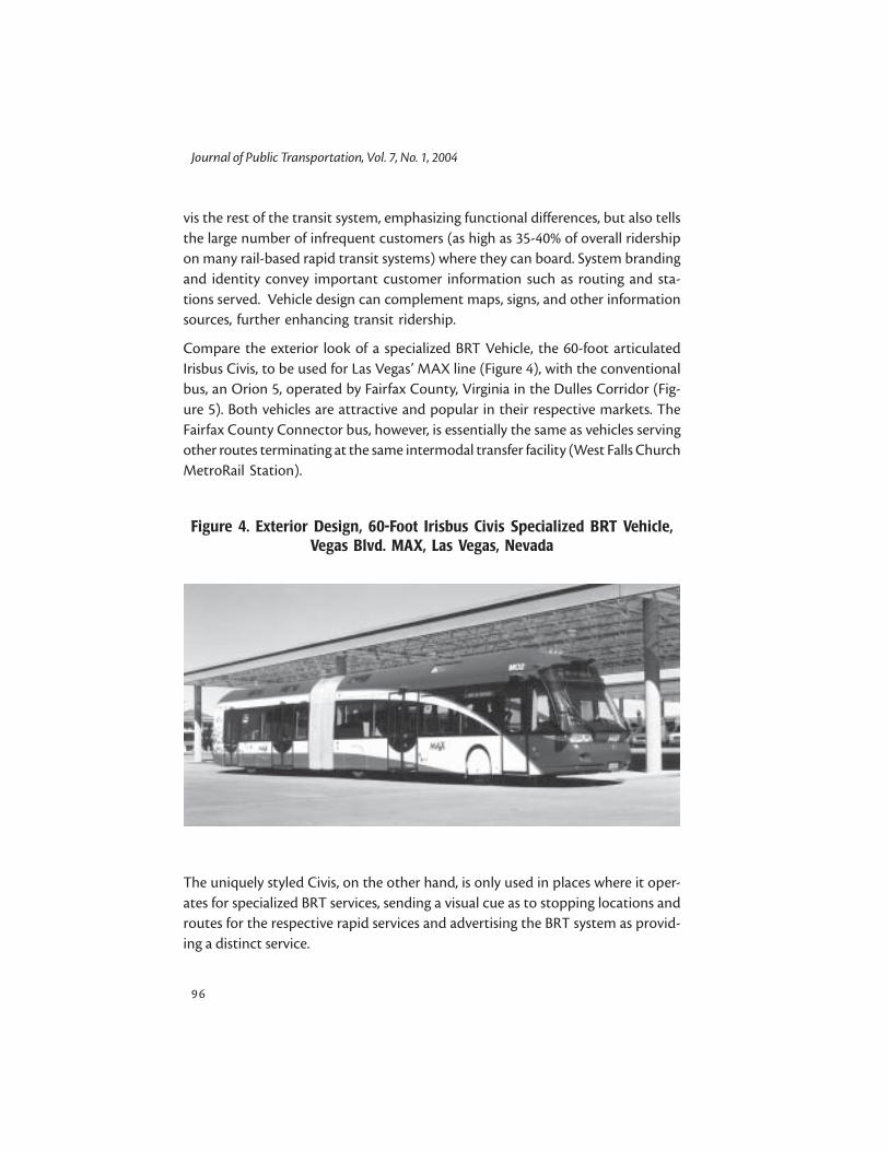
Journal of Public Transportation, Vol. 7, No. 1, 2004
9 6
vis the rest of the transit system, emphasizing functional differences, but also tellsthe large number of infrequent customers (as high as 35-40% of overall ridershipon many rail-based rapid transit systems) where they can board. System brandingand identity convey important customer information such as routing and sta-tions served. Vehicle design can complement maps, signs, and other informationsources, further enhancing transit ridership.
Compare the exterior look of a specialized BRT Vehicle, the 60-foot articulatedIrisbus Civis, to be used for Las Vegas’ MAX line (Figure 4), with the conventionalbus, an Orion 5, operated by Fairfax County, Virginia in the Dulles Corridor (Fig-ure 5). Both vehicles are attractive and popular in their respective markets. TheFairfax County Connector bus, however, is essentially the same as vehicles servingother routes terminating at the same intermodal transfer facility (West Falls ChurchMetroRail Station).
Figure 4. Exterior Design, 60-Foot Irisbus Civis Specialized BRT Vehicle,Vegas Blvd. MAX, Las Vegas, Nevada
The uniquely styled Civis, on the other hand, is only used in places where it oper-ates for specialized BRT services, sending a visual cue as to stopping locations androutes for the respective rapid services and advertising the BRT system as provid-ing a distinct service.

Vehicle Selection for BRT: Issues and Options
9 7
The low floor CNG Neoplan articulated vehicle used on MBTA’s Silver Line inBoston (Figure 6) illustrates the creative use of color and livery on conventionalequipment to provide a distinct image and identity, matching the color, routename, and map color. Contrast that with the livery of the 40-foot Nova Bus RTSused in regular MBTA local bus service (Figure 7). Such a branded appearance candistinguish a bus in BRT operation from one in local bus service. The vehicle liveryand icon or flag should be different from other buses, but match that of BRTstops, stations, and terminals, information signs, graphics, and all printed matter.In this way, it emphasizes that BRT is an integrated system.
Figure 5. Exterior Livery and Design, Orion 5 40-Foot Bus, Fairfax CountyConnector Dulles Corridor Express Services, Fairfax, County, Virginia

Journal of Public Transportation, Vol. 7, No. 1, 2004
9 8
As of 2003, at least five European bus manufacturers (Irisbus, Bombardier, Neoplan,APTS/VDL, and Translohr) have designed and built specialized BRT vehicles withan LRV-like exterior appearance, interior, and other features such as guidance. InEurope and South America, Volvo has BRT vehicle projects under way, while inNorth America, both New Flyer (Invero) and North American Bus Industries
Figure 6. Exterior Livery, Neoplan 60-Foot CNG Articulated Bus,Silver Line, MBTA, Boston, Massachusetts
Figure 7. Exterior Livery, Nova Bus RTS 40-Foot Bus, Local Bus Service,MBTA, Boston, Massachusetts
Vehicle Selection for BRT: Issues and Options
9 9
(Compobus) have BRT vehicle projects either in production or close to the pro-duction of prototypes. Examples of their features include large sizes and distinctshapes (lengths from 45-83 feet [13.8 to 25 meters]), large, panoramic passengerwindows, dramatically curved front windscreens, multiple doors, lateral guid-ance/precision docking, quiet, internal combustion-electric hybrid propulsion,and the option for the driver position to be in the center of the vehicle.
ConclusionThe importance of vehicles to the overall success of BRT systems cannot be over-stated. Vehicle design affects every aspect of system performance and cost, andtheir appearance, both external and internal, is a key contributor to the system’simage, identity and position in the transportation marketplace.
Based on documented experience to date, the following general guidelines shouldbe considered in BRT system planning and project development:
• Vehicles should be planned and ultimately specified as a function of thetype of services offered (e.g., local versus express, mixed) and the nature ofthe markets served (e.g., short non-work non-home related trips versuslong home to work trips).
• Vehicles should provide sufficient passenger capacity at comfortable load-ing standards (i.e., 3 standees per square meter in North America) foranticipated ridership levels and planned service structure and frequencies.Lengths ranging from 40-45 feet (12.2 - 13.75 meters) for single unit ve-hicles through double articulated (82-foot [25 meters]) vehicles are insuccessful revenue service and can be considered.
• Vehicles should have high passenger appeal, be environmentally friendly,easy and convenient to use, and comfortable. Desirable features includeair conditioning, bright lighting, panoramic windows, and real-time pas-senger information.
• Vehicles should be easy and rapid to board and alight. Low floor heights(i.e., less than 15 inches [38 cm]) above pavement level) are desirable unlesstechnologies permitting safe and reliable level boarding and alighting (e.g.,rapidly deployed ramps/bridges, some type of precision docking mecha-nism) can be used.
• A sufficient number of doors having sufficient width should be provided,especially where off-board fare collection is provided. Generally, one door

Journal of Public Transportation, Vol. 7, No. 1, 2004
100
channel should be provided for each ten feet of vehicle length. Vehicleswith doors on either or both sides are available and can enable use of sideand/or center platform stations.
• The mix of space devoted to standees and seating will depend on the typeof service and nature of the market served (e.g., express versus local). Be-cause a seated passenger occupies more space than a standee, total capac-ity is higher where the number of seats is lower, all else being equal.
• Wide aisles and sufficient circulation space can lower dwell times and allowfor better distribution of passengers, especially to the rear of articulatedvehicles.
• Cost-effective bus propulsion systems are available for revenue service that,compared to conventional diesel engine/hydraulic mechanical systems:
- virtually eliminate particulate emissions
- are environmentally friendly in terms of CO, HC and NOx emissions
- are relatively quiet
- get improved fuel economy
- accelerate faster.
• There are mechanical and electronic guidance systems in revenue servicethat can enable rail-like passenger boarding and alighting convenienceand service times at stations, reduce right-of-way requirements, and pro-vide a more comfortable ride than conventional buses.
• Vehicles should be well proven in revenue service before being introducedin large numbers for intense BRT operations. Controlling risk is extremelyimportant in the operation of highly visible services.
• BRT operations with standard vehicles in use on other parts of the respec-tive system are acceptable, as long as distinct livery (color schemes), graph-ics, icons, and other means are employed to provide a unique identity andimage. No special features are required to provide acceptable capacity,levels of service, and passenger attractiveness.
• Even where standard buses are used for BRT operations, considerationshould be given to internal layouts and door numbers and configurationsconsistent with the markets served and service provided.

Vehicle Selection for BRT: Issues and Options
101
• Use of specialized BRT vehicles is often desirable for high volume trunkroutes where the operational benefits of the specialized vehicles will offsettheir incremental costs.
• Cost should be considered on a life cycle basis, as some of the features thatadd to initial acquisition costs (e.g., guidance, hybrid drives, stainless steelframes, and composite bodies) have the potential to reduce ongoing op-erating and maintenance costs, increase passenger revenue, and add tovehicle service life.
• It is critical that vehicle planning and design be fully integrated with plan-ning and design for other BRT elements such as running ways, stations,fare collection, and service plans, if the overall system is to achieve its maxi-mum effectiveness and efficiency.

Journal of Public Transportation, Vol. 7, No. 1, 2004
102
References
Levinson, H., S. L. Zimmerman, J. Clinger, S. Rutherford, R. L. Smith, J. Cracknell,and R. Soberman. 2003. TCRP Report 90: Bus Rapid Transit, Volume 1: Case Studiesin Rapid Transit. Washington, DC: Transportation Research Board of the NationalAcademies.
Levinson, H., S. L. Zimmerman, J. Clinger, S. Rutherford, R. L. Smith, J. Cracknell,and R. Soberman. 2003a. TCRP Report 90: Bus Rapid Transit, Volume 2: Implemen-tation Guidelines. Washington, DC: Transportation Research Board of the Na-tional Academies.
Danaher, A. and P. Ryus. 1999. TCRP Project A-15. Transit Capacity and Quality ofService Manual, 1st Ed. Washington, DC: Transportation Research Board.
Bradley and Associates. 2000. Hybrid Electric Drive Heavy Duty Testing Project FinalEmissions Report. Boston, MA: Northeast Advanced Vehicle Coalition, West Vir-ginia University.
Vehicle Selection for BRT: Issues and Options
103
About the Authors
SAM ZIMMERMAN ([email protected]) is principal of the transpor-tation planning section of DMJM+HARRIS. His 34-year career has focused onrapid transit planning, transit economics and finance, and travel demand fore-casting. Mr. Zimmerman has consulted extensively on rapid transit and transpor-tation planning projects, planning procedures, and policy throughout the U.S.and the world, and has written numerous papers. He was co-principal Investiga-tor for the Transportation Research Board’s Bus Rapid Transit (BRT) Implementa-tion Guidelines project, and is project manager for the National Transit Institute’sBRT Training course.
HERBERT LEVINSON ([email protected]) is one of the world’s leading experts intraffic engineering, parking, transit planning, and the nexus between transit andtraffic operations. He has authored over 150 papers, edited and otherwise con-tributed to numerous transportation planning and traffic engineering books,taught at major universities such as Yale and New York Polytechnic Institute, per-formed research for the USDOT, the American Association of Automobile Manu-facturers, and the Transportation Research Board (TRB), and has consultedthroughout the world. Mr. Levinson is a member of the National Academy ofEngineering and serves on the Executive Committee of the Transportation Re-search Board. He was co-principal investigator for the Transportation ResearchBoard’s Bus Rapid Transit Implementation Guidelines project.