garcia-valle, rodrigo joel (2007) dynamic modelling...
TRANSCRIPT

Glasgow Theses Service http://theses.gla.ac.uk/
Garcia-Valle, Rodrigo Joel (2007) Dynamic modelling and simulation of electric power systems using the Newton-Raphson method. PhD thesis. http://theses.gla.ac.uk/435/ Copyright and moral rights for this thesis are retained by the author A copy can be downloaded for personal non-commercial research or study, without prior permission or charge This thesis cannot be reproduced or quoted extensively from without first obtaining permission in writing from the Author The content must not be changed in any way or sold commercially in any format or medium without the formal permission of the Author When referring to this work, full bibliographic details including the author, title, awarding institution and date of the thesis must be given

UNIVERSITY OF GLASGOW
Department of Electronics and Electrical Engineering
Dynamic Modelling and Simulation
of Electric Power Systems Using
the Newton-Raphson Method
by
Rodrigo Joel Garcia-Valle
A Thesis submitted to theDepartment of Electronics and Electrical Engineering
of theUniversity of Glasgow
for the degree ofDoctor of Philosophy
c© Rodrigo Joel Garcia-ValleDecember, 2007

To my parents and sister,for their hearten,
trust and love
To my beloved wife, Lorenaas a symbol of my love
and her forbearanceduring this years
To my lovely daughter, Valeriaas a gift on her birthday.
Abstract
The research work presented in this thesis is concerned with the development of a dynamicpower flow computer algorithm using Newton’s method. It addresses both the developmentof a positive sequence dynamic power flow algorithm for the dynamic study of balanced powersystems and a fully-fledged three-phase dynamic power flow algorithm for the dynamic studyof power systems exhibiting a significant degree of either structural or operational unbalance.
As a prelude to the research work on dynamic power flows, a three-phase Newton-Raphsonpower flow algorithm in rectangular co-ordinates with conventional HVDC power plant mod-elling is presented in this thesis, emphasising the representation of converter control modes.The solution approach takes advantage of the strong numerical convergence afforded by theNewton-Raphson method to yield reliable numerical solutions for combined HVAC-HVDCsystems, where power plant and operational imbalances are explicitly taken into account.
The dynamic algorithm is particularly suited to carrying out long-term dynamic simula-tions and voltage stability assessments. Dynamic model representations of the power plantscomponents and the load tap changing transformer are considered, and to widen the studyrange of dynamic voltage phenomena using this method, extensions have been made to includeinduction motor and polynomial load modelling features. Besides, reactive power compen-sators that base their modus operandi on the switching of power electronic valves, such as theHVDC-VSC and the STATCOM are taken into account. The dynamic power flow algorithmhas primarily been developed making use of the positive sequence and dq representations.Extensions are made to developing a three-phase power flows dynamic algorithm.
Test cases for the various dynamic elements developed in this research are presented toshow the versatility of the models and simulation tool, including a trip cascading event leadingup to a wide-area voltage collapse. Comparisons with the output of a conventional transientstability program carried out where appropriate.

Acknowledgments
The arduous effort that brings out doing a PhD thesis, will not be possible without theunestimated collaboration of many people. To all of you I want to dedicate this space toexpress my gratitude.
Firstly, I want to acknowledge to my supervisor, Prof. Enrique Acha, for the encourageand commitment given to me during all this period. He has always been up and keen to assistme at any time, giving me the necessary guidance and advice, but also being critic judgingmy work. I would like to express my thankfulness for his sincere friendship.
The National Council of Science and Technology, CONACyT Mexico, is gratefully ac-knowledge for the financial support provided during the research project.
I sincerely appreciate the collaboration work carried out by Federico Coffele, Luigi Van-fretti and Rafael Zarate during their work visit at the University of Glasgow; my truthfulgreet to Pedro Roncero for his fruitful comments about my thesis and his worthwhile adviceusing LATEX. I much appreciate their sincere friendliness.
I would like to express my thankfulness to my friends and colleges, Mykhaylo Teplechuk,Sven Soell, Maria Thompson, Damian Vilchis, Enrique Ortega and Carlos Ugalde for thetime, talks and outdoors experiences spent together; to the working environment at thepower system group at the department of electronics and electrical engineering and to itsentire staff.
And last but not least, I also fully appreciate the encourage and credence to me from myparents and sister during this long period. I truly acknowledge to my wife Lorena, for herlove, comprehension and encourage during latter years of hard work and sacrifices. And tomy daughter Valeria, for helping me to forget about my problem being with you. Withoutyou I would not had done it. THANKS.
Contents
1 Introduction 1
1.1 Overview . . . . . . . . . . . . . . . . . . . . . . . . . . . . . . . . . . . . . . 11.2 Objectives of the Project . . . . . . . . . . . . . . . . . . . . . . . . . . . . . 41.3 Contributions . . . . . . . . . . . . . . . . . . . . . . . . . . . . . . . . . . . . 61.4 Outline of the thesis . . . . . . . . . . . . . . . . . . . . . . . . . . . . . . . . 71.5 Publications . . . . . . . . . . . . . . . . . . . . . . . . . . . . . . . . . . . . . 9
2 Dynamic Assessment 10
2.1 Introduction . . . . . . . . . . . . . . . . . . . . . . . . . . . . . . . . . . . . . 102.2 Background Review . . . . . . . . . . . . . . . . . . . . . . . . . . . . . . . . 112.3 Literature Review . . . . . . . . . . . . . . . . . . . . . . . . . . . . . . . . . 142.4 Stability Evaluation . . . . . . . . . . . . . . . . . . . . . . . . . . . . . . . . 15
2.4.1 Steady-state stability . . . . . . . . . . . . . . . . . . . . . . . . . . . . 162.4.2 Transient stability . . . . . . . . . . . . . . . . . . . . . . . . . . . . . 172.4.3 Dynamic stability . . . . . . . . . . . . . . . . . . . . . . . . . . . . . 21
2.5 Off-line Functional Requirements . . . . . . . . . . . . . . . . . . . . . . . . . 222.5.1 Modelling and data conditions . . . . . . . . . . . . . . . . . . . . . . 222.5.2 Contingency analyses . . . . . . . . . . . . . . . . . . . . . . . . . . . 25
2.6 Dynamic Modelling Philosophy . . . . . . . . . . . . . . . . . . . . . . . . . . 262.7 The Trapezoidal Method . . . . . . . . . . . . . . . . . . . . . . . . . . . . . . 332.8 Summary . . . . . . . . . . . . . . . . . . . . . . . . . . . . . . . . . . . . . . 35
3 Newton-Raphson Power Flow Algorithm in abc Rectangular Co-ordinates 36
3.1 Introduction . . . . . . . . . . . . . . . . . . . . . . . . . . . . . . . . . . . . . 363.2 Power Flows Concepts . . . . . . . . . . . . . . . . . . . . . . . . . . . . . . . 37
3.2.1 The power flow problem formulation . . . . . . . . . . . . . . . . . . . 383.2.2 Power flow equations . . . . . . . . . . . . . . . . . . . . . . . . . . . . 39

Contents ii
3.2.3 The Jacobian matrix formation . . . . . . . . . . . . . . . . . . . . . . 403.2.4 Voltage controlled bus . . . . . . . . . . . . . . . . . . . . . . . . . . . 44
3.3 Power System Loads . . . . . . . . . . . . . . . . . . . . . . . . . . . . . . . . 453.4 Numerical Evaluation of a Multiphase Power Network . . . . . . . . . . . . . 483.5 HVDC Transmission Systems . . . . . . . . . . . . . . . . . . . . . . . . . . . 50
3.5.1 Converter steady state modelling . . . . . . . . . . . . . . . . . . . . . 523.5.2 Three-Phase Power Equations . . . . . . . . . . . . . . . . . . . . . . . 543.5.3 Linearised power equations . . . . . . . . . . . . . . . . . . . . . . . . 553.5.4 Control mode A . . . . . . . . . . . . . . . . . . . . . . . . . . . . . . 583.5.5 Control mode B . . . . . . . . . . . . . . . . . . . . . . . . . . . . . . 593.5.6 Control mode C . . . . . . . . . . . . . . . . . . . . . . . . . . . . . . 60
3.6 HVDC-LCC Numerical Evaluation . . . . . . . . . . . . . . . . . . . . . . . . 613.6.1 Test Case 1 . . . . . . . . . . . . . . . . . . . . . . . . . . . . . . . . . 613.6.2 Test Case 2 . . . . . . . . . . . . . . . . . . . . . . . . . . . . . . . . . 62
3.7 Summary . . . . . . . . . . . . . . . . . . . . . . . . . . . . . . . . . . . . . . 67
4 Dynamic Power Flows in Rectangular Co-ordinates 68
4.1 Introduction . . . . . . . . . . . . . . . . . . . . . . . . . . . . . . . . . . . . . 684.2 Synchronous Machine Model - Classical Representation . . . . . . . . . . . . 704.3 Synchronous Machines Controllers . . . . . . . . . . . . . . . . . . . . . . . . 74
4.3.1 Governor . . . . . . . . . . . . . . . . . . . . . . . . . . . . . . . . . . 744.3.2 Turbine . . . . . . . . . . . . . . . . . . . . . . . . . . . . . . . . . . . 754.3.3 Automatic voltage regulator . . . . . . . . . . . . . . . . . . . . . . . . 774.3.4 Boiler . . . . . . . . . . . . . . . . . . . . . . . . . . . . . . . . . . . . 79
4.4 Synchronous Machine Model - Advanced Representation . . . . . . . . . . . . 794.5 Network Modelling . . . . . . . . . . . . . . . . . . . . . . . . . . . . . . . . . 814.6 Transmission Line Model . . . . . . . . . . . . . . . . . . . . . . . . . . . . . 824.7 Dynamic Load Tap Changer and Phase Shifting Transformer Modelling . . . 834.8 Numerical Solution Technique . . . . . . . . . . . . . . . . . . . . . . . . . . . 854.9 Time Domain Simulations . . . . . . . . . . . . . . . . . . . . . . . . . . . . . 93
4.9.1 Validation . . . . . . . . . . . . . . . . . . . . . . . . . . . . . . . . . . 934.9.2 A classical stability study . . . . . . . . . . . . . . . . . . . . . . . . . 954.9.3 Test case 1 . . . . . . . . . . . . . . . . . . . . . . . . . . . . . . . . . 984.9.4 Test case 2 . . . . . . . . . . . . . . . . . . . . . . . . . . . . . . . . . 1014.9.5 Test case 3 . . . . . . . . . . . . . . . . . . . . . . . . . . . . . . . . . 102
4.10 Summary . . . . . . . . . . . . . . . . . . . . . . . . . . . . . . . . . . . . . . 107
Contents iii
5 Power System Loads Modelling 108
5.1 Load Modelling Concepts . . . . . . . . . . . . . . . . . . . . . . . . . . . . . 1085.1.1 Introduction . . . . . . . . . . . . . . . . . . . . . . . . . . . . . . . . 108
5.2 Static Load Model . . . . . . . . . . . . . . . . . . . . . . . . . . . . . . . . . 1115.2.1 Polynomial representation . . . . . . . . . . . . . . . . . . . . . . . . . 1115.2.2 Exponential representation . . . . . . . . . . . . . . . . . . . . . . . . 112
5.3 Frequency Load Model . . . . . . . . . . . . . . . . . . . . . . . . . . . . . . . 1135.4 Dynamic Load Model . . . . . . . . . . . . . . . . . . . . . . . . . . . . . . . 114
5.4.1 Induction motor modelling . . . . . . . . . . . . . . . . . . . . . . . . 1145.5 Results . . . . . . . . . . . . . . . . . . . . . . . . . . . . . . . . . . . . . . . . 121
5.5.1 Test case 1 . . . . . . . . . . . . . . . . . . . . . . . . . . . . . . . . . 1215.5.2 Test case 2 . . . . . . . . . . . . . . . . . . . . . . . . . . . . . . . . . 1245.5.3 Test case 3 . . . . . . . . . . . . . . . . . . . . . . . . . . . . . . . . . 1295.5.4 Test case 4 . . . . . . . . . . . . . . . . . . . . . . . . . . . . . . . . . 130
5.6 Summary . . . . . . . . . . . . . . . . . . . . . . . . . . . . . . . . . . . . . . 138
6 Modelling of FACTS Controllers 139
6.1 Introduction . . . . . . . . . . . . . . . . . . . . . . . . . . . . . . . . . . . . . 1396.2 Static Synchronous Compensator (STATCOM) . . . . . . . . . . . . . . . . . 1406.3 STATCOM Modelling . . . . . . . . . . . . . . . . . . . . . . . . . . . . . . . 1436.4 Numerical Evaluation of Power Networks with STATCOM Controller . . . . . 146
6.4.1 Test case 1 . . . . . . . . . . . . . . . . . . . . . . . . . . . . . . . . . 1466.4.2 Test case 2 . . . . . . . . . . . . . . . . . . . . . . . . . . . . . . . . . 1486.4.3 Test case 3 . . . . . . . . . . . . . . . . . . . . . . . . . . . . . . . . . 151
6.5 High Voltage Direct Current (HVDC) . . . . . . . . . . . . . . . . . . . . . . 1546.5.1 Voltage Source Converters - HVDC . . . . . . . . . . . . . . . . . . . . 155
6.6 VSC-HVDC Modelling . . . . . . . . . . . . . . . . . . . . . . . . . . . . . . . 1576.7 Numerical Evaluation of Power Networks with VSC-HVDC Controller . . . . 160
6.7.1 Test case 4 . . . . . . . . . . . . . . . . . . . . . . . . . . . . . . . . . 1606.8 Summary . . . . . . . . . . . . . . . . . . . . . . . . . . . . . . . . . . . . . . 164
7 Three-Phase Dynamic Power Flows in abc Co-ordinates 165
7.1 Introduction . . . . . . . . . . . . . . . . . . . . . . . . . . . . . . . . . . . . . 1657.2 Power System Modelling . . . . . . . . . . . . . . . . . . . . . . . . . . . . . . 166
7.2.1 Three-phase synchronous machine modelling . . . . . . . . . . . . . . 1667.2.2 Dynamic three-phase load tap changer model . . . . . . . . . . . . . . 169
Contents iv
7.2.3 Three-phase power loads . . . . . . . . . . . . . . . . . . . . . . . . . . 1737.3 Dynamic Simulations of Three-Phase Power Networks . . . . . . . . . . . . . 178
7.3.1 Test case 1 . . . . . . . . . . . . . . . . . . . . . . . . . . . . . . . . . 1787.3.2 Test case 2 . . . . . . . . . . . . . . . . . . . . . . . . . . . . . . . . . 1817.3.3 Test case 3 . . . . . . . . . . . . . . . . . . . . . . . . . . . . . . . . . 1867.3.4 Test case 4 . . . . . . . . . . . . . . . . . . . . . . . . . . . . . . . . . 190
7.4 Summary . . . . . . . . . . . . . . . . . . . . . . . . . . . . . . . . . . . . . . 194
8 Conclusions 195
8.1 Future work . . . . . . . . . . . . . . . . . . . . . . . . . . . . . . . . . . . . . 196
Bibliography 197
A HVDC Power Equations 206
B Jacobian Matrix Elements 210
B.1 Jacobian Elements - Partial Derivatives . . . . . . . . . . . . . . . . . . . . . 210B.2 Discretised State Variables . . . . . . . . . . . . . . . . . . . . . . . . . . . . . 211
C Power Networks Test Data 215
List of Figures
1.1 Basic elements of a power system. . . . . . . . . . . . . . . . . . . . . . . . . 2
2.1 Stable and unstable system. . . . . . . . . . . . . . . . . . . . . . . . . . . . . 182.2 Power angle characteristics. . . . . . . . . . . . . . . . . . . . . . . . . . . . . 202.3 Time frame of various transient phenomena. . . . . . . . . . . . . . . . . . . . 232.4 Software environment to carry out static and dynamic power flows calculations. 302.5 Flow diagram for dynamic power flows studies. . . . . . . . . . . . . . . . . . 312.6 Newton-Raphson flow diagram for dynamic power flows calculations. . . . . . 32
3.1 Three-phase transmission line diagram. . . . . . . . . . . . . . . . . . . . . . . 393.2 Flow diagram for three-phase power flows using the Newton-Raphson method
in rectangular co-ordinates. . . . . . . . . . . . . . . . . . . . . . . . . . . . . 463.3 One-line schematic representation of the 3 generators 9 buses power system. . 483.4 Bus voltage magnitude for unbalanced loading conditions. . . . . . . . . . . . 493.5 Monopolar HVDC system. . . . . . . . . . . . . . . . . . . . . . . . . . . . . . 523.6 HVDC-LCC monopolar converter station. . . . . . . . . . . . . . . . . . . . . 523.7 Asymmetric three-phase voltages. . . . . . . . . . . . . . . . . . . . . . . . . . 533.8 Unbalanced converter voltage waveform. . . . . . . . . . . . . . . . . . . . . . 543.9 Five-bus test network for three-phase balanced conditions. . . . . . . . . . . . 613.10 Modified 16 generators power network. . . . . . . . . . . . . . . . . . . . . . . 633.11 Tap position of link 2, Control Mode A. . . . . . . . . . . . . . . . . . . . . . 653.12 Firing and extinction angles of links 3 and 1, Control Mode B and C, respectively. 653.13 Direct current of links 1 and 3, Control Mode B and C, respectively. . . . . . 66
4.1 Synchronous machine scheme. . . . . . . . . . . . . . . . . . . . . . . . . . . . 734.2 IEEE simplified speed governor model. . . . . . . . . . . . . . . . . . . . . . . 754.3 IEEE steam turbine model. . . . . . . . . . . . . . . . . . . . . . . . . . . . . 764.4 STA1 IEEE AVR model. . . . . . . . . . . . . . . . . . . . . . . . . . . . . . . 78

List of Figures vi
4.5 Phasor diagram of synchronous generator in the transient state. . . . . . . . . 804.6 Phasor diagram of synchronous generator in the sub-transient state. . . . . . 824.7 Transmission line representation. . . . . . . . . . . . . . . . . . . . . . . . . . 834.8 Tap-changer transformer equivalent circuit. . . . . . . . . . . . . . . . . . . . 844.9 Dynamic load tap changer model. . . . . . . . . . . . . . . . . . . . . . . . . . 844.10 Discrete tap. . . . . . . . . . . . . . . . . . . . . . . . . . . . . . . . . . . . . 854.11 Bus voltage response to a load change. . . . . . . . . . . . . . . . . . . . . . . 944.12 PSAT simulation - Bus voltage response to a load change. . . . . . . . . . . . 944.13 Electrical power deliver by generators. . . . . . . . . . . . . . . . . . . . . . . 954.14 δi − δ1 response to the load change. . . . . . . . . . . . . . . . . . . . . . . . . 964.15 Synchronous generators’ angular velocity. . . . . . . . . . . . . . . . . . . . . 964.16 3 Generators 9 buses power system. . . . . . . . . . . . . . . . . . . . . . . . 974.17 Bus voltage response to the fault. . . . . . . . . . . . . . . . . . . . . . . . . . 984.18 δi responses to the fault. . . . . . . . . . . . . . . . . . . . . . . . . . . . . . . 984.19 δij differences. . . . . . . . . . . . . . . . . . . . . . . . . . . . . . . . . . . . . 994.20 Speed deviation ωi response to the fault. . . . . . . . . . . . . . . . . . . . . . 994.21 Voltage magnitude for generator buses. . . . . . . . . . . . . . . . . . . . . . . 1004.22 Synchronous generators’ mechanical power. . . . . . . . . . . . . . . . . . . . 1004.23 Synchronous generators’ excitation voltage. . . . . . . . . . . . . . . . . . . . 1014.24 Bus voltage magnitude. . . . . . . . . . . . . . . . . . . . . . . . . . . . . . . 1014.25 Dynamic Load Tap-Changer (DLTC) performance. . . . . . . . . . . . . . . . 1024.26 Voltage magnitude at Buses 4, 7 and 9. . . . . . . . . . . . . . . . . . . . . . 1034.27 One-line New England test system diagram. . . . . . . . . . . . . . . . . . . . 1044.28 Bus voltages’ response. . . . . . . . . . . . . . . . . . . . . . . . . . . . . . . . 1054.29 Dynamic load tap changer performance. . . . . . . . . . . . . . . . . . . . . . 1054.30 Voltage magnitude at Bus 3. . . . . . . . . . . . . . . . . . . . . . . . . . . . 106
5.1 Simple load representation as ZIP loads. . . . . . . . . . . . . . . . . . . . . . 1125.2 Induction motor equivalent circuit. . . . . . . . . . . . . . . . . . . . . . . . . 1145.3 Single-cage induction motor representation. . . . . . . . . . . . . . . . . . . . 1225.4 Static load model representation. . . . . . . . . . . . . . . . . . . . . . . . . . 1225.5 Bus voltage magnitude at Bus 2. . . . . . . . . . . . . . . . . . . . . . . . . . 1235.6 Active power injection at Bus 2. . . . . . . . . . . . . . . . . . . . . . . . . . 1245.7 Reactive power injection at Bus 2. . . . . . . . . . . . . . . . . . . . . . . . . 1245.8 Air-gap voltage profile. . . . . . . . . . . . . . . . . . . . . . . . . . . . . . . . 1255.9 Slip performance. . . . . . . . . . . . . . . . . . . . . . . . . . . . . . . . . . . 125
List of Figures vii
5.10 Bus frequency deviation. . . . . . . . . . . . . . . . . . . . . . . . . . . . . . . 1265.11 Active power consumption by the induction motors. . . . . . . . . . . . . . . 1265.12 Reactive power consumption by the induction motors. . . . . . . . . . . . . . 1275.13 Slip performance. . . . . . . . . . . . . . . . . . . . . . . . . . . . . . . . . . . 1275.14 Bus voltage magnitude at load-connected buses. . . . . . . . . . . . . . . . . . 1285.15 Generators’ field voltage. . . . . . . . . . . . . . . . . . . . . . . . . . . . . . . 1285.16 Active power consumption of the induction motor. . . . . . . . . . . . . . . . 1295.17 Reactive power consumption of the induction motor. . . . . . . . . . . . . . . 1305.18 Slip performance of the induction motor. . . . . . . . . . . . . . . . . . . . . . 1305.19 Bus voltage profile. . . . . . . . . . . . . . . . . . . . . . . . . . . . . . . . . . 1315.20 Generators’ speed. . . . . . . . . . . . . . . . . . . . . . . . . . . . . . . . . . 1315.21 One-line New England test system diagram. . . . . . . . . . . . . . . . . . . . 1325.22 Bus voltage profile - Loads as induction motors. . . . . . . . . . . . . . . . . . 1335.23 Bus voltage profile - Loads with exponential indices equal to 1. . . . . . . . . 1345.24 Active power consumed by the induction motors. . . . . . . . . . . . . . . . . 1355.25 Reactive power consumed by the induction motors.. . . . . . . . . . . . . . . 1355.26 Voltage magnitudes at N14. . . . . . . . . . . . . . . . . . . . . . . . . . . . . 1365.27 Slip performance. . . . . . . . . . . . . . . . . . . . . . . . . . . . . . . . . . . 1365.28 Slip performance. . . . . . . . . . . . . . . . . . . . . . . . . . . . . . . . . . . 137
6.1 STATCOM one-line diagram. . . . . . . . . . . . . . . . . . . . . . . . . . . . 1416.2 STATCOM model. . . . . . . . . . . . . . . . . . . . . . . . . . . . . . . . . . 1436.3 STATCOM block diagram. . . . . . . . . . . . . . . . . . . . . . . . . . . . . 1446.4 Bus voltage response to a load change. . . . . . . . . . . . . . . . . . . . . . . 1476.5 STATCOM voltage injection. . . . . . . . . . . . . . . . . . . . . . . . . . . . 1476.6 STATCOM reactive power injection. . . . . . . . . . . . . . . . . . . . . . . . 1486.7 Bus voltage profile for condition when NO STATCOM is placed. . . . . . . . 1496.8 Bus voltage profile for condition when STATCOM is placed. . . . . . . . . . . 1496.9 Reactive power injection of the STATCOM. . . . . . . . . . . . . . . . . . . . 1506.10 Voltage magnitude injection of the STATCOM. . . . . . . . . . . . . . . . . . 1506.11 STATCOM current absorbtion. . . . . . . . . . . . . . . . . . . . . . . . . . . 1516.12 Bus voltage magnitude when STATCOM device is connected. . . . . . . . . . 1526.13 Voltage magnitude comparison at Bus 14. . . . . . . . . . . . . . . . . . . . . 1526.14 Bus voltage magnitude when no STATCOM device is connected. . . . . . . . 1536.15 Reactive power injected by the STATCOM. . . . . . . . . . . . . . . . . . . . 1536.16 STATCOM voltage. . . . . . . . . . . . . . . . . . . . . . . . . . . . . . . . . 154
List of Figures viii
6.17 HVDC-VSC transmission link diagram. . . . . . . . . . . . . . . . . . . . . . 1586.18 HVDC control block diagram for the rectifier stage. . . . . . . . . . . . . . . 1586.19 HVDC control block diagram for the inverter stage. . . . . . . . . . . . . . . 1596.20 HVDC based VSC equivalent circuit. . . . . . . . . . . . . . . . . . . . . . . . 1596.21 Bus voltage response of the power network. . . . . . . . . . . . . . . . . . . . 1616.22 Bus voltage magnitude at HVDC terminals. . . . . . . . . . . . . . . . . . . . 1626.23 Bus voltage magnitude at Bus 7. . . . . . . . . . . . . . . . . . . . . . . . . . 1626.24 HVDC-VSC transferred power when dc link losses are considered. . . . . . . . 163
7.1 Schematic synchronous machine representation. . . . . . . . . . . . . . . . . . 1687.2 Dynamic load tap changer model. . . . . . . . . . . . . . . . . . . . . . . . . . 1707.3 Schematic representation of the discrete tap changer. . . . . . . . . . . . . . . 1717.4 Star-star transformer connection. . . . . . . . . . . . . . . . . . . . . . . . . . 1717.5 Star-delta transformer connection. . . . . . . . . . . . . . . . . . . . . . . . . 1727.6 Delta-delta transformer connection. . . . . . . . . . . . . . . . . . . . . . . . . 1727.7 Star-connected load representation. . . . . . . . . . . . . . . . . . . . . . . . . 1747.8 Delta-connected load representation. . . . . . . . . . . . . . . . . . . . . . . . 1747.9 Three-phase bus voltage magnitude under unbalanced loading conditions. . . 1797.10 Three-phase bus voltage magnitude under balanced loading conditions. . . . . 1807.11 Three-phase voltage magnitude at Bus 5 under balanced and unbalanced load-
ing conditions. . . . . . . . . . . . . . . . . . . . . . . . . . . . . . . . . . . . 1817.12 Synchronous generators speed deviation under unbalanced loading conditions. 1817.13 Synchronous generators speed deviation under balanced loading conditions. . 1827.14 Rotor angle deviation under unbalanced loading conditions. . . . . . . . . . . 1827.15 Rotor angle deviation under balanced loading conditions. . . . . . . . . . . . 1837.16 Rotor angle differences under unbalanced loading conditions. . . . . . . . . . 1837.17 Bus voltage magnitude under unbalanced condition. . . . . . . . . . . . . . . 1847.18 Angle differences under unbalanced condition. . . . . . . . . . . . . . . . . . . 1857.19 Angle differences under balanced condition. . . . . . . . . . . . . . . . . . . . 1857.20 Rotor speed deviation under unbalanced condition. . . . . . . . . . . . . . . . 1867.21 Rotor speed deviation under balanced condition. . . . . . . . . . . . . . . . . 1867.22 Bus voltage magnitude for phase a under balanced condition. . . . . . . . . . 1877.23 Phase a of the bus voltage magnitude for voltage-controlled buses. . . . . . . 1877.24 Phase b of the bus voltage magnitude for voltage-controlled buses. . . . . . . 1887.25 Phase c of the bus voltage magnitude for voltage-controlled buses. . . . . . . 1887.26 Dynamic load tap changer performance. . . . . . . . . . . . . . . . . . . . . . 189
List of Figures ix
7.27 Field voltage magnitude for synchronous generators . . . . . . . . . . . . . . . 1897.28 Three-phase active power consumption by the induction motor connected at
Bus 5. . . . . . . . . . . . . . . . . . . . . . . . . . . . . . . . . . . . . . . . . 1907.29 Three-phase active power consumption by the induction motor connected at
Bus 6. . . . . . . . . . . . . . . . . . . . . . . . . . . . . . . . . . . . . . . . . 1917.30 Three-phase reactive power consumption by the induction motor connected at
Bus 5. . . . . . . . . . . . . . . . . . . . . . . . . . . . . . . . . . . . . . . . . 1917.31 Three-phase reactive power consumption by the induction motor connected at
Bus 6. . . . . . . . . . . . . . . . . . . . . . . . . . . . . . . . . . . . . . . . . 1927.32 Slip performance for three-phase induction motor. . . . . . . . . . . . . . . . 1927.33 Voltage magnitude for induction motor-connected buses. . . . . . . . . . . . . 193
A.1 Six pulse converter station. . . . . . . . . . . . . . . . . . . . . . . . . . . . . 206A.2 Unbalanced converter voltage waveform. . . . . . . . . . . . . . . . . . . . . . 207
List of Tables
3.1 Unbalanced complex power loads. . . . . . . . . . . . . . . . . . . . . . . . . . 493.2 Data for the HVDC link. . . . . . . . . . . . . . . . . . . . . . . . . . . . . . . 623.3 Bus voltages and generation results. . . . . . . . . . . . . . . . . . . . . . . . 623.4 Powers from generator buses and HVDC converters. . . . . . . . . . . . . . . 623.5 HVDC link control modes. . . . . . . . . . . . . . . . . . . . . . . . . . . . . . 633.6 Parameters of Link 1. . . . . . . . . . . . . . . . . . . . . . . . . . . . . . . . 643.7 Parameters of Link 2. . . . . . . . . . . . . . . . . . . . . . . . . . . . . . . . 643.8 Parameters of Link 3. . . . . . . . . . . . . . . . . . . . . . . . . . . . . . . . 64
5.1 Induction Motor Parameters . . . . . . . . . . . . . . . . . . . . . . . . . . . . 123
6.1 STATCOM parameters . . . . . . . . . . . . . . . . . . . . . . . . . . . . . . . 146
7.1 Final values for power loads. . . . . . . . . . . . . . . . . . . . . . . . . . . . . 179
C.1 Transmission line parameters: Five-bus test system . . . . . . . . . . . . . . . 215C.2 Generation: Five-bus test system . . . . . . . . . . . . . . . . . . . . . . . . . 215C.3 Power loads: Five-bus test system . . . . . . . . . . . . . . . . . . . . . . . . 216C.4 Power transformers: New England system . . . . . . . . . . . . . . . . . . . . 216C.5 Transmission line parameters: New England system . . . . . . . . . . . . . . 217C.6 Generation: New England system . . . . . . . . . . . . . . . . . . . . . . . . . 218C.7 Power loads: New England system . . . . . . . . . . . . . . . . . . . . . . . . 218C.8 Transmission line parameters: Three-generators, nine-bus system . . . . . . . 219C.9 Generation: Three-generators, nine-bus system . . . . . . . . . . . . . . . . . 219C.10 Power loads: Three-generators, nine-bus system . . . . . . . . . . . . . . . . . 219C.11 Power transformers: Three-generators, nine-bus system . . . . . . . . . . . . 219

List of Symbols and Acronyms
Capital letters
P Active power
Pag Active power at the air-gap
Pl Active load power
PdR Active power at the rectifier
Ka Amplifier gain
Ta Amplifier time constant
Ae First ceiling coefficient
Be Second ceiling coefficient
Se Ceiling function
I Complex current
S Complex power
V Complex voltage
Iq Quadrature axis current
Idq Axis armature current
Id Direct axis current
xi

List of Symbols and Acronyms xii
Idc Current at the dc link
Ia Phase a current
D Damping coefficient
∆− Y Delta-star connection
Te Field circuit time constant
BC1 Fire intensity
BC2 Auxiliary variable
K Governor gain
Pgov Governor power
T1 Governor time constant
Zl Series impedance
Yl Shunt impedance
H Inertia constant
J Jacobian matrix
Tr Measurement time constant
Mg Angular momentum
abc abc frame of reference
Pe Electrical power
Pa Power of the synchronous generator
Pm Mechanical power
PM Equivalent mechanical input powers
Pkm Active power through the phase shifter
Pset Power set point
List of Symbols and Acronyms xiii
Q Reactive power
Qag Reactive power at the air-gap
QdI Reactive power at the inverter
Ql Reactive load power
Xr Rotors’ reactance
Rr Rotors’ resistance
Ysc Short-circuit admittance matrix
Kf Stabiliser gain
Tf Stabiliser time constant
Y −∆ Star-delta connection
Y − Y Star-star connection
SF Steam production
Tk Tap ratio
A Tap changer position
HT Taps’ servomotor inertia
P0 Target active power
V0 Target voltage magnitude
DP Throttle pressure
T ′do Transient time constant at the d axis
T ′′do Sub-transient time constant at the d axis
T ′qo Transient time constant at the q axis
T ′′qo Sub-transient time constant at the q axis
FHP High pressure turbine power fraction

List of Symbols and Acronyms xiv
PHP High pressure turbine power
FIP Intermediate pressure turbine power fraction
PIP Intermediate pressure turbine power
FLP Low pressure turbine power fraction
PLP Low pressure turbine power
TCH Steam chest time constant
TCO Cross-over or steam storage time constant
TRH Reheat time constant
Vd Voltage magnitude at the d axis
Ea Excitation or behind the reactance voltage
E′d Flux linkage voltage at the d axis
E′q Flux linkage voltage at the q axis
VdI Voltage at the inverter
Vq Voltage magnitude at the q axis
VdR Voltage at the rectifier
Vr Regulator voltage
Lowercase letters
ra Armature resistance
k3 Boiler gain
dq0 dq0 frame of reference
e Real part of the voltage
f Imaginary part of the voltage
List of Symbols and Acronyms xv
fag Imaginary voltage at the air-gap
it Iterations
nbus Number of buses
ngen Number of synchronous generators
j Mathematical complex operator√−1
k1 Constant associated with commutation overlap
x′d Transient quadrature reactance at the d axis
xd Direct axis reactance
x′′d Sub-transient quadrature reactance at the d axis
x′q Transient quadrature reactance at the q axis
xq Quadrature axis reactance
x′′q Sub-transient quadrature reactance at the q axis
eag Real voltage at the air-gap
s Rotor’ slip
y State variable
f0 Synchronous frequency
x Vector of integrable algebraic variables
y Vector of non-integrable algebraic variables
Greek symbols
σ Acceleration
α Firing angle
∆ Increment
List of Symbols and Acronyms xvi
ε Round-off error
γ Extinction angle
µ Exponential load model constant
ν Exponential load model constant
ρ Denote phases a, b, c
θ Phase angle
φk Phase angle mechanism on the primary side
δ Power or rotor angle
δ0 Initial power angle
ω Synchronous generator speed
ω0 Synchronous speed
Acronyms
ABB Asea Brown Boveri
AC Alternate Current
AVR Automatic Voltage Generator
CCC Capacitor Commutated Converter
CIGRE Conseil International des GrandsReseaux Electriques
CPF Continuation Power Flows
FPC Federal Power Commission
NYPP New York Power Pool
CPU Central Processing Unit
DAE Differential-Algebraic Equations

List of Symbols and Acronyms xvii
DC Direct Current
DLTC Dynamic Load Tap Changer
FACTS Flexible Alternate Current Transmission Systems
GTO Gate Turn-Off thyristor
SVC Static VAR Compensator
HVDC High Voltage Direct Current
IEEE The Institute of Electrical and Electronics Engineers
IGBT Insulated Gate Polar Transistor
LCC Line Commutated Current
LTC Load Tap Changer
NERC North American Electric Reliability Council
ODE Ordinary Differential Equation
OEL Over Excitation Limiter
PES Power Engineering Society
PSAT Power System Analysis Toolbox
QSS Quasi-Static Simulation
USA United States of America
VSC Voltage Source Converter
Chapter 1
Introduction
1.1 Overview
Electric power systems around the world are all of different sizes; each having its own
generation, mix transmission structure and load capacity to serve. Nevertheless, all of them
share similar construction and operating principles, with four main elements becoming, at
first sight, more visible, namely generating units, transmission lines, transformers and loads.
Control and protection equipment have a vital function to play and they also constitute essen-
tial elements of the electric power system. Arguably, from a dynamic viewpoint, generating
units and loads are the most important elements of the electric power system.
Electric power is generated mainly using synchronous machines, which are driven by
turbines of various kinds, such as steam, hydro, diesel, nuclear and internal combustion. The
generator voltages are in the range of 11 to 35 kV [Kundur, 1994]. The generating stations
may be far away from consumers centres and transmission lines make up the link between
distribution systems, where the loads are, and generating units. The transmission system
is said to be the backbone of any electric power system and operates at high voltage levels
(commonly, 230 kV-400 kV). Distribution voltage levels are typically in the range 4 kV - 34.5
kV. Industrial consumers are fed from primary feeders at these voltage levels; residential and
1.1. Overview 2
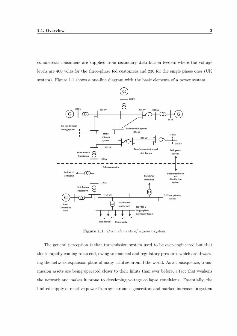
commercial consumers are supplied from secondary distribution feeders where the voltage
levels are 400 volts for the three-phase fed customers and 230 for the single phase ones (UK
system). Figure 1.1 shows a one-line diagram with the basic elements of a power system.
Tie line to neigh-
boring system
20 kV 500 kV
22 kV
24 kV
Tie line
500 kV 230 kV
Trans-
mission
system
500 kV
Transmission system
230 kV
230 kV
To subtransmission and
distribution
345 kV
Residential Commercial
120/240 V
Single-phase
Secondary feeder
115 kV
Subtransmission
Bulk power
system
Subtransmission
and
distribution
system
Transmission
Substation
Industrial
consumer
Distribution
substation
Small
Generating
Unit
3 -Phase primary
feeder
115 kV
12.47 kV
Industrial
consumer
Distribution
transformer
G
G G
G
Figure 1.1: Basic elements of a power system.
The general perception is that transmission system used to be over-engineered but that
this is rapidly coming to an end, owing to financial and regulatory pressures which are thwart-
ing the network expansion plans of many utilities around the world. As a consequence, trans-
mission assets are being operated closer to their limits than ever before, a fact that weakens
the network and makes it prone to developing voltage collapse conditions. Essentially, the
limited supply of reactive power from synchronous generators and marked increases in system
1.1. Overview 3
load are factors that contribute to increase the likelihood of voltage instabilities. If at a given
point in time and space, these adverse matters come together and the situation is not man-
aged appropriately, a local voltage instability may reach neighbouring equipment becoming
more widespread and leading to a voltage collapse. In extreme cases, the voltage collapse
may engulf the entire power system or a large geographical area encompassing neighbouring
systems; an instance know by the public at large as a ”blackout”. Owing to the high social
and economic costs that instances of voltage collapse carry, the power engineering community
has made the study of this phenomenon a high profile issue.
Based on recent experience, gained from carrying out very detailed post-mortum analyses
of a series of major operational disasters which took place in the Autumn of 2003, the
North American Electric Reliability Council (NERC) developed system and planning operator
standards for controlling and avoiding such undesirable situations. The key recommendations
of the NERC document are summarised as follows:
1. Generation and demand must balance continuously.
2. Reactive power supply and demand must balance to maintain scheduled voltages.
3. Monitor power flows transmission lines and other equipment to ensure that thermal
(heating) limits are not exceeded.
4. Keep the system in a stable condition.
5. Operate the system in such a way that it remains in a reliable condition even if a
contingency were to occur, such as the loss of a key generation or transmission facility.
6. Plan, design, and maintain the system in such a way that it operates reliably.
7. Prepare for emergencies.
Despite the techniques and methodologies available to keep blackouts and outages at
1.2. Objectives of the Project 4
bay, most practising engineers concur that the most practical way to prevent blackouts from
happening is to carry out comprehensive long-term voltage stability simulations.
Excessive imbalances in the phase voltages or currents of a three-phase power system have
always been a concern to power engineers. Moreover, a typical power system may contain
untransposed transmission lines and feeders, single and unbalanced three-phase static loads,
single and three-phase dynamic loads such as induction motors, co-generators, transformers,
capacitors banks and more advanced power electronics systems, such as FACTS devices. To
try to incorporate a suitable representation of the impact that excessive imbalances have in
the power system, a three-phase dynamic power flow algorithm which considers the complete
power system is developed in this research work.
The solution algorithm combines the differential equations that represent the network
dynamic with the algebraic equations that represent the static part, in such a way that
a simultaneous method becomes possible. The technique possesses the advantage of being
numerically stable. It is robust and capable of handling islanding and simultaneous faults. It
must be said that the conventional methods of power systems simulation (transient stability-
like algorithms) are known to incur problems when network islanding arises [Kundur, 1994,
Machowski et al., 1997]. Such key advantage of the dynamic simulator developed in this
research will be exploited to study blackouts and long-term dynamic assessments.
1.2 Objectives of the Project
The main objective of this PhD project is to conduct research on the dynamic modelling,
simulation and assessment long-term power system dynamics using the Newton-Raphson
method in rectangular co-ordinates.
A key aspect of paramount importance in this research is the development of new math-
ematical models and methods coded into software to carry out effective dynamic analyses of
power networks. The software is robust and flexible enough to solve power networks undergo-
1.2. Objectives of the Project 5
ing different circumstances, including steady-state operating conditions, electromechanical-
type transients and slow voltage oscillations.
On the main, this PhD thesis is developed within the broad context of voltage stability,
focusing on aspects of dynamic modelling of power plat components. These models are
suitably combined with those of conventional sources of reactive power such as synchronous
generators and those pertaining to a new bread of reactive power compensators that base
their modus operandi on the switching of power electronic valves, such as HVDC-VSC and
FACTS controllers. It describes fundamental concepts regarding power systems stability
analysis, time domain dynamics simulations of non-linear power systems in the combined
use of the positive sequence and dq representations. The software developed is aimed at the
study of long-term power systems dynamic when unfavourable conditions of the system are
present. The FACTS devices, including HVDC-VSC control, the load modelling and the
synchronous machines have been all selected and modelled to be amenable with the objective
of this research work.
It has been observed in practice that voltage collapse phenomena may evolve over time
scales that are several times the orders of magnitude of power systems phenomena studied
with well-established transient stability application methods, such as those looking at first
and second swing assessments. Hence, in order to ensure numerically stable solutions, even
when rather large integration time steps are used, which may become necessary in the kind
of studies that fall within the remit of this research; a simultaneous approach that uses
the implicit trapezoidal rule in conjunction with the Newton-Raphson method is applied
to carry out the time domain simulations. Again this contrast with the solution methods
used in conventional transient stability application programs where the time-dependent nodal
currents at the generator nodes are injected into a nodal impedance matrix.
The software developed in this research provides a flexible and robust test bed where the
impact of traditional and emerging power system controllers on long-term dynamic simula-
tions can be tested with ease.
1.3. Contributions 6
1.3 Contributions
The main contributions of the research work are summarised below:
• A complete methodology for a developing dynamic power flow algorithm using Newton’s
method in rectangular co-ordinates has been developed. A flexible digital computer
program has been written in MATLAB. This is a flexible simulation tool for the study
of dynamic reactive power assessments and voltage stability phenomena.
• A general framework of reference for the solution of unified dynamic power flow solutions
problems is presented.
• A dq model of the synchronous generator with saliency and flux decay has been imple-
mented within the dynamic power flow algorithm, to enable suitable representation of
the fast dynamic effects contributed by the synchronous generators.
• To widen the study range of dynamic voltage phenomena using the dynamic power flow
algorithm, induction motor modelling features have been developed. For completeness,
voltage and frequency dependant load models have also implemented.
• A discrete dynamic LTC transformer model suitable for the dynamic power flow algo-
rithm has also been developed, implemented and applied to assess its impact on the
voltage collapse phenomena.
• A Static Synchronous Compensator model which takes account of the dynamics of the
device is developed and suitably included into the dynamic power flow algorithm.
• The implementation of a High Voltage Direct Current link model based on voltage-
source converter is presented. In general, VSC-FACTS controllers are devices of great
flexibility and speed of response, which aid the power system response during both
normal and abnormal operation, as shown in this research.

1.4. Outline of the thesis 7
• A fully-fledged three-phase dynamic power flow algorithm using abc co-ordinates is
developed to study power networks with significant degree of unbalance.
• A comprehensive and robust three-phase power flow algorithm in rectangular co-ordinates
is developed.
• Conventional LCC-HVDC controllers with different control operating modes have been
introduced.
1.4 Outline of the thesis
This PhD thesis is organised in 8 chapters, including this introductory chapter, taking
the following structure.
Chapter 2 outlines the main concepts involved in power system stability, describing the
main kinds of stability and their importance in power systems planning and operation. A
global definition of the power system stability is given. In addition, the modelling and data
required to carry out voltage stability assessments are discussed. The all-important problem
of contingency analyses is brought into discussion. The justification for selecting a dynamic
modelling approach to study power system contingencies and related problems of voltage
stability is given. The integration method applied in this research to solve the differential
equations that characterise the electrical power systems is described.
Chapter 3 presents the theory of phase domain power flows using rectangular co-ordinates.
Starting from first principles, it derives the nodal power flows equations, the Jacobian matrix
entries and the linearised three-phase power flow equations. In order to expand the flexibility
representation of contemporary power systems, LCC-HVDC are modelled on a three-phase
basis. To make this representation more realistic, three different control strategies for LCC-
HVDC links are developed. Test cases of unbalanced multi-phase power networks are solved,
using different control modes.
1.4. Outline of the thesis 8
Chapter 4 focuses on the dynamic power flow algorithm using the Newton-Raphson
method in rectangular co-ordinates. The traditional power system elements and the con-
ventional synchronous machine representation with its classical controllers such as governor,
turbine, automatic voltage regulator and boiler are considered and suitably modelled within
the dynamic power flow algorithm. An advanced synchronous machine model which con-
siders the transient saliency and flux linkages in each axis of the synchronous machine is
implemented. A realistic tap changer transformer model for dynamic assessments taking due
account of the discrete nature of the transformer tap, is developed. The basic dynamic power
flow algorithm is discussed in a comprehensive manner in this chapter. A classical transient
stability study, validation results for the solution technique and some test cases are included.
Chapter 5 deals with power system load modelling. It stresses the importance of load
modelling in dynamic studies, and critically assesses the most popular static and dynamic
load models used in stability analyses. An induction motor load model and its inclusion into
the dynamic power flow algorithm, is put forward. Several case studies are presented using
different load representations. An assessment of the response of the static load models and
that of an induction motor model is presented.
Chapter 6 is dedicated to the modelling and simulation of FACTS devices based on
voltage source converters. The STATCOM and HVDC-VSC are single out for development
and their inclusion into the dynamic power flow algorithm. Several tests cases are solved,
where the control improvements in the power system response when the STATCOM and
HVDC controllers are used, is clearly shown.
Chapter 7 deals with the extension of the basic dynamic power flow algorithm into a full
three-phase dynamic power flow algorithm in ABC co-ordinates. The algorithm is suitably
applied to the dynamic assessments of unbalanced power systems. The dynamic load tap
changer and the static and dynamic load models are expressed in ABC co-ordinates and
implemented in the three-phase dynamic power flow algorithm.
Chapter 8 draws overall conclusions for this research work and suggests directions for

1.5. Publications 9
future research work in this timely area of electric power systems.
1.5 Publications
During the process of this doctoral thesis and as part of it, the following publications
have been generated.
• F. Coffele, R. Garcia-Valle and E. Acha, ”The Inclusion of HVDC Control Modes in a
Three-Phase Newton-Raphson Power Flow Algorithm”. Paper presented at the IEEE
Power Tech Conference, Lausanne, Switzerland, July 2007.
• R. Garcia-Valle and E. Acha, ”The Incorporation of a Discrete, Dynamic LTC Trans-
former Model in a Dynamic Power Flow Algorithm”. Paper presented at the Power
and Energy Systems EuroPES Conference IASTED, Palma de Mallorca, Spain, August
2007.
Chapter 2
Dynamic Assessment
2.1 Introduction
The maintenance of stability between the rotating masses of all the synchronous generators
in the power network and system load is an essential requirement for the operation any
electrical power system. Within its limits, all the equipment in the network naturally tends
to operate in synchronism, and it is very important to understand where the limits lays and
how close to such limits the system can be pushed and still maintain normal operation.
Stability studies, such as small signal, transient rotor angle and voltage stability studies
are effective tools for the evaluation of power system performance under abnormal operating
conditions. Besides, the usefulness of these studies is in the design and implementation of
control strategies for the enhancement of the overall stability of the system.
To be able to carry out these studies, it becomes first necessary to use the adequate
mathematical models of synchronous machines, prime movers, voltage regulators and the
broad number of control systems involved in the dynamic operation of power systems. Thus,
the results derived from any stability simulation directly relies on the mathematical models
of each one of the devices taken into consideration.
This chapter deals with general aspects of power system stability. A background and lit-
2.2. Background Review 11
erature on the subject are presented to lay the ground for the description and classification of
power system stability phenomena, together with the modelling and data set required to carry
out voltage stability assessments are presented. The justification for the dynamic modelling,
simulation and analyses is presented towards the end of the chapter. The Chapter concludes
with a brief description of the trapezoidal method of integration. The integration method
applied to solve the differential equations that characterise the electrical power systems is
reported.
2.2 Background Review
Power systems around the world are being faced with great many challenges concerning
overall system security, reliability and stability issues because of the unprecedented increase
in electricity demand, limited transmission expansion, and the fact that new power plants
are not being built close to the population centers because of environmental, land availability
and economic constraints. Several major blackouts [US - Canada Power System Outage Task
Force, 2004,Knight, 2001], exemplify these issues rather well.
One of the most sever power failures in history was experienced in November 1965 in the
United Stated. This blackout lasted for about 19 hours, affecting millions of people.
The main technical reason behind the disturbance was the faulty setting of a relay and the
resulting tripping of one of five heavily loaded 230-kilovolts transmission lines [IEEE Power
Engineering Review, 1991].
After such a disaster the Federal Power Commission (FPC), which was the regulatory
body overseeing the American power system at the time, prepared a report for the president
of the USA, with a recommendations to create the Northeast Reliability Council (NERC)
and the New York Power Pool (NYPP). Both institutions have developed industry standards
for equipment testing and reserve generation capacity, as well as promoted the reliability of
bulk electric utility systems in North America.
2.2. Background Review 12
Notwithstanding all this effort, a new outage occurred in 1977 in New York city. The
new blackout was a consequence of a combination of natural phenomena, mal operation of
protective devices, inadequate presentation of data to system dispatchers and communication
difficulties [Corwin and Miles, 1998]. Such adverse combination of conditions led to a wide-
area voltage collapse in the Consolidated Edison system; the Consolidate Edison system is
one of the 8 members of the New york Power Pool (NYPP) and it supplies electricity to five
regions of New York city Manhattan, the Bronx, Brooklyn, Queen and Westchester Country.
Following on the steps of these two large blackouts, many others wide-area voltage col-
lapses have happened in the USA, fortunately the consequences were not as severe as the
previous two. Nevertheless, in the months of July and August of 1996, events turned for
the worst; the USA underwent another two large-scale blackouts. These system failures took
the industry by surprise since generation from the Pacific Northwest had been at its all time
peak.
For the case of the July’s blackout, the main reason was a flashover in a tree and near
a 345-kV line, the faulty operation of a ground unit of an analogue electronic relay, and a
voltage depression in the Southern Idaho system. All of this led to the new fatal blackout.
In August 1996, the generation capability and the power transfer from Canada to the
USA was at almost peak value but the weather was very warm. Over a period of time, the
power grid started to overload due to insufficient generation. This outage affected more that
4 million people in the USA and even in some parts of Mexico.
Within the last five years, a series of blackouts have struck many countries around the
world. A case in point is Italy, which is a country highly dependent on electricity supplies
from neighbouring countries. The blackout occurred due to branches of a tree falling on a
380-kV transmission line coming from neighbouring Switzerland, resulting the remaining lines
in corridor becoming overloaded. Furthermore, two transmission lines coming from France
came out of operation. Following these events, the whole of Italy suffered a power outage,
with the exception of the island of Sardinia [Commission de Regulation de L’energie, 2004].
2.2. Background Review 13
Another recent, is the blackout that took place in London, where the system failure was
traced to a wrongly installed fuse at a key power station. [National Grid, 2003].
The latest most recent blackout took place, once more in the USA. This outage has
been attributed to the loss of generation in Cleveland power station which was, in turn,
due to the sequential loss of three overloaded 345-kV transmission lines in Ohio, South of
Cleveland. The unbalance between load and generation produced a cascading effect leading
to the blackout [US - Canada Power System Outage Task Force, 2004].
Other key aspects which are making the system more fragile, is the way in which the inter-
connected system is being operated, transferring power in large blocks from generation excess
areas to generation deficit points, thus leading to increased transmission congestion problems.
Power system operators are constantly dealing with the challenge of operating their systems
in a secure manner, while taking into account the uncertainty in demand and supply and the
availability of enough security margins. Thus, off-line system studies are performed to ensure
the overall system security ahead of time. In addition to the static application studies dealing
with the constrained optimal operation of the network, dynamic studies are also carried out.
These are mainly classified into voltage stability analysis and angle stability analysis, based
on short-, mid- and long-term stability studies. These dynamic studies are based on power
system models that are represented by differential-algebraic equations (DAEs); by necessity,
these mathematical models are based on approximate system representation and limited data,
since obtaining comprehensive and reliable data for a power system is a rather troublesome
task [Concordia and Ihara, 1982].
In spite of the many investigations into methods of assessing voltage stability such as,
Liapunov’s method, continuation power flows, extended equal-area criterion, bifurcation anal-
yses, a different way to approach this issue is the use of simultaneously solution techniques.
This method is numerically more stable than the traditionally solution algorithms, robust
and inherent capable of handling islanding and fault analyses [Gear, 1971b, Rafian et al.,
1987].

2.3. Literature Review 14
This thesis studies various issues regarding off-line modelling of power system, i.e. long-
term stability analysis, which are associated with phenomena that may lead to significant
problems in power systems. The possibility of predicting the voltage collapse using these
system simultaneous solution technique combined with the Newton-Raphson method is ex-
plored, as the dynamic effect of the different system plant components, load modelling and
FACTS devices models on the unified frame-of-reference.
2.3 Literature Review
Over the years, various computational methods have been developed to carry out off-
line and on-line security assessments of the power system enabling prediction and corrective
actions of problematic dynamic system instances.
These tools have been developed to carry out more realistic dynamic reactive power system
margins and voltage collapse assessments. The existing computer programs use one of the
following approaches: Quasi-Static Simulation (QSS), Continuation Power Flows (CPF).
The QSS uses a suitable combination of detailed dynamic models and simplified steady state
models [Van Cutsem and Vournas, 1998]. The s-domain is used to access the problem of
voltage collapse from a dynamic perspective; carrying out sensitivity analyses to determine
the nature of the equilibrium point with data information obtained from a state estimator
[IEEE Power Engineering Society, 2002]. Continuation power flows takes the approach of
tracing the PV-curves to determine the critical equilibrium point [Qin et al., 2006].
In spite of the great numerical robustness, modelling capabilities and software flexibilities
of these application tools, they may not be able to take into account the full dynamics of
power system elements. Besides, these simulation approaches may not be able to incorporate
protection action, the long term dynamics response of the system after short-circuit events
and when islanding conditions. These factors are important issues to be considered when
carrying out voltage stability assessments.
2.4. Stability Evaluation 15
An alternative solution approach for the study of voltage phenomena based on full time
domain simulations is developed in this thesis. It is a unified framework where the power
flows representation of the network is combined with the dynamic models of the power system
to enable combined solutions at pre-defined discrete time steps using the Newton-Raphson
method. The result is a dynamic power flows algorithm where all dynamic components in
the power system are fully taken into account.
These off-line tools may be used by system operators to gain information on available
security margins and in taking proper corrective actions to overcome system problems.
2.4 Stability Evaluation
Power system stability is a term denoting a condition in which the various synchronous
machines of the system remain in synchronism with one another [Kimbark, 1948a]. The
IEEE/CIGRE joint Task Force on stability [IEEE/CIGRE Joint Task Force on Stability
Terms and Definitions, 2004] has defined the problem of power system stability as follows:
”Power system stability is the ability of an electric power system, for a given initial oper-
ating condition, to regain a state of operating equilibrium after being subjected to a physical
disturbance, with most system variables bounded so that practically the entire system remains
intact.”
Power system stability has always been recognized as an important issue for secure system
operation [IEEE/CIGRE Joint Task Force on Stability Terms and Definitions, 2004], and
the many blackouts caused by system instability highlight the importance of the problem
[IEEE Power Engineering Review, 1991, Anderson et al., 2005]. As power systems have
evolved through continuing growth in voltage and power rating and interconnections have
sprawled, different forms of stability have emerged. Hence, a classification of the problem of
power system stability has become necessary. This is a key issue which needs to be clearly
understood to be able to properly design, operate and control an electrical power system.
2.4. Stability Evaluation 16
The current steady-state stability consensus is that power system stability can be classified
into steady-state stability, transient stability and dynamic stability.
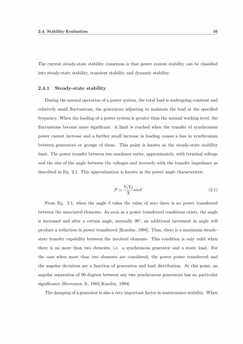
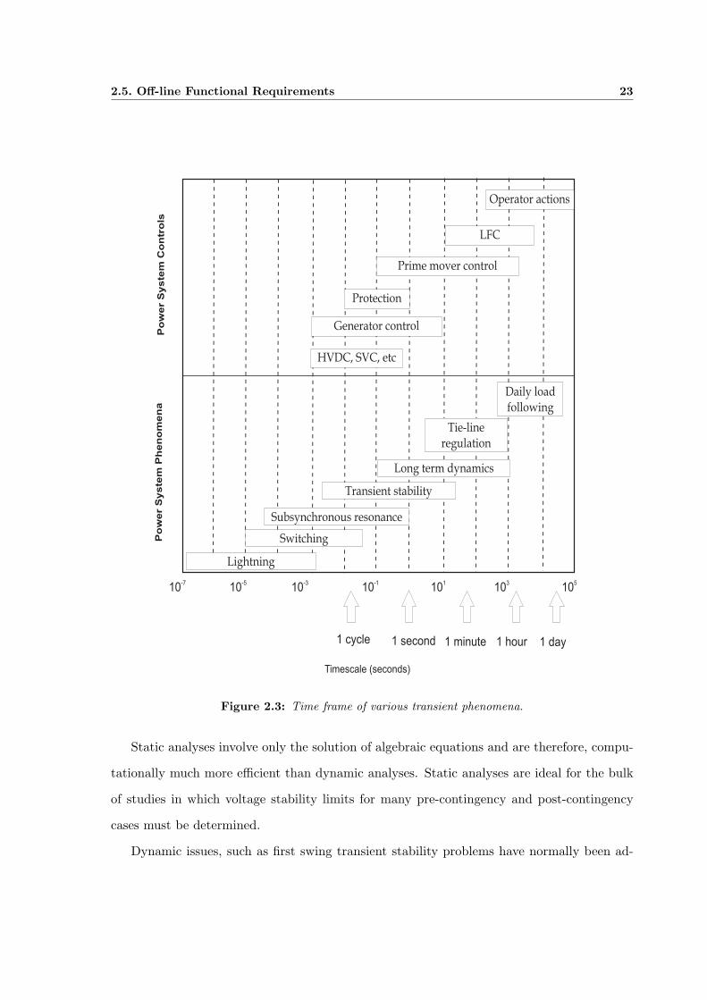
2.4.1 Steady-state stability
During the normal operation of a power system, the total load is undergoing constant and
relatively small fluctuations, the generators adjusting to maintain the load at the specified
frequency. When the loading of a power system is greater than the normal working level, the
fluctuations become more significant. A limit is reached when the transfer of synchronism
power cannot increase and a further small increase in loading causes a loss in synchronism
between generators or groups of them. This point is known as the steady-state stability
limit. The power transfer between two machines varies, approximately, with terminal voltage
and the size of the angle between the voltages and inversely with the transfer impedance as
described in Eq. 2.1. This approximation is known as the power angle characteristic.
P ' V1V2
Xsinδ (2.1)
From Eq. 2.1, when the angle δ takes the value of zero there is no power transferred
between the associated elements. As soon as a power transferred conditions exists, the angle
is increased and after a certain angle, normally 90◦, an additional increment in angle will
produce a reduction in power transferred [Kundur, 1994]. Thus, there is a maximum steady-
state transfer capability between the involved elements. This condition is only valid when
there is no more than two elements, i.e. a synchronous generator and a static load. For
the case when more than two elements are considered, the power power transferred and
the angular deviation are a function of generation and load distribution. At this point, an
angular separation of 90 degrees between any two synchronous generators has no particular
significance [Stevenson Jr, 1982,Kundur, 1994].
The damping of a generator is also a very important factor in maintenance stability. When

2.4. Stability Evaluation 17
the damping is positive, transients due to load fluctuations die out; when it has a value equal
to zero, the machines could remain stable and when negative, the oscillations increase and
the angle between voltages eventually exceed the limit.
The addition of an automatic voltage regulator improves the stability of a synchronous
generator. By making excitation a function of the power output, the terminal voltage is
varies, which in turn varied the steady-state stability limit.
2.4.2 Transient stability
When a change in load occurs, the synchronous generator cannot respond immediately,
due to the inertia of its rotating parts. To identify if the system is stable after a disturbance
it is necessary to solve the generator’s swing equation. The system is unstable if the angle
of a synchronous generator or between any two of them tends to increase without limit. On
the other hand, if the angle reaches a maximum value and then decrease, the system may be
stable. There is a simple and direct method for assessing the stability of the system, but it
may only apply to systems of no more than generators. It is know as the equal-area stability
criterion [Kimbark, 1948a, Stevenson Jr, 1982] and does not require an explicit solution of
the generator’s swing equation. Some simplifying assumptions are:
• The mechanical power is constant
• The synchronous generator is represented by a voltage source of constant magnitude
behind a transient reactance.
The swing equation describes the synchronous generator rotor dynamics through a differ-
ential equation of the form:

2.4. Stability Evaluation 18
Md2δ
dt2= Pa (2.2)
Pa = Pm − Pe (2.3)
where
δ is the rotor angle.
M is the inertia constant.
Pa is the accelerating power.
Pm is the mechanical power.
Pe is the electrical power.
The key concept behind the equal-area criterion is illustrated in Fig. 2.1 where an unstable
and a stable condition are presented. In the unstable case, δ increases indefinitely with time
and the machine loses synchronism. In contrast, the stable case undergoes oscillations, which
eventually disappear because of damping. It is clear that in the stable case the gradient od
the δ-curve reaches a value of 0, i.e. dδdt = 0.
Stable
Unstable
0=dt
dd
2d
1d
0d
d
t
Figure 2.1: Stable and unstable system.
Therefore the stability is checked by monitoring the rotor speed deviation dδdt , with respect
to the synchronous speed, which must be zero at some point, this means that:
2.4. Stability Evaluation 19
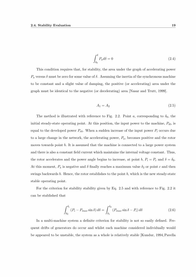
∫ δ
δ0
Padδ = 0 (2.4)
This condition requires that, for stability, the area under the graph of accelerating power
Pa versus δ must be zero for some value of δ. Assuming the inertia of the synchronous machine
to be constant and a slight value of damping, the positive (or accelerating) area under the
graph must be identical to the negative (or decelerating) area [Nasar and Trutt, 1999].
A1 = A2 (2.5)
The method is illustrated with reference to Fig. 2.2. Point a, corresponding to δ0, the
initial steady-state operating point. At this position, the input power to the machine, Pi0, is
equal to the developed power Pe0. When a sudden increase of the input power Pi occurs due
to a large change in the network, the accelerating power, Pa, becomes positive and the rotor
moves towards point b. It is assumed that the machine is connected to a large power system
and there is also a constant field current which maintains the internal voltage constant. Thus,
the rotor accelerates and the power angle begins to increase, at point b, Pi = Pe and δ = δ0.
At this moment, Pa is negative and δ finally reaches a maximum value δ2 or point c and then
swings backwards b. Hence, the rotor establishes to the point b, which is the new steady-state
stable operating point.
For the criterion for stability stability given by Eq. 2.5 and with reference to Fig. 2.2 it
can be stablished that
∫ δi
δ0
(Pi − Pmax sin δ) dδ =∫ δ2
δ1
(Pmax sin δ − Pi) dδ (2.6)
In a multi-machine system a definite criterion for stability is not so easily defined. Fre-
quent drifts of generators do occur and whilst each machine considered individually would
be appeared to be unstable, the system as a whole is relatively stable [Kundur, 1994,Pavella

2.4. Stability Evaluation 20
maxsin
eP P d=
iP
P
maxP
0iP
2A
1A
b
c
a
0d
1d
2d
P
d
Figure 2.2: Power angle characteristics.
and Murthy, 1995,Machowski et al., 1997].
Transient stability studies are usually performed for a frame time of a few seconds follow-
ing the disturbance. In the case of two machine systems, if the system first-swing is stable,
then stability is usually assured. For multi-machine systems, it is necessary to prolong the
study to ensure that interactions between synchronous generator swinging do not induce in-
stabilities in other generators during the second or third swing. By the end of the the third
swing, the amplitude of the oscillations are usually diminishing and if the system is still stable
there is little chance of later instability.
The problem of stability during the transient period is usually most acute when faults
occur in the electrical network. The most common fault is that of a single-phase being
short-circuited to ground, but the most onerous is normally a three-phase short-circuit.
When a fault occurs the transfer impedance rises instantaneously to a new value and the
power-angle curve changes. The generators accelerate because of power unbalance between
the mechanical and the electrical powers. Normally faults are cleared quickly by opening the
circuit breakers before the clearing critical time.
2.4. Stability Evaluation 21
2.4.3 Dynamic stability
When a system is working close to the stability limit even or when operating in a dynami-
cally stable region, small perturbations such as those normally experienced in a power-system,
may cause instability. This situation has become more pronounced recently as large blocks
of power are transmitted over very long distances. The model of the system for dynamic
stability studies must be very accurate and the software used for the study must include
components not normally modelled in software used for transient stability studies. In studies
of this type the simulation time is very long, lasting up to tens of minutes of time phenomena
representation.
If for any reason the transfer impedance between the synchronous generators and an
induction motor load increases, then a voltage reduction occurs which causes the motor to
slow down. This will cause an increment of current and reactive power flowing into the motors
and a further voltage decrement will follow. It is possible in a situation like this that the
voltage may collapse in the vicinity of the load. This is a voltage instability phenomena.
Stable operation of a power system depends on the ability to continuously match the
electrical output of generating units to the electrical load of the system. Dynamic stability
of power systems is a non-linear phenomenon which arises from the fact that generators are
operated in a parallel structure and during steady-state they are operated in synchronism.
The evaluation of a power systems’ ability to cope with large disturbances and to survive
transitions to normal or acceptable operating conditions it is termed transient stability assess-
ment. A transient period occurs when this equilibrium state is disturbed by a sudden change
in input, load, structure, or in a sequence of such changes; the system is transiently stable if
after a transient period, the system returns to a steady condition, maintaining synchronism.
If it does not, it is unstable and the system may be divided into disconnected subsystems,
which in turn may experience further instability.
During the dynamic stability, there is a very common scenery called outages of voltage

2.5. Off-line Functional Requirements 22
collapse. This outages can be divided into two major groups, planned and unplanned outages.
The first ones are mainly related to the maintenance of equipment or upgrade of the
power network, whereas the latter ones are described by unscheduled events such as wrong
relay co-ordination scheme, unfavourable weather conditions or poor reactive power supply.
2.5 Off-line Functional Requirements
2.5.1 Modelling and data conditions
Experimentation with power system components is expensive and time consuming, there-
fore, simulations are a fast and economic method to conduct studies in order to analyse the
system performance and this type of devices. Power system elements should be designed to
endure overvoltages and faults. Due to the great electrical and mechanical stress that these
devices support during transient conditions, the design of these components relies on the
dynamic characteristics of these elements. Modelling and simulation are issues of paramount
importance in the design and operation of any power system.
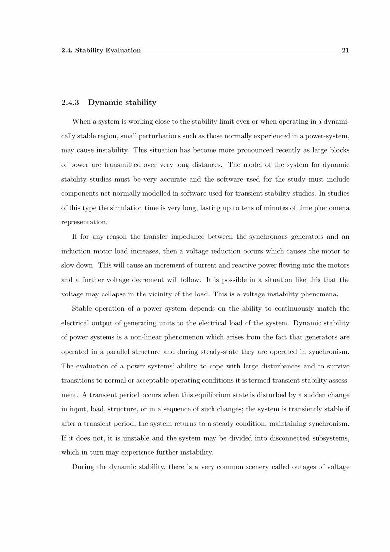
Correct modelling selection, should bare in mind the time-scale for the problem at hand.
Fig. 2.3 shows the main areas for the power systems’ dynamic assessment [Arrillaga and
Watson, 2002]. In principle at least, it is possible to develop a simulation model which consider
all the dynamic phenomena, from the fast inductive/capacitive effects of the network, to the
slow effects associated with plant dispatch, but this would be a very hard task and it is not
done in practice.
Traditionally, power system engineers have used two main classes of programs for analyses
of bulk power systems performance: 1) power flows and 2) transient stability.
Historically, power and reactive power flow problems have been analysed using static
power flow programs. This approach was satisfactory since these problems have been governed
by essentially static or time-independent factors. Power flow analyses allows simulation of a
snapshot of time.
2.5. Off-line Functional Requirements 23
Po
wer
Syste
m C
on
tro
lsP
ow
er
Syste
m P
hen
om
en
a
Operator actions
LFC
Prime mover control
Protection
Generator control
HVDC, SVC, etc
Daily loadfollowing
Tie-lineregulation
Long term dynamics
Transient stability
Subsynchronous resonance
Switching
Lightning
105
103
101
10-1
10-3
10-5
10-7
Timescale (seconds)
1 cycle 1 minute1 second 1 day1 hour
Figure 2.3: Time frame of various transient phenomena.
Static analyses involve only the solution of algebraic equations and are therefore, compu-
tationally much more efficient than dynamic analyses. Static analyses are ideal for the bulk
of studies in which voltage stability limits for many pre-contingency and post-contingency
cases must be determined.
Dynamic issues, such as first swing transient stability problems have normally been ad-

2.5. Off-line Functional Requirements 24
dressed using transient stability programs. These programs ordinarily include dynamic mod-
els of the synchronous machines with excitation systems, turbines and governors, as well as
other dynamic models, such as loads and fast acting devices. These component models and
the accompanying solution algorithms are suitable for analyses of phenomena from tens of
milliseconds up to several seconds.
With the evolution of modern, heavily compensated power systems, voltage stability has
emerged as the limiting consideration in many systems. The phenomenon of voltage collapse
is dynamic, yet frequently evolves very slowly, from the perspective of a transient stability
program. It has been argued that slower acting devices such as generator over excitation
limiters (OEL) and the characteristics of the system loads will contribute to the evolution
of a voltage collapse [IEEE Power Engineering Society, 2002,Sekine and Ohtsuki, 1990,Hill,
1993, Anrborg et al., 1998]. Power flow analysis will take into account all these effects, by
enforcement of their steady-state response, which is based on algebraic considerations. Con-
versely, transient stability analysis will typically assume that these phenomena are slow, and
corresponding variables will remain constant. In actual practice, neither of these assump-
tions can be relied upon, thus leaving voltage collapse in a no-mans-land between these two
analytical domains.
The recent emergence of a new class of computer simulation software provides utility
engineers with powerful tools for analysis of long-term dynamic phenomena. The ability to
perform long-term dynamic simulations with detailed dynamic modelling permits more accu-
rate assessment of critical power system problems than what it is possible with conventional
power flows and transient stability programs. However, time-domain simulations are time
consuming in terms of CPU and are essentially for post-mortem analyses and the coordina-
tion of protection and control. Therefore, the most effective approach for studying voltage
instability is to make use of an analytical technique which consider the full dynamics of an
electrical power network.
Conventional analytical tools, including power flows and transients stability programs may
2.5. Off-line Functional Requirements 25
not be particularly well suited to the analyses of all voltage stability problems. Specifically,
long term dynamic simulations require good models of the slow dynamics associated with
voltage collapse and also the modelling of important slow acting controls and protective
devices. This modelling technique will give utility engineers the ability to conduct studies
that reflect the behaviour of the systems in a more realistic manner. Moreover, the interaction
of customer loads and system equipment such as generator protection, load tap-changer
transformer control and shunt compensation plays a key role in the progress of a voltage
collapse.
The dynamic nature of the aggregate system load, that is, the change in characteristics
between the transient and the long-term period, has important consequences for analyses
of voltage stability. Modelling of frequency dependence of the loads may therefore be as
important as voltage dependence. So then, load behaviour is a main part of long-term
dynamic modelling.
There is a strong relationship between the load modelling and the modelling of other
system components, in terms of the overall system response. High fidelity simulations are
dependent on good representation of all these elements.
2.5.2 Contingency analyses
A contingency consists of one or more events happening simultaneously or at different
instants of time, with each event resulting in a change in the state of one or more power
system elements. A contingency may be initiated by a small disturbance, which may be a
fault, or a switching action.
It is impractical and unnecessary to analyse in detail the impact of every conceivable
contingency. Generally, only a limited number of contingencies might impose a immediate
threat to voltage stability and these might be different from the ones impacting on transient
stability. It is required therefore to define a reliable list of contingencies and provide the
capability to screen and select those most likely to cause problems, so that they will be

2.6. Dynamic Modelling Philosophy 26
addressed in detail.
The following types of switching operations should be considered as a contingency:
• Breaker opening/closing,
• Generator tripping,
• Load shedding.
For contingency analyses, the dynamic simulation should be able to analyse both fast
and slow dynamics, preferably with automatic time step adjustment. Besides, it should con-
tain generator and governor dynamics, tap changing time delays and prime mover dynamics
mainly.
2.6 Dynamic Modelling Philosophy
Before it is possible to study the methods of solving the electrical power-system stability
problem, it is necessary to adequately define the elements of the system in such a manner
that a time solution is both feasible and practical.
Engineering judgement must be used to establish the approximations, which can safely
be made in order that the model behaves in a similar manner to the actual system. Some of
the approximations have self-cancelling effects and can be justified, while others can be made
only where it leads to a pessimistic result.
The approximations are necessary harder to avoid the expense of an over-elaborate model
which would require an unduly large programme using excessive computer storage and exe-
cution time.
Another reason for the approximations is that data on the elements of the power-system
is limited and the models should reflect this limitation.
The classical model of a synchronous machine is that of a fixed voltage magnitude behind a
reactance. This model was adequate for investigations of multi-machine stability performance
2.6. Dynamic Modelling Philosophy 27
before the advent of digital computers. It led to pessimistic results often indicated that the
system was unstable when in practice it maintained stability. Models of machines close to
large disturbances were made more accurate accounting for changes in the flux linkages in
the field winding. This together with the inclusion of automatic voltage regulators (AVR)
actions, improved results by a considered margin. When digital computers became available
it was possible to further improve the results by including damper winding and speed governor
models. To compensate for the increased accuracy of the generator models, the representation
of loads was also improved, moving on from the constant impedance representation to include
constant power and constant current types. Moreover, large induction motors were beginning
to be modelled in a similar fashion to synchronous machines.
If only steady-state performance of the networks is on interest, it is standard to model the
networks by a set of non-linear equations, corresponding to the active and reactive powers
injected at the nodes of the network. The set of equations that describe the system for stability
studies may be more involved, and may be divided into two groups. Differential equations
are used to describe the rotational motion of synchronous generators and induction motors,
the slowly changing voltages representing the internal characteristics of the machines, and
their controllers.
The electrical network responds very rapidly to changes and a good assumption is that
the response is instantaneous. Algebraic equations therefore describe the network very well
for the range of phenomena which are of concern in this research. These equations are
linearised around a base operating point determined by the system load powers and the
mechanical/electrical power contributed by the generators in the system.
Variables associated with the differential equations must be solved using a suitable inte-
gration method and may be referred to as integrable variables. Similarly variables associated
with the algebraic equations may be referred to as algebraic or non-integrable variables.
Combing the two sets of equations, yields an algebraic-differential initial described as:
2.6. Dynamic Modelling Philosophy 28
y = F (y, x) (2.7)
0 = G (x, y) (2.8)
where x and y are vectors of integrable and non-integrable algebraic variables. The
starting conditions for the stability simulations are determined by using only the algebraic
set Eq. 2.8. This is followed by a combined solution of Eq. 2.7 and Eq. 2.8 as a function of
time, to be able to carry out the dynamic assessments.
In consequence, the objective of the dynamic assessment is to solve x and y as a function
of time.
Equation 2.7, comprises the differential equations of all synchronous generators and their
controllers. Since each generator is coupled to the power plants only through a single con-
necting bus of the network, Eq. 2.7 is a collection of separate subsets. Eq. 2.8 consists of
network equations and the stator equations of all synchronous generators transformed into
the network reference frame. The two set of equations are co-dependent so then the solution
technique should be a simultaneous one for high solution reliability. The open literature
offers a rich list of solution techniques [Kundur, 1994, Machowski et al., 1997, Pavella and
Murthy, 1995,Arrillaga, 1998,Van Cutsem and Vournas, 1998,Claudio A. Canizares, 1995].
In power system research there are two main approaches proposed to carry out the solution
of Eq. 2.7 and Eq. 2.8 [Stott, 1979]. In the first approach the solution of the algebraic and
differential equations is carried out in an independent fashion, and it is termed partitioned
method. The other solution approach consists in solving the algebraic and differential equa-
tions at the same time. The differential equations are transformed into algebraic equations
and combined with the network algebraic equations. This approach is termed simultaneous
approach method. The most common way of solving the sets of Eq. 2.7 and Eq. 2.8 to
carry out power system dynamic assessments, is to use the partitioned method. This remark
2.6. Dynamic Modelling Philosophy 29
applies to both academic and commercial software alike. there are two notable exceptions,
where the simultaneous method is applied very elegantly [Rafian et al., 1987, Van Cutsem
and Vournas, 1998].
For instance, Van Cutsem [Van Cutsem and Vournas, 1998], developed a technique for
voltage stability using a simultaneously method. This technique approaches the problem by
modelling only the slow dynamics, while the fast dynamics are neglected, converting them
into algebraic equations, enabling quasi-static simulation (QSS), as referred to by the author.
The solution technique adopted for voltage stability assessment in this work is a simulta-
neous method, which is based mainly in the simultaneous solution of the differential-algebraic
equations (DAEs) [Gear, 1971b,Rafian et al., 1987].
As a first approach, a dynamic power flow algorithm using the trapezoidal rule and the
Newton-Raphson technique has been developed. Moreover, this algorithm has been extended
to the phase co-ordinates system to cover situation of natural imbalances in the power network
and also cases of unbalanced loading. In either case, the balanced of the unbalanced solution
approach, the differential equations are discretised and transformed into algebraic equations
ensuing that the discretised equations are in such a way that can be solved in conjunction
with the algebraic equations.
The most important power plant components which should be modelled dynamically
for dynamic voltage assessments are: the synchronous generators and their controls (AVR,
turbine-governor, boiler), dynamic loads, load tap-changers and phase-shifters, and FACTS
controllers, bring out a reliable simultaneously technique for voltage stability assessment.
Figure 2.4 depicts the general algorithm developed during this research project. It con-
tains four main blocks. The first one makes provisions for all the relevant data related to
the power network, such as generation, loads, load-tap changers and FACTS equipment. The
second block encompasses a list of faults and perturbations which are pre-defined during the
simulation study.
In the third block, the solution of static power flows in rectangular co-ordinates is carried

2.6. Dynamic Modelling Philosophy 30
DATABASE
Network, Generation, Loads,
LTC, FACTS controllers
Static Power Flow Calculations
Fault Data Conditions
Dynamic Power Flow Calculations
Figure 2.4: Software environment to carry out static and dynamic power flows calculations.
out. This block is further described in the following chapter. The last block describes the
dynamic power flow algorithm. Fig. 2.5 presents a more descriptive diagram of it. At this
flow diagram, the blocks where the differential equations are discretised using the trapezoidal
rule are established.
Besides, the dynamic assessment block presented in Fig. 2.5, block represented by Fig.
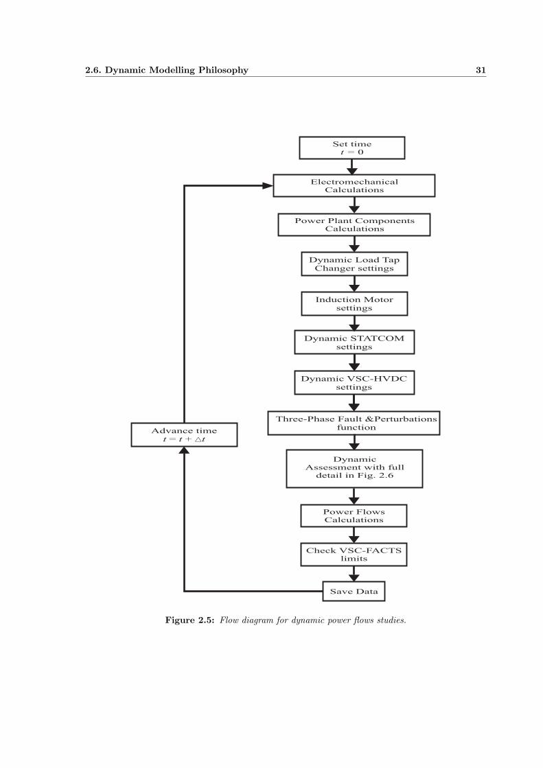
2.6. Dynamic Modelling Philosophy 31
Electromechanical
Calculations
Dynamic Load Tap
Changer settings
Power Plant Components
Calculations
Dynamic
Assessment with full
detail in Fig. 2.6
Power Flows
Calculations
Advance time
= +t t tD
Three-Phase Fault &Perturbations
function
Dynamic STATCOM
settings
Dynamic VSC-HVDC
settings
Check VSC-FACTS
limits
Save Data
Set time
0t =
Induction Motor
settings
Figure 2.5: Flow diagram for dynamic power flows studies.
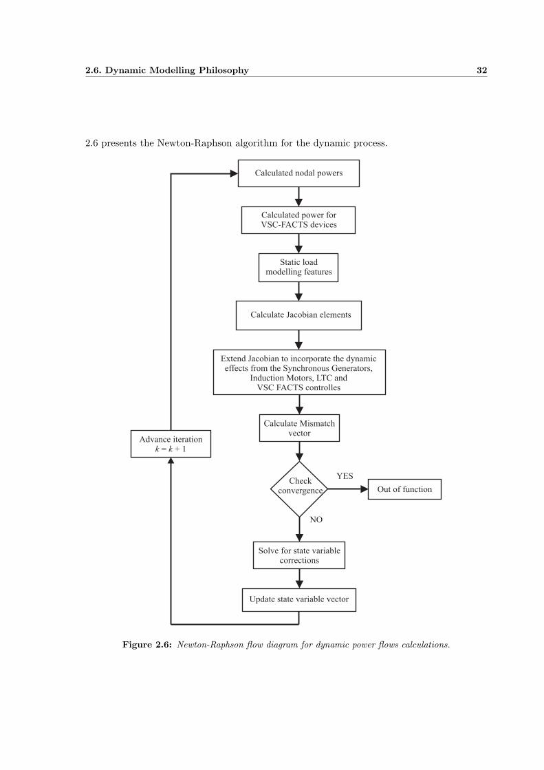
2.6. Dynamic Modelling Philosophy 32
2.6 presents the Newton-Raphson algorithm for the dynamic process.
Calculated nodal powers
Calculated power for
VSC-FACTS devices
Calculate Jacobian elements
Extend Jacobian to incorporate the dynamic
effects from the Synchronous Generators,
Induction Motors, LTC and
VSC FACTS controlles
Check
convergence
YES
Calculate Mismatch
vector
Solve for state variable
corrections
Out of function
Update state variable vector
Advance iteration
= + 1k k
Static load
modelling features
NO
Figure 2.6: Newton-Raphson flow diagram for dynamic power flows calculations.
2.7. The Trapezoidal Method 33
2.7 The Trapezoidal Method
Prior to the advent of digital computers only a few methods of solving ordinary differential
equations (ODEs) were practical. Hand calculation precluded the use of complex formulae
and also made large system studies impossible.
Since then, numerical analyses has become very important, not only to the mathemati-
cians but also to the scientists and engineers. Each problem requires special consideration
in order to get the best available solution method. This is specially true in the solution of
ODEs where the choice of method can make the difference between good and bad results.
The stability of a method for the solution of ODEs is of great importance and has received
a great deal of attention [Gear, 1971b, Gear, 1971a, Lapidus and Seinfeld, 1971, Williams,
1972]. The implicit trapezoidal integration method has been used as a method of solving
the multi-machine transient stability problem [Dommel and Sato, 1972], and has gained
recognition as a very powerful method, having great advantages over the more traditional
methods such as Gauss, Gauss-Seidel, Runge-Kutta and Euler.
The trapezoidal method is derived from the general multi-step equation,
k∑
i=0
αi yn−i+1 + hk∑
i=0
βi yn−i+1 = 0 (2.9)
where αi and βi are constant, and with k equal to unity it becomes a single step method.
The solution at the end of n + 1 steps is given by:
yn+1 = yn +hn+1
2(yn+1 + yn) (2.10)
This is implicit and requires an iterative solution. The solution can be made directly if
the derivative can be replaced by the differential equations, forming an algebraic equation.
The accuracy of the method may be determined by expanding each term in Eq. 2.9 by a
Taylor’s series. The lowest non-zero coefficient is for y(3)n and is − 1
12h3. Thus the trapezoidal
2.7. The Trapezoidal Method 34
method has second order accuracy and the true solution may be given as:
y(xn+1) = yn +h
2
(y
(1)n+1 + y(1)
n
)+ 0(h3) + εn+1 (2.11)
where εn+1 represents the round-off error at the n + 1th step.
The characteristic root of the method when applied to the ordinary differential equations
is,
y = λy (2.12)
with y(0) = y0 is
z1 = (1− 2bn+1) (2.13)
where
bn+1 =hn+1(
hn+1 − 2λ
) (2.14)
If <(λ) < 0 then 0 ≤ bn+1 ≤ 1 and |z1| ≤ 1. The trapezoidal method is therefore A-stable.
This means that the method has an infinite stability boundary (unconditionally stable). The
trapezoidal method is linear and thus in a multi-variable problem, like the power system
stability problem, the method is sigma-stable (multi-variable version of A-stability). The
two are equivalent when the method is linear but may not be equivalent otherwise. Back
Euler and the trapezoidal method are sigma-stable, single step methods.
The great advantage of this method is that the solution of all the variables is simultane-
ous. With the more traditional methods, using explicit integration methods, interface errors
occurred due to the out of step solution of the two groups of variables in the problem.
2.8. Summary 35
2.8 Summary
This chapter has outlined the issues of power system dynamics, emphasising current agree-
ment on the classification of power system stability phenomena and its importance in power
plants modelling development. The main tools available for voltage stability assessments
and their main drawbacks compared to the models and algorithms developed in this research
work.
Key concepts regarding dynamic stability studies, focusing on voltage stability assessment,
are described within the context of the current research project. The main requirements for
off-line analyses of electric power networks are assessed. Besides, the great importance of
equipment modelled for voltage stability simulation is remark.
The data modelling which is an issue of noteworthiness for voltage stability studies is
addressed. The definition of contingency for voltage stability studies and the significance of
slow and fast dynamics are described.
The modelling philosophy adopted to tackle the voltage stability problem is described.
The difference between this approach and the conventional techniques to solve the problem
are stated. Moreover, a clear explanation about the integration method used to discretised
the differential equations is introduced.

Chapter 3
Newton-Raphson Power Flow
Algorithm in abc Rectangular
Co-ordinates
3.1 Introduction
Modern system interconnections enable the safe exchange of electric power between re-
gions or countries, taking advantage of load diversity in time and space leading to a more
economical and environmental way of supplying electricity to consumers. The key advantages
of interconnected systems are [Arrillaga et al., 2007]:
1. the pooling of generation capability with the opportunity to utilise diverse primary
energy resources;
2. the creation of larger markets, which enable economies of scale to be realised in the
operation of power plants and in accommodating demand growth;
3. significant flexibility for the introduction of competition into electricity supply.
3.2. Power Flows Concepts 37
Such advantages have been conventionally alighted by the use of additional AC lines
between the various interconnected systems, in order to reinforce the interconnections. Nev-
ertheless, with the increasing complexity of power systems and consumers’ appetite for elec-
tricity, the reliability of power supply has deteriorated, bringing about, as a consequence,
a great number of blackouts in various parts of the world [Knight, 2001]. Consequently,
strengthening the transmission system is vital to the reliability of block power interchanges
among interconnected power systems.
It is argued by HVDC enthusiasts that the probability to decrease blackouts and bottle-
necks in power systems can be substantially alleviated with the use of HVDC interconnection.
The thrust of this chapter is the development and modelling of three-phase power AC-DC
networks making use of the Newton-Raphson method in rectangular co-ordinates.
3.2 Power Flows Concepts
Power flows solutions is the most frequently performed kind of study in power systems
engineering. The power flow formulation is at the heart of power system analyses and is
closely associated with voltage stability analyses [Taylor, 1994].
The classical Newton [Tinney and Hart, 1967] and fast decoupled load flow [Stott and
Alsac, 1974] have been extensively used in power flow analyses for the last decades. The
steady-state conditions relating to transmission systems are obtained by assuming balanced
operation in most cases. However, the proposals and developments of algorithms for three-
phase power flows calculation for unbalanced power system conditions are increasing [Ar-
rillaga and Watson, 2001,Wilsun Xu and Dommel, 1991, Smith and Arrillaga, 1998, Zhang,
1996].
To solve the power flow problem, the most general and reliable algorithm is the Newton-
Raphson method. The basis of this iterative method relies on successive linearization of the
non-linear set of equations that represent the electrical power network using only the first
3.2. Power Flows Concepts 38
term of the Taylor’s series expansion.
The Newton-Raphson method, as applied to the three-phase power flow problem in rect-
angular co-ordinates, is dealt with detail in this chapter.
The Newton-Raphson method in rectangular co-ordinates, as opposed to the one in polar
co-ordinates, is less well-known but it is equally effective and it goes on well with the method
of dynamic power flows which is the central focus of this thesis.
3.2.1 The power flow problem formulation
The main object of the power flow solution is to obtain the nodal phase voltages at all
buses of the network corresponding to specified system level of generation and load patterns.
In power flow analyses using rectangular co-ordinates, the nodal voltages are expressed as
a function of their real and imaginary parts. The complex voltages, expressed as real and
imaginary parts are the state variables rather than the magnitude and phase angles used in
the polar co-ordinate analyses.
As voltage magnitudes and angles are involved, it follows that for each bus, six indepen-
dent constraints are required in order to solve for the six unknowns. These constraints are
different for different types of buses. The two main types are load and generators buses, with
the slack bus being treated as a special case of the generator bus.
Despite the fact that the number of equations and variables involved in the solution of
power flows in rectangular co-ordinates is greater than in polar co-ordinates, when spar-
sity techniques are applied, such an increase in size is of little significance. Each iteration
carried out in rectangular co-ordinates analyses is faster than in polar co-ordinates because
no trigonometric operations are involved [Stagg and El-Abiad, 1968,Arrillaga and Watson,
2001].

3.2. Power Flows Concepts 39
3.2.2 Power flow equations
The power balance equation for a three-phase transmission line component, as shown in
Fig. 3.1, can be written as,
Sa,b,c = P a,b,c + jQa,b,c = V a,b,c(Ia,b,c)∗ (3.1)
where
Sa,b,c is the complex power injected into the three-phase bus.
P a,b,c is the active power injected into the three-phase bus.
Qa,b,c is the reactive power injected into the three-phase bus.
V a,b,c is the voltage at the three-phase bus.
Ia,b,c is the current at the three-phase bus.
with a, b, c referring to the three phases of the system.
In rectangular co-ordinates analyses, the bus voltages and the admittances are expressed
as,
Bus k Bus m
Iak
Ibk
Ick
Iam
Ibm
Icm
Vak
Vbk
Vck
Vam
Vbm
Vcm
Ra
Rb
Rc
La
Lb
Lc
Ca C
a
Cb
Cc
Cb
Cc
}}
Lab
Lbc
Lac
Figure 3.1: Three-phase transmission line diagram.

3.2. Power Flows Concepts 40
V ρk =
ebk + jf b
k
ebk + jf b
k
eck + jf c
k
(3.2)
and
Y ρρkm =
Y aakm Y ab
km Y ackm
Y bakm Y bb
km Y bckm
Y cakm Y cb
km Y cckm
=
Gaakm + jBaa
km Gabkm + jBab
km Gackm + jBac
km
Gbakm + jBba
km Gbbkm + jBbb
km Gbckm + jBbc
km
Gcakm + jBca
km Gcbkm + jBcb
km Gcckm + jBcc
km
(3.3)
Separating the real and imaginary parts of Eq. 3.1, in expanded form, leads to nodal
active and reactive power expressions for phase ρ,
Pkρ = eρ
k
∑
i=k,m
∑
j=a,b,c
(Gρj
kieji −Bρj
ki fji
)+ fρ
k
∑
i=k,m
∑
j=a,b,c
(Gρj
kifji + Bρj
ki eji
)(3.4)
Qkρ = fρ
k
∑
i=k,m
∑
j=a,b,c
(Gρj
kieji −Bρj
ki fji
)− eρ
k
∑
i=k,m
∑
j=a,b,c
(Gρj
kifji + Bρj
ki eji
)(3.5)
where ρ is used to denote phases a, b and c. Expressions for the active and reactive power
injected at node m are similar in form with subscript m replacing k and viceversa.
3.2.3 The Jacobian matrix formation
The linearised three-phase power flow expression using rectangular co-ordinates is con-
structed using the real and imaginary parts of the voltage to form the Jacobian matrix and
the mismatch voltages vector.
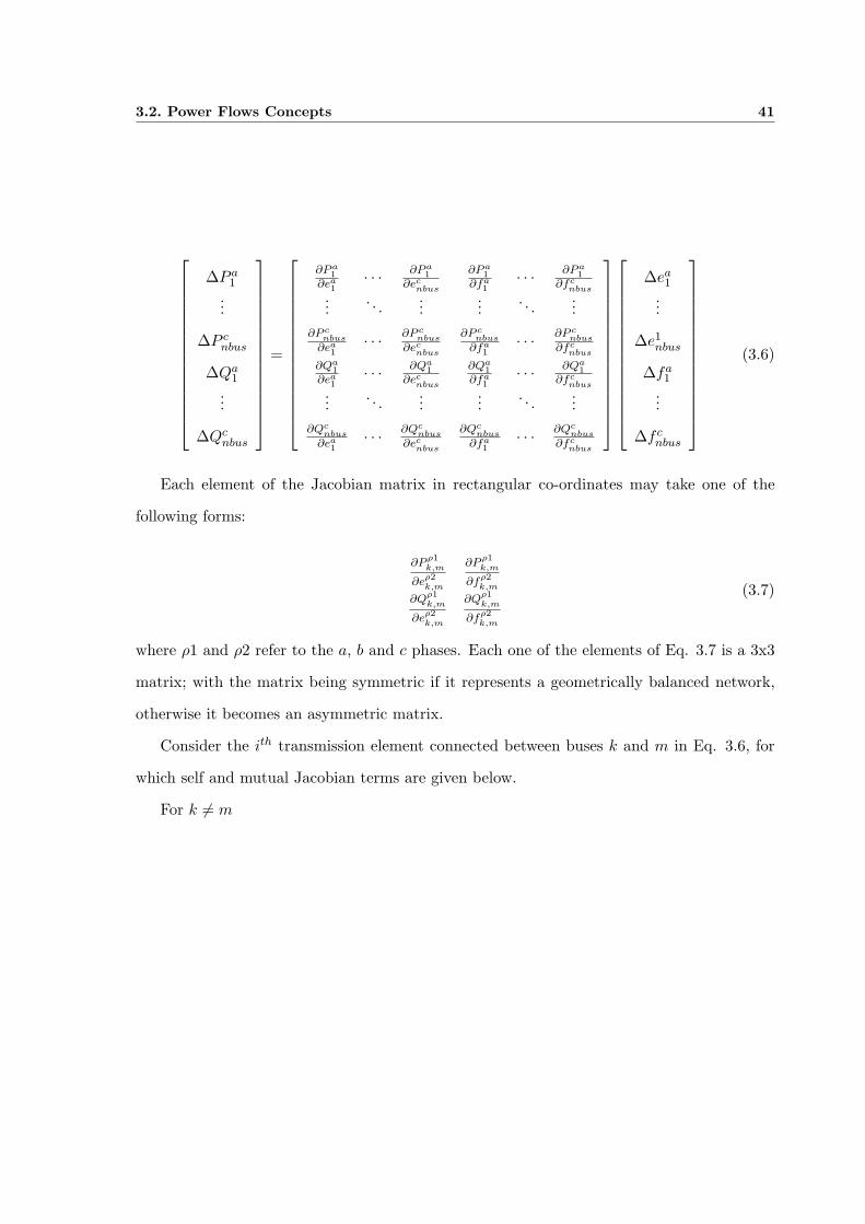
3.2. Power Flows Concepts 41
∆P a1
...
∆P cnbus
∆Qa1
...
∆Qcnbus
=
∂P a1
∂ea1
· · · ∂P a1
∂ecnbus
∂P a1
∂fa1
· · · ∂P a1
∂fcnbus
.... . .
......
. . ....
∂P cnbus
∂ea1
· · · ∂P cnbus
∂ecnbus
∂P cnbus
∂fa1
· · · ∂P cnbus
∂fcnbus
∂Qa1
∂ea1
· · · ∂Qa1
∂ecnbus
∂Qa1
∂fa1
· · · ∂Qa1
∂fcnbus
.... . .
......
. . ....
∂Qcnbus
∂ea1
· · · ∂Qcnbus
∂ecnbus
∂Qcnbus
∂fa1
· · · ∂Qcnbus
∂fcnbus
∆ea1
...
∆e1nbus
∆fa1
...
∆f cnbus
(3.6)
Each element of the Jacobian matrix in rectangular co-ordinates may take one of the
following forms:
∂P ρ1k,m
∂eρ2k,m
∂P ρ1k,m
∂fρ2k,m
∂Qρ1k,m
∂eρ2k,m
∂Qρ1k,m
∂fρ2k,m
(3.7)
where ρ1 and ρ2 refer to the a, b and c phases. Each one of the elements of Eq. 3.7 is a 3x3
matrix; with the matrix being symmetric if it represents a geometrically balanced network,
otherwise it becomes an asymmetric matrix.
Consider the ith transmission element connected between buses k and m in Eq. 3.6, for
which self and mutual Jacobian terms are given below.
For k 6= m
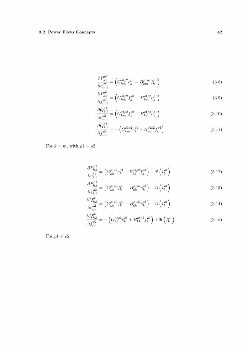
3.2. Power Flows Concepts 42
∂P ρ1k,i
∂eρ2m,i
=(Gρ1ρ2
km eρ1k + Bρ1ρ2
km fρ1k
)(3.8)
∂P ρ1k,i
∂fρ2m,i
=(Gρ1ρ2
km fρ1k −Bρ1ρ2
km eρ1k
)(3.9)
∂Qρ1k,i
∂eρ2m,i
=(Gρ1ρ2
km fρ1k −Bρ1ρ2
km eρ1k
)(3.10)
∂Qρ1k,i
∂fρ2m,i
= −(Gρ1ρ2
km eρ1k + Bρ1ρ2
km fρ1k
)(3.11)
For k = m, with ρ1 = ρ2
∂P ρ1k,i
∂eρ2k,i
=(Gρ1ρ2
kk eρ1k + Bρ1ρ2
kk fρ1k
)+ <
(Iρ1k
)(3.12)
∂P ρ1k,i
∂fρ2k,i
=(Gρ1ρ2
kk fρ1k −Bρ1ρ2
kk eρ1k
)+ =
(Iρ1k
)(3.13)
∂Qρ1k,i
∂eρ2k,i
=(Gρ1ρ2
kk fρ1k −Bρ1ρ2
kk eρ1k
)−=
(Iρ1k
)(3.14)
∂Qρ1k,i
∂fρ2k,i
= −(Gρ1ρ2
kk eρ1k + Bρ1ρ2
kk fρ1k
)+ <
(Iρ1k
)(3.15)
For ρ1 6= ρ2

3.2. Power Flows Concepts 43
∂P ρ1k,i
∂eρ2k,i
=(Gρ1ρ2
kk eρ1k + Bρ1ρ2
kk fρ1k
)(3.16)
∂P ρ1k,i
∂fρ2k,i
=(Gρ1ρ2
kk fρ1k −Bρ1ρ2
kk eρ1k
)(3.17)
∂Qρ1k,i
∂eρ2k,i
=(Gρ1ρ2
kk fρ1k −Bρ1ρ2
kk eρ1k
)(3.18)
∂Qρ1k,i
∂fρ2k,i
= −(Gρ1ρ2
kk eρ1k + Bρ1ρ2
kk fρ1k
)(3.19)
where the current Iρ1i,j is:
Iρ1k,i =
∑
l=k,m
∑
ρ2=a,b,c
[(Gρ1ρ2
kl eρ2l −Bρ1ρ2
kl fρ2l
)+ j
(Bρ1ρ2
kl eρ2l + Gρ1ρ2
kl fρ1l
)](3.20)
The Jacobian matrix and mismatch vector are evaluated at each iteration. The generic
power mismatch equations at bus k are:
∆P ρk,m =
(P ρ
k,m
)sp−
(P ρ
k,m
)cal,it(3.21)
∆Qρk,m =
(Qρ
k,m
)sp−
(Qρ
k,m
)cal,it(3.22)
where(P ρ
k,m
)spand
(Qρ
k,m
)spare the specified active and reactive power injections deter-
mined by the net amount of power generation and load connected to the bus, and(P ρ
k,m
)cal,it
and(Qρ
k,m
)cal,itare the calculated active and reactive injections at the bus using the corre-
sponding nodal voltages, (eρ + jfρ)it. Normally, the nodal voltage for phase a is initialised
at one and zero for real and imaginary part, respectively, while phases b and c are initialised
at −12 − j
√3
2 and −12 + j
√3
2 respectively. At each iteration the nodal voltages are updated

3.2. Power Flows Concepts 44
according to the following expression.
(eρ + jfρ)it+1 =[(
eρk
)it +(∆eρ
k
)it]
+ j[(
fρk
)it +(∆fρ
k
)it]
(3.23)
The process is repeated until the complex power mismatches are within a specified toler-
ance, e.g. 1e− 12.
3.2.4 Voltage controlled bus
In the Newton-Raphson method using rectangular co-ordinates, a nodal voltage magni-
tude mismatch equation is needed for each PV-type bus [Stagg and El-Abiad, 1968]. The
equation for a voltage-controlled bus become,
P ρ1k =
nbus∑
m=1
[eρ1k
(Gρ1ρ2
km eρ2m −Bρ1ρ2
km fρ2m
)+ fρ1
m
(Gρ1ρ2
km fρ2m + Bρ1ρ2
km eρ2m
)](3.24)
(V ρ1
k
)2=
(eρ1k
)2+
(fρ1
k
)2(3.25)
Accordingly, new types of Jacobian elements are needed for the Jacobian matrix in rect-
angular co-ordinates where:
∂(V ρ1
k,m
)2
∂eρ2k,m
(3.26)
and
∂(V ρ1
k,m
)2
∂fρ2k,m
(3.27)
For the ith element connected to a PV-type bus, say k, the Jacobian elements are:

3.3. Power System Loads 45
∂(V ρ1
k,i
)2
∂eρ2k,i
= 2eρk,i (3.28)
∂(V ρ1
k,i
)2
∂fρ2k,i
= 2fρk,i (3.29)
∂(V ρ1
k,i
)2
∂eρ2m,i
= 0 (3.30)
∂(V ρ1
k,i
)2
∂fρ2m,i
= 0 (3.31)
Changes in voltage magnitude for the RV-type buses at iteration it are calculated as
follows:
∆[(
V ρk
)2]i
t =[(
V ρk(scheduled)
)]it−
[(V ρ
k
)2]i
t (3.32)
At iteration it the reactive power at each voltage controlled bus is reviewed using Eq. 3.5
to calculate reactive power and to check its limits. If the source of reactive power exceeds the
limits the bus changes to a load bus with fixed reactive power, equal to the violated limit.
The process is repeated until complex power mismatches are within a specified tolerance,
e.g. 1e− 12.
Fig. 3.2 depicts the flow diagram for three-phase power flows using the Newton-Raphson
method in rectangular co-ordinates.
3.3 Power System Loads
Load modelling has a significant influence on power systems operation, simulation and
analyses. Usually, the power system loads are modelled as constant three-phase power sink,
which can be connected either in an star or delta arrangement [Chen and Dillon, 1974],
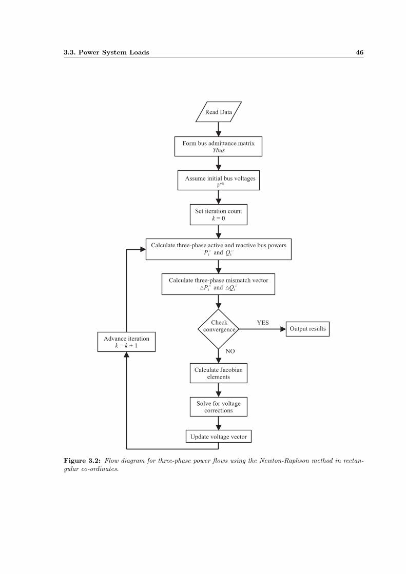
3.3. Power System Loads 46
Read Data
Form bus admittance matrix
Ybus
Set iteration count
= 0k
Assume initial bus voltages
V(0)
Calculate three-phase active and reactive bus powers
andPk
r
Qk
r
Calculate three-phase mismatch vector
andD DPk
r
Qk
r
Check
convergence
YES
Calculate Jacobian
elements
Solve for voltage
corrections
Output results
Update voltage vector
Advance iteration
= + 1k k
NO
Figure 3.2: Flow diagram for three-phase power flows using the Newton-Raphson method in rectan-gular co-ordinates.

3.3. Power System Loads 47
Sρl = P ρ
l + jQρl (3.33)
where Pl and Ql are the active and reactive load powers; a, b and c are phases of the load
system represented by the superscript ρ.
However, this kind of model is inadequate for some power system studies such as dynamic
and voltage collapse studies.
Temporary the unbalance between the power generation and the power demand reduce
systems security margins and increase the risks unsafe operation. In order to reduce such risks,
system studies have to be carried out with more realistic models for all systems components,
including load models.
A very substantial part of the system load actually consists of induction motors. Hence,
if data is available induction motor modelling must be considered and carry out.
For power system analyses, the load is refer as the active and reactive power delivered to
specific buses of the network at subtransmission and distribution level.
In spite of the fact, that it very simple to model certain types of loads, usually it is very
difficult to find the exact composition of the load. In common practice, the load is modelled
as (a) constant power, (b) constant current and (c) constant impedance, and sometimes it is
modelled as a combination of (a), (b) and (c).
Normally the load power varies with respect to the voltage and frequency. The effect of
voltage angle on reactive load power is zero whilst its effect on the active load power is of a
transient nature which persists for less than a second [IEEE Working Group on Power Plant
Response to Load Changes, 1973].
The mathematical load model that includes the effect of the voltage magnitude may be
approximated by
S = P0
( |V ||V0|
)n
+ jQ0
( |V ||V0|
)m
(3.34)
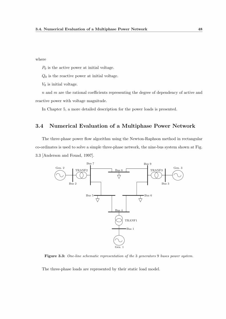
3.4. Numerical Evaluation of a Multiphase Power Network 48
where
P0 is the active power at initial voltage.
Q0 is the reactive power at initial voltage.
V0 is initial voltage.
n and m are the rational coefficients representing the degree of dependency of active and
reactive power with voltage magnitude.
In Chapter 5, a more detailed description for the power loads is presented.
3.4 Numerical Evaluation of a Multiphase Power Network
The three-phase power flow algorithm using the Newton-Raphson method in rectangular
co-ordinates is used to solve a simple three-phase network, the nine-bus system shown at Fig.
3.3 [Anderson and Fouad, 1997].
Bus 1
Bus 2 Bus 3
Bus 4
Bus 5 Bus 6
Bus 7
Bus 8
Bus 9
Gen. 2 Gen. 3
Gen. 1
TRANF1
TRANF2 TRANF3
Figure 3.3: One-line schematic representation of the 3 generators 9 buses power system.
The three-phase loads are represented by their static load model.
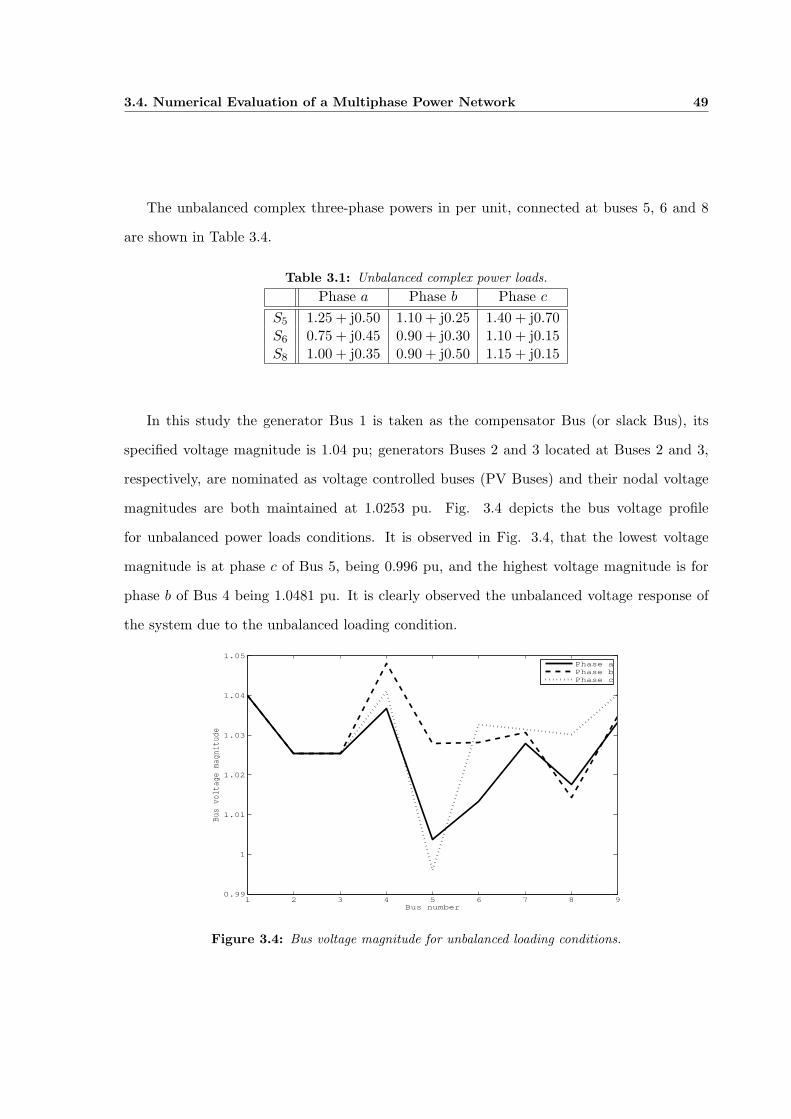
3.4. Numerical Evaluation of a Multiphase Power Network 49
The unbalanced complex three-phase powers in per unit, connected at buses 5, 6 and 8
are shown in Table 3.4.
Table 3.1: Unbalanced complex power loads.Phase a Phase b Phase c
S5 1.25 + j0.50 1.10 + j0.25 1.40 + j0.70S6 0.75 + j0.45 0.90 + j0.30 1.10 + j0.15S8 1.00 + j0.35 0.90 + j0.50 1.15 + j0.15
In this study the generator Bus 1 is taken as the compensator Bus (or slack Bus), its
specified voltage magnitude is 1.04 pu; generators Buses 2 and 3 located at Buses 2 and 3,
respectively, are nominated as voltage controlled buses (PV Buses) and their nodal voltage
magnitudes are both maintained at 1.0253 pu. Fig. 3.4 depicts the bus voltage profile
for unbalanced power loads conditions. It is observed in Fig. 3.4, that the lowest voltage
magnitude is at phase c of Bus 5, being 0.996 pu, and the highest voltage magnitude is for
phase b of Bus 4 being 1.0481 pu. It is clearly observed the unbalanced voltage response of
the system due to the unbalanced loading condition.
1 2 3 4 5 6 7 8 90.99
1
1.01
1.02
1.03
1.04
1.05
Bus number
Bus
volt
age
magn
itud
e
Phase aPhase bPhase c
Figure 3.4: Bus voltage magnitude for unbalanced loading conditions.
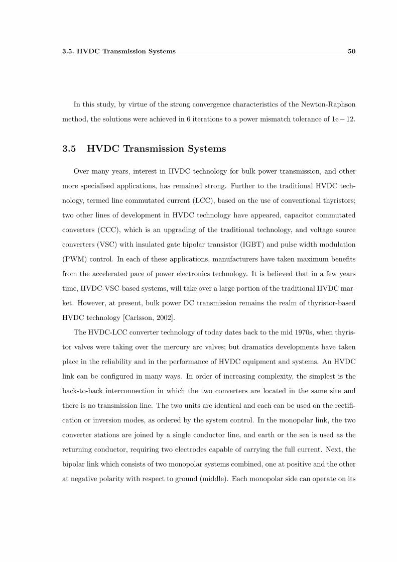
3.5. HVDC Transmission Systems 50
In this study, by virtue of the strong convergence characteristics of the Newton-Raphson
method, the solutions were achieved in 6 iterations to a power mismatch tolerance of 1e−12.
3.5 HVDC Transmission Systems
Over many years, interest in HVDC technology for bulk power transmission, and other
more specialised applications, has remained strong. Further to the traditional HVDC tech-
nology, termed line commutated current (LCC), based on the use of conventional thyristors;
two other lines of development in HVDC technology have appeared, capacitor commutated
converters (CCC), which is an upgrading of the traditional technology, and voltage source
converters (VSC) with insulated gate bipolar transistor (IGBT) and pulse width modulation
(PWM) control. In each of these applications, manufacturers have taken maximum benefits
from the accelerated pace of power electronics technology. It is believed that in a few years
time, HVDC-VSC-based systems, will take over a large portion of the traditional HVDC mar-
ket. However, at present, bulk power DC transmission remains the realm of thyristor-based
HVDC technology [Carlsson, 2002].
The HVDC-LCC converter technology of today dates back to the mid 1970s, when thyris-
tor valves were taking over the mercury arc valves; but dramatics developments have taken
place in the reliability and in the performance of HVDC equipment and systems. An HVDC
link can be configured in many ways. In order of increasing complexity, the simplest is the
back-to-back interconnection in which the two converters are located in the same site and
there is no transmission line. The two units are identical and each can be used on the rectifi-
cation or inversion modes, as ordered by the system control. In the monopolar link, the two
converter stations are joined by a single conductor line, and earth or the sea is used as the
returning conductor, requiring two electrodes capable of carrying the full current. Next, the
bipolar link which consists of two monopolar systems combined, one at positive and the other
at negative polarity with respect to ground (middle). Each monopolar side can operate on its

3.5. HVDC Transmission Systems 51
own with ground return, but if the two poles have equal currents, they cancel out each other’s
ground current to practically zero. In such cases, the ground path is used for limited periods
in emergency, when one pole is temporarily out of service. Other more complex configurations
are possible such as multiterminal links and series connections. The central components of
any HVDC-LCC converter are the thyristor valves, used to perform the conversion from AC
to DC and vice versa. The thyristor valves are made of highly pure monocrystalline silicon.
The high performance thyristors installed in HVDC plants today are characterized by silicon
wafer diameters of up to 125 mm, blocking voltages up to 8kV and current carrying capacities
of up to 4kA DC [Siemens AG Power Transmission and Distribution High Voltage Division,
2007].
The converter stations are connected to the AC busbars by means of converter trans-
former, which scale-down the voltage of the grid to the required entry voltage of the converter.
The converter transformer is equipped with an on-load tap changer.
A large inductance (smoothing reactor) is installed on the DC side current to prevent
resonance in the DC circuit, to reduce the ripple in the direct current and to limit telephone
interference. In addition, a DC filter is needed to reduce the level of harmonic currents in
the DC overhead line.
On the AC side, harmonics current are prevented from entering the AC network by using
AC filters, i.e. resonant circuits comprising capacitors, reactors and resistors. The reac-
tive power consumption of an HVDC converter is a function of active power, transformer
reactances and control angle. It increases with increasing active power. Full reactive power
compensation is a standard requirement in a converter station; with part of the reactive power
produced by filters and the rest by shunt capacitor banks or synchronous condensers when dy-
namic compensating is deemed necessary [Siemens AG Power Transmission and Distribution
High Voltage Division, 2007].
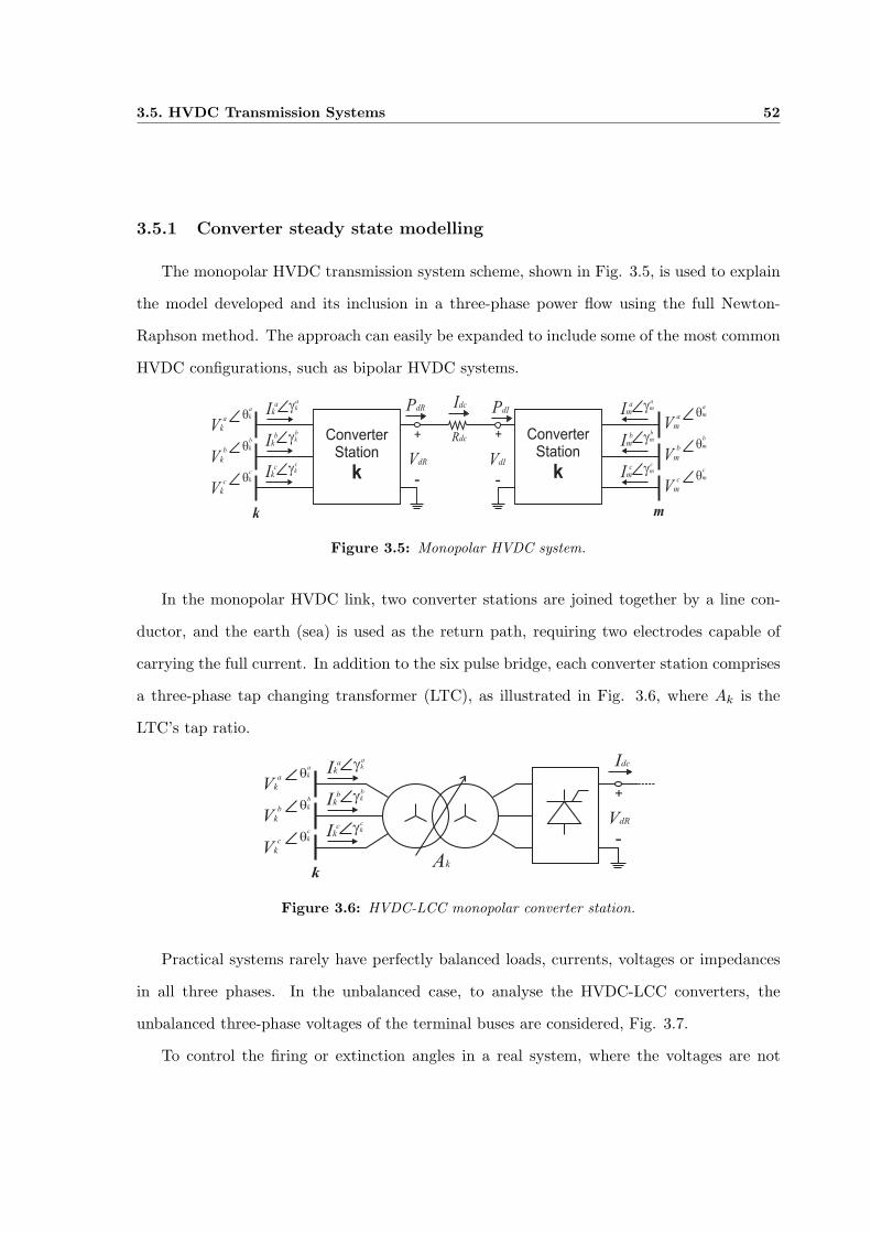
3.5. HVDC Transmission Systems 52
3.5.1 Converter steady state modelling
The monopolar HVDC transmission system scheme, shown in Fig. 3.5, is used to explain
the model developed and its inclusion in a three-phase power flow using the full Newton-
Raphson method. The approach can easily be expanded to include some of the most common
HVDC configurations, such as bipolar HVDC systems.
Vk
qk
k
VdR
+
-VdI
+
-
Rdc
IdcPdR PdIa
a
Vk
qk
b
b
Vk
qk
c
c
Ikgk
aa
Ikgk
bb
Ikgk
cc
m
Vm
qm
a
a
Vm
qm
b
b
Vm
qm
c
c
Imgm
aa
Imgm
bb
Imgm
cc
ConverterStation
k
ConverterStation
k
Figure 3.5: Monopolar HVDC system.
In the monopolar HVDC link, two converter stations are joined together by a line con-
ductor, and the earth (sea) is used as the return path, requiring two electrodes capable of
carrying the full current. In addition to the six pulse bridge, each converter station comprises
a three-phase tap changing transformer (LTC), as illustrated in Fig. 3.6, where Ak is the
LTC’s tap ratio.
Vk
qk
kAk
VdR
+
-
Idca
a
Vk
qk
b
b
Vk
qk
c
c
Ikgk
aa
Ikgk
bb
Ikgk
cc
Figure 3.6: HVDC-LCC monopolar converter station.
Practical systems rarely have perfectly balanced loads, currents, voltages or impedances
in all three phases. In the unbalanced case, to analyse the HVDC-LCC converters, the
unbalanced three-phase voltages of the terminal buses are considered, Fig. 3.7.
To control the firing or extinction angles in a real system, where the voltages are not
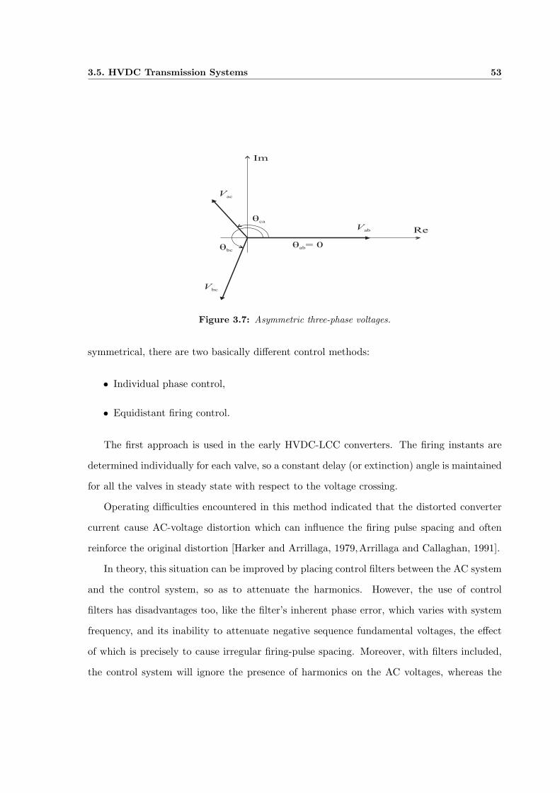
3.5. HVDC Transmission Systems 53
Re
Im
Vac
Vab
Vbc
qca
qab= 0q
bc
Figure 3.7: Asymmetric three-phase voltages.
symmetrical, there are two basically different control methods:
• Individual phase control,
• Equidistant firing control.
The first approach is used in the early HVDC-LCC converters. The firing instants are
determined individually for each valve, so a constant delay (or extinction) angle is maintained
for all the valves in steady state with respect to the voltage crossing.
Operating difficulties encountered in this method indicated that the distorted converter
current cause AC-voltage distortion which can influence the firing pulse spacing and often
reinforce the original distortion [Harker and Arrillaga, 1979,Arrillaga and Callaghan, 1991].
In theory, this situation can be improved by placing control filters between the AC system
and the control system, so as to attenuate the harmonics. However, the use of control
filters has disadvantages too, like the filter’s inherent phase error, which varies with system
frequency, and its inability to attenuate negative sequence fundamental voltages, the effect
of which is precisely to cause irregular firing-pulse spacing. Moreover, with filters included,
the control system will ignore the presence of harmonics on the AC voltages, whereas the
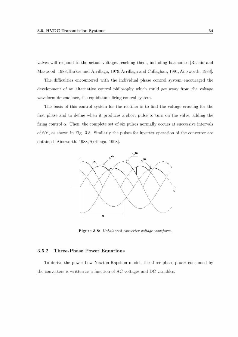
3.5. HVDC Transmission Systems 54
valves will respond to the actual voltages reaching them, including harmonics [Rashid and
Maswood, 1988,Harker and Arrillaga, 1979,Arrillaga and Callaghan, 1991,Ainsworth, 1988].
The difficulties encountered with the individual phase control system encouraged the
development of an alternative control philosophy which could get away from the voltage
waveform dependence, the equidistant firing control system.
The basis of this control system for the rectifier is to find the voltage crossing for the
first phase and to define when it produces a short pulse to turn on the valve, adding the
firing control α. Then, the complete set of six pulses normally occurs at successive intervals
of 60◦, as shown in Fig. 3.8. Similarly the pulses for inverter operation of the converter are
obtained [Ainsworth, 1988,Arrillaga, 1998].
Figure 3.8: Unbalanced converter voltage waveform.
3.5.2 Three-Phase Power Equations
To derive the power flow Newton-Rapshon model, the three-phase power consumed by
the converters is written as a function of AC voltages and DC variables.
3.5. HVDC Transmission Systems 55
P ρk = f
(V a,b,c
k , θa,b,ck , X
)(3.35)
P ρm = f
(V a,b,c
m , θa,b,cm , X
)(3.36)
where Pk and Pm are active powers at buses k and m, respectively; Vk and θk and Vm and
θm are the voltage magnitudes and phase angles, respectively, at the sending and receiving
buses k and m; ρ denotes the a, b, and c phases of the system. X represents, in generic form
at this stage, the DC variables.
The reactive powers are,
Qρk =
√(Sρ
k)2 − (P ρk )2 =
√(k1AkV
ρk Idc
)2
3− (P ρ
k )2 (3.37)
Qρm =
√(Sρ
m)2 − (P ρm)2 =
√(k1AmV ρ
mIdc)2
3− (P ρ
m)2 (3.38)
where Sk, Sm and Qk, Qm are the complex and reactive powers at buses k and m respectively;
k1 is a constant associated with the commutation overlap, Ak and Am are the tap changers
positions at buses k and m, respectively; and Idc is the current in the dc-link. The full
derivation is given in Appendix A.
3.5.3 Linearised power equations
A three-phase power network with n-buses is described by 6×(n−1) non linear equations.
The inclusion of one HVDC link in the network model augments the number of equations by
six. The solution of the combined system of non-linear equations is carried out by iteration
using the full Newton-Raphson method.
The power through the dc-link can be controlled by varying the DC-voltages as indicated
3.5. HVDC Transmission Systems 56
by the following two basic relations:
PdR = VdRIdc (3.39)
PdI = VdIIdc (3.40)
where PdR and PdI are the DC powers at the inverter and rectifier ends, respectively; and
VdR and VdI are the DC voltages, at the rectifier and inverter, respectively.
The DC-voltages can be controlled either with the transformers tap ratios or with the
converters control angles. At the rectifier, the control angle is the firing angle α; and at the
inverter, the control angle is the extinction angle, γ. An increase in the control angle gives
a decrease in DC-voltage, an increase in reactive power consumption (since the current will
lag the voltage) and an increase in harmonics generation. The latter is clearly undesirable
and there is thus some benefit in keeping the control angles at low values [Arrillaga, 1998].
There are several modes of operation in converter control. The first one, when the firing
angle α, the extinction angle γ, VdI and PdI are specified, is called control mode A. The
converter transformer taps are varied in order to meet these specifications. In control mode
B, the extinction angle γ, is kept at its lower limit at the inverter and the transformer taps
and the power PdI are specified. The power is controlled by varying the firing angle α at the
rectifier. The firing angle rather than the tap transformer is preferred for control, since the
tap changer control is too slow compared to the firing angle. In control mode C, α is fixed
to its minimum value and γ is regulated to maintain constant power.
If the current Idc is kept constant instead of the power PdI , three other control modes are
defined. In this paper only the mode A, B and C with constant power are addressed.
The Jacobian used in conventional power flows is suitably extended to take account of
the new elements contributed by the HVDC link. The set of linearised power flow equations
for the complete system is,
3.5. HVDC Transmission Systems 57
∆P
∆Q
−−∆PdR
∆PdI
=
J11 | J12
−− + −−J21 | J22
∆θ
∆VV
−−∆X1
∆X2
(3.41)
where
∆P = [∆P ρ1 , · · · ,∆P ρ
n ]t
∆Q = [∆Qρ1, · · · ,∆Qρ
n]t
∆θ = [∆θρ1, · · · , ∆θρ
n]t
∆VV =
[∆V ρ
1
V ρ1
, · · · , ∆V ρn
V ρn
]t
∆P and ∆Q are the normal power mismatch equations, and ∆θ and ∆VV are voltage
increments of phase angle and magnitude, respectively.
There are two additional state variables X1 and X2, (i.e. X1,2), and two power mismatch
equations introduced by the HVDC link,
∆PdR = P schdR − P cal
dR (3.42)
∆PdI = P schdI − P cal
dI (3.43)
P sch and P cal are the scheduled and calculated powers for the HVDC link.
The power mismatches for buses k and m, where the HVDC link is connected to become:
3.5. HVDC Transmission Systems 58
∆Pk = PGk − PLk − PNk (θ, V )− PdR (Vk, Vm, X1,2) (3.44)
∆Pm = PGm − PLm − PNm (θ, V )− PdI (Vk, Vm, X1,2) (3.45)
∆Qk = QGk −QLk −QNk (θ, V )−QdR (Vk, Vm, X1,2) (3.46)
∆Qm = QGm −QLm −QNm (θ, V )−QdI (Vk, Vm, X1,2) (3.47)
where PGk, QGk and PGm and QGm represent the active and reactive powers injected by the
generator at buses k and m, respectively; PLk, QLk and PLm and QLm represent the active
and reactive powers drawn by the load at buses k and m, respectively;
The J11 matrix corresponding to the AC network at buses k and m
∂P ρk
∂θρk
∂P ρk
∂V ρk
V ρk
∂P ρk
∂θρm
∂P ρk
∂V ρm
V ρm
∂Qρk
∂θρk
∂Qρk
∂V ρk
V ρk
∂Qρk
∂θρm
∂Qρk
∂V ρm
V ρm
∂P ρm
∂θρk
∂P ρm
∂V ρk
V ρk
∂P ρm
∂θρm
∂P ρm
∂V ρm
V ρm
∂Qρm
∂θρk
∂Qρm
∂V ρk
V ρk
∂Qρm
∂θρm
∂Qρm
∂V ρm
V ρm
(3.48)
is augmented with the partial derivatives of the active and reactive powers contributions
by the HVDC link.
Matrix J12 includes the partial derivatives of the three-phase powers P ρk,m and Qρ
m,n with
respect to the HVDC link state variables and J21 represents the partial derivatives of PdR and
PdI with respect to the three-phase voltage angles and magnitudes θρk,m and V ρ
k,m. Moreover,
J22 represents the self partial derivatives of the HVDC link.
3.5.4 Control mode A
In control mode A, the variables α, γ, VdI and PdI are specified, making it possible to
calculate the current Idc, the voltage VdI and the power PdR:
3.5. HVDC Transmission Systems 59
Idc =PdI
VdI(3.49)
VdR = VdI + RDCIdc (3.50)
PdR = VdRIdc (3.51)
The new state variables for this control mode are the tap changers, Ak and Am, with the
Jacobian elements J12, J21 and J22 having the following structure:
J12 =
∂P ρk
∂Ak
∂P ρk
∂Am
∂Qρk
∂Ak
∂Qρk
∂Am
∂P ρm
∂Ak
∂P ρm
∂Am
∂Qρm
∂Ak
∂Qρm
∂Am
(3.52)
J21 =
∂PdR
∂θρk
∂PdR
∂V ρk
V ρk
∂PdR
∂θρm
∂PdR
∂θρm
V ρm
∂PdI
∂θρk
∂PdI
∂V ρk
V ρk
∂PdI
∂θρm
∂PdI
∂θρm
V ρm
(3.53)
J22 =
∂PdR∂Ak
∂PdR∂Am
∂PdI∂Ak
∂PdI∂Am
(3.54)
It should be noted that a single tap changer is used to regulate voltage magnitude at all
three phases.
3.5.5 Control mode B
In control mode B, the variables ak, am, γ and PdI are specified and the new state variables
are the current Idc and the firing angle α. For this control mode, J21 has the same structure
as in control mode A. The other two terms of the Jacobian are:
3.5. HVDC Transmission Systems 60
J12 =
∂P ρk
∂α
∂P ρk
∂Idc
∂Qρk
∂α
∂Qρk
∂Idc
∂P ρm
∂α∂P ρ
m∂Idc
∂Qρm
∂α∂Qρ
m∂Idc
(3.55)
J22 =
∂PdR∂α
∂PdR∂Idc
∂PdI∂α
∂PdI∂Idc
(3.56)
3.5.6 Control mode C
In control mode C, the variables ak, am, α and PdI are specified and the new state
variables are the current Idc and the extinction angle γ. Matrix J21 has the same structure
as in the previous control modes, whereas matrices J12 and J22 take the following structure,
J12 =
∂P ρk
∂Idc
∂P ρk
∂γ
∂Qρk
∂Idc
∂Qρk
∂γ
∂P ρm
∂Idc
∂P ρm
∂γ
∂Qρm
∂Idc
∂Qρm
∂γ
(3.57)
J22 =
∂PdR∂Idc
∂PdR∂γ
∂PdI∂Idc
∂PdI∂γ
(3.58)
It is important to remark that this is a three-phase formulation, and that all elements in
the above equations are vectors of order 3×1, except for J11 which are vectors of order 3×3
and J22 which are single terms.
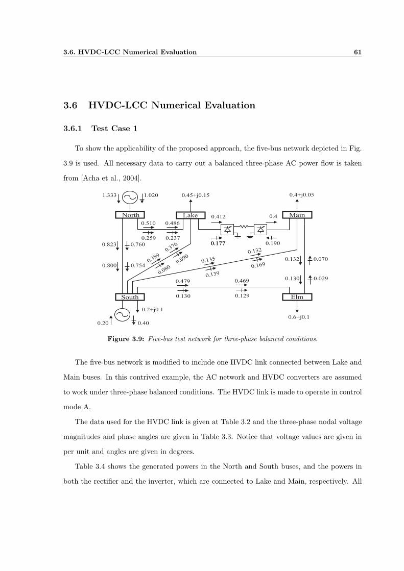
3.6. HVDC-LCC Numerical Evaluation 61
3.6 HVDC-LCC Numerical Evaluation
3.6.1 Test Case 1
To show the applicability of the proposed approach, the five-bus network depicted in Fig.
3.9 is used. All necessary data to carry out a balanced three-phase AC power flow is taken
from [Acha et al., 2004].
MainLakeNorth
ElmSouth
0.4+j0.050.45+j0.15
0.6+j0.1
0.2+j0.1
0.400.20
1.0201.333
0.412
0.177
0.4
0.190
0.510 0.486
0.177
0.259 0.237
0.823
0.479
0.130
0.469
0.129
0.135
0.139
0.132
0.169
0.760
0.800 0.754
0.132 0.070
0.130 0.029
0.376
0.090
0.389
0.080
Figure 3.9: Five-bus test network for three-phase balanced conditions.
The five-bus network is modified to include one HVDC link connected between Lake and
Main buses. In this contrived example, the AC network and HVDC converters are assumed
to work under three-phase balanced conditions. The HVDC link is made to operate in control
mode A.
The data used for the HVDC link is given at Table 3.2 and the three-phase nodal voltage
magnitudes and phase angles are given in Table 3.3. Notice that voltage values are given in
per unit and angles are given in degrees.
Table 3.4 shows the generated powers in the North and South buses, and the powers in
both the rectifier and the inverter, which are connected to Lake and Main, respectively. All
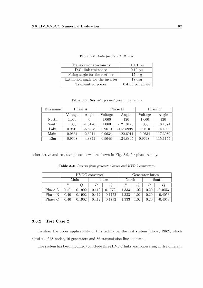
3.6. HVDC-LCC Numerical Evaluation 62
Table 3.2: Data for the HVDC link.
Transformer reactances 0.051 puD.C. link resistance 0.10 pu
Firing angle for the rectifier 15 degExtinction angle for the inverter 18 deg
Transmitted power 0.4 pu per phase
Table 3.3: Bus voltages and generation results.
Bus name Phase A Phase B Phase CVoltage Angle Voltage Angle Voltage Angle
North 1.060 0 1.060 -120 1.060 120South 1.000 -1.8126 1.000 -121.8126 1.000 118.1874Lake 0.9610 -5.5998 0.9610 -125.5998 0.9610 114.4002Main 0.9634 -2.6911 0.9634 -122.6911 0.9634 117.3089Elm 0.9648 -4.8845 0.9648 -124.8845 0.9648 115.1155
other active and reactive power flows are shown in Fig. 3.9, for phase A only.
Table 3.4: Powers from generator buses and HVDC converters.
HVDC converter Generator busesMain Lake North South
P Q P Q P Q P Q
Phase A 0.40 0.1902 0.412 0.1772 1.333 1.02 0.20 -0.4053Phase B 0.40 0.1902 0.412 0.1772 1.333 1.02 0.20 -0.4053Phase C 0.40 0.1902 0.412 0.1772 1.333 1.02 0.20 -0.4053
3.6.2 Test Case 2
To show the wider applicability of this technique, the test system [Chow, 1982], which
consists of 68 nodes, 16 generators and 86 transmission lines, is used.
The system has been modified to include three HVDC links, each operating with a different
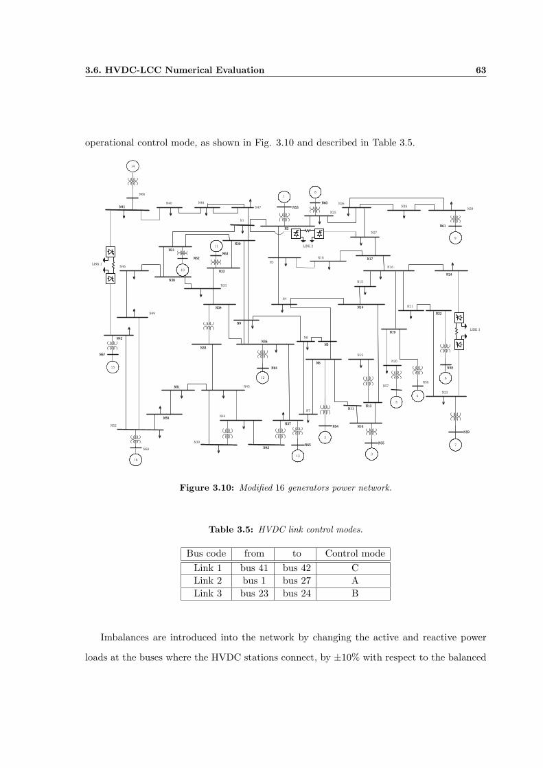
3.6. HVDC-LCC Numerical Evaluation 63
operational control mode, as shown in Fig. 3.10 and described in Table 3.5.
N41
N66
N2
N53
N60
N61
N17
N24
N14
N19
N22
N58
N59
N57
N5
N12
N6
N13N11
N10
N55
N54
N65
N37
N43
N64
N36
N9
N30
N32
N63
N34
N35
N51
N50
N42
N67
N38
N31
N62
14
10
9
8
1
13
16
15
12
2
6
11
4
5
7
3
N41
N48
N47
N1
N2
N53
N3
N60
N25
N26
N27
N28N29
N61
N17
N16
N24
N15
N14
N19
N21
N22
N58
N23
N59
N20
N56
N4
N5
N8
N6
N13N11
N10
N55
N54
N7
N65
N37
N43
N44
N39
N45
N64
N36
N9
N30
N32
N63
N33
N34
N35
N51
N50
N68
N52
N42
N67
N49
N38
N31
N62
N46
N40
N18
LINK 1
LINK 2
LINK 3
Figure 3.10: Modified 16 generators power network.
Table 3.5: HVDC link control modes.
Bus code from to Control modeLink 1 bus 41 bus 42 CLink 2 bus 1 bus 27 ALink 3 bus 23 bus 24 B
Imbalances are introduced into the network by changing the active and reactive power
loads at the buses where the HVDC stations connect, by ±10% with respect to the balanced
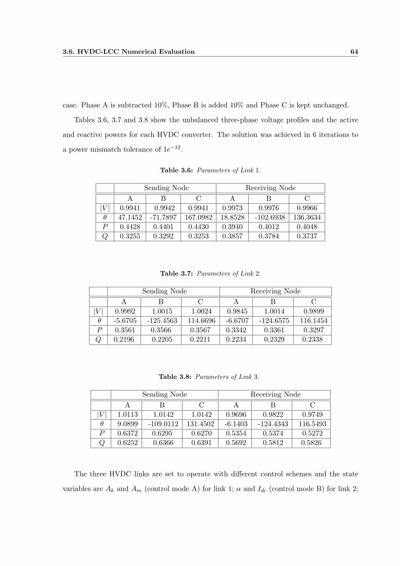
3.6. HVDC-LCC Numerical Evaluation 64
case. Phase A is subtracted 10%, Phase B is added 10% and Phase C is kept unchanged.
Tables 3.6, 3.7 and 3.8 show the unbalanced three-phase voltage profiles and the active
and reactive powers for each HVDC converter. The solution was achieved in 6 iterations to
a power mismatch tolerance of 1e−12.
Table 3.6: Parameters of Link 1.
Sending Node Receiving NodeA B C A B C
|V | 0.9941 0.9942 0.9941 0.9973 0.9976 0.9966θ 47.1452 -71.7897 167.0982 18.8528 -102.6938 136.3634P 0.4428 0.4401 0.4430 0.3940 0.4012 0.4048Q 0.3255 0.3292 0.3253 0.3857 0.3784 0.3737
Table 3.7: Parameters of Link 2.
Sending Node Receiving NodeA B C A B C
|V | 0.9992 1.0015 1.0024 0.9845 1.0014 0.9899θ -5.6705 -125.4563 114.6696 -6.6707 -124.6575 116.1454P 0.3561 0.3566 0.3567 0.3342 0.3361 0.3297Q 0.2196 0.2205 0.2211 0.2234 0.2329 0.2338
Table 3.8: Parameters of Link 3.
Sending Node Receiving NodeA B C A B C
|V | 1.0113 1.0142 1.0142 0.9696 0.9822 0.9749θ 9.0899 -109.0112 131.4502 -6.1403 -124.4343 116.5493P 0.6372 0.6295 0.6270 0.5354 0.5374 0.5272Q 0.6252 0.6366 0.6391 0.5692 0.5812 0.5826
The three HVDC links are set to operate with different control schemes and the state
variables are Ak and Am (control mode A) for link 1; α and Idc (control mode B) for link 2;
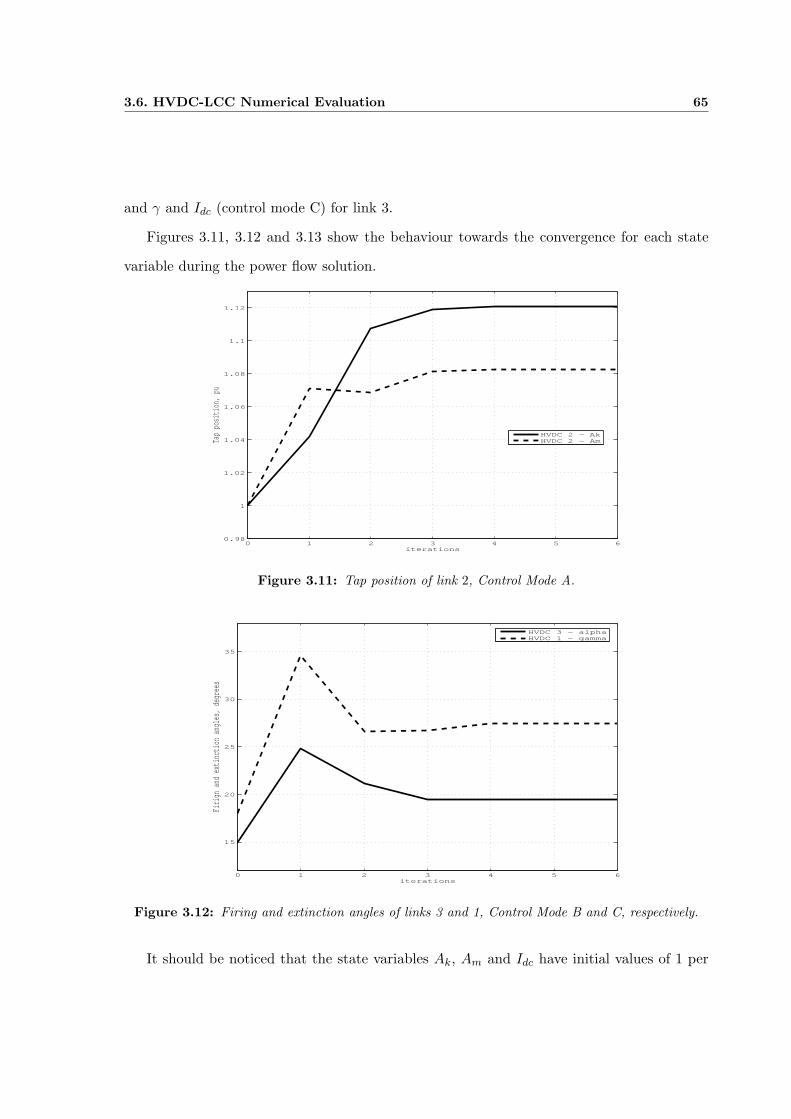
3.6. HVDC-LCC Numerical Evaluation 65
and γ and Idc (control mode C) for link 3.
Figures 3.11, 3.12 and 3.13 show the behaviour towards the convergence for each state
variable during the power flow solution.
0 1 2 3 4 5 60.98
1
1.02
1.04
1.06
1.08
1.1
1.12
iterations
Tap
posit
ion, p
u
HVDC 2 − AkHVDC 2 − Am
Figure 3.11: Tap position of link 2, Control Mode A.
0 1 2 3 4 5 6
15
20
25
30
35
iterations
Firign
and e
xtinc
tion a
ngles
, deg
rees
HVDC 3 − alphaHVDC 1 − gamma
Figure 3.12: Firing and extinction angles of links 3 and 1, Control Mode B and C, respectively.
It should be noticed that the state variables Ak, Am and Idc have initial values of 1 per
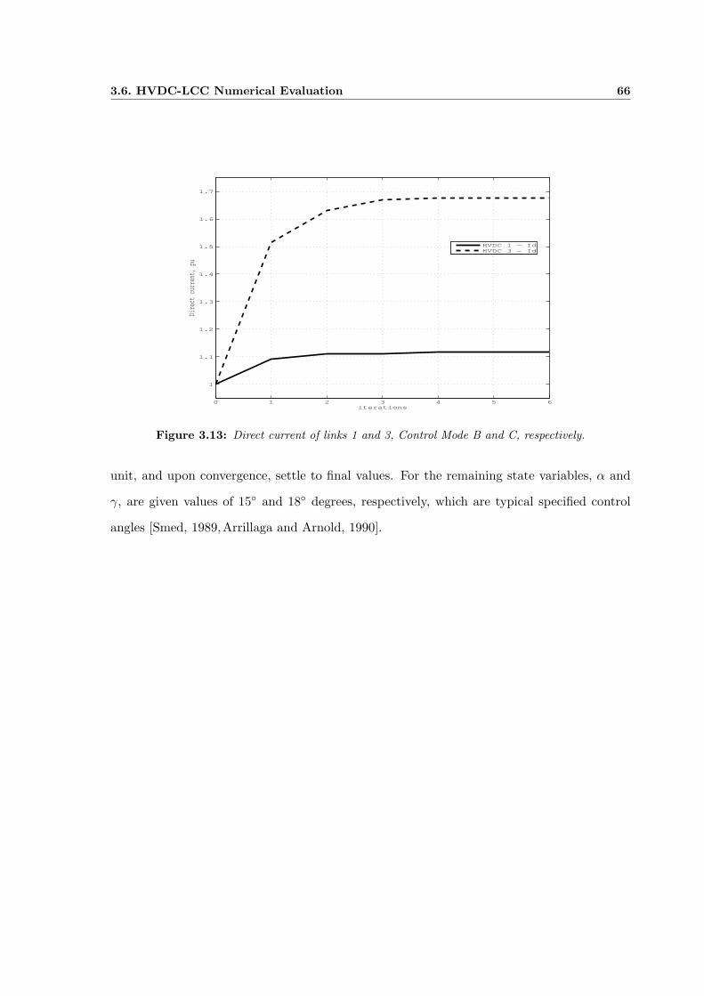
3.6. HVDC-LCC Numerical Evaluation 66
0 1 2 3 4 5 6
1
1.1
1.2
1.3
1.4
1.5
1.6
1.7
iterations
Dire
ct cu
rrent
, pu
HVDC 1 − IdHVDC 3 − Id
Figure 3.13: Direct current of links 1 and 3, Control Mode B and C, respectively.
unit, and upon convergence, settle to final values. For the remaining state variables, α and
γ, are given values of 15◦ and 18◦ degrees, respectively, which are typical specified control
angles [Smed, 1989,Arrillaga and Arnold, 1990].

3.7. Summary 67
3.7 Summary
This chapter presents the theory and modelling to carry out three-phase power flows
analyses in rectangular co-ordinates making use of the Newton-Raphson method.
The problem formulation, the Jacobian formation and its power equations, in three-phase
rectangular co-ordinates making use of the Newton-Raphson method is mentioned.
The adopted technique posses the quadratic convergence capability given by the Newton-
Raphson method. Despite of the number of equations to solve the load flow problem in
rectangular co-ordinates are increased in comparison with the polar algorithm, the problem
can be alleviated using sparsity techniques.
Moreover, this chapter presents a three-phase power flow method to include conventional
HVDC link models where several control modes are applied. The approach takes advantage
of the strong convergence characteristics of the Newton-Raphson technique to ensure reliable
iterative solutions. A test case is presented for a large network including unbalanced loading
and three HVDC links; each operating with its own control mode.
Chapter 4
Dynamic Power Flows in
Rectangular Co-ordinates
4.1 Introduction
Power flows in a power network can be assessed very affectively by modelling the power
system as a set of non-linear algebraic equations corresponding to active and reactive nodal
injections, valid for a pre-defined set of system generation and load.
For dynamic power system assessments, the mathematical model which described the
dynamic plant components such as generators and their controls are represented by a set of
differential equations.
By suitable combination of both sets of equations the complete power system model,
aimed to at time response calculations of large-scale power networks, can be reduced to an
algebraic-differential problem of the form,
y = F (y, x) (4.1)
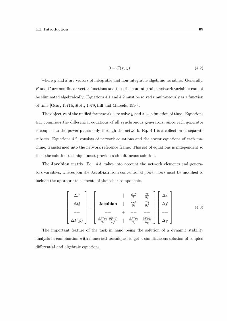
4.1. Introduction 69
0 = G(x, y) (4.2)
where y and x are vectors of integrable and non-integrable algebraic variables. Generally,
F and G are non-linear vector functions and thus the non-integrable network variables cannot
be eliminated algebraically. Equations 4.1 and 4.2 must be solved simultaneously as a function
of time [Gear, 1971b,Stott, 1979,Hill and Mareels, 1990].
The objective of the unified framework is to solve y and x as a function of time. Equations
4.1, comprises the differential equations of all synchronous generators, since each generator
is coupled to the power plants only through the network, Eq. 4.1 is a collection of separate
subsets. Equations 4.2, consists of network equations and the stator equations of each ma-
chine, transformed into the network reference frame. This set of equations is independent so
then the solution technique must provide a simultaneous solution.
The Jacobian matrix, Eq. 4.3, takes into account the network elements and genera-
tors variables, whereupon the Jacobian from conventional power flows must be modified to
include the appropriate elements of the other components.
∆P
∆Q
−−∆F (y)
=
| ∂P∂e
∂P∂f
Jacobian | ∂Q∂e
∂Q∂f
−− + −− −−∂F (y)
∂e∂F (y)
∂f | ∂F (y)∂y
∂F (y)∂y
∆e
∆f
−−∆y
(4.3)
The important feature of the task in hand being the solution of a dynamic stability
analysis in combination with numerical techniques to get a simultaneous solution of coupled
differential and algebraic equations.
4.2. Synchronous Machine Model - Classical Representation 70
4.2 Synchronous Machine Model - Classical Representation
Synchronous generators are the most important and principal sources of electric energy
at any power system. The power system stability problem is mainly related keeping to inter-
connected synchronous machines in synchronism. However, power system dynamic problems
are basically those of the synchronous machines. There are many kinds of power system dy-
namics problems, like high or low frequency oscillations, large or small system disturbances,
and so on. Owing to the wide range of dynamic phenomena, several synchronous machine
models have been put forward in the open literature.
The mechanical equations of synchronous machines are well established [Weedy, 1967,
Elgerd, 1971, Stevenson Jr, 1982,Chapman, 1991], so they are only briefly outlined. Three
basic assumptions are made in deriving the equations:
1. Machine rotor speed does not vary greatly from synchronous speed.
2. Machine rotational losses due to windage and friction are neglected.
3. Mechanical power shaft is smooth; it means the power which comes from the shaft is
constant except for the action of a speed governor.
From the previous assumptions, in particular from the second one, the power of the
machine Pa is the difference between the shaft power Pm as supplied by the prime mover and
the electrical power Pe. The acceleration is thus:
σ =Pa
Mg=
Pm − Pe
Mg(4.4)
where σ represents the acceleration of the machine, Mg is the angular momentum and
the powers are given in per unit.
It is convenient to choose a synchronously rotating reference to define the rotor angle δ.
Thus,
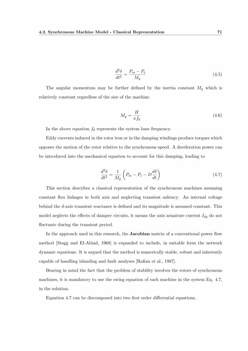
4.2. Synchronous Machine Model - Classical Representation 71
d2δ
dt2=
Pm − Pe
Mg(4.5)
The angular momentum may be further defined by the inertia constant Mg which is
relatively constant regardless of the size of the machine.
Mg =H
πf0(4.6)
In the above equation f0 represents the system base frequency.
Eddy currents induced in the rotor iron or in the damping windings produce torques which
opposes the motion of the rotor relative to the synchronous speed. A deceleration power can
be introduced into the mechanical equation to account for this damping, leading to
d2δ
dt2=
1Mg
(Pm − Pe −D
dδ
dt
)(4.7)
This section describes a classical representation of the synchronous machines assuming
constant flux linkages in both axis and neglecting transient saliency. An internal voltage
behind the d-axis transient reactance is defined and its magnitude is assumed constant. This
model neglects the effects of damper circuits, it means the axis armature current Idq do not
fluctuate during the transient period.
In the approach used in this research, the Jacobian matrix of a conventional power flow
method [Stagg and El-Abiad, 1968] is expanded to include, in suitable form the network
dynamic equations. It is argued that the method is numerically stable, robust and inherently
capable of handling islanding and fault analyses [Rafian et al., 1987].
Bearing in mind the fact that the problem of stability involves the rotors of synchronous
machines, it is mandatory to use the swing equation of each machine in the system Eq. 4.7,
in the solution.
Equation 4.7 can be discomposed into two first order differential equations,
4.2. Synchronous Machine Model - Classical Representation 72
ω =πf0
H[Pm − Pe −D (ω − ω0)] (4.8)
δ = ω − ω0 (4.9)
where
H is the inertia constant, MW*s/MVA.
Pm is the mechanical input power, pu.
Pe is the electrical output power, pu.
D is the damping coefficient, s/rad.
f0 is the synchronous frequency, Hz.
δ is the load angle, rad.
The classical derivation of the voltages and reactances which exists in a synchronous
machine are well established [Kimbark, 1948b, Concordia, 1951]. The electrical quantities
will be defined under the following assumptions:
1. All inductances are independent of the current.
2. Machine winding can be represented as constants.
3. Distributed windings may be represented as concentrated windings.
4. The machine is represented by a voltage behind the reactance.
5. There are no hysteresis losses in the iron.
6. The leakage reactance occurs only in the stator.
Using these assumptions the classical model for a synchronous machine is constructed.
With reference to Fig. 4.1, assuming balanced conditions, the algebraic equations that
describe generator voltage relations can be written by a set of equations based on direct and
quadrature axis parameters,
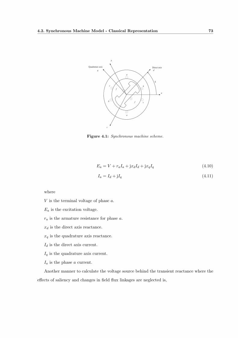
4.2. Synchronous Machine Model - Classical Representation 73
Quadrature axis
q
Direct axis
d
b
a
c
f
f
a
a
b
bc
c
d
Figure 4.1: Synchronous machine scheme.
Ea = V + raIa + jxdId + jxqIq (4.10)
Ia = Id + jIq (4.11)
where
V is the terminal voltage of phase a.
Ea is the excitation voltage.
ra is the armature resistance for phase a.
xd is the direct axis reactance.
xq is the quadrature axis reactance.
Id is the direct axis current.
Iq is the quadrature axis current.
Ia is the phase a current.
Another manner to calculate the voltage source behind the transient reactance where the
effects of saliency and changes in field flux linkages are neglected is,
4.3. Synchronous Machines Controllers 74
Ea = |E| (cos δE + j sin δE) (4.12)
4.3 Synchronous Machines Controllers
Power-generating plants consist of various components involved in energy conversion from
mechanical to electrical. The main elements involved in most dynamic voltage stability
analyses are the generators, voltage regulators, governors, turbines, boilers, and auxiliary
equipment.
This section illustrates suitable models for voltage stability assessment.
4.3.1 Governor
The governor is a frequency controller which plays an important role in power system
operations. It has three main functions which are:
1. To keep the generator speed as close as possible to its nominal value.
2. To guarantee a fast and automatic participation of the generator to any change in
generation, which is required in order to maintain a balanced generation-load in the
system.
3. To offer a way to adapt the active power production of the unit, via speed-changer
adjustments.
The governor adjusts the steam or water input to the turbine. To achieve this, it senses the
difference between the actual rotor speed and the angular frequency and adjusts accordingly
the turbine valve.
Figure 4.2 shows the block diagram adopted to represent the speed governing system for
steam generators. This is the simplified model proposed in [IEEE Committee Report, 1973].
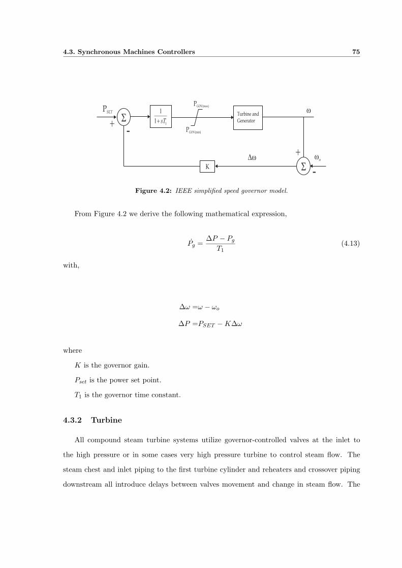
4.3. Synchronous Machines Controllers 75
STurbine andGenerator
PGOV(max)
PGOV(min)
wPSET
+
-1
1
1 sT+
SK
Dw wo
+
-
Figure 4.2: IEEE simplified speed governor model.
From Figure 4.2 we derive the following mathematical expression,
Pg =∆P − Pg
T1(4.13)
with,
∆ω =ω − ωo
∆P =PSET −K∆ω
where
K is the governor gain.
Pset is the power set point.
T1 is the governor time constant.
4.3.2 Turbine
All compound steam turbine systems utilize governor-controlled valves at the inlet to
the high pressure or in some cases very high pressure turbine to control steam flow. The
steam chest and inlet piping to the first turbine cylinder and reheaters and crossover piping
downstream all introduce delays between valves movement and change in steam flow. The
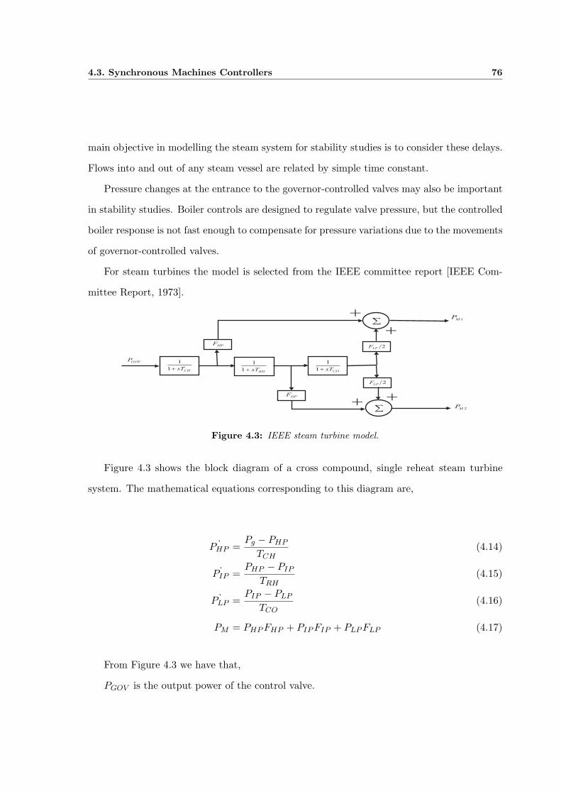
4.3. Synchronous Machines Controllers 76
main objective in modelling the steam system for stability studies is to consider these delays.
Flows into and out of any steam vessel are related by simple time constant.
Pressure changes at the entrance to the governor-controlled valves may also be important
in stability studies. Boiler controls are designed to regulate valve pressure, but the controlled
boiler response is not fast enough to compensate for pressure variations due to the movements
of governor-controlled valves.
For steam turbines the model is selected from the IEEE committee report [IEEE Com-
mittee Report, 1973].
å
GOVP
+
CHsT+1
1
HPF
RHsT+1
1
å
COsT+1
1
2LP
F
2LP
F
+
+
HPF
+
1MP
2MP
Figure 4.3: IEEE steam turbine model.
Figure 4.3 shows the block diagram of a cross compound, single reheat steam turbine
system. The mathematical equations corresponding to this diagram are,
˙PHP =Pg − PHP
TCH(4.14)
˙PIP =PHP − PIP
TRH(4.15)
˙PLP =PIP − PLP
TCO(4.16)
PM = PHP FHP + PIP FIP + PLP FLP (4.17)
From Figure 4.3 we have that,
PGOV is the output power of the control valve.
4.3. Synchronous Machines Controllers 77
TCH is the steam chest time constant (including the high-pressure (HP ) stage of the
turbine time constant).
TRH is the reheater time constant (including the intermediate-pressure (IP ) stage of the
turbine time constant).
TCO is the steam storage or cross-over time constant (including the low-pressure (LP )
stage of the turbine time constant).
FHP is the HP turbine power fraction.
FIP is the IP turbine power fraction.
FLP is the LP turbine power fraction.
PM1 and PM2 are the equivalent generator input mechanical powers.
4.3.3 Automatic voltage regulator
The basic function of an AVR is to provide direct current to the field winding of a
synchronous machine. In addition, the excitation system can provide a broad number of
control and protection functions necessary for the satisfactory performance of the machine
and the power system by means of the control of the field voltage. The protective functions
ensure that the capacity limits of both synchronous machine and excitation control system
will not be exceeded.
Several Automatic Voltage Regulator (AVR) models have been developed for transient
stability studies. The model adopted in this simulation tool, is the STA1 IEEE model [Energy
Development and Power Generating Committe of the PES, 2003, IEEE Committee Report,
1981].
The main objective of an AVR is to provide an effective control of the generator terminal
voltage and, hence, the enhancement of system stability.
From Figure 4.4, the following expressions are derived:

4.3. Synchronous Machines Controllers 78
Vr(max)
Vr(min)
+
-1
a
a
K
sT++
-Vref
1
1r
sT+
V
-
-
1
f
f
K s
sT+
1
1e
sT+
EVr
Se
Figure 4.4: STA1 IEEE AVR model.
˙Vm =V − Vm
Tr(4.18)
˙Vr1 =Ka
(Vref − Vm − Vr2 − Kf
TfVf
)− Vr1
Ta(4.19)
˙Vr2 =−Kf
TfVf + Vr2
Tf(4.20)
Vf =− (Vf (1 + Se(Vf ))− Vr)Te
(4.21)
where the ceiling function Se is defined as:
Se(Vf ) = Ae
(eBe|Vf | − 1
)(4.22)
where,
Vr max is the maximum regulator voltage, pu.
Vr min is the minimum regulator voltage, pu.
Ka is the amplifier gain, pu.
Ta is the amplifier time constant, sec.
Kf is the stabiliser gain, pu.
Tf is the stabiliser time constant, sec.

4.4. Synchronous Machine Model - Advanced Representation 79
Te is the field circuit time constant, sec.
Tr is the measurement time constant, sec.
Ae is the 1st ceiling coefficient.
Be is the 2nd ceiling coefficient.
4.3.4 Boiler
The boiler model presented here is a simple model which takes into account the slow plant
response. The equations that formulate the boiler storage, throttle pressure, and the change
in the flow of the steam into the steam chest according to the boiler response are:
∆DP =SF −∆PHP
CB(4.23)
∆PHP = PHP − (Pset − k3∆ω) (4.24)
˙PHP =Pg + k1∆DP − PHP
TCH(4.25)
where,
DP is the throttle pressure.
SF is the steam production.
k3 is the gain factor to regulate the effect of frequency deviation on boiler response.
Equation 4.25 will replace Eq. B.12 to allow the effects of pressure change in the boiler
an the steam flow into the turbine.
4.4 Synchronous Machine Model - Advanced Representation
In early stability studies calculations the generators were commonly represented by a
simple model, assuming constant flux linkages in each axis and neglecting transient saliency
[Stagg and El-Abiad, 1968]. In these simple models an internal voltage behind the d-axis

4.4. Synchronous Machine Model - Advanced Representation 80
transient reactance xd is determined and its magnitude is assumed constant.
Due to the inertia of the flux linkages, faster changes in the conditions external to the
synchronous machine are presented, and these changes are not reflected throughout the whole
of the model immediately.
In order to get a more realistic representation of the power system behaviour, it is essential
to consider transient saliency and the flux linkages in each axis of the synchronous machine.
Figure 4.5 depicts the phasor diagram of synchronous machine in the transient state.
Direct axis
Quadrature axis
Ei
E’q
E’d
E’
Eq
Ed
Ef
IqX
q
IdX
d
IdX’
d
IqX’
q
IRa
V
I
Iq
Id
Figure 4.5: Phasor diagram of synchronous generator in the transient state.
Thus, the voltage behind synchronous reactance Ea, should be obtained with the voltages,
E′d and E′
q. To obtain these voltages, it is necessary to obtain the voltages which will represent
the flux linkages of the rotor windings.
The differential equations that describe the variation in time of the rotor flux linkages
are:
E′q =
Ea + (xd − x′d) Id −E′q
T ′do
(4.26)
E′d =
−E′d −
(xq − x′q
)Iq
T ′qo
(4.27)
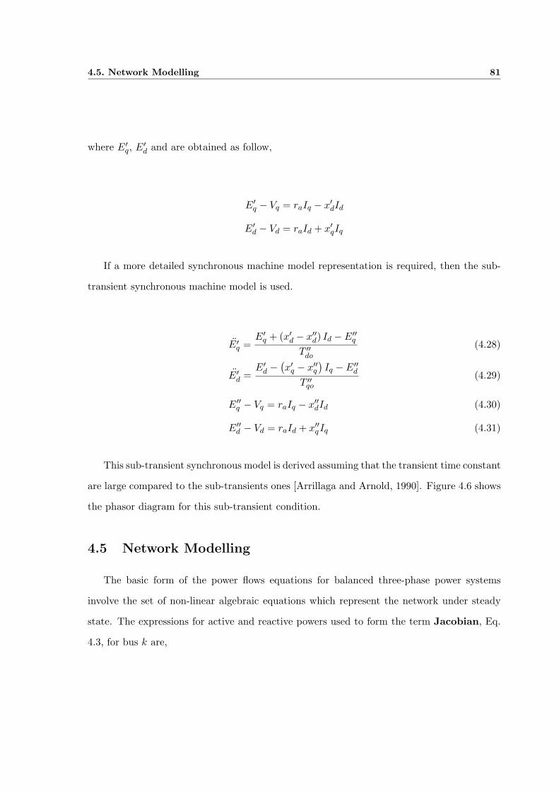
4.5. Network Modelling 81
where E′q, E′
d and are obtained as follow,
E′q − Vq = raIq − x′dId
E′d − Vd = raId + x′qIq
If a more detailed synchronous machine model representation is required, then the sub-
transient synchronous machine model is used.
E′q =
E′q + (x′d − x′′d) Id −E′′
q
T ′′do
(4.28)
E′d =
E′d −
(x′q − x′′q
)Iq − E′′
d
T ′′qo
(4.29)
E′′q − Vq = raIq − x′′dId (4.30)
E′′d − Vd = raId + x′′qIq (4.31)
This sub-transient synchronous model is derived assuming that the transient time constant
are large compared to the sub-transients ones [Arrillaga and Arnold, 1990]. Figure 4.6 shows
the phasor diagram for this sub-transient condition.
4.5 Network Modelling
The basic form of the power flows equations for balanced three-phase power systems
involve the set of non-linear algebraic equations which represent the network under steady
state. The expressions for active and reactive powers used to form the term Jacobian, Eq.
4.3, for bus k are,
4.6. Transmission Line Model 82
Direct axis
Quadrature axis
Ei
E’’q
E’’d
E’’
Eq
Ed
Ef
IqX
q
IdX
d
IdX’’
d
IqX’’
q
IRa
V
I
Iq
Id
E’
Figure 4.6: Phasor diagram of synchronous generator in the sub-transient state.
Pk =ek
∑
m=1,n
(Gkmem −Bkmfm) + fk
∑
m=1,n
(Gkmfm + Bkmem) (4.32)
Qk =fk
∑
m=1,n
(Gkmem −Bkmfm)− ek
∑
m=1,n
(Gkmfm + Bkmem) (4.33)
where Pk and Qk are the active and reactive powers injected at bus k, ek and fk are the
voltage’s real and imaginary parts at bus k, Gkm and Bkm are the real and imaginary parts
of the nodal admittance relating buses k and m. It should be noted that k = m corresponds
to the self admittance of bus k. As shown below, each plant component of the power network
is represented by its own form of nodal admittance elements Gkk, Bkk, Gkm and Bkm.
4.6 Transmission Line Model
In power system studies it is common to represent a transmission line by its nominal π
circuit, shown in Fig. 4.7.
corresponding to a transmission line l of series impedance Zl and shunt admittance Yl. The
transmission line is connected between buses k and m, giving rise to the following transfer
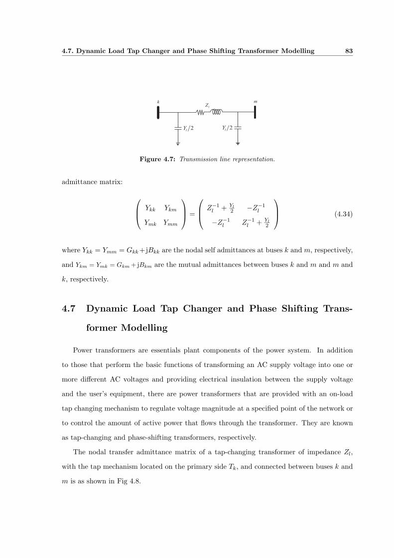
4.7. Dynamic Load Tap Changer and Phase Shifting Transformer Modelling 83
2l
Y
lZ
k m
2l
Y
Figure 4.7: Transmission line representation.
admittance matrix:
Ykk Ykm
Ymk Ymm
=
Z−1l + Yl
2 −Z−1l
−Z−1l Z−1
l + Yl2
(4.34)
where Ykk = Ymm = Gkk +jBkk are the nodal self admittances at buses k and m, respectively,
and Ykm = Ymk = Gkm + jBkm are the mutual admittances between buses k and m and m and
k, respectively.
4.7 Dynamic Load Tap Changer and Phase Shifting Trans-
former Modelling
Power transformers are essentials plant components of the power system. In addition
to those that perform the basic functions of transforming an AC supply voltage into one or
more different AC voltages and providing electrical insulation between the supply voltage
and the user’s equipment, there are power transformers that are provided with an on-load
tap changing mechanism to regulate voltage magnitude at a specified point of the network or
to control the amount of active power that flows through the transformer. They are known
as tap-changing and phase-shifting transformers, respectively.
The nodal transfer admittance matrix of a tap-changing transformer of impedance Zl,
with the tap mechanism located on the primary side Tk, and connected between buses k and
m is as shown in Fig 4.8.
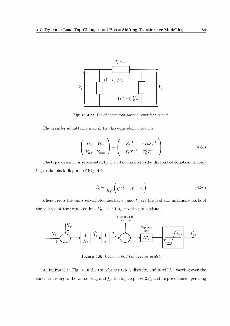
4.7. Dynamic Load Tap Changer and Phase Shifting Transformer Modelling 84
k lT Z
( )2
k k lT T Z-
( )1k l
T Z-
kV
mV
Figure 4.8: Tap-changer transformer equivalent circuit.
The transfer admittance matrix for this equivalent circuit is:
Ykk Ykm
Ymk Ymm
=
Z−1l −TkZ
−1l
−TkZ−1l T 2
k Z−1l
(4.35)
The tap’s dynamic is represented by the following first-order differential equation, accord-
ing to the block diagram of Fig. 4.9.
Tk =1
HT
(√e2k + f2
k − V0
)(4.36)
where HT is the tap’s servomotor inertia, ek and fk are the real and imaginary parts of
the voltage at the regulated bus, V0 is the target voltage magnitude.
V0
+
-1
TH
1
s
Vk
n
-
+
kT
kTD
Tap step
size
maxkT
kT& 1k
T
minkT
Current Tap
position
Figure 4.9: Dynamic load tap changer model.
As indicated in Fig. 4.10 the transformer tap is discrete, and it will be varying over the
time, according to the values of ek and fk, the tap step size ∆Tk and its pre-defined operating

4.8. Numerical Solution Technique 85
range.
kV low
V
highV
posT
0
2
3
4
1
Figure 4.10: Discrete tap.
The nodal transfer admittance matrix of a phase-changing transformer of impedance Zl,
with the phase angle mechanism located on the primary side φk, and connected between
buses k and m, is:
Ykk Ykm
Ymk Ymm
=
Z−1l −Z−1
l (cosφk + j sinφk)
−Z−1l (cosφk − j sinφk) T 2
k Z−1l
(4.37)
The tap’s dynamic is represented by the following first order differential equation:
φk =1
Hφ(Pkm − P0) (4.38)
where Hφ is the phase shifter’s servomotor inertia, Pkm is the active power through the phase
shifter, P0 is the target active power.
4.8 Numerical Solution Technique
The set of algebraic and differential equations that describe each plant component of the
power network are interdependent and it has been suggested that their simultaneous calcu-
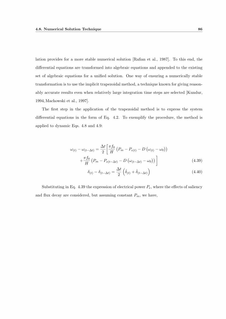
4.8. Numerical Solution Technique 86
lation provides for a more stable numerical solution [Rafian et al., 1987]. To this end, the
differential equations are transformed into algebraic equations and appended to the existing
set of algebraic equations for a unified solution. One way of ensuring a numerically stable
transformation is to use the implicit trapezoidal method, a technique known for giving reason-
ably accurate results even when relatively large integration time steps are selected [Kundur,
1994,Machowski et al., 1997].
The first step in the application of the trapezoidal method is to express the system
differential equations in the form of Eq. 4.2. To exemplify the procedure, the method is
applied to dynamic Eqs. 4.8 and 4.9:
ω(t) − ω(t−∆t) =∆t
2
[πf0
H
(Pm − Pe(t) −D
(ω(t) − ω0
))
+πf0
H
(Pm − Pe(t−∆t) −D
(ω(t−∆t) − ω0
)) ](4.39)
δ(t) − δ(t−∆t) =∆t
2
(δ(t) + δ(t−∆t)
)(4.40)
Substituting in Eq. 4.39 the expression of electrical power Pe, where the effects of saliency
and flux decay are considered, but assuming constant Pm, we have,
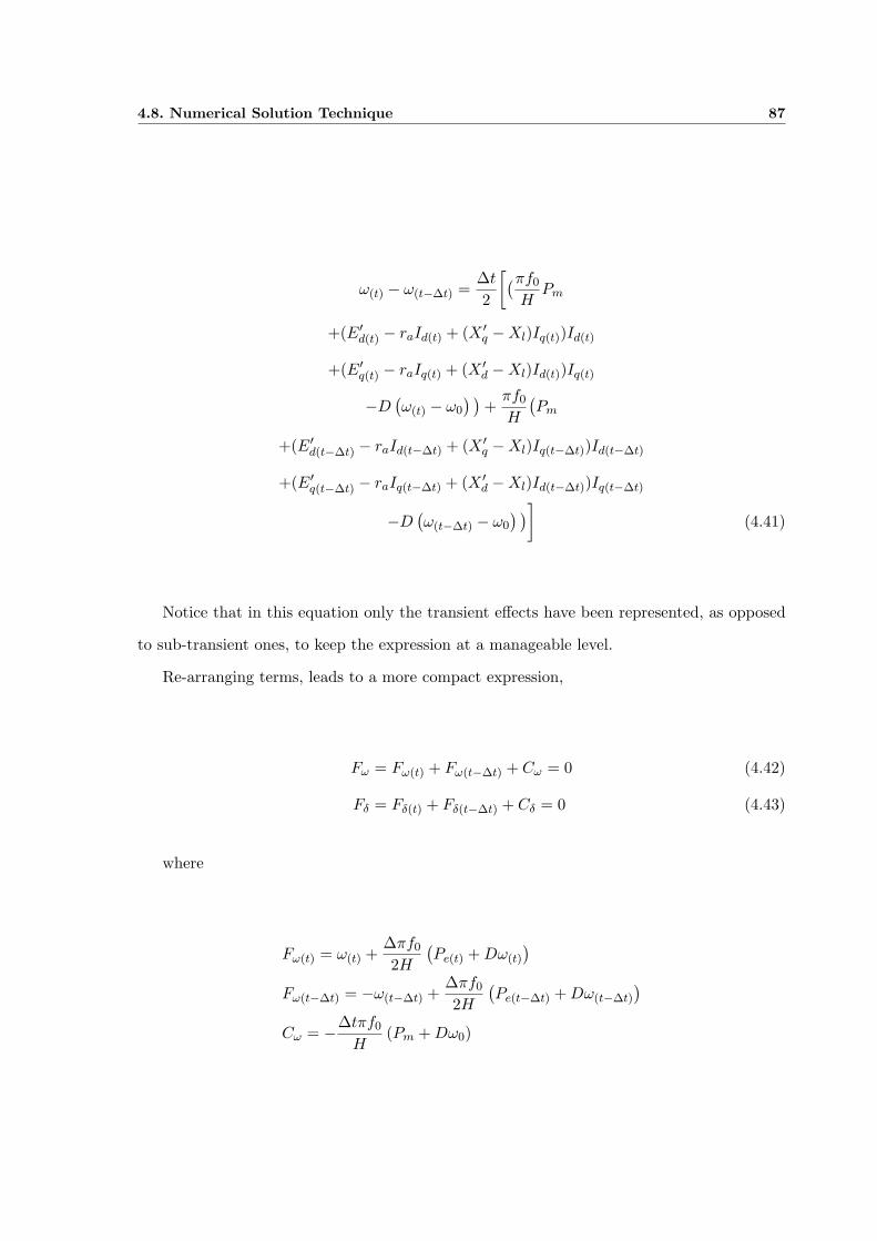
4.8. Numerical Solution Technique 87
ω(t) − ω(t−∆t) =∆t
2
[(πf0
HPm
+(E′d(t) − raId(t) + (X ′
q −Xl)Iq(t))Id(t)
+(E′q(t) − raIq(t) + (X ′
d −Xl)Id(t))Iq(t)
−D(ω(t) − ω0
) )+
πf0
H
(Pm
+(E′d(t−∆t) − raId(t−∆t) + (X ′
q −Xl)Iq(t−∆t))Id(t−∆t)
+(E′q(t−∆t) − raIq(t−∆t) + (X ′
d −Xl)Id(t−∆t))Iq(t−∆t)
−D(ω(t−∆t) − ω0
) )](4.41)
Notice that in this equation only the transient effects have been represented, as opposed
to sub-transient ones, to keep the expression at a manageable level.
Re-arranging terms, leads to a more compact expression,
Fω = Fω(t) + Fω(t−∆t) + Cω = 0 (4.42)
Fδ = Fδ(t) + Fδ(t−∆t) + Cδ = 0 (4.43)
where
Fω(t) = ω(t) +∆πf0
2H
(Pe(t) + Dω(t)
)
Fω(t−∆t) = −ω(t−∆t) +∆πf0
2H
(Pe(t−∆t) + Dω(t−∆t)
)
Cω = −∆tπf0
H(Pm + Dω0)
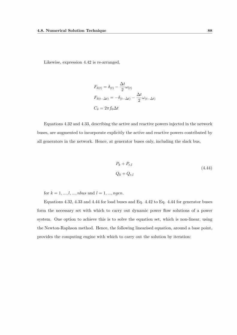
4.8. Numerical Solution Technique 88
Likewise, expression 4.42 is re-arranged,
Fδ(t) = δ(t) −∆t
2ω(t)
Fδ(t−∆t) = −δ(t−∆t) −∆t
2ω(t−∆t)
Cδ = 2πf0∆t
Equations 4.32 and 4.33, describing the active and reactive powers injected in the network
buses, are augmented to incorporate explicitly the active and reactive powers contributed by
all generators in the network. Hence, at generator buses only, including the slack bus,
Pk + Pe,l
Qk + Qe,l
(4.44)
for k = 1, ..., l, ..., nbus and l = 1, ..., ngen.
Equations 4.32, 4.33 and 4.44 for load buses and Eq. 4.42 to Eq. 4.44 for generator buses
form the necessary set with which to carry out dynamic power flow solutions of a power
system. One option to achieve this is to solve the equation set, which is non-linear, using
the Newton-Raphson method. Hence, the following linearised equation, around a base point,
provides the computing engine with which to carry out the solution by iteration:
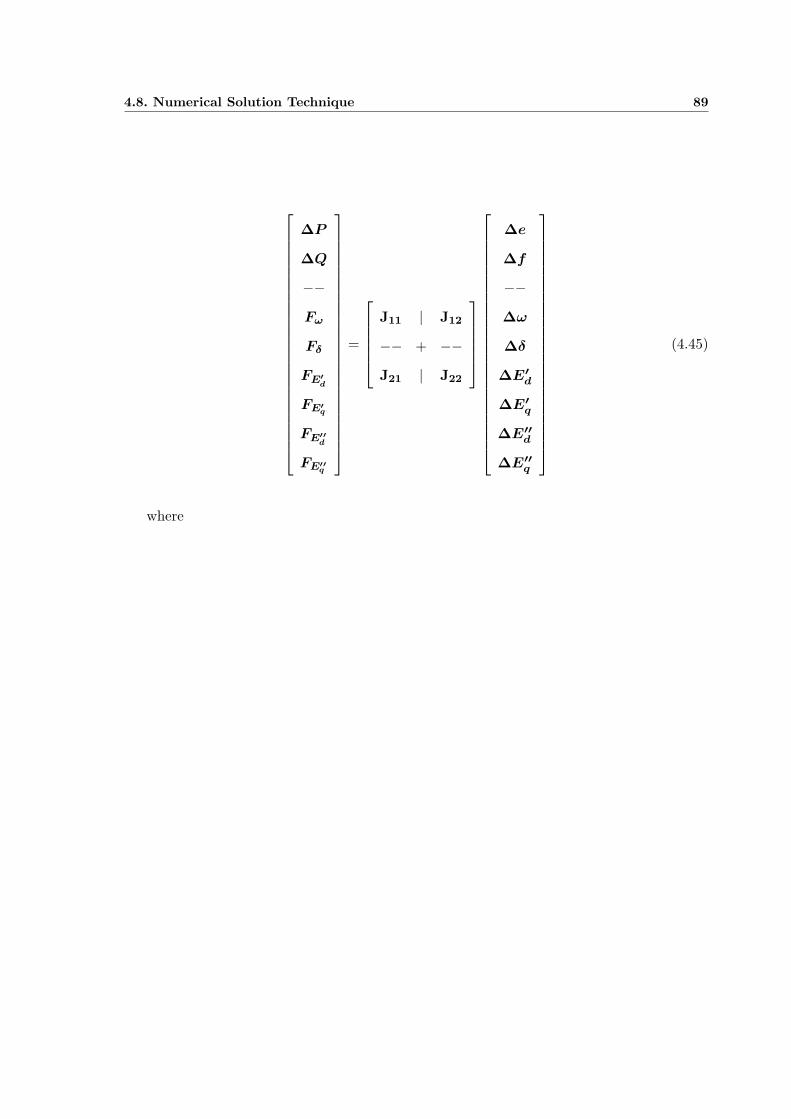
4.8. Numerical Solution Technique 89
∆P
∆Q
−−Fω
Fδ
FE′d
FE′q
FE′′d
FE′′q
=
J11 | J12
−− + −−J21 | J22
∆e
∆f
−−∆ω
∆δ
∆E′d
∆E′q
∆E′′d
∆E′′q
(4.45)
where

4.8. Numerical Solution Technique 90
∆P = [∆P1, . . . ,∆Pn]t
∆Q = [∆Q1, . . . ,∆Qn]t
∆e = [∆e1, . . . , ∆en]t
∆f = [∆f1, . . . , ∆fn]t
∆ω = [∆ω1, . . . , ∆ωm]t
∆δ = [∆δ1, . . . ,∆ + δm]t
∆E′d =
[∆E′
d1, . . . , ∆E′
dm
]t
∆E′q =
[∆E′
q1, . . . ,∆E′
qm
]t
∆E′′d =
[∆E′′
d1, . . . , ∆E′
dm
]t
∆E′′q =
[∆E′′
q1, . . . ,∆E′
qm
]t
Fω = [Fω1 , . . . , Fωm ]t
Fδ = [Fδ1 , . . . , Fδm ]t
FE′d=
[FE′d1
, . . . , FE′dm
]t
FE′q =[FE′q1
, . . . , FE′qm
]t
FE′′d=
[FE′′d1
, . . . , FE′′dm
]t
FE′′q =[FE′′q1
, . . . , FE′′qm
]t
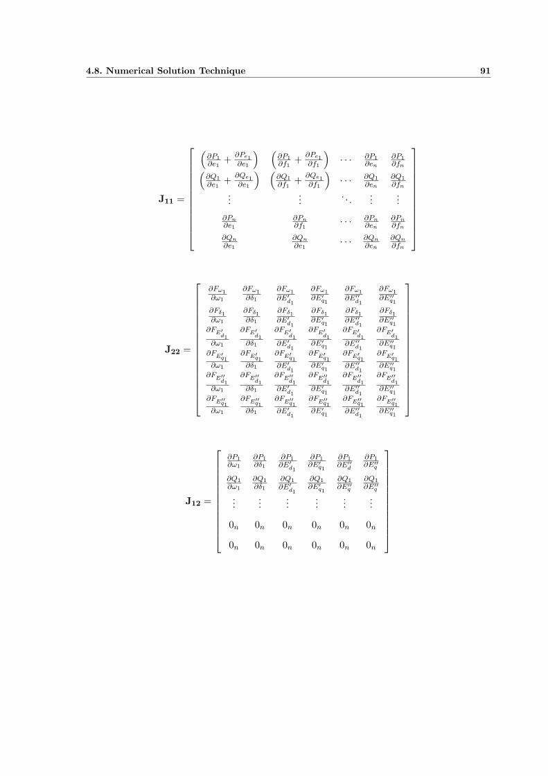
4.8. Numerical Solution Technique 91
J11 =
(∂P1∂e1
+ ∂Pe1∂e1
) (∂P1∂f1
+ ∂Pe1∂f1
)· · · ∂P1
∂en
∂P1∂fn(
∂Q1
∂e1+ ∂Qe1
∂e1
) (∂Q1
∂f1+ ∂Qe1
∂f1
)· · · ∂Q1
∂en
∂Q1
∂fn
......
. . ....
...
∂Pn∂e1
∂Pn∂f1
· · · ∂Pn∂en
∂Pn∂fn
∂Qn
∂e1
∂Qn
∂e1· · · ∂Qn
∂en
∂Qn
∂fn
J22 =
∂Fω1∂ω1
∂Fω1∂δ1
∂Fω1∂E′d1
∂Fω1∂E′q1
∂Fω1∂E′′d1
∂Fω1∂E′′q1
∂Fδ1∂ω1
∂Fδ1∂δ1
∂Fδ1∂E′d1
∂Fδ1∂E′q1
∂Fδ1∂E′′d1
∂Fδ1∂E′′q1
∂FE′d1
∂ω1
∂FE′d1
∂δ1
∂FE′d1
∂E′d1
∂FE′d1
∂E′q1
∂FE′d1
∂E′′d1
∂FE′d1
∂E′′q1∂FE′q1∂ω1
∂FE′q1∂δ1
∂FE′q1∂E′d1
∂FE′q1∂E′q1
∂FE′q1∂E′′d1
∂FE′q1∂E′′q1
∂FE′′d1
∂ω1
∂FE′′d1
∂δ1
∂FE′′d1
∂E′d1
∂FE′′d1
∂E′q1
∂FE′′d1
∂E′′d1
∂FE′′d1
∂E′′q1∂FE′′q1∂ω1
∂FE′′q1∂δ1
∂FE′′q1∂E′d1
∂FE′′q1∂E′q1
∂FE′′q1∂E′′d1
∂FE′′q1∂E′′q1
J12 =
∂P1∂ω1
∂P1∂δ1
∂P1∂E′d1
∂P1∂E′q1
∂P1∂E′′d
∂P1∂E′′q
∂Q1
∂ω1
∂Q1
∂δ1∂Q1
∂E′d1
∂Q1
∂E′q1∂Q1
∂E′′q∂Q1
∂E′′q...
......
......
...
0n 0n 0n 0n 0n 0n
0n 0n 0n 0n 0n 0n

4.8. Numerical Solution Technique 92
J21 =
∂Fω1∂e1
∂Fω1∂f1
· · · 0n 0n
∂Fδ1∂e1
∂Fδ1∂f1
· · · 0n 0n
∂FE′d1
∂e1
∂FE′d1
∂f1· · · 0n 0n
∂FE′d1
∂e1
∂FE′d1
∂f1· · · 0n 0n
∂FE′′d1
∂e1
∂FE′′d1
∂f1· · · 0n 0n
∂FE′′q1∂e1
∂FE′′q1∂f1
· · · 0n 0n
J11 is a matrix of first order partial derivatives of the active and reactive power, P and
Q, with respect to nodal voltages, e,f . The active and reactive powers contributed by the
generators are taken into consideration in the Jacobian term, J11. J22 is a matrix of partial
derivatives of generators discretised functions of the form of Eq. 4.42 and Eq. 4.43, with
respect to generator state variables ω, δ, E′d, E′
q, E′′d and E′′
q . J12 is a matrix of first order
partial derivatives of active and reactive power at generator buses with respect to generator
state variables. J21 is a matrix of first order partial derivatives of generator discretised
functions of the form of Eq. 4.42 and Eq. 4.43, with respect to nodal voltages e,f .
Equation 4.45 may be seen as an extended Newton-Raphson power flow formulation in
rectangular coordinates, where the generating plant equations, in discretised form, are lin-
earised and solved together with the normal power flow equations, including those of the
slack bus generator. In the overall Jacobian, in addition to the entries corresponding to the
generating plant itself there are mutual terms corresponding to the interface between the
network and the generating plant.
It should be remarked that in Eq. 4.45 the mechanical power Pm contributed by the
boiler-turbine-governor set has been taken to remain constant, for the sake of simplifying
the equation. In practice, however, the boiler-turbine-governor set is an important dynamic
element in power systems long term dynamics and the linearised Eq. 4.45 should be suitably
expanded to accommodate an expression of the form:
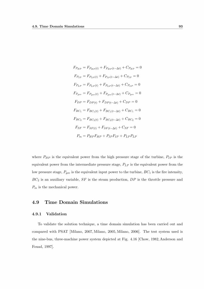
4.9. Time Domain Simulations 93
FPHP= FPHP (t) + FPHP (t−∆t) + CPHP
= 0
FPIP= FPIP (t) + FPIP (t−∆t) + CPIP
= 0
FPLP= FPLP (t) + FPLP (t−∆t) + CPLP
= 0
FPgov = FPgov(t) + FPgov(t−∆t) + CPgov = 0
FDP = FDP (t) + FDP (t−∆t) + CDP = 0
FBC1 = FBC1(t) + FBC1(t−∆t) + CBC1 = 0
FBC2 = FBC2(t) + FBC2(t−∆t) + CBC2 = 0
FSF = FSF (t) + FSF (t−∆t) + CSF = 0
Pm = PHP FHP + PIP FIP + PLP PLP
where PHP is the equivalent power from the high pressure stage of the turbine, PIP is the
equivalent power from the intermediate pressure stage, PLP is the equivalent power from the
low pressure stage, Pgov is the equivalent input power to the turbine, BC1 is the fire intensity,
BC2 is an auxiliary variable, SF is the steam production, DP is the throttle pressure and
Pm is the mechanical power.
4.9 Time Domain Simulations
4.9.1 Validation
To validate the solution technique, a time domain simulation has been carried out and
compared with PSAT [Milano, 2007, Milano, 2005, Milano, 2006]. The test system used is
the nine-bus, three-machine power system depicted at Fig. 4.16 [Chow, 1982,Anderson and
Fouad, 1997].
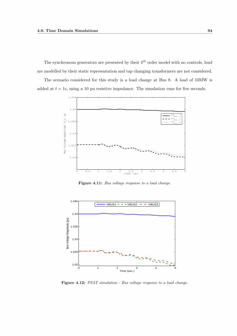
4.9. Time Domain Simulations 94
The synchronous generators are presented by their 4th order model with no controls, load
are modelled by their static representation and tap changing transformers are not considered.
The scenario considered for this study is a load change at Bus 8. A load of 10MW is
added at t = 1s, using a 10 pu resistive impedance. The simulation runs for five seconds.
0 0.5 1 1.5 2 2.5 3 3.5 4 4.5 5
1.02
1.025
1.03
1.035
1.04
1.045
time, sec
Bus
volt
age
magn
itud
e |V
i|,
pu |VBus 1
|
|VBus 2
|
|VBus 3
|
Figure 4.11: Bus voltage response to a load change.
0 1 2 3 4 51.02
1.025
1.03
1.035
1.04
1.045
Time (sec.)
Bus
Volta
ge M
agni
tude
(pu)
VBUS1 VBUS2 VBUS3
Figure 4.12: PSAT simulation - Bus voltage response to a load change.

4.9. Time Domain Simulations 95
It should be noted from Fig. 4.11 and Fig. 4.12, that the system response at Bus 1, is
more damped than those at Buses 2 and 3. This is due to the fact that former buses are
closer to the perturbation point.
0 0.5 1 1.5 2 2.5 3 3.5 4 4.5 50.6
0.8
1
1.2
1.4
1.6
1.8
time, sec
Elec
tric
al p
ower
Pe, p
u
Gen1
Gen2
Gen3
Figure 4.13: Electrical power deliver by generators.
Fig. 4.13 shows the electrical power delivered by the generators during the transient
simulation. Fig. 4.14 presents the machines angle differences. It is noted that the angular
differences of the machines are small, thus, the system will remain stable after the disturbance.
Fig. 4.15 shows the speed deviation for the synchronous generators.
4.9.2 A classical stability study
Even when the simultaneous solution technique adopted is particularly suited to carrying
out long-term assessments of voltage stability in power systems, it can also handle transient
stability analyses. So then, the solution technique is illustrated by solving the classical
transient stability study depicted at [Anderson and Fouad, 1997].
The nine-bus system [Chow, 1982,Anderson and Fouad, 1997], shown at Fig. 4.16, is used
to conduct this analyses.
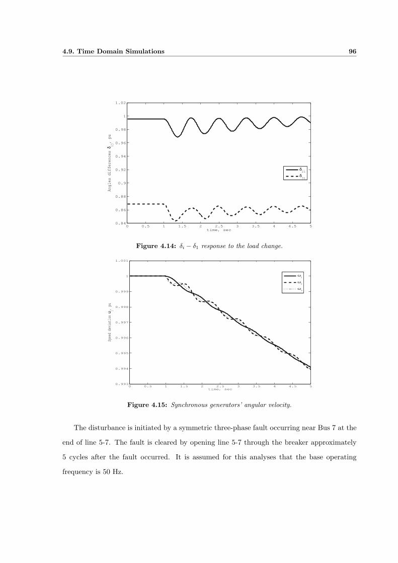
4.9. Time Domain Simulations 96
0 0.5 1 1.5 2 2.5 3 3.5 4 4.5 50.84
0.86
0.88
0.9
0.92
0.94
0.96
0.98
1
1.02
time, sec
Angles differences δ
ij, pu
δ21
δ31
Figure 4.14: δi − δ1 response to the load change.
0 0.5 1 1.5 2 2.5 3 3.5 4 4.5 50.993
0.994
0.995
0.996
0.997
0.998
0.999
1
1.001
time, sec
Speed deviation
ω i, pu
ω1
ω2
ω3
Figure 4.15: Synchronous generators’ angular velocity.
The disturbance is initiated by a symmetric three-phase fault occurring near Bus 7 at the
end of line 5-7. The fault is cleared by opening line 5-7 through the breaker approximately
5 cycles after the fault occurred. It is assumed for this analyses that the base operating
frequency is 50 Hz.

4.9. Time Domain Simulations 97
Bus 1
Bus 2 Bus 3
Bus 4
Bus 5 Bus 6
Bus 7
Bus 8
Bus 9
Gen. 2 Gen. 3
Gen. 1
TRANF1
TRANF2 TRANF3
Figure 4.16: 3 Generators 9 buses power system.
For this stability assessment, synchronous generator are modelled by their classical rep-
resentation with no controls.
The variables plotted are the generator’s speed, ωi, generator’s rotor angle, δi, and the
buses voltage magnitude, |Vi|.Figures 4.17-4.21 show the result for this dynamic assessment, with Fig. 4.17 showing
the voltage magnitude at the system buses. In Fig. 4.18 the response of the machine’s
rotor angle, δi, is presented. Fig. 4.19 gives the angle differences between machines, namely,
δ21 = δ2− δ1 and δ31 = δ3− δ1. This plot indicates that the system remains stable. This fact
is clearly indicated by the angular differences of the machines which are not divergent even
though their response is oscillatory.
Figure 4.20 shows the speed deviation for the synchronous generators, and Fig. 4.21
shows the voltage magnitude for the buses where the synchronous generators are connected
to.
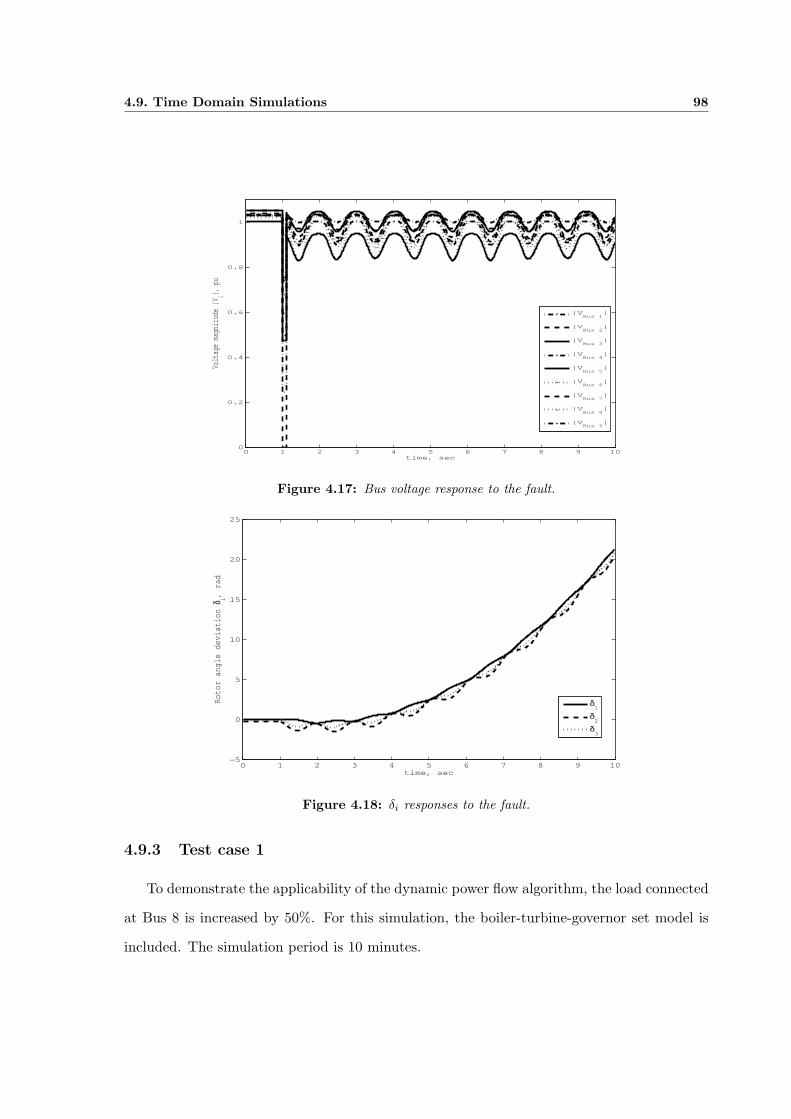
4.9. Time Domain Simulations 98
0 1 2 3 4 5 6 7 8 9 100
0.2
0.4
0.6
0.8
1
time, sec
Volt
age
magn
itud
e |V
i|,
pu
|VBus 1
|
|VBus 2
|
|VBus 3
|
|VBus 4
|
|VBus 5
|
|VBus 6
|
|VBus 7
|
|VBus 8
|
|VBus 9
|
Figure 4.17: Bus voltage response to the fault.
0 1 2 3 4 5 6 7 8 9 10−5
0
5
10
15
20
25
time, sec
Rot
or a
ngle
dev
iatio
n δ i, r
ad
δ1
δ2
δ3
Figure 4.18: δi responses to the fault.
4.9.3 Test case 1
To demonstrate the applicability of the dynamic power flow algorithm, the load connected
at Bus 8 is increased by 50%. For this simulation, the boiler-turbine-governor set model is
included. The simulation period is 10 minutes.
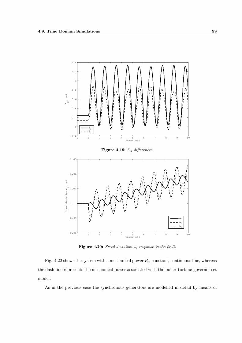
4.9. Time Domain Simulations 99
0 1 2 3 4 5 6 7 8 9 10−0.2
0
0.2
0.4
0.6
0.8
1
1.2
1.4
time, sec
δ ij, r
ad
δ21
δ31
Figure 4.19: δij differences.
0 1 2 3 4 5 6 7 8 9 100.98
0.99
1
1.01
1.02
1.03
time, sec
Spee
d de
viat
ion
ω i,
rad
ω1
ω2
ω3
Figure 4.20: Speed deviation ωi response to the fault.
Fig. 4.22 shows the system with a mechanical power Pm constant, continuous line, whereas
the dash line represents the mechanical power associated with the boiler-turbine-governor set
model.
As in the previous case the synchronous generators are modelled in detail by means of

4.9. Time Domain Simulations 100
0 1 2 3 4 5 6 7 8 9 10
0.5
0.6
0.7
0.8
0.9
1
1.1
time, sec
Volt
age
magn
itud
e |V
i|,
pu
|VBus 1
|
|VBus 2
|
|VBus 3
|
Figure 4.21: Voltage magnitude for generator buses.
0 2 4 6 8 100.6
0.8
1
1.2
1.4
1.6
1.8
time, min
Mechanical power P
m, pu
Figure 4.22: Synchronous generators’ mechanical power.
the subtransient model. Fig 4.23 shows the excitation voltage |Ef | for the case when the
boiler-turbine-governor set is considered. Fig 4.24 depicts the voltage magnitudes for the
systems’ buses.
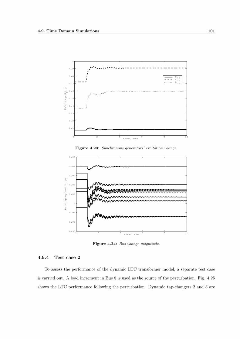
4.9. Time Domain Simulations 101
0 2 4 6 8 101
1.1
1.2
1.3
1.4
1.5
1.6
1.7
1.8
1.9
2
time, min
Field volatge |E
f|, pu
|Ef 1
|
|Ef 2
|
|Ef 3
|
Figure 4.23: Synchronous generators’ excitation voltage.
0 2 4 6 8 100.97
0.98
0.99
1
1.01
1.02
1.03
1.04
1.05
time, min
Bus voltage magnitude |V
i|, pu
Figure 4.24: Bus voltage magnitude.
4.9.4 Test case 2
To assess the performance of the dynamic LTC transformer model, a separate test case
is carried out. A load increment in Bus 8 is used as the source of the perturbation. Fig. 4.25
shows the LTC performance following the perturbation. Dynamic tap-changers 2 and 3 are
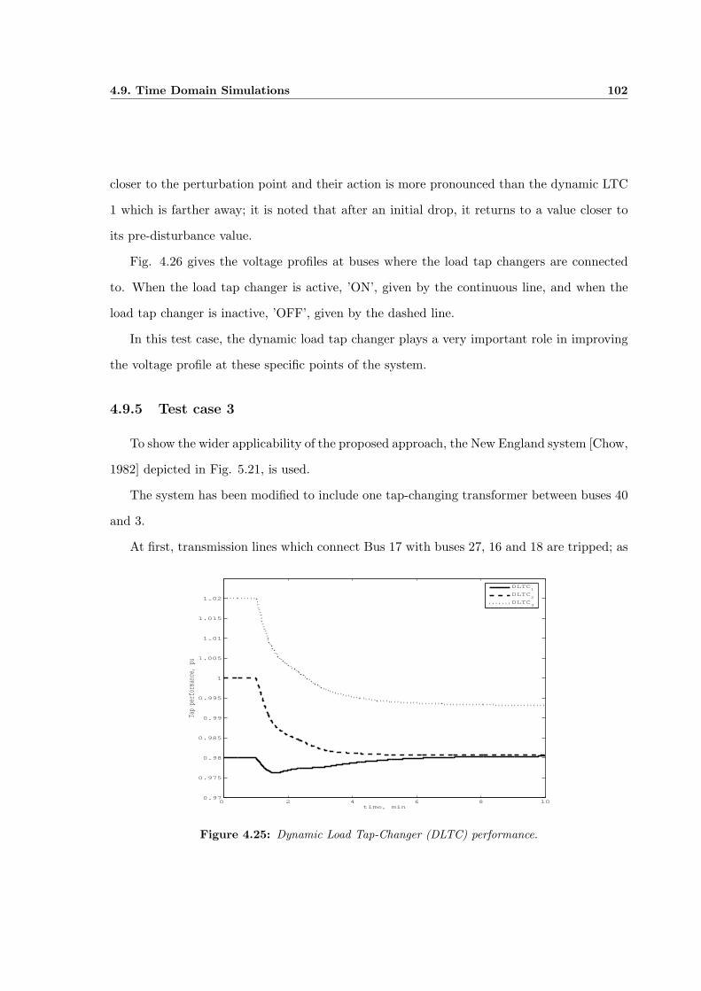
4.9. Time Domain Simulations 102
closer to the perturbation point and their action is more pronounced than the dynamic LTC
1 which is farther away; it is noted that after an initial drop, it returns to a value closer to
its pre-disturbance value.
Fig. 4.26 gives the voltage profiles at buses where the load tap changers are connected
to. When the load tap changer is active, ’ON’, given by the continuous line, and when the
load tap changer is inactive, ’OFF’, given by the dashed line.
In this test case, the dynamic load tap changer plays a very important role in improving
the voltage profile at these specific points of the system.
4.9.5 Test case 3
To show the wider applicability of the proposed approach, the New England system [Chow,
1982] depicted in Fig. 5.21, is used.
The system has been modified to include one tap-changing transformer between buses 40
and 3.
At first, transmission lines which connect Bus 17 with buses 27, 16 and 18 are tripped; as
0 2 4 6 8 100.97
0.975
0.98
0.985
0.99
0.995
1
1.005
1.01
1.015
1.02
time, min
Tap
perf
orma
nce,
pu
DLTC1
DLTC2
DLTC3
Figure 4.25: Dynamic Load Tap-Changer (DLTC) performance.

4.9. Time Domain Simulations 103
0 5 10 15 20 251
1.01
1.02
1.03
1.04
1.05
time, min
|VBus 4|
0 5 10 15 20 250.98
1
1.02
1.04
time, min
|VBus 7|
0 5 10 15 20 250.99
1
1.01
1.02
1.03
1.04
time, min
|VBus 9|
Figure 4.26: Voltage magnitude at Buses 4, 7 and 9.
a consequence Bus 17 including its load, is isolated from the system, producing a voltage drop
at the majority of nodes. Next, the transmission line connecting buses 3 and 18 is taken out
of service, causing that node 18 and its load become separated from the system, bringing a
recovery of system voltages. This is followed by a tripping of the transmission line connecting
buses 3 to 4; an event that triggers a voltage collapse of the entire system.
Fig. 4.28 shows the voltage magnitudes in the remaining 37 buses of the system. Fig.
4.29 shows the discrete response of the tap-changer under abrupt voltage changes. It can be
seen that this device works in its pre-specified working range, which is from 0.90 to 1.10. The
tap changer performance can be observed in Fig. 4.29.
Fig. 4.30 shows the voltage profile at the bus where the voltage is controlled by the
tap-changer. As shown, the tap-changer transformer is able to control the voltage around its
specified value, 1 p.u., even when the system is undergoing unfavourable conditions.
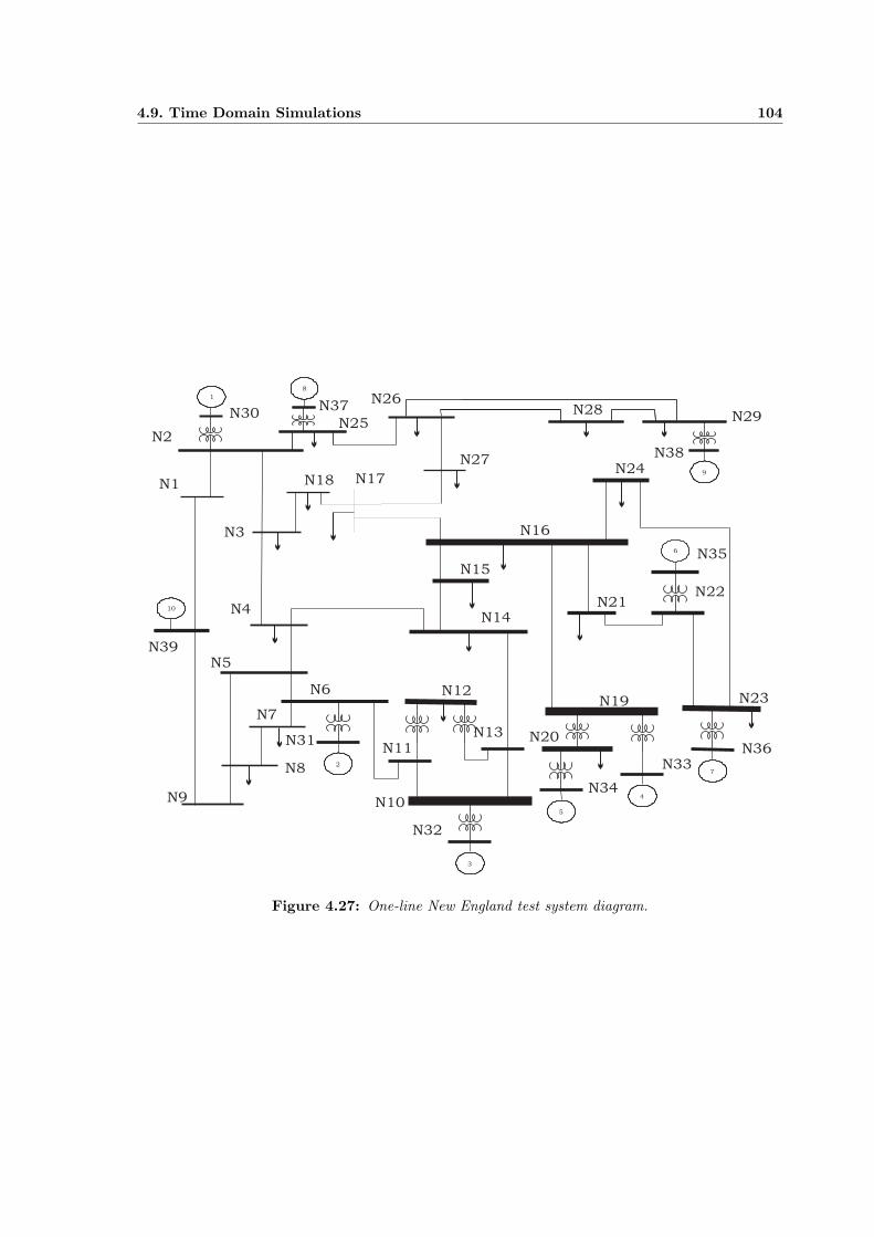
4.9. Time Domain Simulations 104
N30N37
N38
9
8
10
N2
N25
N26N28
N29
1
2
3
5
4
7
N1 N18 N17
N27
N3
N39
N4
N5
N6
N7
N8
N9
N31
N12
N11
N10
N13
N32
N34
N20
N19
N33
N36
N23
N21N22
N356
N15
N16
N24
N14
Figure 4.27: One-line New England test system diagram.
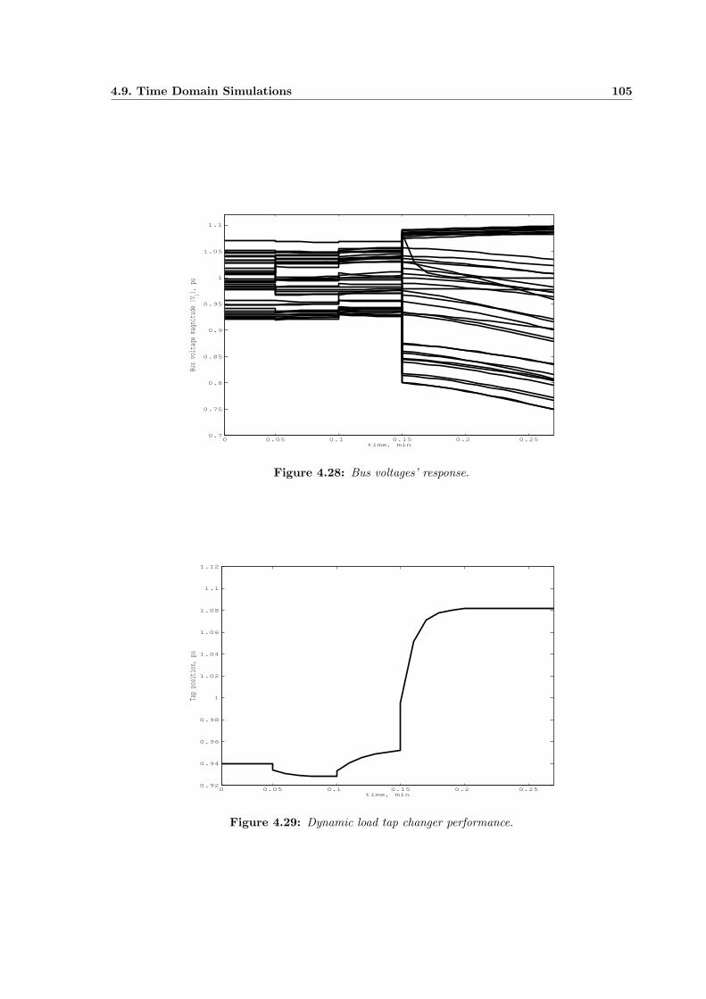
4.9. Time Domain Simulations 105
0 0.05 0.1 0.15 0.2 0.250.7
0.75
0.8
0.85
0.9
0.95
1
1.05
1.1
time, min
Bus
volt
age
magn
itud
e |V
i|,
pu
Figure 4.28: Bus voltages’ response.
0 0.05 0.1 0.15 0.2 0.250.92
0.94
0.96
0.98
1
1.02
1.04
1.06
1.08
1.1
1.12
time, min
Tap position, pu
Figure 4.29: Dynamic load tap changer performance.
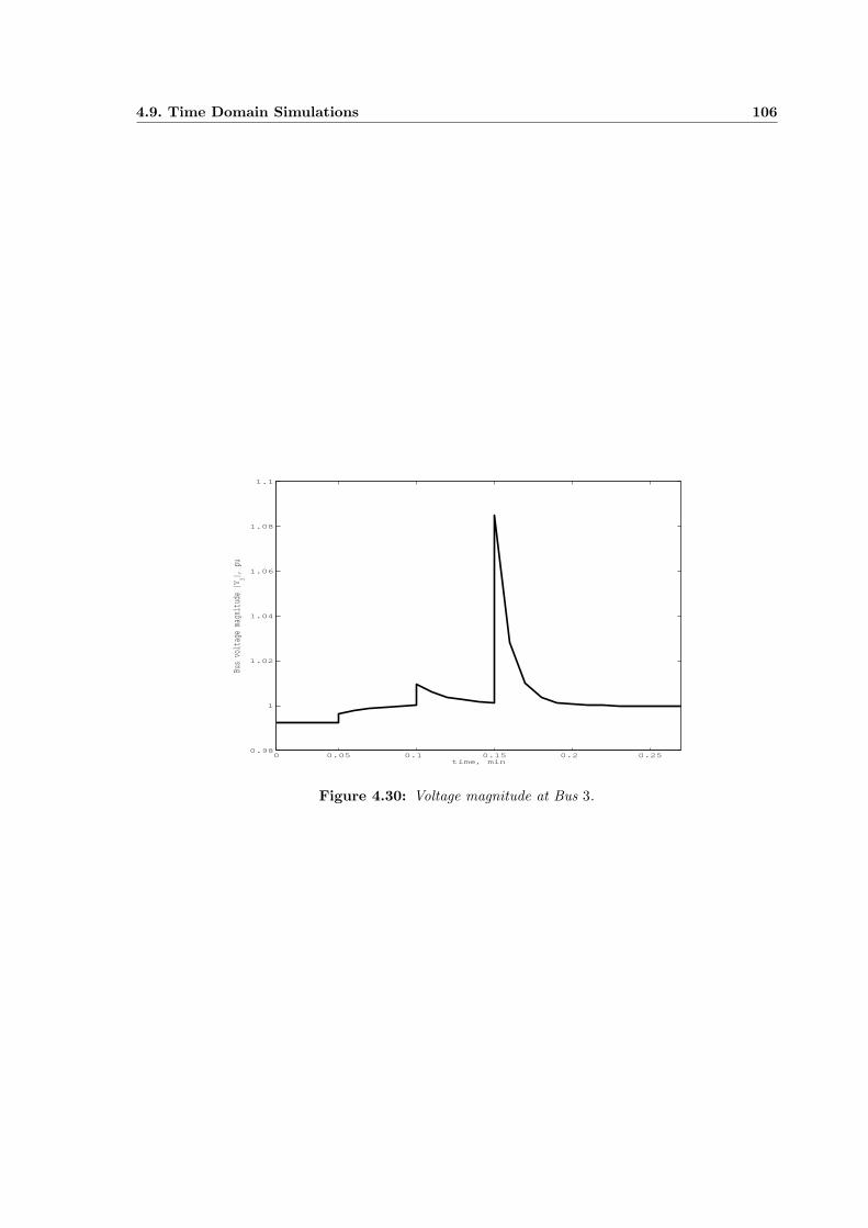
4.9. Time Domain Simulations 106
0 0.05 0.1 0.15 0.2 0.250.98
1
1.02
1.04
1.06
1.08
1.1
time, min
Bus voltage magnitude |V
3|, pu
Figure 4.30: Voltage magnitude at Bus 3.
4.10. Summary 107
4.10 Summary
This chapter focuses on the dynamic model of generating plants. For the purpose of this
research, dynamic stability assessment, mathematical models of the classical synchronous
machine model and the advanced representation of it, with automatic voltage regulator,
turbine, speed-governor and boiler, in a balanced three-phase frame of reference have been
developed. A set of ordinary differential equations describing the components was obtained for
each generating plant component. In each case, the differential equations of each component
are transformed into an algebraic form taking advantage of the implicit trapezoidal rule.
The differential-algebraic model of the network has been coded in software to carry out time
domain analyses of power networks with combined dynamic and static elements. An implicit
trapezoidal integration method embedded with a Newton-Raphson iteration technique has
been selected to solve simultaneously, the differential and static system equations. The models
and the solution method have been proven capable of performing adequately the long-term
dynamic assessment of power systems. The trapezoidal rule is applied to discretise the
dynamic equations corresponding to all the synchronous generators’ variables and power
plant components.
Several network disturbances, such as tripping lines, load variations and balanced three-
phase faults have been studied using the developed algorithm. Where appropriate, the results
reported are compared with the output of PSAT [Milano, 2007,Milano, 2005,Milano, 2006], a
widely used transient stability simulation package within the academic community, yielding
satisfactory agreement.
Chapter 5
Power System Loads Modelling
5.1 Load Modelling Concepts
5.1.1 Introduction
Over the past several years, the increasing concern over voltage stability has lead to an
enormous effort in industry to develop acceptable techniques and tools for analysis of this
phenomena [Taylor, 1994,IEEE Power Engineering Society, 2002,Morison et al., 1993]. Since
voltage stability is characteristically different from other forms of stability, such as transient
stability or small signal stability, new analytical and modeling approaches were required.
Both steady-state (static) analyses methods (such as PV curves and modal analyses) and
dynamic analyses (such as time-domain simulation) have gained industry acceptance and are
now widely used.
An important step in the development of analyses methods involves identifying and de-
veloping models for system components, devices, and controls which are key to the voltage
stability phenomenon. These include such examples as the modelling of reactive capability of
generators including over-excitation limiters, Static Var Systems, automatic under-load tap-
changer transformers, automatically switched capacitors, and load-shedding schemes. In gen-
5.1. Load Modelling Concepts 109
eral, these can be considered deterministic modelling issues; the device structures/functions
are not explicitly time-varying and once known, can be modelled with a reasonable degree
of certainty. However, the driving force for voltage instability is usually the loads, which
can be considered highly statistical in nature and, therefore, much more of a challenge when
developing practical models which are generically applicable. Studies have shown that the
results of stability simulations can be drastically affected by variations in load models; this is
particularly true for voltage stability studies in which loads may be subjected to large varia-
tions in system voltages and in which short-term and long-term non-linear load characteristics
may come into play. While there has been significant attention given to load modelling in
industry [IEEE Load Task Force, 1993, IEEE Task Force on Load Representation, 1995,Xu
and Mansour, 1994,Hagajos and Danai, 1998], including numerous IEEE and CIGRE pub-
lications, for most engineers, it remains a challenge to properly develop load models which
can be used with confidence in practical day-to-day studies.
Power system engineers base decisions concerning system performance in large part on the
results of power flow and stability simulation studies. In performing power system analyses,
models must be developed for all relevant system components, including generating station,
transmission and distribution equipment and load devices.
Much attention has been given to models for generation and transmission/distribution
equipment as described in Chapter 4, and load representation has received a lack of attention
and continues to be an area of greater uncertainty.
Many studies have shown that load representation can have a significant impact on anal-
yses result [IEEE Load Task Force, 1993, IEEE Task Force on Load Representation, 1995].
Therefore, load modelling is of major importance and should be address and considered for
dynamic performance analyses.
For purposes of system studies, the term ”load” refers to the equivalent representation
of the aggregate effects of many individual load devices and the interconnecting distribution
and subtransmission systems that are not explicitly represented in the system model [IEEE
5.1. Load Modelling Concepts 110
Power Engineering Society, 2002].
Load characteristics affect the dynamic behaviour of a power system and the importance
of proper representation of loads in power system stability studies has long been recognized
[Concordia and Ihara, 1982].
Load modelling for dynamic performance analyses has been greatly advanced in the past
few years. A bibliographical review [IEEE Task Force on Load Representation, 1995] pub-
lished in 1995 contained 118 references on the subject. However, the representation of loads
for voltage stability analyses involves several aspects not required for conventional stabil-
ity studies. The modelling of these effects is not well-established and is still the subject of
ongoing investigation [IEEE Power Engineering Society, 2002].
For stability studies load representation is very common to be denoted by a load bus
which represents incandescent and fluorescent lamps, heaters, air conditioner, ovens, refrig-
erators, motors, arc furnaces and so on. Induction motors constitute a major portion of
the system load. The precise representation of load is difficult to estimate. Even when the
precise representation of load is known, there are many other factors like time (hour, day,
season), weather conditions and the state of the economy that prevent the load modelling in
power systems [Kundur, 1994]. Hence, load representation in stability studies is based on a
considerable amount of simplifications. The active and reactive power consumed by the load
could be represented by a simple mathematical model, and the load models can be divided
into two main categories:
a Static load model,
b Dynamic load model.
5.2. Static Load Model 111
5.2 Static Load Model
In transient stability studies simulations, loads are typically modelled as purely static,
(algebraic) functions according to their time responses to voltage and frequency variations in
the system.
The load model can be defined as a mathematical representation of the relation between
the active or reactive power (or the current injection) in a load bus and the complex voltage
of this same bus.
Regularly, static models were used in earlier attempts to model load elements. However,
to simplify the mathematical load expression frequency was considered constant, leading it
to a load expression where only the voltage dependency is considered.
5.2.1 Polynomial representation
Typically both active and reactive power loads are represented by quadratic polynomials
given by
P = P0
[a0
( |V ||V0|
)2
+ a1
( |V ||V0|
)+ a2
](5.1)
Q = Q0
[b0
( |V ||V0|
)2
+ b1
( |V ||V0|
)+ b2
](5.2)
where V0, P0 and Q0 are normally taken as initial operating conditions.
Fig. 5.1 shows this load model representation.
The load elements were divided into:
i Constant impedance ”Z”,
ii Constant current ”I” and
iii Constant power ”P”.
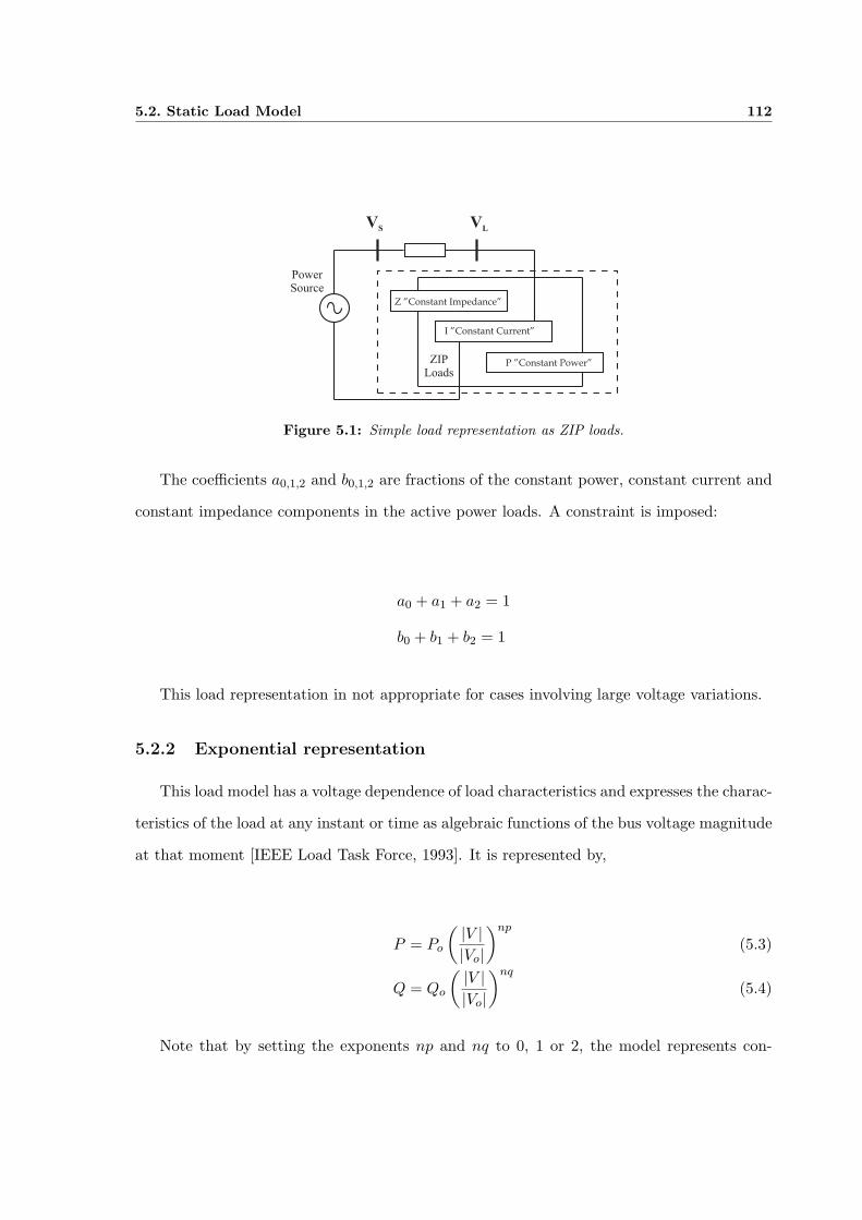
5.2. Static Load Model 112
VS
VL
Z ”Constant Impedance”
I ”Constant Current”
P ”Constant Power”ZIP
Loads
Power
Source
Figure 5.1: Simple load representation as ZIP loads.
The coefficients a0,1,2 and b0,1,2 are fractions of the constant power, constant current and
constant impedance components in the active power loads. A constraint is imposed:
a0 + a1 + a2 = 1
b0 + b1 + b2 = 1
This load representation in not appropriate for cases involving large voltage variations.
5.2.2 Exponential representation
This load model has a voltage dependence of load characteristics and expresses the charac-
teristics of the load at any instant or time as algebraic functions of the bus voltage magnitude
at that moment [IEEE Load Task Force, 1993]. It is represented by,
P = Po
( |V ||Vo|
)np
(5.3)
Q = Qo
( |V ||Vo|
)nq
(5.4)
Note that by setting the exponents np and nq to 0, 1 or 2, the model represents con-
5.3. Frequency Load Model 113
stant power, constant current or constant impedance characteristics, respectively. Exponents
greater than 2 or less than 0 may be appropriate for some types of loads [IEEE Load Task
Force, 1993].
For constant power model, the voltage is invariant and allows loads to be represented
with a stiff voltage characteristic. The constant current model gives a load demand that
varies linearly with voltage np ≈ nq ≈ 1. This is a practical representation of the real power
demand as a mixture of resistance and motor devices. Finally, for constant impedance model,
the load power changes proportionally np ≈ nq ≈ 2. This model represents lighting loads
but it does not model stiff loads satisfactorily.
5.3 Frequency Load Model
For this load modelling, a static load model representation may includes frequency de-
pendance. This is usually represented by expressing either a polynomial or exponential load
model multiplied by a factor of the following form,
(1 + apf∆f)
where ∆f is the frequency deviation, given by,
(f − f0)
where f is the frequency of the bus voltage, f0 is the rated frequency.
The value of apf normally ranges from 0 to 3.0 for the active contribution and from −2.0
to 0 for the reactive power contribution [Concordia and Ihara, 1982].
Usually, the bus voltage frequency is not an inherent state variable of the system however,
it can be computed by taking the numerical derivative of the bus voltage angle.

5.4. Dynamic Load Model 114
5.4 Dynamic Load Model
Despite the effort to get more accurate load models where the voltage/frequency depen-
dance is present [Hill, 1993, Anrborg et al., 1998], these models do not take into account
the dynamic of the load and are still being modelled as static loads. Thus, to modelled
the dynamic load behaviour in more detail where the voltage/frequency parameters and the
dynamic itself of any electrical power system could be represented, an induction motor load
representation is more than necessary.
In today’s power systems, the motors consume a large fraction of the electricity generated.
Hence, accurate modelling of these motors is required to capture the dynamics associated with
the motors.
There is wide-ranging agreement that load characteristics have a marked influence on
system stability, in general, and that induction motor loads play a dominate role during the
initial stages of a voltage instability occurrence [Sekine and Ohtsuki, 1990, Hill, 1993], in
particular.
5.4.1 Induction motor modelling
A simple and yet realistic model of the induction motor is used in the dynamic power
flows algorithm. It is based on the equivalent circuit shown in Fig. 5.2, and corresponds to
a single cage induction motor.
( )1r
R s s-
rX
imE
sX
sR
cR
mX
agV
air-gap line
bI
aI
Figure 5.2: Induction motor equivalent circuit.
5.4. Dynamic Load Model 115
Where Rs and Xs are the resistance and reactance of the stator, respectively, Rc stands for
core loses, Xm represents the magnetizing reactance, Rr and Xr are the rotor’s resistance
and reactance, respectively, and s is the slip. The applied voltage of the induction machine
is Eim = Vimejθim , while Ia and Ib are the currents through stator and rotor, respectively.
The induction motor’s stator and magnetizing branch impedances may be lumped to-
gether with the impedances of the transmission network and only the rotor is taken to be the
dynamic element of it, with the air-gap line providing the interface between the two circuits.
Hence, the rotor model consists of a first order differential equation where the rotor slip s is
the state variable, and equations for active and reactive powers at the air-gap line are:
s =1
2Him
(Pim
1− s− Pag
)(5.5)
Pag =(
sRr
R2r + s2X2
r
) (e2ag + f2
ag
)(5.6)
Qag =(
s2Xr
R2r + s2X2
r
) (e2ag + f2
ag
)(5.7)
where s = (ω0−ωr)/ω0, ω0 = 2πf is the synchronous speed, f is the base operating frequency,
ωr is the rotor speed, Him is the induction motor’s inertia constant, Pim is the mechanical
output power, Pag and Qag are the active and reactive powers at the air-gap line, eag and
fag are the real and imaginary components of the air-gap voltage, Rr and Xr are the rotor’s
resistance and reactance, respectively.
As already has been described at Section 4.8, the set of DAE describing each plant com-
ponent of the power network are interdependent and the simultaneous calculation provides
for a more stable numerical solution.
The same procedure applied at Chapter 4 is applied for the differential equation of the
induction motor, Eq. 5.5,
5.4. Dynamic Load Model 116
s(t) − s(t−∆t) =∆t
2
[1
2Him
(Pm
1− s(t)− Pag(t)
)+
12Him
(Pm
1− s(t−∆t)− Pag(t−∆t)
)](5.8)
in a compact way, it can be re-written as follow,
Fs = Fs(t) + Fs(t−∆t) + Cs = 0 (5.9)
where
Fs(t) = s(t) +∆t
2
[1
2Him
(Pm
1− s(t)− Pag(t)
)]
Fs(t−∆t) = −s(t−∆t) +∆t
2
[1
2Him
(Pm
1− s(t−∆t)− Pag(t−∆t)
)]
Cs = 0
Equations 4.32 and 4.33 describing the active and reactive powers injected in the network
buses reported at Section 4.5, are augmented to incorporate explicitly the active and reac-
tive powers contributed by all induction motors and generators in the network, respectively.
Hence, at generator buses and load buses with an induction motor load representation,
P(k) + Pe(genbus(l))
Q(k) + Qe(genbus(l))
(5.10)
P(m) + Pag(imbus(n))
Q(m) + Qag(imbus(n))
(5.11)

5.4. Dynamic Load Model 117
for k=1,. . .,nbus and l=1,. . .,ngen, where genbus(l) is an array of generator-connected buses
and for m=1,. . .,nbus and n=1,. . .,nim, where imbus(n) is an array of induction motor-
connected buses.
When induction motors are considered, Eqs. 4.32, 4.33 and Eq. 4.44 for load buses,
Eq. 4.42 to Eq. 4.44 for generator buses and Equation 5.9 for induction motors form the
necessary set with which to carry out dynamic power flows solutions of a power system with
induction motor loads. To solve the equation set, the Newton-Raphson method may be used
to carry out the solution using a linearised system of equations. For this case, Eq. 4.45 must
be modified to include the dynamic effects of the induction motor, yielding to the following
linearised system of equations:
∆P
∆Q
−−Fω
Fδ
FE′d
FE′q
FE′′d
FE′′q
−−Fs
=
J11 | J12 | J13
−− + −− + −−J21 | J22 | J23
−− + −− + −−J31 | J32 | J33
∆e
∆f
−−∆ω
∆δ
∆E′d
∆E′q
∆E′′d
∆E′′q
−−∆s
(5.12)
where
5.4. Dynamic Load Model 118
∆P = [∆Pg, . . . , ∆Pn]t
∆Q = [∆Qg, . . . , ∆Qn]t
∆e = [∆eg, . . . ,∆en]t
∆f = [∆fg, . . . ,∆fn]t
∆ω = [∆ωg, . . . ,∆ωr]t
∆δ = [∆δg, . . . ,∆δr]t
∆E′d =
[∆E′
dg, . . . ,∆E′
dr
]t
∆E′q =
[∆E′
qg, . . . , ∆E′
qr
]t
∆E′′d =
[∆E′′
dg, . . . ,∆E′′
dr
]t
∆E′′q =
[∆E′′
qg, . . . , ∆E′′
qr
]t
∆s = [∆sj , . . . , ∆sm]t
Fω =[Fωg , . . . , Fωr
]t
Fδ =[Fδg , . . . , Fδr
]t
FE′d=
[FE′dg
, . . . , FE′dr
]t
FE′q =[FE′qg
, . . . , FE′qr
]t
FE′′d=
[FE′′dg
, . . . , FE′′dr
]t
FE′′q =[FE′′qg
, . . . , FE′′qr
]t
Fs =[Fsj , . . . , Fsm
]t
with the various Jacobian entries defined as:

5.4. Dynamic Load Model 119
J11 =
(∂Pg
∂eg+ ∂Peg
∂eg
) (∂Pg
∂fg+ ∂Peg
∂fg
)· · · ∂Pg
∂el
∂Pg
∂fl· · · ∂Pg
∂em
∂Pg
∂fm(∂Qg
∂eg+ ∂Qeg
∂eg
) (∂Qg
∂fg+ ∂Qeg
∂fg
)· · · ∂Pg
∂el
∂Pg
∂fl· · · ∂Qg
∂em
∂Qg
∂fm
......
. . ....
.... . .
......
∂Pl∂eg
∂Pl∂fg
· · · ∂Pl∂el
∂Pl∂fl
· · · ∂Pl∂em
∂Pl∂fm
∂Ql∂eg
∂Ql∂fg
· · · ∂Pl∂el
∂Pl∂fl
· · · ∂Ql∂em
∂Ql∂fm
......
. . ....
.... . .
......
∂Pm∂eg
∂Pm∂fg
· · · ∂Pm∂el
∂Pm∂fl
· · ·(
∂Pm∂em
+ ∂Pem∂em
) (∂Pm∂fm
+ ∂Pem∂fm
)
∂Qm
∂eg
∂Qm
∂fg· · · ∂Qm
∂el
∂Pm∂fl
· · ·(
∂Pm∂em
+ ∂Pem∂em
) (∂Pm∂fm
+ ∂Pem∂fm
)
Entry J11 is essentially the Jacobian matrix of the conventional Newton-Raphson method
in rectangular coordinates but with the following extensions: (i) full contribution of the slack
bus is included; (ii) the Jacobian terms of the generator stator powers are added to the
self elements contributed by the network at generator buses (bus g in matrix J11, where
g = 1, . . . ,ngen); (iii) the Jacobian terms of the induction motor stator powers are added to
the self elements contributed by the network at induction motor buses (bus m in matrix J11,
where m = 1, . . . ,nim). It should be noted that in matrix J11, load buses with no induction
motor load are termed l.
J22 =
∂Fωg
∂ωg
∂Fωg
∂δg
∂Fωg
∂E′dg
∂Fωg
∂E′qg
∂Fωg
∂E′′dg
∂Fωg
∂E′′qg
∂Fδg
∂ωg
∂Fδg
∂δg
∂Fδg
∂E′dg
∂Fδg
∂E′qg
∂Fδg
∂E′′dg
∂Fδg
∂E′′qg
∂FE′dg
∂ωg
∂FE′dg
∂δg
∂FE′dg
∂E′dg
∂FE′dg
∂E′qg
∂FE′dg
∂E′′dg
∂FE′dg
∂E′′qg
∂FE′qg
∂ωg
∂FE′qg
∂δg
∂FE′qg
∂E′dg
∂FE′qg
∂E′qg
∂FE′qg
∂E′′dg
∂FE′qg
∂E′′qg
∂FE′′dg
∂ωg
∂FE′′dg
∂δg
∂FE′′dg
∂E′dg
∂FE′′dg
∂E′qg
∂FE′′dg
∂E′′dg
∂FE′′dg
∂E′′qg
∂FE′′qg
∂ωg
∂FE′′qg
∂δg
∂FE′′qg
∂E′dg
∂FE′′qg
∂E′qg
∂FE′′qg
∂E′′dg
∂FE′′qg
∂E′′qg
5.4. Dynamic Load Model 120
J33 =[
∂Fsim∂sim
]
J12 =
∂Pg
∂ωg
∂Pg
∂δg
∂Pg
∂E′dg
∂Pg
∂E′qg
∂Pg
∂E′′dg
∂Pg
∂E′′qg
∂Qg
∂ωg
∂Qg
∂δg
∂Qg
∂E′dg
∂Qg
∂E′qg
∂Qg
∂E′′dg
∂Qg
∂E′′qg
......
......
......
0 0 0 0 0 0
J21 =
∂Fωg
∂eg
∂Fωg
∂fg· · · 0
∂Fδg
∂eg
∂Fδg
∂fg· · · 0
∂FE′dg
∂eg
∂FE′dg
∂fg· · · 0
∂FE′qg
∂eg
∂FE′qg
∂fg· · · 0
∂FE′′dg
∂eg
∂FE′′dg
∂fg· · · 0
∂FE′′qg
∂eg
∂FE′′qg
∂fg· · · 0
J23 =
∂Fω1∂s1
· · · 0∂Fδ1∂s1
· · · 0∂FE′
d1∂s1
· · · 0∂FE′q1
∂s1· · · 0
∂FE′′d1
∂s1· · · 0
∂FE′′q1∂s1
· · · 0
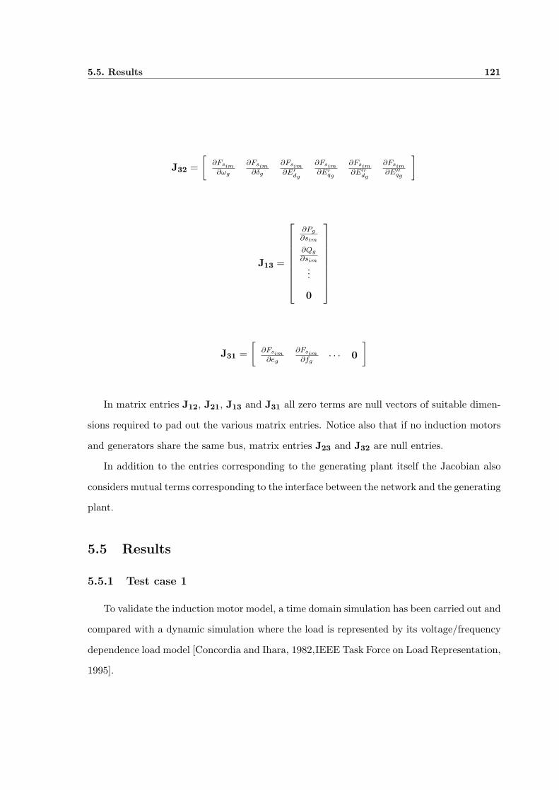
5.5. Results 121
J32 =[
∂Fsim∂ωg
∂Fsim∂δg
∂Fsim∂E′dg
∂Fsim∂E′qg
∂Fsim∂E′′dg
∂Fsim∂E′′qg
]
J13 =
∂Pg
∂sim
∂Qg
∂sim
...
0
J31 =[
∂Fsim∂eg
∂Fsim∂fg
· · · 0
]
In matrix entries J12, J21, J13 and J31 all zero terms are null vectors of suitable dimen-
sions required to pad out the various matrix entries. Notice also that if no induction motors
and generators share the same bus, matrix entries J23 and J32 are null entries.
In addition to the entries corresponding to the generating plant itself the Jacobian also
considers mutual terms corresponding to the interface between the network and the generating
plant.
5.5 Results
5.5.1 Test case 1
To validate the induction motor model, a time domain simulation has been carried out and
compared with a dynamic simulation where the load is represented by its voltage/frequency
dependence load model [Concordia and Ihara, 1982,IEEE Task Force on Load Representation,
1995].
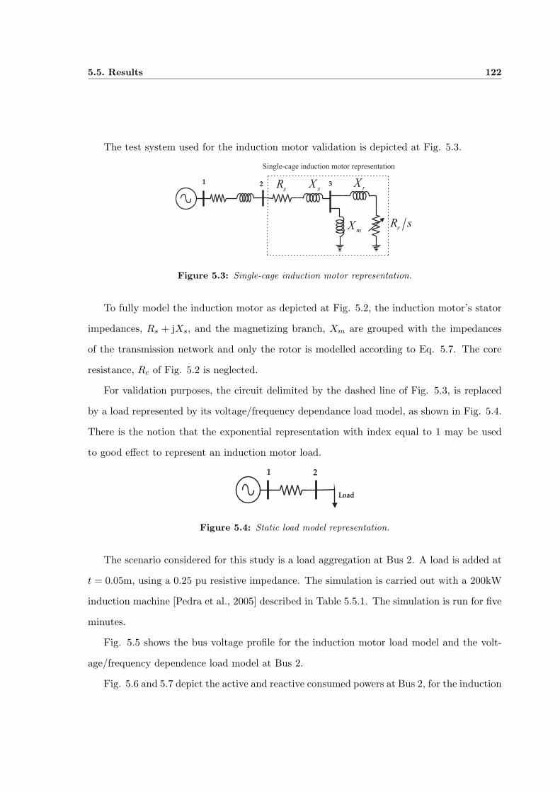
5.5. Results 122
The test system used for the induction motor validation is depicted at Fig. 5.3.
2 3
Single-cage induction motor representation
sR
sX
rR s
rX
mX
1
Figure 5.3: Single-cage induction motor representation.
To fully model the induction motor as depicted at Fig. 5.2, the induction motor’s stator
impedances, Rs + jXs, and the magnetizing branch, Xm are grouped with the impedances
of the transmission network and only the rotor is modelled according to Eq. 5.7. The core
resistance, Rc of Fig. 5.2 is neglected.
For validation purposes, the circuit delimited by the dashed line of Fig. 5.3, is replaced
by a load represented by its voltage/frequency dependance load model, as shown in Fig. 5.4.
There is the notion that the exponential representation with index equal to 1 may be used
to good effect to represent an induction motor load.
1 2
Load
Figure 5.4: Static load model representation.
The scenario considered for this study is a load aggregation at Bus 2. A load is added at
t = 0.05m, using a 0.25 pu resistive impedance. The simulation is carried out with a 200kW
induction machine [Pedra et al., 2005] described in Table 5.5.1. The simulation is run for five
minutes.
Fig. 5.5 shows the bus voltage profile for the induction motor load model and the volt-
age/frequency dependence load model at Bus 2.
Fig. 5.6 and 5.7 depict the active and reactive consumed powers at Bus 2, for the induction
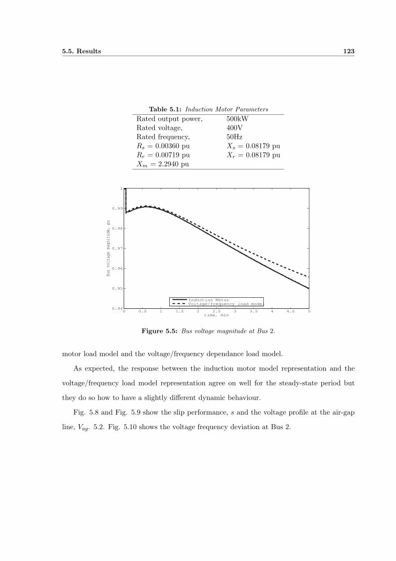
5.5. Results 123
Table 5.1: Induction Motor ParametersRated output power, 500kWRated voltage, 400VRated frequency, 50HzRs = 0.00360 pu Xs = 0.08179 puRr = 0.00719 pu Xr = 0.08179 puXm = 2.2940 pu
0 0.5 1 1.5 2 2.5 3 3.5 4 4.5 50.94
0.95
0.96
0.97
0.98
0.99
1
time, min
Bus voltage magnitude, pu
Induction MotorVoltage/frequency load model
Figure 5.5: Bus voltage magnitude at Bus 2.
motor load model and the voltage/frequency dependance load model.
As expected, the response between the induction motor model representation and the
voltage/frequency load model representation agree on well for the steady-state period but
they do so how to have a slightly different dynamic behaviour.
Fig. 5.8 and Fig. 5.9 show the slip performance, s and the voltage profile at the air-gap
line, Vag. 5.2. Fig. 5.10 shows the voltage frequency deviation at Bus 2.

5.5. Results 124
0 0.5 1 1.5 2 2.5 3 3.5 4 4.5 5
0.35
0.4
0.45
0.5
0.55
0.6
0.65
time, min
Acti
ve p
ower
, pu
Induction Motor
Voltage/frequency load model
Figure 5.6: Active power injection at Bus 2.
0 0.5 1 1.5 2 2.5 3 3.5 4 4.5 50.178
0.179
0.18
0.181
0.182
0.183
0.184
0.185
0.186
0.187
0.188
time, min
Reac
tive
pow
er,
pu
Voltage/frequency load modelInduction Motor
Figure 5.7: Reactive power injection at Bus 2.
5.5.2 Test case 2
The dynamic behaviour of the induction motor is assessed more fully. The test system
used is the nine-bus, three-machine power system depicted at Fig. 4.16 [Chow, 1982,Anderson
and Fouad, 1997].
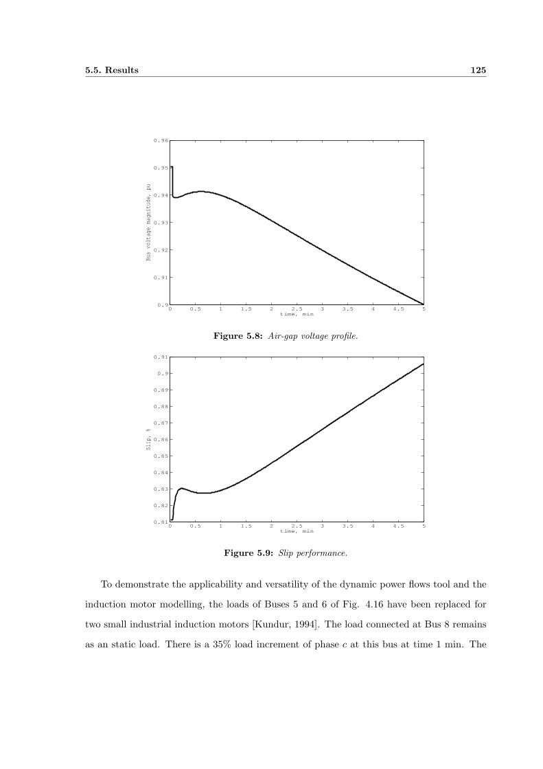
5.5. Results 125
0 0.5 1 1.5 2 2.5 3 3.5 4 4.5 50.9
0.91
0.92
0.93
0.94
0.95
0.96
time, min
Bus voltage magnitude, pu
Figure 5.8: Air-gap voltage profile.
0 0.5 1 1.5 2 2.5 3 3.5 4 4.5 50.81
0.82
0.83
0.84
0.85
0.86
0.87
0.88
0.89
0.9
0.91
time, min
Slip
, %
Figure 5.9: Slip performance.
To demonstrate the applicability and versatility of the dynamic power flows tool and the
induction motor modelling, the loads of Buses 5 and 6 of Fig. 4.16 have been replaced for
two small industrial induction motors [Kundur, 1994]. The load connected at Bus 8 remains
as an static load. There is a 35% load increment of phase c at this bus at time 1 min. The
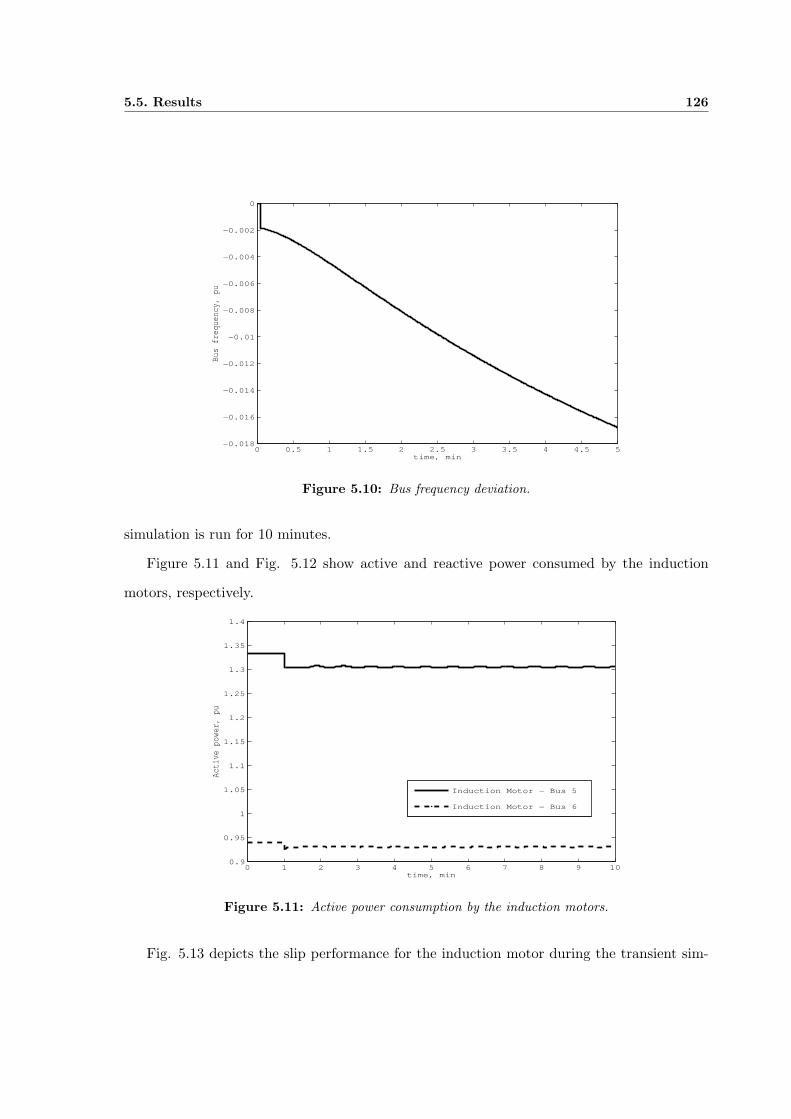
5.5. Results 126
0 0.5 1 1.5 2 2.5 3 3.5 4 4.5 5−0.018
−0.016
−0.014
−0.012
−0.01
−0.008
−0.006
−0.004
−0.002
0
time, min
Bus
freq
uenc
y, p
u
Figure 5.10: Bus frequency deviation.
simulation is run for 10 minutes.
Figure 5.11 and Fig. 5.12 show active and reactive power consumed by the induction
motors, respectively.
0 1 2 3 4 5 6 7 8 9 100.9
0.95
1
1.05
1.1
1.15
1.2
1.25
1.3
1.35
1.4
time, min
Act
ive
pow
er, p
u
Induction Motor − Bus 5
Induction Motor − Bus 6
Figure 5.11: Active power consumption by the induction motors.
Fig. 5.13 depicts the slip performance for the induction motor during the transient sim-

5.5. Results 127
0 1 2 3 4 5 6 7 8 9 100.46
0.48
0.5
0.52
0.54
0.56
0.58
0.6
time, min
Rea
ctiv
e po
wer
, pu
Induction Motor − Bus 5Induction Motor − Bus 6
Figure 5.12: Reactive power consumption by the induction motors.
ulation.
0 1 2 3 4 5 6 7 8 9 104
4.5
5
5.5
6
6.5
time, min
Slip
, % Induction Motor − Bus 5Induction Motor − Bus 6
Figure 5.13: Slip performance.
Fig. 5.14 depicts the bus voltage magnitude at load-connected buses. The voltage magni-
tude at the induction motor-connected buses is also affected by the load variation perturbation
however, it drops less than at the affected bus, as is shown in Fig. 5.14. Due to load mod-
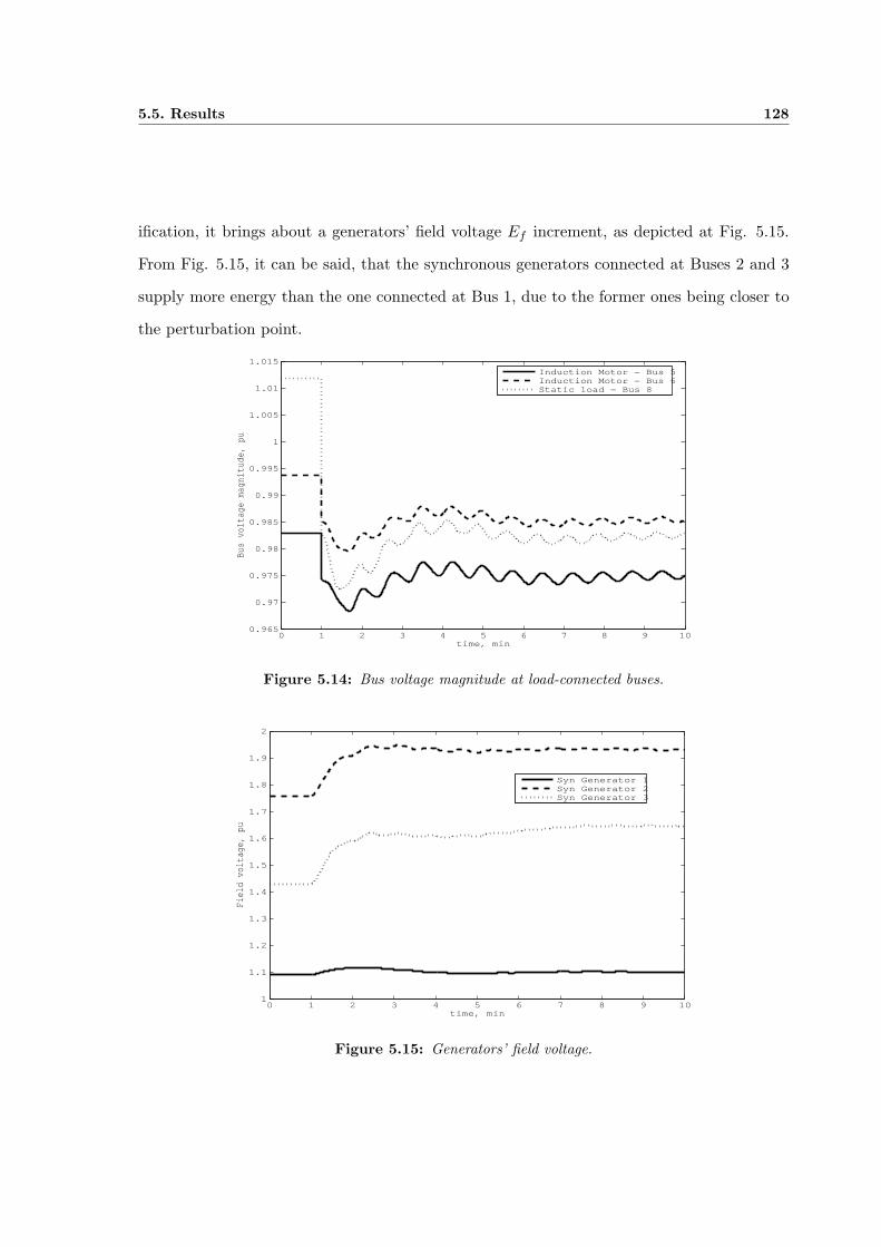
5.5. Results 128
ification, it brings about a generators’ field voltage Ef increment, as depicted at Fig. 5.15.
From Fig. 5.15, it can be said, that the synchronous generators connected at Buses 2 and 3
supply more energy than the one connected at Bus 1, due to the former ones being closer to
the perturbation point.
0 1 2 3 4 5 6 7 8 9 100.965
0.97
0.975
0.98
0.985
0.99
0.995
1
1.005
1.01
1.015
time, min
Bus
vol
tage
mag
nitu
de, p
u
Induction Motor − Bus 5Induction Motor − Bus 6Static load − Bus 8
Figure 5.14: Bus voltage magnitude at load-connected buses.
0 1 2 3 4 5 6 7 8 9 101
1.1
1.2
1.3
1.4
1.5
1.6
1.7
1.8
1.9
2
time, min
Fiel
d vo
ltag
e, p
u
Syn Generator 1Syn Generator 2Syn Generator 3
Figure 5.15: Generators’ field voltage.
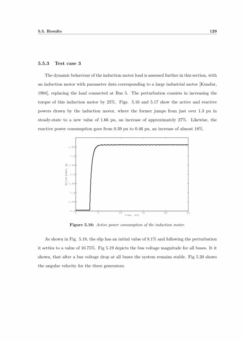
5.5. Results 129
5.5.3 Test case 3
The dynamic behaviour of the induction motor load is assessed further in this section, with
an induction motor with parameter data corresponding to a large industrial motor [Kundur,
1994], replacing the load connected at Bus 5. The perturbation consists in increasing the
torque of this induction motor by 25%. Figs. 5.16 and 5.17 show the active and reactive
powers drawn by the induction motor, where the former jumps from just over 1.3 pu in
steady-state to a new value of 1.66 pu, an increase of approximately 27%. Likewise, the
reactive power consumption goes from 0.39 pu to 0.46 pu, an increase of almost 18%.
0 5 10 15 20 251.3
1.35
1.4
1.45
1.5
1.55
1.6
1.65
time, min
Active power, pu
Figure 5.16: Active power consumption of the induction motor.
As shown in Fig. 5.18, the slip has an initial value of 8.1% and following the perturbation
it settles to a value of 10.75%. Fig 5.19 depicts the bus voltage magnitude for all buses. It it
shown, that after a bus voltage drop at all buses the system remains stable. Fig 5.20 shows
the angular velocity for the three generators.
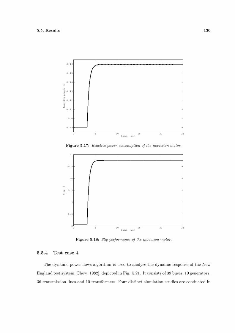
5.5. Results 130
0 5 10 15 20 25
0.39
0.4
0.41
0.42
0.43
0.44
0.45
0.46
time, min
Reactive power, pu
Figure 5.17: Reactive power consumption of the induction motor.
0 5 10 15 20 258
8.5
9
9.5
10
10.5
11
time, min
Slip
, %
Figure 5.18: Slip performance of the induction motor.
5.5.4 Test case 4
The dynamic power flows algorithm is used to analyse the dynamic response of the New
England test system [Chow, 1982], depicted in Fig. 5.21. It consists of 39 buses, 10 generators,
36 transmission lines and 10 transformers. Four distinct simulation studies are conducted in
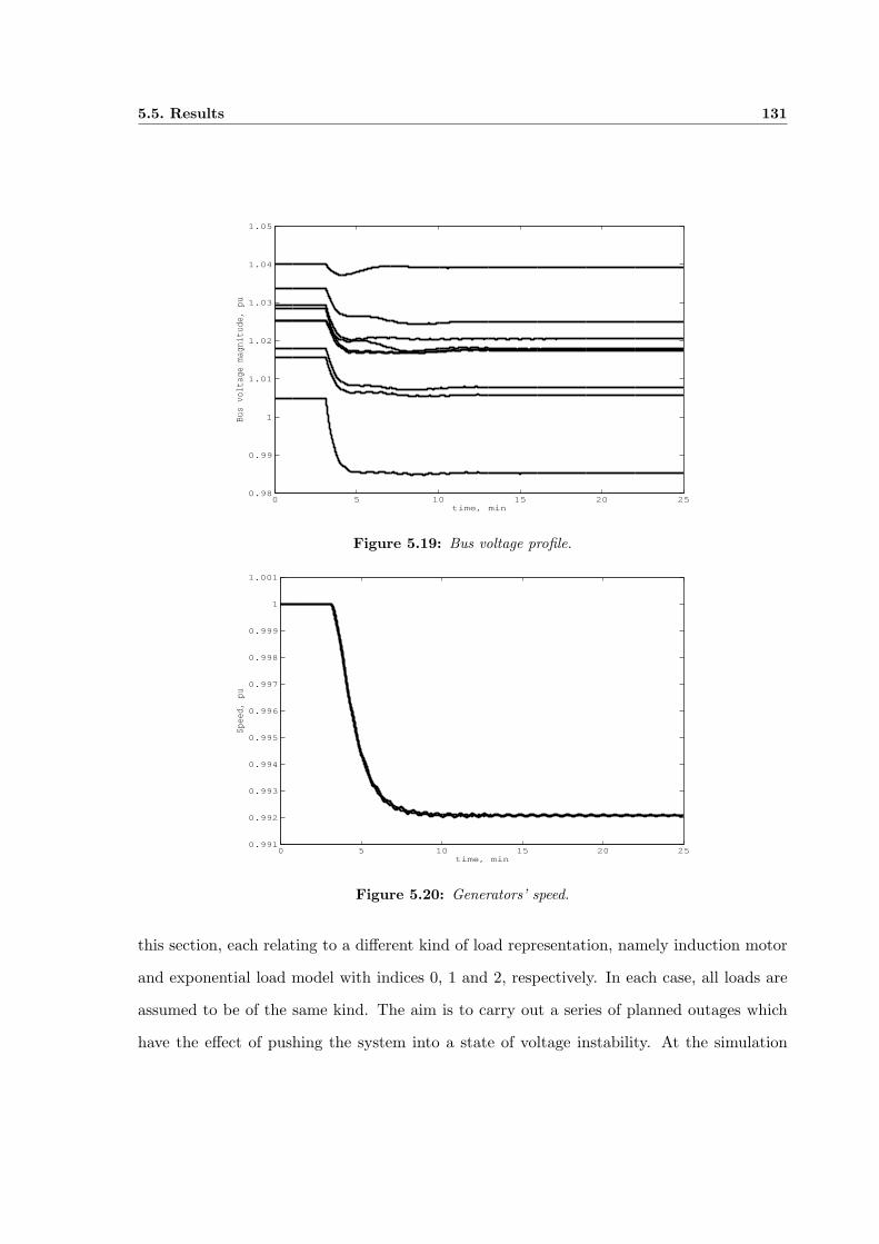
5.5. Results 131
0 5 10 15 20 250.98
0.99
1
1.01
1.02
1.03
1.04
1.05
time, min
Bus
volt
age
magn
itud
e, p
u
Figure 5.19: Bus voltage profile.
0 5 10 15 20 250.991
0.992
0.993
0.994
0.995
0.996
0.997
0.998
0.999
1
1.001
time, min
Spee
d, p
u
Figure 5.20: Generators’ speed.
this section, each relating to a different kind of load representation, namely induction motor
and exponential load model with indices 0, 1 and 2, respectively. In each case, all loads are
assumed to be of the same kind. The aim is to carry out a series of planned outages which
have the effect of pushing the system into a state of voltage instability. At the simulation
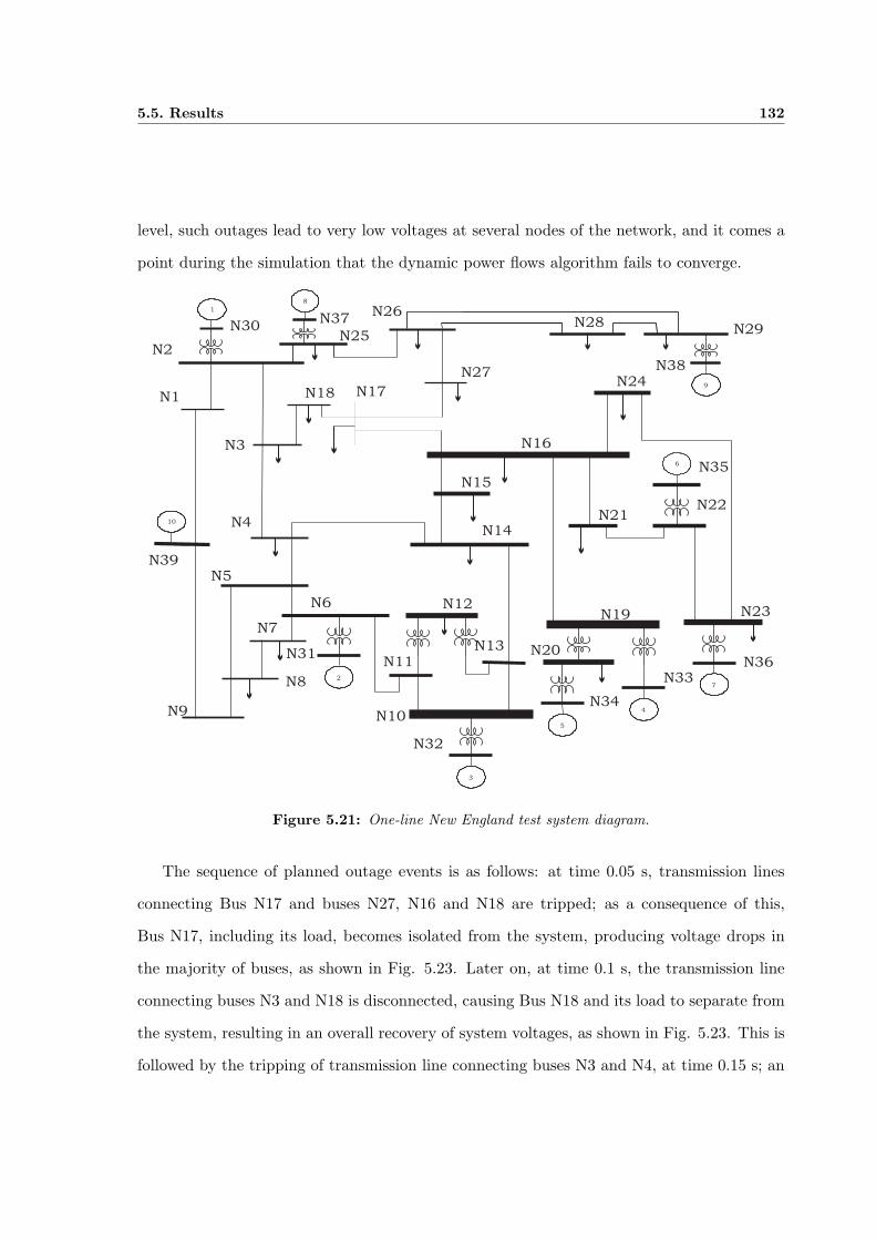
5.5. Results 132
level, such outages lead to very low voltages at several nodes of the network, and it comes a
point during the simulation that the dynamic power flows algorithm fails to converge.
N30N37
N38
9
8
10
N2
N25
N26N28
N29
1
2
3
5
4
7
N1 N18 N17
N27
N3
N39
N4
N5
N6
N7
N8
N9
N31
N12
N11
N10
N13
N32
N34
N20
N19
N33
N36
N23
N21N22
N356
N15
N16
N24
N14
Figure 5.21: One-line New England test system diagram.
The sequence of planned outage events is as follows: at time 0.05 s, transmission lines
connecting Bus N17 and buses N27, N16 and N18 are tripped; as a consequence of this,
Bus N17, including its load, becomes isolated from the system, producing voltage drops in
the majority of buses, as shown in Fig. 5.23. Later on, at time 0.1 s, the transmission line
connecting buses N3 and N18 is disconnected, causing Bus N18 and its load to separate from
the system, resulting in an overall recovery of system voltages, as shown in Fig. 5.23. This is
followed by the tripping of transmission line connecting buses N3 and N4, at time 0.15 s; an

5.5. Results 133
event which to a greater or lesser extent reduces voltages at all buses. This trend accentuates
with time and in several buses, when the system load is represented by induction motors, the
voltages drop below 0.93 p.u. at a time 0.25 s. Just after 0.42 s, the voltage at Bus N14, which
has shown to be the weakest bus, reaches a value of 0.85 p.u. and the dynamic power flows
algorithm can not reach convergence any longer. The results in Fig. 5.22 corresponds to the
case when all loads are assumed to be induction motors with parameter data corresponding
to a large industrial motor [Kundur, 1994].
0 0.05 0.1 0.15 0.2 0.25 0.3 0.35 0.4
0.85
0.9
0.95
1
1.05
1.1
time, sec
Bus
volt
age
magn
itud
e, p
u
Figure 5.22: Bus voltage profile - Loads as induction motors.
In Fig. 5.23 it is shown how the overall system voltage perform when the load is expo-
nential with index 1. The simulation seems to be slightly more robust with the static load
representation with exponential index 1 than with the dynamic load representation; the sim-
ulation runs for almost 0.50 s but the downward trend of system voltage is very much in line
with that observed in Fig. 5.22 for the case of induction motor load. A more detailed assess-
ment is made with reference to Fig. 5.26, where nodal voltages are shown for Bus N14; the
weakest bus in the network. Four different results are shown, corresponding to the four kinds
of load representation used in the study. At this particular bus, the dynamic load voltage
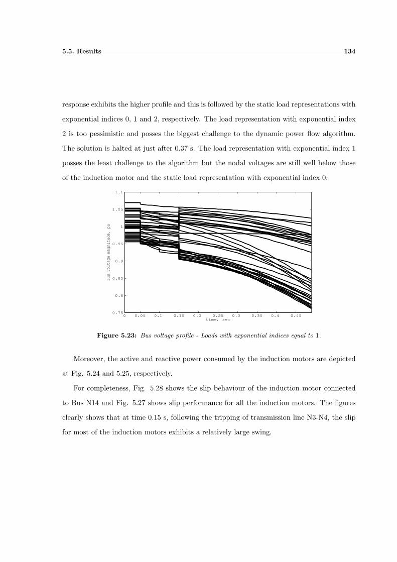
5.5. Results 134
response exhibits the higher profile and this is followed by the static load representations with
exponential indices 0, 1 and 2, respectively. The load representation with exponential index
2 is too pessimistic and posses the biggest challenge to the dynamic power flow algorithm.
The solution is halted at just after 0.37 s. The load representation with exponential index 1
posses the least challenge to the algorithm but the nodal voltages are still well below those
of the induction motor and the static load representation with exponential index 0.
0 0.05 0.1 0.15 0.2 0.25 0.3 0.35 0.4 0.450.75
0.8
0.85
0.9
0.95
1
1.05
1.1
time, sec
Bus
volt
age
magn
itud
e, p
u
Figure 5.23: Bus voltage profile - Loads with exponential indices equal to 1.
Moreover, the active and reactive power consumed by the induction motors are depicted
at Fig. 5.24 and 5.25, respectively.
For completeness, Fig. 5.28 shows the slip behaviour of the induction motor connected
to Bus N14 and Fig. 5.27 shows slip performance for all the induction motors. The figures
clearly shows that at time 0.15 s, following the tripping of transmission line N3-N4, the slip
for most of the induction motors exhibits a relatively large swing.
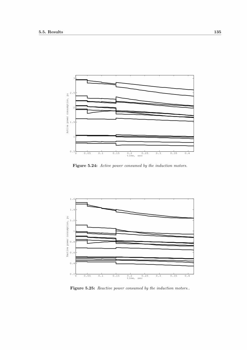
5.5. Results 135
0 0.05 0.1 0.15 0.2 0.25 0.3 0.35 0.4 0.5
1
1.5
2
2.5
3
time, sec
Active power consumption, pu
Figure 5.24: Active power consumed by the induction motors.
0 0.05 0.1 0.15 0.2 0.25 0.3 0.35 0.4 0.2
0.4
0.6
0.8
1
1.2
1.4
1.6
time, sec
Ract
ive
powe
r co
nsum
ptio
n, p
u
Figure 5.25: Reactive power consumed by the induction motors..
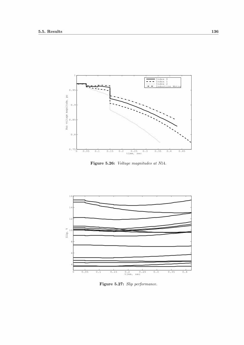
5.5. Results 136
0 0.05 0.1 0.15 0.2 0.25 0.3 0.35 0.4 0.450.75
0.8
0.85
0.9
0.95
1
time, sec
Bus
volt
age
magn
itud
e, p
u
Index 0Index 1Index 2Induction Motor
Figure 5.26: Voltage magnitudes at N14.
0 0.05 0.1 0.15 0.2 0.25 0.3 0.35 0.4
4
6
8
10
12
14
16
time, sec
Slip
, %
Figure 5.27: Slip performance.

5.5. Results 137
0 0.05 0.1 0.15 0.2 0.25 0.3 0.35 0.4 3.63
3.64
3.65
3.66
3.67
3.68
3.69
3.7
3.71
3.72
time, sec
Slip
, %
Indu
ctio
n Mo
tor
conn
ecte
d at
Bus
N14
Figure 5.28: Slip performance.
5.6. Summary 138
5.6 Summary
This chapter relies mainly, on the development, analyses and implementation of the loads’
behaviour in a dynamic power flow algorithm.
The dynamic power flows computer program has been extended to encompass static and
dynamic load modelling including induction motor loads, to enable the study of a wide range
of dynamic voltage phenomena in power systems. The upgraded software is well suited to
carrying out comprehensive studies of wide-area dynamic voltage collapse, as demonstrated by
numerical example. The overall method blends seamlessly the algebraic-differential equation
set which represent the power system by using repeated linearization and the trapezoidal rule,
resulting in a unified frame-of-reference with which to carry out reliable numerical solutions
using the Newton-Raphson method.
In a nutshell, this is a dynamic power flows algorithm which enables dynamic assessments
of the power system, with strong convergence characteristics and flexible network representa-
tion. Besides presenting a detailed description of how high-order synchronous generator and
induction motor models are incorporated into the dynamic power flows algorithm, the thrust
of this chapter is on system load modelling, and the responses of static load representations
are compared with those of induction motors, and general conclusions are drawn.
Chapter 6
Modelling of FACTS Controllers
6.1 Introduction
Voltage stability and control are increasingly becoming a limiting factor in the planning
and operation of power systems, mainly in weakly interconnected ones. However, for a num-
ber of economical and environmental reasons the construction of new transmission lines is
suffering delays. This has resulted in the need to maximise the use of existing transmission
facilities. During steady state operation, bus voltages must be controlled on a specified range.
A suitable voltage and reactive power control allows to obtain important benefits in the power
system operation, such as reduction of voltage gradients, efficient transmission capacity util-
isation and increase of stability margins. Applying various control equipment and methods,
the voltage control objectives in transmission system can be achieved. Some controllers work
on the basis of injecting a series voltage injection an others on injecting a shunt reactive
current at the point of connection with the power system. Following a disturbance, changes
in the system voltage take place and restoration to the reference values depends very much on
the dynamic response of the excitation systems and the other voltage controllers. In the last
decade commercial availability of Gate Turn-Off thyristor (GTO) devices with high power
handling capability, and the rapid progress of other power-semiconductor devices such as
6.2. Static Synchronous Compensator (STATCOM) 140
IGBT, have led to the development of controllable reactive power sources utilising electronic
switching converter technology [Nabavi-Niaki, 1996]. These technologies offer considerable
advantages over the existing ones such as static VAR compensators in terms of smaller foot-
prints and operational performance. GTOs and IGBTs enable the design of solid-state shunt
reactive compensation equipment based upon switching converter technology.
The advent of Flexible AC Transmission Systems (FACTS) has given rise to a new family
of power electronic equipment for controlling and optimising the performance of a power
system, e.g. STATCOM, SSSC and UPFC. The voltage-source converter (VSC) is widely
accepted to be the next generation of reactive power controller to the SVC, made up by
thyristor-switched capacitors (TSC) and thyristor controlled reactors (TCR).
Researchers are directing their efforts at the application of FACTS to enhance the eco-
nomic operational and the dynamic response of the power system. The major areas of dy-
namic applications are: voltage stability enhancement, damping torsional oscillations, power
system voltage control, and power system stability improvement. These applications re-
quire of suitable control schemes implementation (voltage magnitude and phase angle con-
trol) [Banerjee and Verghese, 2001,Kassakian et al., 1991, IEEE, 2000].
6.2 Static Synchronous Compensator (STATCOM)
The Static Synchronous Compensator (STATCOM) is a shunt connected reactive compen-
sator capable of generating or absorbing reactive power in a dynamic fashion. The STATCOM
possesses operating characteristics similar to those of the rotating synchronous compensator
but with no mechanical inertia. The STATCOM employs solid state power switching devices,
providing rapid controllability of the voltage magnitude.
The STATCOM contains a step-down transformer, with a leakage reactance, a GTO or
IGBT voltage source inverter (VSI), a DC capacitor and a control structure. The AC voltage
difference across the leakage reactance is regulated to produced reactive power exchange
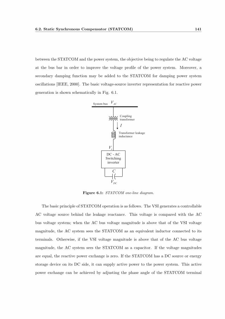
6.2. Static Synchronous Compensator (STATCOM) 141
between the STATCOM and the power system, the objective being to regulate the AC voltage
at the bus bar in order to improve the voltage profile of the power system. Moreover, a
secondary damping function may be added to the STATCOM for damping power system
oscillations [IEEE, 2000]. The basic voltage-source inverter representation for reactive power
generation is shown schematically in Fig. 6.1.
sV
ACV
I
DC - AC
Switching
inverter
Coupling
transformer
Transformer leakage
inductance
DCV
C
System bus
Figure 6.1: STATCOM one-line diagram.
The basic principle of STATCOM operation is as follows. The VSI generates a controllable
AC voltage source behind the leakage reactance. This voltage is compared with the AC
bus voltage system; when the AC bus voltage magnitude is above that of the VSI voltage
magnitude, the AC system sees the STATCOM as an equivalent inductor connected to its
terminals. Otherwise, if the VSI voltage magnitude is above that of the AC bus voltage
magnitude, the AC system sees the STATCOM as a capacitor. If the voltage magnitudes
are equal, the reactive power exchange is zero. If the STATCOM has a DC source or energy
storage device on its DC side, it can supply active power to the power system. This active
power exchange can be achieved by adjusting the phase angle of the STATCOM terminal

6.2. Static Synchronous Compensator (STATCOM) 142
and the phase angle of the AC power system. When the phase angle of the AC power system
leads the VSI phase angle, the STATCOM absorbs active power from the AC system; if the
phase angle of the AC power system lags the VSI phase angle, the STATCOM supplies active
power to AC system [Padiyar and Kulkarni, 1997,Lehn and Iravani, 1998,Lehn and Iravani,
2002]. Typical applications of the STATCOM are:
• Effective voltage regulation and control,
• Reduction of temporary overvoltages,
• Improvement of steady-state power transfer capacity
• Improvement of transient stability margin,
• Damping of power system oscillations,
• Damping of subsynchronous power system oscillations,
• Flicker control,
• Power quality improvement,
The voltage source converter is the building block of a STATCOM and other FACTS
devices. A simple two-level converter produces a square voltage waveform as it switches the
direct voltage source on and off. The basic objective of a VSC is to produce a sinusoidal
AC voltage with minimal harmonic distortion from a DC voltage. Three basic techniques
are used for reducing harmonics in the converter output voltage. Harmonic neutralisation
using magnetic coupling (multi-pulse converter configurations), harmonic reduction using
multi-level converter configurations and control.
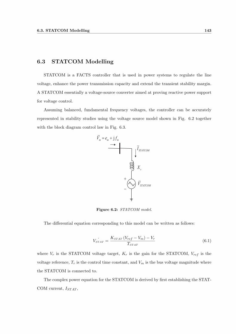
6.3. STATCOM Modelling 143
6.3 STATCOM Modelling
STATCOM is a FACTS controller that is used in power systems to regulate the line
voltage, enhance the power transmission capacity and extend the transient stability margin.
A STATCOM essentially a voltage-source converter aimed at proving reactive power support
for voltage control.
Assuming balanced, fundamental frequency voltages, the controller can be accurately
represented in stability studies using the voltage source model shown in Fig. 6.2 together
with the block diagram control law in Fig. 6.3.
STATCOMV
sX
jm m m
V e f= +
-
+
STATCOMI
Figure 6.2: STATCOM model.
The differential equation corresponding to this model can be written as follows:
˙VSTAT =KSTAT (Vref − Vm)− Vr
TSTAT
(6.1)
where Vr is the STATCOM voltage target, Kr is the gain for the STATCOM, Vref is the
voltage reference, Tr is the control time constant, and Vm is the bus voltage magnitude where
the STATCOM is connected to.
The complex power equation for the STATCOM is derived by first establishing the STAT-
COM current, ISTAT ,
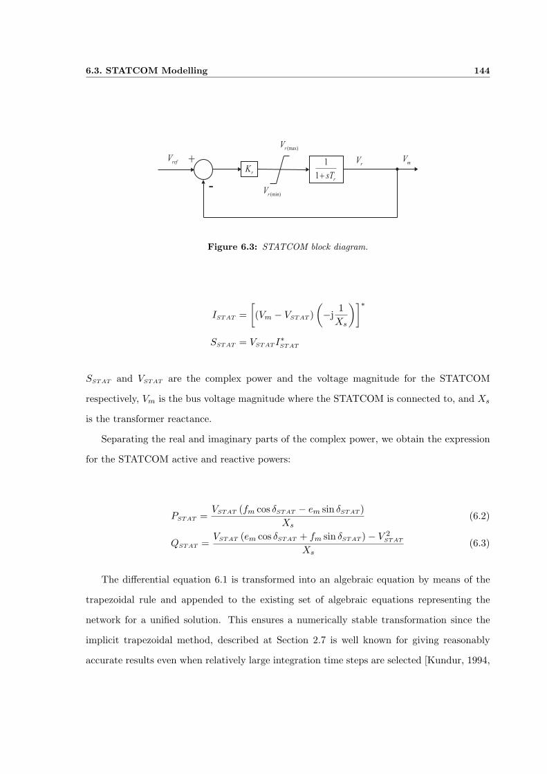
6.3. STATCOM Modelling 144
+
-
1
1r
sT+r
Kr
V mV
(min)rV
(max)rV
refV
Figure 6.3: STATCOM block diagram.
ISTAT =[(Vm − VSTAT )
(−j
1Xs
)]∗
SSTAT = VSTAT I∗STAT
SSTAT and VSTAT are the complex power and the voltage magnitude for the STATCOM
respectively, Vm is the bus voltage magnitude where the STATCOM is connected to, and Xs
is the transformer reactance.
Separating the real and imaginary parts of the complex power, we obtain the expression
for the STATCOM active and reactive powers:
PSTAT =VSTAT (fm cos δSTAT − em sin δSTAT )
Xs(6.2)
QSTAT =VSTAT (em cos δSTAT + fm sin δSTAT )− V 2
STAT
Xs(6.3)
The differential equation 6.1 is transformed into an algebraic equation by means of the
trapezoidal rule and appended to the existing set of algebraic equations representing the
network for a unified solution. This ensures a numerically stable transformation since the
implicit trapezoidal method, described at Section 2.7 is well known for giving reasonably
accurate results even when relatively large integration time steps are selected [Kundur, 1994,
6.3. STATCOM Modelling 145
Machowski et al., 1997].
The trapezoidal method is applied to the differential Eq. 6.1 as follows,
VSTAT (t) − VSTAT (t−∆t) =
∆t
2 TSTAT
[KSTAT
(Vref − Vm(t)
)− VSTAT (t) +(Vref − Vm(t−∆t)
)− VSTAT (t−∆t)
](6.4)
Re-arranging terms, leads to a more compact expression,
FSTAT = FSTAT (t) + FSTAT (t−∆t) + CSTAT = 0
where
FSTAT (t) = VSTAT (t)
[1− ∆t
2 TSTAT
]− ∆t
2 TSTAT
KSTAT Vm(t)
FSTAT (t−∆t) = −VSTAT (t−∆t)
[1− ∆t
2 TSTAT
]− ∆t
2 TSTAT
KSTAT Vm(t−∆t)
CSTAT =∆t
TSTAT
KSTAT Vref
Equation 6.2 and Eq. 6.3, describing the active and reactive powers contributions for the
STATCOM, are explicitly incorporated into the active and reactive powers injected in the
network buses and the powers contributed by all generators in the network:
Pk + Pe,l + PSTAT,m
Qk + Qe,l + QSTAT,m
(6.5)
for k = 1, . . . , l, . . . , nbus, l = 1, . . . , ngen and m = 1, . . . , nSTAT .
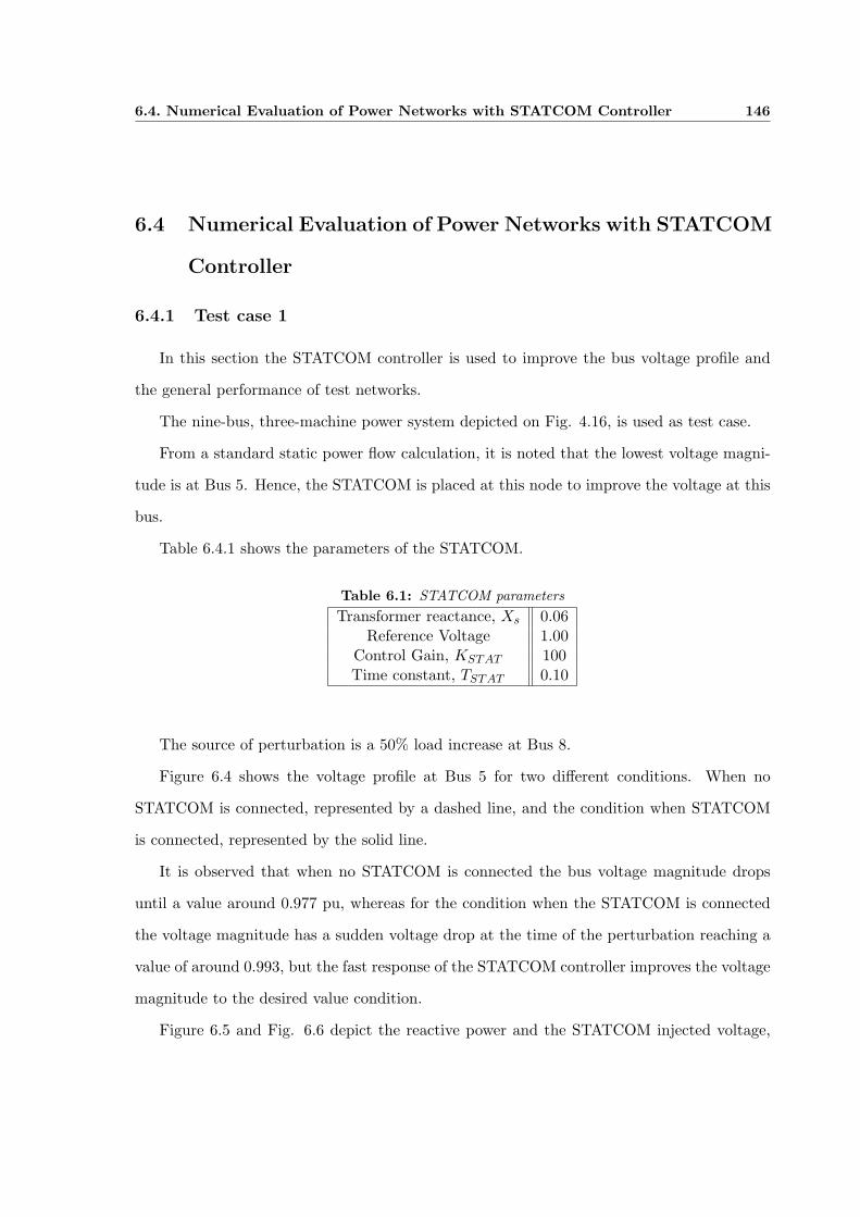
6.4. Numerical Evaluation of Power Networks with STATCOM Controller 146
6.4 Numerical Evaluation of Power Networks with STATCOM
Controller
6.4.1 Test case 1
In this section the STATCOM controller is used to improve the bus voltage profile and
the general performance of test networks.
The nine-bus, three-machine power system depicted on Fig. 4.16, is used as test case.
From a standard static power flow calculation, it is noted that the lowest voltage magni-
tude is at Bus 5. Hence, the STATCOM is placed at this node to improve the voltage at this
bus.
Table 6.4.1 shows the parameters of the STATCOM.
Table 6.1: STATCOM parametersTransformer reactance, Xs 0.06
Reference Voltage 1.00Control Gain, KSTAT 100Time constant, TSTAT 0.10
The source of perturbation is a 50% load increase at Bus 8.
Figure 6.4 shows the voltage profile at Bus 5 for two different conditions. When no
STATCOM is connected, represented by a dashed line, and the condition when STATCOM
is connected, represented by the solid line.
It is observed that when no STATCOM is connected the bus voltage magnitude drops
until a value around 0.977 pu, whereas for the condition when the STATCOM is connected
the voltage magnitude has a sudden voltage drop at the time of the perturbation reaching a
value of around 0.993, but the fast response of the STATCOM controller improves the voltage
magnitude to the desired value condition.
Figure 6.5 and Fig. 6.6 depict the reactive power and the STATCOM injected voltage,
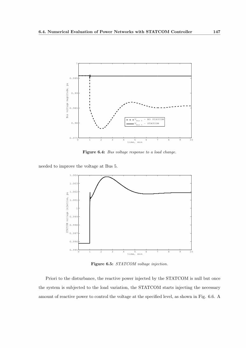
6.4. Numerical Evaluation of Power Networks with STATCOM Controller 147
0 1 2 3 4 5 6 7 8 9 100.975
0.98
0.985
0.99
0.995
1
time, min
Bus
vol
tage
mag
nitu
de, p
u
VBus 5
− NO STATCOM
VBus 5
− STATCOM
Figure 6.4: Bus voltage response to a load change.
needed to improve the voltage at Bus 5.
0 1 2 3 4 5 6 7 8 9 100.995
0.996
0.997
0.998
0.999
1
1.001
1.002
1.003
1.004
time, min
STAT
COM
volt
age
inje
ctio
n, p
u
Figure 6.5: STATCOM voltage injection.
Priori to the disturbance, the reactive power injected by the STATCOM is null but once
the system is subjected to the load variation, the STATCOM starts injecting the necessary
amount of reactive power to control the voltage at the specified level, as shown in Fig. 6.6. A
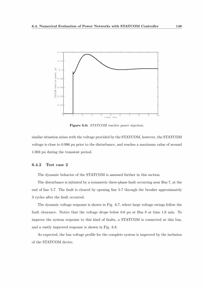
6.4. Numerical Evaluation of Power Networks with STATCOM Controller 148
0 1 2 3 4 5 6 7 8 9 100
0.02
0.04
0.06
0.08
0.1
0.12
0.14
time, min
STAT
COM
reac
tive
pow
er,
pu
Figure 6.6: STATCOM reactive power injection.
similar situation arises with the voltage provided by the STATCOM, however, the STATCOM
voltage is close to 0.996 pu prior to the disturbance, and reaches a maximum value of around
1.003 pu during the transient period.
6.4.2 Test case 2
The dynamic behavior of the STATCOM is assessed further in this section.
The disturbance is initiated by a symmetric three-phase fault occurring near Bus 7, at the
end of line 5-7. The fault is cleared by opening line 5-7 through the breaker approximately
3 cycles after the fault occurred.
The dynamic voltage response is shown in Fig. 6.7, where large voltage swings follow the
fault clearance. Notice that the voltage drops below 0.6 pu at Bus 8 at time 1.6 min. To
improve the system response to this kind of faults, a STATCOM is connected at this bus,
and a vastly improved response is shown in Fig. 6.8.
As expected, the bus voltage profile for the complete system is improved by the inclusion
of the STATCOM device.
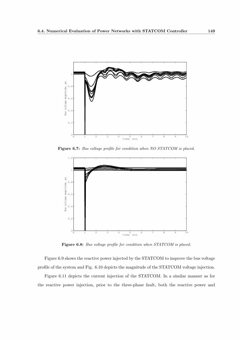
6.4. Numerical Evaluation of Power Networks with STATCOM Controller 149
0 1 2 3 4 5 6 7 8 9 100
0.2
0.4
0.6
0.8
1
time, min
Bus voltage magnitude, pu
Figure 6.7: Bus voltage profile for condition when NO STATCOM is placed.
0 1 2 3 4 5 6 7 8 9 100
0.2
0.4
0.6
0.8
1
1.2
time, min
Bus
volt
age
magn
itud
e, p
u
Figure 6.8: Bus voltage profile for condition when STATCOM is placed.
Figure 6.9 shows the reactive power injected by the STATCOM to improve the bus voltage
profile of the system and Fig. 6.10 depicts the magnitude of the STATCOM voltage injection.
Figure 6.11 depicts the current injection of the STATCOM. In a similar manner as for
the reactive power injection, prior to the three-phase fault, both the reactive power and
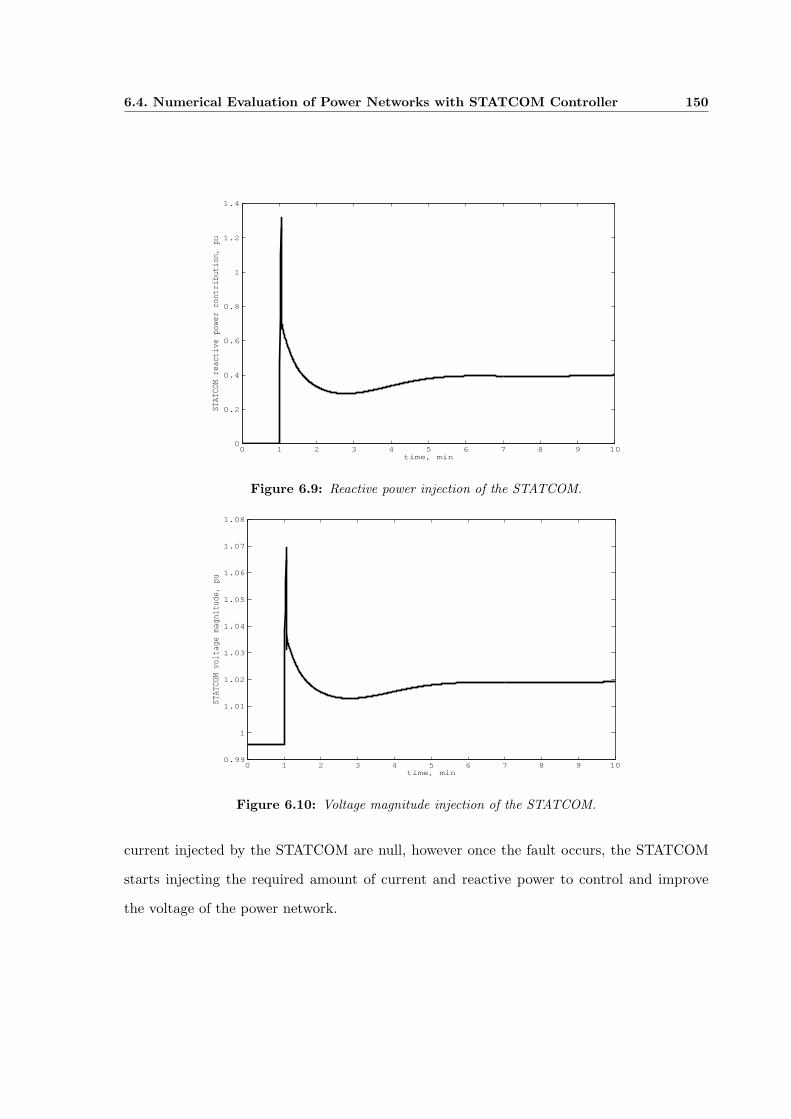
6.4. Numerical Evaluation of Power Networks with STATCOM Controller 150
0 1 2 3 4 5 6 7 8 9 100
0.2
0.4
0.6
0.8
1
1.2
1.4
time, min
STAT
COM
reac
tive
pow
er c
ontr
ibut
ion,
pu
Figure 6.9: Reactive power injection of the STATCOM.
0 1 2 3 4 5 6 7 8 9 100.99
1
1.01
1.02
1.03
1.04
1.05
1.06
1.07
1.08
time, min
STAT
COM
volt
age
magn
itud
e, p
u
Figure 6.10: Voltage magnitude injection of the STATCOM.
current injected by the STATCOM are null, however once the fault occurs, the STATCOM
starts injecting the required amount of current and reactive power to control and improve
the voltage of the power network.
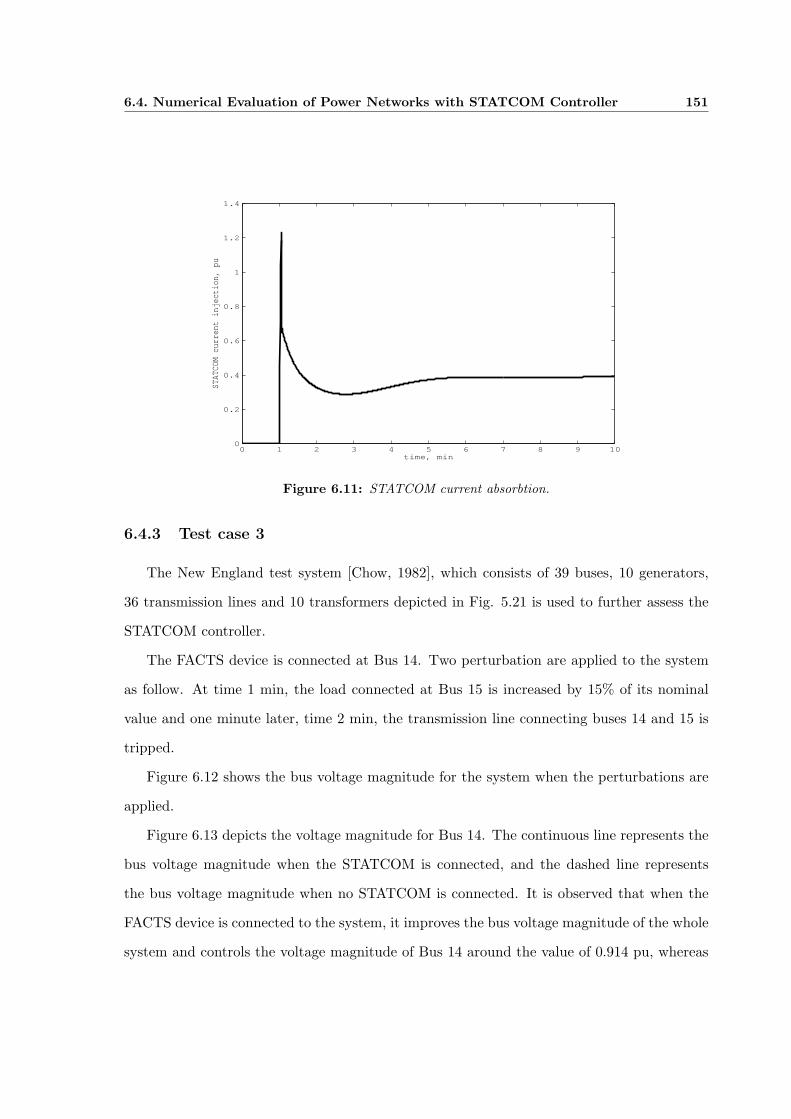
6.4. Numerical Evaluation of Power Networks with STATCOM Controller 151
0 1 2 3 4 5 6 7 8 9 100
0.2
0.4
0.6
0.8
1
1.2
1.4
time, min
STAT
COM
curr
ent
inje
ctio
n, p
u
Figure 6.11: STATCOM current absorbtion.
6.4.3 Test case 3
The New England test system [Chow, 1982], which consists of 39 buses, 10 generators,
36 transmission lines and 10 transformers depicted in Fig. 5.21 is used to further assess the
STATCOM controller.
The FACTS device is connected at Bus 14. Two perturbation are applied to the system
as follow. At time 1 min, the load connected at Bus 15 is increased by 15% of its nominal
value and one minute later, time 2 min, the transmission line connecting buses 14 and 15 is
tripped.
Figure 6.12 shows the bus voltage magnitude for the system when the perturbations are
applied.
Figure 6.13 depicts the voltage magnitude for Bus 14. The continuous line represents the
bus voltage magnitude when the STATCOM is connected, and the dashed line represents
the bus voltage magnitude when no STATCOM is connected. It is observed that when the
FACTS device is connected to the system, it improves the bus voltage magnitude of the whole
system and controls the voltage magnitude of Bus 14 around the value of 0.914 pu, whereas
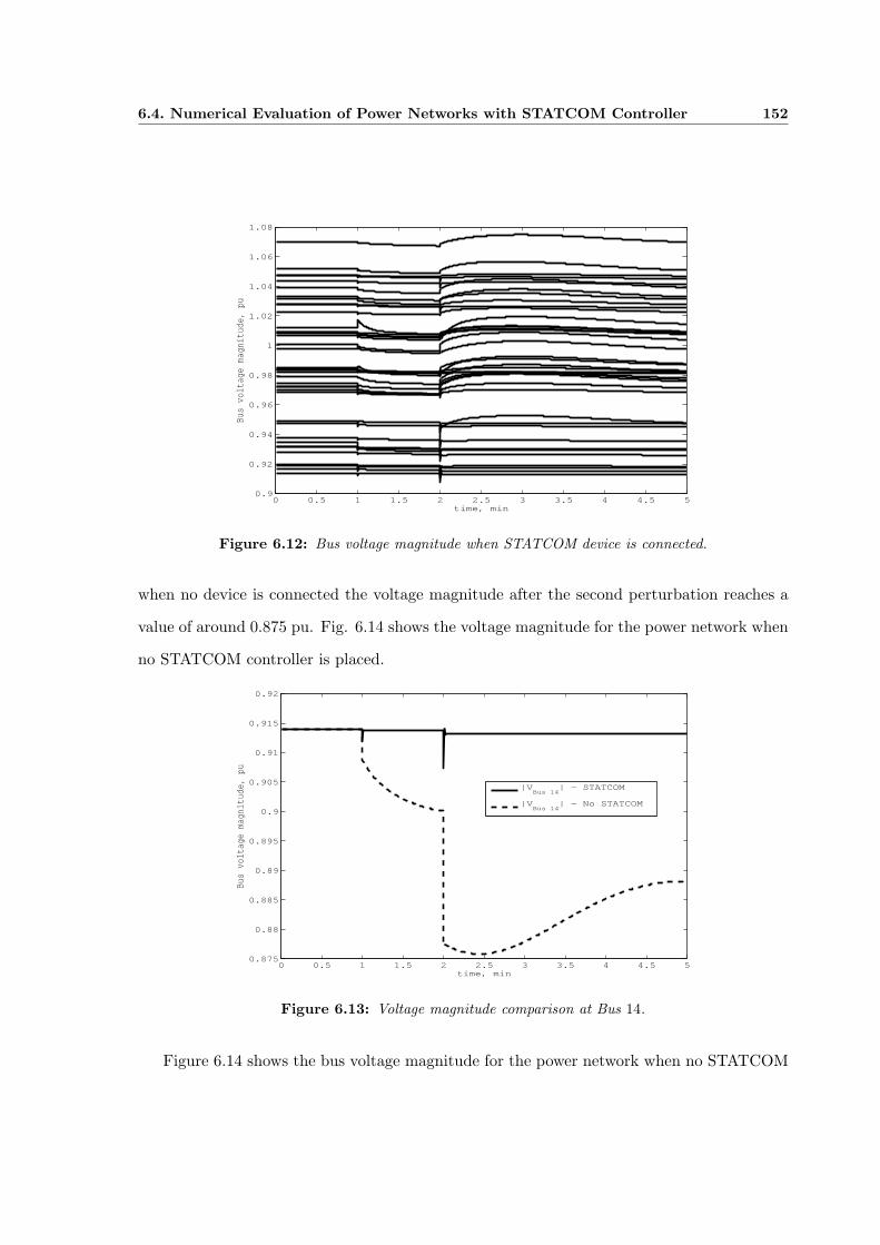
6.4. Numerical Evaluation of Power Networks with STATCOM Controller 152
0 0.5 1 1.5 2 2.5 3 3.5 4 4.5 50.9
0.92
0.94
0.96
0.98
1
1.02
1.04
1.06
1.08
time, min
Bus voltage magnitude, pu
Figure 6.12: Bus voltage magnitude when STATCOM device is connected.
when no device is connected the voltage magnitude after the second perturbation reaches a
value of around 0.875 pu. Fig. 6.14 shows the voltage magnitude for the power network when
no STATCOM controller is placed.
0 0.5 1 1.5 2 2.5 3 3.5 4 4.5 50.875
0.88
0.885
0.89
0.895
0.9
0.905
0.91
0.915
0.92
time, min
Bus
vol
tage
mag
nitu
de, p
u
|VBus 14
| − STATCOM
|VBus 14
| − No STATCOM
Figure 6.13: Voltage magnitude comparison at Bus 14.
Figure 6.14 shows the bus voltage magnitude for the power network when no STATCOM
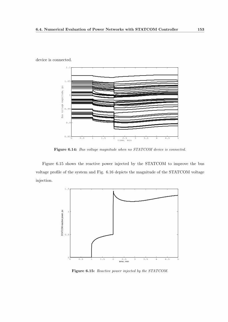
6.4. Numerical Evaluation of Power Networks with STATCOM Controller 153
device is connected.
0 0.5 1 1.5 2 2.5 3 3.5 4 4.5 50.85
0.9
0.95
1
1.05
1.1
time, min
Bus
volt
age
magn
itud
e, p
u
Figure 6.14: Bus voltage magnitude when no STATCOM device is connected.
Figure 6.15 shows the reactive power injected by the STATCOM to improve the bus
voltage profile of the system and Fig. 6.16 depicts the magnitude of the STATCOM voltage
injection.
0 0.5 1 1.5 2 2.5 3 3.5 4 4.5 50
0.5
1
1.5
time, min
STAT
CO
M re
activ
e po
wer
, pu
Figure 6.15: Reactive power injected by the STATCOM.
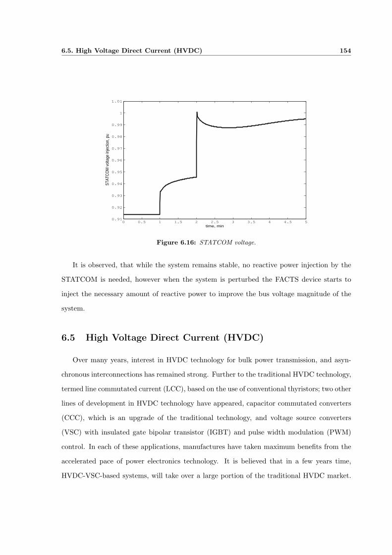
6.5. High Voltage Direct Current (HVDC) 154
0 0.5 1 1.5 2 2.5 3 3.5 4 4.5 50.91
0.92
0.93
0.94
0.95
0.96
0.97
0.98
0.99
1
1.01
time, min
STAT
CO
M v
olta
ge in
ject
ion,
pu
Figure 6.16: STATCOM voltage.
It is observed, that while the system remains stable, no reactive power injection by the
STATCOM is needed, however when the system is perturbed the FACTS device starts to
inject the necessary amount of reactive power to improve the bus voltage magnitude of the
system.
6.5 High Voltage Direct Current (HVDC)
Over many years, interest in HVDC technology for bulk power transmission, and asyn-
chronous interconnections has remained strong. Further to the traditional HVDC technology,
termed line commutated current (LCC), based on the use of conventional thyristors; two other
lines of development in HVDC technology have appeared, capacitor commutated converters
(CCC), which is an upgrade of the traditional technology, and voltage source converters
(VSC) with insulated gate bipolar transistor (IGBT) and pulse width modulation (PWM)
control. In each of these applications, manufactures have taken maximum benefits from the
accelerated pace of power electronics technology. It is believed that in a few years time,
HVDC-VSC-based systems, will take over a large portion of the traditional HVDC market.
6.5. High Voltage Direct Current (HVDC) 155
However at present, bulk power DC transmission remains the realm of thyristor-based HVDC
technology [Carlsson, 2002].
The advantage of HVDC in long distance transmission is that there is no need to charge
the distributed capacitance of the transmission line with alternating voltages, making it a
more efficient form of transmission. The drawback is that more expensive terminals at the
line ends are required.
The early power converters used mercury arc valves for the AC/DC/AC conversion pro-
cess. More reliable solid state valves, suitable power transmission applications, appeared in
the mid-seventies making the design of HVDC more flexible and responsive to the need of
bulk power transmission.
HVDC has a number of characteristics that makes it markedly different from ac-transmission.
The most important are summarised below:
• Each station can be connected to AC networks that are not synchronised or do not
even have the same frequency.
• Power can be transmitted over very long distances with no need for compensation
equipment along the line.
• For comparable power densities, only two conductors are needed (or even one conductor
if the ground or the sea is used as return) for HVDC compared to the three conductors
required for AC transmission.
6.5.1 Voltage Source Converters - HVDC
A new type of HVDC transmission technology has recently been commercially developed.
By using components that can not only switch on the current but also switch it off, has made
it possible to build voltage source converters (VSC).
Since the direct current in a voltage source converter is able to flow in either direction,
the converter valves it is a requirement that the converter valves should have bidirectional
6.5. High Voltage Direct Current (HVDC) 156
properties. Thus, a VSC valve is made up of an asymmetric turn off device such as a GTO
with a parallel diode connected in anti-parallel.
The VSC-based system is self-commutated, it uses insulated-gate bipolar transistor (IGBT)
valves and solid-dielectric extruded HVDC cables. For economic and performance reasons,
voltage source converters are often preferred over current source converters for FACTS ap-
plications [Hingorani and Gyugyi, 1999].
HVDC-VSC transmission may be beneficial to the overall system performance in a number
of fronts. VSCs can rapidly control both active and reactive power independently from one
another, and the dynamic support of the ac voltage at each converter terminal improves
voltage stability, increasing the power transfer capability of the two ac systems [Bahrman
and Johnson, 2007].
The VSC-HVDC technology has the following additional advantages [Reed and Takeda,
2003]:
• Can be used to feed networks with no self generation capacity (black networks);
• Can operate with no communication link between stations;
• No change of voltage polarity when the power direction is reversed. This makes easier
to build multi-terminal schemes.
• It uses robust and inexpensive extruded cables for both land and sea applications;
• Small footprint converters that reduce space requirement.
Since ABB 1 introduced its voltage source converter DC-transmission system, named
”HVDC Light” in Hellsjon 1997, the rating has increased 100 times, currently standing at 330
MW in the Cross Sound cable connection. A number of projects have now been commissioned
[ABB, 2007,Cole et al., 2006] and are showing good operating experience.1Asea Brown Boveri Ltd. (ABB Zurich)
6.6. VSC-HVDC Modelling 157
The transmission capacity and converters sizes of the VSC transmission are becoming
large enough to also play a role in system stability improvement. Different applications will
make good use of the high controllability of active and reactive power, considerably improving
system stability [Johansson et al., 2004].
Voltage collapse in another challenging power system application area which may be
beneficial from the VSC technology. Inadequate reactive power support from generators may
lead to voltage collapse, a situation that can be improved very considerably with the use of
VSC technology with its fast response.
One way in which VSC-HVDC technology, can improve the system voltage profile when
loads are continuously varied, is by stabilising the ac voltage. The VSC-HVDC may be used
to consume reactive power to maintain a specific ac voltage when the ac system is lightly
loaded. When the system load equals the ”natural load”, the ac transmission line neither
generates nor consumes reactive power. As the system load increases further, the VSC-HVDC
may be set to generate reactive power to support the ac system. By continuous reactive power
support from VSC-HVDCs, voltage stability margins are improved [Zhang et al., 2007].
6.6 VSC-HVDC Modelling
The HVDC model consists of two VSC stations, one operating as a rectifier and the other
as an inverter. Normally, the rectifier is use to control active power and the inverter is used
to control voltage magnitude. However, the converter stations should have control flexibility
and they could be set to exert no control. The two converter stations are joined together by
a dc line conductor or either back-to-back. Fig. 6.17 shows the application when the HVDC
is connected by a dc cable.
The HVDC model proposed here for dynamic power flows simulations is based on the
active power balance equation given by,

6.6. VSC-HVDC Modelling 158
I2
ConverterStation
RectifierStation
YDCI1
VDC2
VDC1
Vs2
Is2
Vs1
Is1
VvR1 VvR
2
Figure 6.17: HVDC-VSC transmission link diagram.
∆PHV DC = ∆Ps −∆Pr −∆Ploss (6.6)
Fig. 6.18 shows the HVDC control for the rectifier stage, where the following differential
equation is derived,
+
-
1
1s
sT+s
Ks
PrefP
Figure 6.18: HVDC control block diagram for the rectifier stage.
Ps =Ks (Pref − Ps)
Ts(6.7)
where Ts is the rectifier time constant, Ks is the rectifier gain, and the reference power Pref
and rectifier sending power Ps are given by,
Pref = Ps
(1 +
1Ks
)(6.8)
Ps =Vs (fk cos δs − ek sin δs)
Xs(6.9)
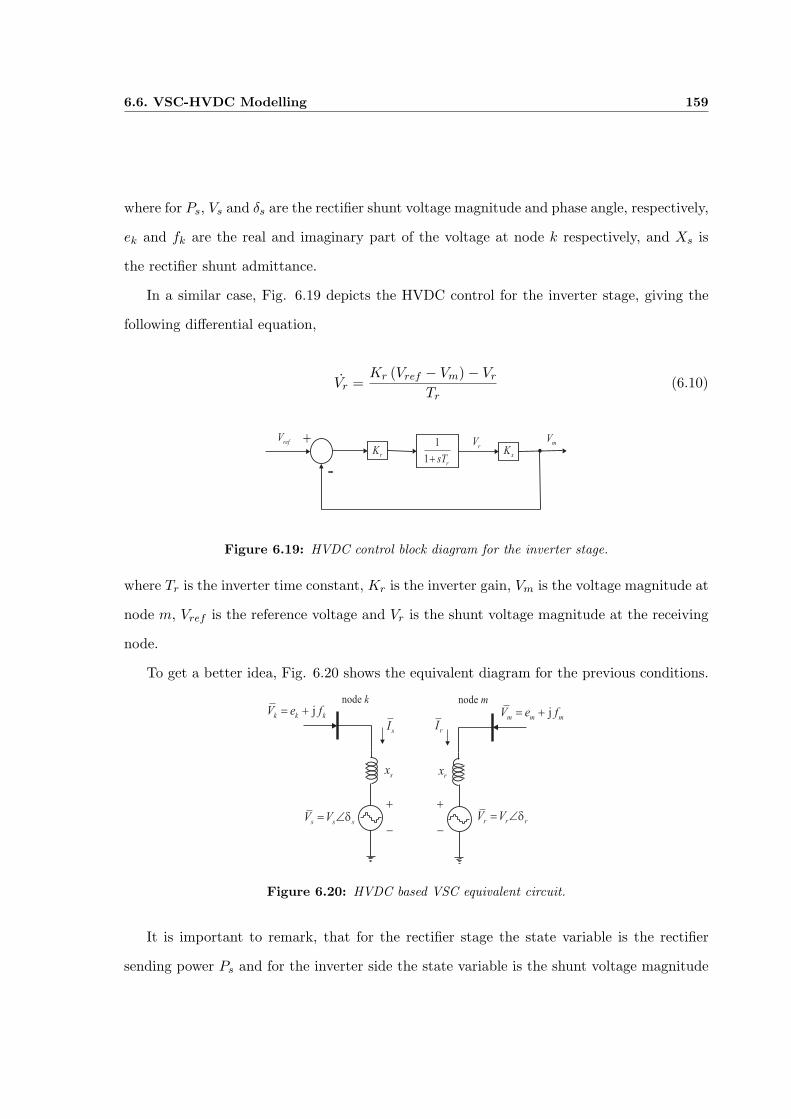
6.6. VSC-HVDC Modelling 159
where for Ps, Vs and δs are the rectifier shunt voltage magnitude and phase angle, respectively,
ek and fk are the real and imaginary part of the voltage at node k respectively, and Xs is
the rectifier shunt admittance.
In a similar case, Fig. 6.19 depicts the HVDC control for the inverter stage, giving the
following differential equation,
Vr =Kr (Vref − Vm)− Vr
Tr(6.10)
+
-
1
1r
sT+r
Km
VrefV
xK
rV
Figure 6.19: HVDC control block diagram for the inverter stage.
where Tr is the inverter time constant, Kr is the inverter gain, Vm is the voltage magnitude at
node m, Vref is the reference voltage and Vr is the shunt voltage magnitude at the receiving
node.
To get a better idea, Fig. 6.20 shows the equivalent diagram for the previous conditions.
s s sV V d= Ð
-
+
sI
jk k k
V e f= +
node m
rI
sx
-
+
r r rV V d= Ð
rx
jm m m
V e f= +
node k
Figure 6.20: HVDC based VSC equivalent circuit.
It is important to remark, that for the rectifier stage the state variable is the rectifier
sending power Ps and for the inverter side the state variable is the shunt voltage magnitude

6.7. Numerical Evaluation of Power Networks with VSC-HVDC Controller 160
Vr.
Finally Eq. 6.6 is redefined as,
FPHV DC(t) = FPs(t) − FPr(t) − FPloss(t) (6.11)
where FPS(t), FPr(t) and FPloss(t) are described as follow,
FPs(t) = −Ps
[1 +
∆t
2Ts(Ks + 1)
](6.12)
FPr(t) =FVr(t) (fm cos δr − em sin δr)
Xr(6.13)
FPloss(t) = 2(
Rdc
Vs2 Ps
)FPs(t) (6.14)
and FVr(t) is defined as,
FVr(t) = −Vr
[1 +
∆t
2Tr
]− ∆t
2TrKrVm (6.15)
In a compact way,
FPHV DC(t) =(
1− 2Rdc
Vs2 Ps
)FPs(t) − FPr(t) (6.16)
6.7 Numerical Evaluation of Power Networks with VSC-HVDC
Controller
6.7.1 Test case 4
In this section the HVDC-VSC dynamic behavior is evaluated. As in previous cases, the
nine-bus, three-machine power system depicted at Fig. 4.16, is used.
In this test case, an HVDC-VSC is replaced with the transmission line connecting Bus 5

6.7. Numerical Evaluation of Power Networks with VSC-HVDC Controller 161
and 7. It will be set to transfer 0.4 pu active power from Bus 5 to Bus 7. The rectifier is
set to regulate constant active power flow at its AC terminal, and the inverter is assumed to
exert no voltage control. The source of the perturbation is a load increment of 25% at Bus
8 at time 1 min. The simulation is carried out for 5 minutes.
Fig. 6.21 shows the voltage magnitude at all the buses, and Fig. 6.22 depicts the voltage
magnitude for the sending and receiving terminals of the HVDC. The continuous line, repre-
sents the voltage magnitude injected by the HVDC at the sending node, and the dashed line
shows the voltage magnitude injection at the receiving node.
0 0.5 1 1.5 2 2.5 3 3.5 4 4.5 50.95
0.96
0.97
0.98
0.99
1
1.01
1.02
1.03
1.04
1.05
time, min
Bus voltage magnitude, pu
Figure 6.21: Bus voltage response of the power network.
Moreover, Fig. 6.23 shows the voltage magnitude at Bus 7, having a value of around
1.015 pu. It is observed that during the transient state, the voltage magnitude injected by
the HVDC-VSC terminal, depicted in Fig. 6.22, increases in order to support the voltage
magnitude at Bus 7.
The dc-link cable is assumed to contain losses, and it has a resistance value of 0.05 pu.
The amount of transferred power is set to 0.40, as depicted in Fig. 6.24, and the power at
the receiving end of the HVDC is 0.3934 pu. The transferred power to the receiving bus is

6.7. Numerical Evaluation of Power Networks with VSC-HVDC Controller 162
0 0.5 1 1.5 2 2.5 3 3.5 4 4.5 50.94
0.95
0.96
0.97
0.98
0.99
1
1.01
1.02
time, min
Bus
volt
age
magn
itud
e, p
u
Sending node
Receiving node
Figure 6.22: Bus voltage magnitude at HVDC terminals.
0 0.5 1 1.5 2 2.5 3 3.5 4 4.5 5
1.0135
1.014
1.0145
1.015
1.0155
1.016
time, min
Bus voltage magnitude, pu
Figure 6.23: Bus voltage magnitude at Bus 7.
reduced due to the copper losses of the dc-link. It can be observed from the power result in
Fig. 6.24 that the power control in the rectifier is very effective in keeping the power at a
constant value of 0.4 pu.

6.7. Numerical Evaluation of Power Networks with VSC-HVDC Controller 163
0 0.5 1 1.5 2 2.5 3 3.5 4 4.5 50.393
0.394
0.395
0.396
0.397
0.398
0.399
0.4
0.401
0.402
time, min
HVDC
tra
nsfe
rred
pow
er,
pu
Sending node
Receiving node
Figure 6.24: HVDC-VSC transferred power when dc link losses are considered.
6.8. Summary 164
6.8 Summary
This chapter has addressed further developments on the dynamic power flow algorithm.
FACTS controllers based on voltage source converters have been developed and implemented
into the dynamic power flow algorithm. The main VSC-FACTS controllers described in this
chapter are the STATCOM and HVDC-VSC.
Several test cases have been presented. The STATCOM has been used to enhance the
voltage at a particular point of the network under both normal and abnormal operation,
such as a three-phase fault. Furthermore, this FACTS controller successfully improves the
voltage at the weakest bus of the system even when the power network is subjected to a
load perturbation. The HVDC-VSC has been set to active power transfer at the rectifier
end of the HVDC link, even in situation when a disturbance arises. The HVDC-VSC model
implemented is the dynamic power flow program has the flexibility of representing not only
point-to-point links but also back-to-back links.
Both VSC-FACTS devices enable a better performance of the whole system under un-
favourable conditions.
Chapter 7
Three-Phase Dynamic Power
Flows in abc Co-ordinates
7.1 Introduction
Worldwide, electrical power is generated, transmitted and distributed in a three-phase
fashion. Besides, the possibility of having excessive imbalances between the phase voltages or
currents in a three-phase system, has always been a concern to power engineers, due to their
detrimental effects on power system operation. In practice, typical power system contains
untransposed transmission lines and feeders, single and three-phase unbalanced static shunt
loads, single and three-phase dynamic loads such as induction motors and capacitors banks.
Generally, power systems are inherently unbalanced because of single-phase loads but also
because of the occurrence of asymmetrical spacings between line conductors [Zhang et al.,
2005].
When such transmission and load imbalances can no longer be assumed to be negligible,
positive sequence modelling and conventional power flows or power system dynamics sim-
ulations are not applicable. Instead, detailed three-phase models and solution techniques

7.2. Power System Modelling 166
must be applied if accurate assessments are to be carried out during dynamic operation of
the power system, including the most relevant power plant components such as, synchronous
generators and power loads, modelled in phase.
To carry out comprehensive dynamic analyses of unbalanced transmission systems, it is
mandatory to have a three-phase dynamic power flow algorithm in abc co-ordinates. Likewise
its positive sequence counterpart presented in Chapter 4, for the solution of three-phase
balanced power systems, the three-phase dynamic power flows can be modelled as a set of
non-linear algebraic and differential equations representing the power network, rotating power
machinery and controls.
The different static and dynamic elements that comprise the electric power system are
modelled in the abc frame of reference to develop the three-phase dynamic power flow algo-
rithm in rectangular co-ordinates.
All the relevant power system elements for dynamic power flows analyses, have been
described in foregoing chapters; however the dynamic power flow modelling carried out has
been positive sequence analyses. Thus, the modelling needs to be extended, in such a way
that it is amenable to dynamic power flows studies in abc co-ordinates.
7.2 Power System Modelling
7.2.1 Three-phase synchronous machine modelling
The classical theory of synchronous machines for dq co-ordinates is well defined [Kimbark,
1948b,Concordia, 1951]. In this thesis, the mathematical theory presented is based on the
full dq0 co-ordinate system [Park, 1929].
The phase voltages and currents at the terminal of the synchronous generators are, re-
spectively:
7.2. Power System Modelling 167
Va = Vt1sin(θ1)
Vb = Vt2sin(θ2 − 120)
Vc = Vt3sin(θ3 + 120)
(7.1)
and
Ia = It1sin(ψ1)
Ib = It2sin(ψ2 − 120)
Ic = It3sin(ψ3 + 120)
(7.2)
where
Vt is the bus voltage magnitude at bus terminals.
It is the bus voltage magnitude at bus terminals.
θ is defined as the voltage angle.
ψ is defined as the current angle.
Fig. 7.1 schematically describes a three-phase synchronous generator from a circuit theory
point of view.
The matrix transformation used to transform the abc phase variables into dq0 variables
is the following one [Park, 1929]:
[Tdq0] =23
cos θ cos(θ − 2π
3
)cos
(θ + 2π
3
)
sin θ sin(θ − 2π
3
)sin
(θ + 2π
3
)
12
12
12
(7.3)
In generic form, including voltages and currents, the transformation operations used for
referring the stator quantities to the rotor side and viceversa are:
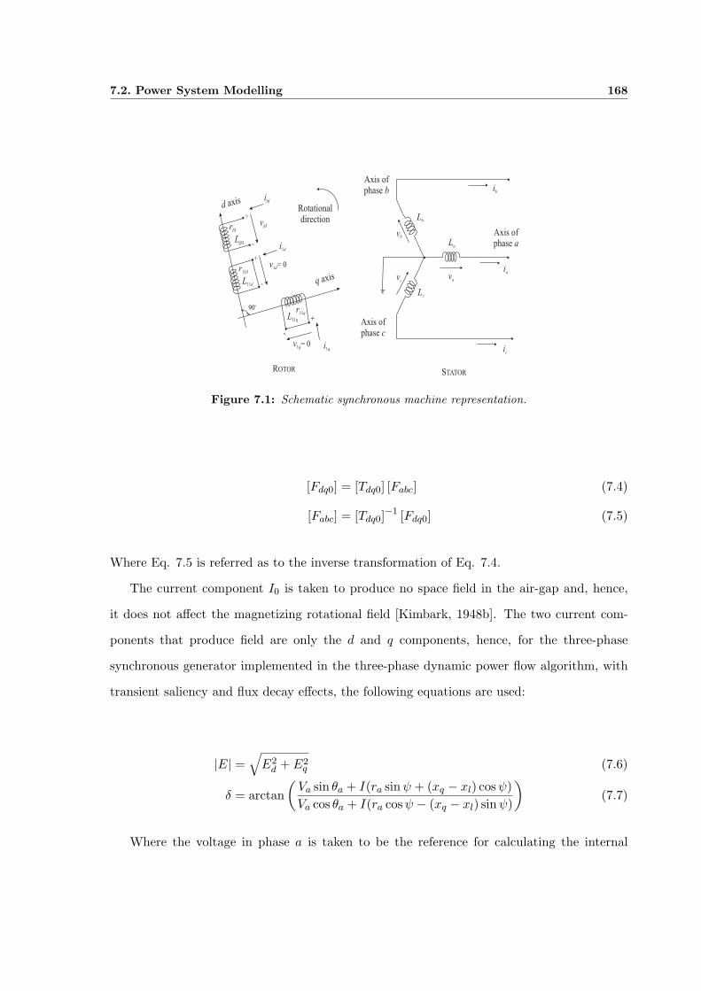
7.2. Power System Modelling 168
vb
ib
Lb
Axis of
phase a
STATOR
Axis of
phase c
Axis of
phase b
ic
vav
c
La
Lc
ia
+
-
v1d
= 0
i1d
L11d
r11d
+
-
vfd
ifd
Lffd
rfd
90o
-
v1q
= 0 i1q
r11q
+L11q
d axis
q axis
ROTOR
Rotational
direction
Figure 7.1: Schematic synchronous machine representation.
[Fdq0] = [Tdq0] [Fabc] (7.4)
[Fabc] = [Tdq0]−1 [Fdq0] (7.5)
Where Eq. 7.5 is referred as to the inverse transformation of Eq. 7.4.
The current component I0 is taken to produce no space field in the air-gap and, hence,
it does not affect the magnetizing rotational field [Kimbark, 1948b]. The two current com-
ponents that produce field are only the d and q components, hence, for the three-phase
synchronous generator implemented in the three-phase dynamic power flow algorithm, with
transient saliency and flux decay effects, the following equations are used:
|E| =√
E2d + E2
q (7.6)
δ = arctan(
Va sin θa + I(ra sinψ + (xq − xl) cos ψ)Va cos θa + I(ra cosψ − (xq − xl) sin ψ)
)(7.7)
Where the voltage in phase a is taken to be the reference for calculating the internal
7.2. Power System Modelling 169
voltage angle [Kundur, 1994].
7.2.2 Dynamic three-phase load tap changer model
Three-phase banks of transformers are made up of three single-phase transformers, where
the most common winding connections are: star-star, delta-delta and star-delta.
For star-star and delta-delta connected transformers, the relationship between the base
voltages and the nominal turns of the primary and secondary sides of the transformer keeps
equal for each phase [Kundur, 1994]. Nonetheless, for the star-delta transformer connection,
there is a factor of√
3 involved because of the winding connection. Likewise, a 30◦ phase
shift must be considered between the line-to-line and line-to-neutral voltages.
The dynamic element of the three-phase load tap changer is described by the following
differential equation,
Tk =1
HT
(√(eρk
)2 +(fρ
k
)2 − V0
)(7.8)
where HT is the tap’s servomotor inertia, ek and fk are the real and imaginary parts of the
voltage at the regulated bus, V0 is the target voltage magnitude and ρ is used to denote
phases a, b and c.
The dynamic three-phase load tap changer is discrete, and varies over time as a function
of nodal voltages eρk and fρ
k and the tap step size ∆Tk. Moreover, its pre-defined operating
range provide hard limits which can not be violated.
The differential equation that describes the dynamic behaviour of the three-phase load
tap changer is transformed into an algebraic equation and appended to the existing set of
algebraic equations for a unified solution. Thus, Eq. 7.8 is discretised as follows.

7.2. Power System Modelling 170
FTk(t) − FTk(t−∆t) = Tk(t) +∆t
2Ht
√(eρk(t)
)2+
(fρ
k(t)
)2− V0
+ Tk(t−∆t) +∆t
2Ht
√(eρk(t−∆t)
)2+
(fρ
k(t−∆t)
)2− V0
(7.9)
in compact form, it can be re-written as follows,
FTk= FTk(t) + FTk(t−∆t) + CTk
= 0 (7.10)
where
FTk(t) = Tk(t) −∆t
2Ht
√(eρk(t)
)2+
(fρ
k(t)
)2
FTk(t−∆t) = −Tk(t−∆t) −∆t
2Ht
√(eρk(t−∆t)
)2+
(fρ
k(t−∆t)
)2
CTk=
∆tV0
Ht
It is important to mention that a single tap parameter Tk is used for the three-phases in
the three-phase primary winding.
V0
+
-1
TH
1
s
Vk
n
-
+
kT
kTD
Tap step
size
maxkT
kT& 1k
T
minkT
Current Tap
position
Figure 7.2: Dynamic load tap changer model.
The dynamic load tap changer model is depicted at Fig. 7.2, and Fig. 7.3 shows the
discrete tap representation for each phase.
The three-phase connection for a solidly grounded star-star winding transformer is de-
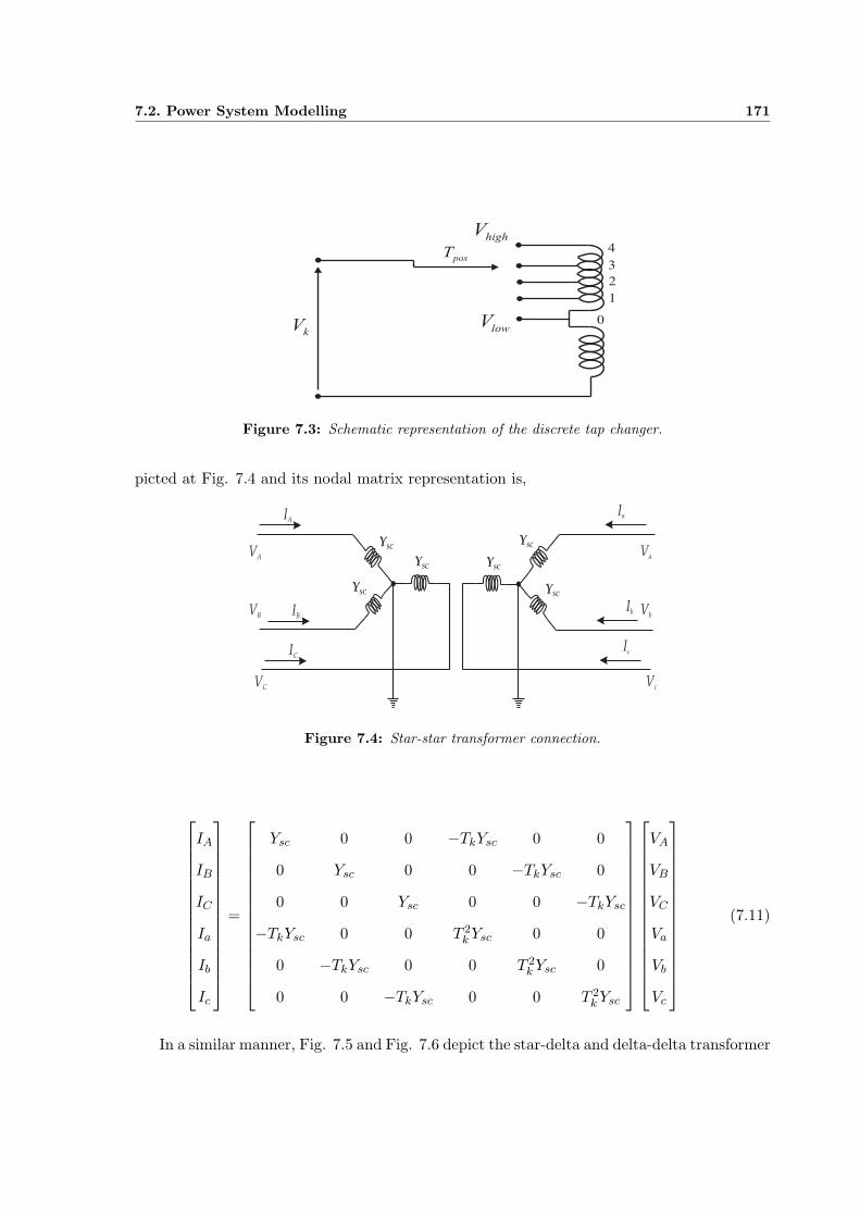
7.2. Power System Modelling 171
kV low
V
highV
posT
0
2
3
4
1
Figure 7.3: Schematic representation of the discrete tap changer.
picted at Fig. 7.4 and its nodal matrix representation is,
IA
VA
YSC
YSC
YSC
VB
VC
IB
IC
Va
Vb
Vc
Ia
Ib
Ic
YSC
YSC
YSC
Figure 7.4: Star-star transformer connection.
IA
IB
IC
Ia
Ib
Ic
=
Ysc 0 0 −TkYsc 0 0
0 Ysc 0 0 −TkYsc 0
0 0 Ysc 0 0 −TkYsc
−TkYsc 0 0 T 2k Ysc 0 0
0 −TkYsc 0 0 T 2k Ysc 0
0 0 −TkYsc 0 0 T 2k Ysc
VA
VB
VC
Va
Vb
Vc
(7.11)
In a similar manner, Fig. 7.5 and Fig. 7.6 depict the star-delta and delta-delta transformer

7.2. Power System Modelling 172
connection, respectively.
IA
VA
YSC
YSC
YSC
VB
VC
IB
IC
Va
Vc
Vb
Ia
Ic
Ib
YSC Y
SC
YSC
Figure 7.5: Star-delta transformer connection.
Va
Vc
Vb
Ia
Ic
Ib
YSC
YSC
YSCY
SC
YSC
YSC
IA
IB
IC
VA
VB
VC
Figure 7.6: Delta-delta transformer connection.
The corresponding nodal matrices for this connections are respectively,
IA
IB
IC
Ia
Ib
Ic
=13
2Ysc −Ysc −Ysc −2TkYsc TkYsc TkYsc
−Ysc 2Ysc Ysc −TkYsc −2TkYsc TkYsc
−Ysc −Ysc 2Ysc TkYsc TkYsc −2TkYsc
−2TkYsc TkYsc TkYsc 2T 2k Ysc −T 2
k Ysc T 2k Ysc
TkYsc −2TkYsc TkYsc −T 2k Ysc 2T 2
k Ysc −T 2k Ysc
TkYsc TkYsc −2TkYsc −T 2k Ysc −T 2
k Ysc 2T 2k Ysc
VA
VB
VC
Va
Vb
Vc
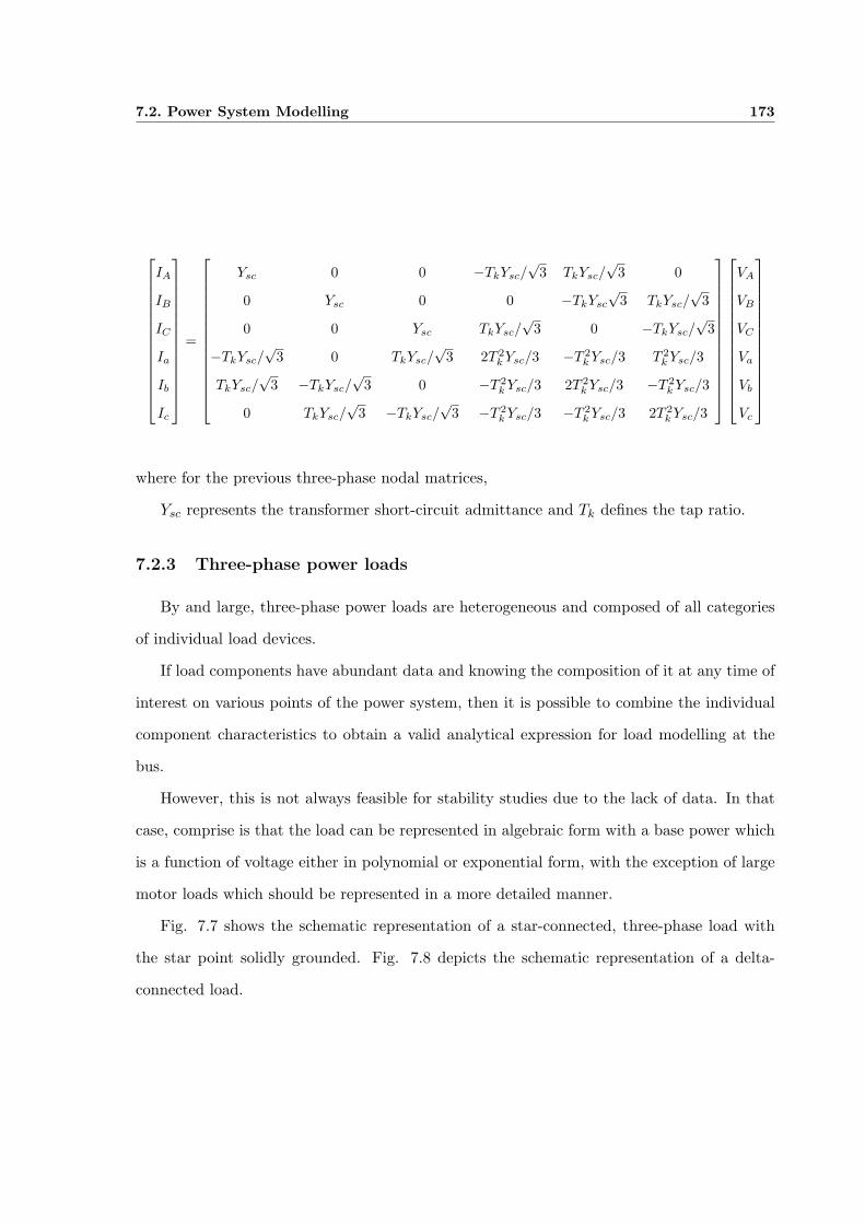
7.2. Power System Modelling 173
IA
IB
IC
Ia
Ib
Ic
=
Ysc 0 0 −TkYsc/√
3 TkYsc/√
3 0
0 Ysc 0 0 −TkYsc
√3 TkYsc/
√3
0 0 Ysc TkYsc/√
3 0 −TkYsc/√
3
−TkYsc/√
3 0 TkYsc/√
3 2T 2k Ysc/3 −T 2
k Ysc/3 T 2k Ysc/3
TkYsc/√
3 −TkYsc/√
3 0 −T 2k Ysc/3 2T 2
k Ysc/3 −T 2k Ysc/3
0 TkYsc/√
3 −TkYsc/√
3 −T 2k Ysc/3 −T 2
k Ysc/3 2T 2k Ysc/3
VA
VB
VC
Va
Vb
Vc
where for the previous three-phase nodal matrices,
Ysc represents the transformer short-circuit admittance and Tk defines the tap ratio.
7.2.3 Three-phase power loads
By and large, three-phase power loads are heterogeneous and composed of all categories
of individual load devices.
If load components have abundant data and knowing the composition of it at any time of
interest on various points of the power system, then it is possible to combine the individual
component characteristics to obtain a valid analytical expression for load modelling at the
bus.
However, this is not always feasible for stability studies due to the lack of data. In that
case, comprise is that the load can be represented in algebraic form with a base power which
is a function of voltage either in polynomial or exponential form, with the exception of large
motor loads which should be represented in a more detailed manner.
Fig. 7.7 shows the schematic representation of a star-connected, three-phase load with
the star point solidly grounded. Fig. 7.8 depicts the schematic representation of a delta-
connected load.
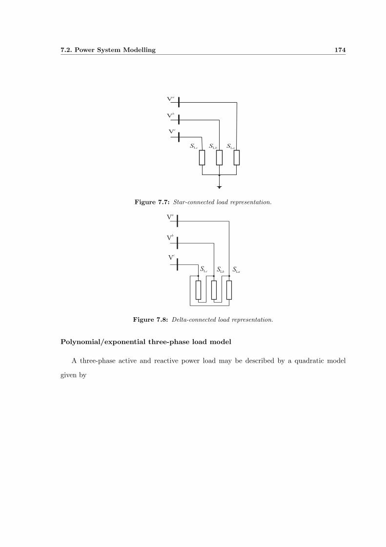
7.2. Power System Modelling 174
Vc
SLb
SLc
SLa
Vb
Va
Figure 7.7: Star-connected load representation.
Vc
SLb
SLc S
La
Vb
Va
Figure 7.8: Delta-connected load representation.
Polynomial/exponential three-phase load model
A three-phase active and reactive power load may be described by a quadratic model
given by
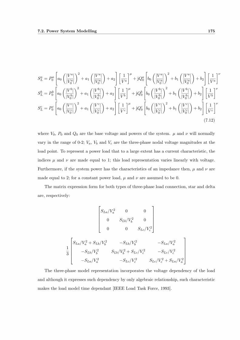
7.2. Power System Modelling 175
SaL = P a
0
[a0
( |V a||V a
0 |)2
+ a1
( |V a||V a
0 |)
+ a2
][1
V a
]µ
+ jQa0
[b0
( |V a||V a
0 |)2
+ b1
( |V a||V a
0 |)
+ b2
][1
V a
]ν
SbL = P b
0
[a0
( |V b||V b
0 |
)2
+ a1
( |V b||V b
0 |
)+ a2
][1
V b
]µ
+ jQb0
[b0
( |V b||V b
0 |
)2
+ b1
( |V b||V b
0 |
)+ b2
][1
V b
]ν
ScL = P c
0
[a0
( |V c||V c
0 |)2
+ a1
( |V c||V c
0 |)
+ a2
][1
V c
]µ
+ jQc0
[b0
( |V c||V c
0 |)2
+ b1
( |V c||V c
0 |)
+ b2
][1
V c
]ν
(7.12)
where V0, P0 and Q0 are the base voltage and powers of the system. µ and ν will normally
vary in the range of 0-2; Va, Vb and Vc are the three-phase nodal voltage magnitudes at the
load point. To represent a power load that to a large extent has a current characteristic, the
indices µ and ν are made equal to 1; this load representation varies linearly with voltage.
Furthermore, if the system power has the characteristics of an impedance then, µ and ν are
made equal to 2; for a constant power load, µ and ν are assumed to be 0.
The matrix expression form for both types of three-phase load connection, star and delta
are, respectively:
SLa/V 2a 0 0
0 SLb/V 2b 0
0 0 SLc/V 2c
13
SLa/V 2a + SLb/V 2
b −SLb/V 2b −SLa/V 2
a
−SLb/V 2b SLb/V 2
b + SLc/V 2c −SLc/V 2
c
−SLa/V 2a −SLc/V 2
c SLc/V 2c + SLa/V 2
a
The three-phase model representation incorporates the voltage dependency of the load
and although it expresses such dependency by only algebraic relationship, such characteristic
makes the load model time dependant [IEEE Load Task Force, 1993].
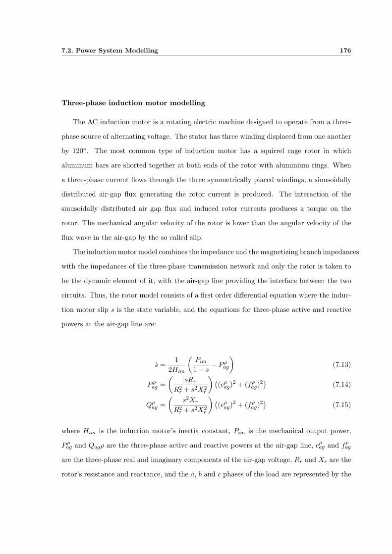
7.2. Power System Modelling 176
Three-phase induction motor modelling
The AC induction motor is a rotating electric machine designed to operate from a three-
phase source of alternating voltage. The stator has three winding displaced from one another
by 120◦. The most common type of induction motor has a squirrel cage rotor in which
aluminum bars are shorted together at both ends of the rotor with aluminium rings. When
a three-phase current flows through the three symmetrically placed windings, a sinusoidally
distributed air-gap flux generating the rotor current is produced. The interaction of the
sinusoidally distributed air gap flux and induced rotor currents produces a torque on the
rotor. The mechanical angular velocity of the rotor is lower than the angular velocity of the
flux wave in the air-gap by the so called slip.
The induction motor model combines the impedance and the magnetizing branch impedances
with the impedances of the three-phase transmission network and only the rotor is taken to
be the dynamic element of it, with the air-gap line providing the interface between the two
circuits. Thus, the rotor model consists of a first order differential equation where the induc-
tion motor slip s is the state variable, and the equations for three-phase active and reactive
powers at the air-gap line are:
s =1
2Him
(Pim
1− s− P ρ
ag
)(7.13)
P ρag =
(sRr
R2r + s2X2
r
) ((eρ
ag)2 + (fρ
ag)2)
(7.14)
Qρag =
(s2Xr
R2r + s2X2
r
) ((eρ
ag)2 + (fρ
ag)2)
(7.15)
where Him is the induction motor’s inertia constant, Pim is the mechanical output power,
P ρag and Qagρ are the three-phase active and reactive powers at the air-gap line, eρ
ag and fρag
are the three-phase real and imaginary components of the air-gap voltage, Rr and Xr are the
rotor’s resistance and reactance, and the a, b and c phases of the load are represented by the
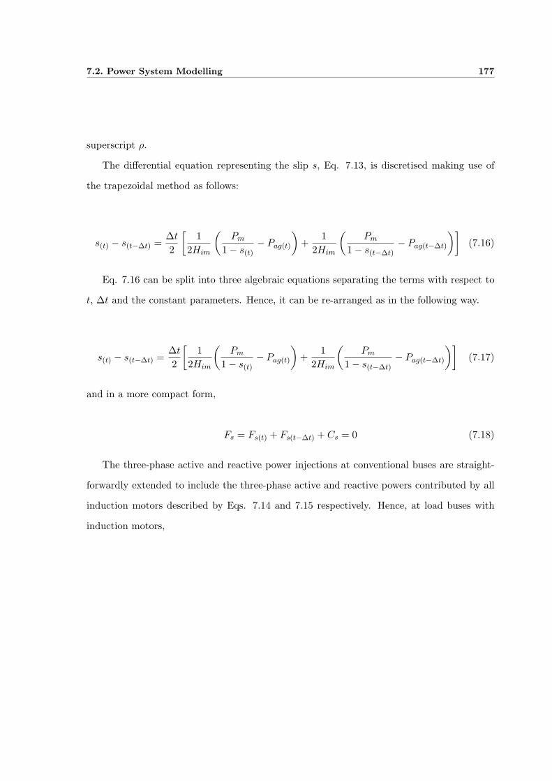
7.2. Power System Modelling 177
superscript ρ.
The differential equation representing the slip s, Eq. 7.13, is discretised making use of
the trapezoidal method as follows:
s(t) − s(t−∆t) =∆t
2
[1
2Him
(Pm
1− s(t)− Pag(t)
)+
12Him
(Pm
1− s(t−∆t)− Pag(t−∆t)
)](7.16)
Eq. 7.16 can be split into three algebraic equations separating the terms with respect to
t, ∆t and the constant parameters. Hence, it can be re-arranged as in the following way.
s(t) − s(t−∆t) =∆t
2
[1
2Him
(Pm
1− s(t)− Pag(t)
)+
12Him
(Pm
1− s(t−∆t)− Pag(t−∆t)
)](7.17)
and in a more compact form,
Fs = Fs(t) + Fs(t−∆t) + Cs = 0 (7.18)
The three-phase active and reactive power injections at conventional buses are straight-
forwardly extended to include the three-phase active and reactive powers contributed by all
induction motors described by Eqs. 7.14 and 7.15 respectively. Hence, at load buses with
induction motors,

7.3. Dynamic Simulations of Three-Phase Power Networks 178
P a(m) + P a
ag(imbus(n))
P b(m) + P b
ag(imbus(n))
P c(m) + P c
ag(imbus(n))
Qa(m) + Qa
ag(imbus(n))
Qb(m) + Qb
ag(imbus(n))
Qc(m) + Qc
ag(imbus(n))
(7.19)
for m=1,. . .,nbus and n=1,. . .,nim, where imbus(n) is an array of induction motor-connected
buses.
7.3 Dynamic Simulations of Three-Phase Power Networks
7.3.1 Test case 1
The nine-bus, three-machine power system depicted by the one-line schematic diagram
of Fig. 4.16, is adopted and extended to carry out three-phase dynamic power flows studies.
An unbalanced load perturbation is carried out. At minute 1 the load connected at Bus 6 is
reduced by 30, 25 and 20% of its initial value for phase a, b and c respectively. Later on at
minute 3, the load connected at Bus 8 is increased by 45, 50 and 55% of its original value
for phases a, b and c respectively. The simulation is run for ten minutes. The three-phase
power loads are represented by their static load model and the unbalanced values are given
at Table 7.1.
Fig. 7.10 shows the three-phase bus voltage magnitude for balanced load reduction of
25% at time 1 min and balanced load increment of 50% at minute 3. Fig. 7.9 depicts the
condition where unbalanced load conditions are carried out. For the balanced load condition,
the perturbation carried out is the same as for phase b of the unbalanced case. It is taken as
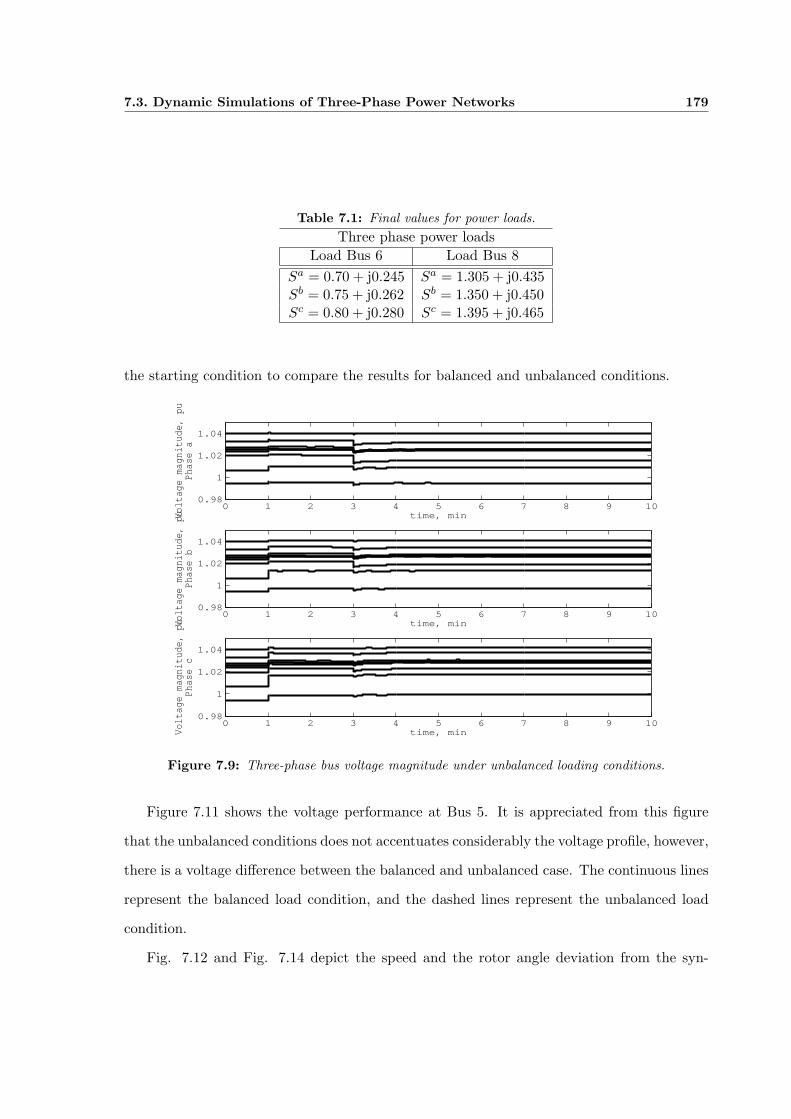
7.3. Dynamic Simulations of Three-Phase Power Networks 179
Table 7.1: Final values for power loads.Three phase power loads
Load Bus 6 Load Bus 8Sa = 0.70 + j0.245 Sa = 1.305 + j0.435Sb = 0.75 + j0.262 Sb = 1.350 + j0.450Sc = 0.80 + j0.280 Sc = 1.395 + j0.465
the starting condition to compare the results for balanced and unbalanced conditions.
0 1 2 3 4 5 6 7 8 9 100.98
1
1.02
1.04
time, minVoltage magnitude, pu
Phase a
0 1 2 3 4 5 6 7 8 9 100.98
1
1.02
1.04
time, minVoltage magnitude, pu
Phase b
0 1 2 3 4 5 6 7 8 9 100.98
1
1.02
1.04
time, minVoltage magnitude, pu
Phase c
Figure 7.9: Three-phase bus voltage magnitude under unbalanced loading conditions.
Figure 7.11 shows the voltage performance at Bus 5. It is appreciated from this figure
that the unbalanced conditions does not accentuates considerably the voltage profile, however,
there is a voltage difference between the balanced and unbalanced case. The continuous lines
represent the balanced load condition, and the dashed lines represent the unbalanced load
condition.
Fig. 7.12 and Fig. 7.14 depict the speed and the rotor angle deviation from the syn-
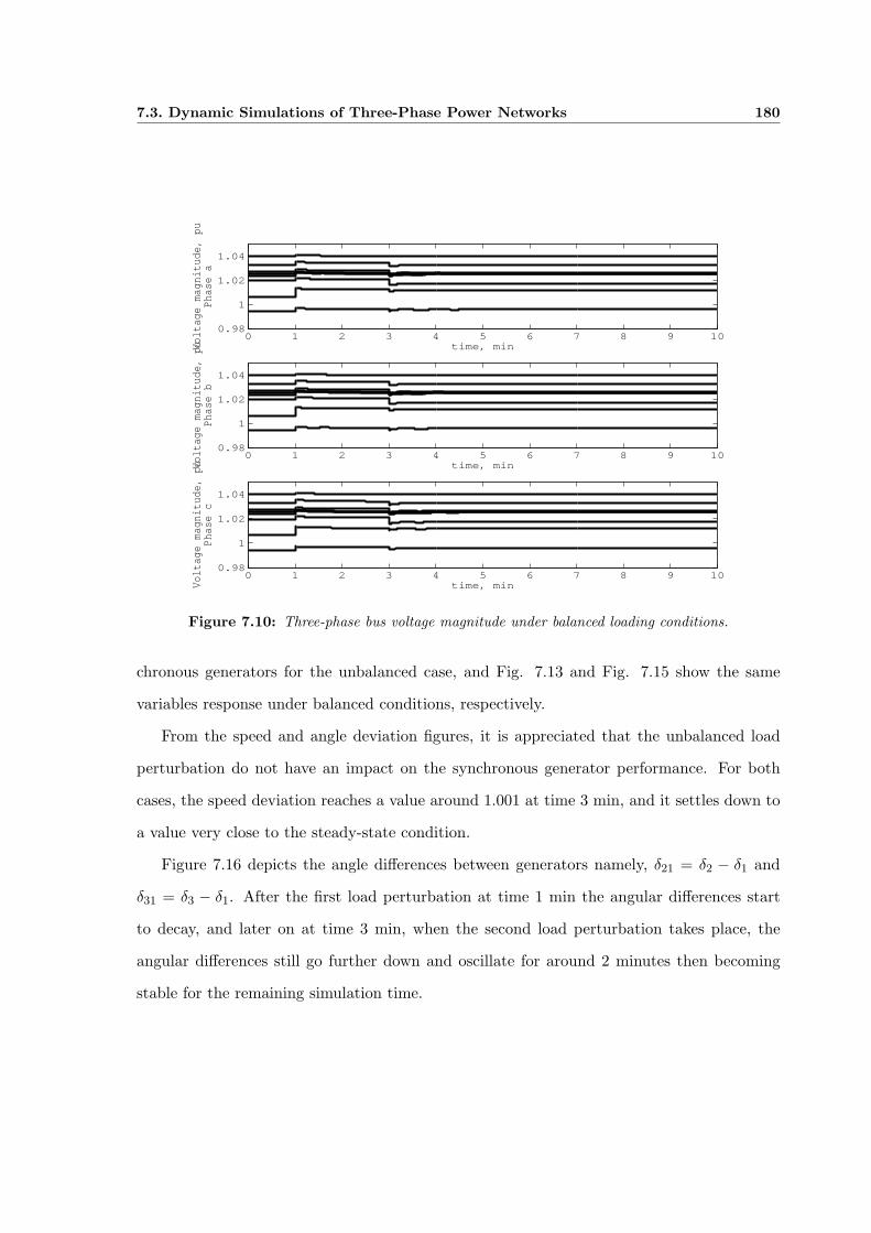
7.3. Dynamic Simulations of Three-Phase Power Networks 180
0 1 2 3 4 5 6 7 8 9 100.98
1
1.02
1.04
time, minVoltage magnitude, pu
Phase a
0 1 2 3 4 5 6 7 8 9 100.98
1
1.02
1.04
time, minVoltage magnitude, pu
Phase b
0 1 2 3 4 5 6 7 8 9 100.98
1
1.02
1.04
time, minVoltage magnitude, pu
Phase c
Figure 7.10: Three-phase bus voltage magnitude under balanced loading conditions.
chronous generators for the unbalanced case, and Fig. 7.13 and Fig. 7.15 show the same
variables response under balanced conditions, respectively.
From the speed and angle deviation figures, it is appreciated that the unbalanced load
perturbation do not have an impact on the synchronous generator performance. For both
cases, the speed deviation reaches a value around 1.001 at time 3 min, and it settles down to
a value very close to the steady-state condition.
Figure 7.16 depicts the angle differences between generators namely, δ21 = δ2 − δ1 and
δ31 = δ3 − δ1. After the first load perturbation at time 1 min the angular differences start
to decay, and later on at time 3 min, when the second load perturbation takes place, the
angular differences still go further down and oscillate for around 2 minutes then becoming
stable for the remaining simulation time.

7.3. Dynamic Simulations of Three-Phase Power Networks 181
0 1 2 3 4 5 6 7 8 9 100.99
0.995
1
time, min
Phase a
0 1 2 3 4 5 6 7 8 9 100.99
0.992
0.994
0.996
0.998
1
time, min
Voltage magnitude at Bus 5, pu
Phase b
0 1 2 3 4 5 6 7 8 9 100.99
0.995
1
1.005
time, min
Phase c
Figure 7.11: Three-phase voltage magnitude at Bus 5 under balanced and unbalanced loading condi-tions.
0 1 2 3 4 5 6 7 8 9 101
1.0002
1.0004
1.0006
1.0008
1.001
1.0012
time, min
Speed deviation
ω 1, pu
ω1
ω2
ω3
Figure 7.12: Synchronous generators speed deviation under unbalanced loading conditions.
7.3.2 Test case 2
To show the flexibility of the three-phase dynamic power flows algorithm, a series fault
involving one phase of a transmission line opening is carried out. As in the previous test

7.3. Dynamic Simulations of Three-Phase Power Networks 182
0 1 2 3 4 5 6 7 8 9 101
1.0002
1.0004
1.0006
1.0008
1.001
1.0012
time, min
Speed deviation
ω 1, pu
ω1
ω2
ω3
Figure 7.13: Synchronous generators speed deviation under balanced loading conditions.
0 1 2 3 4 5 6 7 8 9 100
0.2
0.4
0.6
0.8
1
1.2
1.4
time, min
Roto
r an
gle
devi
atio
n δ i,
degr
ees
δ1
δ2
δ3
Figure 7.14: Rotor angle deviation under unbalanced loading conditions.
case, the three-machine nine-bus power system is used to carry out the study. The phase
a of the transmission line which connects buses 5 and 7 is disconnected at time 1 min; as
a consequence of this action the bus voltage magnitude of phase a of the system is reduced
considerably compared to the voltages in phases b and c. Fig. 7.17 depicts the bus voltage
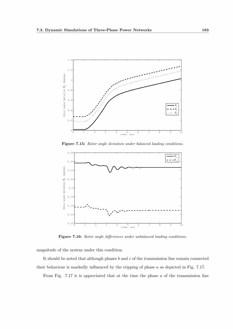
7.3. Dynamic Simulations of Three-Phase Power Networks 183
0 1 2 3 4 5 6 7 8 9 100
0.2
0.4
0.6
0.8
1
1.2
1.4
time, min
Roto
r an
gle
devi
atio
n δ i,
degr
ees
δ1
δ2
δ3
Figure 7.15: Rotor angle deviation under balanced loading conditions.
0 1 2 3 4 5 6 7 8 9 100.12
0.14
0.16
0.18
0.2
0.22
0.24
0.26
0.28
time, min
Roto
r an
gle
devi
atio
n δ i,
degr
ees
δ21
δ31
Figure 7.16: Rotor angle differences under unbalanced loading conditions.
magnitude of the system under this condition.
It should be noted that although phases b and c of the transmission line remain connected
their behaviour is markedly influenced by the tripping of phase a as depicted in Fig. 7.17.
From Fig. 7.17 it is appreciated that at the time the phase a of the transmission line
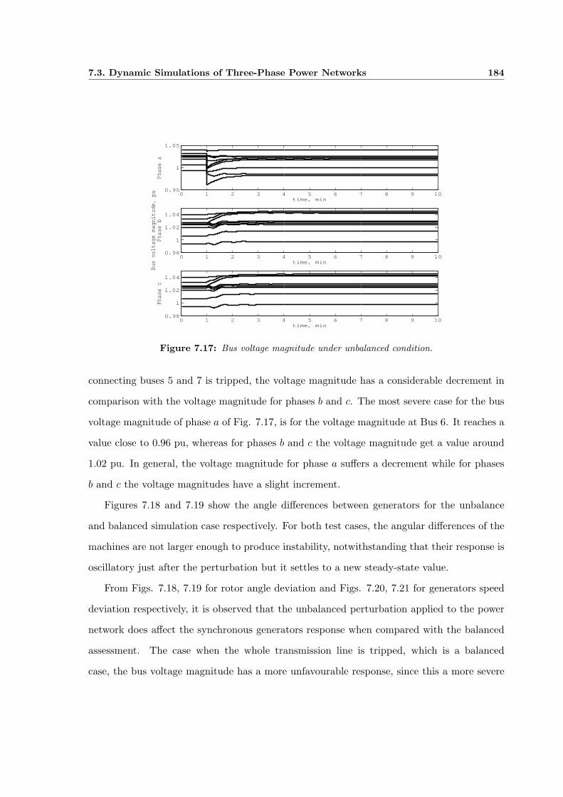
7.3. Dynamic Simulations of Three-Phase Power Networks 184
0 1 2 3 4 5 6 7 8 9 100.95
1
1.05
time, min
Phase a
0 1 2 3 4 5 6 7 8 9 100.98
1
1.02
1.04
time, min
Bus voltage magnitude, pu
Phase b
0 1 2 3 4 5 6 7 8 9 100.98
1
1.02
1.04
time, min
Phase c
Figure 7.17: Bus voltage magnitude under unbalanced condition.
connecting buses 5 and 7 is tripped, the voltage magnitude has a considerable decrement in
comparison with the voltage magnitude for phases b and c. The most severe case for the bus
voltage magnitude of phase a of Fig. 7.17, is for the voltage magnitude at Bus 6. It reaches a
value close to 0.96 pu, whereas for phases b and c the voltage magnitude get a value around
1.02 pu. In general, the voltage magnitude for phase a suffers a decrement while for phases
b and c the voltage magnitudes have a slight increment.
Figures 7.18 and 7.19 show the angle differences between generators for the unbalance
and balanced simulation case respectively. For both test cases, the angular differences of the
machines are not larger enough to produce instability, notwithstanding that their response is
oscillatory just after the perturbation but it settles to a new steady-state value.
From Figs. 7.18, 7.19 for rotor angle deviation and Figs. 7.20, 7.21 for generators speed
deviation respectively, it is observed that the unbalanced perturbation applied to the power
network does affect the synchronous generators response when compared with the balanced
assessment. The case when the whole transmission line is tripped, which is a balanced
case, the bus voltage magnitude has a more unfavourable response, since this a more severe

7.3. Dynamic Simulations of Three-Phase Power Networks 185
0 1 2 3 4 5 6 7 8 9 100.05
0.1
0.15
0.2
0.25
0.3
time, min
Ang
le d
iffer
ence
s, ra
dδ
2 − δ
1
δ3 − δ
1
Figure 7.18: Angle differences under unbalanced condition.
0 1 2 3 4 5 6 7 8 9 10−0.2
−0.1
0
0.1
0.2
0.3
0.4
0.5
0.6
time, min
Ang
le d
iffer
ence
s, ra
d
δ2 − δ
1
δ3 − δ
1
Figure 7.19: Angle differences under balanced condition.
perturbation than just the tripping of one phase of the transmission line. Fig. 7.22 shows
the bus voltage magnitude for the tripping of the whole transmission line.
It is observed in Figs. 7.20 and 7.21 that the maximum speed deviation is 1.001 pu at
time 3 min and then it drops sharply to a value of around 1.00017 pu.
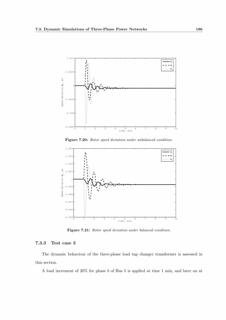
7.3. Dynamic Simulations of Three-Phase Power Networks 186
0 1 2 3 4 5 6 7 8 9 100.9985
0.999
0.9995
1
1.0005
1.001
time, min
Spee
d de
viat
ion
ω 1,
puω1
ω2
ω3
Figure 7.20: Rotor speed deviation under unbalanced condition.
0 1 2 3 4 5 6 7 8 9 100.995
0.996
0.997
0.998
0.999
1
1.001
1.002
1.003
1.004
time, min
Spee
d de
viat
ion
ω 1,
pu
ω1
ω2
ω3
Figure 7.21: Rotor speed deviation under balanced condition.
7.3.3 Test case 3
The dynamic behaviour of the three-phase load tap changer transformer is assessed in
this section.
A load increment of 20% for phase b of Bus 5 is applied at time 1 min, and later on at
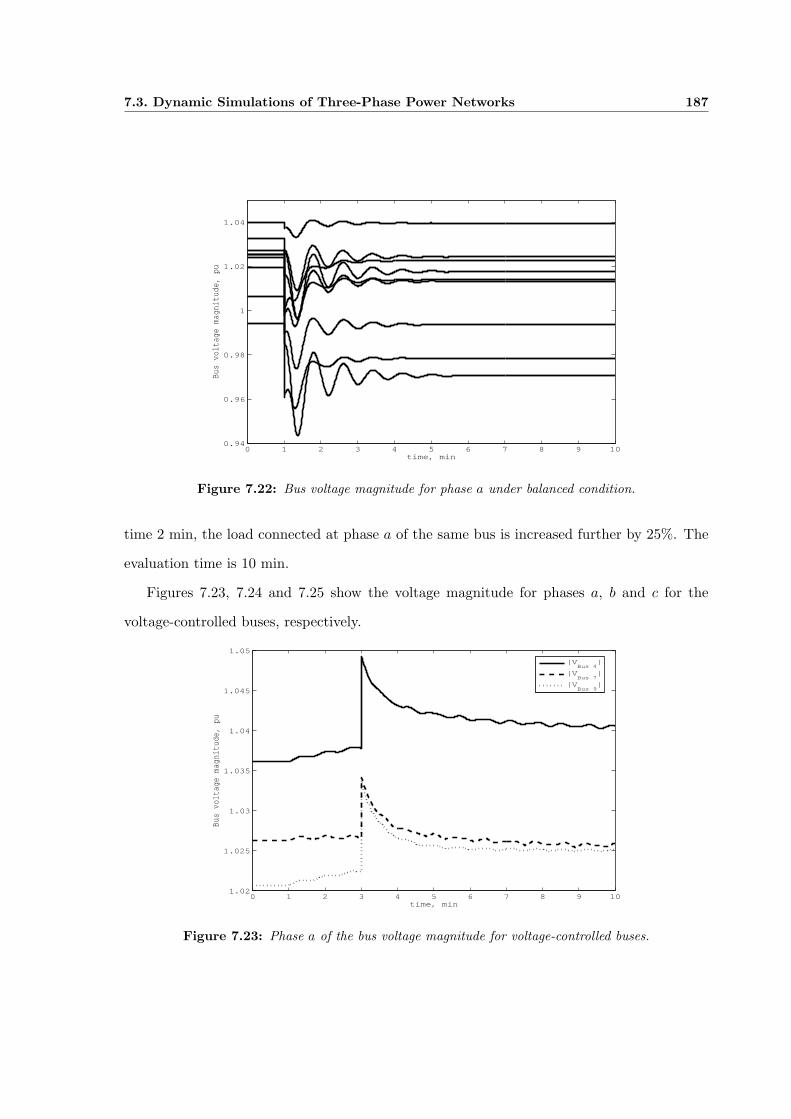
7.3. Dynamic Simulations of Three-Phase Power Networks 187
0 1 2 3 4 5 6 7 8 9 100.94
0.96
0.98
1
1.02
1.04
time, min
Bus voltage magnitude, pu
Figure 7.22: Bus voltage magnitude for phase a under balanced condition.
time 2 min, the load connected at phase a of the same bus is increased further by 25%. The
evaluation time is 10 min.
Figures 7.23, 7.24 and 7.25 show the voltage magnitude for phases a, b and c for the
voltage-controlled buses, respectively.
0 1 2 3 4 5 6 7 8 9 101.02
1.025
1.03
1.035
1.04
1.045
1.05
time, min
Bus
volt
age
magn
itud
e, p
u
|VBus 4
|
|VBus 7
|
|VBus 9
|
Figure 7.23: Phase a of the bus voltage magnitude for voltage-controlled buses.
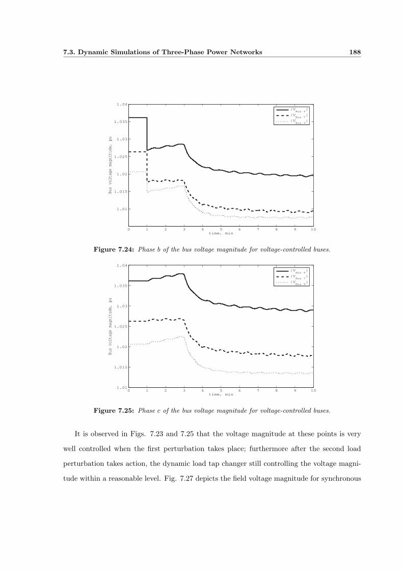
7.3. Dynamic Simulations of Three-Phase Power Networks 188
0 1 2 3 4 5 6 7 8 9 10
1.01
1.015
1.02
1.025
1.03
1.035
1.04
time, min
Bus voltage magnitude, pu
|VBus 4
|
|VBus 7
|
|VBus 9
|
Figure 7.24: Phase b of the bus voltage magnitude for voltage-controlled buses.
0 1 2 3 4 5 6 7 8 9 101.01
1.015
1.02
1.025
1.03
1.035
1.04
time, min
Bus voltage magnitude, pu
|VBus 4
|
|VBus 7
|
|VBus 9
|
Figure 7.25: Phase c of the bus voltage magnitude for voltage-controlled buses.
It is observed in Figs. 7.23 and 7.25 that the voltage magnitude at these points is very
well controlled when the first perturbation takes place; furthermore after the second load
perturbation takes action, the dynamic load tap changer still controlling the voltage magni-
tude within a reasonable level. Fig. 7.27 depicts the field voltage magnitude for synchronous
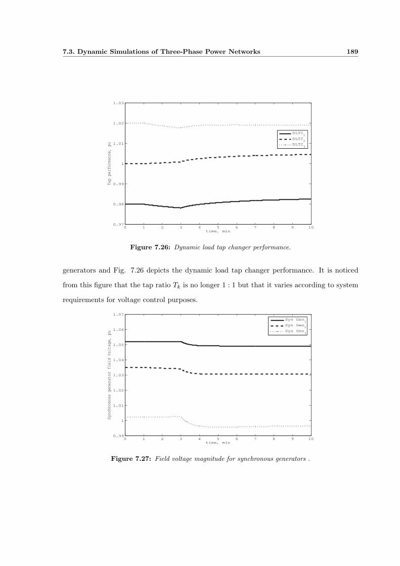
7.3. Dynamic Simulations of Three-Phase Power Networks 189
0 1 2 3 4 5 6 7 8 9 100.97
0.98
0.99
1
1.01
1.02
1.03
time, min
Tap
perf
orma
nce,
pu
DLTC1
DLTC2
DLTC3
Figure 7.26: Dynamic load tap changer performance.
generators and Fig. 7.26 depicts the dynamic load tap changer performance. It is noticed
from this figure that the tap ratio Tk is no longer 1 : 1 but that it varies according to system
requirements for voltage control purposes.
0 1 2 3 4 5 6 7 8 9 100.99
1
1.01
1.02
1.03
1.04
1.05
1.06
1.07
time, min
Sync
hron
ous
gene
rato
r fi
eld
volt
age,
pu
Syn Gen1
Syn Gen2
Syn Gen3
Figure 7.27: Field voltage magnitude for synchronous generators .

7.3. Dynamic Simulations of Three-Phase Power Networks 190
7.3.4 Test case 4
At this section the three-phase induction motor behaviour is analysed. The same power
network used in the last test case is applied to carry out this assessment.
To demonstrate the applicability and versatility of the dynamic power flows tool and the
induction motor modelling, the loads of buses 5 and 6 of Fig. 4.16 have been replaced for
two large industrial induction motors [Kundur, 1994]. The load connected at Bus 8 remains
as an static load. There is a 20% increment of the load of one phase connected to this bus,
at time 1 min. The simulation is run for 10 minutes.
Figures 7.28 and 7.29 and Figs. 7.30 and 7.31 the show three-phase active and reactive
power consumed by the induction motors at buses 5 and 6, respectively.
0 1 2 3 4 5 6 7 8 9 101.315
1.32
1.325
1.33
1.335
1.34
1.345
time, min
Thre
e−ph
ase
activ
e po
wer
, pu
Phase aPhase bPhase c
Figure 7.28: Three-phase active power consumption by the induction motor connected at Bus 5.
As expected, the three-phase active and reactive powers consumptions of the induction
motors are affected by the imbalances. The powers for phases a and b are similar but not
for phase c. The voltage magnitude at the induction motor-connected buses is also affected
by the load increments and they show a similar behaviour as the consumed powers, as show
in Fig. 7.33. The continuous lines represent the voltage magnitude for the induction motor

7.3. Dynamic Simulations of Three-Phase Power Networks 191
0 1 2 3 4 5 6 7 8 9 101.04
1.042
1.044
1.046
1.048
1.05
1.052
1.054
1.056
1.058
time, min
Thre
e−ph
ase
activ
e po
wer
, pu
Phase aPhase bPhase c
Figure 7.29: Three-phase active power consumption by the induction motor connected at Bus 6.
0 1 2 3 4 5 6 7 8 9 100.574
0.576
0.578
0.58
0.582
0.584
0.586
0.588
time, min
Thre
e−ph
ase
reac
tive
pow
er, p
u
Phase aPhase bPhase c
Figure 7.30: Three-phase reactive power consumption by the induction motor connected at Bus 5.
connected at Bus 6 and the dashed lines represent the voltage magnitude for induction motor
connected at Bus 6. Figs. 7.33(a), 7.33(b) and 7.33(c) depict the voltage magnitude for phase
a , b and c respectively.
Fig. 7.32 depicts the slip performance for the induction motor during the transient sim-
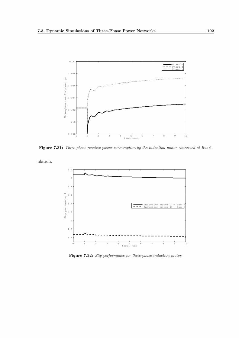
7.3. Dynamic Simulations of Three-Phase Power Networks 192
0 1 2 3 4 5 6 7 8 9 100.498
0.5
0.502
0.504
0.506
0.508
0.51
time, min
Thre
e−ph
ase
reac
tive
pow
er, p
uPhase aPhase bPhase c
Figure 7.31: Three-phase reactive power consumption by the induction motor connected at Bus 6.
ulation.
0 1 2 3 4 5 6 7 8 9 10
4.6
4.8
5
5.2
5.4
5.6
5.8
6
6.2
time, min
Slip
per
form
ance
, %
Induction motor 1 − Bus 5Induction motor 2 − Bus 6
Figure 7.32: Slip performance for three-phase induction motor.

7.3. Dynamic Simulations of Three-Phase Power Networks 193
0 1 2 3 4 5 6 7 8 9 100.985
0.99
0.995
1
1.005
1.01
time, min
Phase a
0 1 2 3 4 5 6 7 8 9 100.985
0.99
0.995
1
1.005
1.01
time, minVoltage magnitude, pu
Phase b
0 1 2 3 4 5 6 7 8 9 100.985
0.99
0.995
1
1.005
1.01
time, min
Phase c
Figure 7.33: Voltage magnitude for induction motor-connected buses.
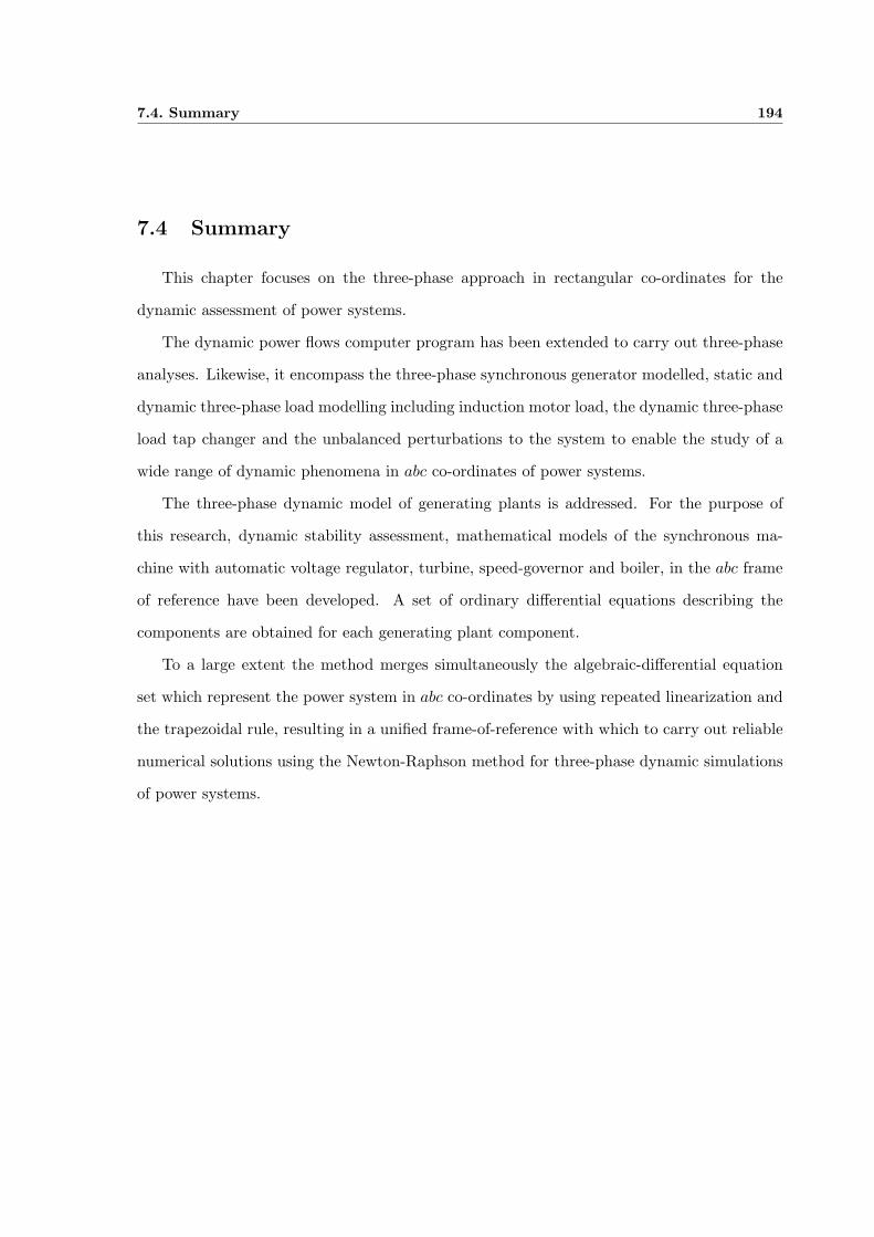
7.4. Summary 194
7.4 Summary
This chapter focuses on the three-phase approach in rectangular co-ordinates for the
dynamic assessment of power systems.
The dynamic power flows computer program has been extended to carry out three-phase
analyses. Likewise, it encompass the three-phase synchronous generator modelled, static and
dynamic three-phase load modelling including induction motor load, the dynamic three-phase
load tap changer and the unbalanced perturbations to the system to enable the study of a
wide range of dynamic phenomena in abc co-ordinates of power systems.
The three-phase dynamic model of generating plants is addressed. For the purpose of
this research, dynamic stability assessment, mathematical models of the synchronous ma-
chine with automatic voltage regulator, turbine, speed-governor and boiler, in the abc frame
of reference have been developed. A set of ordinary differential equations describing the
components are obtained for each generating plant component.
To a large extent the method merges simultaneously the algebraic-differential equation
set which represent the power system in abc co-ordinates by using repeated linearization and
the trapezoidal rule, resulting in a unified frame-of-reference with which to carry out reliable
numerical solutions using the Newton-Raphson method for three-phase dynamic simulations
of power systems.
Chapter 8
Conclusions
The dynamic assessment of electrical power systems using the Newton-Raphson method
represents the main concern in this research work. The goal is to develop suitable dy-
namic models of power plant components, such as synchronous generators, power loads,
VSC-FACTS controllers, and to assess their interaction with the electrical power network.
The solution technique makes use of a simultaneous solution approach which allows for
models of rotor saliency, flux decay, non-linear loads and a wide range of control actions to
be incorporated within a unified framework. This method is particulary suitable for carrying
out long-range dynamic assessments, which is one of the key points of concern of this thesis.
This contrast with more traditional solution techniques, namely, partitioned methods, which
are primarily aimed at covering short-range simulation studies.
This research work may be seen to consist of three main parts, which are: (i) Steady-state
power flows analysis in phase domain co-ordinates, including LCC-HVDC converters with
various control modes; (ii) dynamic power flows using a simultaneous solution technique,
including electro-mechanical controlled power plant components and VSC-FACTS devices
representation; (iii) and three-phase dynamic power flows for carrying out dynamic stability
assessments of unbalanced power systems.
8.1. Future work 196
From the dynamic simulation studies carried out, it has been observed that inclusion of
the load tap-changer transformer has the capability of enhancing system voltage stability. It
has also been assessed via modelling and simulation, that the voltage dependency of loads is a
matter of great importance in long-term dynamic phenomena and that the load models should
reflect such dependency correctly when carrying out long-term dynamic studies. Indeed,
the studies carried out show that the most realistic way of load modelling representation
during voltage stability assessments is when induction motor loads are modelled explicitly as
induction motors and not by static polynomial loads with voltage exponent 1.
The inclusion of VSC-FACTS controllers have shown to contribute effectively to providing
dynamic voltage support during steady-state operation, and to enhance power system stabil-
ity under unfavourable conditions. They have a faster response speeds than those provided
by electromechanical devices.
Quantifiable outcome of this research, are software environments for carrying out com-
prehensive dynamic power flows studies in both positive sequence and in abc co-ordinates.
Using the generated software, detailed simulations have been carried out in order to assess
the dynamic impact of various power plant components on the electrical power network.
Dynamic modelling of the system is amenable to its better understanding, particularly
when it undergoes unfavourable conditions.
It is worth adding that with the ever-increasing power of computers, the development
of real-time simulators for dispatching and security monitoring issues are finding increasing
favour, and that simulation tools using the same philosophy as that applied in this research
work may be used as the core of an on-line dynamic security assessment application system.
8.1 Future work
Alongside the developed mathematical models for VSC-FACTS devices and its inclusion
into the simultaneous method for carrying out dynamic stability assessments for electrical

8.1. Future work 197
power networks, more work needs to be done for including models of additional power elec-
tronics controllers such as the UPFC and the TCSC. Modelling of embedded generation tech-
nologies should be considered for its incorporation into the dynamic power flow algorithm,
including wind farms.

Bibliography
(2007). ABB.
Acha, E., Fuerte-Esquivel, C., Ambriz-Perez, H., and Angeles-Camacho, C. (2004). FACTS
Modelling and Simulation in Power Networks. John Wiley & Sons, Inc.
Ainsworth, J. D. (1988). Phase-locked oscillator control system for thyristor-controlled reac-
tors. IEE Generation, Transmission and Distribution, 135(2):146–156.
Anderson, G., Donaleck, P., Farmer, R., Hatziargyriou, N., Kamwa, I., Kundur, P., Martins,
N., Paserba, J., Pourbeis, P., Sanches-Gasca, J., Schulz, R., Stankovic, A., Taylor, C.,
and Vittal, V. (2005). Causes of the 2003 Major Grid Blackout in North America and
Europe, and Recommended Means to Improve System Dynamic Performance. IEEE
Transaction on Power Systems, 20(4):1922–1928.
Anderson, P. M. and Fouad, A. A. (1997). Power System Control and Stability. IEEE Press.
Anrborg, S., Andersson, G., Hill, D., and Hiskens, I. (1998). On Influence of Load Mod-
ellling for Undervoltage Load Shedding Studies. IEEE Transaction on Power Systems,
13(13):395–400.
Arrillaga, J. (1998). High Voltage Direct Current Transmission. IEE Power and Energy
Series.
198
BIBLIOGRAPHY 199
Arrillaga, J. and Arnold, C. P. (1990). Computer Analysis of Power Systems. John Wiley &
Sons, Inc.
Arrillaga, J. and Callaghan, C. D. (1991). Three phase ac-dc load and harmonics flows. IEEE
Transactions on Power Delivery, 6:238–241.
Arrillaga, J., Liu, Y. H., and Watson, N. R. (2007). Flexible Power Transmission. The HVDC
Option. John Wiley & Sons, Inc.
Arrillaga, J. and Watson, N. R. (2001). Computer Modelling of Electrical Power Systems.
John Wiley & Sons, Inc, second, edition.
Arrillaga, J. and Watson, N. R. (2002). Power Systems Electromagnetic Transients Simula-
tion. The IET, first edition.
Bahrman, M. P. and Johnson, B. K. (2007). The ABCs of HVDC Transmission Technologies.
IEEE Power & Energy Magazine, 5(2):32–44.
Banerjee, S. and Verghese, G. C. (2001). Nonlinear Phenomena in Power Electronics. Wiley-
IEEE Press.
Carlsson, L. (2002). Classical HVDC: Still continuing to evolve. Modern Power Systems,
MPS Review: Transmission & Distribution, pages 19–21.
Chapman, S. (1991). Electric Machinery Fundamentals. McGraw Hill, Inc, second edition.
Chen, M.-S. and Dillon, W. E. (1974). Power system modeling. Proceedings of the IEEE,
62(7):901–915.
Chow, J. H. (1982). Time-Scale Modeling of Dynamic Networks with Applications to Power
Systems. Springer-Verlag.
Cole, S., Hertem, D. V., Pardon, I., and Belmans, R. (2006). Randstad HVDC. Technical
report, Research Group Electa.
BIBLIOGRAPHY 200
Concordia, C. (1951). Synchronous Machines. Theory and performance. John Wiley & Sons,
Inc.
Concordia, C. and Ihara, S. (1982). Load Representation in Power system Stability Studies.
IEEE Transaction, PAS-101:969–977.
Corwin, L. and Miles, W. (1998). Impact assessment of the 1977 new york city blackout.
Technical report, System Control Inc., Energy Division.
Dommel, H. W. and Sato, N. (1972). Fast transient solutions. IEEE Transactions on Power
Apparatus and Systems, 91:1643–1650.
Elgerd, O. (1971). Electric Energy System Theory: An Introduction. McGraw Hill.
Energy Development and Power Generating Committe of the PES (2003). IEEE Recom-
mended Practice for Excitation System Models for Power System Stability Studies.
Gear, C. W. (1971a). Numerical Initial Value Problem in Ordinary Differential Equations.
Prentice Hall.
Gear, C. W. (1971b). Simultaneous numerical solution of differential-algebraic equations.
IEEE Transactions on Circuit Theory, 18:89–95.
Hagajos, L. and Danai, B. (1998). Laboratory measurements and models of modem loads
and their effect on voltage stability studies. IEEE Transactions on Power Systems,
13(2):584–592.
Harker, B. J. and Arrillaga, J. (1979). 3-phase ac-dc load flow. IEE Proceedings, 126:1275–
1281.
Hill, D. (1993). Nonlinear Dynamic Load Models with Recovery for Voltage Stability Studies.
IEEE Transaction on Power Systems, 8(1):166–176.
BIBLIOGRAPHY 201
Hill, D. and Mareels, I. (1990). Stability Theory for Differential/Algebraic Systems with
Application to Power Systems. IEEE Transaction on Circuits and Systems, 37(11):1416–
1423.
Hingorani, N. G. and Gyugyi, L. (1999). Understanding FACTS. Concept and Technology of
Flexible AC Transmission Systems. John Wiley & Sons, Inc.
IEEE Committee Report (1973). Dynamic Models for Steam and Hydro Turbines in Power
System Studies. IEEE Transactions on Power Apparatus and Systems, 92:1904–1915.
IEEE Committee Report (1981). Excitation System models for Power System Stability Stud-
ies. IEEE Transactions on Power Apparatus and Systems, 100:494–509.
IEEE Power Engineering Society (2002). Voltage Stability Assessment: Concepts, Practices
and Tools”, Final document.
Johansson, S. G., Asplund, G., Jansson, E., and Rudervall, R. (2004). Power System Stability
Benefits with VSC DC-Transmission Systems. Technical Report B4-204, CIGRE.
Kassakian, J., Schlecht, M., and Verghese, G. C. (1991). Principles of Power Electronics.
Addison-Wesley.
Kimbark, E. W. (1948a). Power System Stability, volume 1, Elements of Stability Calculation.
IEEE Press.
Kimbark, E. W. (1948b). Power System Stability, volume 3, Synchronous Machines. IEEE
Press.
Knight, U. G. (2001). Power Systems in Emergencies: From Contigency Planning to Crisis
Management. John Wiley & Sons, Inc.
Kundur, P. (1994). Power System Stability and Control. McGraw Hill.
BIBLIOGRAPHY 202
Lapidus, L. and Seinfeld, J. (1971). Numerical Solution of Ordinary Differential Equations.
Academic Press.
Lehn, P. W. and Iravani, M. R. (1998). Experimental evaluation of STATCOM closed loop.
IEEE Transaction on Power Delivery, 13(4):1378–1384.
Lehn, P. W. and Iravani, M. R. (2002). Exact modeling of the voltage source converter. IEEE
Transaction on Power Delivery, 17(1):217–222.
Machowski, J., Bialek, J. W., and Bumby, J. R. (1997). Power System Dynamic and Stability.
John Wiley & Sons, Inc.
Milano, F. (2005). An open source power system analysis toolbox. IEEE Transactions on
Power Systems, 20:1199–1206.
Milano, F. (2006). An open source power system analysis toolbox. In IEEE Power Engineer-
ing Society General Meeting. IEEE.
Milano, F. (2007). Psat version 2.
Morison, G. K., Gao, B., and Kundur, P. (1993). Voltge stability analysis using static and
dynamic approaches. IEEE Transactions on Power Systems, 8(3):1159–1171.
Nabavi-Niaki, S. A. (1996). Modelling and Applications of Unified Power Flow Controller
(UPFC) for Power Systems. Ph.d. thesis, University of Toronto.
Nasar, S. and Trutt, F. (1999). Electric Power Systems. CRC Press.
Padiyar, K. R. and Kulkarni, A. M. (1997). Design of reactive current and voltage controller
of static condenser. Electrical Power & Energy Systems, 19(6):397–410.
Park, R. H. (1929). Two-reaction theory of synchronous machines - generalized method of
analysis part i. AIEE Transactions, 48(2):716–730.
BIBLIOGRAPHY 203
Pavella, M. and Murthy, P. G. (1995). Transient Stability of Power Systems, Theory and
Practice. John Wiley & Sons, Inc.
Pedra, J., Sainz, L., and Corcoles, F. (2005). Study of aggregate models for squirrel-cage
induction motors. IEEE Transactions on Power Systems, 20:1519–1527.
Claudio A. Canizares (1995). On bifurcation, voltage collapse and load modelling. IEEE
Transactions on Power Systems, 10(1):512–522.
Commission de Regulation de L’energie (2004). Report on the event of september 28th, 2003
culminating in the separation of the italian power system from the ohter ucte networks.
Technical report, Commission de Regulation de L’energie and Autorita per l’energia
elettrica e il gas.
IEEE (2000). Special issues on hybrid systems. IEEE Proceedings, 88(7):879–887.
IEEE Load Task Force (1993). Load representation for dynamic performance analysis [of
power systems]. IEEE Transactions on Power Systems, 8:472–482.
IEEE Power Engineering Review (1991). Northeast blackout of 1965. Technical report, IEEE.
IEEE Task Force on Load Representation (1995). Load models for power flow and dynamic
performance simulation. IEEE Transaction on Power Systems, 10:523–538.
IEEE Working Group on Power Plant Response to Load Changes (1973). Mw response of
fossil fueled steam units. IEE Proceedings, PAS-92:455–463.
IEEE/CIGRE Joint Task Force on Stability Terms and Definitions (2004). Definition and clas-
sification of power system stability. IEEE Transactions on Power Systems, 19(2):1387–
1401.
National Grid (2003). Report into the august 28 2003 south london power failure. Technical
report, National Grid.
BIBLIOGRAPHY 204
US - Canada Power System Outage Task Force (2004). Final Report on the August 14, 2003
Blackout in the United States and Canada: Causes and Recommendations.
Qin, W., Hwachang, S., and Ajjarapu, V. (2006). Continuation-based quasi-steady-state
analysis. IEEE Transactions on Power Systems, 21(1):171–179.
Rafian, M., Sterling, M., and Irving, M. (1987). Real-time power system simulation. IEE
Proceedings, 134(3):209–223.
Rashid, M. H. and Maswood, A. I. (1988). Analysis of three-phase ac-dc converters under
unbalanced supply conditions. IEEE Transactions on Industry Applications, 24(3):449–
455.
Reed, G. and Takeda, M. (2003). Advantages of voltage source converters (vsc) based design
concepts for facts and hvdc-link applications. IEEE Power Engineering Society, General
Meeting, 13:1816–1821.
Sekine, Y. and Ohtsuki, H. (1990). Cascaded Voltage Collapse. IEEE Transaction on Power
Systems, 5(1):250–256.
Siemens AG Power Transmission and Distribution High Voltage Division (2007). High Voltage
Direct Current Transmission - Proven Technology for Power Exchange. available at:
www.nyri.us/pdfs.
Smed, E. T. (1989). A new approach to ac/dc power flow. Msc. thesis, Auburn University.
Smith, B. and Arrillaga, J. (1998). Improved three-phase load flow using phase and sequence
components. IEE Generation, Transmission and Distribution, 145(3):245–250.
Stagg, G. W. and El-Abiad, A. H. (1968). Computer Methods in Power Systems. McGraw
Hill.
Stevenson Jr, W. (1982). Elements of Power System Analysis. McGraw Hill, fourth edition.
BIBLIOGRAPHY 205
Stott, B. (1979). Power systems dynamic response calculations. IEEE Proceedings, 67:219–
241.
Stott, B. and Alsac, O. (1974). Fast decoupled load flow. IEEE Transactions on Power
Apparatus and Systems, 93(3):745–751.
Taylor, C. W. (1994). Power System Voltage Stability. McGraw Hill.
Tinney, W. F. and Hart, C. E. (1967). Power flows solution by newton method. IEEE
Transactions on Power Apparatus and Systems, 86(11):1449–1460.
Van Cutsem, T. and Vournas, C. (1998). Voltage Stability of Electric Power Systems. Kluwer
Academic Publishers.
Weedy, B. M. (1967). Electric Power Systems. John Wiley & Sons, Inc.
Williams, P. (1972). Numerical Computation. T. Nelson & Sond Ltd.
Wilsun Xu, J. R. M. and Dommel, H. W. (1991). A multiphase harmonic load flow solution
technique. IEEE Transactions on Power Systems, 6(1):174–182.
Xu, W. and Mansour, Y. (1994). Voltage stability analysis using generic dynamic load models.
IEEE Transactions on Power Systems, 9(1):479–486.
Zhang, L., Harnefors, L., and Rey, P. (2007). Power System Reliability and Transfer Capa-
bility Improvement by VSC-HVDC (HVDC Light). Security and Realibility of Electric
Power Systems, CIGRE Regional Meeting:1–7.
Zhang, X.-P. (1996). Fast three-phase load flow method. IEEE Transactions on Power
Systems, 11(3):1547–1554.
Zhang, X.-P., Ju, P., and Handschin, E. (2005). Continuation three-phase power flow: A tool
for voltage stability analisys of unbalanced three-phase power systems. IEEE Transac-
tions on Power Systems, 20(3):1320–1329.
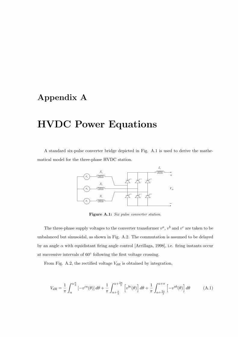
Appendix A
HVDC Power Equations
A standard six-pulse converter bridge depicted in Fig. A.1 is used to derive the mathe-
matical model for the three-phase HVDC station.
Ls
Xa
Xc
Xb
ea
ec
eb V
dR
+
_
Figure A.1: Six pulse converter station.
The three-phase supply voltages to the converter transformer va, vb and vc are taken to be
unbalanced but sinusoidal, as shown in Fig. A.2. The commutation is assumed to be delayed
by an angle α with equidistant firing angle control [Arrillaga, 1998], i.e. firing instants occur
at successive intervals of 60◦ following the first voltage crossing.
From Fig. A.2, the rectified voltage VdR is obtained by integration,
VdR =1π
∫ α π3
α[−vca(θ)] dθ +
1π
∫ α+ 2π3
α+π3
[vbc(θ)
]dθ +
1π
∫ α+π
α+ 2π3
[−vab(θ)
]dθ (A.1)

207
Figure A.2: Unbalanced converter voltage waveform.
The voltage VdR is made up of three terms,
VdR = V adR + V b
dR + V cdR (A.2)
where
V adR =
A√
2V ab
π
[cos
(α +
π
3
)− cos
(α +
2π
3
)](A.3)
V bdR =
A√
2V bc
π
[cos
(α + θbc − π
)− cos
(α + θbc − 2π
3
)](A.4)
V cdR =
A√
2V ca
π
[cos
(α + θca − π
3
)− cos (α + θca)
](A.5)
giving
V ρdR
Ak
√2V ρ
k
πcos (α + Aρ) (A.6)
208
where
Aa = θab = 0
Ab = θbc − 4π3
Ac = θca − 2π3
A similar expression is developed for the inverter,
V ρdI =
Am
√2V ρ
m
πcos (γ + Bρ) (A.7)
where
Ba = ϕab = 0
Bb = ϕbc − 4π3
Bc = ϕca − 2π3
Taking into account the voltage drop ∆V , the DC voltages of the rectifier and the inverter
are:
V ρdR =
Ak
√2V ρ
k
πcos (α + Aρ)−∆V (A.8)
V ρdI =
Am
√2V ρ
m
πcos (γ + Bρ)−∆V (A.9)
where ∆V is defined as,
∆V =XcId
π(A.10)
The powers of the inverter and the rectifier are given by the following expressions,

209
PdR = VdRId =∑
ρ=a,b,c
V ρdRId (A.11)
PdI = VdIId =∑
ρ=a,b,c
V ρdIId (A.12)
The relations between the currents on the primary side of the three-phase transformers
and the direct current Id, are given by,
Iρk = Akk
√6
πId = AkkId
Iρm = Amk
√6
πId = AmkId
(A.13)
where k is a constant associated with commutation overlap. For power flow analysis, it
can be taken to be k = 0.995 [Arrillaga and Arnold, 1990].
The apparent powers are given by,
Sρk =
V ρk Iρ
k√3
=k1AkV
ρk Id√
3(A.14)
Sρm =
V ρmIρ
m√3
=k1AmV ρ
mId√3
(A.15)
where
k1 =√
6π k

Appendix B
Jacobian Matrix Elements
B.1 Jacobian Elements - Partial Derivatives
The Jacobian matrix elements corresponding to the discretised differential equations for
the transient synchronous generators model are described as follow.
The non-zero partial derivatives corresponding to the function Fω(t) are:
∂Fω(t)
∂ω= 1 + KD (B.1)
∂Fω(t)
∂δ= 2Kx′qIrIm sin 2δ − 2Kx′dIrIm sin 2δ + KE′
qIm cos δ
−Kx′dI2r cos 2δ + KE′
dIm sin δ −KE′qIr sin δ
+KE′dIr cos δ + KX ′
qI2r cos 2δ −Kx′qI
2m cos δ + Kx′dI
2m cos 2δ (B.2)
∂Fω(t)
∂E′d
= K (Ir sin δ − Im cos δ) (B.3)
∂Fω(t)
∂E′q
= K (Ir cos δ + Im sin δ) (B.4)
B.2. Discretised State Variables 211
The non-zero partial derivatives corresponding to the function Fδ(t) are:
∂Fδ(t)
∂ω= −dt
2(B.5)
∂Fδ(t)
∂δ= 1 (B.6)
The non-zero partial derivatives corresponding to the function FE′d(t)
are:
∂FE′d(t)
∂δ=
12dtT ′q
(x′q − xq
)− Ir sin δ + Im cos δ (B.7)
∂FE′d(t)
∂E′d
= 1 +1
2dtT ′q(B.8)
The non-zero partial derivatives corresponding to the function FE′q(t)
are:
∂FE′q(t)
∂δ= − 1
2dtT ′d
(x′d − xd
)+ Ir cos δ + Im sin δ (B.9)
∂FE′q(t)
∂E′q
= 1 +1
2dtT ′d(B.10)
The Jacobian matrix elements corresponding to the discretised differential equations for
power plant components are described as follow.
B.2 Discretised State Variables
The armature resistance and damping coefficient of generator are considered so, the gen-
erator power output is therefore of the form,
Pe =ra |E|2r2a + x2
d
− |E| [ra (e cos δ + f sin δ) + xd (f cos δ + e sin δ)]r2a + x2
d
(B.11)

B.2. Discretised State Variables 212
The application of the trapezoidal rule to Eq.4.6 and Eq.4.9 are described as follows.
The electromechanical differential equation for the speed is ω = πfo
H [Pm − Pe −D (ω − ωo)]
so, the application of the trapezoidal rule to this Equation is,
ωt = ωt−∆t +∆t
2(ω(t) + ω(t−∆t)
)(B.12)
Ft(ω) + Ft−∆t(ω) + Cte = 0 (B.13)
then,
Ft−∆t (ω) = −ωt−∆t−∆t
2
{πf0
H
[(PHP (t−∆t)FHP + PIP (t−∆t)FIP + PLP (t−∆t)FLP
)− ra
∣∣E(t−∆t)
∣∣2r2a + x2
d
+
∣∣E(t−∆t)
∣∣ [−ra
(e(t−∆t) cos δ(t−∆t) + f(t−∆t) sin δ(t−∆t)
)
r2a + x2
d
+
xd
(−f(t−∆t) cos δ(t−∆t) + e(t−∆t) sin δ(t−∆t)
)]
r2a + x2
d
−D(ω(t−∆t))
]}(B.14)
Ft (ω) = ωt − ∆t
2
{πf0
H
[(PHP (t)FHP + PIP (t)FIP + PLP (t)FLP
)− ra
∣∣E(t)
∣∣2r2a + x2
d
+
∣∣E(t)
∣∣ [−ra
(e(t) cos δ(t) + f(t) sin δ(t)
)+ xd
(−f(t) cos δ(t) + e(t) sin δ(t)
)]
r2a + x2
d
−D(ω(t))
]}(B.15)
Cte = −∆tπf0
H(Dωo) (B.16)
B.2. Discretised State Variables 213
A similar process is applied to Eq. 4.9, for this Equation we have that,
δ(t) − δ(t−∆t) −∆t
2
(δ(t) + δ(t−∆t)
)= 0 (B.17)
where,
Ft−∆t (δ) = −δ(t−∆t) −∆t
2ω(t−∆t) (B.18)
Ft (δ) = δ(t) −∆t
2ω(t) (B.19)
C2 = 2πf0∆t (B.20)
For Pg, we have,
F (Pg) = Ft (Pg) + Ft−∆t (Pg) + Cte (B.21)
Pg(t) − Pg(t−∆t) −∆t
2
(Pg(t) + Pg(t−∆t)
)= 0 (B.22)
Pg(t) − Pg(t−∆t) −∆t
2
{1T3
(Pset(t) − P1(t) − Pg(t)
)+
1T3
(Pset(t) − P1(t) − Pg(t)
)}(B.23)
Ft−∆t (Pg) = −Pg(t−∆t) −∆t
2
{1T3
(−P1(t−∆t) − Pg(t−∆t)
)}(B.24)
Ft (Pg) = Pg(t) −∆t
2
{1T3
(−P1(t) − Pg(t)
)}(B.25)
B.2. Discretised State Variables 214
Cte = −∆tPset
T3(B.26)
The discretisation for these elements is like,
F (E) = Ft (E) + Ft−∆t (E) + Cte (B.27)
E(t) −E(t−∆t) −∆t
2
(E1(t) + E1(t−∆t)
)= 0 (B.28)
E(t) − E(t−∆t) −∆t
2
KAVref −KA
√(e2
(t) + f2(t))−E(t)
T ′d0
−∆t
2
KAVref −KA
√(e2
(t−∆t) + f2(t−∆t))− E(t−∆t)
T ′d0
= 0 (B.29)
Ft (E) = E(t) −∆t
2
−KA
√(e2
(t) + f2(t))− E(t)
T ′d0
(B.30)
Ft−∆t(E) = −E(t−∆t) −∆t
2
−KA
√(e2
(t−∆t) + f2(t−∆t))− E(t−∆t)
T ′d0
(B.31)
Cte = −∆t
(VrefKA
T ′d0
)(B.32)
The same process is applied to the remaining state variables of the system.

Appendix C
Power Networks Test Data
Following the data for the power system test networks used are depicted. All data is given
in per unit on a 100 MW and 400 kV base values of active power and voltage respectively.
Table C.1: Transmission line parameters: Five-bus test systemBus code Impedance Line charging
North South 0.02+ j0.06 0.00+ j0.06North Lake 0.08+ j0.24 0.00+ j0.05South Lake 0.06+ j0.18 0.00+ j0.04South Main 0.06+ j0.18 0.00+ j0.04South Elm 0.04+ j0.12 0.00+ j0.03Lake Main 0.01+ j0.03 0.00+ j0.02Main Elm 0.08+ j0.24 0.00+ j0.05
Table C.2: Generation: Five-bus test systemBus code MW MVAR MVAR limits Voltage magnitudeNorth* – – – 1.06South 40 0 ±300 1.00
* Slack bus
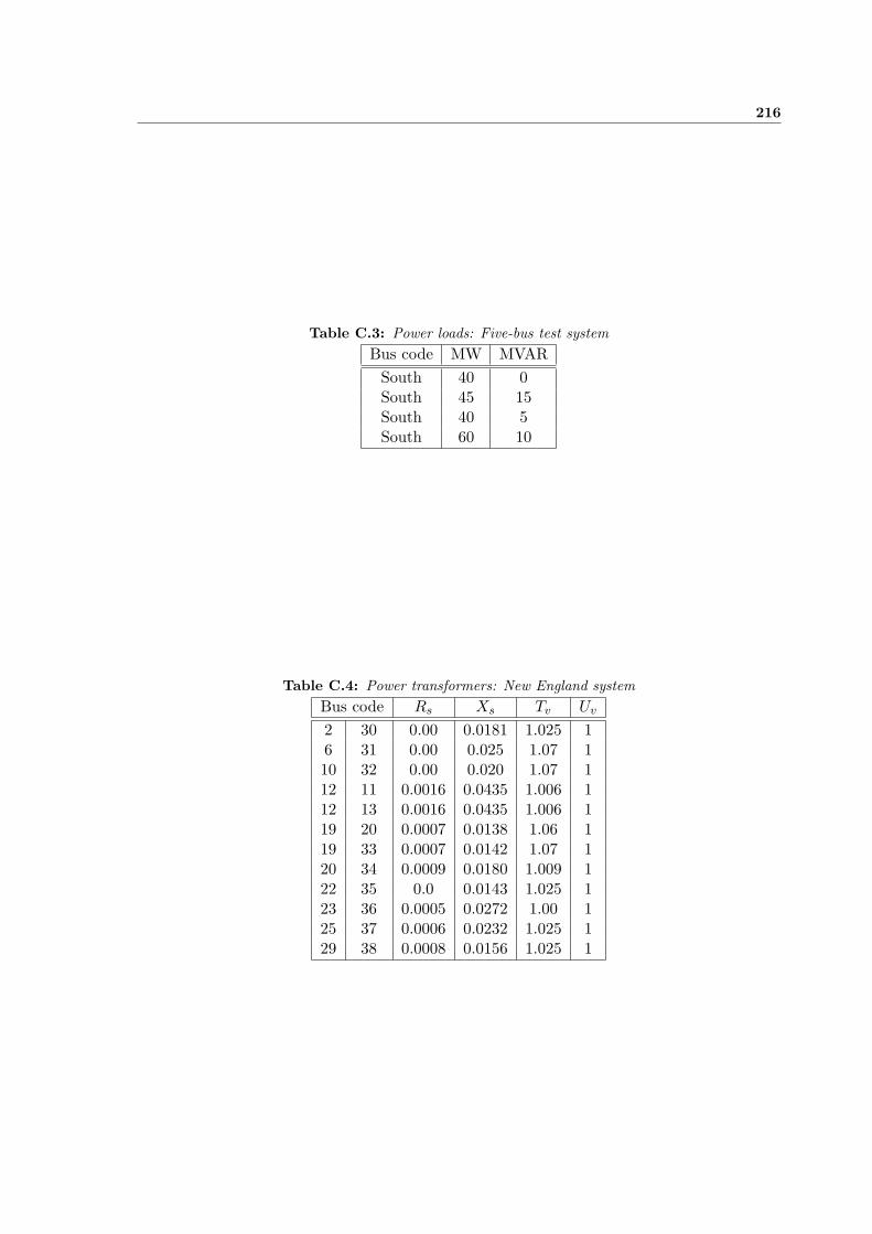
216
Table C.3: Power loads: Five-bus test systemBus code MW MVAR
South 40 0South 45 15South 40 5South 60 10
Table C.4: Power transformers: New England systemBus code Rs Xs Tv Uv
2 30 0.00 0.0181 1.025 16 31 0.00 0.025 1.07 110 32 0.00 0.020 1.07 112 11 0.0016 0.0435 1.006 112 13 0.0016 0.0435 1.006 119 20 0.0007 0.0138 1.06 119 33 0.0007 0.0142 1.07 120 34 0.0009 0.0180 1.009 122 35 0.0 0.0143 1.025 123 36 0.0005 0.0272 1.00 125 37 0.0006 0.0232 1.025 129 38 0.0008 0.0156 1.025 1
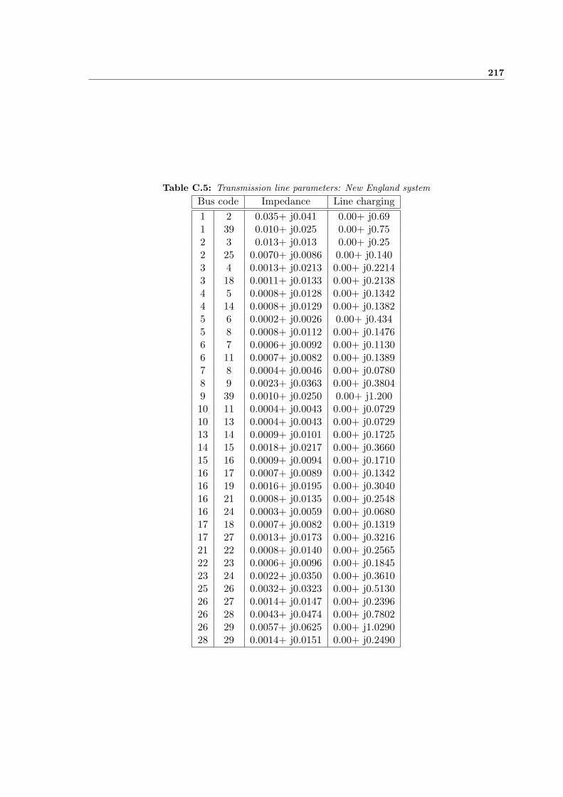
217
Table C.5: Transmission line parameters: New England systemBus code Impedance Line charging1 2 0.035+ j0.041 0.00+ j0.691 39 0.010+ j0.025 0.00+ j0.752 3 0.013+ j0.013 0.00+ j0.252 25 0.0070+ j0.0086 0.00+ j0.1403 4 0.0013+ j0.0213 0.00+ j0.22143 18 0.0011+ j0.0133 0.00+ j0.21384 5 0.0008+ j0.0128 0.00+ j0.13424 14 0.0008+ j0.0129 0.00+ j0.13825 6 0.0002+ j0.0026 0.00+ j0.4345 8 0.0008+ j0.0112 0.00+ j0.14766 7 0.0006+ j0.0092 0.00+ j0.11306 11 0.0007+ j0.0082 0.00+ j0.13897 8 0.0004+ j0.0046 0.00+ j0.07808 9 0.0023+ j0.0363 0.00+ j0.38049 39 0.0010+ j0.0250 0.00+ j1.20010 11 0.0004+ j0.0043 0.00+ j0.072910 13 0.0004+ j0.0043 0.00+ j0.072913 14 0.0009+ j0.0101 0.00+ j0.172514 15 0.0018+ j0.0217 0.00+ j0.366015 16 0.0009+ j0.0094 0.00+ j0.171016 17 0.0007+ j0.0089 0.00+ j0.134216 19 0.0016+ j0.0195 0.00+ j0.304016 21 0.0008+ j0.0135 0.00+ j0.254816 24 0.0003+ j0.0059 0.00+ j0.068017 18 0.0007+ j0.0082 0.00+ j0.131917 27 0.0013+ j0.0173 0.00+ j0.321621 22 0.0008+ j0.0140 0.00+ j0.256522 23 0.0006+ j0.0096 0.00+ j0.184523 24 0.0022+ j0.0350 0.00+ j0.361025 26 0.0032+ j0.0323 0.00+ j0.513026 27 0.0014+ j0.0147 0.00+ j0.239626 28 0.0043+ j0.0474 0.00+ j0.780226 29 0.0057+ j0.0625 0.00+ j1.029028 29 0.0014+ j0.0151 0.00+ j0.2490
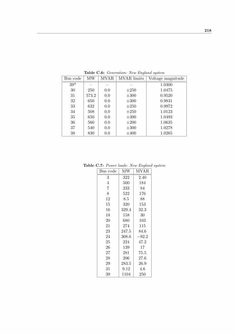
218
Table C.6: Generation: New England systemBus code MW MVAR MVAR limits Voltage magnitude
39* – – – 1.030030 250 0.0 ±250 1.047531 573.2 0.0 ±300 0.952032 650 0.0 ±300 0.983133 632 0.0 ±250 0.997234 508 0.0 ±250 1.012335 650 0.0 ±300 1.049336 560 0.0 ±200 1.063537 540 0.0 ±300 1.027838 830 0.0 ±400 1.0265
Table C.7: Power loads: New England systemBus code MW MVAR
3 322 2.404 500 1847 233 848 522 17612 8.5 8815 320 15316 329.4 32.318 158 3020 680 10321 274 11523 247.5 84.624 308.6 −92.225 224 47.226 139 1727 281 75.528 206 27.629 283.5 26.931 9.12 4.639 1104 250
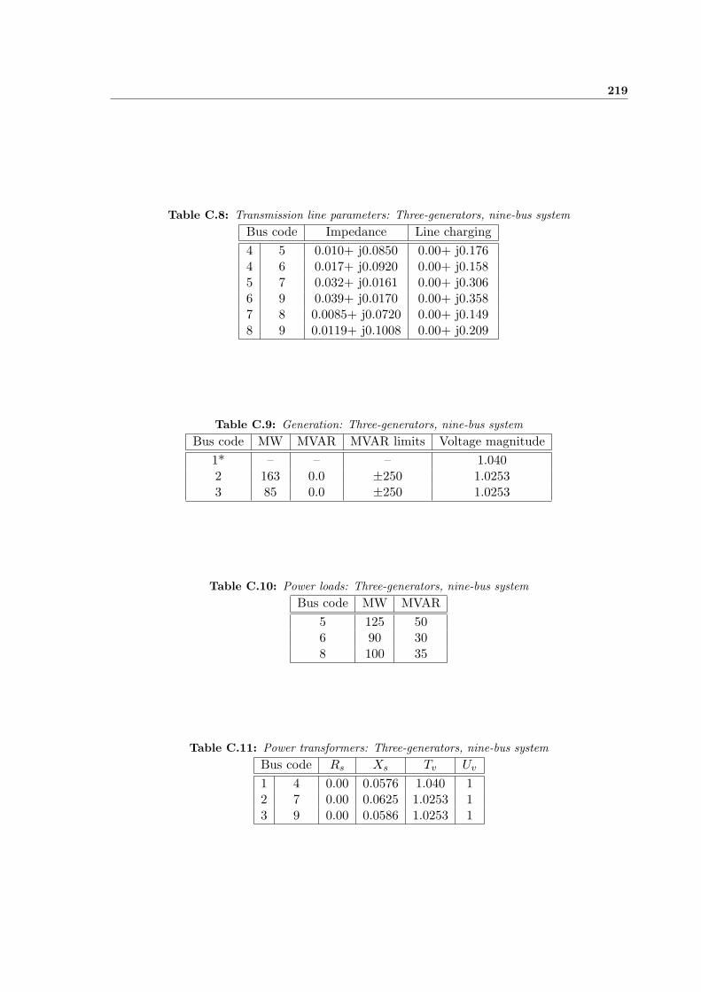
219
Table C.8: Transmission line parameters: Three-generators, nine-bus systemBus code Impedance Line charging4 5 0.010+ j0.0850 0.00+ j0.1764 6 0.017+ j0.0920 0.00+ j0.1585 7 0.032+ j0.0161 0.00+ j0.3066 9 0.039+ j0.0170 0.00+ j0.3587 8 0.0085+ j0.0720 0.00+ j0.1498 9 0.0119+ j0.1008 0.00+ j0.209
Table C.9: Generation: Three-generators, nine-bus systemBus code MW MVAR MVAR limits Voltage magnitude
1* – – – 1.0402 163 0.0 ±250 1.02533 85 0.0 ±250 1.0253
Table C.10: Power loads: Three-generators, nine-bus systemBus code MW MVAR
5 125 506 90 308 100 35
Table C.11: Power transformers: Three-generators, nine-bus systemBus code Rs Xs Tv Uv
1 4 0.00 0.0576 1.040 12 7 0.00 0.0625 1.0253 13 9 0.00 0.0586 1.0253 1