gap safe screening rules for sparsity enforcing...
TRANSCRIPT

Journal of Machine Learning Research 18 (2017) 1-33 Submitted 11/16; Revised 11/17; Published 11/17
Gap Safe Screening Rules for Sparsity Enforcing Penalties
Eugene Ndiaye [email protected], Telecom ParisTech, Universite Paris-Saclay, 75013, Paris, France
Olivier Fercoq [email protected], Telecom ParisTech, Universite Paris-Saclay, 75013, Paris, France
Alexandre Gramfort [email protected], Universite Paris-Saclay, 91120, Palaiseau, FranceLTCI, Telecom ParisTech, Universite Paris-Saclay, 75013, Paris, France
Joseph Salmon [email protected]
LTCI, Telecom ParisTech, Universite Paris-Saclay, 75013, Paris, France
Editor: David Wipf
Abstract
In high dimensional regression settings, sparsity enforcing penalties have proved useful toregularize the data-fitting term. A recently introduced technique called screening rules pro-pose to ignore some variables in the optimization leveraging the expected sparsity of thesolutions and consequently leading to faster solvers. When the procedure is guaranteed notto discard variables wrongly the rules are said to be safe. In this work, we propose a uni-fying framework for generalized linear models regularized with standard sparsity enforcingpenalties such as `1 or `1`2 norms. Our technique allows to discard safely more variablesthan previously considered safe rules, particularly for low regularization parameters. Ourproposed Gap Safe rules (so called because they rely on duality gap computation) cancope with any iterative solver but are particularly well suited to (block) coordinate descentmethods. Applied to many standard learning tasks, Lasso, Sparse-Group Lasso, multi-task Lasso, binary and multinomial logistic regression, etc., we report significant speed-upscompared to previously proposed safe rules on all tested data sets.
Keywords: Convex optimization, screening rules, Lasso, multi-task Lasso, sparse logisticregression, Sparse-Group Lasso
1. Introduction
The computational burden of solving high dimensional regularized regression problem hasled to a vast literature on improving algorithmic solvers in the last two decades. With theincreasing popularity of `1-type regularization ranging from the Lasso (Tibshirani, 1996) orgroup-Lasso (Yuan and Lin, 2006) to regularized logistic regression and multi-task learning,many algorithmic methods have emerged to solve the associated optimization problems (Kohet al., 2007; Bach et al., 2012). Although for the simple `1 regularized least square a specificalgorithm (e.g., the LARS (Efron et al., 2004)) can be considered, for more general formu-lations, penalties, and possibly larger dimensions, (block) coordinate descent has proved tobe an efficient strategy (Friedman et al., 2010).
c©2017 Ndiaye et al. .
License: CC-BY 4.0, see https://creativecommons.org/licenses/by/4.0/. Attribution requirements are providedat http://jmlr.org/papers/v18/16-577.html.

Ndiaye et al.
Our main objective in this work is to propose a technique that can speed-up any iterativesolver for such learning problems, and that is particularly well suited for (block) coordinatedescent method as this type of method can easily ignore useless coordinates1.
The safe rules introduced by El Ghaoui et al. (2012) for generalized `1 regularizedproblems, is a set of rules allowing to eliminate features whose associated coefficients areguaranteed to be zero at the optimum, even before starting any algorithm. Relaxing thesafe rule, one can obtain some additional speed-up at the price of possible mistakes. Suchheuristic strategies, called strong rules by Tibshirani et al. (2012) reduce the computationalcost using an active set strategy, but require multiple post-processing to check for featurespossibly wrongly discarded.
Another road to speed-up screening method has been pursued following the introductionof sequential safe rules (El Ghaoui et al., 2012; Wang et al., 2012; Xiang et al., 2014; Wanget al., 2014). The idea is to improve the screening thanks to the computation done fora previous regularization parameter as in homotopy/continuation methods. This scenariois particularly relevant in machine learning, where one computes solutions over a grid ofregularization parameters, so as to select the best one, e.g., by cross-validation. Never-theless, the aforementioned methods suffer from the same problem as strong rules, sincerelevant features can be wrongly disregarded. Indeed, sequential rules usually rely on theexact knowledge of certain theoretical quantities that are only known approximately. Es-pecially, for such rules to work one needs the exact dual optimal solution from the previousregularization parameter, a quantity (almost) never available to the practitioner.
The recent introduction of dynamic safe rules by Bonnefoy et al. (2015, 2014) has openeda new promising venue by performing variable screening, not only before the algorithmstarts, but also along the iterations. This screening strategy can be applied for any standardoptimization algorithm such as FISTA (Beck and Teboulle, 2009), primal-dual (Chambolleand Pock, 2011), augmented Lagrangian (Boyd et al., 2011). Yet, it is particularly relevantfor strategies that can benefit from support reduction or active sets (Kowalski et al., 2011;Johnson and Guestrin, 2015), such as coordinate-descent (Fu, 1998; Friedman et al., 2007,2010).
This paper contains a synthesis and a unified presentation of the methods introducedfirst for the Lasso in (Fercoq et al., 2015) and then for `1`2 norms in (Ndiaye et al., 2015)as well as for Sparse-Group Lasso in (Ndiaye et al., 2016b). Our so-called Gap Safe rules(because the screening rules rely on duality gap computations), improved on dynamic saferules for a broad class of learning problems with the following benefits:
• Gap Safe rules are easy to insert in existing solvers,
• they are proved to be safe and unify sequential and dynamic rules,
• they lead to improved speed-ups in practice w.r.t. previously known safe rules,
• they achieve fast variable identifications2.
1. By construction a method like LARS (Efron et al., 2004), that applies only to the Lasso case, cannotbeneficiate from screening rules.
2. more precisely, we identify faster the equicorrelation set, see Theorem 14
2

Gap Safe Screening Rules
Furthermore, it is worth noting that strategies also leveraging dual gap computationshave recently been considered to safely discard irrelevant coordinates: Shibagaki et al. (2016)have considered screening rules for learning tasks with both feature sparsity and samplesparsity, such as for `1-regularized SVM. In this case, some interesting developments havebeen proposed, namely safe keeping strategies, which allow to identify features and samplesthat are guaranteed to be active. Constrained convex problems such as minimum enclosingball can also be included as shown in Raj et al. (2016). The Blitz algorithm by Johnson andGuestrin (2015) aims to speed up working set methods using duality gaps computations;significant gains were also obtained in limited-memory and distributed settings.
We introduce the general framework of Gap Safe screening rules in Section 3; in Section 4we instantiate them on various strategies including static, dynamic and sequential ones, andshow how the Gap Safe methodology can encompass all of them. The converging natureof the Gap Safe rules is also discussed. In Section 5, we investigate the specific form ofour rules for standard machine learning models: Lasso, Group Lasso, Sparse-Group Lasso,logistic regression with `1 regularization, etc. Section 6 reports a comprehensive set ofexperiments on four different learning problems using either dense or sparse data. Resultsdemonstrate the systematic gain in computation time of the Gap Safe rules.
2. Notation and Background on Optimization
For any integer d P N, we denote by rds the set t1, . . . , du and byQJ the transpose of a matrixQ. Our observation vector is y P Rn where n represents the number of samples. The designmatrix X “ rx1, . . . , xns
J P Rnˆp has p explanatory variables (or features) column-wise,and n observations row-wise. For a norm Ω, we write BΩ the associated unit ball, ‖¨‖2 is the`2 norm (and x¨, ¨y for the associated inner product), ‖¨‖1 is the `1 norm, and ‖¨‖8 is the `8norm. The `2 unit ball is denoted by B2 (or simply B) and we write Bpθ, rq the `2 ball withcenter θ and radius r. For a vector β P Rp, we denote by supppβq the support of β (i.e., theset of indices corresponding to non-zero coefficients) and by ‖B‖2F “
řpj“1
řqk“1 B2
j,k the
Frobenius norm of a matrix B P Rpˆq. We denote ptq` “ maxp0, tq and ΠCp¨q the projectionoperator over a closed convex set C. The soft-thresholding operator STτ (at level τ ě 0) isdefined for any x P Rd by rSTτ pxqsj “ signpxjqp|xj | ´ τq`.
The parameter to recover is a vector β “ pβ1, . . . , βpqJ admitting a group structure. A
group of features is a subset g Ă rps and ng is its cardinality. The set of groups is denotedby G and we focus only on non-overlapping groups3 that form a partition of the set rps.We denote by βg the vector in Rng which is the restriction of β to the indices in g. Wewrite rβgsj the j-th coordinate of βg. We also use the notation Xg P Rnˆng to refer to thesub-matrix of X assembled from the columns with indices j P g and Xj when the groupsare a single feature, i.e., when g “ tju.
Some elements of convex analysis used in the following sections are introduced here.For a function f : Rd Ñ r´8,`8s, the Fenchel-Legendre transform4 of f , is the functionf˚ : Rd Ñ r´8,`8s defined by f˚puq “ supzPRdxz, uy ´ fpzq. The sub-differential ofa function f at a point x is denoted by Bfpxq. For a norm Ω over Rd, its dual normis written ΩD and is defined for any u P Rd by ΩDpuq “ maxΩpzqď1xz, uy. Note that in
3. Overlapping groups could be treated as well, some insight is given in Section 5.34. Such a transform is often referred to as the (convex) conjugate of a (convex) function
3

Ndiaye et al.
the case of a group-decomposable norm, one can check that ΩDpβq “ maxgPG ΩDg pβgq and
BΩpβq “ ΠgPGBΩgpβgq.
We remind below useful standard results from convex analysis:
Proposition 1 (Fermat’s Rule) (see (Bauschke and Combettes, 2011, Proposition 26.1)for a more general result) For any convex function f : Rd Ñ R:
x‹ P arg minxPRd
fpxq ðñ 0 P Bfpx‹q. (1)
Proposition 2 (Subdifferential of a Norm) (see (Bach et al., 2012, Proposition 1.2))The sub-differential of the norm Ω at x, is given by
BΩpxq “
#
tz P Rd : ΩDpzq ď 1u “ BΩD , if x “ 0,
tz P Rd : ΩDpzq “ 1 and zJx “ Ωpxqu, otherwise.(2)
3. Gap Safe Framework
We propose to estimate the vector of parameters β by solving
βpλq P arg minβPRp
Pλpβq, for Pλpβq :“ F pβq ` λΩpβq :“nÿ
i“1
fipxJi βq ` λΩpβq , (3)
where all fi : R ÞÑ R are convex and differentiable functions with 1γ-Lipschitz gradientand Ω : Rp ÞÑ R` is a norm that is group-decomposable, i.e., Ωpβq “
ř
gPG Ωgpβgq whereeach Ωg is a norm on Rng . The λ parameter is a non-negative constant controlling thetrade-off between the data fitting term and the regularization term. Popular instantiationsof problems of the form (3) are detailed in Section 5.
Theorem 3 A dual formulation of the optimization problem defined in (3) is given by
θpλq “ arg maxθP∆X
´
nÿ
i“1
f˚i p´λθiq “: Dλpθq, (4)
where ∆X “ tθ P Rn : @g P G,ΩDg pX
Jg θq ď 1u. Moreover, the Fermat’s rule reads:
@i P rns, θpλqi “ ´∇fipxJi βpλqqλ plink equationq, (5)
@g P G, XJg θpλq P BΩgpβpλqg q psub-differential inclusionq. (6)
For any θ P Rn let us introduce Gpθq :“ r∇f1pθ1q, . . . ,∇fnpθnqsJ P Rn. Then the pri-mal/dual link equation can be written θpλq “ ´GpXβpλqqλ .
Contrarily to the primal, the dual problem has a unique solution under our assumptionon the fi’s. Indeed, the dual function is strongly concave, hence strictly concave.
4

Gap Safe Screening Rules
3.1 Safe Screening Rules
Following the seminal work by El Ghaoui et al. (2012) screening techniques have emerged asa way to exploit the known sparsity of the solution by discarding features prior to startinga sparse solver. Such techniques are referred to in the literature as safe rules when theyscreen out coefficients guaranteed to be zero in the targeted optimal solution. Zeroing thosecoefficients allows to focus exclusively on the non-zero ones (likely to represent signal) andhelps reducing the computational burden.
One well known extreme is the following: for λ ą 0 large enough, 0 is the unique solutionof (3). Indeed,
0 P arg minβPRp
F pβq ` λΩpβq(1)ðñ 0 P t∇F p0qu ` λBΩp0q
(2)ðñ ΩDp∇F p0qq ď λ.
Hence we recall the first “naive” screening rule, stating that for large values of the regular-ization parameter, all features can be discarded.
Proposition 4 (Critical Parameter: λmax) For any λ ą 0,
0 P arg minβPRp
Pλpβq ðñ λ ě λmax :“ ΩDp∇F p0qq “ ΩDpXJGp0qq .
So from now on, we will only focus on the case where λ ă λmax. In this case, screening rules
rely on a direct consequence of Fermat’s rule (6). If βpλqg ‰ 0, then ΩD
g pXJg θpλqq “ 1 thanks
to Equation (2). Since θpλq P ∆X , it implies, by contrapositive, that if ΩDg pX
Jg θpλqq ă 1 then
βpλqg “ 0. This relation means that the g-th group can be discarded whenever ΩD
g pXJg θpλqq ă
1. However, since θpλq is unknown — unless λ ą λmax, in which case θpλq “ Gp0qλ — thisrule is of limited use. Fortunately, it is often possible to construct a set R Ă Rn, called asafe region, that contains θpλq. This observation leads to the following result.
Proposition 5 (Safe Screening Rule El Ghaoui et al. (2012)) If θpλq P R, and g PG:
maxθPR
ΩDg pX
Jg θq ă 1 ùñ ΩD
g pXJg θpλqq ă 1 ùñ βpλqg “ 0 . (7)
The so-called safe screening rule consists in removing the g-th group from the problem
whenever the previous test is satisfied, since then βpλqg is guaranteed to be zero. Should R
be small enough to screen many groups, one can observe considerable speed-ups in practiceas long as the testing can be performed efficiently. A natural goal is to find safe regionsas narrow as possible: smaller safe regions can only increase the number of screened outvariables. To have useful screening procedures one needs:
• the safe region R to be as small as possible (and to contain θpλq),
• the computation of the quantity maxθPR
ΩDg pX
Jg θq to be cheap.
The later means that safe regions should be simple geometric objects, since otherwise,evaluating the test could lead to a computational burden limiting the benefits of screening.
5

Ndiaye et al.
3.2 Gap Safe Regions
Various shapes have been considered in practice for the safe region R such as balls (ElGhaoui et al., 2012), domes (Fercoq et al., 2015) or more refined sets (see Xiang et al. (2014)for a survey). Here we consider for simplicity the so-called “sphere regions” (following theterminology introduced by El Ghaoui et al. (2012)) choosing a ball R “ Bpθ, rq as a saferegion. Thanks to the triangle inequality, we have:
maxθPBpθ,rq
ΩDg pX
Jg θq ď ΩD
g pXJg θq ` max
θPBpθ,rqΩDg pX
Jg pθ ´ θqq,
and denoting ΩDg pXgq :“ supu‰0
ΩDg pXJg uq
‖u‖2the operator norm of Xg associated to ΩD
g p¨q, we
deduce from Proposition 7 the screening rule for the g-th group:
Safe sphere test: If ΩDg pX
Jg θq ` rΩ
Dg pXgq ă 1, then βpλqg “ 0 . (8)
3.2.1 Finding a Center
To create a useful center for a safe sphere, one needs to be able to create dual feasiblepoints, i.e., points in the dual feasible set ∆X . One such point is θmax :“ ´Gp0qλmax
which leads to the original static safe rules proposed by El Ghaoui et al. (2012). Yet, it hasa limited interest, being helpful only for a small range of (large) regularization parametersλ, as discussed in Section 4.1. A more generic way of creating a dual point that will be keyfor creating our safe rules is to rescale any point z P Rn such that it is in the dual set ∆X .The rescaled point is denoted by Θpzq and is defined by
Θpzq :“
#
z, if ΩDpXJzq ď 1,z
ΩDpXJzq, otherwise.
(9)
This choice guarantees that @z P Rn,Θpzq P ∆X . A candidate often considered for comput-ing a dual point is the (generalized) residual term z “ ´GpXβqλ. This choice is motivatedby the primal-dual link equation 5 i.e., θpλq “ ´GpXβpλqqλ.
3.2.2 Finding a Radius
Now that we have seen how to create a center candidate for the sphere, we need to find aproper radius, that would allow the associated sphere to be safe. The following theoremproposes a way to obtain a radius using the duality gap. The quantity
Gapλpβ, θq :“ Pλpβq ´Dλpθq (10)
is often referred to as the duality gap in the convex optimization literature, hence the nameof our proposed Gap Safe framework. This quantity is also a useful tool when designing astopping criterion: noting that for any β P Rp, θ P ∆X , Pλpβq ´ Pλpβ
pλqq ď Gapλpβ, θq, itsuffices to find a primal-dual pair with a duality gap smaller than ε to ensure an ε-accuracyprimal solution for Problem 3.
Theorem 6 (Gap Safe Sphere) Assuming that F has 1γ-Lipschitz gradient, we have
@β P Rp,@θ P ∆X ,∥∥∥θpλq ´ θ∥∥∥
2ď
d
2Gapλpβ, θq
γλ2. (11)
6

Gap Safe Screening Rules
Hence the set R “ Bpθ,a
2Gapλpβ, θqγλ2q is a safe region for any β P Rn and θ P ∆X .
Proof Remember that @i P rns, fi is differentiable with a 1γ-Lipschitz gradient. Asa consequence, @i P rns, f˚i is γ-strongly convex (Hiriart-Urruty and Lemarechal, 1993,Theorem 4.2.2, p. 83) and so the dual function Dλ is γλ2-strongly concave:
@pθ1, θ2q P Rn ˆ Rn, Dλpθ2q ď Dλpθ1q ` x∇Dλpθ1q, θ2 ´ θ1y ´γλ2
2‖θ1 ´ θ2‖22 .
Specifying the previous inequality for θ1 “ θpλq, θ2 “ θ P ∆X , one has
Dλpθq ď Dλpθpλqq ` x∇Dλpθ
pλqq, θ ´ θpλqy ´γλ2
2
∥∥∥θpλq ´ θ∥∥∥2
2.
By definition, θpλq maximizes Dλ on ∆X , so, x∇Dλpθpλqq, θ ´ θpλqy ď 0. This implies
Dλpθq ď Dλpθpλqq ´
γλ2
2
∥∥∥θpλq ´ θ∥∥∥2
2.
By weak duality @β P Rp, Dλpθpλqq ď Pλpβq, hence @β P Rp,@θ P ∆X , Dλpθq ď Pλpβq ´
γλ2
2 ‖θpλq ´ θ‖22 and the conclusion follows.
Remark 7 To build a Gap Safe region as in Equation (11), we only need strong convexityin the dual which is equivalent to smoothness of the loss function whereas the screening prop-erty (7), requires group separability of norms. Hence our framework of Gap Safe screeningrule automatically applies for a large class of problems.
Remark 8 During the review process, we became aware of a possible improvement for theradius Johnson and Guestrin (2016). In the Blitz framework, their approach leads to apotentially smaller radius, using a strongly concave upper bound of the dual function whosemaximum is known. In our framework, this can be used to improve the safe radius by a
?2
factor in the static case. This is unclear to us whether this can be done for the sequential anddynamic version. For the SVM problem Zimmert et al. (2015) got the same improvementby writing the duality gap as a function of primal variables only.
3.2.3 Safe Active Set
Note that any time a safe rule is performed thanks to a safe region R “ Bpθ, rq, one canassociate a safe active set Aθ,r, consisting of the features that cannot be removed yet by
the test in Equation (8). Hence, the safe active set contains the true support of βpλq.
Definition 9 (Safe Active Set) For a center θ P ∆X and a radius r ě 0, the safe(sphere) active set consists of the variables not eliminated by the associated (sphere) saferule, i.e.,
Apθ, rq :“ tg P G : ΩDg pX
Jg θq ` rΩ
Dg pXgq ě 1u . (12)
7

Ndiaye et al.
When choosing z “ ´GpXβqλ as proposed in Section 3.2.1 as the current residual,the computation of θ “ Θpzq in Equation (9) involves the computation of ΩDpXJzq. Astraightforward implementation would cost Opnpq operations. This can be avoided: whenusing a safe rule one knows that the index achieving the maximum for this norm is inApθ, rq. Indeed, by construction of the safe active set, it is easy to see that ΩDpXJzq “maxgPApθ,rqΩD
g pXJg zq. In practice the evaluation of the dual gap is therefore Opnqq where
q is the size of Apθ, rq. In other words, using a safe screening rule also speeds up theevaluation of the stopping criterion.
3.3 Outline of the Algorithm
When designing a supervised learning algorithm with sparsity enforcing penalties, the tuningof the parameter λ in Problem (3) is crucial and is usually done by cross-validation whichrequires evaluation over a grid of parameter values. A standard grid considered in theliterature is λt “ λmax10´δtpT´1q with a small δ, say δ “ 10´2 or 10´3, see for instance(Buhlmann and van de Geer, 2011)[2.12.1] or the glmnet package (Friedman et al., 2010).The parameter δ has an important influence on the computational burden: computing timetends to increase for small λ, the primal iterates being less and less sparse, and the problemto solve more and more ill-posed. It is customary to start from the largest regularizerλ0 “ λmax and then to perform iteratively the computation of βpλtq after the one of βpλt´1q.This leads to computing the models in the order of increasing complexity: this allowsimportant speed-up by benefiting of warm start strategies.
Here we propose a simple pathwise algorithm divided in two step:
• Active warm start: improve solver initialization by solving the problem restrictedto an initial estimation of the support based on sequential informations along theregularization path (see Section 4.4 for details on the various strategies investigated).
• Dynamic Gap Safe Screening: use the informations gained during the iterationsof the algorithm to obtain a smaller safe region therefore a greater elimination ofinactive variables (see Section 4.3).
We summarize our strategy for solving the problem given by Equation (3) in Algorithm 1 and2. The notation Solver p. . .q refers to any numerical solver that produces an approximationof the solution of (3) and SolverUpdate p. . .q is the updating scheme of the current vectoralong the iterations5. We consider solvers that can use a (primal) warm start point.
4. Screening strategies and theoretical analysis
We now describe the simplest safe rule strategy, which we refer to as the static strategy.
4.1 Static Safe Rules
The first static safe rule, introduced by El Ghaoui et al. (2012), discards variables beforeany computation thanks to Proposition 4. Here, the (safe) sphere is fixed once and for all,
5. For our experiments we have focused on (block) coordinate descent solvers
8

Gap Safe Screening Rules
Algorithm 1 Pathwise algorithm with active warm start
Input : X, y, ε, K, f ce, pλtqtPrT´1s
for t P rT ´ 1s do
β “ qβpλt´1q and // Get previous ε-solution
Get an initial (safe or not) support estimator S “ Spqβpλt´1qq
βS “ Solver pXS , y, βS , ε, K, fce, λtq // Active warm start
qβpλtq “ Solver pX, y, β, ε, K, f ce, λtq // Solve over all variables
Output:´
qβpλtq¯
tPrT´1s
Algorithm 2 Iterative solver with GAP safe rules: Solver pX, y, β, ε, K, f ce, λq
Input : X, y, β, ε, K, f ce, λ // Warm start is authorized here through β
for k P rKs doif k mod f ce “ 1 then
Compute a dual variable θ “ ´GpXβqmaxpλ,ΩDpXJGpXβqqqStop if Gapλpβ, θq ď ε
r “b
2Gapλpβ,θqγλ2 // Get Gap Safe radius as in Equation (11)
A “
g P G : ΩDg pX
Jg θq ` rΩ
Dg pXgq ě 1
(
// Get Safe active set as in Equation (12)
βA “ SolverUpdate pXA, y, βA, λq // Solve on current Safe active set
Output: qβpλq
hence the name static. The static rule reads:
Static sphere rule: If ΩDg pX
Jg θmaxq ` rmaxΩD
g pXgq ă 1, then βpλqg “ 0 ,
Center: θmax :“ ´Gp0qλmax ,
Radius: rmax :“a
2Gapλp0, θmaxqγλ2 .
There is a threshold λcritic such that for any λ smaller than λcritic the test from theStatic sphere rule can never be satisfied. This phenomenon appears clearly in the numericalexperiments presented in Section 6. In simple cases a closed form for λcritic can even beprovided. For instance, in the case of the Group Lasso, El Ghaoui et al. (2012) proposed
to use rmax “
∣∣∣ 1λ ´
1λmax
∣∣∣ ‖y‖2, and simple calculation gives:
λcritic :“ λmax ˆmingPG
‖y‖2 ΩDg pXgq
λmax ` ‖y‖2 ΩDg pXgq ´ ΩD
g pXgGp0qq.
4.2 Sequential Safe Rules
Provided that the λ’s are close enough along the regularization parameters, knowing anestimate of βpλt´1q gives a clever initialization to compute βpλtq. To initialize the solver fora new λt, a natural choice is to set the primal variable equal to βpλt´1q, an approximation ofβpλt´1q output by the solver (at a prescribed precision). This popular strategy is referred toas “warm start” in the literature (Friedman et al., 2007). On top of this standard strategy,
9

Ndiaye et al.
one can reuse prior dual information to improve the screening as well (El Ghaoui et al.,2012). This leads to the sequential strategy to screen for a new λt:
Sequential sphere rule: If ΩDg pX
Jg θpλt´1qq ` rtΩ
Dg pXgq ă 1, then βpλtqg “ 0 ,
Center: θpλt´1q :“ Θp´GpXβpλt´1qqλt´1q ,
Radius: rt :“b
2Gapλtpβpλt´1q, θpλt´1qqγλ2
t .
Remark 10 Previous works in the literature (Wang et al., 2012; Wang and Ye, 2014;Wang et al., 2014; Lee and Xing, 2014) proposed sequential safe rules, though they weregenerally used in an unsafe way in practice. Indeed, such rules relied on the exact knowledgeof θpλt´1q to screen out coordinates of βpλtq. Unfortunately, it is impossible to obtain sucha point6 since it is the solution of an optimization problem typically solved by an iterativesolver, hence such it is only known up to a limited precision. By ignoring such inaccuracyin the knowledge of θpλt´1q one can wrongly eliminate variables that do belong to the supportof βpλtq. Without a posteriori checking the screened out features, this could prevent thealgorithm from converging, as shown in (Ndiaye et al., 2016b, Appendix B).
4.3 Dynamic Safe Rules
Another road to speed up solvers using screening rules was proposed by Bonnefoy et al.(2014, 2015) under the name “dynamic safe rules”. For a fixed λ, it consists in performingscreening along with the iterations of the optimization algorithm used to solve Problem (3).Denoting by k the iteration number, they introduced a rule for the Lasso that consists of asafe sphere with center yλ and radius ‖yλ´ θk‖, where θk is a current dual feasible point.
Let us consider a sequence pβkq that converges to a primal solution βpλq. For creating adual feasible point, we apply the rescaling introduced in Equation (9) to z “ ´GpXβkqλand the dynamic strategy can be summarized by
Dynamic sphere rule: If ΩDg pX
Jg θkq ` rkΩ
Dg pXgq ă 1, then βpλqg “ 0 ,
Center: θk :“ Θp´GpXβkqλq defined thanks to (9) ,
Radius: rk :“a
2Gapλpβk, θkqγλ2 .
In practice the computation of the duality gap can be expensive due to the matrixvector operations needed to compute XJGpXβkq. For instance in the Lasso case, a dualgap computation requires almost as much computation as a full pass of coordinate descentover the data. Hence, it is recommended to evaluate the dynamic (safe) rule only everyfew passes over the data set. In all our experiments, we have set this screening frequencyparameter to f ce “ 10.
Note that contrary to the original dynamic screening rules proposed by Bonnefoy et al.(2014, 2015), the Gap Safe rules we introduced are converging in the sense that our saferegions converge to the singleton tθpλqu (see Section 4 for more details). Indeed, theirproposed safe sphere was centered on yλ, and their radius can only be greater than ‖yλ´θpλq‖ in the Lasso case they consider. We provide a visual comparison in Figure 1.
6. Except for λ0 “ λmax, where θmax :“ ´Gp0qλmax can be computed exactly
10

Gap Safe Screening Rules
(a) Bonnefoy et al. (2014) safe region (b) Gap Safe region
Figure 1: Illustration of safe region differences between Bonnefoy et al. (2014) and GapSafe strategies for the Lasso case; note that γ “ 1 in this case. Here β is a primalpoint, θ is a dual feasible point (the feasible region ∆X is in orange, while therespective safe balls R are in blue).
4.4 Active Warm Start
An another variant to further reduce running time in the active warm start, recentlyintroduced by Ndiaye et al. (2016a) for speeding-up concomitant Lasso computations.Instead of simply leveraging the previous primal solution, the active warm start strat-egy also makes use of the previous safe active set Apθt´1, rt´1q, with θt´1 “ θpλt´1q andrt´1 “ rλt´1pβ
pλt´1q, θpλt´1qq. The idea is to take as a new primal warm start point, the(approximate) minimizer of Pλt under the additional constraint that its support is includedin the safe active set Apθt´1, rt´1q i.e.,
rβpλt´1,λtq P arg minβPRp
F pβq ` λtΩpβq s.t. supppβq Ď Apθt´1, rt´1q . (13)
In (13), we still choose βpλt´1q as a standard warm start initialization with the same numberof inner loops and/or accuracy as in (3) (to avoid the multiplication of parameters to beset by the user). Note that un-safe estimators of the active set can be used as for activewarm start. In practice, we can use the (un-safe) strong active set provided by the Strongrules introduced by Tibshirani et al. (2012). This Strong warm start strategy is detailed inSection 4.6.
11

Ndiaye et al.
4.5 Theoretical Analysis
Dynamic safe screening rules have practical benefits since they increase the number ofscreened out variables as the algorithm proceeds. In this section, it is shown that GapSafe rules allow to have sharper and sharper dual regions along the iterations, acceleratingsupport identification. Before this, the following proposition states that if one relies on aprimal converging algorithm, then the dual sequence we propose is also converging. Notethat the convergence is maintained to the same primal solution when the primal solution isnon-unique.
Proposition 11 (Convergence of the Dual Points) Let βk be a current estimate ofa primal solution βpλq and θk “ Θp´GpXβkqλq be the current estimate of θpλq. Then,limkÑ`8 βk “ βpλq implies limkÑ`8 θk “ θpλq.
Proof Let αk “ maxpλ,ΩDpXJGpXβkqqq, we have:
∥∥∥θk ´ θpλq∥∥∥2“
∥∥∥∥∥GpXβpλqqλ´GpXβkq
αk
∥∥∥∥∥2
ď
ˇ
ˇ
ˇ
ˇ
1
λ´
1
αk
ˇ
ˇ
ˇ
ˇ
‖GpXβkq‖2 `
∥∥∥GpXβpλqq ´GpXβkq∥∥∥2
λ.
If βk Ñ βpλq, then αk Ñ maxpλ,ΩDpXJGpXβpλqqqq “ maxpλ, λΩDpXJθpλqqq “ λ sinceGpXβpλqq “ ´λθpλq thanks to the link-equation (5) and since θpλq is feasible, ΩDpXJθpλqq ď 1.Hence, both terms in the previous inequality converge to zero.
Let us now describe the notion of converging safe regions and converging safe rulesintroduced in (Fercoq et al., 2015, Definition 1).
Definition 12 Let pRkqkPN be a sequence of closed convex sets in Rn containing θpλq. Itis a converging sequence of safe regions if the diameters of the sets converge to zero. Theassociated safe screening rules are referred to as converging.
When θk “ Θp´GpXβkqλq, Proposition 11 guarantees that Gap Safe spheres are con-verging. Indeed, the sequence of radius rk “ p2Gapλpβk, θkqpγλ
2qq12 converges to 0 withk by strong duality, hence the sequence Bpθk, rkq converges to tθpλqu which means that theproposed Gap Safe sphere is asymptotically optimal.
We now prove that one recovers a specific set, called the equicorrelation set in finitetime with any converging strategy.
Definition 13 The equicorrelation set is defined as Eλ :“!
g P G : ΩDg pX
Jg θpλqq “ 1
)
.
Indeed, the following proposition asserts that after a finite number of steps, the equicorre-lation set Eλ is exactly identified. Such a property is sometimes referred to as finite identi-fication of the support (Liang et al., 2014) and is summarized in the following proposition.Yet, note that the (primal) optimal support can be strictly smaller than the equicorrela-tion set, see Tibshirani (2013). For clarity, links between optimal support, sure active sets,equicorrelation set are illustrated in Figure 2.
12

Gap Safe Screening Rules
Figure 2: Illustration of the inclusions between several remarkable sets: supppβq Ď
Apθ, rq Ď rps and supppβpλqq Ď Eλ Ď Apθ, rq Ď rps, where β, θ is a primal/dualpair.
Proposition 14 (Identification of the Equicorrelation Set)For any sequence of converging safe active set pApθk, rkqqkPN, we have limkÑ8Apθk, rkq “Eλ. More precisely, there exists an integer k0 P N such that Apθk, rkq “ Eλ for all k ě k0.
Proof We proceed by double inclusion. First remark that Eλ “ Apθpλq, rλq where rλ :“2pPλpβ
pλqq ´ Dλpθpλqqqγλ2 “ 0 (thanks to strong duality), so for all k P N, we have
Eλ Ď Apθk, rkq.Reciprocally, suppose that there exists a non active group g P G i.e., ΩD
g pXJg θpλqq ă
1 that remains in the active set Apθk, rkq for all iterations i.e., @k P N, ΩDg pX
Jg θkq `
rkΩDg pXgq ě 1. Since limkÑ8 θk “ θpλq and limkÑ8 rk “ 0, we obtain ΩD
g pXJg θpλqq ě 1
by passing to the limit. Hence, by contradiction, there exits an integer k0 P N such thatEcλ Ď Apθk0 , rk0q
c.
4.6 Alternative Strategies: a Brief Survey
4.6.1 The Seminal Safe Regions
The first Safe Screening rules introduced by El Ghaoui et al. (2012) can be generalized toProblem (3) as follows. Take θpλ0q the optimal solution of the dual problem (4) with aregularization parameter λ0. Since θpλq is optimal for problem (4) one obtains θpλq P tθ :Dλpθq ě Dλpθ
pλ0qqu. This set was proposed as a safe region by El Ghaoui et al. (2012).
In the regression case (where fipzq “ pyi ´ zq22), it is straightforward to see that itcorresponds to the safe sphere Bpyλ, ‖yλ´ θpλ0q‖2q.
4.6.2 ST3 and Dynamic ST3
Following (7), the safe sphere test given by Equation (8) is more efficient when θ is nearθpλq and r close to zero. This motivated the following improvements.
13

Ndiaye et al.
A refined sphere rule can be obtained in the regression case by exploiting geometricinformations in the dual space. This method was originally proposed in Xiang et al. (2011)and extended in Bonnefoy et al. (2014) with a dynamic refinement of the safe region.
Let g‹ P arg maxgPG ΩDg pX
Jyq (note that ΩDg‹pX
Jyq “ λmax), and let us define
V‹ :“ tθ P Rn : ΩDg‹pX
Jg‹θq ď 1u and H‹ :“ tθ P Rn : ΩD
g‹pXJg‹θq “ 1u.
We assume that the dual norm is differentiable at XJg‹yλmax (which is true in all the cases
presented in Section 5). Let η :“ Xg‹∇ΩDg‹pX
Jg‹yλmaxq be the vector normal to V‹ at
yλmax and define
θ :“ ΠH‹
´y
λ
¯
“y
λ´xyλ , ηy ´ 1
‖η‖22η and rθ :“
c∥∥∥yλ´ θ
∥∥∥2
2´
∥∥∥yλ´ θ
∥∥∥2
2,
where θ P ∆X is any dual feasible vector. Following the proof in (Ndiaye et al., 2016b,Appendix D), one can show that θpλq P Bpθ, rθq. The special case where θ “ yλmax
corresponds to the original ST3 introduced in Xiang et al. (2011) for the Lasso. A furtherimprovement can be obtained by choosing dynamically θ “ θk along the iterations of analgorithm, this strategy corresponding to DST3 introduced in Bonnefoy et al. (2014, 2015)for the Lasso and Group Lasso, and in Ndiaye et al. (2016b) for the Sparse-Group Lasso.
4.6.3 Dual Polytope Projection
In the regression case, Wang et al. (2012) explore other geometric properties of the dualsolution. Their method is based on the non-expansiveness of projection operators7. Indeed,for θpλq (resp. θpλ0qq) being optimal dual solution of (4) with parameter λ (resp. λ0),one has: ‖θpλq ´ θpλ0q‖2 “ ‖Π∆X
pyλq ´ Π∆Xpyλ0q‖2 ď ‖yλ ´ yλ0‖2 and hence θpλq P
Bpθpλ0q, ‖yλ´yλ0‖2q. Unfortunately, those regions are intractable since they required theexact knowledge of the optimal solution θpλ0q which is not available in practice (except forλ0 “ λmax). It may lead to un-safe screening rules as discussed in Remark 10.
Remark 15 The preceding spheres are mainly based on the fact that θpλq “ Π∆Xpyλq
which is limited to the regression case. Thus, those methods are not appropriate for moregeneral data fitting term which greatly reduces the scope of such rules.
Remark 16 The radius of the regions above do not converge to zero even in the dynamiccase (DST3), and the (fixed) center of the preceding sphere can be far from θpλq when λ getssmall. Thus, those regions are not converging and are irrelevant for dynamic screening.
4.6.4 Strong rules
The Strong rules were introduced in Tibshirani et al. (2012) as a heuristic extension of thesafe rules. It consists in relaxing the safe properties to discard features more aggressively,and can be formalized as follows. Assume that the gradient of the data fitting term ∇F isgroup-wise non-expansive w.r.t. the dual norm ΩD
g p¨q along the regularization path i.e., that
7. The authors also proved an enhanced version of this safe region by using the firm non-expansiveness ofthe projection operator.
14

Gap Safe Screening Rules
for any g P G, any λ ą 0, λ1 ą 0, ΩDg
`
∇gF pβpλqq ´∇gF pβpλ1qq˘
ď |λ ´ λ1|. When choosingtwo regularization parameters such that λ ă λ1 one has:
λΩDg
´
XJg θpλq
¯
“ ΩDg
´
∇gF pβpλqq¯
ď ΩDg
´
∇gF pβpλ1qq
¯
` ΩDg
´
∇gF pβpλqq ´∇gF pβpλ1qq
¯
ď ΩDg
´
∇gF pβpλ1qq
¯
` |λ´ λ1|
“ λ1ΩDg
´
XJg θpλ1q
¯
` λ1 ´ λ.
Combining this with the screening rule (7), one obtains:
ΩDg
´
XJg θpλ1q
¯
ă2λ´ λ1
λ1ùñ ΩD
g
´
XJg θpλq
¯
ă 1 ùñ βpλqg “ 0. (14)
The set of variables not eliminated is called the strong active set and is defined as:
ST Gpθpλ1q, λ, λ1q :“
"
g P G : ΩDg
´
XJg θpλ1q
¯
ě2λ´ λ1
λ1
*
. (15)
Note that Strong rules are un-safe because the non-expansiveness condition on the (gra-dient of the) data fitting term is usually not satisfied without stronger assumptions on thedesign matrix X; see discussion in (Tibshirani et al., 2012, Section 3). It requires the exactknowledge of θpλ
1q which is not available in practice. Using such rules, the authors advisedto check the KKT condition8 a posteriori, to avoid removing wrongly some features.
To overcome this limitation, we propose to use the strong active set ST Gpθpλt´1q, λt, λt´1q
defined by Equation (15) for an active warm start strategy (cf. Section 4.4). We comparebelow this strategy with the one using Apθt´1, rt´1q in Equation (13) as initial active set. Asimilar strategy is also used in the “big lasso” package by Zeng and Breheny (2017) as a hy-brid screening strategy that “alleviates the computational burden of KKT post-convergencechecking for the strong rules by not checking features that can be safely eliminated”. How-ever, our warm start strategy (active or strong) does not require post-processing steps.
4.6.5 Correlation Based Rule
Previous works in statistics have proposed various model-based screening methods to selectimportant variables. Those methods discard variables with small correlation between thefeatures and response variables. For instance Sure Independence Screening (SIS) by Fanand Lv (2008) reads: for a chosen critical threshold γ (such that the number of selectedvariables is smaller than a prescribed proportion of the features),
If ΩDg pX
Jg yq ă γ then remove Xg from the problem.
8. The post-processing for the Lasso (with the notation from Section 5.1) adds back variables violating theapproximated KKT conditions
KKTε :
#
|XJj θ| ď 1` ε, if βj “ 0,
|XJj θ ´ signpβjq| ď ε, if βj ‰ 0.(16)
One can show that Gapλpβ, θq ď p1´ λαq2 ‖y ´Xβ‖2
2`λε ‖β‖1 where α “ maxpλ,∥∥XJpy ´Xβq∥∥
8q.
Hence choosing ε “ ε1Pλpβq ´ p1´ λαq2 imply an ε1-duality gap.
15
Ndiaye et al.
Lasso Multi-task regr. Logistic regr. Multinomial regr.
fipzqpyi´zq
2
2Yi´z
2
2 logp1` ezq ´ yiz log
˜
qÿ
k“1
ezk
¸
´
qÿ
k“1
Yi,kzk
f˚i puqpu`yiq
2´y2i
2u`yi
2´Yi22
2 Nhpu` yiq NHpu` Yiq
Gpθq θ ´ y θ ´ Y eθ
1`eθ´ y RowNormpeθq ´ Y
γ 1 1 4 1
`1 `1`2 `1 ` `1`2
Ωpβq β1ÿ
gPGβg2 τβ1 ` p1´ τq
ÿ
gPGwgβg2
ΩDpξq maxjPrps
|ξj | maxgPG‖ξg‖2 max
gPG
‖ξg‖εgτ ` p1´ τqwg
, εg :“p1´ τqwg
τ ` p1´ τqwg
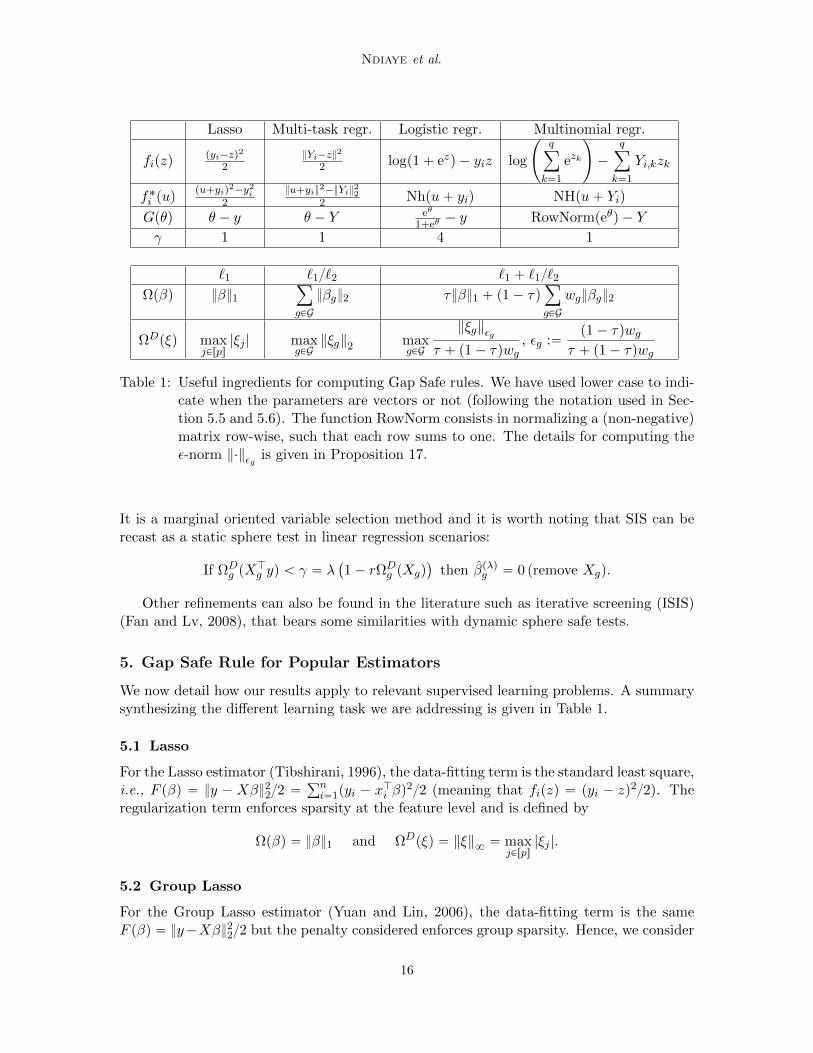
Table 1: Useful ingredients for computing Gap Safe rules. We have used lower case to indi-cate when the parameters are vectors or not (following the notation used in Sec-tion 5.5 and 5.6). The function RowNorm consists in normalizing a (non-negative)matrix row-wise, such that each row sums to one. The details for computing theε-norm ‖¨‖εg is given in Proposition 17.
It is a marginal oriented variable selection method and it is worth noting that SIS can berecast as a static sphere test in linear regression scenarios:
If ΩDg pX
Jg yq ă γ “ λ
`
1´ rΩDg pXgq
˘
then βpλqg “ 0 premove Xgq.
Other refinements can also be found in the literature such as iterative screening (ISIS)(Fan and Lv, 2008), that bears some similarities with dynamic sphere safe tests.
5. Gap Safe Rule for Popular Estimators
We now detail how our results apply to relevant supervised learning problems. A summarysynthesizing the different learning task we are addressing is given in Table 1.
5.1 Lasso
For the Lasso estimator (Tibshirani, 1996), the data-fitting term is the standard least square,i.e., F pβq “ y ´ Xβ222 “
řni“1pyi ´ xJi βq
22 (meaning that fipzq “ pyi ´ zq22). Theregularization term enforces sparsity at the feature level and is defined by
Ωpβq “ β1 and ΩDpξq “ ‖ξ‖8 “ maxjPrps
|ξj |.
5.2 Group Lasso
For the Group Lasso estimator (Yuan and Lin, 2006), the data-fitting term is the sameF pβq “ y´Xβ222 but the penalty considered enforces group sparsity. Hence, we consider
16

Gap Safe Screening Rules
the norm Ωpβq “ Ωwpβq, often referred to as an `1`2 norm, defined by:
Ωwpβq :“ÿ
gPGwg ‖βg‖2 and ΩD
w pξq :“ maxgPG
‖ξg‖2wg
,
where w “ pwgqgPG are some weights satisfying wg ą 0 for all g P G.
5.3 Sparse-Group Lasso
In the Sparse-Group Lasso case, we also have β P Rp and F pβq “ y ´ Xβ222 but theregularization Ωpβq “ Ωτ,wpβq is defined by
Ωτ,wpβq :“ τβ1 ` p1´ τqÿ
gPGwg ‖βg‖2 ,
for τ P r0, 1s, w “ pwgqgPG with wg ě 0 for all g P G. Note that we recover the Lasso ifτ “ 1, and the Group Lasso if τ “ 0; the case where wg “ 0 for some g P G together withτ “ 0 is excluded (Ωτ,w is not a norm in such a case). This estimator was introduced bySimon et al. (2013) to enforce sparsity both at the feature and at the group level, and wasused in different applications such as brain imaging in Gramfort et al. (2013) or in genomicsin Peng et al. (2010). Other hierarchical norms have also been proposed in Sprechmannet al. (2010) or Jenatton et al. (2011) and could be handled in our framework moduloadditional technical details.
For the Sparse-Group Lasso, the geometry of the dual feasible set ∆X is more complex(cf. Figure 3 for a comparison w.r.t. Lasso and Group Lasso). As a consequence, additionalgeometrical insights are needed to derive efficient safe rules, especially to compute the dualnorm required by Equation (9) and the computation of the safe screening rules given in (7).
We now introduce the ε-norm (denoted ‖¨‖ε) as it has a connection with the Sparse-Group Lasso norm Ωτ,w. The ε-norm was first proposed in Burdakov (1988) for otherpurposes (see also Burdakov and Merkulov (2001)). For any ε P r0, 1s and any x P Rd, ‖x‖εis defined as the unique nonnegative solution ν of the following equation (for ε “ 0, wedefine ‖x‖ε“0 :“ ‖x‖8):
dÿ
i“1
p|xi| ´ p1´ εqνq2` “ pενq
2. (17)
Using soft-thresholding, this is equivalent to solve in ν the equation ‖STp1´εqνpxq‖2 “ εν.Moreover, its dual norm is given by; see (Burdakov and Merkulov, 2001, Equation (42)):
‖ξ‖Dε “ ε‖ξ‖D2 ` p1´ εq‖ξ‖D8 “ ε‖ξ‖2 ` p1´ εq‖ξ‖1 . (18)
This allows to express the Sparse-Group Lasso norm Ωτ,w using the dual ε-norm. Wenow derive an explicit formulation for the dual norm of the Sparse-Group Lasso, originallyproposed in (Ndiaye et al., 2016b, Prop. 4):
17
Ndiaye et al.
Proposition 17 For all groups g in G, let us introduce εg :“p1´ τqwg
τ ` p1´ τqwg. Then, the
Sparse-Group Lasso norm satisfies the following properties: for any β and ξ in Rp,
Ωτ,wpβq “ÿ
gPGpτ ` p1´ τqwgqβg
Dεg and ΩD
τ,wpξq “ maxgPG
‖ξg‖εgτ ` p1´ τqwg
.
BΩDt,w“
ξ P Rp : @g P G, ‖STτ pξgq‖2 ď p1´ τqwg(
.
BΩτ,wpβq “ tz P Rp : @g P G, zg P τB‖¨‖1pβgq ` p1´ τqwgB‖¨‖2pβgqu .
Hence the dual feasible set is given by
∆X “
θ P Rn : @g P G, ‖STτ
`
XJg θ˘
‖2 ď p1´ τqwg(
“
θ P Rn : @g P G, ‖XJg θ‖εg ď τ ` p1´ τqwg(
.
Remark 18 Computing the dual norm of the Sparse-Group Lasso involves solving for eachgroup g P G, a problem similar to the one given in (17) which has a quadratic complexity.To overcome this difficulty, an efficient algorithm relying on sorting techniques was proposedin (Ndiaye et al., 2016b, Prop. 5) to perform exact dual norm evaluation.
The Sparse-Group Lasso benefits from two levels of screening: the safe rules can detectboth group-wise zeros and coordinate-wise zeros in the remaining groups: for any groupg in G and any safe sphere Bpθ, rq, Equation (7) and the sub-differential of the Sparse-Group Lasso norm in Proposition 17 give (a detailed proof is given in (Ndiaye et al., 2016b,Appendix C))
Group level safe screening rule: maxθPBpθ,rq
‖XJg θ‖εgτ ` p1´ τqwg
ă 1 ñ βpλqg “ 0.
Feature level safe screening rule: @j P g, maxθPBpθ,rq
|XJj θ| ă τ ñ βpλqj “ 0.
Noting that ‖STτ pxq‖2 “ p1´ τqwg ðñ ‖x‖εg “ τ `p1´ τqwg, the above screening teston the group level can be rewritten as
maxθPBpθ,rq
∥∥STτ pXJg θq
∥∥2ă p1´ τqwg ñ βpλqg “ 0.
The advantage of this formulation is that one can easily derive a “tight” upper-boundof the non-convex optimization problem in the left hand side of the preceding test. Indeed,we have STτ pxq “ x ´ ΠτB8pxq which brings us finally into a geometric problem easier tosolve. We recall from (Ndiaye et al., 2016b, Prop. 1) that for any center θ P ∆X , any groupg P G and any j P g, we have the following upper-bound
maxθPBpθ,rq
|XJj θ| ď |XJj θ| ` r ‖Xj‖2 ,
maxθPBpθ,rq
∥∥STτ pXJg θq
∥∥2ď Tg :“
#∥∥STτ pXJg θq
∥∥2` r ‖Xg‖2 , if
∥∥XJg θ∥∥8 ą τ,
p∥∥XJg θ∥∥8 ` r ‖Xg‖2 ´ τq`, otherwise.
Hence we derive the two level of safe screening rule:
18

Gap Safe Screening Rules
(a) Lasso dual ball BΩD forΩDpθq “ θ8.
(b) Group Lasso dual ball BΩD forΩDpθq “ maxp
a
θ21 ` θ
22, |θ3|q.
(c) Sparse-Group Lasso dual ballBΩD “
θ : @g P G, STτ pθgq2 ďp1´ τqwg
(
.
Figure 3: Lasso, Group Lasso and Sparse-Group Lasso dual unit balls: BΩD “ tθ : ΩDpθq ď1u. For the illustration, the group structure is chosen such that G “ tt1, 2u, t3uu,i.e., g1 “ t1, 2u, g2 “ t3u, n “ p “ 3, wg1 “ wg2 “ 1 and τ “ 12.
Proposition 19 (Safe screening rule for the Sparse-Group Lasso)
Group level screening: @g P G, if Tg ă p1´ τqwg, then βpλqg “ 0.
Feature level screening: @g P G,@j P g, if |XJj θ| ` r ‖Xj‖2 ă τ, then βpλqj “ 0.
In the same spirit than Proposition 14, for any safe region R, i.e., a set containing θpλq,we define two levels of active sets, one for the group level and one for the feature level:
AgppRq :“ tg P G, maxθPR
∥∥STτ pXJg θq
∥∥2ě p1´ τqwgu,
AftpRq :“ď
gPAgppRqtj P g : max
θPR|XJj θ| ě τu.
If one considers sequence of converging regions, then the next proposition (see (Ndiaye et al.,2016b, Prop. 3)) states that we can identify in finite time the optimal active sets definedas follows:
Egp :“!
g P G :∥∥∥STτ pX
Jg θpλqq
∥∥∥2“ p1´ τqwg
)
, Eft :“ď
gPEgp
!
j P g : |XJj θpλq| ě τ
)
.
Proposition 20 Let pRkqkPN be a sequence of safe regions whose diameters converge to 0.Then, lim
kÑ8AgppRkq “ Egp and lim
kÑ8AftpRkq “ Eft.
5.4 `1 Regularized Logistic Regression
Here, we consider the formulation given in (Buhlmann and van de Geer, 2011, Chapter 3)for the two-class logistic regression. In such a context, one observes for each i P rns a classlabel li P t1, 2u. This information can be recast as yi “ 1tli“1u (where 1 is the indicatorfunction), and it is then customary to minimize (3) where
F pβq “nÿ
i“1
`
´yixJi β ` log
`
1` exp`
xJi β˘˘˘
, (19)
19

Ndiaye et al.
with fipzq “ ´yiz ` logp1 ` exppzqq, and the penalty is simply the `1 norm: Ωpβq “ β1.Let us introduce Nh, the (binary) negative entropy function defined by:
Nhpxq “
#
x logpxq ` p1´ xq logp1´ xq, if x P r0, 1s ,
`8, otherwise .(20)
We use the convention 0 logp0q “ 0, and one can check that f˚i pziq “ Nhpzi` yiq and γ “ 4.
Remark 21 We have privileged the formulation with the label y P t0, 1un instead of y Pt`1,´1un in order to be consistent with the multinomial cases below. One can simply switchfrom one formulation to the other thanks to the mapping ry “ 2y ´ 1.
5.5 `1`2 Multi-task Regression
The multi-task Lasso is a regression problem where the parameters form a matrix B P Rpˆq.Denoting n the number of observations for each task k P rqs, it is defined as
minBPRpˆq
1
2‖Y ´XB‖2F ` λ
pÿ
j“1
‖Bj,:‖2 , (21)
where X P Rnˆp and Y P Rnˆq. Here we assume that the explanatory variables X areshared among the tasks however the Gap Safe rules would readily apply to the non-shareddesign formulation as in Lee et al. (2010) or in Liu et al. (2009) since the loss is still smooth(cf. Remark 7).
Introducing the vec operator that vectorizes a matrix by stacking its columns to forma column vector, and the Kronecker product b of two matrices, the multi-task Lasso canbe rewritten as a special case of Group Lasso. In fact, we have n class of observationsci “ pi ` pk ´ 1qnqkPrqs of size q for each i P rns (the overall number of observations isn1 “ nq) and p groups gj “ pj ` pk ´ 1qpqkPrqs such that |gj | “ q for j P rps. The
design matrix X “ Iq b X P Rn1ˆp1 “ Rnqˆpq is a q-block diagonal matrix defined asX “ diagpX, . . . ,Xq, y “ vecpY q and β “ vecpBq, we have:
minβPRp1
1
2
nÿ
i“1
∥∥yci ´ xJi β∥∥2
2` λ
pÿ
j“1
∥∥βgj∥∥2, (22)
i.e., fipzq “ ‖yci ´ z‖222. The advantage of this formulation is that it can be conciselywritten using the matrix forms of y and β, without the need to actually construct the largematrix X 1. This is particularly appealing for the implementation.
In signal processing, this model is also referred to as the Multiple Measurement Vector(MMV) problem. It allows to jointly select the same features for multiple regression tasks,see (Argyriou et al., 2006, 2008; Obozinski et al., 2010). This estimator has been usedin various applications such as prediction of the location of a protein within a cell (Xuet al., 2011) or in neuroscience (Gramfort et al., 2012), for instance to diagnose Alzheimer’sdisease (Zhang et al., 2012).
20
Gap Safe Screening Rules
5.6 `1`2 Multinomial Logistic Regression
We adapt the formulation given in (Buhlmann and van de Geer, 2011, Chapter 3) for themultinomial regression. In such a context, one observes for each i P rns a class label li P rqs.This information can be recast into a matrix Y P Rnˆq filled by 0’s and 1’s: Yi,k “ 1tli“ku(where 1 is the indicator function). In the same spirit as for the multi-task Lasso, a matrixB P Rpˆq is formed by q vectors encoding the hyperplanes for the linear classification. Thusthe multinomial `1`2 regularized regression reads:
minBPRpˆq
nÿ
i“1
˜
qÿ
k“1
´Yi,kxJi B:,k ` log
˜
qÿ
k“1
exp`
xJi B:,k
˘
¸¸
` λ
pÿ
j“1
‖Bj,:‖2 . (23)
Using a similar reformulation as in Section 5.5 i.e., defining ci “ pi`pk´ 1qnqkPrqs for eachi P rns and gj “ pj ` pk´ 1qpqkPrqs for each j P rps, the `1`2 multinomial logistic regressioncan be cast into our framework as:
minβPRp1
nÿ
i“1
fi`
xJi β˘
` λ
pÿ
j“1
∥∥βgj∥∥2, (24)
with fi : Rq Ñ R such that fipzq “ ´yJciz` log
`řqk“1 exp pzkq
˘
. Note that generalizing (3)to functions fi : Rq Ñ R does not bear difficulties, see Ndiaye et al. (2015).
Let us introduce NH, the negative entropy function defined by
NHpxq “
#
řqi“1 xi logpxiq, if x P Σq “ tx P Rq` :
řqi“1 xi “ 1u,
`8, otherwise.(25)
We use the convention 0 logp0q “ 0, and one can check that f˚i pzq “ NHpz` Yiq and γ “ 1.For multinomial logistic regression, Dλ implicitly encodes the additional constraint θ P
domDλ “ tθ1 P Rn : @i P rns,´λθ1ci ` yci P Σqu where Σq is the q dimensional simplex, see
Equation (25). By the dual scaling Equation (9), we have:
θ “ Θ
˜
´GpXβq
λ
¸
“R
maxpλ,ΩDpXJRqq, with R “ y ´ RowNormpexppXβqq
where the function RowNorm consists in normalizing a (non-negative) matrix row-wise, suchthat each row sums to one. Thus for any i P rns and α :“ λmaxpλ,ΩDpXJRqq P r0, 1s,
´λθci ` yci “ p1´ αqyci ` αRowNormpexppxJi βqq
which is a convex combination of elements in Σq. Hence the dual scaling (9) preserves thisadditional constraint.
Remark 22 The intercept has been neglected in our models for simplicity. The Gap Safeframework can also handle such a feature to the cost of more technical details (by adaptingthe results from Koh et al. (2007) for instance). However, in practice, the intercept can behandled in the present formulation by adding a constant column to the design matrix X.The intercept is then regularized. However, if the constant is set high enough, regularizationis small and experiments show that it has little to no impact for high-dimensional problems.This is the strategy used in the Liblinear package by Fan et al. (2008). Another alternativecould be to handle the constant term as is performed by El Ghaoui et al. (2012).
21

Ndiaye et al.
6. Experiments
In this section we present results obtained with the Gap Safe rules on various data sets.Implementation9 has been done in Python and Cython (Behnel et al., 2011) for low levelcritical parts. A coordinate descent algorithm is used with a scaled dual gap stoppingcriterion i.e., we normalize the targeted accuracy ε (in the stopping criterion) in order tohave a running time that is independent from the data scaling, i.e., ε Ð ε‖y‖22 for theregression cases and εÐ εminpn1, n2qn where ni is the number of observations in the classi, for the logistic cases.
Note that in the Lasso case, to compare our method with the un-safe strong rulesby Tibshirani et al. (2012) and with the sequential screening rule such as the eddp+ by Wanget al. (2012), we have added an approximated KKT post-processing step. We do thisfollowing Footnote 8, since they require the previous (exact) dual optimal solution which isnot available in practice (Ndiaye et al., 2016b, Appendix B). The same limit holds true forthe TLFre approach of Wang and Ye (2014) addressing the Sparse-Group Lasso formulation,as well as for the method explored by Lee and Xing (2014) to handle overlapping groupsand slores by Wang et al. (2014) for the binary logistic regression.
We have compared our method to various known safe screening rules (El Ghaoui et al.,2012; Xiang et al., 2011; Bonnefoy et al., 2014). For the Sparse-Group Lasso, such rulesdid not exist, so we have proposed natural extensions (Ndiaye et al., 2016b) thanks toexact computation of the dual norm in Proposition 17. For the Lasso estimator, we havealso compared our implementation with the Blitz algorithm (Johnson and Guestrin, 2015)which combines Gap Safe screening rules, Prox-Newton coordinate descent and an activeset strategy.
6.1 `1 Lasso Regression
Figure 4: Lasso on the Leukemia (dense data with n “ 72 observations and p “ 7129features). fraction of the variables that are active. Each line corresponds to afixed number of iterations for which the algorithm is run.
9. The source code can be found in https://github.com/EugeneNdiaye.
22

Gap Safe Screening Rules
(a) Dense grid with 100 values of λ.
(b) Coarse grid with 10 values of λ.
Figure 5: Lasso on the Leukemia (dense data with n “ 72 observations and p “ 7129features). Computation times needed to solve the Lasso regression path to desiredaccuracy for a grid of λ from λmax to λmax103.
We have evaluated the computing time for the Gap Safe rules with and without activewarm start, and compared with the static rule El Ghaoui et al. (2012) and the refineddynamic rule DST3 by Xiang et al. (2011), as well as Bonnefoy et al. (2015). We usedthe classic dense data set Leukemia, and the large sparse financial data set E2006-log1pavailable from LIBSVM10. We have normalized the column of X and standardized y tohave zero mean and unit variance.
The experiments on Figure 4 focuses on the Leukemia data set. The screening per-formance for a fixed number of iterations, from 2 to 29, is investigated for each λ. It
10. http://www.csie.ntu.edu.tw/~cjlin/libsvmtools/datasets/
23

Ndiaye et al.
demonstrates that increasing the number of iterations benefits to the dynamic screeningrule. Also, the closer the estimate is from the global minimum, the better the screening.This is inline with the results in running time in the benchmark on Figure 5(a). Note thatthe dynamic Gap Safe rule is the only rule that significantly improves the running time ofthe Lasso.
(a) Dense grid with 100 values of λ.
(b) Sparse grid with 10 values of λ.
Figure 6: Lasso on financial data E2006-log1p (sparse data with n “ 16087 observations andp “ 1668737 features). Computation times needed to solve the Lasso regressionpath to desired accuracy for a grid of λ from λmax to λmax20.
Results presented in the financial data set in Figure 6 are inline with the results onLeukemia. We observe that the Blitz algorithm (Johnson and Guestrin, 2015), also achievesa significant speed-up with gains in the same order of magnitude than our dynamic Gap Safe
24

Gap Safe Screening Rules
implementation combined with active or strong warm start. One advantage of our approachthough, is the simplicity to insert it in any iterative algorithm as shown in Algorithm 1 and 2.
To demonstrate the limitations of the strong rules, we report in Figure 5(b) resultswith a coarse grid with only 10 values of λ from λmax to λmax103 such that 2λt ă λt´1.The strong rules become then useless since the screening test (14) selects all variables,i.e., ST Gpθpλt´1q, λt, λt´1q “ G. Overall, the greater the gap between grid points, the lowerthe benefits of (active) warm start.
In the experiment in Figure 6(b), we have stopped the grid at λmax20 leading to asparse solution with 1562 active variables. We obtain an important speed-up for bothcoarse and dense grids demonstrating the consistent efficiency of the active warm startstrategy specially in a sparse regime.
Finally, with an extremely coarse grid, we therefore recommend the active warm startwith the previous safe active set (which performance is only affected through the initializa-tion point) rather than the strong active set (cf. Figure 5(b)).
6.2 `1 Binary Logistic Regression
Results on the Leukemia data set for standard logistic regression are reported in Figure 7.We compare the dynamic strategy of Gap Safe to the sequential strategy. Results demon-strate the clear benefit of the dynamic rule in terms of high number of screened out variables.This is reflected in the graph of running times, which shows that dynamic Gap Safe rulewith strong warm start can yield up to a 30ˆ speed-up compared to sequential rule andeven more compared to an absence of screening (up to 50ˆ speed-up).
6.3 `1`2 Multi-task Regression
To demonstrate the benefit of the Gap Safe screening rules for a multi-task Lasso problemwe have considered neuroimaging data. Electroencephalography (EEG) and magnetoen-cephalography (MEG) are brain imaging modalities that allow to identify active brain re-gions. The problem to solve is a multi-task regression problem with squared loss where everytask corresponds to a time instant. Using a multi-task Lasso one can constrain the recoveredsources to be identical during a short time interval (Gramfort et al., 2012). This correspondsto a temporal stationary assumption. In this experiment we used a joint MEG/EEG datawith 301 MEG and 59 EEG sensors leading to n “ 360. The number of possible sources isp “ 22, 494 and the number of time instants is q “ 20. With a 1 kHz sampling rate it isequivalent to say that the sources stay the same for 20 ms.
Results are presented in Figure 8. The Gap Safe rule is compared with the dynamicsafe rule from Bonnefoy et al. (2015). Figure 8(a) shows the fraction of active variables. Itdemonstrates that the Gap Safe rule screens out much more variables than the comparedmethods. Thanks to the converging nature of our rule, the more iterations are performedthe more variables are screened out. On Figure 8(b), the computation time confirms theeffective speed-up. Our rule significantly improves the computation time for all dualitygap tolerance from 10´2 to 10´8, especially when accurate estimates are required, e.g., forfeature selection.
25

Ndiaye et al.
(a) Fraction of the variables that are active. Each linecorresponds to a fixed number of iterations for whichthe algorithm is run.
(b) Computation times needed to solve the logistic regression path to desired accuracy with 100 values of λfrom λmax to λmax103.
Figure 7: `1 regularized binary logistic regression on the Leukemia (dense data with n “ 72observations and p “ 7129 features). Sequential and full dynamic screening GapSafe rules are compared.
6.4 Sparse-Group Lasso Regression
We consider the data set NCEP/NCAR Reanalysis 1 Kalnay et al. (1996) which containsmonthly means of climate data measurements spread across the globe in a grid of 2.5˝ˆ2.5˝
resolutions (longitude and latitude 144 ˆ 73) from 194811 to 20151031. Each gridpoint constitutes a group of 7 predictive variables (Air Temperature, Precipitable water,Relative humidity, Pressure, Sea Level Pressure, Horizontal Wind Speed and Vertical WindSpeed) whose concatenation across time constitutes our design matrix X P R814ˆ73577.Such data have therefore a natural group structure, with seven features per group. Astarget variable y P R814, we use the values of Air Temperature in a neighborhood of Dakar.
26

Gap Safe Screening Rules
(a) Fraction of active variables as a function of λ andthe number of iterations K. The Gap Safe strategyhas a much longer range of λ with (red) small activesets.
(b) Computation time to reach convergence using different screening strategies. We have run the algorithmwith 100 values of λ from λmax to λmax103.
Figure 8: Experiments on MEG/EEG brain imaging data set (dense data with n “ 360observations, p “ 22494 features and q “ 20 time instants).
For preprocessing, we remove the seasonality (we center the data month by month) and thetrend (we remove the linear trend obtained by least squares) present in the data set. Wethen standardize the data so that each feature has a variance of one. This preprocessing isusually done in climate analysis to prevent some bias in the regression estimates. Similardata have been used in the past by Chatterjee et al. (2012), demonstrating that the Sparse-Group Lasso estimator is well suited for prediction in such climatology applications. Indeed,thanks to the sparsity structure, the estimates delineate via their support some predictiveregions at the group level, as well as predictive feature via coordinate-wise screening.
27
Ndiaye et al.
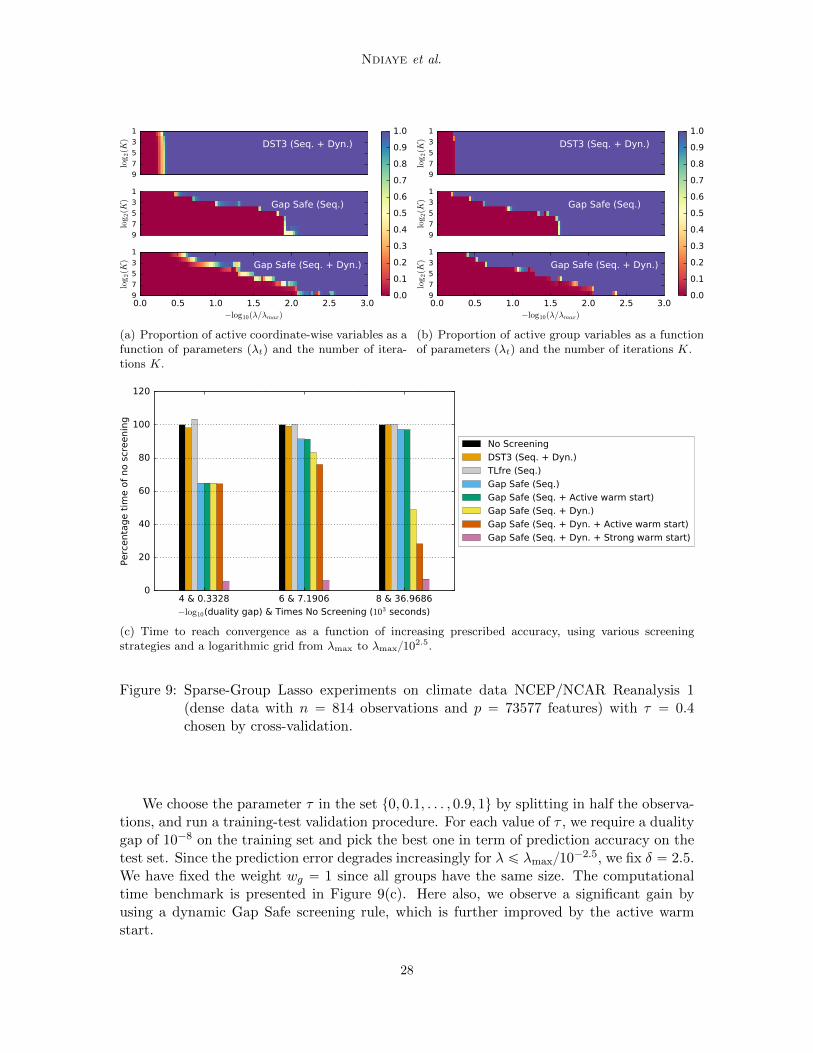
(a) Proportion of active coordinate-wise variables as afunction of parameters pλtq and the number of itera-tions K.
(b) Proportion of active group variables as a functionof parameters pλtq and the number of iterations K.
(c) Time to reach convergence as a function of increasing prescribed accuracy, using various screeningstrategies and a logarithmic grid from λmax to λmax102.5.
Figure 9: Sparse-Group Lasso experiments on climate data NCEP/NCAR Reanalysis 1(dense data with n “ 814 observations and p “ 73577 features) with τ “ 0.4chosen by cross-validation.
We choose the parameter τ in the set t0, 0.1, . . . , 0.9, 1u by splitting in half the observa-tions, and run a training-test validation procedure. For each value of τ , we require a dualitygap of 10´8 on the training set and pick the best one in term of prediction accuracy on thetest set. Since the prediction error degrades increasingly for λ ď λmax10´2.5, we fix δ “ 2.5.We have fixed the weight wg “ 1 since all groups have the same size. The computationaltime benchmark is presented in Figure 9(c). Here also, we observe a significant gain byusing a dynamic Gap Safe screening rule, which is further improved by the active warmstart.
28

Gap Safe Screening Rules
7. Conclusion
We have proposed a unified presentation of the Gap Safe screening rules for acceleratingalgorithms solving supervised learning problems under sparsity constraints. The proposedapproach applies to many popular estimators that boil down to convex optimization prob-lems where the data fitting term has a Lipschitz gradient and the regularization term is aseparable sparsity enforcing function. We have shown that our methodology is more flexiblethan previously known safe rules as it conveniently unifies both regression and classificationsettings. The efficiency of the Gap Safe rules along with the new active /strong warm startstrategies was demonstrated on multiple experiments using real high dimensional data set,suggesting that Gap Safe screening rules are always helpful to speed-up solvers targetingsparse regularization.
Acknowledgments
This work was supported by the ANR THALAMEEG ANR-14-NEUC-0002-01, the NIHR01 MH106174, by the ERC Starting Grant SLAB ERC-YStG-676943, by the Chair Ma-chine Learning for Big Data at Telecom ParisTech and by the Orange/Telecom ParisTechthink tank Phi-TAB. We would like to thank the reviewers for their valuable commentswhich contributed to improve the quality of this paper.
References
A. Argyriou, T. Evgeniou, and M. Pontil. Multi-task feature learning. In NIPS, pages41–48, 2006.
A. Argyriou, T. Evgeniou, and M. Pontil. Convex multi-task feature learning. MachineLearning, 73(3):243–272, 2008.
F. Bach, R. Jenatton, J. Mairal, and G. Obozinski. Convex optimization with sparsity-inducing norms. Foundations and Trends in Machine Learning, 4(1):1–106, 2012.
H. H. Bauschke and P. L. Combettes. Convex analysis and monotone operator theory inHilbert spaces. Springer, New York, 2011.
A. Beck and M. Teboulle. A fast iterative shrinkage-thresholding algorithm for linear inverseproblems. SIAM J. Imaging Sci., 2(1):183–202, 2009.
S. Behnel, R. Bradshaw, C. Citro, L. Dalcin, D.S. Seljebotn, and K. Smith. Cython: Thebest of both worlds. Computing in Science Engineering, 13(2):31 –39, 2011.
A. Bonnefoy, V. Emiya, L. Ralaivola, and R. Gribonval. A dynamic screening principle forthe lasso. In EUSIPCO, 2014.
A. Bonnefoy, V. Emiya, L. Ralaivola, and R. Gribonval. Dynamic Screening: AcceleratingFirst-Order Algorithms for the Lasso and Group-Lasso. IEEE Trans. Signal Process., 63(19):20, 2015.
29
Ndiaye et al.
S. Boyd, N. Parikh, E. Chu, B. Peleato, and J. Eckstein. Distributed optimization andstatistical learning via the alternating direction method of multipliers. Foundations andTrends in Machine Learning, 3(1):1–122, 2011.
P. Buhlmann and S. van de Geer. Statistics for high-dimensional data. Springer Series inStatistics. Springer, Heidelberg, 2011. Methods, theory and applications.
O. Burdakov. A new vector norm for nonlinear curve fitting and some other optimizationproblems. 33. Int. Wiss. Kolloq. Fortragsreihe ”Mathematische Optimierung — Theorieund Anwendungen”, pages 15–17, 1988.
O. Burdakov and B. Merkulov. On a new norm for data fitting and optimization problems.Linkoping University, Linkoping, Sweden, Tech. Rep. LiTH-MAT, 2001.
A. Chambolle and T. Pock. A first-order primal-dual algorithm for convex problems withapplications to imaging. J. Math. Imaging Vis., 40(1):120–145, 2011.
S. Chatterjee, K. Steinhaeuser, A. Banerjee, S. Chatterjee, and A. Ganguly. Sparse grouplasso: Consistency and climate applications. In SIAM International Conference on DataMining, pages 47–58, 2012.
B. Efron, T. Hastie, I. M. Johnstone, and R. Tibshirani. Least angle regression. Ann.Statist., 32(2):407–499, 2004. With discussion, and a rejoinder by the authors.
L. El Ghaoui, V. Viallon, and T. Rabbani. Safe feature elimination in sparse supervisedlearning. J. Pacific Optim., 8(4):667–698, 2012.
R.-E. Fan, K.-W. Chang, C.-J. Hsieh, X.-R. Wang, and C.-J. Lin. Liblinear: A library forlarge linear classification. J. Mach. Learn. Res., 9:1871–1874, 2008.
J. Fan and J. Lv. Sure independence screening for ultrahigh dimensional feature space. J.Roy. Statist. Soc. Ser. B, 70(5):849–911, 2008.
O. Fercoq, A. Gramfort, and J. Salmon. Mind the duality gap: safer rules for the lasso. InICML, pages 333–342, 2015.
J. Friedman, T. Hastie, H. Hofling, and R. Tibshirani. Pathwise coordinate optimization.Ann. Appl. Stat., 1(2):302–332, 2007.
J. Friedman, T. Hastie, and R. Tibshirani. Regularization paths for generalized linearmodels via coordinate descent. Journal of statistical software, 33(1):1, 2010.
W. J. Fu. Penalized regressions: the bridge versus the lasso. J. Comput. Graph. Statist., 7(3):397–416, 1998.
A. Gramfort, M. Kowalski, and M. Hamalainen. Mixed-norm estimates for the M/EEGinverse problem using accelerated gradient methods. Phys. Med. Biol., 57(7):1937–1961,2012.
30

Gap Safe Screening Rules
A. Gramfort, D. Strohmeier, J. Haueisen, M.S. Hmlinen, and M. Kowalski. Time-frequencymixed-norm estimates: Sparse M/EEG imaging with non-stationary source activations.NeuroImage, 70(0):410 – 422, 2013.
J.-B. Hiriart-Urruty and C. Lemarechal. Convex analysis and minimization algorithms. II,volume 306. Springer-Verlag, Berlin, 1993.
R. Jenatton, J. Mairal, G. Obozinski, and F. Bach. Proximal methods for hierarchicalsparse coding. J. Mach. Learn. Res., 12:2297–2334, 2011.
T. B. Johnson and C. Guestrin. Blitz: A principled meta-algorithm for scaling sparseoptimization. In ICML, pages 1171–1179, 2015.
T. B. Johnson and C. Guestrin. Unified methods for exploiting piecewise linear structurein convex optimization. In NIPS, pages 4754–4762, 2016.
E. Kalnay, M. Kanamitsu, R. Kistler, W. Collins, D. Deaven, L. Gandin, M. Iredell, S. Saha,G. White, J. Woollen, et al. The NCEP/NCAR 40-year reanalysis project. Bulletin ofthe American meteorological Society, 77(3):437–471, 1996.
K. Koh, S.-J. Kim, and S. Boyd. An interior-point method for large-scale l1-regularizedlogistic regression. J. Mach. Learn. Res., 8(8):1519–1555, 2007.
M. Kowalski, P. Weiss, A. Gramfort, and S. Anthoine. Accelerating ISTA with an activeset strategy. In OPT 2011: 4th International Workshop on Optimization for MachineLearning, page 7, 2011.
S. Lee and E. P. Xing. Screening rules for overlapping group lasso. preprintarXiv:1410.6880v1, 2014.
S. Lee, J. Zhu, and E. P. Xing. Adaptive multi-task lasso: with application to eqtl detection.In NIPS, pages 1306–1314, 2010.
J. Liang, J. Fadili, and G. Peyre. Local linear convergence of forward–backward underpartial smoothness. In NIPS, pages 1970–1978, 2014.
H. Liu, M. Palatucci, and J. Zhang. Blockwise coordinate descent procedures for the multi-task lasso, with applications to neural semantic basis discovery. In ICML, pages 649–656,2009.
E. Ndiaye, O. Fercoq, A. Gramfort, and J. Salmon. GAP safe screening rules for sparsemulti-task and multi-class models. NIPS, pages 811–819, 2015.
E. Ndiaye, O. Fercoq, A. Gramfort, V. Leclere, and J. Salmon. Efficient smoothed concomi-tant Lasso estimation for high dimensional regression. Arxiv preprint arXiv:1606.02702,2016a.
E. Ndiaye, O. Fercoq, A. Gramfort, and J. Salmon. GAP safe screening rules for Sparse-Group Lasso. NIPS, 2016b.
31

Ndiaye et al.
G. Obozinski, B. Taskar, and M. I. Jordan. Joint covariate selection and joint subspaceselection for multiple classification problems. Statistics and Computing, 20(2):231–252,2010.
J. Peng, J. Zhu, A. Bergamaschi, W. Han, D.-Y. Noh, J. R. Pollack, and P. Wang. Regu-larized multivariate regression for identifying master predictors with application to inte-grative genomics study of breast cancer. Ann. Appl. Stat., 4(1):53–77, 03 2010.
A. Raj, J. Olbrich, B. Gartner, B. Scholkopf, and M. Jaggi. Screening rules for convexproblems. arXiv preprint arXiv:1609.07478, 2016.
A. Shibagaki, M. Karasuyama, K. Hatano, and I. Takeuchi. Simultaneous safe screening offeatures and samples in doubly sparse modeling. In ICML, pages 1577–1586, 2016.
N. Simon, J. Friedman, T. Hastie, and R. Tibshirani. A sparse-group lasso. J. Comput.Graph. Statist., 22(2):231–245, 2013.
P. Sprechmann, I. Ramirez, G. Sapiro, and C. E. Yonina. Collaborative hierarchical sparsemodeling. In Information Sciences and Systems (CISS), 2010 44th Annual Conferenceon, pages 1–6. IEEE, 2010.
R. Tibshirani. Regression shrinkage and selection via the lasso. J. Roy. Statist. Soc. Ser.B, 58(1):267–288, 1996.
R. Tibshirani, J. Bien, J. Friedman, T. Hastie, N. Simon, J. Taylor, and R. J. Tibshirani.Strong rules for discarding predictors in lasso-type problems. J. Roy. Statist. Soc. Ser.B, 74(2):245–266, 2012.
R. J. Tibshirani. The lasso problem and uniqueness. Electron. J. Stat., 7:1456–1490, 2013.
J. Wang and J. Ye. Two-layer feature reduction for sparse-group lasso via decompositionof convex sets. arXiv preprint arXiv:1410.4210, 2014.
J. Wang, P. Wonka, and J. Ye. Lasso screening rules via dual polytope projection. arXivpreprint arXiv:1211.3966, 2012.
J. Wang, J. Zhou, J. Liu, P. Wonka, and J. Ye. A safe screening rule for sparse logisticregression. In NIPS, pages 1053–1061, 2014.
Z. J. Xiang, H. Xu, and P. J. Ramadge. Learning sparse representations of high dimensionaldata on large scale dictionaries. In NIPS, pages 900–908, 2011.
Z. J. Xiang, Y. Wang, and P. J. Ramadge. Screening tests for lasso problems. arXiv preprintarXiv:1405.4897, 2014.
Q. Xu, S. J. Pan, H. Xue, and Q. Yang. Multitask learning for protein subcellular locationprediction. IEEE/ACM Trans. Comput. Biol. Bioinformatics, 8(3):748–759, 2011.
M. Yuan and Y. Lin. Model selection and estimation in regression with grouped variables.J. Roy. Statist. Soc. Ser. B, 68(1):49–67, 2006.
32

Gap Safe Screening Rules
Y. Zeng and P. Breheny. The biglasso package: A memory- and computation-efficient solverfor lasso model fitting with big data in r. arXiv preprint arXiv:1701.05936, 2017.
D. Zhang, D. Shen, and Alzheimer’s Disease Neuroimaging Initiative. Multi-modal multi-task learning for joint prediction of multiple regression and classification variables inalzheimer’s disease. Neuroimage, 59(2):895–907, 2012.
J. Zimmert, C. S. de Witt, G. Kerg, and M. Kloft. Safe screening for support vectormachines. In NIPS 2015 Workshop on Optimization in Machine Learning (OPT), 2015.
33