f -GANs in an Information Geometric Nutshell

Richard Nock†,‡,§ Zac Cranko‡,† Aditya Krishna Menon†,‡

Lizhen Qu†,‡ Robert C. Williamson‡,†

†Data61, ‡the Australian National University and §the University of Sydneyfirstname.lastname, aditya.menon, bob.williamson@data61.csiro.au

Abstract

Nowozin et al showed last year how to extend the GAN principle to all f -divergences.The approach is elegant but falls short of a full description of the supervised game, andsays little about the key player, the generator: for example, what does the generatoractually converge to if solving the GAN game means convergence in some space ofparameters? How does that provide hints on the generator’s design and compare to theflourishing but almost exclusively experimental literature on the subject?

In this paper, we unveil a broad class of distributions for which such convergencehappens — namely, deformed exponential families, a wide superset of exponentialfamilies — and show tight connections with the three other key GAN parameters: loss,game and architecture. In particular, we show that current deep architectures are able tofactorize a very large number of such densities using an especially compact design, hencedisplaying the power of deep architectures and their concinnity in the f -GAN game.This result holds given a sufficient condition on activation functions — which turns outto be satisfied by popular choices. The key to our results is a variational generalizationof an old theorem that relates the KL divergence between regular exponential familiesand divergences between their natural parameters. We complete this picture withadditional results and experimental insights on how these results may be used to groundfurther improvements of GAN architectures, via (i) a principled design of the activationfunctions in the generator and (ii) an explicit integration of proper composite losses’link function in the discriminator.

1

arX

iv:1

707.

0438

5v1

[cs

.LG

] 1

4 Ju

l 201

7

1 IntroductionIn a recent paper, Nowozin et al. [47] showed that the GAN principle [27] can be extendedto the variational formulation of all f -divergences. In the GAN game, there is an unknowndistribution P which we want to approximate using a parameterized distribution Q. Q islearned by a generator by finding a saddle point of a function which we summarize for nowas f -GAN(P, Q), where f is a convex function (see eq. (14) below for its formal expression).A part of the generator’s training involves as a subroutine a supervised adversary — hence,the saddle point formulation – called discriminator, which tries to guess whether randomlygenerated observations come from P or Q. Ideally, at the end of this supervised game, wewant Q to be close to P, and a good measure of this is the f -divergence If (P‖Q), also knownas Ali-Silvey distance [1, 20]. Initially, one choice of f was considered [27]. Nowozin et al.significantly grounded the game and expanded its scope by showing that for any f convexand suitably defined, it actually holds that [47, Eq. 4]:

f -GAN(P, Q) ≤ If (P‖Q) . (1)

Furthermore, the inequality is an equality if the discriminator is powerful enough: so, solvingthe f -GAN game can give guarantees on how P and Q are distant to each other in terms off -divergence. This elegant characterization of the supervised game unfortunately falls shortof justifying or elucidating all parameters of the supervised game [47, Section 2.4].

The paper is also silent regarding a key part of the game: the link between distributions inthe variational formulation and the generator, the main player which learns a parametric modelof a density. In doing so, the f -GAN approach and its members remain within an informationtheoretic framework that relies on divergences between distributions only [47]. In the GANworld at large, this position contrasts with other prominent approaches that explicitly optimizegeometric distortions between the parameters or support of distributions [36]: momentmatching methods optimize distortions between expected parameters [35], Wasserstein-1method and optimal transport methods (regularized or not) optimize transportation costsbetween supports [7, 28, 24]. This problem of connecting the information theoretic and(information) geometric understanding of GANs is not just a theoretical question: there isgrowing experimental evidence that a careful geometric optimization, either on the support ofthe distributions [7, 28] or directly on these parameters [55] (which is related to the f -GANframework) improves further GANs.

So, how can we link the f -GAN approach to any sort of information geometric optimization?The variational formulation of the GAN game in eq. (1) hints on a specific direction ofresearch to answer this question: the identity between information-theoretic distortions ondistributions and information-geometric distortions on their parameterization [5]. One suchidentity is well known: The Kullback-Leibler (KL) divergence between two distributions ofthe same (regular) exponential family equals a Bregman divergence D between their naturalparameters [2, 5, 10, 14, 56], which we can summarize for now (the complete statement is inTheorem 2 below) as:

Ifkl(P‖Q) = D(θ‖ϑ) . (2)

Here, θ and ϑ are respectively the natural parameters of P and Q. Hence, distributions arerepresented by points on a manifold on the right-hand side, which is a powerful geometric

2

statement [5]; however, being restricted to KL divergence or "just" exponential families, itcertainly falls short of the power to explain the GAN game. To our knowledge, there is nopreviously known "GAN-amenable" generalization of this identity above exponential families.Related identities have recently been proven for two generalizations of exponential families[6, Theorem 9], [23, Theorem 3], but fall short of the f -divergence formulation and are notamenable to the variational GAN formulation.

Our first contribution is such an identity that connects the general If -divergence formula-tion in eq. (1) to the general D (Bregman) divergence formulation in eq. (2). We now brieflystate it, postponing the details to Section 3:

f -GAN(P, escort(Q)) = D(θ‖ϑ) + Penalty(Q) , (3)

for P and Q (with respective parameters θ and ϑ) which happen to lie in a superset of expo-nential families called deformed exponential families, that have received extensive treatmentin statistical physics and differential information geometry over the last decade [3, 41]. Theright-hand side of eq. (3) is the information geometric part [5], in which D is a Bregmandivergence. Therefore, whenever the Penalty is small, solving the f -GAN game solves ageometric optimization problem [5], like for the Wasserstein GAN and its variants [7], butwith the difference that the geometric part is essentially implicit. Notice also that Q appearsin the game in the form of an escort : its density is obtained from Q’s density through amapping (in general non-linear) completed with a simple normalization [6]. These differencesvanish only for exponential families: the mapping is the identity and thus escort(Q) = Q; also,Penalty(Q) = 0 and f = KL. This raises questions as to how eq. (3) and these differencesrelate to GAN architectures and the common understanding and implementation of thegeneral (f -)GAN game [27, 47].

Our second contribution answers several of these questions via several independent results.A subset is relevant to the f -GAN game at large:

(a) we completely specify the parameters of the supervised game, unveiling a key parameterleft arbitrary in [47] (explicitly incorporating the link function of proper compositelosses [53]);

(b) we develop a novel min-max game interpretation of eq. (3) in the context of the expectedutility theory [13];

(c) we show that relevant choices for escorts yield explicit upper bounds on the Penaltywhich vanish with the normalization coefficient of the escort.

Another subset dwells on deep architectures:

(d) we show that typical deep generator architectures are indeed powerful at modellingcomplex escorts of any deformed exponential family, factorising a number of escortsin order of the total inner layers’ dimensions; this provides theoretical support for thewidespread empirical speculations that deep architectures may be powerful at modelinghighly multimodal densities, which is a hot topic in the field [9];

3

(e) we show that this factorisation happens on an especially compact model design, com-pared e.g. to shallow architectures;

(f) we derive a connection between the parameters of the deformed exponential familiesand those of the generator. Quite notably, the activation function gives the deformedexponential family.

The connection between the generator and escorts via eq. (3) supports the use of geometricparameter based optimisation in the GAN game [55]. It suggests the existence of a large classof activation functions for which the factorisation in deformed exponential families holds asdescribed in (d-f). In a field where such functions have been the subject of intensive research[19, 37, 39] and face numerous constraints in their design [7, 49], the study of this class isnot just important for the theory at hand: it is also of high practical relevance.

Our last contribution studies this class and details several theoretical and experimentalfindings. We show that a simple sufficient condition on the activation function guaranteesthe escort modelling in (d), (f). Such a condition still allows for properties in activationthat handle sparsity, gradient vanishing, gradient exploding and/or Lipschitz continuity[7, 25, 49]. In fact, this condition is satisfied, exactly or in a limit sense, by most popularactivation functions (ELU, ReLU, Softplus, ...). We also provide experiments that display theuplift that can be obtained through tuning the activations (generator), or the link function(discriminator).The rest of this paper is as follows. Section § 2 presents definition, § 3 formally presents eq.(3), § 4 completes the supervised game picture of [47], § 5 derives a number of consequencesfor deep learning, including distributions achieved by deep architectures for the generator.Section § 6 presents experiments and a last Section concludes. An appendix contains allproofs and complementary experiments. Since our paper drills down into the four componentsof the GAN game (loss, distribution, game and architectures = models), we summarizefor clarity in appendix (Section 8) our main notations, the objects they refer to and theirrelationships through some of our key results.

Code availability — the code used for our experiments is available through

https://github.com/qulizhen/fgan_info_geometric

2 DefinitionsThroughout this paper, the domain X of observations is a measurable set. We begin withtwo important classes of distortion measures, f -divergences and Bregman divergences.

Definition 1 For any two distributions P and Q having respective densities P and Q abso-lutely continuous with respect to a base measure µ, the f -divergence between P and Q, wheref : R+ → R is convex with f(1) = 0, is

If (P‖Q).

= EX∼Q

[f

(P (X)

Q(X)

)]=

∫X

Q(x) · f(P (x)

Q(x)

)dµ(x) . (4)

4

For any convex differentiable ϕ : Rd → R, the (ϕ-)Bregman divergence between θ and % is:

Dϕ(θ‖%).

= ϕ(θ)− ϕ(%)− (θ − %)>∇ϕ(%) , (5)

where ϕ is called the generator of the Bregman divergence.

f -divergences are the key distortion measure of information theory. Under mild assumptions,they are the only distortions that satisfy the data processing inequality [30, 48]. Bregmandivergences are the key distortion measure of information geometry. Under mild assumptions,they are the only distortions that elicitate the sample average as a population minimizer[5, 11, 46, 58].

A distribution P from a (regular) exponential family with cumulant C : Θ → R andsufficient statistics φ : X→ Rd has density

PC(x|θ,φ).

= exp(φ(x)>θ − C(θ)) , (6)

where Θ is a convex open set, C is convex and ensures normalization on the simplex (weleave implicit the associated dominating measure [3]). A fundamental Theorem ties Bregmandivergences and f -divergences.

Theorem 2 [3, 14] Suppose P and Q belong to the same exponential family, and denotetheir respective densities PC(x|θ,φ) and QC(x|ϑ,φ). Then,

Ikl(P‖Q) = DC(ϑ‖θ) . (7)

Here, Ikl is Kullback-Leibler (KL) f -divergence (f .= x 7→ x log x).

Remark that the arguments in the Bregman divergence are permuted with respect tothose in eq. (2) in the introduction. This also holds if we consider fkl in eq. (2) tobe the Csiszár dual of f in Theorem 2 [13], namely fkl : x 7→ − log x, since in this caseIfkl(P‖Q) = Ikl(Q‖P) = DC(θ‖ϑ). We made this choice in the introduction for the sake ofreadability in presenting eqs. (1 — 3). Theorem 2 is useful because it shows that distributionscan be replaced by their parameterisation (and vice versa) to tackle a problem — we justneed to pick the right distortion for the objects at hand. There is analytic convenience inthis: for example, the Bregman divergence bypasses sampling issues to estimate the integralin the f -divergence — at the expense of the estimation of the parameters, though. In fact,Theorem 2 is so important that we state and prove a generalization of it in appendix, Section9, showing that dropping the "same family" constraint does not change the f -divergence(information-theoretic) vs Bregman divergence (information-geometric) picture.

We now define generalizations of exponential families, following [6, 23]. Let χ : R+ → R+

be non-decreasing [41, Chapter 10]. We define the χ-logarithm, logχ, as

logχ(z).

=

∫ z

1

1

χ(t)dt . (8)

The χ-exponential is

expχ(z).

= 1 +

∫ z

0

λ(t)dt , (9)

where λ is defined by λ(logχ(z)).

= χ(z). In the case where the integrals are improper, weconsider the corresponding limit in the argument / integrand.

5

Definition 3 [6] A distribution P from a χ-exponential family (or deformed exponentialfamily, χ being implicit) with convex cumulant C : Θ→ R and sufficient statistics φ : X→ Rd

has density given by:

Pχ,C(x|θ,φ).

= expχ(φ(x)>θ − C(θ)) , (10)

with respect to a dominating measure µ. Here, Θ is a convex open set and θ is called thecoordinate of P. The escort density (or χ-escort) of Pχ,C is

Pχ,C.

=1

Z· χ(Pχ,C) , (11)

where

Z.

=

∫X

χ(Pχ,C(x|θ,φ))dµ(x) (12)

is the escort’s normalization constant.

We leaving implicit the dominating measure and denote P the escort distribution of P whosedensity is given by eq. (11). We shall name χ the signature of the deformed (or χ-)exponentialfamily, and sometimes drop indexes to save readability without ambiguity, noting e.g. P forPχ,C . Notice that normalization in the escort is ensured by a simple integration [6, Eq. 7].For the escort to exist, we require that Z <∞ and therefore χ(P ) is finite almost everywhere.Such a requirement would naturally be satisfied in the GAN game.

There is another generalization of regular exponential families, known as generalizedexponential families [23] (appendix, Section 9). Their densities are defined from the subdiffer-ential of a convex function, but involves an inner product similar to eq. (10). There is noknown strict equivalent of Theorem 2 for whichever of the generalizations. For example, [23,Theorem 3] provides a generalization of Theorem 2 but replaces KL by a Bregman divergence1.The closest result appears for deformed exponential families [6, Theorem 9][59].

Theorem 4 [6][59] for any two χ-exponential distributions P and Q with respective densitiesPχ,C , Qχ,C and coordinates θ, ϑ,

DC(θ‖ϑ) = EX∼Q[logχ(Qχ,C(X))− logχ(Pχ,C(X))] . (13)

Theorem 4 is a generalization of Theorem 2 for χ(z).

= z, in which case logχ = log, expχ = exp

and escorts disappear: Q = Q. There are two important things to notice in eq. (13):

• the expectation is computed over the escort of Q;

• the difference of two χ-logarithms is in general not the χ-logarithm of the density ratio.

The f -GAN game relies on distortions being formulated via convex functions over densityratios. As such, Theorem 4 is not amenable to the variational f -GAN formulation [47, Section2.2]. In the following Section, we show how to achieve this goal, but before, we briefly framethe now popular (f -)GAN adversarial learning [27, 47].

1Under mild assumptions on support and functions, KL = f -divergences ∩ Bregman divergences [30].

6

We have a true unknown distribution P over a set of objects, e.g. 3D pictures, whichwe want to learn. In the GAN setting, this is the objective of a generator, who learns adistribution Qθ parameterized by vector θ. Qθ works by passing (the support of) a simple,uninformed distribution, e.g. standard Gaussian, through a possibly complex function, e.g. adeep net whose parameters are θ and maps to the support of the objects of interest. FittingQ. involves an adversary (the discriminator) as subroutine, which fits classifiers, e.g. deepnets, parameterized by ω. The generator’s objective is to come up with arg minθ Lf (θ) withLf (θ) the discriminator’s objective:

Lf (θ).

= supωEX∼P[Tω(X)]− EX∼Qθ [f

?(Tω(X))] , (14)

where ? is Legendre conjugate [15] and Tω : X→ R integrates the classifier of the discriminatorand is therefore parameterized by ω. Lf is a variational approximation to a f -divergence[47]; the discriminator’s objective is to segregate true (P) from fake (Q.) data. The originalGAN choice, [27]

fgan(z).

= z log z − (z + 1) log(z + 1) + 2 log 2 (15)

(the constant ensures f(1) = 0) can be replaced by any convex f meeting mild assumptions.

3 A variational information geometric identity for the f-GAN game

We now make a series of Lemmata and Theorems that will bring us to formalize eq. (3),in two main steps: first, we show that the right-hand side of eq. (13) in Theorem 4 can bereformulated using a new set of distortion measures which is amenable to the variationalf -GAN formulation. Second, we connect this variational formulation to the classical f -GANgame [47] by showing that, modulo finiteness conditions that make sense to the GAN game,this new set of distortion measures essentially coincides with f -divergences.

KLχ divergences — First, we define this new set of distortion measures, that we call KLχdivergences.

Definition 5 For any χ-logarithm and distributions P,Q having respective densities P andQ absolutely continuous with respect to base measure µ, the KLχ divergence between P andQ is defined as:

KLχ(P‖Q).

= EX∼P

[− logχ

(Q(X)

P (X)

)]. (16)

Since χ is non-decreasing, − logχ is convex and so any KLχ divergence is an f -divergence.When χ(z)

.= z, KLχ is the KL divergence. In what follows, base measure µ and absolute

continuity are implicit, as well as that P (resp. Q) is the density of P (resp. Q). In the sameway as f divergences are invariant to specific affine translations (see the proof of Theorem 7),KLχ divergences satisfy an interesting invariance.

7

Lemma 6 For any χ-logarithm, distributions P,Q and constant k ∈ R+,

KLχ(P‖Q).

= KL χ1+kχ

(P‖Q) . (17)

(Proof in appendix, Section 10) Hence, we can in fact assume that any KLχ divergence isobtained for a signature which is bounded.

KLχ divergences vs f-divergences — Let ∂f be the subdifferential of convex f andIP,Q

.= [infx P (x)/Q(x), supx P (x)/Q(x)) ⊆ R+ denote the range of density ratios of P

over Q. Our first result states that if there is an element of the subdifferential which isupperbounded on IP,Q, the f -divergence If (P‖Q) is equal to a KLχ divergence.

Theorem 7 Suppose that P,Q are such that ∃ξ ∈ ∂f with sup ξ(IP,Q) < ∞. Then ∃χ :R+ → R+ non decreasing such that If (P‖Q) = KLχ(Q‖P).

Remark. Notice that because the constraint relies on the subdifferential, it actually doesnot prevent the f -divergence to diverge. Also, Theorem 7 essentially covers most if not allrelevant GAN cases, as the assumption has to be satisfied in the GAN game for its solutionnot to be vacuous up to a large extent (eq. (14)). Indeed, if the subdifferential diverges on afinite ratio, then the optimal ω makes Tω explode on some x [47, Eq. 5]. If it diverges on aninfinite ratio, then lim+∞ f(z) = +∞ and essentially If (P‖Q) is unbounded. In this case, Qvanishes in the neighborhood of some x ∈ X for which P > 0. We can make Lf (θ) artificiallylarge by just picking ω such that Tω is as large as necessary in such a neighborhood: thediscriminator only focuses on one "pit" of Q (relative to P ) to detect natural examples, whichis not an appealing solution to the GAN game.The proof of Theorem 7 (in appendix, Section 11) is constructive: it shows how to pick χwhich satisfies all requirements. It brings the following interesting corollary: under mildassumptions on f , there exists a χ that fits for all densities P and Q. A prominent exampleof f that fits is the original GAN choice for which we can pick

χgan(z).

=1

log(1 + 1

z

) . (18)

Corollary 8 Suppose ∃ξ ∈ ∂f with sup ξ(intdomf) < ∞. Then ∃χ : R+ → R+ increasingsuch that for any distributions P, Q, If (P‖Q) = KLχ(Q‖P).

Remark. Even when f does not satisfy Corollary 8, it may well be the case that its Csiszárdual does [13], or equivalently, that Corollary 8 holds if we permute the arguments in one ofthe distortions. Let f(z)

.= z · f(1/z). We have If(P‖Q) = If(Q‖P). Then, for example,

picking f(z) = z log z (KL) does not fit to Corollary 8 but picking f(z) = − log z (reverseKL) does. Picking Pearson χ2 (f(z) = (z − 1)2) does not fit to Corollary 8 but pickingf(z) = (1/z) · (z − 1)2 (Neyman χ2) does.We now show that when the subdifferential diverges (but If is finite), it it still possible toapproximate If (P‖Q) by some KLχ divergence, up to any required precision.

8

Theorem 9 Suppose that P,Q are such that sup ξ(IP,Q) = +∞, ∀ξ ∈ ∂f , but If (P‖Q) < +∞,then ∀δ > 0, ∃χ : R+ → R+ increasing such that

KLχ(Q‖P) ≤ If (P‖Q) ≤ KLχ(Q‖P) + δ . (19)

(Proof in appendix, Section 12)

A KLχ divergences formulation for Theorem 4 — To connect KLχ-divergences andTheorem 4, we need a slight generalization of KLχ-divergences and allow for χ in eq. (16) todepend on the choice of the expectation’s X, granted that for any of these choices, it will meetthe constraints to be R+ → R+ and also increasing, and therefore define a valid signature.For any f : X→ R+, we denote

KLχf (P‖Q).

= EX∼P

[− logχf(X)

(Q(X)

P (X)

)], (20)

where for any p ∈ R+,

χp(t).

=1

p· χ(tp) . (21)

Whenever f = 1, we just write KLχ as we already did in Definition 5. We note that forany x ∈ X, χf(x) is increasing and non negative because of the properties of χ and f , soχf(x)(t) defines a χ-logarithm. We also note that the invariance of Lemma 6 holds as wellfor KLχf (P‖Q). With this generalization of KLχ, we are ready to state a Theorem thatconnects KLχ-divergences and Theorem 4.

Theorem 10 Letting P .= Pχ,C and Q .

= Qχ,C for short in Theorem 4, we have:

EX∼Q[logχ(Q(X))− logχ(P (X))] = KLχQ(Q‖P)− J(Q) , (22)

with

J(Q).

= KLχQ(Q‖Q) . (23)

(Proof in appendix, Section 13) To summarize, we know that under mild assumptions rel-atively to the GAN game, f -divergences coincide with KLχ divergences (Theorems 7, 9).We also know from Theorem 10 that KLχ. divergences quantify the geometric proximitybetween the coordinates of generalized exponential families (Theorem 4). Hence, finding ageometric (parameter-based) interpretation of the variational f -GAN game as described in eq.(14) can be done via a variational formulation of theKLχ divergences appearing in Theorem 10.

A variational formulation for KLχ divergences — Since penalty J(Q) does not belongto the GAN game (it does not depend on P), it reduces our focus on KLχQ(Q‖P).

Theorem 11 KLχQ(Q‖P ) admits the variational formulation

KLχQ(Q‖P) = supT∈R++

X

EX∼P[T (X)]− EX∼Q[(− logχQ)?(T (X))]

, (24)

9

with R++.

= R\R++. Furthermore, letting Z denoting the normalization constant of theχ-escort of Q, the optimum T ∗ : X→ R++ to eq. (24) is

T ∗(x) = − 1

Z· χ(Q(x))

χ(P (x)). (25)

(Proof in appendix, Section 14) Hence, the variational f -GAN formulation can be capturedin an information-geometric framework by the following identity using Theorems 4, 7, 10, 11.

Corollary 12 (the variational information-geometric f-GAN identity) Using notationsfrom Theorems 10, 11, we have

supT∈R++

X

EX∼P[T (X)]− EX∼Q[(− logχQ)?(T (X))]

= DC(θ‖ϑ) + J(Q) , (26)

where θ (resp. ϑ) is the coordinate of P (resp. Q).

We shall also name for short vig-f -GAN the identity in eq. (26). Even when it is not neededto understand the high-level picture of the identity, we can reduce the Legendre conjugate(− logχQ)? to an equivalent "dual" (negative) χ•-logarithm in the variational problem.

Theorem 13 The variational formulation of KLχQ(Q‖P) (Theorem 11) satisfies:

supT∈R++

X

EX∼P[T (X)]− EX∼Q[(− logχQ)?(T (X))]

= sup

T∈R++X

EX∼P[T (X)]− EX∼Q

[− log(χ•) 1

Q

(−T (X))

]−K(Q) , (27)

where K(.) is a function of Q only and

χ•(t).

=1

χ−1(

1t

) . (28)

(Proof in appendix, Section 15) Since only the "sup" part is of interest in the superviseddiscriminator-generator game, the main interest of Theorem 13 is to give a more preciseshape to the losses involved in the supervised game (See Section 4).Remark. The left hand-side of Eq. (26) has the exact same overall shape as the variationalobjective of [47, Eqs 2, 6], in which we would have equivalently f = − logχQ , f

? = − log(χ•)1/Q,

eq. (14). However, it tells the formal story of GANs in significantly greater details, in particularfor what concerns the generator. For example, eq. (26) yields a new characterization of thegenerators’ convergence: because DC is a Bregman divergence, it satisfies the identity ofthe indiscernibles. So, up to the proximity of Q to its escort (to have J(Q) small), solvingthe f -GAN game [47] guarantees convergence in the parameter space (ϑ vs θ). In therealm of GAN applications, it makes sense to consider that P (the true distribution) can beextremely complex. Therefore, even when deformed exponential families are significantly moreexpressive than regular exponential families [41], extra care should be put before arguing that

10

complex applications comply with such a geometric convergence in the parameter space. Oneway to circumvent this problem is to build distributions in Q that factorize many deformedexponential families. This is one strong point of deep architectures that we shall prove inSection 5.

We also remark two key component of the vig-f -GAN identify in deformed exponentialfamilies which are absent from Theorem 2:

(1) the generator (Q) appears in the form of an escort in the variational component — thisdistinction vanishes for exponential families, where Q = Q;

(2) an information theoretic penalty appears in the identity (J(Q)) — this penalty vanishesfor exponential families, for which J(Q) = 0.

These two components are crucial to link the f -GAN variational optimization to the geometricconvergence in the parameter space. We shall drill down into both in Section 5.

4 A complete proper loss picture of the supervised GANgame

In their generalization of the GAN objective, Nowozin et al. [47] leave untold a key partof the supervised game: they split in eq. (14) the discriminator’s contribution in two,Tω = gf Vω, where Vω : X→ R is the actual discriminator, and gf is essentially a technicalconstraint to ensure that Vω(.) is in the domain of f ?. They leave the choice of gf "some-what arbitrary" [47, Section 2.4]. We now show that if one wants the supervised loss tohave the desirable property to be proper composite [53]2, then gf is not arbitrary. We pro-ceed in three steps, first unveiling a broad class of proper f -GANs that deal with this property.

Proper f-GANs — The initial motivation of eq. (14) was that the inner maximisationmay be seen as the f -divergence between P and Qθ [42], Lf(θ) = If(P‖Qθ). In fact, thisvariational representation of an f -divergence holds more generally: by [54, Theorem 9], weknow that for any convex f , and invertible link function Ψ: (0, 1)→ R, we have:

infT : X→R

E(X,Y)∼D

[`Ψ(Y, T (X))] = −1

2· If (P ‖Q) (29)

where D is the distribution over (observations × fake, real) and the loss function `Ψ isdefined by:

`Ψ(+1, z).

= −f ′(

Ψ−1(z)

1−Ψ−1(z)

); `Ψ(−1, z)

.= f ?

(f ′(

Ψ−1(z)

1−Ψ−1(z)

)), (30)

assuming f differentiable. Note now that picking Ψ(z) = f ′(z/(1− z)) with z .= T (x) and

simplifying eq. (29) with P[Y = fake] = P[Y = real] = 1/2 in the GAN game yields eq. (14).For other link functions, however, we get an equally valid class of losses whose optimisation

2informally, Bayes rule realizes the optimum and the loss accommodates for any real valued predictor.

11

will yield a meaningful estimate of the f -divergence. The losses of eq. (30) belong to theclass of proper composite losses with link function Ψ [53]. Thus (omitting parameters θ,ω),we rephrase eq. (14) and refer to the proper f -GAN formulation as infQ LΨ(Q) with (` is asper eq. (30)):

LΨ(Q).

= supT : X→R

E

X∼P[−`Ψ(+1, T (X))] + E

X∼Q[−`Ψ(−1, T (X))]

. (31)

Note also that it is trivial to start from a suitable proper composite loss, and derive thecorresponding generator f for the f -divergence as per eq. (29). Finally, our proper compositeloss view of the f -GAN game allows us to elicitate gf in [47]: it is the composition of f ′ andΨ in eq. (30).

Proper f-GANs and density ratios — The use of proper composite losses as part of thesupervised GAN formulation sheds further light on another aspect the game: the connectionbetween the value of the optimal discriminator, and the density ratio between the generator anddiscriminator distributions. Instead of the optimal T ∗(x) = f ′(P (x)/Q(x)) for eq. (14) [47,Eq. 5], we now have with the more general eq. (31) the result T ∗(x) = Ψ((1+Q(x)/P (x))−1).

Proper vig-f-GANs — We now show that proper f -GANs can easily be adapted to eq.(26).

Theorem 14 For any χ, define `x(−1, z).

= − log(χ•) 1Q(x)

(−z), and let `(+1, z).

= −z. Then

LΨ(Q) in eq. (31) equals eq. (26). Its link in eq. (31) is

Ψx(z) = − 1

χQ(x)

(z

1−z

) . (32)

(Proof in appendix, Section 16) Hence, in the proper composite view of the vig-f -GANidentity, the generator rules over the supervised game: it tempers with both the link functionand the loss — but only for fake examples. Notice also that when z = −1, the fake examplesloss satisfies `x(−1,−1) = 0 regardless of x by definition of the χ-logarithm.

5 Consequences for deep learningIn this Section, we highlight a number of consequences of our results, from the standpoint ofdeep learning. Eq. (26) shows the importance for the generator to be able to model escorts— and complex ones, in the realm of the GAN applications. We start here with a proofthat, when used for the generator, mainstream deep architectures [34] are amenable to suchcomplex factorizations of escorts using an especially compact design.

5.1 Deep architectures and escorts in the vig-f-GAN game

In the GAN game, distribution Q in eq. (26) is built by the generator (call it Qg), by passingthe support of a simple distribution (e.g. uniform, standard Gaussian), Qin, through a series

12

Qin

L1,d

L1,1

L1,2

1,1

1,2

1,d

2,1

2,2

2,d

L,1

L,2

L,d

x1

x2

xd

in deep out

gd

g1

g2w1, b1 w2, b2 wL, bL ,

v v v vout

Qg

Figure 1: Deep architecture for the generator; it takes as input a simple distribution (Qin)and outputs a complex distribution (Qg) through a (deep) series of non-linear transformations(best viewed in color, see text).

of non-linear transformations (Figure 1). Letting Qin denote the corresponding density, wenow compute Qg. Our generator g : X→ Rd consists of two parts: a deep part and a lastlayer. The deep part is, given some L ∈ N, the computation of a non-linear transformationφL : X→ RdL as

Rdl 3 φl(x).

= v(wlφl−1(x) + bl) , ∀l ∈ 1, 2, ..., L , (33)φ0(x)

.= x ∈ X . (34)

v is a function computed coordinate-wise, such as (leaky) ReLUs, ELUs [19, 29, 37, 39],wl ∈ Rdl×dl−1 , bl ∈ Rdl . The last layer computes the generator’s output from φL:

g(x).

= vout(ΓφL(x) + β) , (35)

with Γ ∈ Rd×dL ,β ∈ Rd; in general, vout 6= v and vout fits the output to the domain at hand,ranging from linear [7, 34] to non-linear functions like tanh [47]. Our generator, sketchedin Figure 1 captures the high-level features of some state of the art generative approaches[52, 60, 62].

To carry our analysis, we make the assumption that the network is reversible, which isgoing to reguire that vout,Γ,wl (l ∈ 1, 2, ..., L) are invertible. Since vout would be in manyexperimental cases (identity, tanh, etc.), we essentially assume that dimensions match like inFigure 1 and so the simple input density is in fact of dimension d (e.g. uniform over X = ahypercube). At this reasonable price, we get in closed form the generator’s density and itshows the following: for any continuous signature χnet, there exists an activation functionv such that the deep, most important part in the network (Figure 1) can factor exactly asescorts for the χnet-exponential family. Let 1i denote the ith canonical basis vector.

Theorem 15 ∀vout,Γ,wl invertible (l ∈ 1, 2, ..., L), for any continuous signature χnet,there exists activation v and bl ∈ Rd (∀l ∈ 1, 2, ..., L) such that for any output z, letting

13

x.

= g−1(z), Qg(z) factorizes as:

Qg(z) =Qin(x)

Qdeep(x)· 1

Hout(x) · Znet

, (36)

with Znet > 0 a constant, Hout(x).

=∏d

i=1 |v′out(γ>i φL(x) + βi)|, γi .= Γ>1i, and (letting

wl,i.

= w>l 1i):

Qdeep(x).

=L∏l=1

d∏i=1

Pχnet,bl,i(x|wl,i,φl−1) . (37)

(Proof in appendix, Section 17) The relationship between the inner layers of a deep net anddeformed exponential families (Definition 3) follows from the Theorem:

• rows in wls define coordinates;

• φl define "deep" sufficient statistics;

• bl are cumulants;

• the crucial part, the χ-family, is given by the activation function v.

Notice also that the bls are learned, and so the deformed exponential families’ normalizationis in fact learned and not specified. The proof of the Theorem comments on a simplificationof the constant when we also suppose that the escorts’ normalization is not specified. Theproof of the Theorem also comments on two additional keypoints:

(i) how Qg(z) may factor as a likelihood on a graphical model defined by the inner layersof g;

(ii) how the "twist" introduced by Hout(x) can be absorbed in a "det(.)" volume elementwith general sigmoid activations [47, 60, 52, 62], which is standard to the changeof variable formula [21]. We also note that with linear activation [7, 34], Hout(x) isconstant.

We see that Qdeep factors escorts, and in number, which is good news with respect to thepower of deep architectures and their adequation to the GAN framework. What is remarkableis the compactness achieved by the deep representation: the total dimension of all deepsufficient statistics in Qdeep (eq. (37)) is L ·d. To handle this, a shallow net with a single innerlayer would require a matrix w of space Ω(L2 · d2). The deep net g requires only O(L · d2)space to store all wls.

5.2 Escort-compliant design of inner activations in the generator

The proof of Theorem 15 is constructive: it builds v as a function of χ. In fact, the proofalso shows how to build χ from the activation function v in such a way that Qdeep factorsχ-escorts. The following Lemma essentially says that this is possible for all strongly admissibleactivations v.

14

χ

0 1

2 3

4 5

z 0

1

µ 0

1

Figure 2: Convergence of the signature χ for µ-ReLU to that of ReLU (dashed pink at theback, also displayed in Figure 3).

Definition 16 Activation function v is strongly admissible iff dom(v)∩R+ 6= ∅ and v is C1,lowerbounded, strictly increasing and convex.

Lemma 17 For any strongly admissible v, there exists signature χ such that Theorem 15holds.

(proof in appendix, Section 18) (γ,γ)-ELU (for any γ > 0), Softplus are strongly admissible,which leaves open the status of more general ELUs, leaky ReLU and, or course, ReLU[19, 22, 37, 39]. We note that these latter activations satisfy parts of the constraints already,as they are increasing, convex and meet the domain requirement. We shall analyze themthrough the property that they can be arbitrarily closely approximated by a strongly admissibleactivation, a property that we define as weak admissibility.

Definition 18 Activation v is weakly admissible iff for any ε > 0, there exists vε stronglyadmissible such that ||v − vε||L1 < ε, where ||f ||L1

.=∫|f(t)|dt.

Notice that the constraint is stronger than just controlling supz |v(z)− vε(z)|. Nevertheless,we can prove the following.

Lemma 19 ReLU is weakly admissible.

(proof in appendix, Section 19) The trick is simple: approximate the function by a stronglyadmissible smooth activation, to get rid of the fact that ReLU is not differentiable everywhereand not strictly increasing. For this reason, this trick can easily be repeated for (α, β)-ELU.For leaky-ReLU, we need to add the constraint that the domain is lowerbounded, and then

15

Name v(z) χ(z)

ReLU(§) max0, z 1z>0

Leaky-ReLU(†)

z if z > 0εz if z ≤ 0

1 if z > −δ1ε

if z ≤ −δ(α, β)-ELU(♥)

βz if z > 0

α(exp(z)− 1) if z ≤ 0

β if z > αz if z ≤ α

prop-τ (♣) k + τ?(z)τ?(0)

τ ′−1(τ?)−1(τ?(0)z)τ?(0)

Softplus(♦) k + log2(1 + exp(z)) 1log 2· (1− 2−z)

µ-ReLU(♠) k +z+√

(1−µ)2+z2

24z2

(1−µ)2+4z2

LSU(¶) k +

0 if z < −1

(1 + z)2 if z ∈ [−1, 1]4z if z > 1

2√z if z < 4

4 if z > 4

Table 1: Some (strongly or weakly) admissible couples (v, χ). (§) : 1. is the indicator function;(†) : δ ≤ 0, 0 < ε ≤ 1 and dom(v) = [δ/ε,+∞). (♥) : β ≥ α > 0; (♣) : ? is Legendreconjugate; (♠) : µ ∈ [0, 1). Shaded: prop-τ activations; k is a constant (e.g. such thatv(0) = 0); (¶) : LSU = Least Square Unit (see text).

the trick is the same. Table 1 presents several couples (v, χ) for which v is (strongly orweakly) admissible. In the case where v is strongly admissible, we give the signature χ thatwould be obtained through Lemma 17. If it is weakly admissible, we give the limit χ forthe sequence of strong admissible activations in Definition 18. Figure 2 gives an example ofsuch a sequence for the µ-ReLU activation. Table 1 includes a wide class of so-called "prop-τactivations", where τ is negative a concave entropy, defined on [0, 1] and symmetric around1/2 [45]. Softplus [22] is a prop-τ activation. We also remark that ReLU = limµ→1 µ-ReLU (inthe sense that limµ→1 supz |ReLU(z)− µ-ReLU(z)| = 0). One property of prop-τ activationsis especially handy for Wasserstein GANs [7, Eq. 3]: prop-τ activations are Lipschitz (proof in[44, Section 3]). Finally, the LSU activation should in theory be constrained to domain [−1, 1],so we have linearly extended it to R by linearity, keeping convexity and differentiability.Figure 3 plots several choices of signatures χ, corresponding to different choices of activationfunctions, distributions or f -divergences (Figure 9 in appendix provides the correspondencefrom the choice of χ).

5.3 J(Q) vs not J(Q)

By focusing on the left hand side of eq. (26), the usual f -GAN approaches [47] guaranteeconvergence in the parameter spaces which is all the better as J(Q) is small after convergence.This is happening when χ is (close enough to) identity because in this case Q→ Q, but this isnot really interesting in the context of deep learning where non-linear transformations implyχ is not going to comply (Theorem 15). For several interesting cases, we show an upperboundon J(Q) which is decreasing with Z, the normalization parameter of the escort (Definition 3).Recall that J(Q)

.= KLχQ(Q‖Q), so there needs to be two components to specify J : χ and

16

0

1

2

3

4

5

6

0 1 2 3 4 5

exp. fam.

LSU

(2,2.5)-ELU(1,2)-ELU

Softplus

GAN

ReLU

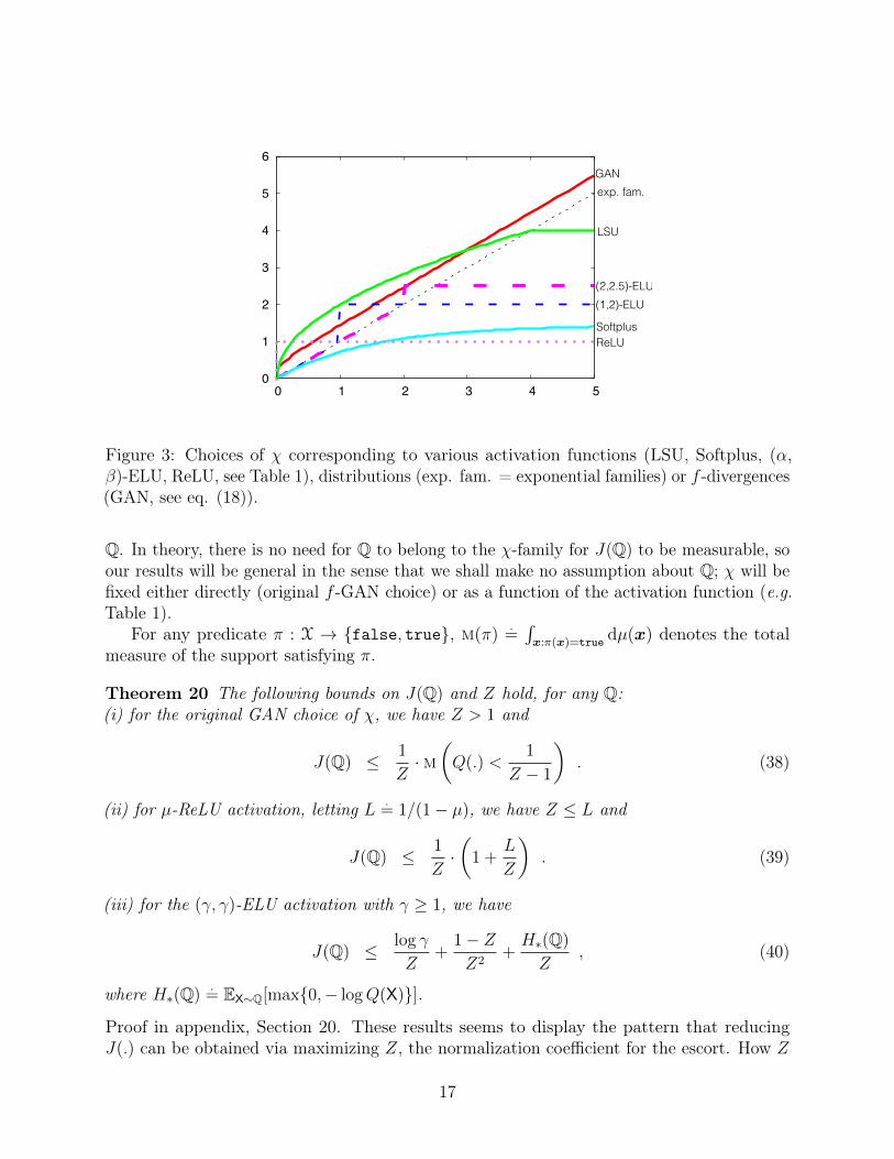
Figure 3: Choices of χ corresponding to various activation functions (LSU, Softplus, (α,β)-ELU, ReLU, see Table 1), distributions (exp. fam. = exponential families) or f -divergences(GAN, see eq. (18)).

Q. In theory, there is no need for Q to belong to the χ-family for J(Q) to be measurable, soour results will be general in the sense that we shall make no assumption about Q; χ will befixed either directly (original f -GAN choice) or as a function of the activation function (e.g.Table 1).

For any predicate π : X → false, true, m(π).

=∫x:π(x)=true dµ(x) denotes the total

measure of the support satisfying π.

Theorem 20 The following bounds on J(Q) and Z hold, for any Q:(i) for the original GAN choice of χ, we have Z > 1 and

J(Q) ≤ 1

Z·m(Q(.) <

1

Z − 1

). (38)

(ii) for µ-ReLU activation, letting L .= 1/(1− µ), we have Z ≤ L and

J(Q) ≤ 1

Z·(

1 +L

Z

). (39)

(iii) for the (γ, γ)-ELU activation with γ ≥ 1, we have

J(Q) ≤ log γ

Z+

1− ZZ2

+H∗(Q)

Z, (40)

where H∗(Q).

= EX∼Q[max0,− logQ(X)].Proof in appendix, Section 20. These results seems to display the pattern that reducingJ(.) can be obtained via maximizing Z, the normalization coefficient for the escort. How Z

17

Figure 4: Illustration of the effect of passing a density (upper-left) through some signature χ(black curves), without normalization.

0

0.2

0.4

0.6

0.8

1

1.2

1.4

1.6

1.8

2

-4 -3 -2 -1 0 1 2 3 4 5

µ = 0.01, δ = 0µ = 0.99, δ = 0

µ = 0.01, δ = 0.35

Figure 5: Escorts of a standard Gaussian (dashed), for a leaky-χδ,ε (see text).

depends in fine on χ, v is non trivial. It seems that picking χ that augments the "contrast"(blows up high density regions) is a good idea. Figure 4 presents some examples of densityshapes (not normalized) obtained from a simple density passed through various χ, showinghow one can control such a contrast. Figure 5 does the same for a standard Gaussian, wherethe resulting densities (in color) are normalized. Since Lemma 17 is very general, we canengineer very specific χs for this objective: inspired from the leaky-ReLU activation, theexample of Figure 5 uses such leaky-χ escorts when χ is that of the µ-ReLU (Table 1, δ > 0,small ε > 0):

χδ,ε(z).

= 1z<δ · (εz) + 1z≥δ · (εδ + χ(z − δ)) . (41)

5.4 How to play the proper-GAN game

In [50], the density ratio connection was used to modify the GAN training procedure asfollows: first, one trains the discriminator to solve the inner maximisation in eq. (14) forconvex f ; next, one estimates the density ratio r(x) = P (x)/Q(x) by

r(x) = (f ′)−1(T ∗(x)) , (42)

finally, one trains the generator to minimise the f -divergence Iϕ(P‖Q) = EX′∼Qϕ(r(X′)) forconvex ϕ. In terms of proper composite losses, the first two steps can be generalised as

18

follows: first, one trains the discriminator to solve the inner maximisation in eq. (31) forconvex f and link function Ψ; next, one estimates the density ratio r(x) = P (x)/Q(x) byr(x) = Ψ−1(T ∗(x))/(1−Ψ−1(T ∗(x))). Note that this allows us e.g. to use the logistic loss,for which Ψ(z) = log(z/(1− z)) and f(z) = z · log z − (z + 1) · log(z + 1) + 2 log 2 = fgan(z)(eq. (15)).

5.5 A more complete picture of geometric optimization in GANs

Any Bregman divergence is locally Mahalanobis’, i.e. a squared distance with a particularmetric [5, Section 3]. For eq. (26), is means when C is strictly convex that ∀θP ,ϑQ, thereexists Symmetric Positive Definite (SPD) matrix m such that

DC(θP‖ϑQ) = DC?(µQ‖µP ) = ‖µQ − µP‖2m , (43)

where µ..

= ∇C(θ.) = E.[φ] [12, Section 4]. Inner layers in the generator’s deep net aresufficient statistics (φ, Theorem 15 and Subsection 5.1). We see that the parameterizationchosen for the geometric optimization of [55, Section 3] looks like such a divergence, withm = i. The only difference with the vig-f -GAN identity is that the optimization occurs onthe statistics µQ,µP of the discriminator and not the generator, but it turns out that thef -divergences involved in the supervised game (Section 4 and [54]) also admit a formulationin terms of Bregman divergences [45] and therefore can be approximated using eq. (43).Hence, our results support the feature matching technique of Salimans et al. [55, Section 3.1].

5.6 The generator can accomodate complex multimodal densities

This is currently a hot topic in GAN architectures, with some concerns raised about thecapacity of the networks to capture multimodal densities [8, 9]. More specifically, wheneverthe discriminator is too "small", then the generator may be trapped in densities with verysmall support, thereby preventing it to capture the many modes of highly multi-modaldensities. This is the so-called "mode collapse" problem, and it is crucial since the modes ofa density being its local maxima, they locally represent the most natural objects to model.Because GAN applications are complex, one works with the objective to capture numerousmodes [17]. We consider the problem from the generator’s side and ask, at first hand, whetherit is amenable to model such complex densities — if it were not, then GAN architectureswould be doomed beyond the training concerns raised by [8, 9].

Such a question can be answered in the affirmative via Theorem 15 (See appendix, Section21), yet it requires specific signatures tailor made for the generator’s density to captureall modes. It is therefore more a theoretical result than a proof of validity for currentarchitectures, yet using such signatures can accomodate as many as Ω(d · L) modes.

5.7 Playing the (vig-)f-GAN game in the expected utility theory

To play the GAN game at its fullest extent, we need to understand it in extenso. Most ofthe game-theoretic focus on GANs has been focused on the convergence and/or its Nashequilibrium [8, 26], around the idea that the generator tries to "fool" the discriminator. The

19

expected utility theory allows to better qualify the quotes directly in the context of thevig-f -GAN game. This requires some background which we now briefly state [16].

In an insurance market, a portfolio is a function Υ : X→ R such that Υ(x) is the amountof cash Υ pays to whomever holds it under the state of the world x ∈ X (negative payoffs areinterpreted as costs to the asset holder). Portfolio management for a Decision Maker (DM)works in two steps: first, DM purchases the portfolio Υ with market prices P , for a costκ

.= EX∼P [Υ(X)]. Then DM receives a payoff Υ(x) upon the revelation of the state of the

world x ∈ X. In the expected utility theory [16], assuming DM (i) has a quasilinear utilityfunction and (ii) maximises expected utility according to subjective beliefs Q. Then thereexists utility udm : R → R increasing and concave such that DM achieves maximal utilityU(Q):

U(Q).

= supΥ:X→R

EX∼Q

[udm(Υ(X))− κ

]= sup

Υ:X→REX∼P[−Υ(X)] + EX∼Q[udm(Υ(X))] .(44)

Suppose now that subjective beliefs Q are in the hand of another player, G, distinct fromDM, and whose objective is to minimize U(Q), the game being the horizon of of min-maxoptimization iterations. The following Lemma sheds light on the key parameters of the game.

Lemma 21 The DM vs G game is equivalent to the (vig-)f -GAN game (eq. (26)) in whichDM = discriminator, G = generator, the set of portfolios Υ = T, the subjective beliefsQ = Q and the utility

udm(z) = log(χ•) 1Q

(z) . (45)

(Proof in appendix, Section 22) Hence, G tampers with the utility function of DM in thisgame — which, we note, amounts for G to learn the true market prices P . There is more todrill from the game in terms of risk aversion, as shown below.

Lemma 22 Let the Arrow-Pratt coefficient of absolute risk aversion [51] aux(z).

= −u′′(z)u′(z)

,and the Arrow-Pratt coefficient of relative risk aversion, ru(z)

.= z · au(z). Suppose χ

differentiable. Then, in the DM vs G game, (i) DM is always risk averse. Furthermore, (ii)ru(z) is also indexed by X ∼ Q and we have

rux(z) = g

(z

Q(x)

), (46)

g(z).

= z · (χ−1)′(z)

χ−1(z). (47)

Finally, (iii) at the optimum Υ∗, we have

rux(Υ∗(x)) = g

(1

χ(P (x))

). (48)

(Proof in appendix, Section 23) Hence, DM is always risk averse and his relative risk aversiondepends on subjective beliefs with the notable exception of the optimum T ∗ for which itdepends on market prices only. Everything is like if DM was getting rid of G’s influencedsubjective beliefs to come up with the optimal solution.

20

µ

Figure 6: Summary of our results on MNIST, on experiment A, comparing different values ofµ for the µ-ReLU activation in the generator (ReLU = 1-ReLU, see text). Thicker horizontaldashed lines present the ReLU average baseline: for each color, points above the baselinesrepresent values of µ for which ReLU is beaten on average.

6 ExperimentsTwo of our theoretical contributions are:

(A) the fact that on the generator ’s side, there exists numerous activation functions v thatcomply with the design of its density as factoring escorts (Lemma 17), and

(B) the fact that on the discriminator ’s side, the so-called output activation function gf of[47] aggregates in fact two components of proper composite losses, one of which, thelink function Ψ, should be a fine knob to operate (Theorem 14).

We have tested these two possibilities with the idea that an experimental validation shouldprovide substantial ground to be competitive with mainstream approaches, leaving space fora finer tuning in specific applications. Also, in order not to mix their effects, we have treated(A) and (B) separately.

Architectures and datasets — We provide in appendix (Section 23) the detail of allexperiments. To summarize, we consider two architectures in our experiments: DCGAN [52]and the multilayer feedforward network (MLP) used in [47]. Our datasets are MNIST [33]and LSUN tower category [61].

Comparison of varying activations in the generator (A) — We have compared µ-ReLUs with varying µ in [0, 0.1, ..., 1] (hence, we include ReLU as a baseline for µ = 1), theSoftplus and the LSU activation (Figure 1). For each choice of the activation function, all

21

SoftplusLSUReLU

Figure 7: Summary of our results on MNIST, on experiment A, comparing different activationsin the generator, for the same architectures as in Figure 6.

inner layers of the generator use the same activation function. We evaluate the activationfunctions by using both DCGAN and the MLP used in [47] as the architectures. As trainingdivergence, we adopt both GAN [27] and Wasserstein GAN (WGAN, [7]). Results are shownin Figure 6. Three behaviours emerge when varying µ: either it is globally equivalent to ReLU(GAN DCGAN) but with local variations that can be better (µ = 0.7) or worse (µ = 0), orit is almost consistently better than ReLU (WGAN MLP) or worse (GAN MLP). The bestresults were obtained for GAN DCGAN, and we note that the ReLU baseline was essentiallybeaten for values of µ yielding smaller variance, and hence yielding smaller uncertainty inthe results.

The comparison between different activation functions (Figure 7) reveals that (µ-)ReLUperforms overall the best, yet with some variations among architectures. We note in particularthat, in the same way as for the comparisons intra µ-ReLU (Figure 6), ReLU performs rela-tively worse than the other criteria for WGAN MLP, indicating that there may be differentbest fit activations for different architectures, which is good news. Visual results on LSUN(appendix, Table 7) also display the quality of results when changing the µ-ReLU activation.

Comparison of varying link functions in the discriminator (B) — We have comparedthe replacement of the sigmoid function by a link which corresponds to the entropy whichis theoretically optimal in boosting algorithms, Matsushita entropy [31, 44], for whichΨmat(z)

.= (1/2) · (1 + z/

√1 + z2) and the entropy (Table 1) is −τmat(z) = 2

√z(1− z).

Figure 8 displays the comparison Matsushita vs "standard" (more specifically, we use sigmoidin the case of GAN [47], and none in the case of WGAN to follow current implementations[7]). We evaluate with both DCGAN and MLP on MNIST (same hyperparameters as forgenerators, ReLU activation for all hidden layer activation of generators). Experiments tend

22

Figure 8: Summary of our results on MNIST, on experiment B, varying the link function inthe discriminator (see text).

to display that tuning the link may indeed bring additional uplift: for GANs, Matsushitais indeed better than the sigmoid link for both DCGAN and MLP, while it remains verycompetitive with the no-link (or equivalently an identity link) of WGAN, at least for DCGAN.

7 ConclusionIt is hard to exaggerate the success of GAN approaches in modelling complex domains, andwith their success comes an increasing need for a rigorous theoretical understanding [55].In this paper, we complete the supervised understanding of the generalization of GANsintroduced in [47], and provide a theoretical background to understand its unsupervised part.We show in particular how deep architectures can be powerful at tackling the generative partof the game, and can factor densities known to be far more general than exponential families,both in terms of the available densities (e.g. Cauchy, Student) or physical phenomena thatcan be modeled [6, 40, 41]. Our contribution therefore improves the understanding of bothplayers in the GAN game. Experiments display that the tools we develop may help to improvefurther the state of the art. Among the most prominent avenues for future work relies theintegration of penalty J(Q) directly in the GAN game. It turns out that a recent paper hasprecisely displayed that the introduction of a mutual information regularizer in the GANgame improves results and helps in disentangling representations [18].

8 AcknowledgmentsThe authors wish to thank Shun-ichi Amari, Giorgio Patrini and Frank Nielsen for numerouscomments.

23

References[1] S.-M. Ali and S.-D.-S. Silvey. A general class of coefficients of divergence of one

distribution from another. Journal of the Royal Statistical Society B, 28:131–142, 1966.

[2] S.-I. Amari. Differential-Geometrical Methods in Statistics. Springer-Verlag, Berlin,1985.

[3] S.-I. Amari. Information Geometry and Its Applications. Springer-Verlag, Berlin, 2016.

[4] S.-I. Amari. Personnal communication, 2017.

[5] S.-I. Amari and H. Nagaoka. Methods of Information Geometry. Oxford UniversityPress, 2000.

[6] S.-I. Amari, A. Ohara, and H. Matsuzoe. Geometry of deformed exponential families:Invariant, dually-flat and conformal geometries. Physica A: Statistical Mechanics andits Applications, 391:4308–4319, 2012.

[7] M. Arjovsky, S. Chintala, and L. Bottou. Wasserstein GAN. CoRR, abs/1701.07875,2017.

[8] S. Arora, R. Ge, Y. Liang, T. Ma, and Y. Zhang. Generalization and equilibrium ingenerative adversarial nets (GANs). CoRR, abs/1703.00573, 2017.

[9] S. Arora and Y. Zhang. Do GANs actually learn the distribution? an empirical study.CoRR, abs/1706.08224, 2017.

[10] K. S. Azoury and M. K. Warmuth. Relative loss bounds for on-line density estimationwith the exponential family of distributions. MLJ, 43(3):211–246, 2001.

[11] A. Banerjee, X. Guo, and H. Wang. On the optimality of conditional expectation as abregman predictor. IEEE Trans. IT, 51:2664–2669, 2005.

[12] A. Banerjee, S. Merugu, I. Dhillon, and J. Ghosh. Clustering with Bregman divergences.JMLR, 6:1705–1749, 2005.

[13] A. Ben-Tal, A. Ben-Israel, and M. Teboulle. Certainty equivalents and informationmeasures: Duality and extremal principles. J. of Math. Anal. Appl., pages 211–236,1991.

[14] J.-D. Boissonnat, F. Nielsen, and R. Nock. Bregman voronoi diagrams. DCG, 44(2):281–307, 2010.

[15] S. Boyd and L. Vandenberghe. Convex optimization. Cambridge University Press, 2004.

[16] J.-P. Chavas. Risk analysis in theory and practice. Academic press advanced finance,2004.

24

[17] T. Che, Y. Li, A.-P. Jacob, Y. Bengio, and W. Li. Mode regularized generative adversarialnetworks. In 5th ICLR, 2017.

[18] X. Chen, Y. Duan, R. Houthooft, J. Schulman, I. Sutskever, and P. Abbeel. InfoGAN:Interpretable representation learning by information maximizing generative adversarialnets. In NIPS*29, pages 2172–2180, 2016.

[19] D.-A. Clevert, T. Unterthiner, and S. Hochreiter. Fast and accurate deep networklearning by exponential linear units (ELUs). In 4th ICLR, 2016.

[20] I. Csiszár. Information-type measures of difference of probability distributions andindirect observation. Studia Scientiarum Mathematicarum Hungarica, 2:299–318, 1967.

[21] L. Dinh, J. Sohl-Dickstein, and S. Bengio. Density estimation using real NVP. In 5thICLR, 2017.

[22] C. Dugas, Y. Bengio, F. Bélisle, C. Nadeau, and R. Garcia. Incorporating second-orderfunctional knowledge for better option pricing. In Advances in Neural InformationProcessing Systems*13, pages 472–478, 2000.

[23] R.-M. Frongillo and M.-D. Reid. Convex foundations for generalized maxent models. In33rd MaxEnt, pages 11–16, 2014.

[24] A. Genevay, G. Peyré, and M. Cuturi. Sinkhorn-autodiff: Tractable Wasserstein learningof generative models. CoRR, abs/1706.00292, 2017.

[25] X. Glorot, A. Bordes, and Y. Bengio. Deep sparse rectifier neural networks. In 14thAISTATS, pages 315–323, 2011.

[26] I. Goodfellow. Generative adversarial networks, 2016. NIPS’16 tutorials.

[27] I. Goodfellow, J. Pouget-Abadie, M. Mirza, B. Xu, D. Warde-Farley, S. Ozair,A. Courville, and Y. Bengio. Generative adversarial nets. In NIPS*27, pages 2672–2680,2014.

[28] I. Gulrajani, F. Ahmed, M. Arjovsky, V. Dumoulin, and A.-C. Courville. Improvedtraining of wasserstein GANs. CoRR, abs/1704.00028, 2017.

[29] R.-H.-R. Hahnloser, R. Sarpeshkar, M.-A. Mahowald, R.-J. Douglas, and H.-S. Seung.Digital selection and analogue amplification coexist in a cortex-inspired silicon circuit.Nature, 405:947–951, 2000.

[30] J. Jiao, T. Courtade, A. No, K. Venkat, and T. Weissman. Information divergences andthe curious case of the binary alphabet. In ISIT’14, pages 351–355, 2014.

[31] M.J. Kearns and Y. Mansour. On the boosting ability of top-down decision tree learningalgorithms. J. Comp. Syst. Sc., 58:109–128, 1999.

[32] D.-P. Kingma and J. Ba. Adam: A method for stochastic optimization. CoRR,abs/1412.6980, 2014.

25

[33] Y. LeCun, L. Bottou, Y. Bengio, and P. Haffner. Gradient-based learning applied todocument recognition. Proceedings of the IEEE, 86(11):2278–2324, 1998.

[34] H. Lee, R. Ge, T. Ma, A. Risteski, and S. Arora. On the ability of neural nets to expressdistributions. CoRR, abs/1702.07028, 2017.

[35] Y. Li, K. Swersky, and R.-S. Zemel. Generative moment matching networks. In 32ndICML, pages 1718–1727, 2015.

[36] S. Liu, O. Bousquet, and K. Chaudhuri. Approximation and convergence properties ofgenerative adversarial learning. CoRR, abs/1705.08991, 2017.

[37] A.-L. Maas, A.-Y. Hannun, and A.-Y. Ng. Rectifier nonlinearities improve neural networkacoustic models. In 30th ICML, 2013.

[38] H. Matsuzoe and T. Wada. Deformed algebras and generalizations of independence ondeformed exponential families. Entropy, 17:5729–5751, 2015.

[39] V. Nair and G. Hinton. Rectified linear units improve restricted Boltzmann machines.In 27th ICML, pages 807–814, 2010.

[40] J. Naudts. Generalized exponential families and associated entropy functions. Entropy,10:131–149, 2008.

[41] J. Naudts. Generalized thermostatistics. Springer, 2011.

[42] X. Nguyen, M. J. Wainwright, and M. I. Jordan. Estimating divergence functionals andthe likelihood ratio by convex risk minimization. IEEE Transactions on InformationTheory, 56(11):5847–5861, Nov 2010.

[43] C. Niculescu and L.-E. Persson. Convex Functions and their Applications, A Contempo-rary Approach. Springer, 2006.

[44] R. Nock and F. Nielsen. On the efficient minimization of classification-calibratedsurrogates. In NIPS*21, pages 1201–1208, 2008.

[45] R. Nock and F. Nielsen. Bregman divergences and surrogates for learning. IEEETrans.PAMI, 31:2048–2059, 2009.

[46] R. Nock, F. Nielsen, and S.-I. Amari. On conformal divergences and their populationminimizers. IEEE Trans. IT, 62:1–12, 2016.

[47] S. Nowozin, B. Cseke, and R. Tomioka. f -GAN: training generative neural samplersusing variational divergence minimization. In NIPS*29, pages 271–279, 2016.

[48] M.-C. Pardo and I. Vajda. About distances of discrete distributions satisfying the dataprocessing Theorem of Information Theory. IEEE Trans. IT, 43:1288–1293, 1997.

[49] R. Pascanu, T. Mikolov, and Y. Bengio. On the difficulty of training recurrent neuralnetworks. In 30th ICML, pages 1310–1318, 2013.

26

[50] B. Poole, A.-A. Alemi, J. Sohl-Dickstein, and A. Angelova. Improved generator objectivesfor gans. CoRR, abs/1612.02780, 2016.

[51] J.W. Pratt. Risk aversion in the small and in the large. Econometrica, 32:122–136, 1964.

[52] A. Radford, L. Metz, and S. Chintala. unsupervised representation learning with deepconvolutional generative adversarial networks. In 4th ICLR, 2016.

[53] M.-D. Reid and R.-C. Williamson. Composite binary losses. JMLR, 11, 2010.

[54] M.-D. Reid and R.-C. Williamson. Information, divergence and risk for binary experi-ments. JMLR, 12:731–817, 2011.

[55] T. Salimans, I.-J. Goodfellow, W. Zaremba, V. Cheung, A. Radford, and X. Chen.Improved techniques for training gans. In NIPS*29, pages 2226–2234, 2016.

[56] M. Telgarsky and S. Dasgupta. Agglomerative Bregman clustering. In 29 th ICML, 2012.

[57] T. Tieleman and G. Hinton. Lecture 6.5-rmsprop: Divide the gradient by a runningaverage of its recent magnitude. COURSERA: Neural networks for machine learning,4(2), 2012.

[58] T. van Erven and P. Harremoës. Rényi divergence and Kullback-Leibler divergence.IEEE Trans. IT, 60:3797–3820, 2014.

[59] R.-F. Vigelis and C.-C. Cavalcante. On ϕ-families of probability distributions. J. Theor.Probab., 21:1–15, 2011.

[60] L. Wolf, Y. Taigman, and A. Polyak. Unsupervised creation of parameterized avatars.CoRR, abs/1704.05693, 2017.

[61] F. Yu, Y. Zhang, S. Song, A. Seff, and J. Xiao. Lsun: Construction of a large-scale imagedataset using deep learning with humans in the loop. arXiv preprint arXiv:1506.03365,2015.

[62] J. Zhao, M. Mathieu, and Y. LeCun. Energy-based generative adversarial networks. In5th ICLR, 2017.

appendix: table of contentsSummary of the paper’s notations Pg 29

Appendix on proofs and formal results Pg 31Generalization of Theorem 2 Pg 31Proof of Theorem 7 Pg 33Proof of Theorem 9 Pg 35Proof of Theorem 10 Pg 37

27

Proof of Theorem 11 Pg 38Proof of Theorem 13 Pg 39Proof of Theorem 14 Pg 42Proof of Theorem 15 Pg 43Proof of Lemma 17 Pg 48Proof of Theorem 20 Pg 50Many modes for GAN architectures Pg 59Proof of Lemma 21 Pg 60Proof of Lemma 22 Pg 61

Appendix on experiments Pg 63Architectures Pg 63Experimental setup for varying the activation function in the generator Pg 63Visual results Pg 64→ MNIST results for GAN_DCGAN at varying µ (µ = 1 is ReLU) Pg 65→ MNIST results for WGAN_DCGAN at varying µ (µ = 1 is ReLU) Pg 66→ MNIST results for WGAN_MLP at varying µ (µ = 1 is ReLU) Pg 67→ MNIST results for GAN_MLP at varying µ (µ = 1 is ReLU) Pg 68→ LSUN results for GAN_DCGAN at varying µ (µ = 1 is ReLU) Pg 69

28

distribution

deep generator

loss

game

f

ur

C

wvb

`

v(z) = k + exp(z)

Qdeep

f(z) = ( logQ)?(z)

f(z) = log(•) 1Q

(z)

u(z) = log(•) 1Q

(z)

Figure 9: Summary of the main parameters notations with respect to the GAN game,according to the four main components of the game (loss, distribution, game, model = deepgenerator). Plain (black / blue) arcs denote formal relationships between parameters that weshow. The distribution learned by a deep generator decomposes in three parts, one whichdepends on the simple input distribution, one which depends on the very last layer and onewhich incorporates all the deep architecture components, Qdeep (Theorem 15). Qdeep (shown)precisely factors escorts of deformed exponential families.

— Summary of the paper’s notationsFigure 9 summarizes the main notations with respect to our contributions on the fourcomponents of a GAN "quadrangle": loss, distribution, game and architecture = model ( =deep generator). Blue arcs identify some key parameters as a function of the signature of thedeformed exponential family, χ, to match several quantities of interest:

• the arc χ → f identifies the f from χ which allows to prove the identity betweenvig-f -GAN and the variational f -GAN identity in [47, Eq. 4] (Theorems 11, 13);

• the arc χ→ v identifies the activation function v from χ for which the inner deep partof the generator in Theorem 15 factors with χ-escorts (Qdeep);

• the arc χ→ u identifies the utility function of the discriminator / decision maker such

29

that the decision maker’s utility U(Q) maximization (eq. (44)) matches vig-f -GAN(Lemma 21).

Name are as follows:

loss f = generator of the f -divergence; ` = loss function(s) for the supervised game; Ψ =link function for the supervised loss;

distribution χ = signature of the deformed exponential family; φ = sufficient statistics; C =cumulant;

game u = utility function; r = Arrow-Pratt coefficient of relative risk aversion;

model w = inner layer matrices; b = inner layers bias vectors; v = inner layers activationfunction; φ = inner layers vectors / "deep" sufficient statistics;

30

— Appendix on proofs and formal results

9 Generalization of Theorem 2In this Section, we adopt notations of [23]. When dealing with exponential families, itwill be convenient to rewrite φ(x)>θ as the output of a function φ>θ : X → R withφ>θ(x)

.= 〈φ(x),θ〉 — remark that θ is implicitly fixed. Hence, the definition of the

density of a (regular) exponential family with cumulant C : Θ→ R and sufficient statisticsφ : X→ Rd now becomes equivalently:

PC(x|θ,φ).

= exp((φ>θ)(x)− C(θ)) . (49)

If we fix θ, then the sufficient statistics uniquely determines the cumulant (and thereforethe exponential family) and vice-versa. Let us fix such a vector θ and adopt the conciseformulation of Generalized exponential families of [23], which we now introduce. Let 4denote a set of probability measures over X [23], and ? denotes the Legendre transform [15].

Definition 23 [23] Let F : 4 → R be convex, lower semi-continuous and proper. TheF -Generalized exponential family (GEF) of distributions is the set PF (x|θ,φ) ∈ ∂F ?(φ>θ) :θ ∈ Θ, where φ : X→ Rd is called the statistic.

Notice that φ does not necessarily bear the properties of sufficient statistics, and we canalso define a cumulant, C(θ)

.= F ?(φ>θ) [23]3, and we have Θ = dom(C). Deformed and

generalized exponential families emerged from two different grounds, thermostatistics andinformation geometry for the former, convex optimization for the latter. So, they are knownfor very different properties, yet regular exponential families belong to both sets (F is negativeShannon entropy for regular exponential families in generalized exponential families). Forthe sake of readability we now assume that the cumulant is differentiable, so that the densityPF (x|θ,φ) = ∇F ?(φ>θ) in Definition 23. For any pairs of cumulants statistics φa,φb, wedefine the Bregman divergence with generator F ?,

Dθ(Ca‖Cb) .= F ?(φ>a θ)− F ?(φ>b θ)− 〈φ>a θ − φ>b θ,∇F ?(φ>b θ))〉 . (50)

A key point of the bilinear form 〈., .〉 is that it has the fundamental property to transfer innerproducts from/to supports to/from distribution parameters [23, Section 2]:

〈φ>θ, P 〉 = 〈EP [φ],θ〉 , (51)

and in fact the inner product appearing in eq. (50) is also an inner product on parameters indisguise, a fact that will be key to our result. We note that Dθ(Ca‖Cb) is indeed a Bregmandivergence [23, Theorem 3], which we can unambiguously formulate over sufficient statistics orgenerators. Being a Bregman divergence, it satisfies the identity of the indiscernibles: Ca = Cbiff Dθ(Ca‖Cb) = 0. Notice also that the definition makes implicitly that the dimension of thesufficient statistics is the same for both families defined by cumulants Ca, Cb.

3Notice the slight abuse of notation: this definition makes in fact the cumulant to be a function C : RX → R,but it does not affect our results.

31

With this notion of divergence between cumulants, we can now formulate and proveour generalization of Theorem 2: if we alleviate the membership constraint, then the KLdivergence is equal to the sum of two divergences, one between parameters (indexed bycumulants), and one between cumulants (indexed by parameters).

Theorem 24 Consider any two GEF distributions P and Q having respective natural pa-rameters θp and θq, cumulants Cp and Cq and densities P and Q absolutely continuous withrespect to base measure µ. Then

KL(P‖Q) = DCp(θq‖θp) +Dθq(Cq‖Cp) . (52)

Proof We have:

KL(P‖Q)

=

∫x

P (x) logP (x)

Q(x)dµ(x)

=

∫x

P (x) ·(Cq(θq)− Cp(θp) + θ>p φp(x)− θ>q φq(x)

)dµ(x)

= Cq(θq)− Cp(θp)− (θ>q EP [φq(x)]− θ>p ∇Cp(θp))= Cq(θq)− Cp(θp)− (θq − θp)>∇Cp(θp)− (EP [φq(x)]− EP [φp(x)])>θq (53)= Cp(θq)− Cp(θp)− (θq − θp)>∇Cp(θp)

+Cq(θq)− Cp(θq)− (EP [φq(x)]− EP [φp(x)])>θq︸ ︷︷ ︸.=A

= DCp(θq‖θp) + A . (54)

In eq. (53), we use the fact that ∇Cp(θp) = EP [φp(x)]. Now, we remark that Ca(θq) =F ?(φ>a θq) [23, Definition 2, Lemma 2], and

(EP [φp(x)]− EP [φq(x)])>θq = 〈Pθp ,φ>p θq〉 − 〈Pθp ,φ>q θq〉= 〈(φp − φq)>θq, Pθp〉= 〈(φp − φq)>θq,∇F ?(φ>p θ))〉 , (55)

using definitions of 〈., .〉 and F ? in [23] (see also eq. (51)). There remains to identify A in eq.(54) and Dθq(Cq‖Cp) from eq. (50). This ends the proof of Theorem 24.

32

10 Proof of Lemma 6We have by definition of KLχ divergences and properties of the integration,

KL χ1+kχ

(P‖Q).

= EX∼P

[− log χ

1+kχ

(Q(X)

P (X)

)]= EX∼P

[−∫ Q(X)

P (X)

1

1 + kχ(t)

χ(t)dt

]

= EX∼P

[−∫ Q(X)

P (X)

1

(1

χ(t)+ k

)dt

]

= EX∼P

[−∫ Q(X)

P (X)

1

1

χ(t)dt−

∫ Q(X)P (X)

1

kdt

]

= EX∼P

[− logχ

(Q(X)

P (X)

)−∫ Q(X)

P (X)

1

kdt

]

= EX∼P

[− logχ

(Q(X)

P (X)

)− k · [z]

Q(X)P (X)

1

]= EX∼P

[− logχ

(Q(X)

P (X)

)]− k · EX∼P

[Q(X)

P (X)− 1

]= EX∼P

[− logχ

(Q(X)

P (X)

)]− k · (EX∼Q [1]− EX∼P [1])

= EX∼P

[− logχ

(Q(X)

P (X)

)]= KLχ(P‖Q) , (56)

as claimed. We finally check that z 7→ z/(1 + kz) is increasing and so is t 7→ χ(t)/(1 + kχ(t))because χ is increasing, which is also non negative and defined over R+ since k ≥ 0, and sodefines a signature and a valid χ-logarithm.

11 Proof of Theorem 7Our basis for the proof of the Theorem is the following Lemma.

Lemma 25 [43, Proposition 1.6.1] Let f : I → R be continuous convex and let ξ : I → Rsuch that ξ(z) ∈ ∂f(z),∀z ∈ intI. Then for any a < b in I, it holds that:

f(b) = f(a) +

∫ b

a

ξ(t)dt . (57)

Suppose that b < a. Then Lemma 25 says that we have f(a) = f(b) +∫ abξ(t)dt, that is,

after reordering, f(b) = f(a)−∫ abξ(t)dt = f(a) +

∫ baξ(t)dt, so in fact the requested ordering

between the integral’s bounds can be removed. Also, we can suppose that the integral may

33

not be proper, in which case we compute it as a limit of a proper integral for which Lemma25 therefore holds.

We now prove Theorem 7. Suppose there exists M ∈ R such that sup ξ(IP,Q) ≤ M , forsome ∂f 3 ξ : int dom(f)→ R. For any constants k, letting fk(z)

.= f(z)− k(z − 1), which

is convex since f is, we note that

EX∼Q

[fk

(P (X)

Q(X)

)]= EX∼Q

[f

(P (X)

Q(X)

)]− k · EX∼Q

[P (X)

Q(X)− 1

]= EX∼Q

[f

(P (X)

Q(X)

)]− k ·

(∫P (X)dµ(X)−

∫Q(X)dµ(X)

)= EX∼Q

[f

(P (X)

Q(X)

)]. (58)

Let ξk.

= ξ − k ∈ ∂fk. Since fk is convex continuous, it follows from [43, Proposition 1.6.1](Lemma 25) that:

fk

(P (x)

Q(x)

)= fk(1) + lim

ρ→P (x)Q(x)

∫ ρ

1

ξk(t)dt

= − limρ→P (x)

Q(x)

∫ ρ

1

(−ξ(t) + k)dt . (59)

The second identity comes from the assumption that f(1) = 0 = fk(1). The limit appears tocope with a subdifferential that would diverge around a density ratio. Fix some constantε > 0 and let

χ(t) =

1−ξ(t)+M+ε

if t < sup IP,Q1ε

if t ≥ sup IP,Q, (60)

which, since sup ξ(IP,Q) ≤M , guarantees χ ≥ 0 and χ is also increasing since ξ is increasing(f is convex). We then check, using eqs. (58) and (60) that:

KLχ(Q‖P) = EX∼Q

[− logχ

(P (X)

Q(X)

)]= EX∼Q

[− lim

ρ→P (X)Q(X)

∫ ρ

1

1

χ(t)dt

]

= EX∼Q

[− lim

ρ→P (X)Q(X)

∫ ρ

1

(−ξ(t) +M + ε)dt

]

= EX∼Q

[fM+ε

(P (X)

Q(X)

)]= EX∼Q

[f

(P (X)

Q(X)

)]= If (P‖Q) . (61)

This ends the proof of Theorem 7.

34

12 Proof of Theorem 9Without loss of generality we can assume that sup IP,Q < +∞. Otherwise, when sup IP,Q =+∞, requesting sup ξ(IP,Q) = +∞ (∀ξ ∈ ∂f) implies, because f is convex, that limsup IP,Q f(z) =+∞, and so the constraint If (P‖Q) < +∞ essentially enforces zero measure over all infinitedensity ratios.

We make use of [43, Proposition 1.6.1] (Lemma 25), now with a subdifferential whichis not Riemann integrable in M

.= sup IP,Q. Notice that we can assume without loss of

generality that M > 1 since otherwise, since it is convex, f would not be defined for z > 1and If (P‖Q) would essentially be infinite unless Q ≥ P almost everywhere (i.e. P dominatesQ only on sets of zero measure).

For any constants ε and t∗ < M such that ξ(t∗) < +∞, let

gt∗,ε(z).

=

∫ z

1

(−ξ(t) + ξ(t∗) + ε)dt , (62)

where z ∈ R+ is any real such that the integral in gt∗,ε is not improper (therefore, z < M).Let

χt∗,ε(t) =

1−ξ(t)+ξ(t∗)+ε if t < t∗

1ε

if t ≥ t∗, (63)

which, if ε > 0, is non negative and also increasing since ξ is increasing. Consider any fixedz∗ ∈ IP,Q ∩ (1,∞) with 0 < ξ(z∗) <∞ and let t∗ .

= supz : ξ(z) ≤ ξ(z∗). We have:

gt∗,ε(z) =

∫ z

1

(−ξ(t) + ξ(t∗) + ε)dt

=

∫ z

1

1

χt∗,ε(t)dt+ 1[z≥t∗] ·

∫ z

t∗(−ξ(t) + ξ(t∗))dt

=

∫ z

1

1

χt∗,ε(t)dt− 1[z≥t∗] ·

∫ z

t∗(ξ(t)− ξ(t∗))dt

=

∫ z

1

1

χt∗,ε(t)dt− 1[z≥t∗] ·Df,ξ (z‖ t∗) . (64)

The last identity comes from [43, Proposition 1.6.1] (Lemma 25) and the fact that ξ(t)− ξ(t∗)belongs to the subdifferential of the Bregman divergence whose generator is f [23] (beingconvex in its left parameter we can apply Lemma 25). We extend hereafter the definitionof Bregman divergences to non-differentiable functions, and let Df,ξ denote the Bregmandivergence with generator the (convex) f in which we replace the gradient by ξ ∈ ∂f . We

35

obtain:

EX∼Q

[f

(P (X)

Q(X)

)]= EX∼Q

[fξ(t∗)+ε

(P (X)

Q(X)

)](65)

= EX∼Q

[lim

ρ→P (X)Q(X)

−∫ ρ

1

(−ξ(t) + ξ(t∗) + ε)dt

](66)

= EX∼Q

[lim

ρ→P (X)Q(X)

−gt∗,ε(ρ)

]

= EX∼Q

[lim

ρ→P (X)Q(X)

−∫ ρ

1

1

χt∗,ε(t)dt+ 1[ρ≥t∗] ·Df,ξ (ρ‖ t∗)

](67)

= EX∼Q

[− lim

ρ→P (X)Q(X)

∫ ρ

1

1

χt∗,ε(t)dt

]+ EX∼Q

[lim

ρ→P (X)Q(X)

1[ρ≥t∗] ·Df,ξ (ρ‖ t∗)]

︸ ︷︷ ︸.=R(t∗)

(68)

= EX∼Q

[− logχt∗,ε

(P (X)

Q(X)

)]+R(t∗) (69)

= KLχt∗,ε(Q‖P) +R(t∗) . (70)

Eq. (65) follows from Eq. (58). Eq. (66) follows from Eq. (59). Eq. (67) follows from Eq.(64). We can split the limits in eq. (68) because each term in the expectation of R(t∗) is finite.To see it, since If (P‖Q) <∞ and sup ξ(IP,Q) = +∞, we can assume that f(M) < +∞. Sinceξ(t∗) ≥ 0, then f is non decreasing for x ≥ t∗ and

t∗ ≤ ρ ≤M ⇒ Df,ξ (ρ‖ t∗) ≤ Df,ξ (M‖ t∗) ≤ f(M)− f(t∗) , (71)

which is indeed finite. Figure 10 provides an illustration of this bound. It then comes

R(t∗) = EX∼Q

[lim

ρ→P (X)Q(X)

1[ρ≥t∗] ·Df,ξ (ρ‖ t∗)]

= EX∼Q

[1[P (X)

Q(X)≥t∗] ·Df,ξ

(P (X)

Q(X)

∥∥∥∥ t∗)]≤ EX∼Q [Df,ξ(M‖t∗)]≤ f(M)− f(t∗) , (72)

where we have used ineq. (71) in the last inequality. Since f is continuous, we get theupperbound on If (P‖Q) by choosing t∗ < M as close as desired toM . We get the lowerboundby remarking that R(t∗) ≥ 0 (a Bregman divergence cannot be negative).

36

0

t M

ff(M) f(t)

Df,(kt)

Df,(Mkt)

Figure 10: Illustration of ineq. (71).

13 Proof of Theorem 10We have

EX∼Q[−(logχ(P (X))− logχ(Q(X)))]

= EX∼Q[−(logχ(P (X))− logχ(Q(X)))] + EX∼Q[−(logχ(Q(X))− logχ(Q(X)))]

= EX∼Q[−(logχ(P (X))− logχ(Q(X)))]− EX∼Q[−(logχ(Q(X))− logχ(Q(X)))] .

Consider some fixed x ∈ X. We have

logχ(P (x))− logχ(Q(x)) =

∫ P (x)

1

1

χ(t)· dt−

∫ Q(x)

1

1

χ(t)· dt

=

∫ P (x)

Q(x)

1

χ(t)· dt

=

∫ P (x)

Q(x)

1

Q(x)

χ(tQ(x))· dt

=

∫ P (x)

Q(x)

1

1

χQ(x)(t)· dt

= logχQ(x)

(P (x)

Q(x)

), (73)

37

with

χQ(x)(t).

=1

Q(x)· χ(tQ(x)) . (74)

To cope with the case where any of the integrals is improper, we derive the limit expression:

(logχ(P (x))− logχ(Q(x))) = lim(p,q)→(P (x),Q(x))

logχq

(p

q

), (75)

so we get in all cases,

EX∼Q[−(logχ(P (X))− logχ(Q(X)))] = KLχQ(Q‖P ) . (76)

We also note that

logχ(Q(X))− logχ(Q(X)) = lim(q,q′)→(Q(x),Q(x))

logχq′

(q

q′

)= logχQ(x)

(Q(x)

Q(x)

)(77)

(if the limit exists) so we get

EX∼Q[−(logχ(P (X))− logχ(Q(X)))] = KLχQ(Q‖P ) , (78)

EX∼Q[−(logχ(Q(X))− logχ(Q(X)))] = KLχQ(Q‖Q) , (79)

and

EX∼Q[logχ(Q(X))− logχ(P (X))] = KLχQ(Q‖P)−KLχQ(Q‖Q) , (80)

as claimed.

14 Proof of Theorem 11Let us denote FQ ⊆ RX denote the subset of functions : X→ R whose values are constrainedas follows:

FQ.

=T ∈ RX : T (x) ∈ dom

(− logχQ(x)

)?. (81)

Since − logχQ(x)is convex for any x, it follows from Legendre duality,

KLχQ(Q‖P) = EX∼Q

[− logχQ(X)

(P (X)

Q(X)

)]

= EX∼Q

sup

T (X)∈dom

(logχ

Q(X)

)?T (X) · P (X)

Q(X)− (− logχQ(X)

)?(T (X))

= sup

T∈FQ

EX∼Q

[T (X) · P (X)

Q(X)− (− logχQ(X)

)?(T (X))

]= sup

T∈FQ

EX∼P[T (X)]− EX∼Q[(− logχQ(X)

)?(T (X))]

. (82)

38

Now, we know that − logχQ(x)(z) is proper lower-semicontinuous and therefore (− logχQ(x)

)?? =

− logχQ(x). Being closed, the domain of the derivative of (− logχQ(x)

)? is the image of the

derivative of − logχQ(x), given by −Q(x)/χ(Q(x)t). If χ : R+ → R+, then −Q(x)/χ(Q(x)t) ∈

R++, ∀Q(x) and so FQ =T ∈ R++

X.

A pointwise differentiation of eq. (82) yields that at the optimum, we have

P (x)− Q(x) · (− logχQ(x))?′(T (x)) = P (x)− Q(x) · (− logχQ(x)

)′−1

(T (x))

= 0 , (83)

that is, exploiting the fact that (− logχQ(x))′ = −Q(x)/χ(Q(x)t),

T ∗(x) = (− logχQ)′(P (x)

Q(x)

)= − Q(x)

χ(P (x)

Q(x)· Q(x)

) (84)

= − Q(x)

χ(P (x))

= − 1

Z· χ(Q(x))

χ(P (x)). (85)

15 Proof of Theorem 13We now elicitate (− logχq)

? for q ∈ R+, under the conditions of Theorem 11. By definition,

(− logχq)?(z)

.= sup

z′∈R+

zz′ − (− logχq(z

′))

= supz′∈R+

zz′ +

∫ z′

1

q

χ(qt)dt

= supz′∈R+

z +

∫ z′

1

(z +

q

χ(qt)

)dt

= z + supz′∈R+

∫ z′

1

(z +

q

χ(qt)

)dt

(86)

Because dom logχq ⊆ R+ and q/χ(qt) ≥ 0, the sup is unbounded if z > 0. If z = 0, it isbounded iff

supz

logχq(z) < ∞ . (87)

Otherwise, when z < 0, it reaches its maximum when z′ belongs to the integrand’s zeroes,t : z + q/χ(qt) = 0, or equivalently, when z′ satisfies:

χ(qz′) = −qz. (88)

39

z

1

z

1

z

h1h

h1(z)h(1)

h(1)h1(z)

Figure 11: Explanation of eq. (90).

Let us denote

h(t).

=q

χ(qt)(89)

for short (q ≥ 0), noting that h is non increasing. The set of reals for which eq. (88) holds isZ = h−1(−z)

.= z′ : q/χ(qz′) = −z, which may not be a singleton if χ is not invertible. For

any z∗ ∈ Z, letting h(t).

= q/χ(qt) for short, we get:

(− logχq)?(z) = zz∗ +

∫ z∗

1

q

χ(qt)dt

= zz∗ +

∫ h(1)

−zh−1(t)dt− 1 · (h(1)− (−z)) + (−z) · (z∗ − 1) (90)

= −h(1) +

∫ h(1)

−zh−1(t)dt

= −h(1)−∫ −zh(1)

h−1(t)dt

= −h(1) +

∫ h(1)

1

h−1(t)dt︸ ︷︷ ︸.=k(q)

+

∫ −z1

−h−1(t)dt︸ ︷︷ ︸.=B(z)

. (91)

The derivation in eq. (90) is explained in Figure 11. We remark that k depends only on q,so it is not affected by the choice of T . Concerning B(z), we have

B(z) =

∫ −z1

−(

q

χ(qt)

)−1

dt

=

∫ −z1

−(

1

χq(t)

)−1

dt

= −∫ −z

1

(χq)−1

(1

t

)dt , (92)

40

and finally, letting

χ•(t).

=1

χ−1(

1t

) , (93)

we remark that

(χ•)q(t).

=1

qχ•(qt)

=1

qχ−1(

1qt

)=

1

(χ−1) 1q

(1t

)=

1(χ 1q

)−1 (1t

) , (94)

so

(χ•) 1q(t) =

1

(χq)−1 (1

t

) , (95)

and finally

B(z) = − log(χ•) 1q

(−z) . (96)

We can check that whenever χ• is differentiable,

(χ•)′(t).

=1

t2 · χ′(χ−1

(1t

))·(χ−1

(1t

))2 ≥ 0 , (97)

so that χ• is non decreasing and since it is positive, it defines a χ•-logarithm. We end upwith

supT∈R++

X

EX∼P[T (X)]− EX∼Q[(− logχQ(X)

)?(T (X))]

= supT∈R++

X

EX∼P[T (X)]− EX∼Q

[k(Q(X))− log(χ•) 1

Q(X)

(−T (X))

]= sup

T∈R++X

EX∼P[T (X)]− EX∼Q

[− log(χ•) 1

Q(X)

(−T (X))

]− EX∼Q

[k(Q(X))

]= sup

T∈R++X

EX∼P[T (X)]− EX∼Q

[− log(χ•) 1

Q(X)

(−T (X))

]−K(Q) , (98)

as claimed. We finally remark that it is clear from Figure 11 that χ being used to computeintegrals, it does not need to be strictly monotonic for this to be possible: we just have tobreak the continuity in χ−1(y) whenever the set I defined by χ(I) = y is of non-zero Lebesguemeasure taking care that χ−1(y) be still defined in y. This does not change the integralvalues.

41

16 Proof of Theorem 14The proof of the Theorem mainly follows from identifying the parameters of eq. (31) withthe variational part of eq. (26). Recall from eq. (95) that

(χ•) 1q(t) =

1

(χq)−1 (1

t

) , (99)

so, exploiting eq. (27) (Theorem 13) and the fact that K(Q) does not depend on T , we get:

`′x(−1, z) =d

dz(− logχQ(x)

)?(−z)

=d

dz− log(χ•) 1

Q(x)

(−z)

=(χQ(x)

)−1(−1

z

). (100)

Since `′(+1, z) = −1, we deduce that the loss is proper composite with inverse link function[53, Corollary 12] given by:

Ψ−1x (z) =

`′(−1, z)

`′(−1, z)− `′(+1, z)

=

(χQ(x)

)−1 (−1z

)(χQ(x)

)−1 (−1z

)+ 1

, (101)

so that the link is

Ψx(z) = − 1

χQ(x)

(z

1−z

) . (102)

Remark. We easily retrieve the optimal discriminator (Theorem 11) but this time from theproper composite loss, since (the first line is a general property of Ψx, see Section 4):

T ∗(x) = Ψx

(P (x)

P (x) + Q(x)

)= − 1

χQ(x)

(P (x)

P (x)+Q(x)

1− P (x)

P (x)+Q(x)

) .= − 1

χQ(x)

(P (x)

Q(x)

)= − 1

Z· χ(Q(x))

χ(P (x)).

The last identity follows from eqs. (84) — (85).

42

17 Proof of Theorem 15In the context of the proof, we simplify notations and replace signature χnet by χ and outputactivation vout by v2. Let us call z ∈ Rd the output of g. We revert the transformation andcheck:

φl−1(z).

= w−1l (v−1(φl(z))− bl) ,∀l ∈ 1, 2, ..., L , (103)

φL(z) = Γ−1(v−1

2 (z)− β). (104)

For the sake of readability, we shall sometimes remove the dependence in z. Letting ai denotecoordinate i in vector a, (a)ij the coordinate in row i and column j of matrix a, for anyi, j ∈ [d], and al,i coordinate i in vector al, we have

∂φl−1,i

∂φl,j= (w−1

l )ij ·1

v′i(v−1(φl))

, (105)

and furthermore∂φL,i∂zj

= (Γ−1)ij ·1

v′2i(v−12 (z))

. (106)

Let us denote vector a as the vector whose coordinates are the inverses of those of a, namelyai

.= 1/ai. From eqs. (105) and (106), the layerwise Jacobians are:

∂φl−1

∂φ>l= w−1

l v′(v−1(φl))1> ,∀l ∈ 1, 2, ..., L , (107)

∂φL∂z>

= Γ−1 v′2(v−12 (z))1> , (108)

where is Hadamard (coordinate-wise) product. These Jacobians have a very convenientform, since:

det

(∂φl−1

∂φ>l

)=

∑σ∈Sd

sign(σ) ·d∏i=1

(w−1

l v′(v−1(φl))1>)

i,σi

=∑σ∈Sd

sign(σ) ·d∏i=1

(w−1)l,i,σi(v′(v−1(φl))1

>)i,σi

=∑σ∈Sd

(d∏i=1

v′i(v−1(φl))

)· sign(σ) ·

d∏i=1

(w−1)l,i,σi

=

(d∏i=1

v′i(v−1(φl))

)·∑σ∈Sd

sign(σ) ·d∏i=1

(w−1)l,i,σi

=

(d∏i=1

v′i(v−1(φl))

)· det

(w−1

l

)=

(d∏i=1

v′i(v−1(φl))

)· (det (wl))

−1 ,∀l ∈ 1, 2, ..., L ,

43

and, using the same derivations,

det

(∂φL∂z>

)=

(d∏i=1

v′2i(v−12 (z))

)· (det (Γ))−1 . (109)

The change of variable formula [21] yields:

Qg(z) = Qin(g−1(z)) ·

∣∣∣∣det

(∂g−1

∂z>

)∣∣∣∣= Qin(g

−1(z)) ·∣∣∣∣det

(∂φ0

∂z>

)∣∣∣∣= Qin(g

−1(z)) ·∣∣∣∣∣det

(L∏l=1

∂φl−1

∂φ>l· ∂φL∂z>

)∣∣∣∣∣= Qin(g

−1(z)) ·∣∣∣∣∣L∏l=1

det

(∂φl−1

∂φ>l

)· det

(∂φL∂z>

)∣∣∣∣∣= Qin(g

−1(z)) ·L∏l=1

d∏i=1

|v′i(v−1(φl))| ·d∏i=1

|v′2i(v−12 (z))| ·

∣∣∣∣∣det

(Γ ·

L∏l=1

wl

)∣∣∣∣∣−1

= Qin(g−1(z)) · 1∏L

l=1

∏di=1 |v′i(v−1(φl))| ·

∏di=1 |v′2i(v−1

2 (z))| ·∣∣∣∣∣det

(Γ ·

L∏l=1

wl

)∣∣∣∣∣−1

= Qin(g−1(z)) · 1∏L

l=1

∏di=1 |v′(v−1(φl,i))| ·

∏di=1 |v′2(v−1

2 (zi))|·∣∣∣∣∣det

(Γ ·

L∏l=1

wl

)∣∣∣∣∣−1

=Qin(g

−1(z))∏Ll=1

∏di=1 |v′(v−1(φl,i))|

· 1∏di=1 |v′2(v−1

2 (zi))| · |det (n)|,

because v and v2 are coordinatewise. We have let

n = Γ ·L∏l=1

wl , (110)

and also φl,i.

= v(w>l,iφl−1 + bl,i), where wl,i.

= w>l 1i is the (column) vector built from row i

in wl and similarly zi.

= v2(γ>i φL + βi) with γi.

= Γ>1i. Notice that we can also write

L∏l=1

d∏i=1

|v′(v−1(φl,i))| =L∏l=1

d∏i=1

|v′(w>l,iφl−1 + bl,i)| . (111)

So, letting Q∗deep

.=∏L

l=1

∏di=1 |v′(w>l,iφl−1 + bl,i)|, Hout

.=∏d

i=1 |v′out(γ>i φL(x) + βi)| (withx

.= g−1(z)), and dropping the determinant which does not depend on z, we get:

Qg(z) ∝ Qin(g−1(z))

Q∗deep

· 1

Hout

. (112)

44

To finish up the proof, we are going to identify Q∗deep to (a constant times) the product ofescorts in eq. (37). To do so, we are first going to design the general activation function v asa function of χ, and choose:

v(z).

= k + k′ · expχ(z) , (113)

for k ∈ R, k′ > 0 constants, which can be chosen e.g. to ensure that zero signal implies zeroactivation (v(0) = 0). Our choice for v has the following key properties.

Lemma 26 v is C1, invertible and we have v′(z) = k′ · χ(expχ(z)).

Proof The derivative comes from [6, Eq. 84]. Notice that expχ is continuous as an integral,χ is continuous by assumption and so v′ is continuous, implying v is C1. We prove theinvertibility. Because of the expression of v′, v is increasing, and in fact strictly increasingwith the sole exception when expχ(z) ∈ χ−1(0). Hovever, note that χ−1(0) 6⊂ dom(logχ)because of the definition of logχ. Since expχ is the inverse of logχ [41, Section 10.1], it followsthat χ−1(0) 6⊂ im(expχ) and so expχ(z) 6∈ χ−1(0),∀z ∈ dom(expχ), which implies v invertible.

What the Lemma shows is that we can plug v as in eq. (113) directly in Q∗deep. To do so, letus now define strictly positive constants Zli that shall be fixed later. We directly get from eq.(111)

Q∗deep =

(L∏l=1

d∏i=1

Zli

)·L∏l=1

d∏i=1

1

Zli· |v′(w>l,iφl−1 + bl,i)|

=

(k′Ld ·

L∏l=1

d∏i=1

Zli

)·L∏l=1

d∏i=1

1

Zli· χ(expχ(w>l,iφl−1 + bl,i))︸ ︷︷ ︸

.=Qdeep

(114)

(we can remove the absolute values since χ is non-negative). We now ensure that Qdeep isindeed a product of escorts: to do so, we just need to ensure that (i) bl,i normalizes thedeformed exponential family, i.e. defines (negative) its cumulant (Definition 3), and (ii) Zlinormalizes its escort as in eq. (12). To be more explicit, we pick bl,i the solution of∫

φ

expχ(w>l,iφ− bl,i)dνl−1(φ) = 1 , (115)

where dνl−1(φ).

=∫φl−1(x)=φ

dµ(x) is the pushforward measure, and

Zli =

∫x

χ(Pχ,bl,i(x|wl,i,φl−1))dµ(x) . (116)

We get

Qdeep =∏L

l=1

∏di=1 Pχ,bl,i(x|wl,i,φl−1) , (117)

45

and finally,

Qg(z) =Qin(x)

Q∗deep(x)· 1

Hout(x) · |det (n)|

=Qin(x)

Qdeep(x)· 1

Hout(x) · Znet

, (118)

with

Znet.

=

(k′Ld ·

L∏l=1

d∏i=1

Zli

)· |det (n)| (119)

a constant. We get the statement of Theorem 15.Remark. (unnormalized densities) since in practice all bls are learned, we in fact work withdeformed exponential families with unspecified normalization. We may also consider that thenormalization of escorts is unspecified and therefore drop all Zlis, which simplifies Znet toZnet = |det (n)|.Remark. (completely factoring Qg as an escort) Denote for short zp

.= φL(x) the penul-

timate layer of g, and gp the net obtain from eliminating the last layer of g, which allowsus to drop Hout(.) from Qgp(z) and we have Qg(z) ∝ Qr

.= Qin(g

−1p (zp))/Qdeep(g

−1p (zp)).

One can factor Qr as a proper likelihood over escorts of χnet-exponential families: forthis, replace all Ld inner nodes of gp in Figure 1 by random variables, say Φl,i (forl ∈ 0, 1, ..., L − 1, i ∈ 1, 2, ..., d), treat the deep net gp as a directed graphical modelwhose connections are the dashed arcs. Now, if we let, say, Qin(g

−1p (zp))

.= Qa(∩l,iΦl,i) and

Qdeep(g−1p (zp))

.= Qb(∩l>0,iΦl,i), and if we use as Qin an uninformed escort (i.e. with constant

coordinate, say for example θ = 1, Definition 3), then assuming correct factorization onemay obtain Qr = Qc(g

−1p (zp)| ∩l>0,i Φl,i) for some escort Qc that we can plug directly in

eq. (26). To properly understand the relationships between χ,Qa, Qb and how the escortsfactor in Qc requires a push of the state of the art: conjugacy in deformed exponentialfamilies is less understood than for exponential families; it is also unknown how product ofdeformed exponential families factor within the same deformed exponential families [4]; somefactorizations are known but only on subsets of deformed exponential families and rely onparticular notions of independence [38];Remark. (twist introduced by the last layer) We return to the twist introduced by the lastlayer of g:

Hout(x) =d∏i=1

|v′2(γ>i φL(x) + βL)| . (120)

It is clear that when v2 is the identity, Hout(x) is constant; so deep architectures, as exper-imentally carried out e.g. in Wasserstein GANs [7] or analyzed theoretically e.g. in [34]exactly fit to the escort factoring — notice that one can choose as input density one fromsome particular deformed exponential family, as e.g. done experimentally for [47, Section2.5] (standard Gaussian), so that in this case Qg(z) factors completely as escorts.

46

Suppose now that v2 is not the identity but chosen so that, for some couple (χ, g) whereχ is differentiable and g : R+ → R is invertible,

(v′2 g)(z) =d

dz(logχ χ)(z) =

χ′(z)

χ(z), (121)

which is equivalent, after a variable change, to having v2 satisfy

v′2(t) =χ′ g−1

χ g−1(t) . (122)

In addition, suppose that g is chosen so that∑

i g−1(γ>i φL(x) + βi) = 1. Call D .

=p1, p2, ..., pd this discrete distribution, removing reference to x. We then have:

Hout(x) =d∏i=1

χ′(g−1(γ>i φL(x) + βi))

χ(g−1(γ>i φL(x) + βi))

=d∏i=1

χ′(pi)

χ(pi)

=d∏i=1

χ(pi) ·χ′(pi)

χ(pi)

=

∣∣∣∣∣d∏i=1

((expχ)′ logχ)(pi) · (logχ)′′(pi)

∣∣∣∣∣∝ |det(H)| . (123)

Here, H is the χ-Fisher information metric of D [6, Theorem 12, eqs 119, 120]. In otherwords, Hout(x) can be absorbed in the volume element in eq. (36).

As an example, pick a prop-τ activation (Table 1), for which logχ = (τ ?)−1(τ ?(0)z) and

χ(t) =(τ ?)′ (τ ?)−1(τ ?(0)z)

τ ?(0). (124)

Now, pick g(z) = logχ(K · z), where K .=∑

i expχ(γ>i φL(x) + βi) guarantees:∑i

g−1(γ>i φL(x) + βi) =1

K·∑i

expχ(γ>i φL(x) + βi) = 1 . (125)

Condition in eq. (121) becomes

(v′2 (τ ?)−1)(τ ?(0)Kz) =χ′ g−1

χ g−1(t)

= τ ?(0) · (τ ?)′′ (τ ?)−1(τ ?(0)Kz)

((τ ?)′ (τ ?)−1(τ ?(0)Kz))2, (126)

and we obtain after a variable change,

v2 = τ ?(0) ·∫t

(τ ?)′′(t)

((τ ?)′)2(t)dt , (127)

47

which does not depend on K and, if τ ? is strictly convex, is strictly increasing. Noticethat we can carry out the integration, v2(z) = K ′ − (τ ?(0)/(τ ?)′(z)) for some constantK ′. To make a parallel with a popular activation for the last layer, consider the sigmoid,v2

.= vs(z)

.= 1/(1 + exp(−z)), for which

v′s(z) =exp(z)

(1 + exp(z))2. (128)

Fitting it to eq. (127),

exp(z)

(1 + exp(z))2= τ ?s (0) · (τ ?s )′′(t)

((τ ?s )′)2(t)(129)

reveals that we can pick τ ?s (z) = z+exp(z) (we control that τ ?s (0) = 1). Such a τ ? analyticallyfits to the prop-τ definition and in fact corresponds to a χ-exponential family, but it doesnot correspond to an entropy τ . This would be also true for affine scalings (argument andfunction) of the sigmoid of the type v2 = a+ bvs(c+ dz).

18 Proof of Lemma 17Define function

h(z).

=v(z)− inf v(z)

v(0)− inf v(z), (130)

and let g(z) .= h−1(z). Since dom(v) ∩ R+ 6= ∅, v(0)− inf v(z) > 0, so h(z) bears the same

properties as v. We first show that g is a valid χ-logarithm. Since v is convex increasing, g(z)is concave increasing and −g is convex decreasing. Therefore, since g is C1 as well, lettingξ

.= g′, we get:

g(z) =

∫ z

1

1(1ξ(t)

)dt . (131)

We also check that g(1) = 0 since h(0) = 1. If we let χ .= 1/ξ, then because ξ(z) ≥ 0, χ(z) ≥ 0

and also because ξ is decreasing, χ is increasing. Finally, χ : R+ → R+. Summarizing, wehave shown that χ defines a valid signature and g(z) = logχ(z). Therefore, h(z) = expχ(z)and it comes that

v(z) = k + k′ · expχ(z) , (132)

for k .= inf v(z) ∈ R and k′ .

= v(0)− inf v(z) > 0, so v matches the analytic expression in eq.(113), which allows to complete the proof of the Lemma.

19 Proof of Lemma 19We use a scaled perspective transform of the Softplus function and let:

vµ(z).

= (1− µ) · log

(1 + exp

(z

1− µ

)), (133)

with µ ∈ [0, 1]. It is clear that vµ is strongly admissible for any µ ∈ [0, 1).

48

Lemma 27 For any z ≥ 0, µ ∈ [0, 1],

(1− µ) · log

1 + exp(

z1−µ

)1 + exp(z)

≤ µz . (134)

Proof Equivalently, we want

1 + exp(

z1−µ

)1 + exp(z)

≤ exp

(µz

1− µ

), (135)

or, equivalently,

1 + exp

(z

1− µ

)≤ exp

(µz

1− µ

)+ exp(z) · exp

(µz

1− µ

)= exp

(µz

1− µ

)+ exp

(z

1− µ

), (136)

which, after simplification, is equivalent to µz/(1 − µ) ≥ 0, which indeed holds whenz ≥ 0, µ ∈ [0, 1].

We now have vµ(z) ≥ max0, z,∀µ ∈ [0, 1], and we can also check that Lemma 27 implies

(1− µ) · log

(1 + exp

(z

1− µ

))− z

≤ (1− µ) · (log (1 + exp(z))− z) ,∀z ≥ 0, µ ∈ [0, 1] . (137)

Let us denote, for any z ≥ 0,

Iµ(z).

=

∫ z

0

|vµ(t)−max0, t|dt

=

∫ z

0

|vµ(t)− t|dt

=

∫ z

0

(vµ(t)− t)dt . (138)

Since max0,−t = max0, t − t and vµ(−t) = vµ(t) − t, we have ‖vµ − ReLU‖L1 =2 limz→+∞ Iµ(z). It also comes from ineq. (137) that

Iµ(z) ≤ (1− µ)I0(z) ,∀z ≤ 0 , (139)

furthermore, it can be shown by numerical integration that lim+∞ I0(z) = π2/6, so we get

‖vµ − ReLU‖L1 ≤(1− µ)π2

3,∀µ ∈ [0, 1] , (140)

and to have the right hand side smaller than ε > 0, it suffices to take

µ > 1− 3ε

π2, (141)

which yields the statement of the Lemma.

49

20 Proof of Theorem 20We split the proof of the Theorem in several Lemmata.

Lemma 28 Suppose f satisfies Corollary 8, and let

χ(t).

=1

−ξ(t) + k, (142)

where k ≥ supR+ξ. Let R+ ⊇ Q

.= Q : f(Q) < f(Q) and R+ ⊇ Q′

.= Q : Q < Q.

Suppose the following property (A) holds: there exists g : R+ → R+ such that

f(Q(x))− f(Q(x)) ≤ g

(Q(x)

Q(x)

),∀x : Q(x) ∈ Q . (143)

Then,

KLχQ(Q‖Q) ≤ (−k) · supQ′ +

∫x:Q(x)∈Q

Q(x)g

(Q(x)

Q(x)

)dµ(x) . (144)

Proof It follows from the definition of KLχ that:

KLχQ(Q‖Q).

= EX∼Q

[− logχQ

(Q(X)

Q(X)

)]=

∫x

Q(x)

∫ Q(x)

Q(x)

1

χ(t)dtdµ(x) (145)

=

∫x

Q(x) [−f(z) + kz]Q(x)Q(x) dµ(x)

=

∫x

Q(x)(f(Q(x))− f(Q(x))− k · (Q(x)− Q(x)))dµ(x)

= A(f(Q) ≤ f(Q)) + A(f(Q) > f(Q))

+(−k) ·∫x

Q(x)(Q(x)− Q(x))dµ(x) . (146)

where, for any predicate π : X→ false, true,

A(π).

=

∫x:π(x)=true

Q(x)(f(Q(x))− f(Q(x))dµ(x) . (147)

Let R+ ⊇ Q.

= Q : f(Q) < f(Q) and R+ ⊇ Q′.

= Q : Q < Q. Remark that A(f(Q) >f(Q)) ≤ 0 and

f(Q(x))− f(Q(x)) ≤ g

(Q(x)

Q(x)

),∀x : Q(x) ∈ Q , (148)

50

from property (A) and, densities being non-negative,∫x

Q(x)(Q(x)− Q(x))dµ(x) ≤∫x:Q(x)∈Q′

Q(x)(Q(x)− Q(x))dµ(x)

≤∫x:Q(x)∈Q′

Q2(x)dµ(x) (149)

≤ (supQ′) ·∫x:Q(x)∈Q′

Q(x)dµ(x) ≤ supQ′ , (150)

where eq. (149) follows from the definition of Q′. Putting this altogether, we get

KLχQ(Q‖Q) ≤ (−k) · supQ′ +

∫x:Q(x)∈Q

Q(x)g

(Q(x)

Q(x)

)dµ(x) , (151)

as claimed.

We now check that Lemma 28 is optimal in the sense that we recover KLχQ(Q‖Q) = 0for all exponential families.

Lemma 29 Suppose Q is en exponential family. Then the bound in eq. (144) is zero.

Proof The KL divergence admits the following form, for h(z).

= z log z:

Ikl(P‖Q) = EX∼Q

[h

(P (X)

Q(X)

)]= EX∼P

[− logχ

(Q(X)

P (X)

)], (152)

with χ(z) = z (and f(z) = − log z, yielding k = 0 in Lemma 28), Q = R+, Q′ = 0. We alsohave

f(u)− f(v) = − logu

v, (153)

and so we can pick g(z).

= − log(z) for property (A). After remarking that Z = 1, and usingthe convenient choice k = 0, we get from ineq. (151),

KLχQ(Q‖Q) ≤ 0 · 0 +

∫x:Q(x)≥0

Q(x)g

(Q(x)

Q(x)

)dµ(x)

≤ 0 + supQ(x)≥0

(− log) (1)

= 0 , (154)

as claimed.

We now treat all cases of Theorem 20, starting with point (i).

Lemma 30 For the original GAN choice of f , Z > 1 and J(Q) ≤ (1/Z)·m (Q(.) < 1/(Z − 1)).

51

Proof In this case, we choose

f(z) = fgan(z).

= z log z − (1 + z) log(1 + z) + 2 log 2 . (155)

We also remark that for any 0 ≤ u ≤ v,

fgan(u)− fgan(v) ≤ − logu

v, (156)

We can show this by analyzing function fgan(εz) − fgan(z) for any fixed ε ∈ [0, 1], whichis increasing on z ∈ R+ and converges to − log(ε). So we can pick g(z)

.= − log(z) for

assumption (A) and since fgan is strictly decreasing, Q = Q : Q > Q. Using k = 0 inLemma 28, we obtain

χ(z) = − 1

f ′gan(z)=

1

log(1 + 1

z

) . (157)

We have χ(z) > z, ∀z > 0, so Z > 1. We also obtain

supQ

g

(Z · Q(x)

χ(Q(x))

)= sup

Q

log

(1

Z· 1

r(z)

), (158)

r(z).

= z · log

(1 +

1

z

). (159)

Because χ(z) is strictly increasing and satisfies χ(z) ∈ [z, z + 1/2) with lim0 χ(z) = 0, wehave Z > 1 and∫

x:Q(x)∈QQ(x)g

(Q(x)

Q(x)

)dµ(x) =

∫x:Q(x)∈Q

Q(x) log

(Q(x)

Q(x)

)dµ(x)

=

∫x:Q(x)∈Q

χ(Q(x))

Zlog

(χ(Q(x))

ZQ(x)

)dµ(x)

=

∫x:Q(x)∈Q

χ(Q(x))

Zlog

(1

Z

)dµ(x)

+

∫x:Q(x)∈Q

χ(Q(x))

Zlog

(χ(Q(x))

Q(x)

)dµ(x)

≤ log

(1

Z

)+

1

Z·∫x:Q(x)∈Q

s(Q(x))dµ(x) (160)

≤ 1

Z·∫x:Q(x)∈Q

s(Q(x))dµ(x) , (161)

with

s(z).

=1

log(1 + 1

z

) · log

(1

z log(1 + 1

z

)) ∈ [1

2, 1

]. (162)

In eq. (160), we have exploited the choice of χ in eq. (157). We remark that

χ(Q)

Q=

1

h(Q), (163)

52

with

h(z).

= z · log

(1 +

1

z

), (164)

which is strictly increasing on R+, satisfies imh = [0, 1), and so Q/Q is a strictly decreasingfunction of Q and supQ is strictly smaller than the solution of h(z) = 1/Z (equivalently,Q = Q), call it q(Z). We get, since s(z) ≤ 1,∫

x:Q(x)∈Qs(Q(x))dµ(x) ≤ m(Q < q(Z)) , (165)

where m(Q < z).

=∫x:Q(x)≤z dµ(x) is the total measure of the support with "small" density

(i.e. upperbounded by q(Z)). We get

KLχQ(Q‖Q) ≤ m(Q < q(Z))

Z, (166)

and to make this bound further readable, it can be shown that h(z) ≥ z/(1 + z) and soh−1(z) ≤ z/(1− z) for z ∈ [0, 1). It follows

q(Z).

= h−1

(1

Z

)≤ 1

Z − 1, (167)

and so m(Q < q(Z)) ≤ m(Q < 1/(Z − 1)), and we obtain:

Jgan(Q) = KLχQ(Q‖Q) ≤ 1

Z·m(Q <

1

Z − 1

), (168)

as claimed.

We now treat point (ii) in Theorem 20.

Lemma 31 Consider the µ-ReLU choice for which

χ(z) =4z2

(1− µ)2 + 4z2(169)

with µ ∈ [0, 1). Then the associated normalization constant of the escort, Z, satisfies

Z ≤ 1

1− µ , (170)

and penalty J(Q) satisfies:

J(Q) ≤ 1

Z·(

1 +3√

3

8Z(1− µ)

). (171)

53

Proof We first remark that

maxR+

4z

(1− µ)2 + 4z2=

1

1− µ , (172)

from which we derive

Z.

=

∫x

χ(Q(x))dµ(x)

=

∫x

4Q2(x)

(1− µ)2 + 4Q2(x)dµ(x)

=

∫x

4Q(x)

(1− µ)2 + 4Q2(x)·Q(x)dµ(x)

≤ 1

1− µ ·∫x

Q(x)dµ(x)

=1

1− µ . (173)

Then, we remark that

logχ(z).

=

∫ z

1

dt

χ(t)= z − (1− µ)2

4z−K , (174)

with K .= 1− (1− µ)2/4 and it comes from eq. (145) that

KLχQ(Q‖Q) =

∫x

Q(x)

∫ Q(x)

Q(x)

1

χ(t)dtdµ(x)

=

∫x

g(Q(x))dµ(x) ,

with

g(z).

=1

Z· 4z2

(1− µ)2 + 4z2

·(

1

Z· 4z2

(1− µ)2 + 4z2− Z(1− µ)2 · ((1− µ)2 + 4z2)

16z2− z +

(1− µ)2

4z

)≤ 1

Z· 4z2

(1− µ)2 + 4z2·(

1

Z· 4z2

(1− µ)2 + 4z2+

(1− µ)2

4z

)= z ·

(1

Z2· 16z3

((1− µ)2 + 4z2)2+

1

Z· (1− µ)2

(1− µ)2 + 4z2

). (175)

We then remark that

maxR+

16z3

((1− µ)2 + 4z2)2=

3√

3

8(1− µ), (176)

54

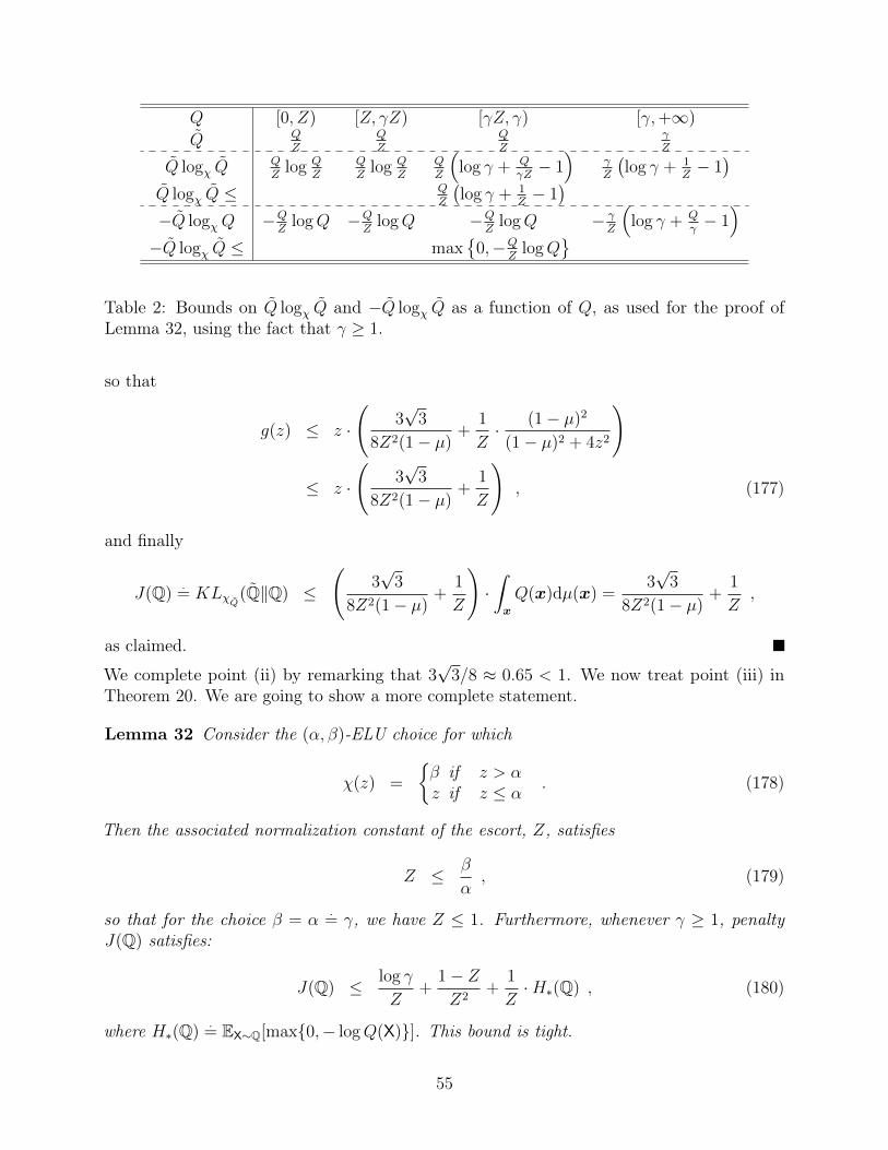
Q [0, Z) [Z, γZ) [γZ, γ) [γ,+∞)

Q QZ

QZ

QZ

γZ

Q logχ QQZ

log QZ

QZ

log QZ

QZ

(log γ + Q

γZ− 1)

γZ

(log γ + 1

Z− 1)

Q logχ Q ≤ QZ

(log γ + 1

Z− 1)

−Q logχQ −QZ

logQ −QZ

logQ −QZ

logQ − γZ

(log γ + Q

γ− 1)

−Q logχ Q ≤ max

0,−QZ

logQ

Table 2: Bounds on Q logχ Q and −Q logχ Q as a function of Q, as used for the proof ofLemma 32, using the fact that γ ≥ 1.

so that

g(z) ≤ z ·(

3√

3

8Z2(1− µ)+

1

Z· (1− µ)2

(1− µ)2 + 4z2

)

≤ z ·(

3√

3

8Z2(1− µ)+

1

Z

), (177)

and finally

J(Q).

= KLχQ(Q‖Q) ≤(

3√

3

8Z2(1− µ)+

1

Z

)·∫x

Q(x)dµ(x) =3√

3

8Z2(1− µ)+

1

Z,

as claimed.

We complete point (ii) by remarking that 3√

3/8 ≈ 0.65 < 1. We now treat point (iii) inTheorem 20. We are going to show a more complete statement.

Lemma 32 Consider the (α, β)-ELU choice for which

χ(z) =

β if z > αz if z ≤ α

. (178)

Then the associated normalization constant of the escort, Z, satisfies

Z ≤ β

α, (179)

so that for the choice β = α.

= γ, we have Z ≤ 1. Furthermore, whenever γ ≥ 1, penaltyJ(Q) satisfies:

J(Q) ≤ log γ

Z+

1− ZZ2

+1

Z·H∗(Q) , (180)

where H∗(Q).

= EX∼Q[max0,− logQ(X)]. This bound is tight.

55

Proof We obtain directly χ(z) ≤ (β/α) · z, from which

Z.

=

∫x

χ(Q(x))dµ(x)

≤ β

α·∫x

Q(x)dµ(x) =β

α. (181)

Then, we remark that if β = α.

= γ ≥ 1, Z ≤ 1 and

logχ(z).

=

∫ z

1

dt

χ(t)=

log γ + z

γ− 1 if z > γ

log z if z ≤ γ, (182)

and we finally obtain,

KLχQ(Q‖Q) =

∫x

Q(x)

∫ Q(x)

Q(x)

1

χ(t)dtdµ(x)

=

∫x

Q(x) logχ Q(x)dµ(x)−∫x

Q(x) logχQ(x)dµ(x)

≤(

log γ

Z+

1− ZZ2

)·∫x

Q(x)dµ(x) +1

Z·H∗(Q)

=log γ

Z+

1− ZZ2

+1

Z·H∗(Q) , (183)

with H∗(Q).

= EX∼Q[max0,− logQ(X)] is a clipping of Shannon’s entropy (which preventsit from being negative). The inequality follows from bounding the two terms in the integraldepending on the value of Q following Table 2.

For tightness, consider the "square" uniform distribution with support an interval [a, a+1]with a ≤ 0, and fix γ = 1, which brings J(Q) = 0 and log γ = 0, Z = 1 and H∗(Q) = 0, soboth bounds in eq. (180) match.

We end up this Section with three additional results related to Theorem 20:

(iv) bounding J(Q) when χ is the signature of q-exponential families, also displaying thatJ(Q) = O(1/Z);

(v) computing exactly J(Q) for a particular χ-family and a member of the χ-family for Q,displaying that J(Q) = θ(1/Z);

(vi) showing how a particular choice for χ that blows up large density regions for some Qcan yield Z arbitrarily large.

We focus now on (v) and pick χ as the signature of popular deformed exponential families,the q-exponential families [3].

Lemma 33 Consider χ(z) = χq(z).

= zq for q > 1. Then for any Q,

Jq(Q) ≤ 1

(q − 1)Z. (184)

56

Proof We get directly

Jq(Q).

= KLχQ(Q‖Q) =

∫x

Q(x)

∫ Q(x)

Q(x)

t−qdtdµ(x)

=1

1− q ·∫x

(Q2−q(x)− Q(x)Q1−q(x))dµ(x)

=1

1− q ·∫x

(1

Z2−q ·Qq(2−q)(x)− 1

Z·Q(x)

)dµ(x)

=1

q − 1·(

1

Z− 1

Z2−q ·∫x

Qq(2−q)(x)dµ(x)

)(185)

≤ 1

(q − 1)Z(186)

since q > 1.

We continue with (v) and pick a particular case for which Q belongs to the χ-family, with anexact computation of J(Q). We choose the 1/2-Gaussian.

Lemma 34 Consider the 1/2-Gaussian on the real interval [−σ, σ], for some σ > 0, whosedensity is given by

Q(x).

=A

σ· [1− (x2/σ2)]2+ , (187)

with A .= 15√

2/32 and [z]+.

= max0, z. Then, for χ being the one of the 1/2-Gaussian, wehave:

J(Q) =3

32

2√σ·(

3π

16− 1√

15√

2

)= θ

(1

Z

). (188)

Proof The 1/2-Gaussian arises from the more general class of q-exponential families, forwhich χ is given in Lemma 33 [6], [41, Chapter 7]. We start at eq. (185):

J(Q).

= KLχQ(Q‖Q) =1

1− q ·(− 1

Z+

1

Z2−q ·∫x

Qq(2−q)(x)dµ(x)

). (189)

Now, consider more specifically the q .= 1/2-Gaussian defined on the real line, for which

Q(x).

= (A/σ)[1− (x2/σ2)]2+. In this case one can obtain that Z = B√σ, B .

= 4√A/3, and

so ∫x

Qq(2−q)(x)dµ(x) =A

34

σ34

·∫ σ

−σ

[1− x2

σ2

] 32

+

dx

= A34σ

14 ·∫ 1

−1

[1− x2

] 32

+dx

=3π

8· A 3

4σ14 , (190)

57

"2 1 "2 p1"2

Z

Figure 12: Consider an initial density Q given by two adjacent squares (in red). Using χ asdefined in eq. (193), the largest values can be blown up β as large as desired so that Z (inblue) is in turn as large as desired (see text; Figure best seen in colour).

since ∫ 1

−1

[1− x2

] 32

+dx =

3π

8(> 1) . (191)

So we obtain, taking into account that A .= 15

√2/32,

J(Q) =3π

4B32 · σ 3

4

· A 34σ

14 − 3

2√A√σ

=1√σ·(

332 · 3π2 · 16

− 332

2√

15√

2

)

=3

32

2√σ·(

3π

16− 1√

15√

2

)≈ 0.9663√

σ

= θ

(1√σ

), (192)

and we can conclude for the proof of Lemma 34.

We finish with (vi) and an example on how picking an escort that blows up large valuesfor a density can indeed make Z very large.

58

Lemma 35 Fix K > 0 and, for some 0 < ε < 1/4, let

χ(z).

=

z if z ≤ ε

ε+ 1logK· (Kz−ε − 1) if z > ε

. (193)

Consider the density Q given in Figure 12. Then, letting Z(Q) denote the normalization ofthe escort of Q, it holds that limK→+∞ Z(Q) = +∞.

Proof It follows that

Z = ε2 +√

1− ε2 ·(ε+

1

logK· (K

√1−ε2−ε − 1)

)= ε2 +

√1− ε2 ·

(ε− 1

logK

)︸ ︷︷ ︸

.=g1(K,ε)

+

√1− ε2

logK·K√

1−ε2−ε︸ ︷︷ ︸.=g2(K,ε)

. (194)

Provided K ≥ exp(4) ≥ exp(1/ε), g1(K, ε) ≥ 0; since ε < 1/4,√

1− ε2 − ε ≥ 1/2 and√1− ε2 ≥ 1/2. Hence, if 0 < ε < 1/4 and K ≥ exp(4), we have

Z ≥√K

2 logK, (195)

and we indeed have limK→+∞ Z = +∞.

21 Many modes for GAN architecturesIn Section 5, we claim that a deep architecture working under the general model specified inSection 5 can accomodate a number of modes of the order of the total dimension of deepsufficient statistics, Ω(d · L). To develop a simple argument, assume that the last layer is theidentity function so we do hot have to care for Hout(x) in Theorem 15. A simple argumentfor this consists in three steps. First, we pick a χ like in Figure 13, whose derivative is goingto zero as many times as necessary. Then,

• (Ω(d · L) critical points at the modes) first computing the critical points using thegradient ∇Qg(z) from Theorem 15, which yields:

∇Qg(z) ∝ ζ(z) +L∑l=1

d∑i=1

ζl,i · χ′l,i(Pχ,bl,i) · ∇z(w>l,iφl−1) , (196)

where the ζ functions are not important, since (i) ζ(z) is always the null vector for Qin

uniform, and (ii) ζl,i depends on z but we can assume it never zeroes (it factors theescort’s density with a non zero constant). Then, using the χ as defined before, we choosethe modes of the inner deformed exponential families (for which ∇z(w>l,iφl−1) = 0) insuch a way that they are located at the critical points of χ, and a different one for eachof them. We obtain a Qg(z) which has up to (an order of) d · L critical points, exactlyat all modes, as claimed;

59

l

Pmode1 Pmode

2 Pmode3

Figure 13: Taking a χ whose derivatives zeroes as many times as needed, and then putting themodes of each inner deformed exponential family where it zeroes makes it easy to accomodateas many modes as needed for a deep architecture.

• (modes at all critical points) since each critical point is located at a mode for one ofthe densities, it is sufficient to ensure that the influence of all other densities in thecurvature of the density is sufficiently small: for this, it is sufficient to then control thesecond derivative of χ in the neighborhood its critical points, making sure it does notexceed a small threshold in absolute value.

Notice that this property is independent from the one which allows to craft escorts that blowhigh density regions (and may yield large Z, Theorem 20, see also Lemma 35 and Figure12), so we can combine both properties and obtain densities for the deep net with both highcontrast around the modes and a large number of modes.

Of course, the χ we choose is very artificial and corresponds to an activation which wouldbe almost piecewise linear, a sort of generalization of the ReLU activation with a large numberof segments or half lines instead of two. Yet, it gives some simple intuition as to how fittingmultimodal densities can indeed happen.

22 Proof of Lemma 21The proof directly comes from Theorem 13: the variational part in the vig-f -GAN identity is:

supT∈R++

X

EX∼P [T (X)]− EX∼Q

[− log(χ•) 1

Q

(−T (X))

]= sup

T∈R++X

EX∼P [−T (X)] + EX∼Q

[log(χ•) 1

Q

(T (X))

], (197)

60

and the DM vs G game in which DM’s objective is to realize:

supΥ:X→R

EX∼P [−Υ(X)] + EX∼Q[udm(Υ(X))] . (198)

Making the correspondence between (198) and the right hand-side of (197) gives the statementof the Lemma.

23 Proof of Lemma 22We recall the utility udm = u (for the sake of readability), and note that it depends on thestate of the world / observation x,

ux(z) = log(χ•) 1Q(x)

(z) . (199)

It follows from Lemma 21 and the definition of χ-logarithms,

u′x(z) =1

χ• 1Q(x)

(z)

=1

Q(x)· χ−1

(Q(x)

z

), (200)

u′′x(z) = − 1

z2· (χ−1)′

(Q(x)

z

)= − 1

z2 · χ′(χ−1

(Q(x)z

)) (≤ 0) . (201)

Putting back all parameters, we obtain the following Arrow-Pratt measure of absolute riskaversion:

aux(z) = −u′′x(z)

u′x(z)

=Q(x)

z2 · χ−1(Q(x)z

)· χ′(χ−1

(Q(x)z

))=

1

z·

Q(x)z

χ−1(Q(x)z

)· χ′(χ−1

(Q(x)z

)) (202)

Since χ : R+ → R+ and is non decreasing, we see that

aux(z) ≥ 0,∀χ, z,x , (203)

and therefore player DM is always risk-averse (this proves point (i)). Define

g(z).

=z · (χ−1)′(z)

χ−1(z), (204)

61

u1

Υ(x)

u(Υ(x))

Υ∗(x)

u2

u1

Υ(x)

u(Υ(x))

Υ∗(x)

Figure 14: Illustration of the optimality conditions for the insurance problem (44), whereinwe pick the risky asset Υ such that for every x ∈ X, marginal utility is equal to the oddsratio. That is, the tangent with slope P (x)/Q(x). (First Diagram) If DM suddenly believesa certain state state x ∈ X is more likely, this pushes the optimal function Υ∗ to the right.(Second Diagram) If we compare two decision makers utilities u1 and u2 such that u2 is morerisk averse than u1. We see that for u2 to consume at the same level as u1, u2 must believex ∈ X is far more likely.

so that

aux(z) =1

z· g(

z

Q(x)

), (205)

and

rux(z) = z · aux(z) = g

(z

Q(x)

). (206)

This proves point (ii). Notably, at the optimum, the dependency on the subjective beliefsdisappears since the optimum (Theorem 11) of Υ∗ = −T ∗ yields:

rux(Υ∗(x)) = g

(χ(Q(x))

Z · χ(P (x))· 1

Q(x)

)= g

(1

χ(P (x))

). (207)

Remark. We can make a connection with a more traditional view of portfolio allocation.The first order conditions for (44) gives us

(∀x ∈ X) u′dm(Υ∗(x)) · Q(x)− P (x) = 0 =⇒ u′dm(Υ∗(x)) =P (x)

Q(x). (208)

From (208) we see that at optimality (equilibrium), Decision Maker picks a portfolio such thathis marginal utility over the risky asset under each state x ∈ X is equal to the correspondingodds ratio. If Decision Maker (for whatever reason) suddenly believes a certain state x0 ∈ X

is more likely (Q(x0) goes up), then with usual assumptions about decreasing marginal utility,it’s intuitive that he will respond by consuming more of Υ(x0). Similarly if compare decisionmakers with differing risk aversion in the risky asset, the more risk averse decision makermust hold much stronger beliefs to consume at the same level as the less risk averse decisionmaker. The optimality condition (208) is illustrated in Figure 14.

62

— Appendix on experiments

24 ArchitecturesWe consider two architectures in our experiments: DCGAN [52] and the multilayer feedforwardnetwork (MLP) used in [47]. Suppose the size of input images is isize-by-isize, the details ofarchitectures are given as follows:

Generator of DCGAN :ConvTranspose(input=100, output=8×isize, stride=1) → BatchNorm→ Activation→

Conv(input=8×isize, output=4×isize, stride=2, padding=1)→ BatchNorm→ Activation→ConvTranspose(input=4×isize, output=2×isize, stride=2, padding=2)→ BatchNorm→ Activation→ConvTranspose(input=2×isize, output= isize, stride=2, padding=1)→ BatchNorm→ Activa-tion → Conv(isize, number of channel, stride=2, padding=1) → Last Activation

Discriminator of DCGAN :Conv(1, 2×isize, stride=2)→ BatchNorm→ LeakyReLU→ Conv(input=2×isize, output=4×isize,

stride=2, padding=1)→ BatchNorm→ LeakyReLU→ Conv(input=4×isize, output=8×isize,stride=2, padding=2)→ BatchNorm→ LeakyReLU→ Conv(input=8×isize, output= 1,stride=2, padding=1)→ Link function

Generator of MLP :z → Linear(100, 1024)→ BatchNorm→ Activation→ Linear(1024, 1024)→ BatchNorm

→ Activation → Linear(1024, isize×isize) → last Activation

Discriminator of MLP :x → Linear(isize×isize, 1024) → ELU → Linear(1024, 1024) → ELU → Linear(1024, 1)

→ Link function

25 Experimental setup for varying the activation func-tion in the generator

Setup. We train adversarial networks with varying activation functions for the generatorson the MNIST [33] and LSUN [61] datasets. In particular, we compare ReLU, Softplus, LeastSquare loss as an example of prop-τ , and µ-ReLU with varying µ in [0, 0.1, ..., 1] by usingthem as the activation functions in all hidden layers of the generators. For all models, we fixthe learning rate to 0.0002 and batch size to 64 throughout all experiments after tuning on ahold-out set.

MNIST. We evaluate the activation functions by using both DCGAN and the MLP usedin [47] as the architectures. As training divergence, we adopt both GAN and Wassersteindistance (WGAN) because GAN belongs to variational f -divergence formulation while WGANdoes not. The link function of the discriminators is specific to the respective divergence, which

63

is sigmoid for GAN and linear for WGAN. We sample random noise z ∈ Uniform100(0, 1)for MLP and z ∈ Gaussian(0, 1) for DCGAN, which is found slightly better than samplingfrom Uniform100(−1, 1). As the best practice, we apply Adam [32] to optimize models withGAN and RMSprop [57] to optimize WGAN based models. For GAN, we train one batch fordiscriminator and one batch for generator iteratively during training. For WGAN, we applyweight clipping with 0.01 and train five batches for discriminator and one batch for generatorinterchangeably during training.

We train all models on the full MNIST training data set and evaluate the performanceon the test set by using the kernel density estimation (KDE). Since the size of imagesaccepted by DCGAN should be n-fold of 16, all images are rescaled to 32-by-32 for all models.Following [47], we apply three-fold cross validation to find optimal bandwidth for the isotropicGaussian kernel of KDE on a hold-out set. To estimate the log probability of the test set, wesample 16k images from the models in the same way as [47]. We observe that the initializationof model parameters has significant influence on performance. Therefore, we conduct threeruns with different random seeds for each experimental setting and report the mean andstandard deviation of the results.

LSUN. We also evaluate all activation functions in consideration for the generator onLSUN natural scene images. We train DCGAN with GAN as the divergence on the towercategory of images, which are rescaled and center-cropped to 64-by-64 pixels, as in [52].Due to the center-cropped images, we apply tanh as last activation of generators instead ofsigmoid for GAN based models.

26 Visual results on MNIST

64

µ µ

0 0.1

0.2 0.3

0.4 0.5

0.6 0.7

0.8 0.9

1

Table 3: MNIST results for GAN_DCGAN at varying µ (µ = 1 is ReLU).

65

µ µ

0 0.1

0.2 0.3

0.4 0.5

0.6 0.7

0.8 0.9

1

Table 4: MNIST results for WGAN_DCGAN at varying µ (µ = 1 is ReLU).

66

µ µ

0 0.1

0.2 0.3

0.4 0.5

0.6 0.7

0.8 0.9

1

Table 5: MNIST results for WGAN_MLP at varying µ (µ = 1 is ReLU).

67

µ µ

0 0.1

0.2 0.3

0.4 0.5

0.6 0.7

0.8 0.9

1

Table 6: MNIST results for GAN_MLP at varying µ (µ = 1 is ReLU).

68

µ µ

0 0.1

0.2 0.3

0.4 0.5

0.6 0.7

0.8 0.9

1

Table 7: LSUN results for GAN_DCGAN at varying µ (µ = 1 is ReLU).

69