gams_toolbox_guide

JULIA LIVERMORE – ENV 859 December 2014

Duke University Nicholas School of the Environment

1

GENERAL ADDITIVE MODEL TOOLBOX

USAGE GUIDE

CONTENTS

Toolbox Purpose: ....................................................................................................................................................................................... 2

Background: .............................................................................................................................................................................................. 2

NOAA NEFSC Trawl Survey Data: ....................................................................................................................................................... 2

General Additive Models: ................................................................................................................................................................... 3

Trawl Data Usage in GAMs: ................................................................................................................................................................ 3

Environmental Parameter Data: ........................................................................................................................................................ 4

Species of Interest: ............................................................................................................................................................................... 6

Step-By-Step Instructions/Best Practices:............................................................................................................................................... 6

Preparation: .......................................................................................................................................................................................... 6

Step 1: Data Extraction from the NOAA Trawl Survey Data File ................................................................................................... 6

Step 2: Fitting the General Additive Model ...................................................................................................................................... 7

Step 3: Predicting your GAM ............................................................................................................................................................ 11

Step 4: Applying the Results to Create a Habitat Raster ............................................................................................................. 13

Appendix: ................................................................................................................................................................................................. 17

FOR MODELING THE

HABITAT OF SPECIES WITH

SHIFTING DISTRIBUTIONS

ON THE NORTHEAST

LARGE MARINE

ECOSYSTEM

BLACK SEA BASS



2

TOOLBOX PURPOSE:

This toolbox allows a user to run general additive models for three species of fish in on the Mid-

Atlantic Bight and in the Gulf of Maine using five simple steps. Selected species include black

sea bass, scup, and red hake. Models can be run using NOAA trawl data from the fall of 2013

and the spring of 2014. The user has the ability to select what variables to include within the

models by running the Step 2B tool multiple times and changing what environmental data

should be included (model evaluation is incorporated into the toolbox). The outputs of this

toolbox include: a text summary of model performance, a text summary of model evaluation, a

PNG of the receiver operator curve and Youden Index cutoff value, a raster of probability of

encountering selected species, and a raster of Youden Index cutoff determined habitat regions.

All tools have directions within the help tab. Follow the directions very carefully to ensure that

your outputs are what you intend them to be.

NOTE: All models are run using R software through the Duke Marine Geospatial Ecology Lab's

Marine Geospatial Ecology Toolbox (http://mgel.env.duke.edu/mget/). You will need this

toolbox, R software, and the ArcGIS Spatial Analyst Extension to run these tools on your

computer.

BACKGROUND:

NOAA NEFSC TRAWL SURVEY DATA:

The National Oceanic and Atmospheric Administration (NOAA) Northeast Fisheries Science

Center (NEFSC) conducts two multispecies bottom trawl surveys per year. One survey is carried

out in the fall (September – October) and the other during the spring (February – April). These

surveys aim to monitor trends in abundance, biomass, and recruitment; monitor the geographic

distribution of species; monitor ecosystem changes; monitor trends in biological parameters

(growth, mortality, and maturation rates) of the stocks; and collect other environmental data.

The autumn survey has been conducted annually since 1963 (51 years); the spring survey began

in 1968 (46 years).

The surveys are conducted using a stratified random design. Station locations are randomly

selected within geographic strata. The same boat, the FSV Henry B. Bigelow, is used every year

and a 4-seam, 3-bridle box net is used to collect marine organisms. This methodology was

created through collaboration between industry representatives, academia/gear researchers,

and NEFSC scientists.

Key attributes of the scientific trawling system include:

1) Representative sample of a variety of species and sizes

2) Ability to sample a variety of habitats

3) Maximum catchability between the wing ends and minimum sampling between the

wing ends and doors

http://mgel.env.duke.edu/mget/



3

4) Consistent wind speed

5) Consistent headrope height

6) Consistent bottom contact

7) Easily Maintained

All benthic survey information acquired from the NOAA Fisheries Service Ecosystem Surveys

Branch: http://nefsc.noaa.gov/esb/mainpage/. For more information specifically on the survey,

see http://www.nefsc.noaa.gov/groundfish/meetings/johnston.pdf.

GENERAL ADDITIVE MODELS:

The generalized additive model (GAM) is possibly the most well-developed method for modeling

fish habitats (Valavanis et al., 2008) because it offers an objective way to predict abundance or

biomass according to the known ecology of the fish species over broad geographic areas (Drexler

and Ainsworth, 2013).

The GAM emerged from the more simple generalized linear model (GLM) but it allows several

transformations to be applied to the individual independent variables before adding them to the

model (Knudby et al., 2010). GAMs are now widely applied in fisheries science because they are

straightforward extensions of GLMs, which allow linear and other parametric terms to be replaced

by smoothing functions. Hence, GAMs allow increased flexibility in the model fitting as compared

to GLMs (Drexler and Ainsworth, 2013). This method has been used to map relationships between

a variety of species and their environments. For example, Drexler and Ainsworth (2013) applied a

GAM approach to climate scale oceanographic conditions data and a large fisheries

independent data set (SEAMAP) in order to describe areas of high abundances of pink shrimp

(Farfantepenaeus duroarum) in the Gulf of Mexico.

Nevertheless, the GAM method has one major limitation with respect to fisheries science; GAMs

are additive and therefore cannot deal with interaction effects. Be that as it may, they are still

extremely useful and can be run in R using the ‘mgcv’ or ‘gam’. The Akaike Information Criterion

(AIC) can be used to determine variable inclusion (Knudby et al., 2010) and the link function can

be used between the expected values of the response variable and explanatory variables that

ensures that the fitted values make sense (Valavanis et al., 2008).

TRAWL DATA USAGE IN GAMS:

GAMs are widely accepted as one of the most accurate and objective ways to model fish habitat.

The data collected through the NEFSC benthic trawl surveys is highly suitable for GAMs because

of its random stratified sampling method. Proper data extraction can produce presence and

absence point locations for any species surveyed. Presence and absence point locations can

then be sampled with respect to a variety of environmental parameters to create an input table

for use in a general additive model.

Due to how the data is collected during the trawl survey, a few model functions must be set to

match the binomial (presence-absence) format of the data. The following functions have already

been set within the toolbox tools:

http://nefsc.noaa.gov/esb/mainpage/

http://www.nefsc.noaa.gov/groundfish/meetings/johnston.pdf



4

Model Type: General Additive Model

Model Family: binomial

R Toolbox: mgcv

Link function: logit

Smoothing parameter estimation method: GCV.Cp

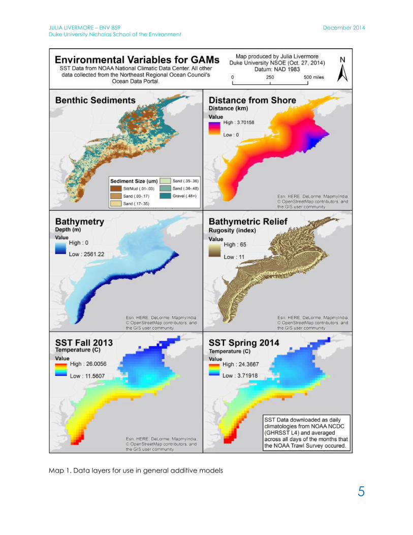
ENVIRONMENTAL PARAMETER DATA:

Up to five environmental variables may be included within each model. Potential variables are:

Benthic sediments – raster data downloaded from the Northeast Regional Ocean Council

(NROC) Ocean Data Portal

Bathymetry – raster data downloaded from the NROC Ocean Data Portal

Bathymetric Relief – raster data downloaded from the NROC Ocean Data Portal

Distance from Shore – raster layer created by Julia Livermore using the ESRI Spatial Analyst

Extension’s Euclidian Distance Tool from a shoreline shapefile obtained through the NROC

Ocean Data Portal

Sea Surface Temperature – only the SST layer matching the season of the sampling should

be included

o Sea Surface Temperature for Fall 2013 – raster layer created by Julia Livermore by

using the Marine Geospatial Ecology Toolbox (MGET) to download daily

climatologies (from the National Climatic Data Center – NCDC) for all days that

the trawl survey occurred. All daily climatologies were then averaged to produce

a single raster layer of sea surface temperatures for the entire temporal range

during which the survey occurred in the fall.

o Sea Surface Temperature for Spring 2014 - raster layer created by Julia Livermore

by using MGET to download daily climatologies (from the NCDC) for all days that

the trawl survey occurred. All daily climatologies were then averaged to produce

a single raster layer of sea surface temperatures for the entire temporal range

during which the survey occurred in the spring.

In Step 1 of the toolbox, presence and absence point locations will be sampled to record the

value of all environmental variables at each location. These data will be saved as a dBase table

for use in later tools to actually run the models.

See the map on the next page for a visual representation of the six data layers



5

Map 1. Data layers for use in general additive models



6

SPECIES OF INTEREST:

Three species were selected for analysis. These species include black sea bass, scup, and red hake.

All three fish species are thought to be on the move geographically due to changing

environmental conditions. Each species has a unique life history and may show very different

species assemblage shifts.

STEP-BY-STEP INSTRUCTIONS/BEST PRACTICES:

PREPARATION:

Download the entire zipped GAMs folder and unzip it in a location of your choosing.

o Make sure you have sufficient space on your computer or server before running

these tools. Some of the tools create many files to produce final outputs. These

intermediary files will be deleted, but do take up some space during processing.

Open the GAM.mxd in ArcGIS to look at the environmental data.

Set the GAMs folder as the ‘Home’ location using the Catalog within ArcGIS or

ArcCatalog.

o Feel free to look around within the data, docs, scratch, and scripts folders, but:

DO NOT move any files.

DO NOT change any file names.

DO NOT edit any of the scripts in the scripts folder.

o If you make any changes, the tools in the GAMs.tbx will not function.

Open up the GAMs toolbox to get started.

o NOTE: Always be sure to refresh the entire GAMs folder after running each tool.

This will ensure that you see your new files and that they load properly when

added to the map. This will also guarantee that any temporary files from

processing are deleted, which will save memory on your drive and make later

steps simpler.

STEP 1: DATA EXTRACTION FROM THE NOAA TRAWL SURVEY DATA FILE

This tool will extract data from a csv of trawl data based on user inputs. The user can select

which species and season to extract data for. The output of this tool is a dBase file that can be

used as the input to steps 2A and 2B.

Note: The Trawl_Data.csv containing the data is not the original file provided by the NEFSC. The

original file dates back to 1963 and includes over 100 species; thus, it is EXTREMEMLY large. The

Trawl_Data.csv is original data, but any species not of interest have been removed, and surveys

prior to Fall 2013 have also been removed. A presence-absence column has also been added

to specify which points a species was found versus not found. Please contact Julia Livermore at

[email protected] if you have any questions about how this was done in R.

Open the Step 1 (Data Extraction) script by double clicking on it.

Select the Data folder within the GAMs folder as your workspace.

o The original data from which data extraction will occur is contained within the

data folder. You must select this as your workspace or the tool will not work.

mailto:[email protected]



7

Set your scratch workspace as the Scratch folder in the GAMs folder.

Select the species you want to model habitat for from the dropdown menu.

o BSB = Black Sea Bass

o SCUP = Scup

o RED HAKE = Red Hake

Select the season you want to model the species’ habitat for from the dropdown menu.

o FALL = Fall 2013

o SPRING = Spring 2014

Your inputs should look similar to this:

Run the tool by clicking ‘OK’

Check your Scratch folder for a new dBase table titled SPECIES_SEASONno0s.dbf where

SPECIES and SEASON are equal to what you selected in the tool.

STEP 2: FITTING THE GENERAL ADDITIVE MODEL

This step has two parts. The first part will use tool Step 2A (Fit GAM) to run a GAM using all five

environmental parameters. The user will be able to look at the output from R to determine what

parameters he or she wants to include in the final model. Selecting which terms to include in the

final model can be a difficult and confusing process. The user should be comfortable with model

selection prior to using this tool. For more information on this process, refer to:

https://stat.ethz.ch/R-manual/R-devel/library/mgcv/html/gam.selection.html

Double click on Step 2A (Fit GAM) to open the tool.

Select the dBase table you created in Step 1 (which should be in the Scratch folder) as

the Input Table.

For the Output Name, type in SPECIES_SEASON where SPECIES and SEASON are equal to

what you selected in Step 1.

o DO NOT add an extension to this, as extensions have already been incorporated

into the model and will be added during processing.

Select the Scratch folder again as your Scratch Workspace.

Your inputs should look similar to this:

https://stat.ethz.ch/R-manual/R-devel/library/mgcv/html/gam.selection.html



8

Run the tool by clicking ‘OK.’

Check your Scratch Folder for a new .Rdata and text file

o The text file will be titled SPECIES_SEASON_summary.txt.

o The .Rdata file will be called SPECIES_SEASON.Rdata.

Open the text summary file and look at your model results.

o For black sea bass in the spring, the results are as follows:



9

Look over the summary to determine which terms should actually be included in your

final model.

o In this example, only bathymetry and sea surface temperature appear to be

important to the distribution of the species. Thus, we will only include these two

variables in the final model.

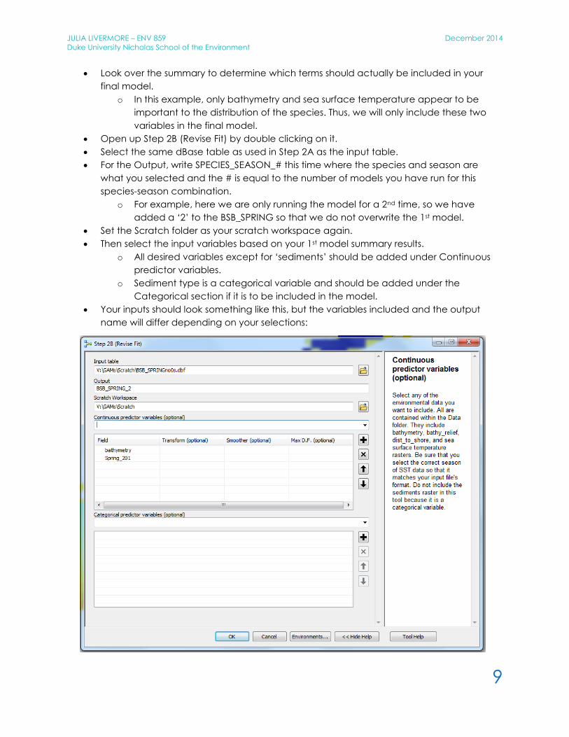
Open up Step 2B (Revise Fit) by double clicking on it.

Select the same dBase table as used in Step 2A as the input table.

For the Output, write SPECIES_SEASON_# this time where the species and season are

what you selected and the # is equal to the number of models you have run for this

species-season combination.

o For example, here we are only running the model for a 2nd time, so we have

added a ‘2’ to the BSB_SPRING so that we do not overwrite the 1st model.

Set the Scratch folder as your scratch workspace again.

Then select the input variables based on your 1st model summary results.

o All desired variables except for ‘sediments’ should be added under Continuous

predictor variables.

o Sediment type is a categorical variable and should be added under the

Categorical section if it is to be included in the model.

Your inputs should look something like this, but the variables included and the output

name will differ depending on your selections:



10

o Since only bathymetry and SST were significant, they are the only variables

included here.

o Note: Selecting variables based solely on significance is not good practice.

Please research model selection methods before making your final decisions. We

are using these two variables in this step simply for demonstration.

Open the text summary results from your new model (this file and a new .Rdata file

should be in your scratch folder).

o You can see that the percent deviance explained decreased and the UBRE

score grew, so this model is actually worse than the first one.

Use the Step 2B tool to try different term combinations until you have a model that you

are satisfied with.

o Just make sure to change the number at the end of SPECIES_SEASON_# each

time so that you do not overwrite any of your files. This will allow you to compare

your results side by side.



11

STEP 3: PREDICTING YOUR GAM

Step 3 will test your model out by applying some of the original data to the model output. A text

summary of model predictions and Receiver Operator Curve (ROC) results will be produced,

along with a colorized PNG image file of the ROC and Youden-Index cutoff.

Open Step 3 (Predict GAM) by double clicking on it.

For the Model Rdata file, select the .Rdata file of your best model (this should be in your

scratch folder).

o In this example, we are using the 1st model just for simplicity. This is probably NOT

the best model.

Next, type SPECIES_SEASON for the Output File Name, where SPECIES and SEASON match

your earlier selections.

Select the Scratch folder again for the Scratch Workspace.

Your inputs should look something like this.

Open up the new text file in your scratch folder. This file should be named

SPECIES_SEASON_SumStats.txt.

o In this example, the model produced the following results.



12

There should also be a PNG of the ROC curve showing where the Youden Index Cutoff is

located.

o In this example, the results look like this.



13

If you are satisfied with your model’s performance, proceed to step 4. If you are not

satisfied, return to Step 2B and repeat Steps 2B and 3 until you have a model that you are

pleased with.

STEP 4: APPLYING THE RESULTS TO CREATE A HABITAT RASTER

This tool allows the user to input the estimate values of the term parametric coefficients to

produce a probability raster and a habitat raster for the selected species and season. The

probability raster will indicate the probability of encountering the selected species at each

location. The habitat raster will indicate likely areas of habitat, based on the Youden Index/ ROC

cutoff.

Double click on Step 4 (Apply Results) to open up the tool/script.

Select the Data folder as the Workspace.

o This is very important because all of the environmental data rasters are in the

data folder and are needed to make this tool work.

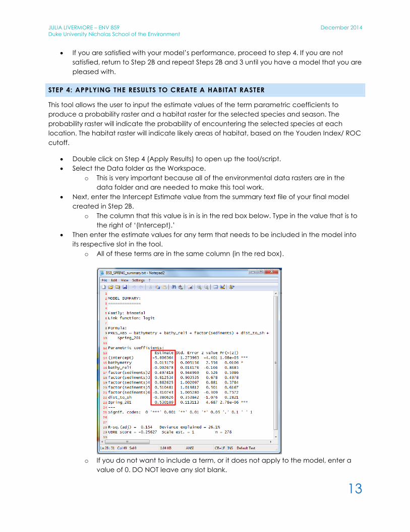
Next, enter the Intercept Estimate value from the summary text file of your final model

created in Step 2B.

o The column that this value is in is in the red box below. Type in the value that is to

the right of ‘(Intercept).’

Then enter the estimate values for any term that needs to be included in the model into

its respective slot in the tool.

o All of these terms are in the same column (in the red box).

o If you do not want to include a term, or it does not apply to the model, enter a

value of 0. DO NOT leave any slot blank.



14

Write SPECIES_SEASON again for the Output file name.

Finally, enter the Youden Index cutoff value into the last slot.

o This value is listed in the SPECIES_SEASON_SumStats.txt file or in on the

SPECIES_SEASON.png (circled in red in the diagram below).

Your results should look something like this, but the values will depend on your model.

Refresh your data folder and check for two new rasters titled SPECIES_SEASON_Prob.img

and SPECIES_SEASON_habitat.img.

o The probability raster will show the probability of encountering a species at every

point.



15

o The habitat raster will separate the probability raster into habitat and non-habitat

based on the ROC cutoff value, which is the most objective way to determine

what percentages are likely to indicate habitat.

Your final results will depend on your model.

o Here are the results from the 1st Black Sea Bass Spring 2014 model used as an

example throughout this guide (the model including all environmental terms from

Step 2A, Step 3, and Step 4).

Map 2. This map demonstrates what a probability raster for the black sea bass (spring 2014)

GAM will look like, if all model terms/environmental parameters are included.



16

Map 3. This map demonstrates what the same model’s habitat raster will look like, based on the

ROC determined cutoff of 0.166.

REFERENCES:

Johnston, Robert (2012) NEFSC Multispecies Bottom Trawl Survey. NOAA Fisheries Service

Ecosystem Surveys Branch.

http://www.nefsc.noaa.gov/groundfish/meetings/johnston.pdf

Knudby A, Brenning A, LeDrew E (2010) New approaches to modelling fish–habitat relationships.

Ecological Modeling 221(3): 503-511.

Drexler M, Ainsworth CH (2013) Generalize additive models used to predict species abundance

in the Gulf of Mexico: An ecosystem modeling tool. PLoS One 8(5): e64458.

Valavanis VD, Pierce P, Zuur A, Palialexis A, Saveliev A, Katara I, Wang J (2008) Modeling of

essential fish habitat based on remote sensing, spatial analysis and GIS. Developments in

Hydrobiology 203: 5-20.

http://link.springer.com/search?facet-author=%22Vasilis+D.+Valavanis%22

http://link.springer.com/search?facet-author=%22Vasilis+D.+Valavanis%22

http://link.springer.com/search?facet-author=%22Alain+F.+Zuur%22

http://link.springer.com/search?facet-author=%22Andreas+Palialexis%22

http://link.springer.com/search?facet-author=%22Anatoly+Saveliev%22

http://link.springer.com/search?facet-author=%22Isidora+Katara%22

http://link.springer.com/search?facet-author=%22Jianjun+Wang%22



17

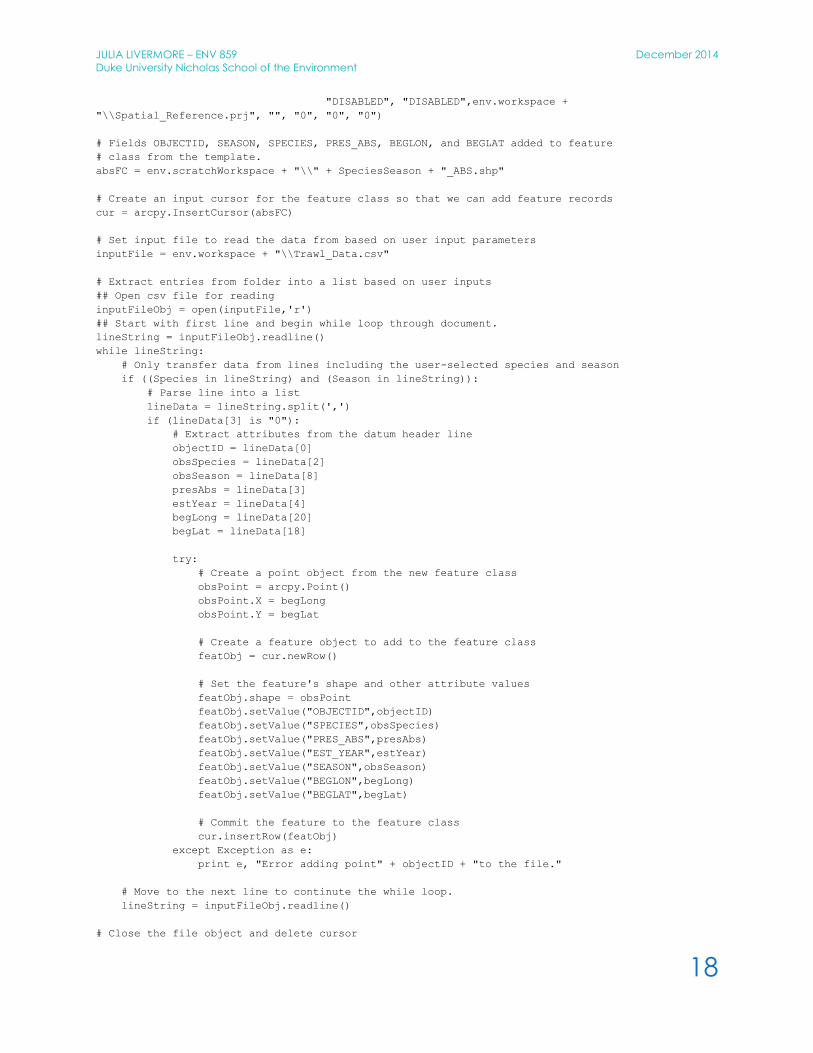
APPENDIX:

Script 1: Step 1 (Data Extraction)

##-------------------------------------------------------------------------------------

## Script Name: Data_Extraction.py

##

## Description: New England GAM tool for Scup, Black Sea Bass, and Red Hake.

## This tool will extract presence and absence points for a user

## selected species and season and create a shapefile of those points.

## Then it will sample input rasters (environmental data) for the points

## in the shapefile and produce a DBase table of the values. Next

## it will remove any points for which any environmental data is missing.

## This table will serve as the input for the Fit GAM tool in the Marine

## Geospatial Ecology Toolbox.

##

## Note: The user must have the MGET toolbox installed on his or her

## computer for this tool to function. See http://mgel.env.duke.edu/mget

## for more information.

##

## This tool also requires the spatial analyst extension in ArcGIS.

##

## Created: November 2014

## Author: Julia Livermore - [email protected] (for Master's Research)

##-------------------------------------------------------------------------------------

# Import system modules

import arcpy, os, sys

from arcpy import env

from arcpy.sa import *

# Set environmental settings

env.workspace = sys.argv[1]

env.scratchWorkspace = sys.argv[2]

env.overwriteOutput = True

# Check out the ArcGIS Spatial Analyst extension license

arcpy.CheckOutExtension("Spatial")

#--------------------------------------------------------------------------------

# Data Extraction from NOAA Trawl Survey Data

arcpy.AddMessage("Extracting data.")

#Get user input on species and season (only options are Spring 2014 and Fall 2103)

## These options will be explicitly described in the ArcGIS tool script.

Species = arcpy.GetParameterAsText(2)

### BSB, RED HAKE, and SCUP

Season = arcpy.GetParameterAsText(3)

### SPRING, FALL

### Explain that spring is spring 2014 and fall is fall 2013

# Create string for simpler paths

SpeciesSeason = str(Species + "_" + Season)

# Create a shapefile of absence points from the survey data

# Process: Create Feature Class

arcpy.CreateFeatureclass_management(env.scratchWorkspace, SpeciesSeason + "_ABS.shp", "POINT",

env.workspace + "\\Pres_Abs_Template.shp",



18

"DISABLED", "DISABLED",env.workspace +

"\\Spatial_Reference.prj", "", "0", "0", "0")

# Fields OBJECTID, SEASON, SPECIES, PRES_ABS, BEGLON, and BEGLAT added to feature

# class from the template.

absFC = env.scratchWorkspace + "\\" + SpeciesSeason + "_ABS.shp"

# Create an input cursor for the feature class so that we can add feature records

cur = arcpy.InsertCursor(absFC)

# Set input file to read the data from based on user input parameters

inputFile = env.workspace + "\\Trawl_Data.csv"

# Extract entries from folder into a list based on user inputs

## Open csv file for reading

inputFileObj = open(inputFile,'r')

## Start with first line and begin while loop through document.

lineString = inputFileObj.readline()

while lineString:

# Only transfer data from lines including the user-selected species and season

if ((Species in lineString) and (Season in lineString)):

# Parse line into a list

lineData = lineString.split(',')

if (lineData[3] is "0"):

# Extract attributes from the datum header line

objectID = lineData[0]

obsSpecies = lineData[2]

obsSeason = lineData[8]

presAbs = lineData[3]

estYear = lineData[4]

begLong = lineData[20]

begLat = lineData[18]

try:

# Create a point object from the new feature class

obsPoint = arcpy.Point()

obsPoint.X = begLong

obsPoint.Y = begLat

# Create a feature object to add to the feature class

featObj = cur.newRow()

# Set the feature's shape and other attribute values

featObj.shape = obsPoint

featObj.setValue("OBJECTID",objectID)

featObj.setValue("SPECIES",obsSpecies)

featObj.setValue("PRES_ABS",presAbs)

featObj.setValue("EST_YEAR",estYear)

featObj.setValue("SEASON",obsSeason)

featObj.setValue("BEGLON",begLong)

featObj.setValue("BEGLAT",begLat)

# Commit the feature to the feature class

cur.insertRow(featObj)

except Exception as e:

print e, "Error adding point" + objectID + "to the file."

# Move to the next line to continute the while loop.


# Close the file object and delete cursor



19

inputFileObj.close()

del cur

# Create a shapefile of absence points from the survey data

# Set Local variables:

Pres_Abs_Template_shp = env.workspace + "\\Pres_Abs_Template.shp"

outputShapefile = SpeciesSeason + "_PRES.shp"

# Process: Create Feature Class

arcpy.CreateFeatureclass_management(env.scratchWorkspace, outputShapefile, "POINT",

Pres_Abs_Template_shp, "DISABLED", "DISABLED",

env.workspace + "\\Spatial_Reference.prj","", "0", "0", "0")

# Fields OBJECTID, SEASON, SPECIES, PRES_ABS, BEGLON, and BEGLAT added to feature

# class from the template.

presFC = env.scratchWorkspace + "\\" + SpeciesSeason + "_PRES.shp"

# Create an input cursor for the feature class so that we can add feature records

cur = arcpy.InsertCursor(presFC)

# Set input file to read the data from based on user input parameters

inputFile = env.workspace + "\\Trawl_Data.csv"

# Extract entries from folder into a list based on user inputs

## Open csv file for reading

inputFileObj = open(inputFile,'r')

## Start with first line and begin while loop through document.


while lineString:

# Only transfer data from lines including the user-selected species and season

if ((Species in lineString) and (Season in lineString)):

# Parse line into a list

lineData = lineString.split(',')

if (lineData[3] is "1"):

# Extract attributes from the datum header line

objectID = lineData[0]

obsSpecies = lineData[2]

obsSeason = lineData[8]

presAbs = lineData[3]

estYear = lineData[4]

begLong = lineData[20]

begLat = lineData[18]

try:

# Create a point object from the new feature class

obsPoint = arcpy.Point()

obsPoint.X = begLong

obsPoint.Y = begLat

# Create a feature object to add to the feature class

featObj = cur.newRow()

# Set the feature's shape and other attribute values

featObj.shape = obsPoint

featObj.setValue("OBJECTID",objectID)

featObj.setValue("SPECIES",obsSpecies)

featObj.setValue("PRES_ABS",presAbs)

featObj.setValue("EST_YEAR",estYear)

featObj.setValue("SEASON",obsSeason)

featObj.setValue("BEGLON",begLong)

featObj.setValue("BEGLAT",begLat)



20

# Commit the feature to the feature class

cur.insertRow(featObj)

except Exception as e:

print e, "Error adding point" + objectID + "to the file."

# Move to the next line to continute the while loop.


# Close the file object and delete cursor

inputFileObj.close()

del cur

arcpy.AddMessage("2 new feature classes have been created in the scratch folder.")

#--------------------------------------------------------------------------------

# Sampling environmental data with datapoints from trawl survey

# Set local variables

sampleMethod = "NEAREST"

if Season is "FALL":

inRasters = ["bathymetry.img",

"bathy_relief.img",

"sediments.img",

"dist_to_shore.img",

"Fall_2013_SST.img"]

else:

inRasters = ["bathymetry.img",

"bathy_relief.img",

"sediments.img",

"dist_to_shore.img",

"Spring_2014_SST.img"]

# Execute Sample

Sample(inRasters, absFC, env.scratchWorkspace + "\\" + SpeciesSeason + "_SampAb.dbf",

sampleMethod)

Sample(inRasters, presFC, env.scratchWorkspace + "\\" + SpeciesSeason + "_SampPr.dbf",

sampleMethod)

arcpy.AddMessage("2 new dBase tables have been created in the scratch folder.")

# Add field for presence-absence values to the tables

arcpy.AddField_management(env.scratchWorkspace + "\\" + SpeciesSeason +

"_SampAb.dbf","PRES_ABS","SHORT")

arcpy.AddField_management(env.scratchWorkspace + "\\" + SpeciesSeason +

"_SampPr.dbf","PRES_ABS","SHORT")

# Fill in values

arcpy.CalculateField_management(env.scratchWorkspace + "\\" + SpeciesSeason +

"_SampAb.dbf","PRES_ABS",0)

arcpy.CalculateField_management(env.scratchWorkspace + "\\" + SpeciesSeason +

"_SampPr.dbf","PRES_ABS",1)

# Merge the two tables into one

arcpy.Merge_management([env.scratchWorkspace + "\\" + SpeciesSeason + "_SampAb.dbf",

env.scratchWorkspace + "\\" + SpeciesSeason + "_SampPr.dbf"],

env.scratchWorkspace + "\\" + SpeciesSeason + ".dbf")

arcpy.AddMessage("1 new dBase table has been created in the scratch folder.")



21

#------------------------------------------------------------------------------------------------

# Select only values where sample data exists for all sampled rasters

# Set input variables

in_feature = env.scratchWorkspace + "\\" + SpeciesSeason + ".dbf"

out_table = env.scratchWorkspace + "\\" + SpeciesSeason + "no0s.dbf"

if Season is "FALL":

where_clause = """"bathymetry" < 0 AND "bathy_reli" > 0 AND "sediments" > 0 AND "dist_to_sh"

> 0 AND "Fall_2013_" > 0"""

else:

where_clause = """"bathymetry" < 0 AND "bathy_reli" > 0 AND "sediments" > 0 AND "dist_to_sh"

> 0 AND "Spring_201" > 0"""

# Execute table select

arcpy.TableSelect_analysis(in_feature, out_table, where_clause)

# Delete all temporary files

arcpy.AddWarning("Deleting temporary files.")

os.remove(env.scratchWorkspace + "\\" + SpeciesSeason + ".dbf")

os.remove(env.scratchWorkspace + "\\" + SpeciesSeason + "_PRES.shp")

os.remove(env.scratchWorkspace + "\\" + SpeciesSeason + "_ABS.shp")

os.remove(env.scratchWorkspace + "\\" + SpeciesSeason + "_PRES.dbf")

os.remove(env.scratchWorkspace + "\\" + SpeciesSeason + "_ABS.dbf")

os.remove(env.scratchWorkspace + "\\" + SpeciesSeason + "_SampPr.dbf")

os.remove(env.scratchWorkspace + "\\" + SpeciesSeason + "_SampAb.dbf")

os.remove(env.scratchWorkspace + "\\" + SpeciesSeason + "_ABS.prj")

os.remove(env.scratchWorkspace + "\\" + SpeciesSeason + "_PRES.prj")

arcpy.AddMessage("One .dbf file has been added to the scratch folder.")

arcpy.AddMessage("The final .dbf table should be used as the input for the Fit GAM tool in

MGET.")

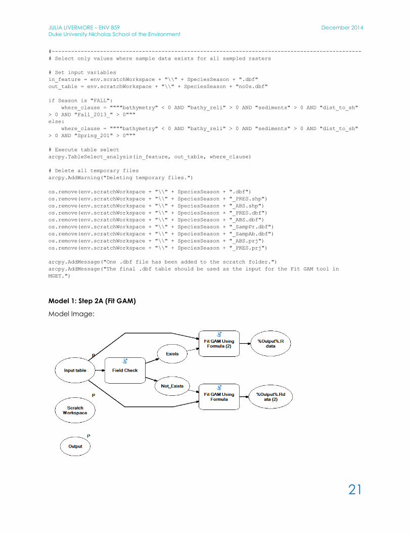
Model 1: Step 2A (Fit GAM)

Model Image:



22

Model Python Script:

# -*- coding: utf-8 -*-

# ---------------------------------------------------------------------------

# 2a.py

# Created on: 2014-12-02 16:26:23.00000

# (generated by ArcGIS/ModelBuilder)

# Usage: 2a <Input_table> <Output> <Scratch_Workspace>

# Description:

# ---------------------------------------------------------------------------

# Import arcpy module

import arcpy

# Load required toolboxes

arcpy.ImportToolbox("V:/GAMs/GAMs.tbx")

arcpy.ImportToolbox("C:/Program Files/GeoEco/ArcGISToolbox/Marine Geospatial Ecology Tools.tbx")

# Script arguments

Input_table = arcpy.GetParameterAsText(0)

Output = arcpy.GetParameterAsText(1)

Scratch_Workspace = arcpy.GetParameterAsText(2)

# Local variables:

v_Output__Rdata__2_ = Input_table

Exists = Input_table

v_Output__Rdata = Exists

Not_Exists = Input_table

# Process: Field Check

arcpy.gp.toolbox = "V:/GAMs/GAMs.tbx";

# Warning: the toolbox V:/GAMs/GAMs.tbx DOES NOT have an alias.

# Please assign this toolbox an alias to avoid tool name collisions

# And replace arcpy.gp.FieldCheck(...) with arcpy.FieldCheck_ALIAS(...)

arcpy.gp.FieldCheck(Input_table, "Spring_201")

# Process: Fit GAM Using Formula

arcpy.GAMFitToArcGISTableUsingFormula_GeoEco(Input_table, v_Output__Rdata__2_, "PRES_ABS ~

bathymetry + bathy_reli + factor(sediments) + dist_to_sh + Fall_2013_", "binomial", "mgcv", "",

"logit", "", "", "GCV.Cp", "outer", "newton", "false", "1", "", "", "", "", "false", "true",

"false", "false", "false", "false", "false", "png", "1000", "3000", "3000", "10", "white")

# Process: Fit GAM Using Formula (2)

arcpy.GAMFitToArcGISTableUsingFormula_GeoEco(Input_table, v_Output__Rdata, "PRES_ABS ~ bathymetry

+ bathy_reli + factor(sediments) + dist_to_sh + Spring_201", "binomial", "mgcv", "", "logit", "",

"", "GCV.Cp", "outer", "newton", "false", "1", "", "", "", "", "false", "true", "false", "false",

"false", "false", "false", "png", "1000", "3000", "3000", "10", "white")



23

Model 2: Step 2B (Revise Fit)

Model Image:


# -*- coding: utf-8 -*-

# ---------------------------------------------------------------------------

# 2b.py

# Created on: 2014-12-02 16:26:36.00000


# Usage: 2b <Input_table> <Output> <Scratch_Workspace> <Continuous_predictor_variables>

<Categorical_predictor_variables>

# Description:

# ---------------------------------------------------------------------------


import arcpy



# Script arguments

Input_table = arcpy.GetParameterAsText(0)

Output = arcpy.GetParameterAsText(1)


Continuous_predictor_variables = arcpy.GetParameterAsText(3)

Categorical_predictor_variables = arcpy.GetParameterAsText(4)

# Local variables:

v_Output__Rdata = Input_table

# Process: Fit GAM

arcpy.GAMFitToArcGISTable_GeoEco(Input_table, v_Output__Rdata, "PRES_ABS", "binomial", "mgcv",

Continuous_predictor_variables, Categorical_predictor_variables, "", "", "", "", "logit", "", "",

"GCV.Cp", "outer", "newton", "false", "1", "", "true", "true", "false", "false", "false",

"false", "false", "png", "1000", "3000", "3000", "10", "white")



24

Model 3: Step 3 (Predict GAM)

Model Image:


# -*- coding: utf-8 -*-

# ---------------------------------------------------------------------------

# 3.py

# Created on: 2014-12-02 16:26:46.00000


# Usage: 3 <Model_Rdata_File> <Output_File_Name> <Scratch_Workspace>

# Description:

# ---------------------------------------------------------------------------


import arcpy



# Script arguments

Model_Rdata_File = arcpy.GetParameterAsText(0)

Output_File_Name = arcpy.GetParameterAsText(1)


# Local variables:

v_Output_File_Name__png = Model_Rdata_File

v_Output_File_Name__SumStats_txt = Model_Rdata_File

Updated_table = Model_Rdata_File

Output_cutoff = Model_Rdata_File

# Process: Predict GAM From Table

arcpy.GAMPredictFromArcGISTable_GeoEco(Model_Rdata_File, "", "", "", "", "true", "", "",

v_Output_File_Name__png, "tpr", "fpr", "true", v_Output_File_Name__SumStats_txt, "1000", "3000",

"3000", "10", "white")



25

Script 2: Step 4 (Apply Results)

##-------------------------------------------------------------------------------------

## Script Name: GAM_Raster_Creation.py

##

## Description: This tool will create a probability raster of the likelihood of

## encountering the species at each location. A raster of habitat

## will also be created based on the ROC-determined probability

## cutoff.

##

## This tool also requires the spatial analyst extension in ArcGIS.

##

## Created: November 2014

## Author: Julia Livermore - [email protected] (for Master's Research)

##-------------------------------------------------------------------------------------


import arcpy, os, sys

from arcpy import env

from arcpy.sa import *

# Set environmental settings

env.workspace = sys.argv[1] ## Set to Data folder again

env.overwriteOutput = True

env.mask = env.workspace + "\\final_mask.img"

# Check out the ArcGIS Spatial Analyst extension license

arcpy.CheckOutExtension("Spatial")

#-------------------------------------------------------------------------------------

# Have user input the estimate values from the summary text file from Step 2.

## May include bathymetry, bathymetric relief, SST, distance from shore

## and/or any of the six sediment rasters.

intercept = arcpy.GetParameterAsText(1)

bathymetry_factor = arcpy.GetParameterAsText(2)

bathy_reli_factor = arcpy.GetParameterAsText(3)

sediments1_factor = arcpy.GetParameterAsText(4)






dist_to_sh_factor = arcpy.GetParameterAsText(10)

Fall_2013_factor = arcpy.GetParameterAsText(11)

Spring_201_factor = arcpy.GetParameterAsText(12)

# Create the logit raster based on user inputs

inter = Raster(env.workspace + "\\final_mask.img") * float(intercept)

bathy = Raster(env.workspace + "\\bathymetry.img") * float(bathymetry_factor)

relief = Raster(env.workspace + "\\bathy_relief.img") * float(bathy_reli_factor)

seds1 = Raster(env.workspace + "\\sediments_1.img") * float(sediments1_factor)






dist = Raster(env.workspace + "\\dist_to_shore.img") * float(dist_to_sh_factor)

FSST = Raster(env.workspace + "\\Fall_2013_SST.img") * float(Fall_2013_factor)

SSST = Raster(env.workspace + "\\Spring_2014_SST.img") * float(Spring_201_factor)



26

logitRaster = inter + bathy + relief + seds1 + seds2 + seds3 + seds4 + seds5 + seds6 + dist +

FSST + SSST

# Convert to probability raster and save based on user selected file name

output_name = arcpy.GetParameterAsText(13)

exp_logit = Exp(logitRaster)

probRaster = (exp_logit)/(1 + exp_logit)

probRaster.save(env.workspace + "\\" + output_name + "_Prob.img")

#Convert to habitat raster using Youden-Index Cutoff

cutoff = arcpy.GetParameterAsText(14)

outCon = Con(Raster(output_name + "_Prob.img") >= float(cutoff),1,0)

outCon.save(env.workspace + "\\" + output_name + "_habitat.img")

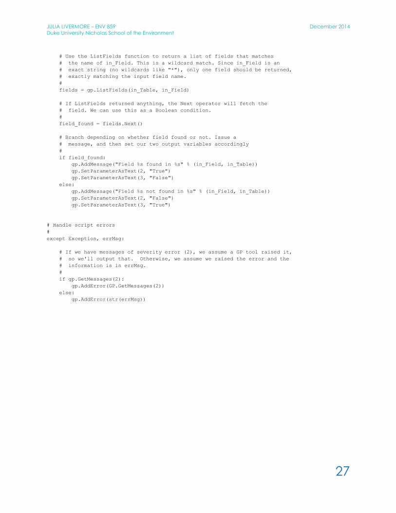
Script 3: Field Check Tool by ESRI

This tool is used in Step 2A, but is not included in any ArcGIS toolboxes. The ESRI-developed

python script has been added to the GAMs Toolbox as a new script, and is incorporated into

one of the models.

#**********************************************************************

# Description:

# Tests if a field exists and outputs two booleans:

# Exists - true if the field exists, false if it doesn't exist

# Not_Exists - true if the field doesn't exist, false if it does exist

# (the logical NOT of the first output).

#

# Arguments:

# 0 - Table name

# 1 - Field name

# 2 - Exists (boolean - see above)

# 3 - Not_Exists (boolean - see above)

#

# Created by: ESRI

#**********************************************************************

# Standard error handling - put everything in a try/except block

#

try:


import sys, string, os, arcgisscripting

# Create the Geoprocessor object

gp = arcgisscripting.create()

# Get input arguments - table name, field name

#

in_Table = gp.GetParameterAsText(0)

in_Field = gp.GetParameterAsText(1)

# First check that the table exists

#

if not gp.Exists(in_Table):

raise Exception, "Input table does not exist"



27

# Use the ListFields function to return a list of fields that matches

# the name of in_Field. This is a wildcard match. Since in_Field is an

# exact string (no wildcards like "*"), only one field should be returned,

# exactly matching the input field name.

#

fields = gp.ListFields(in_Table, in_Field)

# If ListFields returned anything, the Next operator will fetch the

# field. We can use this as a Boolean condition.

#

field_found = fields.Next()

# Branch depending on whether field found or not. Issue a

# message, and then set our two output variables accordingly

#

if field_found:

gp.AddMessage("Field %s found in %s" % (in_Field, in_Table))

gp.SetParameterAsText(2, "True")

gp.SetParameterAsText(3, "False")

else:

gp.AddMessage("Field %s not found in %s" % (in_Field, in_Table))

gp.SetParameterAsText(2, "False")

gp.SetParameterAsText(3, "True")

# Handle script errors

#

except Exception, errMsg:

# If we have messages of severity error (2), we assume a GP tool raised it,

# so we'll output that. Otherwise, we assume we raised the error and the

# information is in errMsg.

#

if gp.GetMessages(2):

gp.AddError(GP.GetMessages(2))

else:

gp.AddError(str(errMsg))

gams_toolbox_guide

Documents

general additive models

trawl data usage

data extraction

habitat of species

noaa trawl survey data

noaa nefsc trawl survey

species of fish

selected species