Gamma Rate Theory for Causal Rate Control in SourceCoding and Video Coding

Jun Xu and Dapeng Wu∗

Department of Electrical and Computer Engineering, University of Florida, Gainesville, Florida32611

Abstract

The rate distortion function in information theory provides performance bounds

for lossy source coding. However, it is not clear how to causally encode a Gaus-

sian sequence under rate constraints while achieving R-D optimality. This prob-

lem has significant implications in the design of rate control for video communi-

cation. To address this problem, we take distortion fluctuation into account and

develop a new theory, called gamma rate theory, to quantify the trade-off between

rate and distortion fluctuation. The gamma rate theory implies that, to evaluate the

performance of causal rate controls in source coding, the traditional R-D metric

needs to be replaced by a new GRD metric. The gamma rate theory identifies the

trade-off between quality fluctuation and bandwidth, which is not known previ-

ously. To validate the gamma rate theory, we design a rate control algorithm for

video coding; our experimental results demonstrate the utility of the gamma rate

theory in video coding.

Keywords: Causal rate control, rate distortion function, source coding, video

∗Please direct all correspondence to Prof. Dapeng Wu, University of Florida, Dept. of Electri-cal & Computer Engineering, P.O.Box 116130, Gainesville, FL 32611, USA. Tel. (352) 392-4954.Fax (352) 392-0044. Email: wu@ece.ufl.edu. Homepage: http://www.wu.ece.ufl.edu. This workwas supported in part by NSF ECCS-1002214, CNS-1116970, and NSFC 61228101.

Preprint submitted to Elsevier September 17, 2014

coding.

1. Introduction

In this paper, we consider the problem of causal rate control in source coding.

This problem has significant implications for the design of practical rate con-

trol schemes in video coding. In video coding, rate control is needed to achieve

user-specified bit-rate target while minimizing distortion. In video compression

for Digital Video Disc (DVD), the user-specified bit-rate target is applied to the

whole video sequence; e.g., a user may require that the entire compressed video

sequence be contained in a single DVD-4 disk of 5.32 Gigabytes. In the past ten

years, due to the rapid growth of streaming video over the Internet and wireless

networks, compression for streaming video has become a major topic of source

coding. The existing compression modules for streaming video usually use rate

control to adjust the compressed bit rate to the channel condition or channel ca-

pacity; i.e., in video compression for video communication or Internet television

(IPTV for short), the user-specified bit-rate target is applied to each video frame

or each second; e.g., a user may require that the compressed bit-rate be at most

300 kilo-bits per second (kb/s) to meet the channel capacity constraint.

To achieve optimal rate distortion performance under the user-specified bit-

rate budget, one needs to design a rate control scheme to determine how many

bits Ri is needed to compress the i-th frame (i = 1, 2, · · · , N , where N is the

total number of frames) in order to minimize the average distortion, which is av-

eraged over all the frames. Rate-distortion (R-D) theory provides the theoretical

foundation for lossy data compression [1][2][3][4] and rate control in video cod-

ing. It addresses the problem of minimizing the average distortion subject to a

2

compression data rate constraint. The R-D function provides a performance limit

for practical lossy data compression systems. If a non-causal rate control (which

has access to all the future frames) is used, the R-D-optimal rate control is in the

form of reverse water-filling for a Gaussian random sequence of finite length1 [5,

Page 314]. But the non-causal rate control that has access to all the future frames,

is not feasible for video communication and IPTV. For video communication and

IPTV, causal rate control or a nearly causal rate control that buffers a few frames,

is usually employed [6, 7, 8, 9, 10, 11, 12, 13, 14, 15, 16, 17, 18, 19]; however,

the existing rate control laws only consider performance in terms of rate and aver-

age distortion but do not consider distortion fluctuation over frames quantitatively

when designing algorithms, although variance of video quality (e.g. PSNR) is

a commonly used metric for comparisons.[20] claimed to consider video quality,

but only average PSNR was reported and no consistency measurement is reported.

From visual psychophysics [21], it is well known that large changes in distortion

over frames are much more annoying from a viewer’s perspective, compared to

the case with constant distortion (over frames) and the same average distortion

value. For this reason, it is desirable to design a rate control scheme that achieves

optimal performance in terms of rate, average distortion, and distortion fluctua-

tion. However, none of the existing works provides optimal performance bounds

for causal or nearly causal rate control in terms of rate, average distortion, and dis-

tortion fluctuation. To address this, we propose a new theory called gamma rate

theory, which provides optimal performance bounds for causal or nearly causal

rate control under the former mentioned three metrics.

1A Gaussian random sequence of length N is treated as an N -dimensional Gaussian random

vector.

3

The main contributions of this paper are 1) gamma rate theory, which serves as

the theoretical guide for rate control algorithm design, and 2) a new performance

metric for evaluating video coding algorithms, i.e., a triplet of {γD, R,D}, where

γD is the maximum distortion variation between two adjacent samples. The pro-

posed gamma rate theory includes 1) definition of a few new concepts such as the

gamma rate function and the rate gamma function, and 2) important properties of

the gamma rate function.

The rest of this paper is organized as follows. Section 2 formulates the prob-

lem. In Section 3, we present the gamma rate theory; i.e., define a few new

concepts needed in the gamma rate theory, and study important properties of the

gamma rate function. Section 4 presents a rate control algorithm for video cod-

ing, which is used to demonstrate the utility of the proposed gamma rate theory.

Section 5 shows simulation results to verify the gamma rate theory. Section 6

concludes the paper. Mathematical proofs are provided in Section 7.

2. Problem Formulation

In this section, we formulate the problems of non-causal and causal rate con-

trol in source coding.

We first define a few concepts as below.

Definition 1. {Xi}Ni=1 is said to be an independent Gaussian sequence if Xi (i =1, · · · , N ) are independent Gaussian random variables and Xi has fixed varianceσ2i (i = 1, · · · , N ) and zero mean.

Since this paper only considers Gaussian random variables, the distortion used

in this paper is quadratic distortion.

Definition 2. Let Ri denote the number of bits allocated to Xi; Ri ≥ 0 (i =1, · · · , N ). A rate allocation strategy R (specified by {Ri}Ni=1) for an independent

4

Gaussian sequence {Xi}Ni=1 is said to be R-D optimal if the resulting distortionfor Xi is Di(Ri) (i = 1, · · · , N ), where Di(Ri) is the distortion rate function ofXi.

Definition 3. A rate allocation strategy R (specified by {Ri}Ni=1) for an indepen-dent Gaussian sequence {Xi}Ni=1 is said to be causal under rate constraint R if

n∑i=1

Ri ≤ n×R, n = 1, · · · , N,

Ri ≥ 0, i = 1, · · · , N.

Otherwise, R is non-causal.

2.1. Non-causal Rate Control

We first begin with optimal non-causal rate control.

For an independent Gaussian sequence {Xi}Ni=1, an optimal non-causal rate

control problem can be formulated by

min{Ri}Ni=1

N∑i=1

Di(Ri) (1a)

s.t.N∑i=1

Ri = r (1b)

Ri ≥ 0 (i = 1, · · · , N) (1c)

where Di(Ri) is the distortion rate function of Xi (i = 1, · · · , N ), and r is the

total bit budget for N random variables {Xi}Ni=1. Denote {R∗i }Ni=1 the optimal

solution to (1). The resulting optimal non-causal rate allocation strategy Rnc is

specified by {R∗i }Ni=1.

Denote Dnc(r) the distortion rate function of {Xi}Ni=1, which can (roughly)

be regarded as the inverse function of the rate distortion function defined in [5,

Page 313]. Then, it is easy to show that Dnc(r) =∑N

i=1Di(R∗i ), i.e., at rate r, the

minimum distortion is∑N

i=1Di(R∗i ). So we have the following proposition.

5

Proposition 1. For an independent Gaussian sequence {Xi}Ni=1 with variances{σ2

i }Ni=1 and zero mean, its distortion rate function is given by

Dnc(r) =N∑i=1

σ2i e

−2Ri , (2)

where

Ri =

{12log

σ2i

λif λ < σ2

i

0 otherwise, (3)

where λ is chosen so that∑N

i=1Ri = r.

2.2. Causal Rate Control

For an independent Gaussian sequence {Xi}Ni=1, an optimal causal rate control

problem can be formulated as below.

Upon the arrival of Xi (i = 1, · · · , N ), solve the following problem

minRi

Di(Ri) (4a)

s.t. Ri ≤ n×R−i−1∑j=1

R∗j (4b)

Ri ≥ 0 (4c)

where R∗j is the solution to (4) in previous steps (i.e., j < i).

2.3. Causal Rate Control with Smooth Distortion Change

Since distortion fluctuations will affect perceptual video quality, to study this

effect, we introduce constraints on distortion fluctuations.

6

For an independent Gaussian sequence {Xi}Ni=1, an optimal causal rate control

problem with constraints on distortion fluctuations can be formulated by

min{Ri}Ni=1

N∑i=1

Di(Ri) (5a)

s.t.n∑

i=1

Ri ≤ n×R (n = 1, · · · , N), (5b)

Ri ≥ 0 (n = 1, · · · , N), (5c)

|∆Di| ≤ γD (i = 1, · · · , N − 1), (5d)

where ∆Di = Di+1 − Di (i = 1, · · · , N − 1), and γD is the maximal tolerable

fluctuation in distortion.

Taking the constraint on distortion fluctuations into account, we will explore

the relationship between the rate R (given in (5b)) and the maximum change of

distortion γD (given in (5d)) and derive a series of theorems, which form the foun-

dation for what we call Gamma Rate Theory. The key principle of Gamma Rate

Theory is that reducing (increasing, respectively) the rate will result in increased

(reduced, respectively) distortion fluctuation, or vice versa. The gamma rate the-

ory tells that there is a fundamental tradeoff between the rate and the distortion

fluctuation. In the next section, we present our gamma rate theory.

3. Gamma Rate Theory

We first define a few concepts as below.

Definition 4. An independent Gaussian sequence {Xi}Ni=1 is said to be control-lable w.r.t. R and γD (R ≥ 0 and γD ≥ 0) if there exists a causal R-D optimalrate allocation strategy R such that |∆Di(R)| < γD (∀i), where

∆Di(R) = Di+1(Ri+1)−Di(Ri), i = 1, · · · , N − 1,

7

n∑i=1

Ri ≤ nR, n = 1, · · · , N,

Ri ≥ 0, i = 1, · · · , N.

Definition 5. (R, γD) is said to be controllable w.r.t. an independent Gaussiansequence {Xi}Ni=1 if {Xi}Ni=1 is controllable w.r.t. γD and R.

Definition 6. For an independent Gaussian sequence {Xi}Ni=1, its controllableregion in R–γD plane is the closure of the set of all controllable (R, γD) pairs.Denote the controllable region by C{Xi}.

Definition 7. The gamma rate function Γ(R) of {Xi}Ni=1 is the infimum of all γDsuch that (R, γD) is in the controllable region of {Xi}Ni=1 for a given R.

Definition 8. The rate gamma function R(γD) of {Xi}Ni=1 is the infimum of all Rsuch that (R, γD) is in the controllable region of {Xi}Ni=1 for a given γD.

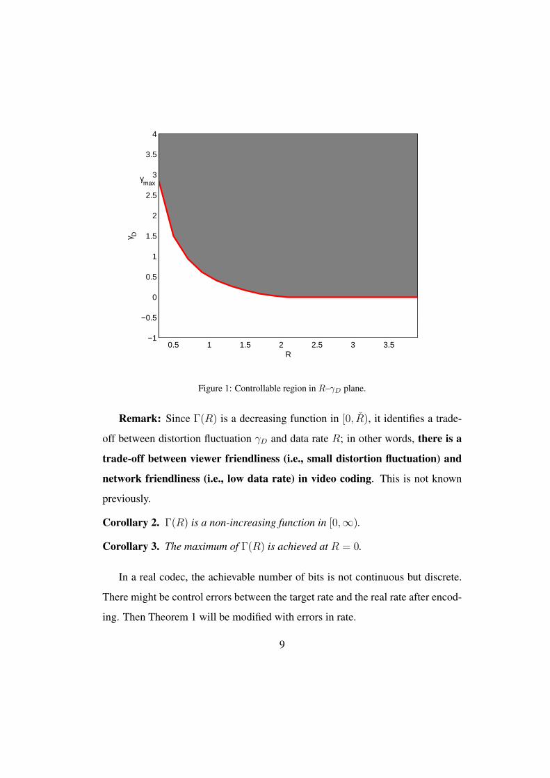
Remark: Just like a distortion rate function, there exists a gamma rate func-

tion that serves as the boundary of the controllable region of {Xi}Ni=1 as shown in

Figure 1.

Theorem 1. Given an independent Gaussian sequence {Xi}Ni=1 with variances{σ2

i }Ni=1, denote the minimum of {σ2i }Ni=1 by σ2

min = mini∈{1,··· ,N} σ2i . The gamma

rate function Γ(R) has the following properties:1) Γ(R) ≥ 0.2) Γ(R) is a decreasing function for R ∈ [0, R), where

R = minR∈{R:Γ(R)=0}

R; (6)

3)

R = maxn=1,··· ,N

1

2log2

n√∏n

i=1 σ2i

σ2min

(7)

4) Γ(R) = 0 for R ∈ [R,∞).

8

0.5 1 1.5 2 2.5 3 3.5−1

−0.5

0

0.5

1

1.5

2

2.5

3

3.5

4

R

γ D

γmax

Figure 1: Controllable region in R–γD plane.

Remark: Since Γ(R) is a decreasing function in [0, R), it identifies a trade-

off between distortion fluctuation γD and data rate R; in other words, there is a

trade-off between viewer friendliness (i.e., small distortion fluctuation) and

network friendliness (i.e., low data rate) in video coding. This is not known

previously.

Corollary 2. Γ(R) is a non-increasing function in [0,∞).

Corollary 3. The maximum of Γ(R) is achieved at R = 0.

In a real codec, the achievable number of bits is not continuous but discrete.

There might be control errors between the target rate and the real rate after encod-

ing. Then Theorem 1 will be modified with errors in rate.

9

Theorem 4. An independent Gaussian sequence {Xi}Ni=1 is encoded subject tocausal rate constraints

∑ni=1Ri ≤ nR (∀n ∈ {1, 2, · · · , N}) and there are ran-

dom values {En, n = 1, 2, · · · , N} such that R1 + E1 ≤ R and Rn + En ≤nR −

∑n−1i=1 Ri (∀n ∈ {2, · · · , N}). {En, n = 1, 2, · · · , N} are uniformly dis-

tributed between −Emax and Emax, where 0 < Emax < R. The following proper-ties still hold.

1) Γ(R) ≥ 0.2) Γ(R) is a decreasing function for R ∈ [0, R), where R = minR∈{R:Γ(R)=0} R3) Γ(R) = 0 for R ∈ [R,∞).

In practical video systems, there is always a buffer available for rate control

algorithms. The buffer enables the current frame to borrow bit budget from future

frames. Intuitively, we may think that the buffer will improve the performance of

Γ(R). However, a buffer does not help here.

Theorem 5. An independent Gaussian sequence {Xi}Ni=1 is encoded by a R-Doptimal rate allocation strategy {Ri}Ni=1 with a buffer, which is

∑ni=1 Ri ≤ nR +

B, where B is the buffer size and n ∈ {1, · · · , N}. The buffer will not changeΓ(R).

4. Rate Control in Video Coding

To demonstrate the utility of our proposed gamma rate theory in real-world

problems, we use rate control in video coding as an example. In this section,

we show our design of a new rate control scheme. In Section 5, we will show

experimental results to illustrate the usefulness of the gamma rate theory.

4.1. Problem Formulation

To present our rate control algorithm, we first begin with a scenario of encod-

ing two video frames using predictive coding (P-frame). Suppose a video codec

has finished encoding the (n − 1)th frame. Let Rt denote the total bit budget for

the nth and (n+1)th frames. The rate allocation for the two frames is ηRt for the

10

nth frame and (1−η)Rt for the (n+1)th frame, where η ∈ [0, 1] is a bit-allocation

parameter. Then the problem (1) is reduced to

minη

Dn(ηRt) +Dn+1((1− η)Rt) (8)

where Dn(R) is the rate-distortion function for the nth frame.

We can partition a video frame into SKIP macroblocks (MBs) and non-SKIP

MBs. A SKIP MB consumes negligible number of bits from the bit budget since

only one flag to indicate SKIP MB and no other information for a SKIP MB will

be sent to the decoder. Then the distortion of the nth frame is

Dn(ηRt) = ρTnDSn + (1− ρTn )D

Nn (ηRt), (9)

where ρTn is the percentage of SKIP MBs, DSn is the average distortion of a SKIP

MB, and DNn (ηRt) is the average distortion of a non-SKIP MB. The reconstructed

pixel values in a SKIP MB are exactly the same as the corresponding MB in

the previous frame. Hence, considering the high similarity between two adjacent

frames, we assume that DSn+1 ≈ Dn(ηRt) and DS

n is independent of η and Rt.

Then the goal of our rate control algorithm is to minimize the total distortion of

two frames, given by

D(Rt) = Dn(ηRt) +Dn+1((1− η)Rt) (10)

= ρTnDSn + (1− ρTn )D

Nn (ηRt) + ρTn+1(ρ

TnD

Sn + (1− ρTn )D

Nn (ηRt))(11)

+ (1− ρTn+1)DNn+1((1− η)Rt).

Then the problem becomes

minη

ρTnDSn+(1−ρTn )D

Nn (ηRt)+ρTn+1(ρ

TnD

Sn+(1−ρTn )D

Nn (ηRt))+(1−ρTn+1)D

Nn+1((1−η)Rt).

(12)

11

Eq. (12) can be easily extended to K frames (K > 2) by introducing (K − 1)

bit-allocation parameters (similar to η).

A closed form solution to (12) can be obtained if the closed form of the rate-

distortion functions in (12) are given. Different rate-distortion functions will yield

different solutions for (12). In video coding systems, prediction residual errors

are usually modeled by Gaussian, or Laplacian [22], or Cauchy distribution [23].

In the next subsection, we will derive a closed form solution to (12) based on

Gaussian distribution as a model for prediction residual errors.

4.2. R-D Model

Assume that the prediction residual error follows a Gaussian distribution. Then

its rate-distortion function is given by

D = σ2 · 2−2R (13)

where σ2 is the variance of the residual error, and D is mean squared error (MSE).

For the nth and (n+1)th frame, all the bits are used for encoding non-SKIP MBs.

So we have

DNn (ηRt) = σ2

n · 2−2ηRt (14)

DNn+1((1− η)Rt) = σ2

n+1 · 2−2(1−η)Rt (15)

where σ2n and σ2

n+1 are the variances of a non-SKIP MB of the nth and (n + 1)th

frame, respectively. Then Eq. (12) becomes

minη

ρTnDSn + (1− ρTn )σ

2n2

−2ηRt + ρTn+1(ρTnD

Sn + (1− ρTn )σ

2n2

−2ηRt) + (1− ρTn+1)σ2n+12

−2(1−η)Rt(16)

Letting ∂D/∂η = 0 gives the optimal solution η∗ as below

η∗ =1

2+

1

4Rt

[log2((1− ρTn )(1 + ρTn+1)

1− ρTn+1

) + log2(σ2n

σ2n+1

)]. (17)

12

Once η∗ is obtained, the bit budget for the nth frame and the (n + 1)th frame

is η∗Rt and (1 − η∗)Rt, respectively. In the next subsection, we determine the

quantization step size for quantizing residual errors, given a bit budget for a video

frame.

4.3. R-Q Model

To determine the quantization step size for quantizing residual errors, we need

a R-Q model to map a bit budget R to quantization step size Q. Since 1) our R-Q

model only describes the relationship between the bits for encoding residual errors

and Q, and 2) the bit budget of a frame includes texture bits for encoding residual

errors and header bits for encoding motion vectors and overheads, hence we need

to estimate the bit budget for encoding residual errors. A simple method is to use

the number of header bits in the previous frame as a prediction of the number of

header bits in the current frame; then the bit budget for residual errors is simply

the bit budget of the frame minus the predicted number of header bits.

An quadratic R-Q model [24] is given by

R = x1MAD

Q+ x2

MAD

Q2(18)

where x1 and x2 are model parameters, MAD denotes the mean absolute dif-

ference between the original pixel value and its reconstructed one, and Q is the

quantization step size. The MAD of the current frame can be predicted by the

MAD of the previous frames, i.e.,

˜MADn = α1 ∗MADn−1 + α2 (19)

where MADn−1 is the actual MAD of the (n − 1)th frame, and α1 and α2 are

model parameters.

13

Using (19), we can obtain an estimate ˜MADn. Plugging this estimated MAD

into (18), we can obtain the quantization step size Q since the bit budget R for

residual error and x1 and x2 are known. Using the obtained Q to quantize the

residual errors, we obtain the coded bits for the current frame. After finishing

encoding the current frame, we use the least-squares method to estimate the model

parameters x1, x2, α1 and α2 of the current frame, and use these updated model

parameters for encoding the next frame. This procedure is conducted iteratively.

4.4. Rate Control Algorithm

In this subsection, we describe our rate control algorithm. For each frame, our

rate control algorithm operates as follows.

1. Initialize the bit budget for the frame.

Allocate a certain bit budget to the current frame R′t according to the ap-

proach in JVT-G012 [25]. Then Rt = 2R′t since Rt is the bit budget for two

frames. Initialize model parameters to initial values.

2. Calculate the target bit budget.

Compute (17) to obtain η∗, where σn can be estimated by the statistics in

the previous frame, and ρT can be specified by a user or automatically de-

termined by (20). Then the target bit budget for the current frame is η∗Rt.

3. Determine the quantization step size Q.

The bit budget for residual errors is equal to η∗Rt minus the predicted num-

ber of header bits. Use (19) to obtain an estimate ˜MADn. Plug this esti-

mated MAD into (18) to obtain the quantization step size Q.

4. Update of model parameters.

Use the least-squares method to estimate the model parameters of the cur-

rent frame, given the encoded data of the current frame and the previous

14

frames.

We implement the above rate control algorithm in JM15.1 [26].

In the above algorithm, ρT can be specified by a user. ρT can also be automat-

ically determined by the following procedure.

We estimate ρTn by a linear model

ρTn = β1ρTn−1 + β2 (20)

where ρTn−1 is the actual ρT of (n−1)th frame and β1 and β2 are model parameters,

which are updated after a frame is encoded. ρTn+1 is estimated by (20) with (n+1)

replacing n and ρTn replacing the actual ρTn .

5. Simulation Results

In this section, we use simulations to validate the gamma rate theory presented

in Section 3. This section is organized as below: Section 5.1 presents simulation

results for synthetic data, and Section 5.2 presents simulation results for real-

world data.

5.1. Simulation with Synthetic Data

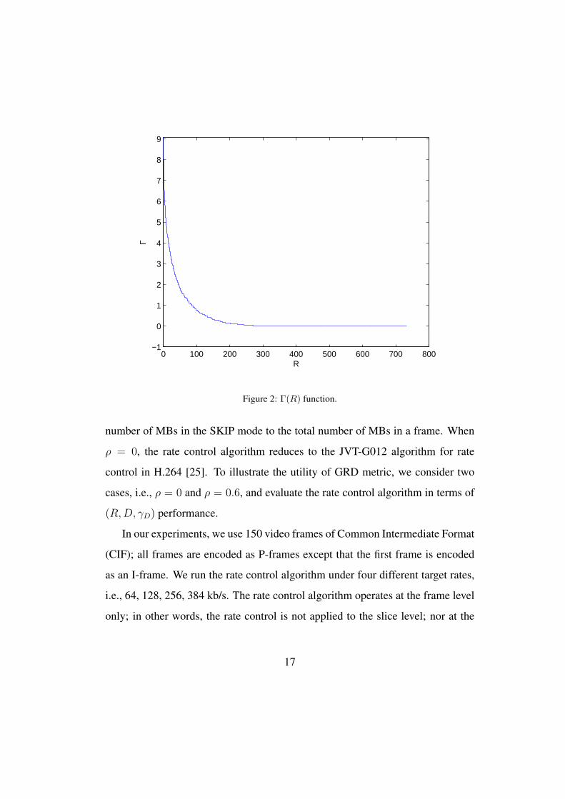
In this section, we use synthetic data to validate that Γ(R) function is indeed a

non-increasing function of R. To achieve this, we generate N samples, denoted by

{σ2i , i = 1, ..., N}. Specifically, each σ2

i (i = 1, ..., N ) follows the same uniform

distribution whose support is [0, σ2max], where σ2

max is a user-specified parameter.

In this simulation, we choose N = 100. Using Definition 7, we can compute

the gamma rate function Γ(R) of independent Gaussian sequence {Xi}Ni=1 with

zero means and variances σ2i (i = 1, ..., N). Figure 2 shows the resulting Γ(R).

15

As shown in the figure, the Γ(R) function obtained from the simulation has the

following properties.

1) Γ(R) ≥ 0.

2) Γ(R) is a decreasing function for R ∈ [0, R), where

R = minR∈{R:Γ(R)=0}

R. (21)

From Figure 2, we observe that R = 372, which is obtained from simulation.

3) Given {σ2i , i = 1, ..., N}, we can compute

R = maxn=1,··· ,N

1

2log2

n√∏n

i=1 σ2i

σ2min

= 375. (22)

Hence the value of R obtained from the simulation (which is 372) is very close to

the theoretical value of R (which is 375). This validates the correctness of Eq. (7).

4) Γ(R) = 0 for R ∈ [R,∞).

The above observations validate Theorem 1.

5.2. Simulation with Real-World Data

In this section, we would like to show the importance of the proposed Gamma

Rate Distortion (GRD) metric in real-world applications. We use rate control in

video coding as an example. Based on the gamma rate theory, conventional per-

formance measures, i.e., average rate and average distortion, are not sufficient to

quantify the overall performance of a rate control algorithm in video coding; in-

stead, we need to use the triplet (R,D, γD) to quantify the overall performance,

where R denotes the average rate, D denotes the average distortion, and γD de-

notes the maximum distortion fluctuation.

To show this, we implement the rate control algorithm described in Section 4

on reference software JM15.1 of H.264 [26]. Let ρ denote the percentage of the

16

0 100 200 300 400 500 600 700 800−1

0

1

2

3

4

5

6

7

8

9

R

Γ

Figure 2: Γ(R) function.

number of MBs in the SKIP mode to the total number of MBs in a frame. When

ρ = 0, the rate control algorithm reduces to the JVT-G012 algorithm for rate

control in H.264 [25]. To illustrate the utility of GRD metric, we consider two

cases, i.e., ρ = 0 and ρ = 0.6, and evaluate the rate control algorithm in terms of

(R,D, γD) performance.

In our experiments, we use 150 video frames of Common Intermediate Format

(CIF); all frames are encoded as P-frames except that the first frame is encoded

as an I-frame. We run the rate control algorithm under four different target rates,

i.e., 64, 128, 256, 384 kb/s. The rate control algorithm operates at the frame level

only; in other words, the rate control is not applied to the slice level; nor at the

17

MB level. The average rate difference between the two cases ρ = 0.6 and ρ = 0

under the same distortion is calculated via the method proposed in Ref. [27]. The

normalized average rate difference is defined by (r0.6 − r0)/r0 where r0.6 and r0

denote the rate of the coded bit-stream for ρ = 0.6 and ρ = 0 (under the same

distortion), respectively. The γD difference is equal to γD for ρ = 0.6 minus γD

for ρ = 0.

Table 1 shows target bit rate in unit of kb/s, actual average bit rate in kb/s,

average distortion in terms of peak signal to noise ratio (PSNR) in dB, normalized

average rate difference under the same distortion, and γD difference in dB, for

four widely-used test video sequences, namely, hall-monitor, paris, news, and

waterfall.

From Table 1, we observe that the rate control scheme with ρ = 0.6 achieves

bit saving (i.e., using less number of bits while achieving the same distortion, as

shown by negative values in the column of normalized average rate difference in

Table 1), compared to the rate control scheme with ρ = 0. This is mainly due

to the R-D optimization in (12). If we use conventional performance measures,

i.e., average rate and average distortion, we would declare the rate control scheme

with ρ = 0.6 is better than the rate control scheme with ρ = 0 in R-D sense, since

the former uses less number of bits on average under the same average distortion

(PSNR). However, this bit saving is obtained at a cost of larger fluctuation in dis-

tortion, as shown by positive values in the column of γD difference in Table 1.

A larger fluctuation in distortion is annoying to a viewer. Hence, conventional

performance measures, i.e., average rate and average distortion, are not sufficient

to quantify the overall performance of a rate control algorithm in video coding.

Based on the gamma rate theory, we advocate the use of triplet (R,D, γD) to

18

quantify the performance of a video codec. Furthermore, this experimental re-

sult also validates that there is a tradeoff between distortion fluctuation γD and

data rate R; in other words, there is a trade-off between viewer friendliness (i.e.,

small distortion fluctuation) and network friendliness (i.e., low data rate) in video

coding. This is not known previously.

6. Conclusion

In this paper, we consider the problem of causal rate control in source coding

including video coding. This problem is significant for the design of practical rate

control schemes in video coding. To address this problem, we consider distortion

fluctuation in our problem formulation and develop a new theory, called gamma

rate theory, to quantify the trade-off between rate and distortion fluctuation. Based

on the gamma rate theory, conventional performance measures, i.e., average rate

and average distortion, are not sufficient to quantify the performance of a rate con-

trol algorithm in video coding; instead, we advocate the use of triplet (R,D, γD)

to quantify the performance of a video codec, where R denotes the average rate,

D denotes the average distortion, and γD denotes the maximum distortion fluctu-

ation. In addition, our gamma rate theory identifies the trade-off between viewer

friendliness (i.e., smooth video quality over time) and network friendliness (i.e.,

low bit rate) in video coding, which is not known previously. To validate the

gamma rate theory, we design a rate control algorithm for video coding. Our sim-

ulation and experimental results validate the gamma rate theory and demonstrate

the utility of the gamma rate theory in video coding.

19

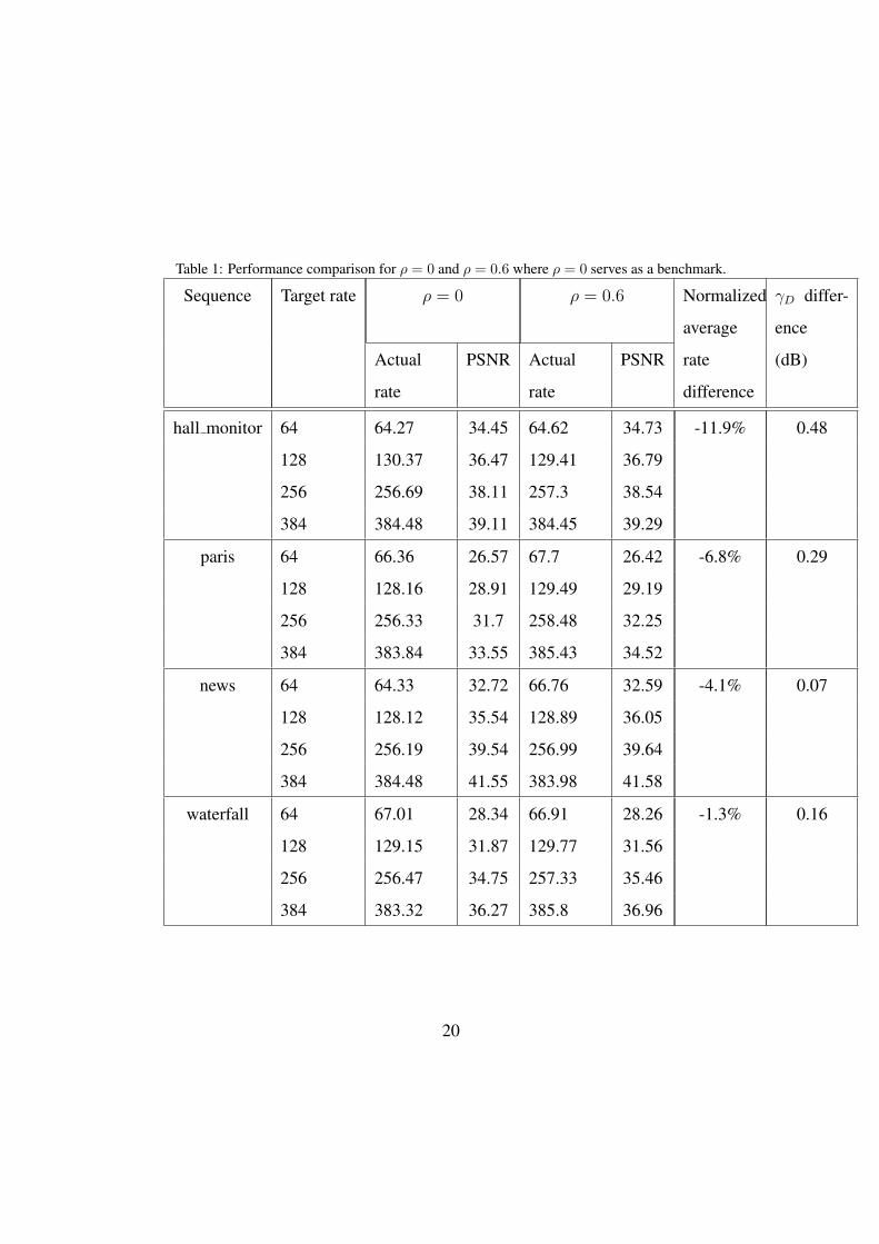
Table 1: Performance comparison for ρ = 0 and ρ = 0.6 where ρ = 0 serves as a benchmark.

Sequence Target rate ρ = 0 ρ = 0.6 Normalized

average

γD differ-

ence

Actual

rate

PSNR Actual

rate

PSNR rate

difference

(dB)

hall monitor 64 64.27 34.45 64.62 34.73 -11.9% 0.48

128 130.37 36.47 129.41 36.79

256 256.69 38.11 257.3 38.54

384 384.48 39.11 384.45 39.29

paris 64 66.36 26.57 67.7 26.42 -6.8% 0.29

128 128.16 28.91 129.49 29.19

256 256.33 31.7 258.48 32.25

384 383.84 33.55 385.43 34.52

news 64 64.33 32.72 66.76 32.59 -4.1% 0.07

128 128.12 35.54 128.89 36.05

256 256.19 39.54 256.99 39.64

384 384.48 41.55 383.98 41.58

waterfall 64 67.01 28.34 66.91 28.26 -1.3% 0.16

128 129.15 31.87 129.77 31.56

256 256.47 34.75 257.33 35.46

384 383.32 36.27 385.8 36.96

20

7. Appendix

7.1. Proof of Proposition 1Proof 1. Since the distortion rate function of {Xi}Ni=1 can be obtained by solving(1), using Lagrange multipliers, we construct the functional

J(R1, R2, · · · , RN) =N∑i=1

(σ2i e

−2Ri) + λ′

(N∑i=1

Ri

). (23)

Differentiating (23) with respect to Ri and setting it equal to zero, we have

∂J

∂Ri

= −2σ2i e

−2Ri + λ′ = 0. (24)

Let λ = λ′/2. From (24), we have

λ = σ2i e

−2Ri ∀i. (25)

Hence the optimum allocation of r bits to code {Xi}Ni=1 results in the same dis-tortion for all random variables {Xi}Ni=1, if λ in (25) is less than the minimum of{σ2

i }Ni=1. If λ in (25) is not less than the minimum of {σ2i }Ni=1, we use the Karush-

Kuhn-Tucker conditions to find the minimum in (23). The Karush-Kuhn-Tuckerconditions yield

∂J

∂Ri

= −2σ2i e

−2Ri + λ′, (26)

where λ′ is chosen so that∑N

i=1Ri = r and

∂J∂Ri

= 0 if λ′ < 2σ2i ,

∂J∂Ri

≤ 0 if λ′ ≥ 2σ2i .

(27)

The conditions ∂J∂Ri

≤ 0 and λ′ ≥ 2σ2i imply that Ri ≤ 0; since data rate Ri has

to be non-negative, we have Ri = 0 for λ ≥ σ2i . For λ′ < 2σ2

i , ∂J∂Ri

= 0 implies

λ = σ2i e

−2Ri , i.e., Ri =12log

σ2i

λ. This completes the proof.

21

7.2. Proof of Theorem 1Proof 2. Γ(R) is defined by

Γ(R) = maxi∈{1,··· ,N−1}

|Di+1(Ri+1)−Di(Ri)| (28)

1) From (28), it is obvious that Γ(R) ≥ 0.2) Now we prove that Γ(R) is a decreasing function for R ∈ [0, R), where

R = minR∈{R:Γ(R)=0}R.For two arbitrary points R1 and R2 in [0, R). Without loss of generality, as-

sume R1 < R2. In case there is only one source (say, source k) achieving themaximum value of ∆Di, i.e., k = argmaxi∈{1,··· ,N−1} |∆Di|, we let R1 = R1 + ϵ,where ϵ > 0 and ϵ is so small that ϵ bits can only be used to reduce |∆Dk|,while the resulting |∆Dk| under R1 is still the maximum among {|∆Di|} un-der R1. So Γ(R1) = |∆Dk| since |∆Dk| is the maximum among {|∆Di|}; and|∆Dk| < |∆Dk| since |∆Dk| is reduced to |Dk| due to ϵ bits. Since Γ(R1) =|∆Dk| > |∆Dk| = Γ(R1), we have Γ(R1) > Γ(R1).

In case there are L sources achieving the maximum value of ∆Di, i.e., kj =argmaxi∈{1,··· ,N−1} |∆Di| (j = 1, · · · , L), we let R1 = R1 + ϵ, where ϵ > 0 andϵ is so small that there exist {ϵj}Lj=1 (

∑Lj=1 ϵj = ϵ) and a bit allocation strategy

that guarantee that ϵj bits (j = 1, · · · , L) can only be used to reduce |∆Dkj |,while the resulting |∆Dkj | under R1 is still the maximum among |∆Di| under R1;in other words, the set of sources achieving the maximum value, i.e., I = {i∗ :i∗ = argmaxi∈{1,··· ,N−1} |Di|}, contains the L sources (sources {kj}Lj=1) and thecardinality |I| ≥ L; in other words, there could be new sources achieving themaximum value. Since Γ(R1) = |∆Dkj | > |∆Dkj | = Γ(R1), we have Γ(R1) >

Γ(R1).Following the same proof for Γ(R1) > Γ(R1), for a sufficiently large M , there

exist {Ri}Mi=2 and {εi}Mi=1 such that Γ(R1) > Γ(R1) > Γ(R2) > · · · > Γ(RM) >Γ(R2), where Ri+1 = Ri + εi (i = 1, · · · ,M − 1) and R2 = RM + εM .

Since for two arbitrary points R1 and R2 in [0, R) and R1 < R2, we haveΓ(R1) > Γ(R2), hence Γ(R) is a decreasing function in [0, R).

3) Now we prove that R = maxn=1,··· ,N12log2

n√∏n

i=1 σ2i

σ2min

and Γ(R) = 0, where

R = minR∈{R:Γ(R)=0} R. There are two steps to finish the proof. In the first step,we prove there exists R such that Γ(R) = 0. In the second step, we prove that

R = maxn=1,··· ,N12log2

n√∏n

i=1 σ2i

σ2min

, where R = minR∈{R:Γ(R)=0} R and Γ(R) = 0.

22

Firstly, let R = maxn=1,··· ,N12log2

n√∏n

i=1 σ2i

σ2min

. Then we have

R ≥ 1

2log2

n√∏n

i=1 σ2i

σ2min

, n = {1, · · · , N} (29)

Then

σ2min ≥ 2−2R n

√√√√ n∏i=1

σ2i , n = {1, · · · , N} (30)

So there exists a D such that

σ2min ≥ D ≥ 2−2R n

√√√√ n∏i=1

σ2i , n = {1, · · · , N} (31)

Therefore, we have

1

2log2

∏ni=1 σ

2i

Dn≤ nR, n = {1, · · · , N} (32)

Then we haven∑

i=1

(1

2log2

σ2i

D) ≤ nR, n = {1, · · · , N} (33)

Then we can find a rate allocation strategy R with {Ri = 12log2

σ2i

D}Ni=1. This

strategy is a causal and R-D optimal strategy verified by Eq. (33). {Ri =12log2

σ2i

D}Ni=1

implies consistent distortion for all sources, which is Di = D, i ∈ {1, · · · , N}.Then ∆Di(R) = 0, i ∈ {1, · · · , N−1}. So we have Γ(R) = maxi=1,··· ,N−1 |∆Di(R)| =

0. So there exists R such that Γ(R) = 0. Here R = maxn=1,··· ,N12log2

n√∏n

i=1 σ2i

σ2min

.

Secondly, we prove that R = maxn=1,··· ,N12log2

n√∏n

i=1 σ2i

σ2min

, where R = minR∈{R:Γ(R)=0}R

and Γ(R) = 0. We prove this by contradiction.

Assume R < maxn=1,··· ,N12log2

n√∏n

i=1 σ2i

σ2min

. Then there must exist a k ∈{1, · · · , N} such that

R <1

2log2

k

√∏ki=1 σ

2i

σ2min

(34)

⇔ σ2min < 2−2R k

√√√√ k∏i=1

σ2i (35)

23

Since Γ(R) = 0, then there must exist a causal rate allocation strategy R withrates {Ri}Ni=1 and distortions {Di}Ni=1 for R such that maxi=1,··· ,N−1 |∆Di(R)| =0. Then |∆Di| = 0. So |Di+1 − Di| = 0, i = 1, · · · , N − 1 and denoteD = Di, i = {1, · · · , N}. The causal strategy R will have

n∑i=1

(1

2log2

σ2i

D) ≤ nR n = {1, · · · , N} (36)

Rate distortion function of Gaussian sources implies that

Di ≤ σ2i i = {1, · · · , N} (37)

Then we haveD ≤ σ2

i i = {1, · · · , N} (38)

Then we haveD ≤ σ2

min (39)

Combining Eq. (36) and Eq. (39), we have

σ2min ≥ D ≥ 2−2R n

√√√√ n∏i=1

σ2i , n = {1, · · · , N} (40)

Eq. (40) conflicts with Eq. (35), so the assumption of R < maxn=1,··· ,N12log2

n√∏n

i=1 σ2i

σ2min

is not correct. Then we must have R ≥ maxn=1,··· ,N12log2

n√∏n

i=1 σ2i

σ2min

. Since

we have proven that Γ(R) = 0 for R = maxn=1,··· ,N12log2

n√∏n

i=1 σ2i

σ2min

and R =

minR∈{R:Γ(R)=0} R, we have R = maxn=1,··· ,N12log2

n√∏n

i=1 σ2i

σ2min

.

4) Finally, we prove Γ(R) = 0 for R ∈ (R,∞).Assume a causal rate allocation strategy R for R with rates {Ri}Ni=1 and dis-

tortions {Di}Ni=1, where D = Di i ∈ {1, · · · , N}. For an arbitrary R∗ = R+ ϵwhere ϵ > 0, we can find a rate allocation strategy R∗ with rates {R∗

i }Ni=1 anddistortions {D∗

i }Ni=1. When changing from R to R∗ , we add ϵ bits to each source.That is R∗

i = Ri + ϵ for i ∈ {1, · · · , N}.Thus

n∑i=1

R∗i =

n∑i=1

(Ri + ϵ) =n∑

i=1

Ri + nϵ (41)

24

Since∑n

i=1Ri ≤ nR, we have

n∑i=1

R∗i ≤ n(R + ϵ) = nR∗ (42)

So R∗ is causal and R-D optimal rate allocation strategy.The distortion of R∗ are

D∗i = σ2

i 2−2R∗

i = σ2i 2

−2(Ri+ϵ) = 2−2ϵDi (43)

Since D = Di i ∈ {1, · · · , N}, we have

D∗i = 2−2ϵD, i ∈ {1, · · · , N} (44)

Then∆Di(R∗) = D∗

i+1 −D∗i = 0, i ∈ {1, · · · , N − 1} (45)

SoΓ(R∗) = max

i∈{1,··· ,N−1}|∆Di(R∗)| = 0 (46)

Since Γ(R∗) = 0 for an arbitrary R∗ > R, we proved Γ(R) = 0 in R ∈(R,∞).

7.3. Proof of Corollary 2Proof 3. According to the properties 2) and 4) in Theorem 1, Γ(R) is a non-increasing function in [0,∞). Specifically, Γ(R) is a decreasing function for R ∈[0, R), where Γ(R) = 0; and Γ(R) = 0 for R ∈ [R,∞).

7.4. Proof of Corollary 3Proof 4. According to the properties 2) and 4) in Theorem 1, Γ(R) is a non-increasing function in [0,∞). Specifically, Γ(R) is a decreasing function for R ∈[0, R), where Γ(R) = 0; and Γ(R) = 0 for R ∈ [R,∞).

25

7.5. Proof of Theorem 4Proof 5. To prove the gamma rate theory with control errors, we try to con-vert the control errors to the variation of sources. Given {Xi}Ni=1 and {Ei, i =1, 2, · · · , N}, there exists an equivalent source {Xi}Ni=1 with variances {σ2

i },which satisfies

Ri + Ei =1

2log2

σ2i

Di = 1, · · · , N (47)

For a fixed distortion D, the equivalent source has relationship with the originalsource as

σi = 2Eiσi (48)

Then the proof reduces to the proof of Theorem 1 with modified sources {Xi}Ni=1.As long as the original source {Xi}Ni=1 is controllable, Theorem 4 is correct.

7.6. Proof of Theorem 5Proof 6. We rewrite the strategy as

n∑i=1

Ri ≤ n(R +B

n) n ∈ {1, · · · , N} (49)

When n → ∞, Bn

→ 0. The strategy with buffer reduces to a bufferless causalstrategy asymptotically. Then Γ(R) of the strategy with buffers stays the same asthe bufferless strategy.

References

[1] C. Shannon, A mathematical theory of communication, Bell System Techni-

cal Journal 27 (1948) 379–423.

[2] C. Shannon, Coding theorems for a discrete source with a fidelity criterion,

Information and decision processes (1960) 93–126.

[3] T. Berger, Rate distortion theory, Prentice-Hall, Englewood Cliffs, NJ, 1971.

[4] R. Gray, Source coding theory, Springer, 1990.

26

[5] T. Cover, J. Thomas, Elements of information theory, 2nd Edition, Wiley,

Hoboken, New Jersey, 2006.

[6] G. Sullivan, T. Wiegand, Rate-distortion optimization for video compres-

sion, IEEE Signal Processing Magazine 15 (6) (1998) 74–90.

[7] A. Ortega, K. Ramchandran, Rate-distortion methods for image and video

compression, IEEE Signal Processing Magazine 15 (6) (1998) 23–50.

[8] D. Wu, Y. Hou, W. Zhu, H. Lee, T. Chiang, Y. Zhang, H. Chao, On end-

to-end architecture for transporting MPEG-4 video over the Internet, IEEE

Transactions on Circuits and Systems for Video Technology 10 (6) (2000)

923–941.

[9] D. Wu, Y. Hou, Y. Zhang, Transporting real-time video over the Internet:

Challenges and approaches, Proceedings of the IEEE 88 (12) (2000) 1855–

1875.

[10] D. Wu, Y. Hou, W. Zhu, Y. Zhang, J. Peha, Streaming video over the Internet:

approaches and directions, IEEE Transactions on Circuits and Systems for

Video Technology 11 (3) (2001) 282–300.

[11] J. Cai, Z. He, C. Chen, A novel frame-level bit allocation based on two-

pass video encoding for low bit rate video streaming applications, Journal of

Visual Communication and Image Representations 17 (4) (2006) 783–798.

[12] S. Zhou, J. Li, J. Fei, Y. Zhang, Improvement on rate-distortion performance

of H.264 rate control in low bit rate, IEEE Transactions on Circuits and

Systems for Video Technology 17 (8) (2007) 996–1006.

27

[13] M. Jiang, N. Ling, Low-delay rate control for real-time H.264/AVC video

coding, IEEE Transactions on Multimedia 8 (3) (2006) 467–477.

[14] C. Huang, C. Lin, A novel 4-D perceptual quantization modeling for H.264

bitrate control, IEEE Transactions on Multimedia 9 (6) (2007) 1113–1124.

[15] Z. Chen, K. Ngan, Towards rate-distortion tradeoff in real-time color video

coding, IEEE Transactions on Circuits and Systems for Video Technology

17 (2) (2007) 158–167.

[16] D.-K. Kwon, M.-Y. Shen, C. Kuo, Rate control for H.264 video with en-

hanced rate and distortion models, IEEE Transactions on Circuits and Sys-

tems for Video Technology 17 (5) (2007) 517–529.

[17] J. Dong, N. Ling, A context-adaptive prediction scheme for parameter esti-

mation in h. 264/avc macroblock layer rate control, Circuits and Systems for

Video Technology, IEEE Transactions on 19 (8) (2009) 1108–1117.

[18] J.-Y. Chen, C.-W. Chiu, G.-L. Li, M.-J. Chen, Burst-aware dynamic rate

control for h. 264/avc video streaming, Broadcasting, IEEE Transactions on

57 (1) (2011) 89–93.

[19] S. Sanz-Rodrıguez, O. del Ama-Esteban, M. de Frutos-Lopez, F. Dıaz-de

Marıa, Cauchy-density-based basic unit layer rate controller for h. 264/avc,

Circuits and Systems for Video Technology, IEEE Transactions on 20 (8)

(2010) 1139–1143.

[20] B. Xie, W. Zeng, A sequence-based rate control framework for consistent

quality real-time video, Circuits and Systems for Video Technology, IEEE

Transactions on 16 (1) (2006) 56–71.

28

[21] A. Netravali, B. Haskell, Digital pictures: representation, compression, and

standards, 2nd Edition, Plenum Publishing Corporation, New York, 1995.

[22] E. Lam, J. Goodman, A mathematical analysis of the DCT coefficient dis-

tributions for images, IEEE Transactions on Image Processing 9 (10) (2000)

1661–1666.

[23] Y. Altunbasak, N. Kamaci, An analysis of the DCT coefficient distribution

with the H. 264 video coder, in: Proceedings of IEEE International Confer-

ence on Acoustics, Speech, and Signal Processing, Vol. 3, 2004.

[24] T. Chiang, Y. Zhang, A new rate control scheme using quadratic rate distor-

tion model, IEEE Transactions on Circuits and Systems for Video Technol-

ogy 7 (1) (1997) 246–250.

[25] Z. Li, F. Pan, K. Lim, G. Feng, X. Lin, S. Rahardja, Adaptive basic unit layer

rate control for JVT, in: JVT-G012-r1, 7th Meeting, Pattaya II, Thailand,

2003.

[26] H.264/avc reference software, http://iphome.hhi.de/suehring/tml/download/.

[27] G. Bjontegaard, Calculation of average PSNR differences between RD-

curves, Tech. Rep. VCEG-M33, ITU-T Q.6/SG16 (April 2001).

29