games with sequential moves - obviously awesome

4 7

33■

Games with Sequential Moves

Sequential-move games entail strategic situations in which there is a strict order of play. Players take turns making their moves, and they know what the players who have gone before them have done. To play well in such a game, participants must use a particular type of interactive thinking.

Each player must consider how her opponent will respond if she makes a par-ticular move. Whenever actions are taken, players need to think about how their current actions will influence future actions, both for their rivals and for them-selves. Players thus decide their current moves on the basis of calculations of future consequences.

Most actual games combine aspects of both sequential- and simultaneous-move situations. But the concepts and methods of analysis are more easily understood if they are first developed separately for the two pure cases. Therefore, in this chapter, we study purely sequential games. Chapters 4 and 5 deal with purely si-multaneous games, and Chapter 6 and parts of Chapter 7 show how to combine the two types of analysis in more realistic mixed situations. The analysis pre-sented here can be used whenever a game includes sequential decision mak-ing. Analysis of sequential games also provides information about when it is to a player’s advantage to move first and when it is better to move second. Players can then devise ways, called strategic moves, to manipulate the order of play to their advantage. The analysis of such moves is the focus of Chapter 9.

6841D CH03 UG.indd 47 12/18/14 3:10 PM

4 8 [ C h . 3 ] g a m e s w i t h s e q u e n t i a l m o v e s

1 GAME TREES

We begin by developing a graphical technique for displaying and analyzing sequential-move games, called a game tree. This tree is referred to as the exten-sive form of a game. It shows all the component parts of the game that we intro-duced in Chapter 2: players, actions, and payoffs.

You have probably come across decision trees in other contexts. Such trees show all the successive decision points, or nodes, for a single decision maker in a neutral environment. Decision trees also include branches corresponding to the available choices emerging from each node. Game trees are just joint decision trees for all of the players in a game. The trees illustrate all of the possible actions that can be taken by all of the players and indicate all of the possible outcomes of the game.

A. Nodes, Branches, and Paths of Play

Figure 3.1 shows the tree for a particular sequential game. We do not supply a story for this game, because we want to omit circumstantial details and help you focus on general concepts. Our game has four players: Ann, Bob, Chris, and Deb. The rules of the game give the first move to Ann; this is shown at the leftmost point, or node, which is called the initial node or root of the game tree. At this node, which may also be called an action node or decision node, Ann has two choices available to her. Ann’s possible choices are labeled “Stop” and “Go” (re-member that these labels are abstract and have no necessary significance) and are shown as branches emerging from the initial node.

If Ann chooses “Stop,” then it will be Bob’s turn to move. At his action node, he has three available choices labeled 1, 2, and 3. If Ann chooses “Go,” then Chris gets the next move, with choices “Risky” and “Safe.” Other nodes and branches follow successively, and rather than list them all in words, we draw your atten-tion to a few prominent features.

If Ann chooses “Stop” and then Bob chooses 1, Ann gets another turn, with new choices, “Up” and “Down.” It is quite common in actual sequential-move games for a player to get to move several times and to have her available moves differ at different turns. In chess, for example, two players make alternate moves; each move changes the board and therefore the available moves are changed at subsequent turns.

B. Uncertainty and “Nature’s Moves”

If Ann chooses “Go” and then Chris chooses “Risky,” something happens at random—a fair coin is tossed and the outcome of the game is determined by whether that coin comes up “heads” or “tails.” This aspect of the game is an

6841D CH03 UG.indd 48 12/18/14 3:10 PM

example of external uncertainty and is handled in the tree by introducing an outside player called “Nature.” Control over the random event is ceded to the player known as Nature, who chooses, as it were, one of two branches, each with 50% probability. The probabilities here are fixed by the type of random event, a coin toss, but could vary in other circumstances; for example, with the throw of a die, Nature could specify six possible outcomes, each with 162‒3% probability. Use of the player Nature allows us to introduce external uncertainty in a game and gives us a mechanism to allow things to happen that are outside the control of any of the actual players.

You can trace a number of different paths through the game tree by follow-ing successive branches. In Figure 3.1, each path leads you to an end point of the game after a finite number of moves. An end point is not a necessary feature of all games; some may in principle go on forever. But most applications that we will consider are finite games.

g a m e t r e e s 4 9

(1.3, 2, –11, 3)

(2, 7, 4, 1)

(1, –2, 3, 0)

(0, –2.718, 0, 0)

Risky

Good 50%

Bad 50%

Up

Down

High

Low

Branches

Root (Initial node)

Terminal nodes

Safe

3

2

1

BOB

DEB

ANN

(6, 3, 4, 0)

(10, 7, 1, 1)

(2, 8, –1, 2)

(3, 5, 3, 1)

CHRIS

Stop

Go

ANN

NATURE

Figure 3.1 an illustrative game tree

6841D CH03 UG.indd 49 12/18/14 3:10 PM


C. Outcomes and Payoffs

At the last node along each path, called a terminal node, no player has another move. (Note that terminal nodes are thus distinguished from action nodes.) In-stead, we show the outcome of that particular sequence of actions, as measured by the payoffs for the players. For our four players, we list the payoffs in order (Ann, Bob, Chris, Deb). It is important to specify which payoff belongs to which player. The usual convention is to list payoffs in the order in which the players make the moves. But this method may sometimes be ambiguous; in our exam-ple, it is not clear whether Bob or Chris should be said to have the second move. Thus, we have used alphabetical order. Further, we have color-coded every-thing so that Ann’s name, choices, and payoffs are all in black; Bob’s in dark blue; Chris’s in gray; and Deb’s in light blue. When drawing trees for any games that you analyze, you can choose any specific convention you like, but you should state and explain it clearly for the reader.

The payoffs are numerical, and generally for each player a higher number means a better outcome. Thus, for Ann, the outcome of the bottommost path (payoff 3) is better than that of the topmost path (payoff 2) in Figure 3.1. But there is no necessary comparability across players. Thus there is no necessary sense in which, at the end of the topmost path, Bob (payoff 7) does better than Ann (payoff 2). Sometimes, if payoffs are dollar amounts, for example, such in-terpersonal comparisons may be meaningful.

Players use information about payoffs when deciding among the various actions available to them. The inclusion of a random event (a choice made by Nature) means that players need to determine what they get on average when Nature moves. For example, if Ann chooses “Go” at the game’s first move, Chris may then choose “Risky,” giving rise to the coin toss and Nature’s “choice” of “Good” or “Bad.” In this situation, Ann could anticipate a payoff of 6 half the time and a payoff of 2 half the time, or a statistical average or expected payoff of 4 (0.5 6) (0.5 2).

D. Strategies

Finally, we use the tree in Figure 3.1 to explain the concept of a strategy. A sin-gle action taken by a player at a node is called a move. But players can, do, and should make plans for the succession of moves that they expect to make in all of the various eventualities that might arise in the course of a game. Such a plan of action is called a strategy.

In this tree, Bob, Chris, and Deb each get to move at most once; Chris, for ex-ample, gets a move only if Ann chooses “Go” on her first move. For them, there is no distinction between a move and a strategy. We can qualify the move by speci-fying the contingency in which it gets made; thus, a strategy for Bob might be,

6841D CH03 UG.indd 50 12/18/14 3:10 PM

“Choose 1 if Ann has chosen Stop.” But Ann has two opportunities to move, so her strategy needs a fuller specification. One strategy for her is, “Choose Stop, and then if Bob chooses 1, choose Down.”

In more complex games such as chess, where there are long sequences of moves with many choices available at each, descriptions of strategies get very complicated; we consider this aspect in more detail later in this chapter. But the general principle for constructing strategies is simple, except for one peculiarity. If Ann chooses “Go” on her first move, she never gets to make a second move. Should a strategy in which she chooses “Go” also specify what she would do in the hypothetical case in which she somehow found herself at the node of her second move? Your first instinct may be to say no, but formal game theory says yes, and for two reasons.

First, Ann’s choice of “Go” at the first move may be influenced by her consid-eration of what she would have to do at her second move if she were to choose “Stop” originally instead. For example, if she chooses “Stop,” Bob may then choose 1; then Ann gets a second move, and her best choice would be “Up,” giv-ing her a payoff of 2. If she chooses “Go” on her first move, Chris would choose “Safe” (because his payoff of 3 from “Safe” is better than his expected payoff of 1.5 from “Risky”), and that outcome would yield Ann a payoff of 3. To make this thought process clearer, we state Ann’s strategy as, “Choose ‘Go’ at the first move, and choose ‘Up’ if the next move arises.”

The second reason for this seemingly pedantic specification of strategies has to do with the stability of equilibrium. When considering stability, we ask what would happen if players’ choices were subjected to small disturbances. One such disturbance is that players make small mistakes. If choices are made by pressing a key, for example, Ann may intend to press the “Go” key, but there is a small probability that her hand may tremble and she may press the “Stop” key instead. In such a setting, it is important to specify how Ann will follow up when she discovers her error because Bob chooses 1 and it is Ann’s turn to move again. More advanced levels of game theory require such stability analyses, and we want to prepare you for that by insisting on your specifying strategies as such complete plans of action right from the beginning.

E. Tree Construction

Now we sum up the general concepts illustrated by the tree of Figure 3.1. Game trees consist of nodes and branches. Nodes are connected to one another by the branches and come in two types. The first node type is called a decision node. Each decision node is associated with the player who chooses an action at that node; every tree has one decision node that is the game’s initial node, the start-ing point of the game. The second type of node is called a terminal node. Each terminal node has associated with it a set of outcomes for the players taking part

g a m e t r e e s 5 1

6841D CH03 UG.indd 51 12/18/14 3:10 PM


in the game; these outcomes are the payoffs received by each player if the game has followed the branches that lead to this particular terminal node.

The branches of a game tree represent the possible actions that can be taken from any decision node. Each branch leads from a decision node on the tree ei-ther to another decision node, generally for a different player, or to a terminal node. The tree must account for all of the possible choices that could be made by a player at each node; so some game trees include branches associated with the choice “Do nothing.” There must be at least one branch leading from each decision node, but there is no maximum. Every decision node can have only one branch leading to it, however.

Game trees are often drawn from left to right across a page. However, game trees can be drawn in any orientation that best suits the game at hand: bottom up, sideways, top down, or even radially outward from a center. The tree is a metaphor, and the important feature is the idea of successive branching, as de-cisions are made at the tree nodes.

2 SOLVING GAMES BY USING TREES

We illustrate the use of trees in finding equilibrium outcomes of sequential-move games in a very simple context that many of you have probably confronted—whether to smoke. This situation and many other similar one-player strategic sit-uations can be described as games if we recognize that future choices are made by the player’s future self, who will be subject to different influences and will have different views about the ideal outcome of the game.

Take, for example, a teenager named Carmen who is deciding whether to smoke. First, she has to decide whether to try smoking at all. If she does try it, she has the further decision of whether to continue. We illustrate this example as a simple decision in the tree of Figure 3.2.

The nodes and the branches are labeled with Carmen’s available choices, but we need to explain the payoffs. Choose the outcome of never smoking at all as the standard of reference, and call its payoff 0. There is no special signifi-cance to the number 0 in this context; all that matters for comparing outcomes, and thus for Carmen’s decision, is whether this payoff is bigger or smaller than the others. Suppose Carmen best likes the outcome in which she tries smoking for a while but does not continue. The reason may be that she just likes to have experienced many things firsthand or so that she can more convincingly be able to say “I have been there and know it to be a bad situation” when she tries in the future to dissuade her children from smoking. Give this outcome the payoff 1. The outcome in which she tries smoking and then continues is the worst.

6841D CH03 UG.indd 52 12/18/14 3:10 PM

Leaving aside the long-term health hazards, there are immediate problems—her hair and clothes will smell bad, and her friends will avoid her. Give this outcome the payoff 1. Carmen’s best choice then seems clear—she should try smoking but she should not continue.

However, this analysis ignores the problem of addiction. Once Carmen has tried smoking for a while, she develops different tastes, as well as different pay-offs. The decision of whether to continue will be made not by “Today’s Carmen” with today’s assessment of outcomes as shown in Figure 3.2, but by “Future Car-men,” who makes a different ranking of the alternatives available in the future. When she makes her choice today, she has to look ahead to this consequence and factor it into her current decision, which she should make on the basis of her current preferences. In other words, the choice problem concerning smok-ing is not really a decision in the sense explained in Chapter 2—a choice made by a single person in a neutral environment—but a game in the technical sense also explained in Chapter 2, where the other player is Carmen’s future self with her own distinct preferences. When Today’s Carmen makes her decision, she has to play against Future Carmen.

We convert the decision tree of Figure 3.2 into a game tree in Figure 3.3 by distinguishing between the two players who make the choices at the two nodes. At the initial node, Today’s Carmen decides whether to try smoking. If her deci-sion is to try, then the addicted Future Carmen comes into being and chooses whether to continue. We show the healthy, nonpolluting Today’s Carmen, her actions, and her payoffs in blue and the addicted Future Carmen, her actions, and her payoffs in black, the color that her lungs have become. The payoffs of Today’s Carmen are as before. But Future Carmen will enjoy continuing to smoke and will suffer terrible withdrawal symptoms if she does not continue. Let Future Carmen’s payoff from “Continue” be 1 and that from “Not” be 1.

Given the preferences of the addicted Future Carmen, she will choose “Continue” at her decision node. Today’s Carmen should look ahead to this

s o lv i n g g a m e s b y u s i n g t r e e s 5 3

–1

1

0

Try

Not

Continue

Not

Figure 3.2 the smoking Decision

6841D CH03 UG.indd 53 12/18/14 3:10 PM


prospect and fold it into her current decision, recognizing that the choice to try smoking will inevitably lead to continuing to smoke. Even though Today’s Carmen does not want to continue to smoke in the future, given her preferences today, she will not be able to implement her currently preferred choice at the future time because Future Carmen, who has different preferences, will make that choice. So Today’s Carmen should foresee that the choice “Try” will lead to “Continue” and get her the payoff 1 as judged by her today, whereas the choice “Not” will get her the payoff 0. So she should choose the latter.

This argument is shown more formally and with greater visual effect in Fig-ure 3.4. In Figure 3.4a, we cut off, or prune, the branch “Not” emerging from the second node. This pruning corresponds to the fact that Future Carmen, who makes the choice at that node, will not choose the action associated with that branch, given her preferences as shown in black.

The tree that remains has two branches emerging from the first node where Today’s Carmen makes her choice; each of these branches now leads directly to a terminal node. The pruning allows Today’s Carmen to forecast completely the eventual consequence of each of her choices. “Try” will be followed by “Con-tinue” and yield a payoff 1, as measured in the preferences of Today’s Carmen, while “Not” will yield 0. Carmen’s choice today should then be “Not” rather than “Try.” Therefore, we can prune the “Try” branch emerging from the first node (along with its foreseeable continuation). This pruning is done in Figure 3.4b. The tree shown there is now “fully pruned,” leaving only one branch emerging from the initial node and leading to a terminal node. Following the only remain-ing path through the tree shows what will happen in the game when all players make their best choices with correct forecasting of all future consequences.

In pruning the tree in Figure 3.4, we crossed out the branches not chosen. Another equivalent but alternative way of showing player choices is to “highlight” the branches that are chosen. To do so, you can place check marks or arrow-heads on these branches or show them as thicker lines. Any one method will do; Figure 3.5 shows them all. You can choose whether to prune or to highlight,

–1, 1

1, –1

0

Try

TODAY’SCARMEN

FUTURECARMEN

Not

Continue

Not

Figure 3.3 the smoking game

6841D CH03 UG.indd 54 12/18/14 3:10 PM

s o lv i n g g a m e s b y u s i n g t r e e s 5 5

(a) Pruning at second node:

–1, 1

1, –1

0

Try

TODAY’SCARMEN

(b) Full pruning:

FUTURECARMEN

Not

Continue

Not

–1, 1

1, –1

0

Try

TODAY’SCARMEN

FUTURECARMEN

Not

Continue

Not

Figure 3.4 Pruning the tree of the smoking game

√

√ –1, 1

1, –1

Try

TODAY’SCARMEN

FUTURECARMEN

Not

Continue

Not

0

Figure 3.5 showing branch selection on the tree of the smoking game

6841D CH03 UG.indd 55 12/18/14 3:10 PM


but the latter, especially in its arrowhead form, has some advantages. First, it produces a cleaner picture. Second, the mess of the pruning picture sometimes does not clearly show the order in which various branches were cut. For ex-ample, in Figure 3.4b, a reader may get confused and incorrectly think that the “Continue” branch at the second node was cut first and that the “Try” branch at the first node followed by the “Not” branch at the second node were cut next. Fi-nally, and most important, the arrowheads show the outcome of the sequence of optimal choices most visibly as a continuous link of arrows from the initial node to a terminal node. Therefore, in subsequent diagrams of this type, we generally use arrows instead of pruning. When you draw game trees, you should practice showing both methods for a while; when you are comfortable with trees, you can choose either to suit your taste.

No matter how you display your thinking in a game tree, the logic of the analysis is the same and is important. You must start your analysis by consider-ing those action nodes that lead directly to terminal nodes. The optimal choices for a player moving at such a node can be found immediately by comparing her payoffs at the relevant terminal nodes. With the use of these end-of-game choices to forecast consequences of earlier actions, the choices at nodes just preceding the final decision nodes can be determined. Then the same can be done for the nodes before them, and so on. By working backward along the tree in this way, you can solve the whole game.

This method of looking ahead and reasoning back to determine behavior in sequential-move games is known as rollback. As the name suggests, using rollback requires starting to think about what will happen at all the terminal nodes and lit-erally “rolling back” through the tree to the initial node as you do your analysis. Be-cause this reasoning requires working backward one step at a time, the method is also called backward induction. We use the term rollback because it is simpler and becoming more widely used, but other sources on game theory will use the older term backward induction. Just remember that the two are equivalent.

When all players do rollback analysis to choose their optimal strategies, we call this set of strategies the rollback equilibrium of the game; the outcome that arises from playing these strategies is the rollback equilibrium outcome. More advanced game theory texts refer to this concept as subgame perfect equilib-rium, and your instructor may prefer to use that term. We provide more formal explanation and analysis of subgame perfect equilibrium in Chapter 6, but we generally prefer the simpler and more intuitive term rollback equilibrium. Game theory predicts this outcome as the equilibrium of a sequential game in which all players are rational calculators in pursuit of their respective best payoffs. Later in this chapter, we will address how well this prediction is borne out in practice. For now, you should know that all finite sequential-move games pre-sented in this book have at least one rollback equilibrium. In fact, most have ex-actly one. Only in exceptional cases where a player gets equal payoffs from two

6841D CH03 UG.indd 56 12/18/14 3:10 PM

or more different sets of moves, and is therefore indifferent between them, will games have more than one rollback equilibrium.

In the smoking game, the rollback equilibrium is where Today’s Carmen chooses the strategy “Not” and Future Carmen chooses the strategy “Continue.” When Today’s Carmen takes her optimal action, the addicted Future Carmen does not come into being at all and therefore gets no actual opportunity to move. But Future Carmen’s shadowy presence and the strategy that she would choose if Today’s Carmen chose “Try” and gave her an opportunity to move are important parts of the game. In fact, they are instrumental in determining the optimal move for Today’s Carmen.

We introduced the ideas of the game tree and rollback analysis in a very simple example, where the solution was obvious from verbal argument. Now we proceed to use the ideas in successively more complex situations, where verbal analysis becomes harder to conduct and the visual analysis with the use of the tree becomes more important.

3 ADDING MORE PLAYERS

The techniques developed in Section 2 in the simplest setting of two players and two moves can be readily extended. The trees get more complex, with more branches, nodes, and levels, but the basic concepts and the method of rollback remain unchanged. In this section, we consider a game with three players, each of whom has two choices; with slight variations, this game reappears in many subsequent chapters.

The three players, Emily, Nina, and Talia, all live on the same small street. Each has been asked to contribute toward the creation of a flower garden where their small street intersects with the main highway. The ultimate size and splen-dor of the garden depends on how many of them contribute. Furthermore, al-though each player is happy to have the garden—and happier as its size and splendor increase—each is reluctant to contribute because of the cost that she must incur to do so.

Suppose that, if two or all three contribute, there will be sufficient resources for the initial planting and subsequent maintenance of the garden; it will then be quite attractive and pleasant. However, if one or none contribute, it will be too sparse and poorly maintained to be pleasant. From each player’s perspec-tive, there are thus four distinguishable outcomes:

• She does not contribute, but both of the others do (resulting in a pleasant garden and saving the cost of her own contribution).

• She contributes, and one or both of the others do as well (resulting in a pleasant garden, but incurring the cost of her own contribution).

a D D i n g m o r e P l ay e r s 5 7

6841D CH03 UG.indd 57 12/18/14 3:10 PM


• She does not contribute, and only one or neither of the others does (re-sulting in a sparse garden, but saving the cost of her own contribution).

• She contributes, but neither of the others does (resulting in a sparse gar-den and incurring the cost of her own contribution).

Of these outcomes, the one listed at the top is clearly the best and the one listed at the bottom is clearly the worst. We want higher payoff numbers to in-dicate outcomes that are more highly regarded, so we give the top outcome the payoff 4 and the bottom one the payoff 1. (Sometimes payoffs are associ-ated with an outcome’s rank order, so, with four outcomes, 1 would be best and 4 worst, and smaller numbers would denote more preferred outcomes. When reading, you should carefully note which convention the author is using; when writing, you should carefully state which convention you are using.)

There is some ambiguity about the two middle outcomes. Let us suppose that each player regards a pleasant garden more highly than her own contribu-tion. Then the outcome listed second gets payoff 3, and the outcome listed third gets payoff 2.

Suppose the players move sequentially. Emily has the first move, and chooses whether to contribute. Then, after observing what Emily has chosen, Nina chooses between contributing and not contributing. Finally, having ob-served what Emily and Nina have chosen, Talia makes a similar choice.1

Figure 3.6 shows the tree for this game. We have labeled the action nodes for easy reference. Emily moves at the initial node, a, and the branches corresponding to her two choices, Contribute and Don’t, respectively, lead to nodes b and c. At each of these nodes, Nina gets to move and to choose between Contribute and Don’t. Her choices lead to nodes d, e, f, and g, at each of which Talia gets to move. Her choices lead to eight terminal nodes, where we show the payoffs in order (Emily, Nina, Talia).2 For example, if Emily contributes, then Nina does not, and finally Talia does, then the garden is pleasant, and the two contributors each get payoffs 3, while the noncontributor gets her top outcome with payoff 4; in this case, the payoff list is (3, 4, 3).

To apply rollback analysis to this game, we begin with the action nodes that come immediately before the terminal nodes—namely, d, e, f, and g. Talia moves at each of these nodes. At d, she faces the situation where both Emily and Nina have contributed. The garden is already assured to be pleasant; so, if Talia chooses Don’t, she gets her best outcome, 4, whereas, if she chooses Contrib-ute, she gets the next best, 3. Her preferred choice at this node is Don’t. We show

1 In later chapters, we vary the rules of this game—the order of moves and payoffs—and examine how such variation changes the outcomes.2 Recall from the discussion of the general tree in Section 1 that the usual convention for sequential-move games is to list payoffs in the order in which the players move; however, in case of ambiguity or simply for clarity, it is good practice to specify the order explicitly.

6841D CH03 UG.indd 58 12/18/14 3:10 PM

this preference both by thickening the branch for Don’t and by adding an ar-rowhead; either one would suffice to illustrate Talia’s choice. At node e, Emily has contributed and Nina has not; so Talia’s contribution is crucial for a pleasant garden. Talia gets the payoff 3 if she chooses Contribute and 2 if she chooses Don’t. Her preferred choice at e is Contribute. You can check Talia’s choices at the other two nodes similarly.

Now we roll back the analysis to the preceding stage—namely, nodes b and c, where it is Nina’s turn to choose. At b, Emily has contributed. Nina’s reason-ing now goes as follows: “If I choose Contribute, that will take the game to node d, where I know that Talia will choose Don’t, and my payoff will be 3. (The gar-den will be pleasant, but I will have incurred the cost of my contribution.) If I choose Don’t, the game will go to node e, where I know that Talia will choose Contribute, and I will get a payoff of 4. (The garden will be pleasant, and I will have saved the cost of my contribution.) Therefore I should choose Don’t.” Simi-lar reasoning shows that at c, Nina will choose Contribute.

Finally, consider Emily’s choice at the initial node, a. She can foresee the subsequent choices of both Nina and Talia. Emily knows that, if she chooses Contribute, these later choices will be Don’t for Nina and Contribute for Talia. With two contributors, the garden will be pleasant but Emily will have incurred a cost; so her payoff will be 3. If Emily chooses Don’t, then the subsequent choices will both be Contribute, and, with a pleasant garden and no cost of her own con-tribution, Emily’s payoff will be 4. So her preferred choice at a is Don’t.


NINA

TALIA

TALIA

TALIA

TALIA

EMILY

NINA

c

Contribute

ContributeContribute

ContributeDon’t

Don’t

Don’t

Contribute

Don’t

Contribute

Don’t

Contribute

Don’t

Don’t

d

e

f

g

b

a

3, 3, 3

3, 3, 4

3, 4, 3

1, 2, 2

4, 3, 3

2, 1, 2

2, 2, 1

2, 2, 2

PAYOFFS

Figure 3.6 the street–garden game

6841D CH03 UG.indd 59 12/18/14 3:10 PM


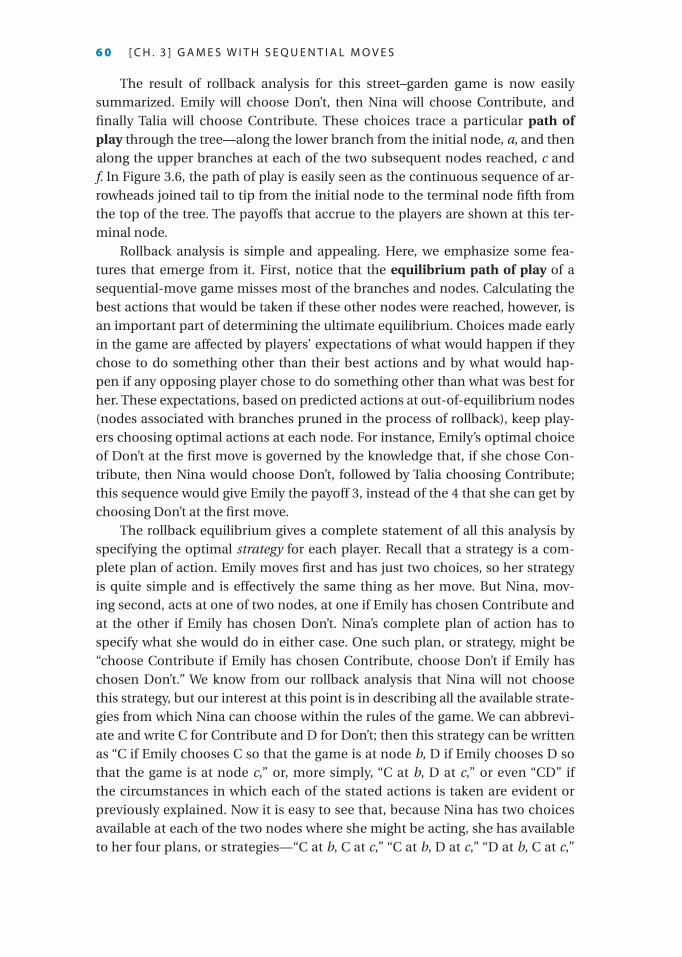
The result of rollback analysis for this street–garden game is now easily summarized. Emily will choose Don’t, then Nina will choose Contribute, and finally Talia will choose Contribute. These choices trace a particular path of play through the tree—along the lower branch from the initial node, a, and then along the upper branches at each of the two subsequent nodes reached, c and f. In Figure 3.6, the path of play is easily seen as the continuous sequence of ar-rowheads joined tail to tip from the initial node to the terminal node fifth from the top of the tree. The payoffs that accrue to the players are shown at this ter-minal node.

Rollback analysis is simple and appealing. Here, we emphasize some fea-tures that emerge from it. First, notice that the equilibrium path of play of a sequential-move game misses most of the branches and nodes. Calculating the best actions that would be taken if these other nodes were reached, however, is an important part of determining the ultimate equilibrium. Choices made early in the game are affected by players’ expectations of what would happen if they chose to do something other than their best actions and by what would hap-pen if any opposing player chose to do something other than what was best for her. These expectations, based on predicted actions at out-of-equilibrium nodes (nodes associated with branches pruned in the process of rollback), keep play-ers choosing optimal actions at each node. For instance, Emily’s optimal choice of Don’t at the first move is governed by the knowledge that, if she chose Con-tribute, then Nina would choose Don’t, followed by Talia choosing Contribute; this sequence would give Emily the payoff 3, instead of the 4 that she can get by choosing Don’t at the first move.

The rollback equilibrium gives a complete statement of all this analysis by specifying the optimal strategy for each player. Recall that a strategy is a com-plete plan of action. Emily moves first and has just two choices, so her strategy is quite simple and is effectively the same thing as her move. But Nina, mov-ing second, acts at one of two nodes, at one if Emily has chosen Contribute and at the other if Emily has chosen Don’t. Nina’s complete plan of action has to specify what she would do in either case. One such plan, or strategy, might be “choose Contribute if Emily has chosen Contribute, choose Don’t if Emily has chosen Don’t.” We know from our rollback analysis that Nina will not choose this strategy, but our interest at this point is in describing all the available strate-gies from which Nina can choose within the rules of the game. We can abbrevi-ate and write C for Contribute and D for Don’t; then this strategy can be written as “C if Emily chooses C so that the game is at node b, D if Emily chooses D so that the game is at node c,” or, more simply, “C at b, D at c,” or even “CD” if the circumstances in which each of the stated actions is taken are evident or previously explained. Now it is easy to see that, because Nina has two choices available at each of the two nodes where she might be acting, she has available to her four plans, or strategies—“C at b, C at c,” “C at b, D at c,” “D at b, C at c,”

6841D CH03 UG.indd 60 12/18/14 3:10 PM

and “D at b, D at c,” or “CC,” “CD,” “DC,” and “DD.” Of these strategies, the rollback analysis and the arrows at nodes b and c of Figure 3.6 show that her optimal strategy is “DC.”

Matters are even more complicated for Talia. When her turn comes, the his-tory of play can, according to the rules of the game, be any one of four possibilities. Talia’s turn to act comes at one of four nodes in the tree, one after Emily has chosen C and Nina has chosen C (node d), the second after Emily’s C and Nina’s D (node e), the third after Emily’s D and Nina’s C (node f ), and the fourth after both Emily and Nina choose D (node g). Each of Talia’s strategies, or complete plans of action, must specify one of her two actions for each of these four scenarios, or one of her two actions at each of her four possible action nodes. With four nodes at which to specify an action and with two actions from which to choose at each node, there are 2 2 2 2, or 16 possible combinations of actions. So Talia has available to her 16 possible strategies. One of them could be written as

“C at d, D at e, D at f, C at g” or “CDDC” for short,

where we have fixed the order of the four scenarios (the histories of moves by Emily and Nina) in the order of nodes d, e, f, and g. Then, with the use of the same abbreviation, the full list of 16 strategies available to Talia is

CCCC, CCCD, CCDC, CCDD, CDCC, CDCD, CDDC, CDDD, DCCC, DCCD, DCDC, DCDD, DDCC, DDCD, DDDC, DDDD.

Of these strategies, the rollback analysis of Figure 3.6 and the arrows at nodes d, e, f, and g show that Talia’s optimal strategy is DCCD.

Now we can express the findings of our rollback analysis by stating the strat-egy choices of each player—Emily chooses D from the two strategies available to her, Nina chooses DC from the four strategies available to her, and Talia chooses DCCD from the sixteen strategies available to her. When each player looks ahead in the tree to forecast the eventual outcomes of her current choices, she is cal-culating the optimal strategies of the other players. This configuration of strate-gies, D for Emily, DC for Nina, and DCCD for Talia, then constitutes the rollback equilibrium of the game.

We can put together the optimal strategies of the players to find the ac-tual path of play that will result in the rollback equilibrium. Emily will begin by choosing D. Nina, following her strategy DC, chooses the action C in response to Emily’s D. (Remember that Nina’s DC means “choose D if Emily has played C, and choose C if Emily has played D.”) According to the convention that we have adopted, Talia’s actual action after Emily’s D and then Nina’s C—from node f—is the third letter in the four-letter specification of her strategies. Because Talia’s optimal strategy is DCCD, her action along the path of play is C. Thus the actual path of play consists of Emily playing D, followed successively by Nina and Talia playing C.


6841D CH03 UG.indd 61 12/18/14 3:10 PM


To sum up, we have three distinct concepts:

1. The lists of available strategies for each player. The list, especially for later players, may be very long, because their actions in situations correspond-ing to all conceivable preceding moves by other players must be specified.

2. The optimal strategy, or complete plan of action for each player. This strategy must specify the player’s best choices at each node where the rules of the game specify that she moves, even though many of these nodes will never be reached in the actual path of play. This specification is in effect the preceding movers’ forecasting of what would happen if they took different actions and is therefore an important part of their cal-culation of their own best actions at the earlier nodes. The optimal strate-gies of all players together yield the rollback equilibrium.

3. The actual path of play in the rollback equilibrium, found by putting to-gether the optimal strategies for all the players.

4 ORDER ADVANTAGES

In the rollback equilibrium of the street–garden game, Emily gets her best out-come (payoff 4), because she can take advantage of the opportunity to make the first move. When she chooses not to contribute, she puts the onus on the other two players—each can get her next-best outcome if and only if both of them choose to contribute. Most casual thinkers about strategic games have the preconception that such a first-mover advantage should exist in all games. However, that is not the case. It is easy to think of games in which an oppor-tunity to move second is an advantage. Consider the strategic interaction be-tween two firms that sell similar merchandise from catalogs—say, Land’s End and L.L. Bean. If one firm had to release its catalog first, and then the second firm could see what prices the first had set before printing its own catalog, then the second mover could undercut its rival on all items and gain a tremendous competitive edge.

First-mover advantage comes from the ability to commit oneself to an ad-vantageous position and to force the other players to adapt to it; second-mover advantage comes from the flexibility to adapt oneself to the others’ choices. Whether commitment or flexibility is more important in a specific game de-pends on its particular configuration of strategies and payoffs; no generally valid rule can be laid down. We will come across examples of both kinds of advan-tages throughout this book. The general point that there need not be first-mover advantage, a point that runs against much common perception, is so important that we felt it necessary to emphasize at the outset.

6841D CH03 UG.indd 62 12/18/14 3:10 PM

When a game has a first- or second-mover advantage, each player may try to manipulate the order of play so as to secure for herself the advantageous posi-tion. Tactics for such manipulation are strategic moves, which we consider in Chapter 9.

5 ADDING MORE MOVES

We saw in Section 3 that adding more players increases the complexity of the analysis of sequential-play games. In this section, we consider another type of complexity that arises from adding additional moves to the game. We can do so most simply in a two-person game by allowing players to alternate moves more than once. Then the tree is enlarged in the same fashion as a multiple-player game tree would be, but later moves in the tree are made by the players who have made decisions earlier in the same game.

Many common games, such as tic-tac-toe, checkers, and chess, are two-person strategic games with such alternating sequential moves. The use of game trees and rollback should allow us to “solve” such games—to determine the rollback equilibrium outcome and the equilibrium strategies leading to that outcome. Unfortunately, as the complexity of the game grows and as strategies become more and more intricate, the search for an optimal solution becomes more and more difficult as well. In such cases, when manual solution is no longer really feasible, computer routines such as Gambit, mentioned in Chapter 2, become useful.

A. Tic-Tac-Toe

Start with the most simple of the three examples mentioned in the preceding paragraph, tic-tac-toe, and consider an easier-than-usual version in which two players (X and O) each try to be the first to get two of their symbols to fill any row, column, or diagonal of a two-by-two game board. The first player has four possible actions or positions in which to put her X. The second player then has three possible actions at each of four decision nodes. When the first player gets to her second turn, she has two possible actions at each of 12 (4 3) decision nodes. As Figure 3.7 shows, even this mini-game of tic-tac-toe has a very com-plex game tree. This tree is actually not too complex because the game is guar-anteed to end after the first player moves a second time, but there are still 24 terminal nodes to consider.

We show this tree merely as an illustration of how complex game trees can become in even simple (or simplified) games. As it turns out, using rollback on the mini-game of tic-tac-toe leads us quickly to an equilibrium. Rollback shows

a D D i n g m o r e m o v e s 6 3

6841D CH03 UG.indd 63 12/18/14 3:10 PM


that all of the choices for the first player at her second move lead to the same outcome. There is no optimal action; any move is as good as any other move. Thus, when the second player makes her first move, she also sees that each pos-sible move yields the same outcome, and she, too, is indifferent among her three choices at each of her four decision nodes. Finally, the same is true for the first player on her first move; any choice is as good as any other, so she is guaranteed to win the game.

Although this version of tic-tac-toe has an interesting tree, its solution is not as interesting. The first player always wins, so choices made by either player cannot affect the ultimate outcome. Most of us are more familiar with the three-by-three version of tic-tac-toe. To illustrate that version with a game tree, we would have to show that the first player has nine possible actions at the initial node, the second player has eight possible actions at each of nine decision nodes, and then the first player, on her second turn, has seven possible actions at each of 8 9 72 nodes, while the second player, on her second turn, has six possible actions at each of 7 8 9 504 nodes. This pattern continues until eventually the tree stops branching so rapidly because certain combina-tions of moves lead to a win for one player and the game ends. But no win is possible until at least the fifth move. Drawing the complete tree for this game requires a very large piece of paper or very tiny handwriting.

Most of you know, however, how to achieve at worst a tie when you play three-by-three tic-tac-toe. So there is a simple solution to this game that can be

X wins

X wins

X wins

X wins

X wins

X wins

X wins

X wins

X wins

X wins

X wins

X wins

X wins X wins X wins X wins X wins X wins

X wins X wins X wins X wins X wins X wins

Player X

Player X

Player X

Player X

Player X

Player X

Player XPlayer XPlayer XPlayer X

Player XPlayer XPlayer X

Player X

Bottomright

Bottomleft

Bottomright

Bottomleft

Bottomright

Bottomright

Bottomright

Bottomleft

Bottomright

Bottomleft

Bottomleft

Bottomleft

Topright

Topright

Topright

Topright

Topright

Topleft

Topleft

Topleft

Topleft

Topleft

Topleft

Player O Player O

Player O

Bottom

left

Bottom

left

Bottomright

Player O

Bottomright

Bottomleft

Bottomright

Bottomright

Bottomleft

Topright

Topright

Topright

Top

right

Top

right

Topleft

Topleft

Topleft

Topleft

Figure 3.7 the Complex tree for simple two-by-two tic-tac-toe

6841D CH03 UG.indd 64 12/18/14 3:10 PM

found by rollback, and a learned strategic thinker can reduce the complexity of the game considerably in the quest for such a solution. It turns out that, as in the two-by-two version, many of the possible paths through the game tree are stra-tegically identical. Of the nine possible initial moves, there are only three types; you put your X in either a corner position (of which there are four possibilities), a side position (of which there are also four possibilities), or the (one) middle position. Using this method to simplify the tree can help reduce the complexity of the problem and lead you to a description of an optimal rollback equilibrium strategy. Specifically, we could show that the player who moves second can al-ways guarantee at least a tie with an appropriate first move and then by con-tinually blocking the first player’s attempts to get three symbols in a row.3

B. Chess

Although relatively small games, such as tic-tac-toe, can be solved using rollback, we showed above how rapidly the complexity of game trees can increase even in two-player games. Thus when we consider more complicated games, such as chess, finding a complete solution becomes much more difficult.

In chess, the players, White and Black, have a collection of 16 pieces in six distinct shapes, each of which is bound by specified rules of movement on the eight-by-eight game board shown in Figure 3.8.4 White opens with a move, Black responds with one, and so on, in turns. All the moves are visible to the other player, and nothing is left to chance, as it would be in card games that include shuffling and dealing. Moreover, a chess game must end in a finite number of moves. The rules declare that a game is drawn if a given position on the board is repeated three times in the course of play. Because there are a finite number of ways to place the 32 (or fewer after captures) pieces on 64 squares, a game could not go on infinitely long without running up against this rule. Therefore, in principle, chess is amenable to full rollback analysis.

That rollback analysis has not been carried out, however. Chess has not been “solved” as tic-tac-toe has been. And the reason is that, for all its simplicity of rules, chess is a bewilderingly complex game. From the initial set position of


3 If the first player puts her first symbol in the middle position, the second player must put her first symbol in a corner position. Then the second player can guarantee a tie by taking the third position in any row, column, or diagonal that the first player tries to fill. If the first player goes to a corner or a side position first, the second player can guarantee a tie by going to the middle first and then fol-lowing the same blocking technique. Note that if the first player picks a corner, the second player picks the middle, and the first player then picks the corner opposite from her original play, then the second player must not pick one of the remaining corners if she is to ensure at least a tie. For a beau-tifully detailed picture of the complete contigent strategy in tic-tac-toe, see the online comic strip at http://xkcd.com/832/.4 An easily accessible statement of the rules of chess and much more is at Wikipedia, at http://en.wikipedia.org/wiki/Chess.

6841D CH03 UG.indd 65 12/18/14 3:10 PM


the pieces illustrated in Figure 3.8, White can open with any one of 20 moves,5 and Black can respond with any of 20. Therefore, 20 branches emerge from the first node of the game tree, each leading to a second node from each of which 20 more branches emerge. After only two moves, there are already 400 branches, each leading to a node from which many more branches emerge. And the total number of possible moves in chess has been estimated to be 10120, or a “one” with 120 zeros after it. A supercomputer a thousand times as fast as your PC, making a trillion calculations a second, would need more than 10100 years to check out all these moves.6 Astronomers offer us less than 1010 years before the sun turns into a red giant and swallows the earth.

The general point is that, although a game may be amenable in principle to a complete solution by rollback, its complete tree may be too complex to permit such solution in practice. Faced with such a situation, what is a player to do? We can learn a lot about this by reviewing the history of attempts to program com-puters to play chess.

When computers first started to prove their usefulness for complex calcula-tions in science and business, many mathematicians and computer scientists

5 He can move one of eight pawns forward either one square or two or he can move one of the two knights in one of two ways (to squares a3, c3, f3, or h3).6 This would have to be done only once because, after the game has been solved, anyone can use the solution and no one will actually need to play. Everyone will know whether White has a win or whether Black can force a draw. Players will toss to decide who gets which color. They will then know the outcome, shake hands, and go home.

♛ ♚ ♞♞ ♜♜ ♝♝

d e gb ha

8

7

6

5

4

3

2

1

8

7

6

5

4

3

2

1

fc

d e gb ha fc

♕ ♔ ♘♘ ♖♖ ♗♗

♟ ♟ ♟♟ ♟♟ ♟♟

♙ ♙ ♙♙ ♙♙ ♙♙

Figure 3.8 Chessboard

6841D CH03 UG.indd 66 12/18/14 3:10 PM

thought that a chess-playing computer program would soon beat the world champion. It took a lot longer, even though computer technology improved dra-matically while human thought progressed much more slowly. Finally, in De-cember 1992, a German chess program called Fritz2 beat world champion Gary Kasparov in some blitz (high-speed) games. Under regular rules, where each player gets 2¹-2 hours to make 40 moves, humans retained greater superiority for longer. A team sponsored by IBM put a lot of effort and resources into the devel-opment of a specialized chess-playing computer and its associated software. In February 1996, this package, called Deep Blue, was pitted against Gary Kasparov in a best-of-six series. Deep Blue caused a sensation by winning the first game, but Kasparov quickly figured out its weaknesses, improved his counterstrate-gies, and won the series handily. In the next 15 months, the IBM team improved Deep Blue’s hardware and software, and the resulting Deeper Blue beat Kasparov in another best-of-six series in May 1997.

To sum up, computers have progressed in a combination of slow patches and some rapid spurts, while humans have held some superiority but have not been able to improve sufficiently fast to keep ahead. Closer examination reveals that the two use quite different approaches to think through the very complex game tree of chess.

When contemplating a move in chess, looking ahead to the end of the whole game may be too hard (for humans and computers both). How about looking part of the way—say, 5 or 10 moves ahead—and working back from there? The game need not end within this limited horizon; that is, the nodes that you reach after 5 or 10 moves will not generally be terminal nodes. Only terminal nodes have payoffs specified by the rules of the game. Therefore, you need some indi-rect way of assigning plausible payoffs to nonterminal nodes, because you are not able to explicitly roll back from a full look-ahead. A rule that assigns such payoffs is called an intermediate valuation function.

In chess, humans and computer programs both use such partial look-ahead in conjunction with an intermediate valuation function. The typical method as-signs values to each piece and to positional and combinational advantages that can arise during play. Quantification of values for different positions are made on the basis of the whole chess-playing community’s experience of play in past games starting from such positions or patterns; this is called “knowledge.” The sum of all the numerical values attached to pieces and their combinations in a position is the intermediate value of that position. A move is judged by the value of the position to which it is expected to lead after an explicit forward-looking calculation for a cer-tain number—say, five or six—of moves.

The evaluation of intermediate positions has progressed furthest with re-spect to chess openings—that is, the first dozen or so moves of a game. Each opening can lead to any one of a vast multitude of further moves and positions, but experience enables players to sum up certain openings as being more or less


6841D CH03 UG.indd 67 12/18/14 3:10 PM


likely to favor one player or the other. This knowledge has been written down in massive books of openings, and all top players and computer programs remem-ber and use this information.

At the end stages of a game, when only a few pieces are left on the board, backward reasoning on its own is often simple enough to be doable and com-plete enough to give the full answer. The midgame, when positions have evolved into a level of complexity that will not simplify within a few moves, is the hardest to analyze. To find a good move from a midgame position, a well-built interme-diate valuation function is likely to be more valuable than the ability to calculate another few moves further ahead.

This is where the art of chess playing comes into its own. The best human players develop an intuition or instinct that enables them to sniff out good op-portunities and avoid subtle traps in a way that computer programs find hard to match. Computer scientists have found it generally very difficult to teach their machines the skills of pattern recognition that humans acquire and use instinctively—for example, recognizing faces and associating them with names. The art of the midgame in chess also is an exercise in recognizing and evaluat-ing patterns in the same, still mysterious way. This is where Kasparov has his greatest advantage over Fritz2 or Deep Blue. It also explains why computer pro-grams do better against humans at blitz or limited-time games: a human does not have the time to marshal his art of the midgame.

In other words, the best human players have subtle “chess knowledge,” based on experience or the ability to recognize patterns, which endows them with a better intermediate valuation function. Computers have the advantage when it comes to raw or brute-force calculation. Thus although both human and computer players now use a mixture of look-ahead and intermediate valuation, they use them in different proportions: humans do not look so many moves ahead but have better intermediate valuations based on knowledge; computers have less sophisticated valuation functions but look ahead further by using their superior computational powers.

Recently, chess computers have begun to acquire more knowledge. When modifying Deep Blue in 1996 and 1997, IBM enlisted the help of human experts to improve the intermediate valuation function in its software. These consul-tants played repeatedly against the machine, noted its weaknesses, and sug-gested how the valuation function should be modified to correct the flaws. Deep Blue benefited from the contributions of the experts and their subtle kind of thinking, which results from long experience and an awareness of complex interconnections among the pieces on the board.

If humans can gradually make explicit their subtle knowledge and trans-mit it to computers, what hope is there for human players who do not get re-ciprocal help from computers? At times in their 1997 encounter, Kasparov was amazed by the human or even superhuman quality of Deep Blue’s play. He even

6841D CH03 UG.indd 68 12/18/14 3:10 PM

attributed one of the computer’s moves to “the hand of God.” And matters can only get worse: the brute-force calculating power of computers is increasing rapidly while they are simultaneously, but more slowly, gaining some of the sub-tlety that constitutes the advantage of humans.

The abstract theory of chess says that it is a finite game that can be solved by rollback. The practice of chess requires a lot of “art” based on experi-ence, intuition, and subtle judgment. Is this bad news for the use of rollback in sequential-move games? We think not. It is true that theory does not take us all the way to an answer for chess. But it does take us a long way. Looking ahead a few moves constitutes an important part of the approach that mixes brute-force calculation of moves with a knowledge-based assessment of intermediate po-sitions. And, as computational power increases, the role played by brute-force calculation, and therefore the scope of the rollback theory, will also increase.

Evidence from the study of the game of checkers, as we describe below, sug-gests that a solution to chess may yet be feasible.

C. Checkers

An astonishing number of computer and person hours have been devoted to the search for a solution to chess. Less famously, but just as doggedly, researchers worked on solving the somewhat less complex game of checkers. And, indeed, the game of checkers was declared “solved” in July 2007.7

Checkers is another two-player game played on an eight-by-eight board. Each player has 12 round game pieces of different colors, as shown in Figure 3.9, and players take turns moving their pieces diagonally on the board, jump-ing (and capturing) the opponent’s pieces when possible. As in chess, the game ends and Player A wins when Player B is either out of pieces or unable to move; the game can also end in a draw if both players agree that neither can win.

Although the complexity of checkers pales somewhat in comparison to that of chess—the number of possible positions in checkers is approximately the square root of the number in chess—there are still 5 1020 possible positions, so drawing a game tree is out of the question. Conventional wisdom and evidence from world championships for years suggested that good play should lead to a draw, but there was no proof. Now a computer scientist in Canada has the proof—a computer program named Chinook that can play to a guaranteed tie.

Chinook was first created in 1989. This computer program played the world champion, Marion Tinsley, in 1992 (losing four to two with 33 draws) and again in 1994 (when Tinsley’s health failed during a series of draws). It was put on


7 Our account is based on two reports in the journal Science. See Adrian Cho, “Program Proves That Checkers, Perfectly Played, Is a No-Win Situation,” Science, vol. 317 (July 20, 2007), pp. 308–309, and Jonathan Schaeffer et al., “Checkers Is Solved,” Science, vol. 317 (September 14, 2007), pp. 1518–22.

6841D CH03 UG.indd 69 12/18/14 3:10 PM


hold between 1997 and 2001 while its creators waited for computer technol-ogy to improve. And it finally exhibited a loss-proof algorithm in the spring of 2007. That algorithm uses a combination of endgame rollback analysis and starting position forward analysis along with the equivalent of an intermediate valuation function to trace out the best moves within a database including all possible positions on the board.

The creators of Chinook describe the full game of checkers as “weakly solved”; they know that they can generate a tie, and they have a strategy for reaching that tie from the start of the game. For all 39 1012 possible positions that include 10 or fewer pieces on the board, they describe checkers as “strongly solved”; not only do they know they can play to a tie, they can reach that tie from any of the possible positions that can arise once only 10 pieces remain. Their al-gorithm first solved the 10-piece endgames, then went back to the start to search out paths of play in which both players make optimal choices. The search mech-anism, involving a complex system of evaluating the value of each intermediate position, invariably led to those 10-piece positions that generate a draw.

Thus, our hope for the future of rollback analysis may not be misplaced. We know that for really simple games, we can find the rollback equilibrium by verbal reasoning without having to draw the game tree explicitly. For games having an intermediate range of complexity, verbal reasoning is too hard, but a complete tree can be drawn and used for rollback. Sometimes we may enlist the aid of a computer to draw and analyze a moderately complicated game tree. For the most complex games, such as checkers and chess, we can

Figure 3.9 Checkers

6841D CH03 UG.indd 70 12/18/14 3:10 PM

draw only a small part of the game tree, and we must use a combination of two methods: (1) calculation based on the logic of rollback, and (2) rules of thumb for valuing intermediate positions on the basis of experience. The computa-tional power of current algorithms has shown that even some games in this category are amenable to solution, provided one has the time and resources to devote to the problem.

Thankfully, most of the strategic games that we encounter in economics, politics, sports, business, and daily life are far less complex than chess or even checkers. The games may have a number of players who move a number of times; they may even have a large number of players or a large number of moves. But we have a chance at being able to draw a reasonable-looking tree for those games that are sequential in nature. The logic of rollback remains valid, and it is also often the case that, once you understand the idea of rollback, you can carry out the necessary logical thinking and solve the game without explicitly drawing a tree. Moreover, it is precisely at this intermediate level of difficulty, between the simple examples that we solved explicitly in this chapter and the insoluble cases such as chess, that computer software such as Gambit is most likely to be useful; this is indeed fortunate for the prospect of applying the theory to solve many games in practice.

6 EVIDENCE CONCERNING ROLLBACK

How well do actual participants in sequential-move games perform the cal-culations of rollback reasoning? There is very little systematic evidence, but class-room and research experiments with some games have yielded outcomes that appear to counter the predictions of the theory. Some of these experiments and their outcomes have interesting implications for the strategic analysis of sequential-move games.

For instance, many experimenters have had subjects play a single-round bargaining game in which two players, designated A and B, are chosen from a class or a group of volunteers. The experimenter provides a dollar (or some known total), which can be divided between them according to the following procedure: Player A proposes a split—for example, “75 to me, 25 to B.” If player B accepts this proposal, the dollar is divided as proposed by A. If B rejects the proposal, neither player gets anything.

Rollback in this case predicts that B should accept any sum, no matter how small, because the alternative is even worse—namely, 0—and, foreseeing this, A should propose “99 to me, 1 to B.” This particular outcome almost never happens. Most players assigned the A role propose a much more equal split. In fact, 50–50 is the single most common proposal. Furthermore, most players assigned the B

e v i D e n C e C o n C e r n i n g r o l l b a C k 7 1

6841D CH03 UG.indd 71 12/18/14 3:10 PM


role turn down proposals that leave them 25% or less of the total and walk away with nothing; some reject proposals that would give them 40% of the pie.8

Many game theorists remain unpersuaded that these findings undermine the theory. They counter with some variant of the following argument: “The sums are so small as to make the whole thing trivial in the players’ minds. The B players lose 25 or 40 cents, which is almost nothing, and perhaps gain some pri-vate satisfaction that they walked away from a humiliatingly small award. If the total were a thousand dollars, so that 25% of it amounted to real money, the B players would accept.” But this argument does not seem to be valid. Experiments with much larger stakes show similar results. The findings from experiments con-ducted in Indonesia, with sums that were small in dollars but amounted to as much as three months’ earnings for the participants, showed no clear tendency on the part of the A players to make less equal offers, although the B players tended to accept somewhat smaller shares as the total increased; similar experi-ments conducted in the Slovak Republic found the behavior of inexperienced players unaffected by large changes in payoffs.9

The participants in these experiments typically have no prior knowledge of game theory and no special computational abilities. But the game is extremely simple; surely even the most naive player can see through the reasoning, and answers to direct questions after the experiment generally show that most par-ticipants do. The results show not so much the failure of rollback as the theorist’s error in supposing that each player cares only about her own money earnings. Most societies instill in their members a strong sense of fairness, which causes the B players to reject anything that is grossly unfair. Anticipating this, the A players offer relatively equal splits.

Supporting evidence comes from the new field of “neuroeconomics.” Alan Sanfey and his colleagues took MRI readings of the players’ brains as they made their choices in the ultimatum game. They found stimulation of “activity in a region well known for its involvement in negative emotion” in the brains of responders (B players) when they rejected “unfair” (less than 50;50) offers. Thus, deep instincts or emotions of anger and disgust seem to be implicated in these rejections. They also found that “unfair” (less than 50;50) offers were

8 Reiley first encountered this game as a graduate student; he was stunned that when he offered a 90:10 split of $100, the other economics graduate student rejected it. For a detailed account of this game and related ones, read Richard H. Thaler, “Anomalies: The Ultimate Game,” Journal of Eco-nomic Perspectives, vol. 2, no. 4 (Fall 1988), pp. 195–206; and Douglas D. Davis and Charles A. Holt, Experimental Economics (Princeton: Princeton University Press, 1993), pp. 263–69.9 The results of the Indonesian experiment are reported in Lisa Cameron, “Raising the Stakes in the Ultimatum Game: Experimental Evidence from Indonesia,” Economic Inquiry, vol. 37, no. 1 (Janu-ary 1999), pp. 47–59. Robert Slonim and Alvin Roth report results similar to Cameron’s, but they also found that offers (in all rounds of play) were rejected less often as the payoffs were raised. See Robert Slonim and Alvin Roth, “Learning in High Stakes Ultimatum Games: An Experiment in the Slovak Republic,” Econometrica, vol. 66, no. 3 (May 1998), pp. 569–96.

6841D CH03 UG.indd 72 12/18/14 3:10 PM

rejected less often when responders knew that the offerer was a computer than when they knew that the offerer was human.10

Notably, A players have some tendency to be generous even without the threat of retaliation. In a drastic variant called the dictator game, where the A player decides on the split and the B player has no choice at all, many As still give significant shares to the Bs, suggesting the players have some intrinsic preference for relatively equal splits.11 However, the offers by the A players are noticeably less generous in the dictator game than in the ultimatum game, sug-gesting that the credible fear of retaliation is also a strong motivator. Caring about other people’s perceptions of us also appears to matter. When the experi-mental design is changed so that not even the experimenter can identify who proposed (or accepted) the split, the extent of sharing drops noticeably.

Another experimental game with similarly paradoxical outcomes goes as follows: two players are chosen and designated as A and B. The experimenter puts a dime on the table. Player A can take it or pass. If A takes the dime, the game is over, with A getting the 10 cents and B getting nothing. If A passes, the experimenter adds a dime, and now B has the choice of taking the 20 cents or passing. The turns alternate, and the pile of money grows until reaching some limit—say, a dollar—that is known in advance by both players.

We show the tree for this game in Figure 3.10. Because of the appearance of the tree, this type of game is often called the centipede game. You may not even need the tree to use rollback on this game. Player B is sure to take the dollar at the last stage, so A should take the 90 cents at the penultimate stage, and so on. Thus, A should take the very first dime and end the game.

In experiments, however, such games typically go on for at least a few rounds. Remarkably, by behaving “irrationally,” the players as a group make

e v i D e n C e C o n C e r n i n g r o l l b a C k 7 3

10 See Alan Sanfey, James Rilling, Jessica Aronson, Leigh Nystrom, and Jonathan Cohen, “The Neural Basis of Economic Decision-Making in the Ultimatum Game,” Science, vol. 300 (June 13, 2003), pp. 1755–58.11 One could argue that this social norm of fairness may actually have value in the ongoing evolu-tionary game being played by the whole society. Players who are concerned with fairness reduce transaction costs and the costs of fights, which can be beneficial to society in the long run. These matters will be discussed in Chapters 10 and 11.

Takedimes

Takedimes

Takedimes

Takedimes

Takedime

Pass Pass Pass Pass PassA B A B B

10, 0 0, 20 30, 0 0, 40 0, 100

0, 0

Figure 3.10 the Centipede game

6841D CH03 UG.indd 73 12/18/14 3:10 PM


more money than they would if they followed the logic of backward reasoning. Sometimes A does better and sometimes B, but sometimes they even solve this conflict or bargaining problem. In a classroom experiment that one of us (Dixit) conducted, one such game went all the way to the end. Player B collected the dollar, and quite voluntarily gave 50 cents to player A. Dixit asked A, “Did you two conspire? Is B a friend of yours?” and A replied, “No, we didn’t even know each other before. But he is a friend now.” We will come across some similar evi-dence of cooperation that seems to contradict rollback reasoning when we look at finitely repeated prisoners’ dilemma games in Chapter 10.

The centipede game points out a possible problem with the logic of roll-back in non-zero-sum games, even for players whose decisions are only based on money. Note that if Player A passes in the first round, he has already shown himself not to be playing rollback. So what should Player B expect him to do in round 3? Having passed once, he might pass again, which would make it rational for Player B to pass in round 2. Eventually someone will take the pile of money, but an initial deviation from rollback equilibrium makes it difficult to predict exactly when this will happen. And because the size of the pie keeps growing, if I see you deviate from rollback, I might want to deviate as well, at least for a little while. A player might deliberately pass in an early round in order to signal a willingness to pass in future rounds. This problem does not arise in zero-sum games, where there is no incentive to cooperate by waiting.

Supporting this observation, Steven Levitt, John List, and Sally Sadoff con-ducted experiments with world-class chess players, finding more rollback behavior in zero-sum sequential-move games than in the non-zero-sum centi-pede game. Their centipede game involved six nodes, with total payoffs increas-ing quite steeply across rounds.12 While there are considerable gains to players who can manage to pass back and forth to each other, the rollback equilibrium specifies playing Take at each node. In stark contrast to the theory, only 4% of players played Take at node 1, providing little support for rollback equilibrium even in this simple six-move game. (The fraction of players who played Take in-creased over the course of the game.13)

12 See Steven D. Levitt, John A. List, and Sally E. Sadoff, “Checkmate: Exploring Backward Induction Among Chess Players,” American Economic Review, vol. 101, no. 2 (April 2011), pp. 975–90. The de-tails of the game tree are as follows. If A plays Take at node 1, then A receives $4 while B receives $1. If A passes and B plays Take at node 2, then A receives $2 while B receives $8. This pattern of doubling continues until node 6, where if B plays Take, the payoffs are $32 for A and $128 for B, but if B plays Pass, the payoffs are $256 for A and $64 for B.13 Different results were found in an earlier paper by Ignacio Palacios-Huerta and Oscar Volij, “Field Centipedes,” American Economic Review, vol. 99, no. 4 (September 2009), pp. 1619–35. Of the chess players they studied, 69% played Take at the first node, with the more highly rated chess players being more likely to play Take at the first opportunity. These results indicated a surprisingly high ability of players to carry experience with them to a new game context, but these results have not been reproduced in the later paper discussed above.

6841D CH03 UG.indd 74 12/18/14 3:10 PM

By contrast, in a zero-sum sequential-move game whose rollback equilib-rium involves 20 moves (you are invited to solve such a game in Exercise S7), the chess players played the exact rollback equilibrium 10 times as often as in the six-move centipede game.14

Levitt and his coauthors also experimented with a similar but more diffi-cult zero-sum game (a version of which you are invited to solve in Exercise U5). There the chess players played the complete rollback equilibrium only 10% of the time (20% for the highest-ranked grandmasters), although by the last few moves the agreement with rollback was nearly 100%. As world-class chess play-ers spend tens of thousands of hours trying to win chess games by rolling back, these results indicate that even highly experienced players usually cannot im-mediately carry their experience over to a new game: they need a little expe-rience with the new game before they can figure out the optimal strategy. An advantage of learning game theory is that you can more easily spot underlying similarities between seemingly different situations and so devise good strategies more quickly in any new games you may face.

The examples discussed here seem to indicate that apparent violations of strategic logic can often be explained by recognizing that people do not care merely about their own money payoffs; rather, they internalize concepts such as fairness. But not all observed plays, contrary to the precepts of rollback, have such an explanation. People do fail to look ahead far enough, and they do fail to draw the appropriate conclusions from attempts to look ahead. For example, when issuers of credit cards offer favorable initial interest rates or no fees for the first year, many people fall for them without realizing that they may have to pay much more later. Therefore the game-theoretic analysis of rollback and rollback equilibria serves an advisory or prescriptive role as much as it does a descrip-tive role. People equipped with the theory of rollback are in a position to make better strategic decisions and to get higher payoffs, no matter what they include in their payoff calculations. And game theorists can use their expertise to give valuable advice to those who are placed in complex strategic situations but lack the skill to determine their own best strategies.

7 STRATEGIES IN SURVIVOR

The examples in the preceding sections were deliberately constructed to illustrate and elucidate basic concepts such as nodes, branches, moves, and strategies,

s t r at e g i e s i n s u r v i v o r 7 5

14 As you will see in the exercises, another key distinction of this zero-sum game is that there is a way for one player to guarantee victory, regardless of what the other player does. By contrast, a play-er’s best move in the centipede game depends on what she expects the other player to do.

6841D CH03 UG.indd 75 12/18/14 3:10 PM


as well as the technique of rollback. Now we show how all of them can be ap-plied, by considering a real-life (or at least “reality-TV-life”) situation.

In the summer of 2000, CBS television broadcast the first of the Survivor shows, which became an instant hit and helped launch the whole new genre of “reality TV.” Leaving aside many complex details and some earlier stages not relevant for our purpose, the concept was as follows: a group of contestants, called a “tribe,” was put on an uninhabited island and left largely to fend for themselves for food and shelter. Every three days, they had to vote one fellow contestant out of the tribe. The person who had the most votes cast against him or her at a meeting of the remaining players (called the “tribal council”) was the victim of the day. However, before each meeting of the tribal council, the survivors up to that point competed in a game of physical or mental skill that was devised by the producers of the game for that occasion, and the winner of this competition, called a “challenge,” was immune from being voted off at the following meeting. Also, one could not vote against oneself. Finally, when two people were left, the seven who had been voted off most recently returned as a “jury” to pick one of the two remaining survivors as the million-dollar winner of the whole game.

The strategic problems facing all contestants were: (1) to be generally re-garded as a productive contributor to the tribe’s search for food and other tasks of survival, but to do so without being regarded as too strong a competitor and therefore a target for elimination; (2) to form alliances to secure blocks of votes to protect oneself from being voted off; (3) to betray these alliances when the numbers got too small and one had to vote against someone; but (4) to do so without seriously losing popularity with the other players, who would ultimately have the power of the vote on the jury.

We pick up the story when just three contestants were left: Rudy, Kelly, and Rich. Of them, Rudy was the oldest contestant, an honest and blunt person who was very popular with the contestants who had been previously voted off. It was generally agreed that, if he was one of the last two, then he would be voted the million-dollar winner. So it was in the interests of both Kelly and Rich that they should face each other, rather than face Rudy, in the final vote. But neither wanted to be seen as instrumental in voting off Rudy. With just three contestants left, the winner of the immunity challenge is effectively decisive in the cast-off vote, because the other two must vote against each other. Thus, the jury would know who was responsible for voting off Rudy and, given his popularity, would regard the act of voting him off with disfavor. The person doing so would harm his or her chances in the final vote. This was especially a problem for Rich, be-cause he was known to have an alliance with Rudy.

The immunity challenge was one of stamina: each contestant had to stand on an awkward support and lean to hold one hand in contact with a totem on a

6841D CH03 UG.indd 76 12/18/14 3:10 PM

central pole, called the “immunity idol.” Anyone whose hand lost contact with the idol, even for an instant, lost the challenge; the one to hold on longest was the winner.

An hour and a half into the challenge, Rich figured out that his best strategy was to deliberately lose this immunity challenge. Then, if Rudy won immunity, he would maintain his alliance and keep Rich—Rudy was known to be a man who always kept his word. Rich would lose the final vote to Rudy in this case, but that would make him no worse off than if he won the challenge and kept Rudy. If Kelly won immunity, the much more likely outcome, then it would be in her interest to vote off Rudy—she would have at least some chance against Rich but none against Rudy. Then Rich’s chances of winning were quite good. Whereas, if Rich himself held on, won immunity, and then voted off Rudy, his chances against Kelly would be decreased by the fact that he voted off Rudy.

So Rich deliberately stepped off and later explained his reasons quite clearly to the camera. His calculation was borne out. Kelly won that challenge and voted off Rudy. And, in the final jury vote between Rich and Kelly, Rich won by one vote.

Rich’s thinking was essentially a rollback analysis along a game tree. He did this analysis instinctively, without drawing the tree, while standing awkwardly and holding on to the immunity idol, but it took him an hour and a half to come to his conclusion. With all due credit to Rich, we show the tree explicitly, and can reach the answer faster.

Figure 3.11 shows the tree. You can see that it is much more complex than the trees encountered in earlier sections. It has more branches and moves; in addition, there are uncertain outcomes, and the chances of winning or losing in various alternative situations have to be estimated instead of being known pre-cisely. But you will see how we can make reasonable assumptions about these chances and proceed with the analysis.

At the initial node, Rich decides whether to continue or to give up in the im-munity challenge. In either case, the winner of the challenge cannot be forecast with certainty; this is indicated in the tree by letting “Nature” make the choice, as we did with the coin-toss situation in Figure 3.1. If Rich continues, Nature chooses the winner from the three contestants. We don’t know the actual prob-abilities, but we will assume particular values for exposition and point out the crucial assumptions. The supposition is that Kelly has a lot of stamina and that Rudy, being the oldest, is not likely to win. So we posit the following probabilities of a win when Rich chooses to continue: 0.5 (50%) for Kelly, 0.45 for Rich, and only 0.05 for Rudy. If Rich gives up on the challenge, Nature picks the winner of the immunity challenge randomly between the two who remain; in this case, we assume that Kelly wins with probability 0.9 and Rudy with probability 0.1.

The rest of the tree follows from each of the three possible winners of the challenge. If Rudy wins, he keeps Rich as he promised, and the jury votes Rudy


6841D CH03 UG.indd 77 12/18/14 3:10 PM


the winner.15 If Rich wins immunity, he has to decide whether to keep Kelly or Rudy. If he keeps Rudy, the jury votes for Rudy. If he keeps Kelly, it is not certain whom the jury chooses. We assume that Rich alienates some jurors by turning on Rudy and that, despite being better liked than Kelly, he gets the jury’s vote in this situation only with probability 0.4. Similarly, if Kelly wins immunity, she can either keep Rudy and lose the jury’s vote, or keep Rich. If she keeps Rich, his

JURY PICKS

Rich 0.4

Rich keeps

Kellykeeps

Rudy keeps

Rudy keeps

Kellykeeps

Rudy Rudy

Rich wins Prob. = 0.18

Kelly wins

Rudy wins

Kelly0.6

Kelly

Naturepicks

immunitywinner

Naturepicks

immunitywinner

Rich prob. 0.45

Rudy prob. 0.05

Kellyprob. 0.9

Rudy prob. 0.1

Kellyprob. 0.5

JURY PICKS

JURY PICKS

Rich wins with prob. = 0.18 + 0.3 = 0.48

Rich wins with prob. = 0.54

Rich 0.6

Rudy Rudy


Kelly wins

Rudy wins

Kelly0.4

Rich

Continue

Give up

JURY PICKS

JURY PICKS

Rich 0.6

Rudy Rudy


Kelly wins

Rudy wins

Kelly0.4

Rich

Rich

JURY PICKS

Rudy Rudy wins JURY

PICKS

Rudy

Rich

Rich Rudy wins JURY

PICKS

Figure 3.11 survivor immunity game tree

15 Technically, Rudy faces a choice between keeping Rich or Kelly at the action node after he wins the immunity challenge. Because everyone placed 0 probability on his choosing Kelly (owing to the Rich-Rudy alliance), we illustrate only Rudy’s choice of Rich. The jury, similarly, has a choice be-tween Rich and Rudy at the last action node along this branch of play. Again, the foregone conclu-sion is that Rudy wins in this case.

6841D CH03 UG.indd 78 12/18/14 3:10 PM

probability of winning the jury’s vote is higher, at 0.6, because in this case he is both better liked by the jury and hasn’t voted off Rudy.

What about the players’ actual payoffs? We can safely assume that both Rich and Kelly want to maximize the probability of his or her emerging as the ulti-mate winner of the $1 million. Rudy similarly wants to get the prize, but keeping his word to Rich is paramount. With these preferences of the various players in mind, Rich can now do rollback analysis along the tree to determine his own initial choice.

Rich knows that, if he wins the immunity challenge (the uppermost path after his own first move and Nature’s move), he will have to keep Kelly to have a 40% chance of eventual victory; keeping Rudy at this stage would mean a 0 probability of eventual victory. Rich can also calculate that, if Kelly wins the im-munity challenge (which occurs once in each of the upper and lower halves of the tree), she will choose to keep him for similar reasons, and then the probabil-ity of his eventual victory will be 0.6.

What are Rich’s chances as he calculates them at the initial node? If Rich chooses Give Up at the initial node, then there is only one way for him to emerge as the eventual winner—if Kelly wins immunity (probability 0.9), if she then keeps Rich (probability 1), and if the jury votes for Rich (probability 0.6). Because all three things need to happen for Rich to win, his overall prob-ability of victory is the product of the three probabilities—namely, 0.9 1 0.6 0.54.16 If Rich chooses Continue at the initial node, then there are two ways in which he can win. First, he wins the game if he wins the immunity challenge (probability 0.45), if he then eliminates Rudy (probability 1), and if he still wins the jury’s vote against Kelly (probability 0.4); the total probability of winning in this way is 0.45 0.4 0.18. Second, he wins the game if Kelly wins the chal-lenge (probability 0.5), if she eliminates Rudy (probability 1), and if Rich gets the jury’s vote (probability 0.6); total probability here is 0.5 0.6 0.3. Rich’s overall probability of eventual victory if he chooses Continue is the sum of the prob-abilities of these two paths to victory—namely, 0.18 0.3 0.48.

Rich can now compare his probability of winning the million dollars when he chooses Give Up (0.54) with his probability of winning when he chooses Con-tinue (0.48). Given the assumed values of the various probabilities in the tree, Rich has a better chance of victory if he gives up. Thus, Give Up is his optimal strategy. Although this result is based on assuming specific numbers for the probabilities, Give Up remains Rich’s optimal strategy as long as (1) Kelly is very likely to win the immunity challenge once Rich gives up, and (2) Rich wins the jury’s final vote more often when Kelly has voted out Rudy than when Rich has done so.17


16 Readers who need instruction or a refresher course in the rules for combining probabilities will find a quick tutorial in the appendix to Chapter 7.17 Readers who can handle the algebra of probabilities can solve this game by using more general symbols instead of specific numbers for the probabilities, as in Exercise U10 of this chapter.

6841D CH03 UG.indd 79 12/18/14 3:10 PM


This example serves several purposes. Most important, it shows how a complex tree, with much external uncertainty and missing information about precise probabilities, can still be solved by using rollback analysis. We hope this gives you some confidence in using the method and some training in converting a somewhat loose verbal account into a more precise logical ar-gument. You might counter that Rich did this reasoning without drawing any trees. But knowing the system or general framework greatly simplifies the task even in new and unfamiliar circumstances. Therefore it is definitely worth the effort to acquire the systematic skill.

A second purpose is to illustrate the seemingly paradoxical strategy of “los-ing to win.” Another instance of this strategy can be found in some sporting competitions that are held in two rounds, such as the soccer World Cup. The first round is played on a league basis in several groups of four teams each. The top two teams from each group then go to the second round, where they play others chosen according to a prespecified pattern; for example, the top-ranked team in group A meets the second-ranked team in group B, and so on. In such a situ-ation, it may be good strategy for a team to lose one of its first-round matches if this loss causes it to be ranked second in its group; that ranking might earn it a subsequent match against a team that, for some particular reason, it is more likely to beat than the team that it would meet if it had placed first in its group in the first round.

SUMMARY

Sequential-move games require players to consider the future conse-quences of their current moves before choosing their actions. Analysis of pure sequential-move games generally requires the creation of a game tree. The tree is made up of nodes and branches that show all of the possible actions available to each player at each of her opportunities to move, as well as the payoffs as-sociated with all possible outcomes of the game. Strategies for each player are complete plans that describe actions at each of the player’s decision nodes con-tingent on all possible combinations of actions made by players who acted at earlier nodes. The equilibrium concept employed in sequential-move games is that of rollback equilibrium, in which players’ equilibrium strategies are found by looking ahead to subsequent nodes and the actions that would be taken there and by using these forecasts to calculate one’s current best action. This process is known as rollback, or backward induction.

Different types of games entail advantages for different players, such as first-mover advantages. The inclusion of many players or many moves enlarges the game tree of a sequential-move game but does not change the solution

6841D CH03 UG.indd 80 12/18/14 3:10 PM

process. In some cases, drawing the full tree for a particular game may re-quire more space or time than is feasible. Such games can often be solved by identifying strategic similarities between actions that reduce the size of the tree or by simple logical thinking.

When solving larger games, verbal reasoning can lead to the rollback equi-librium if the game is simple enough or a complete tree may be drawn and ana-lyzed. If the game is sufficiently complex that verbal reasoning is too difficult and a complete tree is too large to draw, we may enlist the help of a computer program. Checkers has been “solved” with the use of such a program, although full solution of chess will remain beyond the powers of computers for a long time. In actual play of these truly complex games, elements of both art (identifi-cation of patterns and of opportunities versus peril) and science (forward-looking calculations of the possible outcomes arising from certain moves) have a role in determining player moves.

Tests of the theory of sequential-move games seem to suggest that actual play shows the irrationality of the players or the failure of the theory to predict behavior adequately. The counterargument points out the complexity of actual preferences for different possible outcomes and the usefulness of strategic the-ory for identifying optimal actions when actual preferences are known.

KEY TERMS

action node (48) intermediate valuation function (67) backward induction (56) move (50) branch (48) node (48) decision node (48) path of play (60) decision tree (48) prune (54) equilibrium path of play (60) rollback (56) extensive form (48) rollback equilibrium (56) first-mover advantage (62) root (48) game tree (48) second-mover advantage (62) initial node (48) terminal node (50)

SOLVED ExERCISES

S1. Suppose two players, Hansel and Gretel, take part in a sequential-move game. Hansel moves first, Gretel moves second, and each player moves only once.

(a) Draw a game tree for a game in which Hansel has two possible ac-tions (Up or Down) at each node and Gretel has three possible

e x e r C i s e s 8 1

6841D CH03 UG.indd 81 12/18/14 3:10 PM


actions (Top, Middle, or Bottom) at each node. How many of each node type—decision and terminal—are there?

(b) Draw a game tree for a game in which Hansel and Gretel each have three possible actions (Sit, Stand, or Jump) at each node. How many of the two node types are there?

(c) Draw a game tree for a game in which Hansel has four possible ac-tions (North, South, East, or West) at each node and Gretel has two possible actions (Stay or Go) at each node. How many of the two node types are there?

S2. In each of the following games, how many pure strategies (complete plans of action) are available to each player? List out all of the pure strat-egies for each player.

(a)

N

SCARECROW

S

tTINMAN

b 2, 1

1, 0

0, 2

SCARECROW

(b)

n

TINMAN s

N SCARECROW

S

n

TINMAN s

N SCARECROW

S

n

TINMAN s

N

S

0, 1

5, 4

2, 3

3, 2 2, 2

1, 0

4, 5

(c)

tTINMAN

b

N

SCARECROW S

u

LION d

N

S SCARECROW

0, 2, 0

0, 0, 2

2, 3, 2

1, 1, 1

3, 3, 3

1, 2, 4

N

S

SCARECROW

6841D CH03 UG.indd 82 12/18/14 3:10 PM

S3. For each of the games illustrated in Exercise S2, identify the rollback equi-librium outcome and the complete equilibrium strategy for each player.

S4. Consider the rivalry between Airbus and Boeing to develop a new com-mercial jet aircraft. Suppose Boeing is ahead in the development process and Airbus is considering whether to enter the competition. If Airbus stays out, it earns 0 profit, whereas Boeing enjoys a monopoly and earns a profit of $1 billion. If Airbus decides to enter and develop the rival airplane, then Boeing has to decide whether to accommodate Airbus peaceably or to wage a price war. In the event of peaceful competition, each firm will make a profit of $300 million. If there is a price war, each will lose $100 million because the prices of airplanes will fall so low that neither firm will be able to recoup its development costs.

Draw the tree for this game. Find the rollback equilibrium and de-scribe the firms’ equilibrium strategies.

S5. Consider a game in which two players, Fred and Barney, take turns re-moving matchsticks from a pile. They start with 21 matchsticks, and Fred goes first. On each turn, each player may remove either one, two, three, or four matchsticks. The player to remove the last matchstick wins the game.

(a) Suppose there are only six matchsticks left, and it is Barney’s turn. What move should Barney make to guarantee himself victory? Ex-plain your reasoning.

(b) Suppose there are 12 matchsticks left, and it is Barney’s turn. What move should Barney make to guarantee himself victory? (Hint: Use your answer to part (a) and roll back.)

(c) Now start from the beginning of the game. If both players play opti-mally, who will win?

(d) What are the optimal strategies (complete plans of action) for each player?

S6. Consider the game in the previous exercise. Suppose the players have reached a point where it is Fred’s move and there are just five matchsticks left.

(a) Draw the game tree for the game starting with five matchsticks. (b) Find the rollback equilibria for this game starting with five

matchsticks. (c) Would you say this five-matchstick game has a first-mover advan-

tage or a second-mover advantage? (d) Explain why you found more than one rollback equilibrium. How is

your answer related to the optimal strategies you found in part (c) of the previous exercise?


6841D CH03 UG.indd 83 12/18/14 3:10 PM


S7. Elroy and Judy play a game that Elroy calls the “race to 100.” Elroy goes first, and the players take turns choosing numbers between one and nine. On each turn, they add the new number to a running total. The player who brings the total exactly to 100 wins the game.

(a) If both players play optimally, who will win the game? Does this game have a first-mover advantage? Explain your reasoning.

(b) What are the optimal strategies (complete plans of action) for each player?

S8. A slave has just been thrown to the lions in the Roman Colosseum. Three lions are chained down in a line, with Lion 1 closest to the slave. Each lion’s chain is short enough that he can only reach the two players imme-diately adjacent to him.

The game proceeds as follows. First, Lion 1 decides whether or not to eat the slave.

If Lion 1 has eaten the slave, then Lion 2 decides whether or not to eat Lion 1 (who is then too heavy to defend himself). If Lion 1 has not eaten the slave, then Lion 2 has no choice: he cannot try to eat Lion 1, because a fight would kill both lions.

Similarly, if Lion 2 has eaten Lion 1, then Lion 3 decides whether or not to eat Lion 2.

Each lion’s preferences are fairly natural: best (4) is to eat and stay alive, next best (3) is to stay alive but go hungry, next (2) is to eat and be eaten, and worst (1) is to go hungry and be eaten.

(a) Draw the game tree, with payoffs, for this three-player game. (b) What is the rollback equilibrium to this game? Make sure to de-

scribe the strategies, not just the payoffs. (c) Is there a first-mover advantage to this game? Explain why or why

not. (d) How many complete strategies does each lion have? List them.

S9. Consider three major department stores—Big Giant, Titan, and Frieda’s—contemplating opening a branch in one of two new Boston-area shop-ping malls. Urban Mall is located close to the large and rich population center of the area; it is relatively small and can accommodate at most two department stores as “anchors” for the mall. Rural Mall is farther out in a rural and relatively poorer area; it can accommodate as many as three anchor stores. None of the three stores wants to have branches in both malls because there is sufficient overlap of customers between the malls that locating in both would just mean competing with itself. Each store prefers to be in a mall with one or more other department stores than to be alone in the same mall, because a mall with multiple department

6841D CH03 UG.indd 84 12/18/14 3:10 PM

stores will attract sufficiently many more total customers that each store’s profit will be higher. Further, each store prefers Urban Mall to Rural Mall because of the richer customer base. Each store must choose between trying to get a space in Urban Mall (knowing that if the attempt fails, it will try for a space in Rural Mall) and trying to get a space in Rural Mall right away (without even attempting to get into Urban Mall).

In this case, the stores rank the five possible outcomes as follows: 5 (best), in Urban Mall with one other department store; 4, in Rural Mall with one or two other department stores; 3, alone in Urban Mall; 2, alone in Rural Mall; and 1 (worst), alone in Rural Mall after having attempted to get into Urban Mall and failed, by which time other nondepartment stores have signed up the best anchor locations in Rural Mall.

The three stores are sufficiently different in their managerial struc-tures that they experience different lags in doing the paperwork required to request an expansion space in a new mall. Frieda’s moves quickly, followed by Big Giant, and finally by Titan, which is the least efficient in readying a location plan. When all three have made their requests, the malls decide which stores to let in. Because of the name recognition that both Big Giant and Titan have with the potential customers, a mall would take either (or both) of those stores before it took Frieda’s. Thus, Frieda’s does not get one of the two spaces in Urban Mall if all three stores re-quest those spaces; this is true even though Frieda’s moves first.

(a) Draw the game tree for this mall location game. (b) Illustrate the rollback pruning process on your game tree and use

the pruned tree to find the rollback equilibrium. Describe the equi-librium by using the (complete) strategies employed by each de-partment store. What are the payoffs to each store at the rollback equilibrium outcome?

S10. (Optional ) Consider the following ultimatum bargaining game, which has been studied in laboratory experiments. The Proposer moves first, and proposes a split of $10 between himself and the Responder. Any whole-dollar split may be proposed. For example, the Proposer may offer to keep the whole $10 for himself, he may propose to keep $9 for himself and give $1 to the Responder, $8 to himself and $2 to the Responder, and so on. (Note that the Proposer therefore has eleven possible choices.) After seeing the split, the Responder can choose to accept the split or re-ject it. If the Responder accepts, both players get the proposed amounts. If she rejects, both players get $0.

(a) Write out the game tree for this game. (b) How many complete strategies does each player have?


6841D CH03 UG.indd 85 12/18/14 3:10 PM

(c) What is the rollback equilibrium to this game, assuming the players care only about their cash payoffs?

(d) Suppose Rachel the Responder would accept any offer of $3 or more, and reject any offer of $2 or less. Suppose Pete the Proposer knows Rachel’s strategy, and he wants to maximize his cash payoff. What strategy should he use?

(e) Rachel’s true payoff (her “utility”) might not be the same as her cash payoff. What other aspects of the game might she care about? Given your answer, propose a set of payoffs for Rachel that would make her strategy optimal.

(f) In laboratory experiments, players typically do not play the rollback equilibrium. Proposers typically offer an amount between $2 and $5 to the Responder. Responders often reject offers of $3, $2, and espe-cially $1. Explain why you think this might occur.

UNSOLVED ExERCISES

U1. “In a sequential-move game, the player who moves first is sure to win.” Is this statement true or false? State the reason for your answer in a few brief sentences, and give an example of a game that illustrates your answer.

U2. In each of the following games, how many pure strategies (complete plans of action) are available to each player? List all of the pure strategies for each player.


(a)

N

EALBUS

S

a

MINERVA

b5, 0

1, 1

a

MINERVA

b 2, 1

3, 0

a

MINERVAb

1, 5

4, 4

N

ALBUS

ALBUS

S

NMINERVA

S1, 3

5, 2a

bc 0, 4

3, 3

a

MINERVAb 3, 1

2, 2

(b)

N

ALBUS

S

X

SEVERUS

MINERVA MINERVA

ALBUS

Y

N

S 2, 4, 0

1, 3, 1

a

b4, 1, 5

0, 2, 3a

b0, 4, 4

2, 1, 1

(c)

6841D CH03 UG.indd 86 12/18/14 3:10 PM

U3. For each of the games illustrated in Exercise U2, identify the rollback equilibrium outcome and the complete equilibrium strategy for each player.

U4. Two distinct proposals, A and B, are being debated in Washington. Con-gress likes proposal A, and the president likes proposal B. The proposals are not mutually exclusive; either or both or neither may become law. Thus there are four possible outcomes, and the rankings of the two sides are as follows, where a larger number represents a more favored outcome:


Outcome Congress President

A becomes law 4 1

B becomes law 1 4

Both A and B become law 3 3

Neither (status quo prevails) 2 2

(a)

N

EALBUS

S

a

MINERVA

b5, 0

1, 1

a

MINERVA

b 2, 1

3, 0

a

MINERVAb

1, 5

4, 4

N

ALBUS

ALBUS

S

NMINERVA

S1, 3

5, 2a

bc 0, 4

3, 3

a

MINERVAb 3, 1

2, 2

(b)

N

ALBUS

S

X

SEVERUS

MINERVA MINERVA

ALBUS

Y

N

S 2, 4, 0

1, 3, 1

a

b4, 1, 5

0, 2, 3a

b0, 4, 4

2, 1, 1

(c)

6841D CH03 UG.indd 87 12/18/14 3:10 PM

(a) The moves in the game are as follows. First, Congress decides whether to pass a bill and whether the bill is to contain A or B or both. Then the president decides whether to sign or veto the bill. Congress does not have enough votes to override a veto. Draw a tree for this game and find the rollback equilibrium.

(b) Now suppose the rules of the game are changed in only one respect: the president is given the extra power of a line-item veto. Thus, if Congress passes a bill containing both A and B, the president may choose not only to sign or veto the bill as a whole, but also to veto just one of the two items. Show the new tree and find the rollback equilibrium.

(c) Explain intuitively why the difference between the two equilibria arises.

U5. Two players, Amy and Beth, play the following game with a jar contain-ing 100 pennies. The players take turns; Amy goes first. Each time it is a player’s turn, she takes between 1 and 10 pennies out of the jar. The player whose move empties the jar wins.

(a) If both players play optimally, who will win the game? Does this game have a first-mover advantage? Explain your reasoning.

(b) What are the optimal strategies (complete plans of action) for each player?

U6. Consider a slight variant to the game in Exercise U5. Now the player whose move empties the jar loses.

(a) Does this game have a first-mover advantage? (b) What are the optimal strategies for each player?

U7. Kermit and Fozzie play a game with two jars, each containing 100 pen-nies. The players take turns; Kermit goes first. Each time it is a player’s turn, he chooses one of the jars and removes anywhere from 1 to 10 pen-nies from it. The player whose move leaves both jars empty wins. (Note that when a player empties the second jar, the first jar must already have been emptied in some previous move by one of the players.)

(a) Does this game have a first-mover advantage or a second-mover ad-vantage? Explain which player can guarantee victory, and how he can do it. (Hint: Simplify the game by starting with a smaller number of pennies in each jar, and see if you can generalize your finding to the actual game.)

(b) What are the optimal strategies (complete plans of action) for each player? (Hint: First think of a starting situation in which both jars have equal numbers of pennies. Then consider starting positions in which the two jars differ by 1 to 10 pennies. Finally, consider starting positions in which the jars differ by more than 10 pennies.)


6841D CH03 UG.indd 88 12/18/14 3:10 PM


U8. Modify Exercise S8 so that there are now four lions. (a) Draw the game tree, with payoffs, for this four-player game. (b) What is the rollback equilibrium to this game? Make sure to de-

scribe the strategies, not just the payoffs. (c) Is the additional lion good or bad for the slave? Explain.

U9. To give Mom a day of rest, Dad plans to take his two children, Bart and Cassie, on an outing on Sunday. Bart prefers to go to the amusement park (A), whereas Cassie prefers to go to the science museum (S). Each child gets 3 units of utility from his/her more preferred activity and only 2 units of utility from his/her less preferred activity. Dad gets 2 units of utility for either of the two activities.

To choose their activity, Dad plans first to ask Bart for his preference, then to ask Cassie after she hears Bart’s choice. Each child can choose ei-ther the amusement park (A) or the science museum (S). If both children choose the same activity, then that is what they will all do. If the children choose different activities, Dad will make a tie-breaking decision. As the parent, Dad has an additional option: he can choose the amusement park, the science museum, or his personal favorite, the mountain hike (M). Bart and Cassie each get 1 unit of utility from the mountain hike, and Dad gets 3 units of utility from the mountain hike.

Because Dad wants his children to cooperate with one another, he gets 2 extra units of utility if the children choose the same activity (no matter which one of the two it is).

(a) Draw the game tree, with payoffs, for this three-person game. (b) What is the rollback equilibrium to this game? Make sure to de-

scribe the strategies, not just the payoffs. (c) How many different complete strategies does Bart have? Explain. (d) How many complete strategies does Cassie have? Explain.

U10. (Optional—more difficult) Consider the Survivor game tree illustrated in Figure 3.11. We might not have guessed exactly the values Rich estimated for the various probabilities, so let’s generalize this tree by considering other possible values. In particular, suppose that the probability of win-ning the immunity challenge when Rich chooses Continue is x for Rich, y for Kelly, and 1 x y for Rudy; similarly, the probability of winning when Rich gives up is z for Kelly and 1 z for Rudy. Further, suppose that Rich’s chance of being picked by the jury is p if he has won immu-nity and has voted Rudy off the island; his chance of being picked is q if Kelly has won immunity and has voted Rudy off the island. Continue to assume that if Rudy wins immunity, he keeps Rich with probability 1, and that Rudy wins the game with probability 1 if he ends up in the final two. Note that in the example of Figure 3.11, we had x 0.45, y 0.5,

6841D CH03 UG.indd 89 12/18/14 3:10 PM


z 0.9, p 0.4, and q 0.6. (In general, the variables p and q need not sum to 1, though this happened to be true in Figure 3.11.)

(a) Find an algebraic formula, in terms of x, y, z, p, and q, for the prob-ability that Rich wins the million dollars if he chooses Continue. (Note: Your formula might not contain all of these variables.)

(b) Find a similar algebraic formula for the probability that Rich wins the million dollars if he chooses Give Up. (Again, your formula might not contain all of the variables.)

(c) Use these results to find an algebraic inequality telling us under what circumstances Rich should choose Give Up.

(d) Suppose all the values are the same as in Figure 3.11 except for z. How high or low could z be so that Rich would still prefer to Give Up? Explain intuitively why there are some values of z for which Rich is better off choosing Continue.

(e) Suppose all the values are the same as in Figure 3.11 except for p and q. Assume that since the jury is more likely to choose a “nice” person who doesn’t vote Rudy off, we should have p . 0.5 . q. For what values of the ratio (p q)should Rich choose Give Up? Explain intuitively why there are some values of p and q for which Rich is better off choosing Continue.

6841D CH03 UG.indd 90 12/18/14 3:10 PM

games with sequential moves - obviously awesome

Documents