game theory with engineering applications 15: repeated games - ocw.mit.edu · game theory: lecture...

6.254 : Game Theory with Engineering ApplicationsLecture 15: Repeated Games

Asu OzdaglarMIT

April 1, 2010

1

Game Theory: Lecture 15 Introduction

Outline

Repeated Games (perfect monitoring) The problem of cooperation Finitely-repeated prisoner’s dilemma Infinitely-repeated games and cooperation

Folk Theorems

Reference:

Fudenberg and Tirole, Section 5.1.

2


Prisoners’ Dilemma

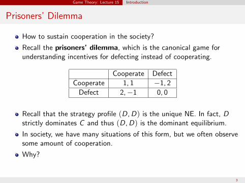
How to sustain cooperation in the society?

Recall the prisoners’ dilemma, which is the canonical game for understanding incentives for defecting instead of cooperating.

Cooperate Defect Cooperate 1, 1 −1, 2

Defect 2, −1 0, 0

Recall that the strategy profile (D, D) is the unique NE. In fact, D strictly dominates C and thus (D, D) is the dominant equilibrium.

In society, we have many situations of this form, but we often observe some amount of cooperation.

Why?

3


Repeated Games

In many strategic situations, players interact repeatedly over time.

Perhaps repetition of the same game might foster cooperation.

By repeated games, we refer to a situation in which the same stage game (strategic form game) is played at each date for some duration of T periods.

Such games are also sometimes called “supergames”.

We will assume that overall payoff is the sum of discounted payoffs at each stage.

Future payoffs are discounted and are thus less valuable (e.g., money and the future is less valuable than money now because of positive interest rates; consumption in the future is less valuable than consumption now because of time preference).

We will see in this lecture how repeated play of the same strategic game introduces new (desirable) equilibria by allowing players to condition their actions on the way their opponents played in the previous periods.

4


Discounting

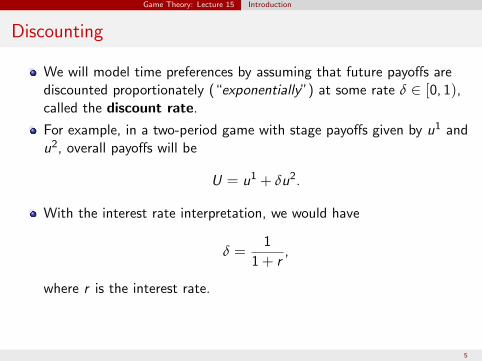
We will model time preferences by assuming that future payoffs are discounted proportionately (“exponentially”) at some rate δ ∈ [0, 1), called the discount rate.

For example, in a two-period game with stage payoffs given by u1 and u2, overall payoffs will be

U = u 1 + δu 2 .

With the interest rate interpretation, we would have

1 δ = ,

1 + r

where r is the interest rate.

5

� �


Mathematical Model

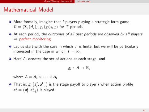
More formally, imagine that I players playing a strategic form game G = �I , (Ai )i ∈I , (gi )i∈I � for T periods.

At each period, the outcomes of all past periods are observed by all players ⇒ perfect monitoring

Let us start with the case in which T is finite, but we will be particularly interested in the case in which T = ∞.

Here Ai denotes the set of actions at each stage, and

gi : A R,→

where A = A1 × · · · × AI .

That is, gi ait , at is the stage payoff to player i when action profile � � −i

at = ait , at is played.−i

6


Mathematical Model (continued)

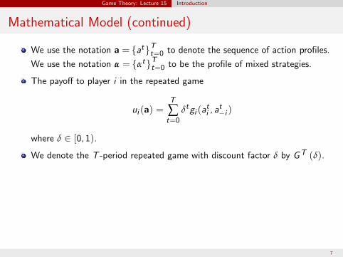
We use the notation a = {at } T

T =0 to denote the sequence of action profiles. t

We use the notation α = {αt }t=0 to be the profile of mixed strategies.

The payoff to player i in the repeated game

T ui (a) = ∑ δt gi (ai

t , a t )−i t=0

where δ ∈ [0, 1).

We denote the T -period repeated game with discount factor δ by G T (δ).

7


Finitely-Repeated Prisoners’ Dilemma

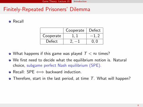
Recall


Defect 2, −1 0, 0

What happens if this game was played T < ∞ times?

We first need to decide what the equilibrium notion is. Natural choice, subgame perfect Nash equilibrium (SPE).

Recall: SPE backward induction. ⇐⇒

Therefore, start in the last period, at time T . What will happen?

8


Finitely-Repeated Prisoners’ Dilemma (continued)

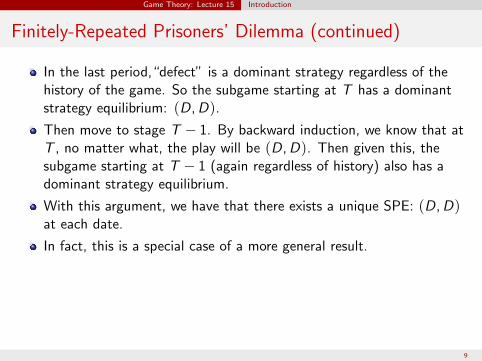
In the last period,“defect” is a dominant strategy regardless of the history of the game. So the subgame starting at T has a dominant strategy equilibrium: (D, D). Then move to stage T − 1. By backward induction, we know that atT , no matter what, the play will be (D, D). Then given this, thesubgame starting at T − 1 (again regardless of history) also has adominant strategy equilibrium.

With this argument, we have that there exists a unique SPE: (D, D)at each date.

In fact, this is a special case of a more general result.

9


Equilibria of Finitely-Repeated Games

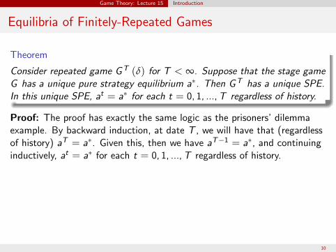
Theorem

Consider repeated game G T (δ) for T < ∞. Suppose that the stage game G has a unique pure strategy equilibrium a∗. Then G T has a unique SPE. In this unique SPE, at = a∗ for each t = 0, 1, ..., T regardless of history.

Proof: The proof has exactly the same logic as the prisoners’ dilemma example. By backward induction, at date T , we will have that (regardless of history) aT = a∗. Given this, then we have aT −1 = a∗, and continuing inductively, at = a∗ for each t = 0, 1, ..., T regardless of history.

10

Game Theory: Lecture 15 Infinitely-Repeated Games

Infinitely-Repeated Games

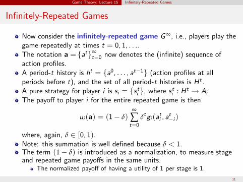
Now consider the infinitely-repeated game G ∞, i.e., players play the game repeatedly at times t The notation a = {at

action profiles.

∞ t=0}

= 0, 1, . . ..now denotes the (infinite) sequence of

A period-t history is ht = {a0 , . . . , at−1} (action profiles at all periods before t), and the set of all period-t histories is Ht . A pure strategy for player i is si = {sit }, where si

t : Ht Ai→The payoff to player i for the entire repeated game is then

ui (a) = (1 − δ) ∞

∑ t=0

δt gi (ait , a−

ti )

where, again, δ ∈ [0, 1).Note: this summation is well defined because δ < 1.The term (1 − δ) is introduced as a normalization, to measure stageand repeated game payoffs in the same units.

The normalized payoff of having a utility of 1 per stage is 1.

11

�


Trigger Strategies

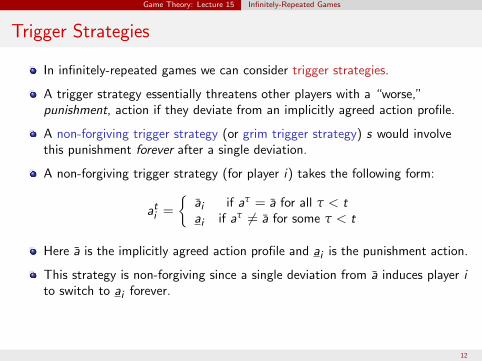
In infinitely-repeated games we can consider trigger strategies.

A trigger strategy essentially threatens other players with a “worse,” punishment, action if they deviate from an implicitly agreed action profile.

A non-forgiving trigger strategy (or grim trigger strategy) s would involve this punishment forever after a single deviation.

A non-forgiving trigger strategy (for player i) takes the following form:

a for all τ < t¯i if aτ =ai �

ai if aτ =a t =

Here a is the implicitly agreed action profile and ai

This strategy is non-forgiving since a single deviation from

¯ is the punishment action.

a induces player i to switch to ai forever.

¯ for some τ < ta

12


Cooperation with Trigger Strategies in the Repeated Prisoners’ Dilemma

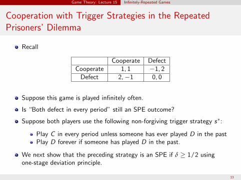
Recall


Defect 2, −1 0, 0

Suppose this game is played infinitely often.

Is “Both defect in every period” still an SPE outcome?

Suppose both players use the following non-forgiving trigger strategy s∗:

Play C in every period unless someone has ever played D in the past Play D forever if someone has played D in the past.

We next show that the preceding strategy is an SPE if δ ≥ 1/2 using one-stage deviation principle.

13


Cooperation with Trigger Strategies in the Repeated Prisoners’ Dilemma

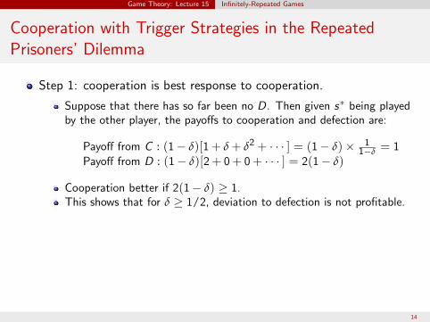
Step 1: cooperation is best response to cooperation.

Suppose that there has so far been no D. Then given s∗ being played by the other player, the payoffs to cooperation and defection are:

Payoff from C : (1 − δ)[1 + δ + δ2 + ] = (1 − δ) × 1 = 1 Payoff from D : (1 − δ)[2 + 0 + 0 +

· · · ] = 2(1 − δ)

1−δ · · ·

Cooperation better if 2(1 − δ) ≥ 1. This shows that for δ ≥ 1/2, deviation to defection is not profitable.

14


Cooperation with Trigger Strategies in the Repeated Prisoners’ Dilemma (continued)

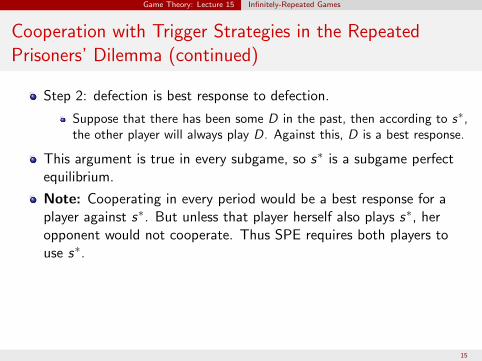
Step 2: defection is best response to defection.

Suppose that there has been some D in the past, then according to s∗, the other player will always play D. Against this, D is a best response.

This argument is true in every subgame, so s∗ is a subgame perfect equilibrium.

Note: Cooperating in every period would be a best response for a player against s∗. But unless that player herself also plays s∗, her opponent would not cooperate. Thus SPE requires both players to use s∗.

15


Remarks

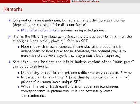
Cooperation is an equilibrium, but so are many other strategy profiles(depending on the size of the discount factor)

Multiplicity of equilibria endemic in repeated games.

If a∗ is the NE of the stage game (i.e., it is a static equilibrium), then the strategies “each player, plays ai

∗” form an SPE.

Note that with these strategies, future play of the opponent is independent of how I play today, therefore, the optimal play is to maximize the current payoff, i.e., play a static best response.)

Sets of equilibria for finite and infinite horizon versions of the “same game” can be quite different.

Multiplicity of equilibria in prisoner’s dilemma only occurs at T = ∞. In particular, for any finite T (and thus by implication for T ∞),→prisoners’ dilemma has a unique SPE. Why? The set of Nash equilibria is an upper semicontinuous correspondence in parameters. It is not necessarily lower semicontinuous.

16


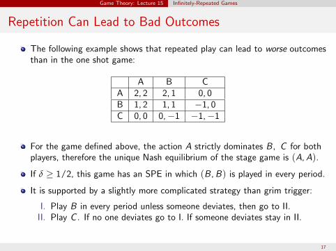
Repetition Can Lead to Bad Outcomes

The following example shows that repeated play can lead to worse outcomes than in the one shot game:

A B C A 2, 2 2, 1 0, 0 B 1, 2 1, 1 −1, 0 C 0, 0 0, −1 −1, −1

For the game defined above, the action A strictly dominates B, C for both players, therefore the unique Nash equilibrium of the stage game is (A, A).

If δ ≥ 1/2, this game has an SPE in which (B, B) is played in every period.

It is supported by a slightly more complicated strategy than grim trigger:

I. Play B in every period unless someone deviates, then go to II. II. Play C . If no one deviates go to I. If someone deviates stay in II.

17

Game Theory: Lecture 15 Folk Theorems

Folk Theorems

In fact, it has long been a “folk theorem” that one can support cooperation in repeated prisoners’ dilemma, and other “non-one-stage“equilibrium outcomes in infinitely-repeated games with sufficiently high discount factors.

These results are referred to as “folk theorems” since they were believed to be true before they were formally proved.

Here we will see a relatively strong version of these folk theorems.

18


Feasible Payoffs

Consider stage game G = �I , (Ai )i∈I , (gi )i∈I � and infinitely-repeatedgame G ∞ (δ).Let us introduce the set of feasible payoffs:

V = Conv{v ∈ RI | there exists a ∈ A such that g (a) = v }.

That is, V is the convex hull of all I - dimensional vectors that can be obtained by some action profile. Convexity here is obtained by public randomization.

Note: V is not equal to {v ∈ RI | there exists α ∈ Σ such that g (α) = v }, where Σ is the set of mixed strategy profiles in the stage game.

19

� �


Minmax Payoffs

Minmax payoff of player i : the lowest payoff that player i ’s opponent can hold him to:

v i = min max gi (αi , α−i ) . α−i αi

The player can never receive less than this amount.

Minmax strategy profile against i : � �

m i −i = arg minα−i

max αi

gi (αi , α−i )

iFinally, let m denote the strategy of player i such thati gi (mi

i , m−i

i ) = v i .

20


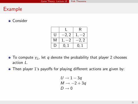
Example

Consider

L R U −2, 2 1, −2 M 1, −2 −2, 2 D 0, 1 0, 1

To compute v1, let q denote the probability that player 2 chooses action L.

Then player 1’s payoffs for playing different actions are given by:

U 1 − 3q→M → −2 + 3q D 0→

21


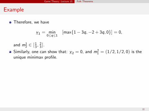
Example

Therefore, we have

v1 = min [max{1 − 3q, −2 + 3q, 0}] = 0,0≤q≤1

and m21 ∈ [ 13 ,

2 ].3

Similarly, one can show that: v2 = 0, and m12 = (1/2, 1/2, 0) is the

unique minimax profile.

22

1

2


Minmax Payoff Lower Bounds

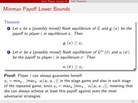
Theorem

Let α be a (possibly mixed) Nash equilibrium of G and gi (α) be the payoff to player i in equilibrium α. Then

gi (α) ≥ v i .

Let σ be a (possibly mixed) Nash equilibrium of G ∞ (δ) and ui (σ) be the payoff to player i in equilibrium σ. Then

ui (σ) ≥ v i .

Proof: Player i can always guarantee herself v i = mina [maxai ui (ai , a−i )] in the stage game and also in each stage −i

of the repeated game, since v i = maxai [mina ui (ai , a−i )], meaning that −i

she can always achieve at least this payoff against even the most adversarial strategies.

23

1

2


Folk Theorems

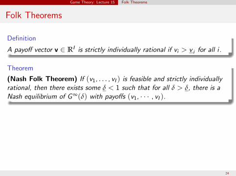
Definition

A payoff vector v ∈ RI is strictly individually rational if vi > v i for all i .

Theorem

(Nash Folk Theorem) If (v1, . . . , vI ) is feasible and strictly individually rational, then there exists some δ < 1 such that for all δ > δ, there is a Nash equilibrium of G ∞(δ) with payoffs (v1, · · · , vI ).

24


Proof

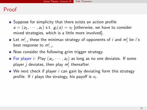
Suppose for simplicity that there exists an action profile a = (a1, [otherwise, we have to consider · · · , aI ) s.t. gi (a) = vi

mixed strategies, which is a little more involved].

Let mi these the minimax strategy of opponents of i and mi be i ’s−i i best response to mi

−i .

Now consider the following grim trigger strategy.

For player i : Play (a1, · · · , aI ) as long as no one deviates. If some player j deviates, then play mi

j thereafter.

We next check if player i can gain by deviating form this strategy profile. If i plays the strategy, his payoff is vi .

25

� �

� �


Proof (continued)

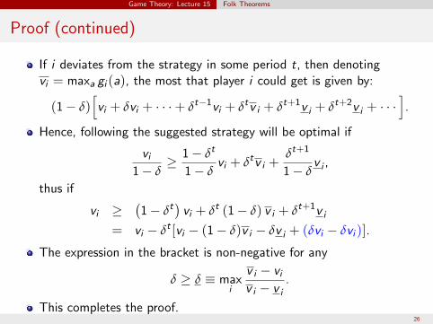
If i deviates from the strategy in some period t, then denoting vi = maxa gi (a), the most that player i could get is given by:

(1 − δ) vi + δvi + + δt−1 vi + δt v i + δt+1 v i + δt+2 v i + .· · · · · ·

Hence, following the suggested strategy will be optimal if

vi 1 − δt δt+1

1 − δ ≥

1 − δ vi + δt v i +

1 − δ v i ,

thus if

vi ≥ 1 − δt vi + δt (1 − δ) v i + δt+1 v i

= vi − δt [vi − (1 − δ)v i − δv i + (δvi − δvi )].

The expression in the bracket is non-negative for any

δ ≥ δ ≡ max v i − vi

. i v i − v i

This completes the proof. 26


Problems with Nash Folk Theorem

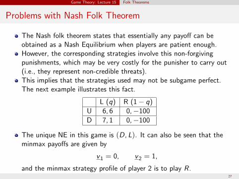
The Nash folk theorem states that essentially any payoff can be obtained as a Nash Equilibrium when players are patient enough. However, the corresponding strategies involve this non-forgiving punishments, which may be very costly for the punisher to carry out (i.e., they represent non-credible threats). This implies that the strategies used may not be subgame perfect. The next example illustrates this fact.

L (q) R (1 − q) U 6, 6 0, −100 D 7, 1 0, −100

The unique NE in this game is (D, L). It can also be seen that the minmax payoffs are given by

v1 = 0, v2 = 1,

and the minmax strategy profile of player 2 is to play R. 27


Problems with the Nash Folk Theorem (continued)

Nash Folk Theorem says that (6,6) is possible as a Nash equilibrium payoff of the repeated game, but the strategies suggested in the proof require player 2 to play R in every period following a deviation.

While this will hurt player 1, it will hurt player 2 a lot, it seems unreasonable to expect her to carry out the threat.

Our next step is to get the payoff (6, 6) in the above example, or more generally, the set of feasible and strictly individually rational payoffs as subgame perfect equilibria payoffs of the repeated game.

28

MIT OpenCourseWarehttp://ocw.mit.edu

6.254 Game Theory with Engineering Applications Spring 2010

For information about citing these materials or our Terms of Use, visit: http://ocw.mit.edu/terms.

http://ocw.mit.edu

http://ocw.mit.edu/terms

game theory with engineering applications 15: repeated games - ocw.mit.edu · game theory: lecture...

Documents