game theory and information economics - semantic · pdf file · 2017-09-29game...
TRANSCRIPT
Dirk Bergemann
Department of Economics
Yale University
Game Theory and Information Economics
January 2006
Springer-Verlag
Berlin Heidelberg NewYorkLondon Paris TokyoHongKong BarcelonaBudapest


Contents
1. Introduction : : : : : : : : : : : : : : : : : : : : : : : : : : : : : : : : : : : : : : : : : : : : : : : : : : : : : : : : : : : : : : : : : : : : : : : : 71.1 Game theory and parlor games - a brief history . . . . . . . . . . . . . . . . . . . . . . . . . . . . . . . . . . . . . . 71.2 Game theory in microeconomics . . . . . . . . . . . . . . . . . . . . . . . . . . . . . . . . . . . . . . . . . . . . . . . . . . . . 8
Part I. Static Games of Complete Information
2. Normal Form : : : : : : : : : : : : : : : : : : : : : : : : : : : : : : : : : : : : : : : : : : : : : : : : : : : : : : : : : : : : : : : : : : : : : : : 112.1 Leading Examples . . . . . . . . . . . . . . . . . . . . . . . . . . . . . . . . . . . . . . . . . . . . . . . . . . . . . . . . . . . . . . . . 112.2 The Normal Form Representation . . . . . . . . . . . . . . . . . . . . . . . . . . . . . . . . . . . . . . . . . . . . . . . . . . 112.3 Rational Strategic Behavior . . . . . . . . . . . . . . . . . . . . . . . . . . . . . . . . . . . . . . . . . . . . . . . . . . . . . . . . 12
2.3.1 Dominant Strategies . . . . . . . . . . . . . . . . . . . . . . . . . . . . . . . . . . . . . . . . . . . . . . . . . . . . . . . . 122.3.2 Iterated Deletion of Strictly Dominated Strategies: . . . . . . . . . . . . . . . . . . . . . . . . . . . . . 14
3. Nash Equilibrium : : : : : : : : : : : : : : : : : : : : : : : : : : : : : : : : : : : : : : : : : : : : : : : : : : : : : : : : : : : : : : : : : : : 173.1 Best Response Correspondences . . . . . . . . . . . . . . . . . . . . . . . . . . . . . . . . . . . . . . . . . . . . . . . . . . . . 173.2 Mixed Strategies . . . . . . . . . . . . . . . . . . . . . . . . . . . . . . . . . . . . . . . . . . . . . . . . . . . . . . . . . . . . . . . . . 183.3 Existence of Nash Equilibrium: . . . . . . . . . . . . . . . . . . . . . . . . . . . . . . . . . . . . . . . . . . . . . . . . . . . . . 193.4 Imperfect Competition . . . . . . . . . . . . . . . . . . . . . . . . . . . . . . . . . . . . . . . . . . . . . . . . . . . . . . . . . . . . 20
3.4.1 An Existence Problem . . . . . . . . . . . . . . . . . . . . . . . . . . . . . . . . . . . . . . . . . . . . . . . . . . . . . . 213.4.2 Reconciling quantity and price competition . . . . . . . . . . . . . . . . . . . . . . . . . . . . . . . . . . . . 213.4.3 Imperfect Substitutes: Monopolistic Competition and the Dixit/Stiglitz model . . . . . 21
3.5 Entry and the Competitive Limit 12.E, 12.F . . . . . . . . . . . . . . . . . . . . . . . . . . . . . . . . . . . . . . . . . 223.5.1 Competitive Case MWG 10.F . . . . . . . . . . . . . . . . . . . . . . . . . . . . . . . . . . . . . . . . . . . . . . . . 233.5.2 Modelling Entry 12.E . . . . . . . . . . . . . . . . . . . . . . . . . . . . . . . . . . . . . . . . . . . . . . . . . . . . . . . 233.5.3 The Competitive Limit 12.F . . . . . . . . . . . . . . . . . . . . . . . . . . . . . . . . . . . . . . . . . . . . . . . . . 24
Part II. Dynamic Games of Complete Information
4. Perfect Information Games: : : : : : : : : : : : : : : : : : : : : : : : : : : : : : : : : : : : : : : : : : : : : : : : : : : : : : : : : 274.1 Extensive (Tree) Form to Normal Form . . . . . . . . . . . . . . . . . . . . . . . . . . . . . . . . . . . . . . . . . . . . . 27
4.1.1 Nash Equilibria . . . . . . . . . . . . . . . . . . . . . . . . . . . . . . . . . . . . . . . . . . . . . . . . . . . . . . . . . . . . 284.1.2 Backward Induction and Credible Threats: G 2.1.A, 2.1.D; MWG 9.B . . . . . . . . . . . . . 28
4.2 The Extensive Form Representation . . . . . . . . . . . . . . . . . . . . . . . . . . . . . . . . . . . . . . . . . . . . . . . . 294.3 Subgame Perfection: . . . . . . . . . . . . . . . . . . . . . . . . . . . . . . . . . . . . . . . . . . . . . . . . . . . . . . . . . . . . . . 294.4 Bargaining . . . . . . . . . . . . . . . . . . . . . . . . . . . . . . . . . . . . . . . . . . . . . . . . . . . . . . . . . . . . . . . . . . . . . . 304.5 Nash Bargaining Problem: MWG 22.E . . . . . . . . . . . . . . . . . . . . . . . . . . . . . . . . . . . . . . . . . . . . . . 31
4.5.1 The \Nash Program": Alternating O�ers and the Nash Bargaining Solution. . . . . . . . 33
4 Contents
5. Repeated Games and Folk Theorems: : : : : : : : : : : : : : : : : : : : : : : : : : : : : : : : : : : : : : : : : : : : : : : : 355.1 In�nitely Repeated Games . . . . . . . . . . . . . . . . . . . . . . . . . . . . . . . . . . . . . . . . . . . . . . . . . . . . . . . . . 365.2 Folk Theorems . . . . . . . . . . . . . . . . . . . . . . . . . . . . . . . . . . . . . . . . . . . . . . . . . . . . . . . . . . . . . . . . . . . 36
Part III. Static Games of Incomplete Information
Part IV. Dynamic Games of Incomplete Information
6. Sequential Rationality : : : : : : : : : : : : : : : : : : : : : : : : : : : : : : : : : : : : : : : : : : : : : : : : : : : : : : : : : : : : : : 49
Part V. Information Economics
6.1 Introduction . . . . . . . . . . . . . . . . . . . . . . . . . . . . . . . . . . . . . . . . . . . . . . . . . . . . . . . . . . . . . . . . . . . . . 53
7. Akerlof's Lemon Model : : : : : : : : : : : : : : : : : : : : : : : : : : : : : : : : : : : : : : : : : : : : : : : : : : : : : : : : : : : : : 557.1 Basic Model . . . . . . . . . . . . . . . . . . . . . . . . . . . . . . . . . . . . . . . . . . . . . . . . . . . . . . . . . . . . . . . . . . . . . 557.2 Extensions . . . . . . . . . . . . . . . . . . . . . . . . . . . . . . . . . . . . . . . . . . . . . . . . . . . . . . . . . . . . . . . . . . . . . . . 567.3 Wolinsky's Price Signal's Quality . . . . . . . . . . . . . . . . . . . . . . . . . . . . . . . . . . . . . . . . . . . . . . . . . . . 577.4 Conclusion . . . . . . . . . . . . . . . . . . . . . . . . . . . . . . . . . . . . . . . . . . . . . . . . . . . . . . . . . . . . . . . . . . . . . . 587.5 Reading . . . . . . . . . . . . . . . . . . . . . . . . . . . . . . . . . . . . . . . . . . . . . . . . . . . . . . . . . . . . . . . . . . . . . . . . . 58
8. Job Market Signalling : : : : : : : : : : : : : : : : : : : : : : : : : : : : : : : : : : : : : : : : : : : : : : : : : : : : : : : : : : : : : : 598.1 Pure Strategy . . . . . . . . . . . . . . . . . . . . . . . . . . . . . . . . . . . . . . . . . . . . . . . . . . . . . . . . . . . . . . . . . . . . 598.2 Perfect Bayesian Equilibrium . . . . . . . . . . . . . . . . . . . . . . . . . . . . . . . . . . . . . . . . . . . . . . . . . . . . . . 598.3 Equilibrium Domination . . . . . . . . . . . . . . . . . . . . . . . . . . . . . . . . . . . . . . . . . . . . . . . . . . . . . . . . . . . 628.4 Informed Principal . . . . . . . . . . . . . . . . . . . . . . . . . . . . . . . . . . . . . . . . . . . . . . . . . . . . . . . . . . . . . . . . 64
8.4.1 Maskin and Tirole's informed principal problem . . . . . . . . . . . . . . . . . . . . . . . . . . . . . . . . 648.5 Spence-Mirrlees Single Crossing Condition . . . . . . . . . . . . . . . . . . . . . . . . . . . . . . . . . . . . . . . . . . . 65
8.5.1 Separating Condition . . . . . . . . . . . . . . . . . . . . . . . . . . . . . . . . . . . . . . . . . . . . . . . . . . . . . . . 658.6 Supermodular . . . . . . . . . . . . . . . . . . . . . . . . . . . . . . . . . . . . . . . . . . . . . . . . . . . . . . . . . . . . . . . . . . . . 668.7 Supermodular and Single Crossing . . . . . . . . . . . . . . . . . . . . . . . . . . . . . . . . . . . . . . . . . . . . . . . . . . 678.8 Signalling versus Disclosure . . . . . . . . . . . . . . . . . . . . . . . . . . . . . . . . . . . . . . . . . . . . . . . . . . . . . . . . 688.9 Reading . . . . . . . . . . . . . . . . . . . . . . . . . . . . . . . . . . . . . . . . . . . . . . . . . . . . . . . . . . . . . . . . . . . . . . . . . 68
9. Moral Hazard : : : : : : : : : : : : : : : : : : : : : : : : : : : : : : : : : : : : : : : : : : : : : : : : : : : : : : : : : : : : : : : : : : : : : : 699.1 Introduction and Basics . . . . . . . . . . . . . . . . . . . . . . . . . . . . . . . . . . . . . . . . . . . . . . . . . . . . . . . . . . . 699.2 Binary Example . . . . . . . . . . . . . . . . . . . . . . . . . . . . . . . . . . . . . . . . . . . . . . . . . . . . . . . . . . . . . . . . . . 69
9.2.1 First Best . . . . . . . . . . . . . . . . . . . . . . . . . . . . . . . . . . . . . . . . . . . . . . . . . . . . . . . . . . . . . . . . . 709.2.2 Second Best . . . . . . . . . . . . . . . . . . . . . . . . . . . . . . . . . . . . . . . . . . . . . . . . . . . . . . . . . . . . . . . 70
9.3 General Model with �nite outcomes and actions . . . . . . . . . . . . . . . . . . . . . . . . . . . . . . . . . . . . . . 719.3.1 Optimal Contract . . . . . . . . . . . . . . . . . . . . . . . . . . . . . . . . . . . . . . . . . . . . . . . . . . . . . . . . . . 729.3.2 Monotone Likelihood Ratio . . . . . . . . . . . . . . . . . . . . . . . . . . . . . . . . . . . . . . . . . . . . . . . . . . 739.3.3 Convexity . . . . . . . . . . . . . . . . . . . . . . . . . . . . . . . . . . . . . . . . . . . . . . . . . . . . . . . . . . . . . . . . . 73
9.4 Information and Contract . . . . . . . . . . . . . . . . . . . . . . . . . . . . . . . . . . . . . . . . . . . . . . . . . . . . . . . . . 759.4.1 Informativeness . . . . . . . . . . . . . . . . . . . . . . . . . . . . . . . . . . . . . . . . . . . . . . . . . . . . . . . . . . . . 759.4.2 Additional Signals . . . . . . . . . . . . . . . . . . . . . . . . . . . . . . . . . . . . . . . . . . . . . . . . . . . . . . . . . . 76
9.5 Linear contracts with normally distributed performance and exponential utility . . . . . . . . . . . 769.5.1 Certainty Equivalent . . . . . . . . . . . . . . . . . . . . . . . . . . . . . . . . . . . . . . . . . . . . . . . . . . . . . . . . 779.5.2 Rewriting Incentive and Participation Constraints . . . . . . . . . . . . . . . . . . . . . . . . . . . . . . 77
Contents 5
9.6 Readings . . . . . . . . . . . . . . . . . . . . . . . . . . . . . . . . . . . . . . . . . . . . . . . . . . . . . . . . . . . . . . . . . . . . . . . . 78
Part VI. Mechanism Design
10. Introduction : : : : : : : : : : : : : : : : : : : : : : : : : : : : : : : : : : : : : : : : : : : : : : : : : : : : : : : : : : : : : : : : : : : : : : : : 81
11. Adverse selection: Mechanism Design with One Agent : : : : : : : : : : : : : : : : : : : : : : : : : : : : : : 8311.1 Monopolistic Price Discrimination with Binary Types . . . . . . . . . . . . . . . . . . . . . . . . . . . . . . . . . 83
11.1.1 First Best . . . . . . . . . . . . . . . . . . . . . . . . . . . . . . . . . . . . . . . . . . . . . . . . . . . . . . . . . . . . . . . . . 8411.1.2 Second Best: Asymmetric information . . . . . . . . . . . . . . . . . . . . . . . . . . . . . . . . . . . . . . . . . 84
11.2 Continuous type model . . . . . . . . . . . . . . . . . . . . . . . . . . . . . . . . . . . . . . . . . . . . . . . . . . . . . . . . . . . . 8611.2.1 Information Rent . . . . . . . . . . . . . . . . . . . . . . . . . . . . . . . . . . . . . . . . . . . . . . . . . . . . . . . . . . . 8611.2.2 Utilities . . . . . . . . . . . . . . . . . . . . . . . . . . . . . . . . . . . . . . . . . . . . . . . . . . . . . . . . . . . . . . . . . . . 8711.2.3 Incentive Compatibility . . . . . . . . . . . . . . . . . . . . . . . . . . . . . . . . . . . . . . . . . . . . . . . . . . . . . 87
11.3 Optimal Contracts . . . . . . . . . . . . . . . . . . . . . . . . . . . . . . . . . . . . . . . . . . . . . . . . . . . . . . . . . . . . . . . . 8911.3.1 Optimality Conditions . . . . . . . . . . . . . . . . . . . . . . . . . . . . . . . . . . . . . . . . . . . . . . . . . . . . . . 9011.3.2 Pointwise Optimization . . . . . . . . . . . . . . . . . . . . . . . . . . . . . . . . . . . . . . . . . . . . . . . . . . . . . 90
12. Mechanism Design Problem with Many Agents : : : : : : : : : : : : : : : : : : : : : : : : : : : : : : : : : : : : : 9312.1 Introduction . . . . . . . . . . . . . . . . . . . . . . . . . . . . . . . . . . . . . . . . . . . . . . . . . . . . . . . . . . . . . . . . . . . . . 9312.2 Model . . . . . . . . . . . . . . . . . . . . . . . . . . . . . . . . . . . . . . . . . . . . . . . . . . . . . . . . . . . . . . . . . . . . . . . . . . . 9312.3 Mechanism as a Game . . . . . . . . . . . . . . . . . . . . . . . . . . . . . . . . . . . . . . . . . . . . . . . . . . . . . . . . . . . . 9412.4 Second Price Sealed Bid Auction . . . . . . . . . . . . . . . . . . . . . . . . . . . . . . . . . . . . . . . . . . . . . . . . . . . 96
13. Dominant Strategy Equilibrium : : : : : : : : : : : : : : : : : : : : : : : : : : : : : : : : : : : : : : : : : : : : : : : : : : : : 99
14. Bayesian Equilibrium : : : : : : : : : : : : : : : : : : : : : : : : : : : : : : : : : : : : : : : : : : : : : : : : : : : : : : : : : : : : : : : 10114.1 First Price Auctions . . . . . . . . . . . . . . . . . . . . . . . . . . . . . . . . . . . . . . . . . . . . . . . . . . . . . . . . . . . . . . 10114.2 Optimal Auctions . . . . . . . . . . . . . . . . . . . . . . . . . . . . . . . . . . . . . . . . . . . . . . . . . . . . . . . . . . . . . . . . 103
14.2.1 Revenue Equivalence . . . . . . . . . . . . . . . . . . . . . . . . . . . . . . . . . . . . . . . . . . . . . . . . . . . . . . . . 10314.2.2 Optimal Auction . . . . . . . . . . . . . . . . . . . . . . . . . . . . . . . . . . . . . . . . . . . . . . . . . . . . . . . . . . . 104
14.3 Additional Examples . . . . . . . . . . . . . . . . . . . . . . . . . . . . . . . . . . . . . . . . . . . . . . . . . . . . . . . . . . . . . . 10614.3.1 Procurement Bidding . . . . . . . . . . . . . . . . . . . . . . . . . . . . . . . . . . . . . . . . . . . . . . . . . . . . . . . 10614.3.2 Bilateral Trade . . . . . . . . . . . . . . . . . . . . . . . . . . . . . . . . . . . . . . . . . . . . . . . . . . . . . . . . . . . . . 10614.3.3 Readings . . . . . . . . . . . . . . . . . . . . . . . . . . . . . . . . . . . . . . . . . . . . . . . . . . . . . . . . . . . . . . . . . . 106
15. E�ciency : : : : : : : : : : : : : : : : : : : : : : : : : : : : : : : : : : : : : : : : : : : : : : : : : : : : : : : : : : : : : : : : : : : : : : : : : : : 10715.1 First Best . . . . . . . . . . . . . . . . . . . . . . . . . . . . . . . . . . . . . . . . . . . . . . . . . . . . . . . . . . . . . . . . . . . . . . . 10715.2 Second Best . . . . . . . . . . . . . . . . . . . . . . . . . . . . . . . . . . . . . . . . . . . . . . . . . . . . . . . . . . . . . . . . . . . . . 108
16. Social Choice : : : : : : : : : : : : : : : : : : : : : : : : : : : : : : : : : : : : : : : : : : : : : : : : : : : : : : : : : : : : : : : : : : : : : : : 10916.1 Social Welfare Functional . . . . . . . . . . . . . . . . . . . . . . . . . . . . . . . . . . . . . . . . . . . . . . . . . . . . . . . . . . 10916.2 Social Choice Function . . . . . . . . . . . . . . . . . . . . . . . . . . . . . . . . . . . . . . . . . . . . . . . . . . . . . . . . . . . . 109


1. Introduction
Game theory is the study of multi-person decision problems. The focus of game theory is interdependence,situations in which an entire group of people is a�ected by the choices made by every individual within thatgroup. As such they appear frequently in economics. Models and situations of trading processes (auction,bargaining) involve game theory, labor and �nancial markets. There are multi-agent decision problemswithin an organization, many person may compete for a promotion, several divisions compete for investmentcapital. In international economics countries choose tari�s and trade policies, in macroeconomics, the FRBattempts to control prices.Why game theory and economics? In competitive environments, large populations interact. How-
ever, the competitive assumption allows us to analyze that interaction without detailed analysis of strategicinteraction. This gives us a very powerful theory and also lies behind the remarkable property that e�cientallocations can be decentralized through markets.In many economic settings, the competitive assumption does not makes sense and strategic issues must
addressed directly. Rather than come up with a menu of di�erent theories to deal with non-competitiveeconomic environments, it is useful to come up with an encompassing theory of strategic interaction (gametheory) and then see how various non-competitive economic environments �t into that theory. Thus this sec-tion of the course will provide a self-contained introduction to game theory that simultaneously introducessome key ideas from the theory of imperfect competition.
1. What will each individual guess about the other choices?2. What action will each person take?3. What is the outcome of these actions?
In addition we may ask
1. Does it make a di�erence if the group interacts more than once?2. What if each individual is uncertain about the characteristics of the other players?
Three basic distinctions may be made at the outset
1. non-cooperative vs. cooperative games2. strategic (or normal form) games and extensive (form) games3. games with perfect or imperfect information
In all game theoretic models, the basic entity is a player. In noncooperative games the individual playerand her actions are the primitives of the model, whereas in cooperative games coalition of players and theirjoint actions are the primitives.
1.1 Game theory and parlor games - a brief history
1. 20s and 30s: precursors
a) E. Zermelo (1913) chess, the game has a solution, solution concept: backwards induction

8 1. Introduction
b) E. Borel (1913) mixed strategies, conjecture of non-existence
2. 40s and 50s: core conceptual development
a) J. v. Neumann (1928) existence in of zero-sum gamesb) J. v. Neumann / O. Morgenstern (1944) Theory of Games and Economic Behavior: Axiomaticexpected utility theory, Zero-sum games, cooperative game theory
c) J. Nash (1950) Nonzero sum games
3. 60s: two crucial ingredients for future development: credibility (subgame perfection) and incompleteinformation
a) R. Selten (1965,75) dynamic games, subgame perfect equilibriumb) J. Harsanyi (1967/68) games of incomplete information
4. 70s and 80s: �rst phase of applications of game theory (and information economics) in applied �eldsof economics
5. 90s and on: real integration of game theory insights in empirical work and institutional design
� For more on the history of game theory, see Aumann's entry on \Game Theory" in the New PalgraveDictionary of Economics.
1.2 Game theory in microeconomics
1. decision theory (single agent)2. game theory (few agents)3. general equilibrium theory (many agents)

Part I
Static Games of Complete Information

2. Normal Form
A game is a formal representation of a situation in which a number of individuals interact in a setting withstrategic interdependence.. The welfare of an agent depends not only on his action but on the action ofother agents. The degree of strategic interdependence may often vary.
Example 2.0.1. Monopoly, Oligopoly, Perfect Competition
To describe a strategic situation we need to describe the players, the rules, the outcomes, and the payo�sor utilities.
2.1 Leading Examples
Example 1: (Duopoly). Two �rms; constant marginal cost: $1; no �xed cost; total demand curve:Q = 13�PExample 2: (Partnership). Two partners; cost of e�ort: 4; output per partner making e�ort: 6. Output
split 50=50.Example 3: (Sealed Bid Second Price Auction). Two bidders; i's reservation value is vi. Highest bidder
pays second highest bid. (If they bid the same, each has a 12 chance of getting the prize and paying the
(equal) bid).
2.2 The Normal Form Representation
Each example entailed \players" making simultaneous decisions. Each example is strategic, that is, eachplayer's \utility" depends on the actions of others. We want a general language of rational strategic behaviorin which we can describe each of the examples. But �rst what is a game? It is a set of players:
I = f1; 2; :::; Ig ; (2.1)
a set of possible strategies for each player
8i; si 2 Si; (2.2)
where each individual player i has a set of pure strategies Si available to him and a particular element inthe set of pure strategies is si 2 Si. Finally there are payo�-o� functions for each player i:
ui : S1 � S2 � � � � � SI ! R. (2.3)
A pro�le of pure strategies for the players is given by
s = (s1; :::; sI) 2I�i=1Si
or alternatively by separating the strategy of player i from all other players, denoted by �i:

12 2. Normal Form
s = (si; s�i) 2 (Si; S�i) :
A strategy pro�le induces an outcome in the game. Hence for any pro�le we can deduce the payo�s receivedby the players. This representation of the game is known as normal or strategic form of the game.
De�nition 2.2.1 (Normal Form Representation). The normal form �N represent a game as:
�N = fI; fSigi ; fui (�)gig :
Example 1: (Duopoly). I = 2; S1 = S2 = R+;
u1 (s) = u1 (s1; s2) = s1 (max f0; 13� s1 � s2g � 1)
u2 (s) = u2 (s1; s2) = s2 (max f0; 13� s1 � s2g � 1)
Example 2: (Partnership). Bimatrix representation:
E�ort No E�ortE�ort 2,2 -1,3No E�ort 3,-1 0,0
This is an example of standard normal form representation: I = 2; S1 = S2 = fE�ort, No E�ortg;u1 (E�ort, E�ort) = 2; u2 (No E�ort, E�ort) = �1, etc...
Example 3: (Sealed Bid Second Price Auction). I = 2; S1 = S2 = R+;
u1 (s1; s2) =
8<: v1 � s2, if s1 > s212 (v1 � s2) , if s1 = s20, if s1 < s2
u2 (s1; s2) =
8<: v2 � s1, if s2 > s112 (v2 � s1) , if s2 = s10, if s2 < s1
2.3 Rational Strategic Behavior
We �rst suggest solution concepts to games which do not require knowledge of the actions taken by theother players. We next discuss solution concepts where the players' belief about each other's actions arenot assumed to be correct, but are constrained by considerations of rationality. The consideration willbe inductive, so that every player is rational, every player thinks that every player is rational, everyplayer thinks that every player thinks that every player is rational, possibly ad in�nitum. Finally, the Nashequilibrium concept requires that each player's choice to be optimal given his belief about the other player'sbehavior, a belief that is required to be correct in equilibrium.
2.3.1 Dominant Strategies
Recall:
Example 2: (Partnership).

2.3 Rational Strategic Behavior 13
E�ort No E�ortE�ort 2,2 -1,3No E�ort 3,-1 0,0
Whatever action 2 chooses, 1's best action is to choose no e�ort. We say \no e�ort" is dominant strategy.Notice that in example 2, each player has a dominant strategy (no e�ort); but when players choose
their dominant strategies, the outcomes are ine�cient. In particular, if both exert e�ort, both players arebetter o�. Thus even in these simplest type of examples, rationality fails to imply e�ciency.We will need some more precise de�nitions of domination.
� Some Notation:A typical strategy pro�le is s = (s1; :::; si�1; si; si+1; :::; sI)Write s�i = (s1; :::; si�1; si+1; :::; sI) for a vector specifying strategies for all players except player i.Write S�i for the set of such pro�les, i.e. S�i = S1 � :::� Si�1 � Si+1 � :::� SI .Write (s0i; s�i) for a strategy pro�le where i chooses s
0i and all other players choose according to s.
De�nition 2.3.1. Strategy si strictly dominates s0i if
ui (si; s�i) > ui (s0i; s�i) , for all s�i 2 S�i
De�nition 2.3.2. Strategy si is strictly dominant if si strictly dominates s0i for all s
0i 6= si.
De�nition 2.3.3. Strategy si dominates s0i if
ui (si; s�i) � ui (s0i; s�i) , for all s�i 2 S�iand ui
�si; s
0�i�> ui
�s0i; s
0�i�, for some s0�i 2 S�i
De�nition 2.3.4. Strategy si is dominant if si dominates s0i for all s
0i 6= si.
Thus - by de�nition - if si strictly dominates s0i, si dominates s
0i. If si is strictly dominant, then s
0i is
dominant.
Let's check for dominant strategies in the examples.Example 2: (Partnership). \No e�ort" is strictly dominant, so \No e�ort" is dominated.Example 3: (Sealed Bid Second Price Auction). There is no strictly dominant strategy. The strategy si = vi
is a dominant strategy for each player.
We check for player 1. Recall that
u1 (s1; s2) =
8<: v1 � s2, if s1 > s212 (v1 � s2) , if s1 = s20, if s1 < s2
If s2 � v1, u1 (v1; s2) = 0 � u1 (s1; s2) for all s1 2 R+. So v1 gives at least as much as any otherstrategy, if s2 � v1. If s2 < v1, u1(v1; s2) = v1 � s2, so
u1 (v1; s2)� u1 (s1; s2) =
8<: v1 � s2, if s1 < s212 (v1 � s2) , if s1 = s20, if s1 > s2
9=; � 0 for all s1 2 R+
Since this is non-negative for all s1, v1 does at least as well as any other strategy if s2 < v1. To showthat v1 is a dominant strategy we must also check that for all s1 6= v1, there exists s2 such that u1 (v1; s2) >u1 (s1; s2). Consider �rst the case where s1 > v1; now if v1 < s2 < s1, u1 (s1; s2) = v1�s2 < 0 = u1 (v1; s2).On the other hand, suppose s1 < v1; now if s1 < s2 < v1, then u1 (s1; s2) = 0 < v1 � s2 = u1 (v1; s2).Thus v1 is a dominant strategy for player 1. In fact, it is the only dominant strategy for player 1. It is
clearly not strictly dominant: if s2 � v1, any strategy s1 with s1 � s2 gives the same optimal payo� of 0.

14 2. Normal Form
[lecture 2:]
De�nition 2.3.5. Fix strategy pro�le s. If each si is a dominant strategy for player i, then s is a dominantstrategies equilibrium.
Example 1: (Duopoly). Suppose that s1 + s2 < 12. Then u1 (s1; s2) = s1 (12� s1 � s2) (Check!). Nowdu1ds1
= 12 � s2 � 2s1. Thus at an interior maximum, we have 12 � s2 � 2s1 = 0, i.e., s1 = 6 � 12s2. In
particular, if s2 2 [0; 12), u1�6� 1
2s2; s2�> u1 (s1; s2) for all s1 6= 6 � 1
2s2. This is the more typicalcase: for every action of player 2, player 1 has a di�erent best action.
2.3.2 Iterated Deletion of Strictly Dominated Strategies:
Example 4:
Left Middle RightUp 1,0 1,2 0,1Down 0,3 0,1 2,0
\Middle" strictly dominates \Right". But \Middle" does not strictly dominate \Left" and \Left" doesnot strictly dominate \Middle", so the \column player" does not have a strictly dominant strategy. Nordoes the \row player".But since \Right" is strictly dominated by some other strategy (\Middle"), a rational row player will
not expect the column player to choose it. Thus we get:
Left MiddleUp 1,0 1,2Down 0,3 0,1
But \Down" is strictly dominated in this game, so...
Left MiddleUp 1,0 1,2
\Left" is strictly dominated in this game, so...
MiddleUp 1,2
This process is known as iterated deletion of strictly dominated strategies. (Up, Middle) is the uniquestrategy pro�le which survives iterated deletion of strictly dominated strategies.
De�nition 2.3.6 (Iterated Strict Dominance). The process of iterated deletion of strictly dominatedstrategies proceeds as follows: Set S0i = Si. De�ne S
ni recursively by
Sni =�si 2 Sn�1i
��@s0i 2 Sn�1i , s.th. ui (s0i; s�i) > ui (si; s�i) , 8s�i 2 Sn�1�i
;
Set
S1i =1\n=0
Sni :
The set S1i is then the set of pure strategies that survive iterated deletion of strictly dominated strategies.
2.3 Rational Strategic Behavior 15
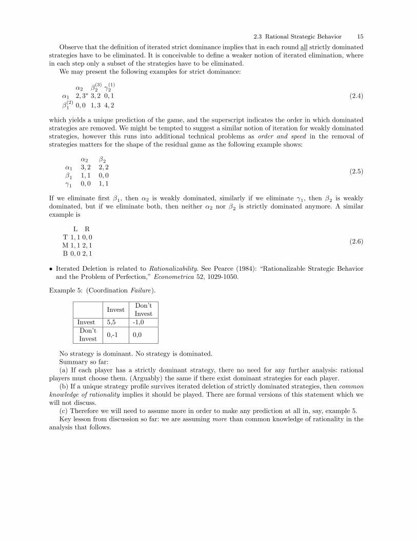
Observe that the de�nition of iterated strict dominance implies that in each round all strictly dominatedstrategies have to be eliminated. It is conceivable to de�ne a weaker notion of iterated elimination, wherein each step only a subset of the strategies have to be eliminated.We may present the following examples for strict dominance:
�2 �(3)2
(1)2
�1 2; 3� 3; 2 0; 1
�(2)1 0; 0 1; 3 4; 2
(2.4)
which yields a unique prediction of the game, and the superscript indicates the order in which dominatedstrategies are removed. We might be tempted to suggest a similar notion of iteration for weakly dominatedstrategies, however this runs into additional technical problems as order and speed in the removal ofstrategies matters for the shape of the residual game as the following example shows:
�2 �2�1 3; 2 2; 2�1 1; 1 0; 0 1 0; 0 1; 1
(2.5)
If we eliminate �rst �1, then �2 is weakly dominated, similarly if we eliminate 1, then �2 is weaklydominated, but if we eliminate both, then neither �2 nor �2 is strictly dominated anymore. A similarexample is
L RT 1; 1 0; 0M 1; 1 2; 1B 0; 0 2; 1
(2.6)
� Iterated Deletion is related to Rationalizability. See Pearce (1984): \Rationalizable Strategic Behaviorand the Problem of Perfection," Econometrica 52, 1029-1050.
Example 5: (Coordination Failure).
InvestDon'tInvest
Invest 5,5 -1,0Don'tInvest
0,-1 0,0
No strategy is dominant. No strategy is dominated.Summary so far:(a) If each player has a strictly dominant strategy, there no need for any further analysis: rational
players must choose them. (Arguably) the same if there exist dominant strategies for each player.(b) If a unique strategy pro�le survives iterated deletion of strictly dominated strategies, then common
knowledge of rationality implies it should be played. There are formal versions of this statement which wewill not discuss.(c) Therefore we will need to assume more in order to make any prediction at all in, say, example 5.Key lesson from discussion so far: we are assuming more than common knowledge of rationality in the
analysis that follows.

3. Nash Equilibrium
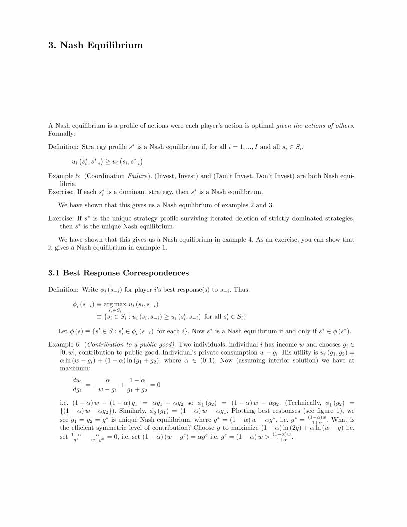
A Nash equilibrium is a pro�le of actions were each player's action is optimal given the actions of others.Formally:
De�nition: Strategy pro�le s� is a Nash equilibrium if, for all i = 1; :::; I and all si 2 Si,
ui�s�i ; s
��i�� ui
�si; s
��i�
Example 5: (Coordination Failure). (Invest, Invest) and (Don't Invest, Don't Invest) are both Nash equi-libria.
Exercise: If each s�i is a dominant strategy, then s� is a Nash equilibrium.
We have shown that this gives us a Nash equilibrium of examples 2 and 3.
Exercise: If s� is the unique strategy pro�le surviving iterated deletion of strictly dominated strategies,then s� is the unique Nash equilibrium.
We have shown that this gives us a Nash equilibrium in example 4. As an exercise, you can show thatit gives a Nash equilibrium in example 1.
3.1 Best Response Correspondences
De�nition: Write �i (s�i) for player i's best response(s) to s�i. Thus:
�i (s�i) � argmaxsi2Si
ui (si; s�i)
� fsi 2 Si : ui (si; s�i) � ui (s0i; s�i) for all s0i 2 Sig
Let � (s) � fs0 2 S : s0i 2 �i (s�i) for each ig. Now s� is a Nash equilibrium if and only if s� 2 � (s�).
Example 6: (Contribution to a public good). Two individuals, individual i has income w and chooses gi 2[0; w], contribution to public good. Individual's private consumption w � gi. His utility is ui (g1; g2) =� ln (w � gi) + (1� �) ln (g1 + g2), where � 2 (0; 1). Now (assuming interior solution) we have atmaximum:
du1dg1
= � �
w � g1+1� �g1 + g2
= 0
i.e. (1� �)w � (1� �) g1 = �g1 + �g2 so �1 (g2) = (1� �)w � �g2. (Technically, �1 (g2) =f(1� �)w � �g2g). Similarly, �2 (g1) = (1� �)w � �g1. Plotting best responses (see �gure 1), wesee g1 = g2 = g
� is unique Nash equilibrium, where g� = (1� �)w � �g�, i.e. g� = (1��)w1+� . What is
the e�cient symmetric level of contribution? Choose g to maximize (1� �) ln (2g) + � ln (w � g) i.e.set 1��ge � �
w�ge = 0, i.e. set (1� �) (w � ge) = �ge i.e. ge = (1� �)w > (1��)w
1+� .
18 3. Nash Equilibrium
See MWG section 11.C for more general discussion of ine�ciency of voluntary public good provision.A more complicated best response correspondence:
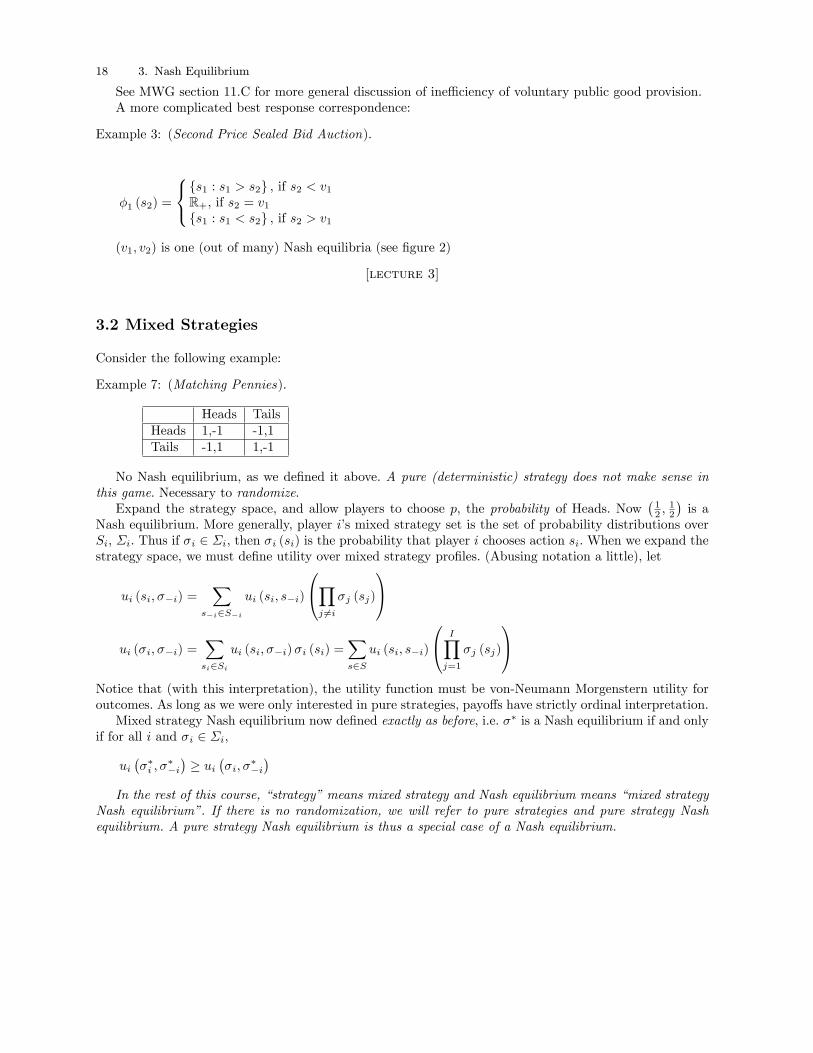
Example 3: (Second Price Sealed Bid Auction).
�1 (s2) =
8<:fs1 : s1 > s2g , if s2 < v1R+, if s2 = v1fs1 : s1 < s2g , if s2 > v1
(v1; v2) is one (out of many) Nash equilibria (see �gure 2)
[lecture 3]
3.2 Mixed Strategies
Consider the following example:
Example 7: (Matching Pennies).
Heads TailsHeads 1,-1 -1,1Tails -1,1 1,-1
No Nash equilibrium, as we de�ned it above. A pure (deterministic) strategy does not make sense inthis game. Necessary to randomize.Expand the strategy space, and allow players to choose p, the probability of Heads. Now
�12 ;
12
�is a
Nash equilibrium. More generally, player i's mixed strategy set is the set of probability distributions overSi, �i. Thus if �i 2 �i, then �i (si) is the probability that player i chooses action si. When we expand thestrategy space, we must de�ne utility over mixed strategy pro�les. (Abusing notation a little), let
ui (si; ��i) =X
s�i2S�i
ui (si; s�i)
0@Yj 6=i�j (sj)
1Aui (�i; ��i) =
Xsi2Si
ui (si; ��i)�i (si) =Xs2S
ui (si; s�i)
0@ IYj=1
�j (sj)
1ANotice that (with this interpretation), the utility function must be von-Neumann Morgenstern utility foroutcomes. As long as we were only interested in pure strategies, payo�s have strictly ordinal interpretation.Mixed strategy Nash equilibrium now de�ned exactly as before, i.e. �� is a Nash equilibrium if and only
if for all i and �i 2 �i,
ui���i ; �
��i�� ui
��i; �
��i�
In the rest of this course, \strategy" means mixed strategy and Nash equilibrium means \mixed strategyNash equilibrium". If there is no randomization, we will refer to pure strategies and pure strategy Nashequilibrium. A pure strategy Nash equilibrium is thus a special case of a Nash equilibrium.

3.3 Existence of Nash Equilibrium: 19
Dominated Strategies Revisited:. Consider the following game:
Left RightUp 4,0 -2,0Middle 0,0 0,0Down -2,0 4,0
Pure strategy \Middle" is not dominated by any pure strategy. But \Middle" is strictly dominated bythe strategy putting probability 1
2 on Left and12 on Right.
3.3 Existence of Nash Equilibrium:
Theorem (Nash 1950) Every �nite action game has at least one Nash equilibrium.
Proof. De�ne � : � ! � as follows. Each mixed strategy can be thought of as a vector and Euclideandistance between mixed strategy vectors can be described in the usual way:
k�0i � �ik =sXsi2Si
(�0i (si)� �i (si))2
Let vi (�0i; �) = ui (�
0i; ��i)� c k�0i � �ik
2(where c > 0)
�i (�) = argmax�0i2�i
vi (�0i; �)
� (�) = f�i (�)gIi=1
Interpretation: � is a \better response" function with quadratic adjustment costs.
1. � is non-empty, compact and convex.2. vi is strictly concave in �
0i (�rst term is linear, and thus concave, second term is negative quadratic,
and thus strictly concave). Thus �i is uniquely de�ned and continuous in �. Thus � is a continuousfunction on �.
3. If �� = � (��), then �� is a Nash equilibrium. Suppose not. Then there exists i and �i 2 �i such that� = ui
��i; �
��i�� ui
���i ; �
��i�> 0. Now:
vi ("�i + (1� ")��i ; ��)� vi (��i ; ��) = "�� c"2 k�i � ��i k2
which is strictly positive for " su�ciently close to zero.
Brouwer's Fixed Point Theorem: Suppose X is a non-empty, compact, convex subset of RN andf : X ! X is continuous. Then f has a �xed point, i.e., there exists x 2 X with x = f(x).Now Nash equilibrium exists by points 1 through 3 above.
� This proof follows Geanakoplos (1996): \Nash and Walras Equilibrium Via Brouwer," Cowles FoundationDiscussion Paper #1131.
Existence with continuous strategy spaces: If payo�s are continuous, then existence is no problem. Withdiscontinuous payo�s, existence is a real problem. Best responses may not be well de�ned. Discontinuouspayo�s arise naturally in economic settings, and cause real problems. They arise naturally in price-settinggames (to be discussed furthers in the next section). We return to this issue at the end of the next section.
20 3. Nash Equilibrium
3.4 Imperfect Competition
Homogenous Good. Assume constant marginal cost c > 0 (with varying marginal cost, entry as-sumptions become crucial; we will return to this later). Demand x (p); assume di�erentiable, non-increasing, strictly decreasing if x (p) > 0, x (p) = 0 for all p � p. This implies inverse demand functionp (q) = min fp : q = x (p)g.Competitive Case. Choose q to maximize q [p� c].Must have pc = c, qc implicitly de�ned by
p (qc) = c
Monopoly. Choose p to maximize pro�ts: x (p) [p� c]Choose q to maximize pro�ts: q [p (q)� c]First Order Condition:
Marginal Revenue = p (q) + qp0 (q) = c = Marginal Cost
Equivalently,
p� cp
= �qp0 (q)
p= �1
�,
where � is the own price elasticity of demand. Let qm solve
p (qm) + qmp0 (qm) = c
and
pm = p (qm)
Observe that pm > pc and qm < qc.
Oligopoly. I �rms
Quantity Competition (\Cournot Competition"). Payo� functions:
�i (q1; :::::; qI) = qi
24p0@ IXj=1
qj
1A� c35
First order condition:
d�idqi
= p
0@ IXj=1
qj
1A+ qip00@ IXj=1
qj
1A� c = 0In a symmetric equilibrium, qi = q for all i (by continuity, a symmetric solution to the �rst order conditionwill exist). So if we write qI = Iq for total quantity produced in oligopoly, we have qI solving
p�qI�+1
IqIp0
�qI�= c.
Thus qm = q1 and qc = q1. Exercise: how does qI vary as I increases....
3.4 Imperfect Competition 21
Price Competition (\Bertrand Competition"). Payo� Functions:
�i (p1; :::::; pI) =
(1
#fi:pi=pgx�p� �p� c
�, if pi = p
0, if pi > p
where
p = minipi
A pure strategy pro�le is a Nash equilibrium (for any I � 2) if and only if p = c and at least two �rmschoose price c. Clearly, any such strategy pro�le is an equilibrium (no incentive to deviate). Let's see whatgoes wrong in all other possible cases.(i) p < c. Any �rm setting price equal to p is making losses and has an incentive to increase price.(ii) p1 = c and pi > c for all i 6= 1. Firm 1 has incentive to increase price to c+ " (for some " su�ciently
small).(iii) p > c and let n be the number of �rms setting pi = p. If n 6= I, any �rm not setting pi = p has an
incentive to deviate to pi = p� " (increasing pro�ts from 0 to�p� "� c
�x�p� "
�). If n = I, any �rm has
an incentive to deviate to pi = p� " (increasing pro�ts from 1I
�p� c
�x�p�to�p� "� c
�x�p� "
�).
As an exercise, show that this is also true for mixed strategies.
3.4.1 An Existence Problem
Consider the price competition model with two �rms, but di�erent costs: c1 < c2. No equilibrium exists.Pure strategy argument. First suppose that they choose the same price p. If p < c2, �rm 2 loses money;
if p > c1, �rm 1 increases pro�ts by charging p � ". Now suppose that �rms choose di�erent prices. The�rm choosing the lower price can increase pro�ts by raising prices by ".Let p
1and p
2be the lowest price chosen by the two �rms respectively. First suppose that p
1= p
2= p.
As before, if p < c2, �rm 2 loses money; if p > c1, �rm 1 increases pro�ts by charging p� ". Now supposethat p
16= p
2. As before, the �rm with the lower lowest price can increase pro�ts by raising prices by ".
� See Reny (1999): \On the Existence of Pure and Mixed Strategy Nash Equilibria in DiscontinuousGames," Econometrica 67, 1029-1056.
[lecture 4]
3.4.2 Reconciling quantity and price competition
The role of capacity constraints in Cournot.
3.4.3 Imperfect Substitutes: Monopolistic Competition and the Dixit/Stiglitz model
Goods are imperfect substitutes. Each �rm has monopoly in own product.Consumer demand over J products:
u (m;x1; ::::; xJ) = G
0@ JXj=1
f (xj)
1A+mwhere G (�) and f (�) are concave. Setting the price of the numeraire good to be 1, we get �rst orderconditions

22 3. Nash Equilibrium
G0
0@ JXj=1
f (xj)
1A f 0 (xj) = pjThis gives a demand function xj (p1; :::::; pJ). Each �rm maximizes (pj � c)xj (p1; :::::; pJ)Each �rm acts like a monopolist, setting
xj + pjdxjdpj
= cdxjdpj
pj � cpj
= � xj
pjdxjdpj
Life becomes even simpler if there are a continuum of products:
u (m;x) = G
Zj2[0;1]
f (xj) dj
!+m
where G (�) and f (�) are concave. Setting the price of the numeraire good to be 1, we get �rst orderconditions
G0
Zj2[0;1]
f (xj) dj
!f 0 (xj) = pj
Set x =Rj2[0;1] f (xj) dj. Now we can look at demand function xj (pj ; x) � [f
0]�1 �pj
x
�. Each �rm maximizes
(pj � c)xj (pj ; x)Each �rm acts like a monopolist, setting
xj + pjdxjdpj
= cdxjdpj
By symmetry, we are looking for a level of output x and price p such that
G0 (x) f 0 (x) = p
x+ pdxjdpj
= cdxjdpj
[lecture 9]
3.5 Entry and the Competitive Limit 12.E, 12.F
U -shaped average cost curve: �xed cost of entry K > 0; variable cost function c (q), with c (0) = 0,c0 (�) > 0 and c00 (q) > 0. Demand �x (p) (where � parameterizes the size of the market); inverse demandp�q�
�. Assume c (�), x (�) and thus p (�) are twice continuously di�erentiable. Let
c = minq
K + c (q)
q
with q the cost minimizing quantity. See �gure 13. Recall from Econ 101 that we must have c0�q�= c.
This is because the �rst order condition of the average cost minimization is
�K + c (q)
q2+c0 (q)
q= 0.
3.5 Entry and the Competitive Limit 12.E, 12.F 23
3.5.1 Competitive Case MWG 10.F
We are looking for equilibrium (J�; p�; q�)(i) Supply Equals Demand: �x (p�) = J�q�
(ii) Optimal Output Choice:
q� = argmaxq
p�q � c (q)
i.e., p� = c0 (q�)
(iii) Zero Pro�t (Free Entry) Condition:
p�q� � c (q�)�K = 0
Note: there is an \integer problem." But if there is a solution, we must have q� = q, p� = c and
J� = �x(c)q . If p� < c, �rms must make losses. If p� > c, �rms must make strictly positive pro�ts, violating
the zero pro�t condition.
Ignoring the integer problem, there is \e�cient entry," i.e., (J�; p�; q�) =��x(c)q ; c; q
�maximizes
JqZ0
p
�t
�
�dt� JK � Jc (q)
since total output is produced at minimum cost (c) and output would maximize consumer surplus atconstant marginal cost c.
3.5.2 Modelling Entry 12.E
Two stage game between in�nite number of identical potential entrants.Stage 1: each �rms enters, or not. Cost of entry: K > 0.Stage 2: Cournot competition with inverse demand function p
�q�
�.
Suppose that there is a unique symmetric Nash equilibrium of the Cournot game with each �rm pro-ducing output qJ and each �rm earning operating pro�ts �J (i.e., ignoring sunk entry cost). Also assumethat �J is decreasing in J . Then the unique equilibrium (J�; p�; q�) is characterized by three properties:(i) Supply Equals Demand: �x (p�) = J�q�
(ii) Nash Output Choice:
q� = argmaxq
p
�(J� � 1) q� + q
�
�q � c (q)
i.e., p
�J�q�
�
�+1
�p0�J�q�
�
�q� = c0 (q�)
(iii) Entry Condition:
��J � K, ��J+1 � K
Clearly, there is ine�ciencies because the price is above marginal cost. But we can ask if the number of�rms entering in equilibrium is e�cient. Write Jeff for the e�cient number of �rms in the industry.Suppose that (1) each �rm's output is decreasing in the number of entrants (qJ is decreasing in J),
\business stealing" ; (2) total output is increasing in the number of entrants (JqJ is increasing in J). ThenJ� � Jeff � 1.Negative externality from business stealing tends to create excess entry. An example of too little entry
is when optimal number is 1 and no �rms enter.
24 3. Nash Equilibrium
3.5.3 The Competitive Limit 12.F
Let p� be the equilibrium price.Proposition: as �!1, p� ! c.
[lecture 10]
Proof. We have sequence of equilibria (J�; p�; q�).Step 1: let �� (Q) be a �rm's best response when total output of other �rms is Q; for su�ciently large
�, �� (�) is decreasing.For su�ciently high Q, best response is to produce nothing. At interior solution, we have FOC:
p
�Q+ �� (Q)
�
�+1
�p0�Q+ �� (Q)
�
��� (Q) = c
0 (�� (Q))
Totally di�erentiating w.r.t. Q, we obtain8>>><>>>:1�p
0�Q+��(Q)
�
� �1 + �0� (Q)
�+ 1�2 p
00�Q+��(Q)
�
� �1 + �0� (Q)
��� (Q)
+ 1�p
0�Q+��(Q)
�
��0� (Q)
9>>>=>>>; = c00 (�� (Q))�0� (Q)
Thus
�0� (Q) =�z (Q)
z (Q) + 1�p
0�Q+��(Q)
�
�� c00 (�� (Q))
where
z (Q) =1
�p0�Q+ �� (Q)
�
�+1
�2p00�Q+ �� (Q)
�
��� (Q)
We will show that z (Q) < 0. But Q+��(Q)� cannot be higher than the choke price.Step 2: Must have q�J� � �x (c)� q. If not, a �rm could enter and produce q. The price will be above
c, implying that entry pays.Step 3: Now observe that
jp� � cj � p
��x (c)� q
�
�� p
��x (c)
�
�= p
�x (c)�
q
�
�� p (x (c))
! 0, as �!1
Part II
Dynamic Games of Complete Information

4. Perfect Information Games:
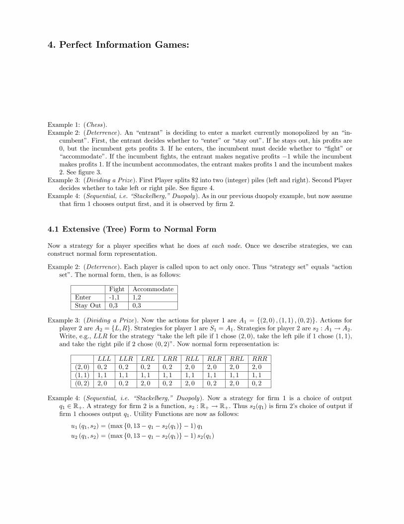
Example 1: (Chess).Example 2: (Deterrence). An \entrant" is deciding to enter a market currently monopolized by an \in-
cumbent". First, the entrant decides whether to \enter" or \stay out". If he stays out, his pro�ts are0, but the incumbent gets pro�ts 3. If he enters, the incumbent must decide whether to \�ght" or\accommodate". If the incumbent �ghts, the entrant makes negative pro�ts �1 while the incumbentmakes pro�ts 1. If the incumbent accommodates, the entrant makes pro�ts 1 and the incumbent makes2. See �gure 3.
Example 3: (Dividing a Prize). First Player splits $2 into two (integer) piles (left and right). Second Playerdecides whether to take left or right pile. See �gure 4.
Example 4: (Sequential, i.e. \Stackelberg," Duopoly). As in our previous duopoly example, but now assumethat �rm 1 chooses output �rst, and it is observed by �rm 2.
4.1 Extensive (Tree) Form to Normal Form
Now a strategy for a player speci�es what he does at each node. Once we describe strategies, we canconstruct normal form representation.
Example 2: (Deterrence). Each player is called upon to act only once. Thus \strategy set" equals \actionset". The normal form, then, is as follows:
Fight AccommodateEnter -1,1 1,2Stay Out 0,3 0,3
Example 3: (Dividing a Prize). Now the actions for player 1 are A1 = f(2; 0) ; (1; 1) ; (0; 2)g. Actions forplayer 2 are A2 = fL;Rg. Strategies for player 1 are S1 = A1. Strategies for player 2 are s2 : A1 ! A2.Write, e.g., LLR for the strategy \take the left pile if 1 chose (2; 0), take the left pile if 1 chose (1; 1),and take the right pile if 2 chose (0; 2)". Now normal form representation is:
LLL LLR LRL LRR RLL RLR RRL RRR(2; 0) 0; 2 0; 2 0; 2 0; 2 2; 0 2; 0 2; 0 2; 0(1; 1) 1; 1 1; 1 1; 1 1; 1 1; 1 1; 1 1; 1 1; 1(0; 2) 2; 0 0; 2 2; 0 0; 2 2; 0 0; 2 2; 0 0; 2
Example 4: (Sequential, i.e. \Stackelberg," Duopoly). Now a strategy for �rm 1 is a choice of outputq1 2 R+. A strategy for �rm 2 is a function, s2 : R+ ! R+. Thus s2(q1) is �rm 2's choice of output if�rm 1 chooses output q1. Utility Functions are now as follows:
u1 (q1; s2) = (max f0; 13� q1 � s2(q1)g � 1) q1u2 (q1; s2) = (max f0; 13� q1 � s2(q1)g � 1) s2(q1)

28 4. Perfect Information Games:
4.1.1 Nash Equilibria
Example 3: (Dividing a Prize). Player 2's Best Responses:
1's strategy 2's best response(2; 0) fLLL;LLR;LRL;LRRg(1; 1) fLLL;LLR;LRL;LRR;RLL;RLR;RRL;RRRg(2; 0) fLLR;LRR;RLR;RRRg
Player 1's Best Responses:
2's strategy 1's best responseLLL (0; 2)LLR (1; 1)LRL (0; 2)LRR (1; 1)RLL (2; 0), (0; 2)RLR (2; 0)RRL (2; 0), (0; 2)RRR (2; 0)
Nash equilibria: f(1; 1); LLRg and f(1; 1) ; LRRg.
4.1.2 Backward Induction and Credible Threats: G 2.1.A, 2.1.D; MWG 9.B
Example 2: (Deterrence). Two Nash equilibria: (Enter, Accommodate) and (Stay Out, Fight).
But second equilibrium is based on an incredible threat.
De�nition: A backward induction equilibrium of a perfect information game is a strategy pro�le where eachplayer's strategy is optimal at every node given that he expects others to follow equilibrium strategiesin the future.
(Enter, Accommodate) is a backward induction equilibrium of the deterrence game.
Example 3: (Dividing a Prize). Backward Induction equilibria are Nash equilibria, f(1; 1) ; LLRg andf(1; 1) ; LRRg.
Proposition: In all �nite horizon perfect information games: (1) there exists a pure strategy backwardsinduction equilibrium; (2) every backward induction equilibrium is a Nash equilibrium; (3) if the gamehas no ties, there is a unique backward induction equilibrium; (4) if the game is \two player constantsum", all backward induction equilibria give the same payo�s.
Example 5: (Hex ). See �gure 5.
[lecture 5]
Example 4: (Sequential Duopoly). Let us �nd backward induction equilibrium. Suppose the �rst �rmchooses output q1. Firm 2's pro�ts are:
�2 (q1; q2) = (max f0; 13� q1 � q2)g � 1) q2
4.3 Subgame Perfection: 29
This is maximized by setting q2 = max�0; 6� q1
2
. Thus �rm 2's strategy is s2(q1) = max
�0; 6� q1
2
.
Now let us calculate �rm 1's pro�ts anticipating that �rm 2 will use an optimal strategy.
If q1 � 12,�1 (q1) =
�max
n0; 13� q1 �max
n0; 6� q1
2
oo� 1�q1
=�12� q1 �
�6� q1
2
��q1
=�6� q1
2
�q1
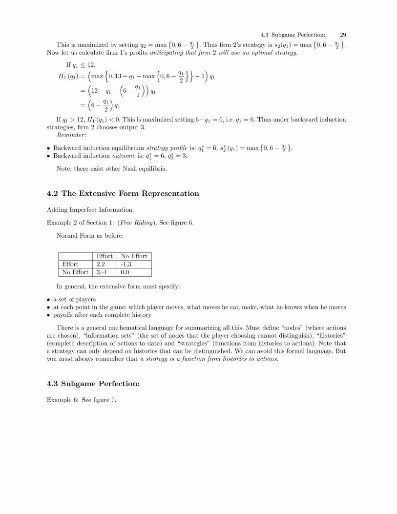
If q1 > 12, �1 (q1) < 0. This is maximized setting 6�q1 = 0, i.e. q1 = 6. Thus under backward inductionstrategies, �rm 2 chooses output 3.Reminder :
� Backward induction equilibrium strategy pro�le is: q�1 = 6, s�2 (q1) = max
�0; 6� q1
2
.
� Backward induction outcome is: q�1 = 6, q�2 = 3.
Note: there exist other Nash equilibria.
4.2 The Extensive Form Representation
Adding Imperfect Information.
Example 2 of Section 1: (Free Riding). See �gure 6.
Normal Form as before:
E�ort No E�ortE�ort 2,2 -1,3No E�ort 3,-1 0,0
In general, the extensive form must specify:
� a set of players� at each point in the game: which player moves, what moves he can make, what he knows when he moves� payo�s after each complete history
There is a general mathematical language for summarizing all this. Must de�ne \nodes" (where actionsare chosen), \information sets" (the set of nodes that the player choosing cannot distinguish), \histories"(complete description of actions to date) and \strategies" (functions from histories to actions). Note thata strategy can only depend on histories that can be distinguished. We can avoid this formal language. Butyou must always remember that a strategy is a function from histories to actions.
4.3 Subgame Perfection:
Example 6: See �gure 7.
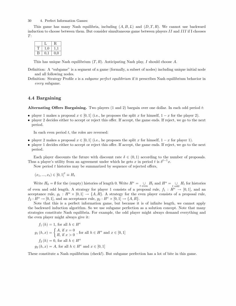
30 4. Perfect Information Games:
This game has many Nash equilibria, including (A;B;L) and (D;T;R). We cannot use backwardinduction to choose between them. But consider simultaneous game between players II and III if I choosesT :
L RT 1,0 1,1B 0,1 0,0
This has unique Nash equilibrium (T;R). Anticipating Nash play, I should choose A.
De�nition: A \subgame" is a segment of a game (formally, a subset of nodes) including unique initial nodeand all following nodes.
De�nition: Strategy Pro�le s is a subgame perfect equilibrium if it prescribes Nash equilibrium behavior inevery subgame.
4.4 Bargaining
Alternating O�ers Bargaining. Two players (1 and 2) bargain over one dollar. In each odd period t:
� player 1 makes a proposal x 2 [0; 1] (i.e., he proposes the split x for himself, 1� x for the player 2).� player 2 decides either to accept or reject this o�er. If accept, the game ends. If reject, we go to the nextperiod.
In each even period t, the roles are reversed:
� player 2 makes a proposal x 2 [0; 1] (i.e., he proposes the split x for himself, 1� x for player 1).� player 1 decides either to accept or reject this o�er. If accept, the game ends. If reject, we go to the nextperiod.
Each player discounts the future with discount rate � 2 (0; 1) according to the number of proposals.Thus a player's utility from an agreement under which he gets x in period t is �t�1x.Now period t histories may be summarized by sequence of rejected o�ers,
(x1; :::; xt) 2 [0; 1]t � Ht
Write H0 = ; for the (empty) histories of length 0. Write He = [t even
Ht and Ho = [
t oddHt for histories
of even and odd length. A strategy for player 1 consists of a proposal rule, f1 : He ! [0; 1], and an
acceptance rule, g1 : Ho � [0; 1] ! fA;Rg. A strategy for the even player consists of a proposal rule,
f2 : Ho ! [0; 1], and an acceptance rule, g2 : H
e � [0; 1]! fA;Rg.Note that this is a perfect information game, but because it is of in�nite length, we cannot apply
the backward induction algorithm. So we use subgame perfection as a solution concept. Note that manystrategies constitute Nash equilibria. For example, the odd player might always demand everything andthe even player might always give it:
f1 (h) = 1, for all h 2 He
g1 (h; x) =
�A, if x = 0R, if x > 0
, for all h 2 Ho and x 2 [0; 1]
f2 (h) = 0, for all h 2 Ho
g2 (h; x) = A, for all h 2 He and x 2 [0; 1]
These constitute a Nash equilibrium (check!). But subgame perfection has a lot of bite in this game.

4.5 Nash Bargaining Problem: MWG 22.E 31
Theorem: The following strategies are the unique subgame perfect Nash equilibrium strategies:
f1 (h) =1
1 + �, for all h 2 He
g1 (h; x) =
�A, if x � 1
1+�
R, if x > 11+�
, for all h 2 Ho and x 2 [0; 1]
f2 (h) =1
1 + �, for all h 2 Ho
g2 (h; x) =
�A, if x � 1
1+�
R, if x > 11+�
, for all h 2 He and x 2 [0; 1]
Idea of Proof. Checking that these are SPNE is straightforward. Consider any player about to makea proposal. Discounted equilibrium payo� from that point on is 1
1+� . A lower proposal would be accepted,
giving a lower payo�. A higher proposal would be rejected, giving payo� at most �2
1+� (the discounted valueof what the proposer would be o�ered in the next period). Now consider a player about to accept or reject.Rejecting gives a payo� of �
1+� (the discounted value of being the proposer in the next period). Thereforeis rational to accept exactly o�ers that give this amount.
[lecture 6]
Harder part is showing uniqueness. Let x and x be the highest and lowest (formally, supremum andin�mum) payo� received by the odd player in any SPNE of the in�nite game; let y and y be the highestand lowest (formally, supremum and in�mum) payo� received by the even player in any SPNE. Note thatbecause of the stationarity of the game, x and x are also the highest and lowest payo� (discounted fromthat point on) received by either player after any history in any SPNE of the continuation; similarly, y andy are the highest and lowest SPNE of the player accepting or rejecting.Claim 1. (i) y � �x and (ii) y � �x. For (i), observe that a player would always accept any o�er that
gave strictly more than �x (the most he could conceivably get by rejecting); so the proposer would nevero�er strictly more that �x. For (ii), rejection guarantees a player at least �x.Claim 2. x � 1��x. Same argument as in claim 1, part (i): a player would always accept any o�er that
gave strictly more than �x (the most he could conceivably get by rejecting); so the proposer is guaranteed1� �x.Claim 3. x � max (1� �x; �y) � max
�1� �x; �2x
�. Proposer attains maximum payo� either by getting
current proposal accepted (giving at most 1� �x) or by getting it rejected (giving at most �y). The secondinequality follows from claim 1, part (i).Claim 4. x � 1 � �x. If �2x � 1 � �x, then claim 3 ) x � �2x ) x � �2x ) x = 0 )(by claim 2)
x = 1, a contradiction. So �2x < 1� �x, and claim 4 follows from claim 3.Thus
x � 1� �x, by claim 4
� 1� � (1� �x) , by claim 2
� 1� � + �2xThus x � 1��
1��2 =11+� . By claim 2, x � 1� �x � 1� �
1+� =11+� . So x = x =
11+� . Combined with claim 1,
we have y = y = �1+� . It remains only to verify that the strategies described above are the only ones giving
these unique equilibrium payo�s (check!).
4.5 Nash Bargaining Problem: MWG 22.E
Two individuals. Feasible outcomes: F � <2; assume F is closed, convex set. A point x � (x1; x2) 2 F isinterpreted as a utility assignment to the two players. Disagreement point v � (v1; v2). Utility assignment
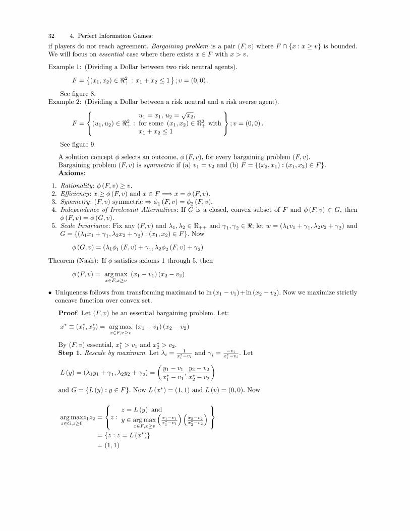
32 4. Perfect Information Games:
if players do not reach agreement. Bargaining problem is a pair (F; v) where F \ fx : x � vg is bounded.We will focus on essential case where there exists x 2 F with x > v.
Example 1: (Dividing a Dollar between two risk neutral agents).
F =�(x1; x2) 2 <2+ : x1 + x2 � 1
; v = (0; 0) :
See �gure 8.Example 2: (Dividing a Dollar between a risk neutral and a risk averse agent).
F =
8<:(u1; u2) 2 <2+ : u1 = x1, u2 =px2,
for some (x1; x2) 2 <2+ withx1 + x2 � 1
9=; ; v = (0; 0) :See �gure 9.
A solution concept � selects an outcome, � (F; v), for every bargaining problem (F; v).Bargaining problem (F; v) is symmetric if (a) v1 = v2 and (b) F = f(x2; x1) : (x1; x2) 2 Fg.Axioms:
1. Rationality : � (F; v) � v.2. E�ciency : x � � (F; v) and x 2 F =) x = � (F; v).3. Symmetry : (F; v) symmetric ) �1 (F; v) = �2 (F; v).4. Independence of Irrelevant Alternatives: If G is a closed, convex subset of F and � (F; v) 2 G, then� (F; v) = � (G; v).
5. Scale Invariance: Fix any (F; v) and �1; �2 2 <++ and 1; 2 2 <; let w = (�1v1 + 1; �2v2 + 2) andG = f(�1x1 + 1; �2x2 + 2) : (x1; x2) 2 Fg. Now
� (G; v) = (�1�1 (F; v) + 1; �2�2 (F; v) + 2)
Theorem (Nash): If � satis�es axioms 1 through 5, then
� (F; v) = argmaxx2F;x�v
(x1 � v1) (x2 � v2)
� Uniqueness follows from transforming maximand to ln (x1 � v1)+ln (x2 � v2). Now we maximize strictlyconcave function over convex set.
Proof. Let (F; v) be an essential bargaining problem. Let:
x� � (x�1; x�2) = argmaxx2F;x�v
(x1 � v1) (x2 � v2)
By (F; v) essential, x�1 > v1 and x�2 > v2.
Step 1. Rescale by maximum. Let �i =1
x�i�viand i =
�vix�i�vi
. Let
L (y) = (�1y1 + 1; �2y2 + 2) =
�y1 � v1x�1 � v1
;y2 � v2x�2 � v2
�and G = fL (y) : y 2 Fg. Now L (x�) = (1; 1) and L (v) = (0; 0). Now
argmaxz2G;z�0
z1z2 =
8<:z : z = L (y) andy 2 argmaxx2F;x�v
�x1�v1x�1�v1
��x2�v2x�2�v2
� 9=;= fz : z = L (x�)g= (1; 1)
4.5 Nash Bargaining Problem: MWG 22.E 33
Thus G � E =�z 2 <2 : z1 + z2 � 2
.
Step 2. E is symmetric. So by E�ciency and Symmetry: � (E; (0; 0)) = (1; 1).Step 3. Independence of Irrelevant Alternatives: � (G; (0; 0)) = � (E; (0; 0)) = (1; 1).Step 4. Scale Invariance: L (� (F; v)) = � (G; (0; 0)) = (1; 1); so � (F; v) = x�.In example 1, the Nash solution is
�12 ;
12
�.
In example 2, the e�ciency frontier is the set of points where u1 = 1� (u2)2; thus the Nash product (asa function of u2) is u2
h1� (u2)2
i. This is maximized where u2 =
1p3and thus u1 =
23 . This utility pro�le
corresponds to player 1 receiving cash of 13 , and player 2 receiving cash of23 .
4.5.1 The \Nash Program": Alternating O�ers and the Nash Bargaining Solution
� See Myerson (1991): Game Theory: Analysis of Con ict, chapter 8, for an excellent discussion of thismaterial.
Consider the alternative o�ers game where the proposer picks a point x = (x1; x2) 2 F , and the otherplayer accepts or rejects. If we analyze this game with
F =�(x1; x2) 2 <2+ : x1 + x2 � 1
; v = (0; 0) :
we get essentially the analysis we had before (in principle, players could propose an ine�cient point, butthey would not do so in equilibrium). Note that as � ! 1, the unique equilibrium gave each player 1
2 , i.e.,the Nash bargaining solution.In fact, essentially the same argument goes through when the alternative o�ers game is applied to any
bargaining problem; i.e., there is a unique subgame perfect equilibrium where each player's strategy isstationary (i.e., is independent of past history). One can show that as � ! 1, this unique solution giveseach player the Nash bargaining solution.
[lecture 7]


5. Repeated Games and Folk Theorems:
Example 8: (Twice Repeated Free Riding Game). See �gure 10.
Strategy for each player must specify �ve things: what to do in �rst period and what to do in secondperiod after each of the 4 histories (EE;EN;NE;NN). Thus we could write \EEENN" for player 2'sstrategy \play E in the �rst period; play E in the second period if player 1 plays E in the �rst period; playN in the second period otherwise"This game has a unique subgame perfect Nash equilibrium: (NNNNN;NNNNN), i.e., each player
makes no e�ort after any history.
Theorem: If a stage game has a unique Nash equilibrium, then the unique subgame perfect Nash equilibriumof the �nitely repeated stage game has each player playing according to the unique stage game Nashequilibrium after every history.
However, it is not true in general that repeated game must involve stage game Nash equilibria only.
Example 9: Suppose the following stage game is repeated twice.
L M RL 1,1 5,0 1,0M 0,5 4,4 0,0R 0,1 0,0 3,3
Action L strictly dominates action M for both players. So the game has two Nash equilibria: (L;L)and (R;R). But consider the following strategy for either player:
� Play M in the �rst period. If (M;M) is played in the �rst period, play R in the second period. Afterany other �rst period history, play L.
Formally, the above strategy is let (M;f), where f : fL;M;Rg2 ! fL;M;Rg and
f (h) =
�R, if h = (M;M)L, if h 6= (M;M)
If both players choose this strategy, we have a subgame perfect Nash equilibrium. To see why, �rst notethat after every �rst period history, players' strategies imply that a stage game Nash equilibrium is played.Now consider the �rst period. If player 1 deviates to L in the �rst period, his maximum payo� is 5 + 1.If he deviates to R, his maximum payo� is 0 + 1. But following his equilibrium strategy and choosing Mgives 4 + 3.
36 5. Repeated Games and Folk Theorems:
5.1 In�nitely Repeated Games
Stage game repeated in�nite number of times. Payo�s discounted with discount rate �.Formal Description:Stage Game: players 1; ::; I; action sets A1; ::; AI ; stage game payo� functions g1; :::; gI ; where gi : A!
R+ and A = A1�::�AI . Period t histories: Ht = At�1. Histories H = [t�1Ht. An (in�nitely repeated game)
strategy for player i is a function si : H ! A. Write Si for the set of such strategies and S = S1 � ::� SI .Write a (s) 2 A1 for the in�nite history generated by strategy pro�le s, i.e., a (s) =
�a1 (s) ; a2 (s) ; ::::
�where
a1 (s) = fsi (;)gIi=1a2 (s) =
�si�a1 (s)
�Ii=1
a3 (s) =�si�a1 (s) ; a2 (s)
�Ii=1
etc....
Now player i's payo�s function is ui : S ! R, where
ui (s) = (1� �)1Xt=1
�t�1gi�at (s)
�Note the normalization: if player i's one period payo� is x every period, his in�nitely repeated game
payo� is (1� �)1Pt=1�t�1x = x.
Fact: (The One Shot Deviation Principle) In a discounted in�nitely repeated �nite action game, strategypro�le s is a subgame perfect Nash equilibrium if and only if no one shot deviation pays.
Strategy s0i is a one-shot deviation from si if s0i (h
t) = s0i (ht) for all ht 6= eht.
Intuition: For �nite action game, payo�s are bounded, say by M . Suppose deviation s0i gives expectedgain " at some node. then there exists a T -shot deviation, s00i which gives at least "��
TM . For T su�cientlylarge, this is positive. But if a \T -shot" deviation gives a positive gain, then there must exist a last deviationwhich gives a strictly positive gain....
5.2 Folk Theorems
Example 10: (In�nitely Repeated Partnership Game). Recall the stage game.
E�ort (E) No E�ort (N)E�ort (E) 2,2 -1,3No E�ort (N) 3,-1 0,0
Consider the following trigger strategy :
� Play E in the �rst period� Play E after every history in which E has always been played by both players in every period in thepast
� Play N after every history in which either player has ever played N
5.2 Folk Theorems 37
Does each player following this trigger strategy constitute a subgame perfect Nash equilibrium? Wemust check for every one shot deviation. This sounds hard. But there are only two types of deviation tocheck: on and o� the equilibrium path.
� On the equilibrium path, following the trigger strategy (i.e., playing E) gives payo� stream (2; 2; ::::),and thus utility 2. A one shot deviation (i.e., playing N) gives payo� stream (3; 0; 0::::), and thus utility3 (1� �). This pays if and only if � < 1
3 .� O� the equilibrium path, following the trigger strategy (i.e., playing N) gives payo� stream (0; 0; ::::),and thus utility 0. A one shot deviation (i.e., player E) gives payo� stream (�1; 0; 0::::), and thus utility� (1� �). This never pays.
Thus subgame perfect Nash equilibrium exactly if � � 13 .
[lecture 8]
Fix stage game (A; g).
� Feasible Payo�s:
F = conv�x 2 RI : xi = gi (a) for some a 2 A
.
See �gure 11 for the feasible payo�s for the partnership game.Write G (�) for an in�nitely repeated game with discount rate �, and let a� be a pure strategy Nash
equilibrium of the stage game. Then
Theorem: For any v 2 F with v � g (a�), there exists � < 1; such that for all � � �, G (�) has a subgameperfect Nash equilibrium with payo�s arbitrarily close to v.
Proof. First suppose there exists a with g (a) = v. Consider the following strategy:
si�ht�=
8<:ai, if t = 1ai, if ht = (a; ::; a)
a�i , otherwise
Each to check no incentive to deviate o� the equilibrium path. No incentive to deviate on the equilibriumpath if
gi (a) � (1� �) maxai2Ai
gi (ai; a�i) + �gi (a�)
for all i. Rewriting:
� [gi (a)� gi (a�)] � (1� �)�maxai2Ai
gi (ai; a�i)� gi (a)�
i.e.,
� � � = maxi
�maxai2Ai
gi (ai; a�i)� gi (a)�
�maxai2Ai
gi (ai; a�i)� gi (a)�+ [gi (a)� gi (a�)]
In the general case (where there is not a pure strategy supporting payo� v) �nd a sequence of actionpro�les
�a1; a2; ::::; aI
�such that

38 5. Repeated Games and Folk Theorems:
v =1
N
NXn=1
g (an)
(can always do this if v is a vector of rational numbers; if v includes irrational numbers, we can approximateit arbitrarily closely). Now consider the following strategy:
si�ht�=
�ani , if t = n;N + n;N + 2n; ::::and ht =
�a1; a2; ::; aN ; a1; :::
�a�i , otherwise
Payo� under this strategy pro�le is
1� �1� �N
NXn=1
�n�1g (an)
As � ! 1, this expression tends to v. Now a similar (but messier argument) can establish a lower bound of� for this to be an equilibrium.In the repeated partnership game, this theorem essentially characterizes the set of all SPNE, since
clearly no player can be forced below 0 payo�. In general, one can often do better than Nash reversion.Here is an example. Consider again the in�nitely repeated duopoly game. For simplicity, we'll ignore thenon-negativity constraint on prices. Thus the stage game payo�s are gi (a1; a2) = ai (12� a1 � a2).Question 1: For which � does trigger strategy reverting to Cournot output support collusive output?
[Trigger strategy is: (i) produce 3 in the �rst round; (ii) produce 3 if (3; 3) was always played in the past; (iii)produce 4 if either player ever produced anything other than 3 in the past.] Trigger strategies is equilibriumif � � 9
17 .Question 2: Doing better than trigger strategies. Consider the following \stick-and-carrot" strategies.
� Produce 3 in the �rst period.� Produce 3 if either both �rms produced 3 in the previous period or both �rms produced y in the previousperiod.
� Otherwise, produce y.where y 6= 3 and y 6= 4.Suppose � = 1
2 <917 . For what values of y is this an equilibrium? Now we have:
Collusive Pro�t = 3 (12� 3� 3) = 18
Maximum Collusive Deviation Pro�t =81
4Punishment Pro�t = y (12� 2y)
Maximum Punishment Deviation Pro�t = maxqq (12� y � q)
=�6� y
2
��12� y �
�6� y
2
��=�6� y
2
�2Equilibrium path gives: (18; 18; :::). Best deviation gives
�814 ; y (12� 2y) ; 18; 18; :::
�. So no incentive to
deviate from equilibrium path if:
1
2(18� y (12� 2y)) � 81
4� 18
i.e., 36� 24y + 4y2 � 81� 72i.e., 4y2 � 24y + 27 � 0
i.e., (2y � 3) (2y � 9) � 0
i.e., y � 3
2or y � 9
2

5.2 Folk Theorems 39
\Accepting punishment" gives: (y (12� 2y) ; 18; 18; :::). Best deviation gives:��6� y
2
�2; y (12� 2y) ; 18; 18; :::
�.
So no incentive to deviate from punishment if:
1
2(18� y (12� 2y)) �
�6� y
2
�2� y (12� 2y)
i.e., 18 � 2�6� y
2
�2� y (12� 2y)
i.e., 18 � 72� 12y + y2
2� 12y + 2y2
i.e., 0 � 54� 24y +�5
2
�y2
i.e., 5y2 � 48y + 108 � 0i.e., (5y � 18) (y � 6) � 0
i.e.,18
5� y � 6
Combining these conditions, we require 92 � y � 6.
The set of feasible payo�s for the in�nitely repeated game is in fact F = f(v1; v2) : v1 + v2 � 36g (see�gure 12). One can show that any payo� in the feasible set where each player gets strictly more than 0 canbe supported in subgame perfect Nash equilibriumThe general result is:
� Minmax payo�:
vi = min��i2��i
max�i2�i
gi (ai; a�i)
SIR =�x 2 RI : xi > vi for all i
Folk Theorem: Suppose F \ SIR has non-empty interior. Then for all x 2 F \ SIR, there exists �� < 1,
such that if � � ��, the in�nitely repeated game has a subgame perfect Nash equilibrium where eachplayer's equilibrium payo� is xi.
� For survey of such \Repeated Games with Perfect Monitoring", see Pearce (1992): \Repeated Games: Co-operation and Rationality," in Advances in Economic Theory: Sixth World Congress Vol. 1, edited by J.-J.La�ont. Cambridge: Cambridge University Press. A large literature also looks at \Repeated Games withImperfect Private Monitoring," where players observe imperfect (but public) signals of others' past ac-tions; some key contributions are Abreu, Pearce and Stacchetti (1990). \Towards a Theory of DiscountedRepeated Games with Imperfect Monitoring," Econometrica 58, 1041-1063; and Fudenberg, Levine andMaskin (1994). \The Folk Theorem with Imperfect Public Information." There is a also a budding litera-ture on \Repeated Games with Private Monitoring" dealing with settings where players do not know whatsignals others have observed about their past actions. Many of the key papers in this area were includedin a recent Cowles Foundation conference, see http://cowles.econ.yale.edu/conferences/cfmt2000.htm.

Part III
Static Games of Incomplete Information

43
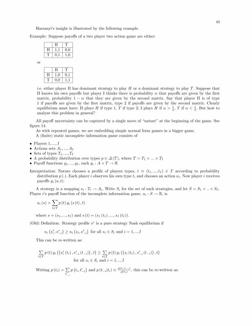
Harsanyi's insight is illustrated by the following example.
Example: Suppose payo�s of a two player two action game are either:
H TH 1,1 0,0T 0,1 1,0
or
H TH 1,0 0,1T 0,0 1,1
i.e. either player II has dominant strategy to play H or a dominant strategy to play T . Suppose thatII knows his own payo�s but player I thinks there is probability � that payo�s are given by the �rstmatrix, probability 1 � � that they are given by the second matrix. Say that player II is of type1 if payo�s are given by the �rst matrix, type 2 if payo�s are given by the second matrix. Clearlyequilibrium must have: II plays H if type 1, T if type 2; I plays H if � > 1
2 , T if � <12 . But how to
analyze this problem in general?
All payo� uncertainty can be captured by a single move of \nature" at the beginning of the game. See�gure 14.As with repeated games, we are embedding simple normal form games in a bigger game.A (�nite) static incomplete information game consists of
� Players 1; :::; I� Actions sets A1; :::; AI� Sets of types T1; :::; TI� A probability distribution over types p 2 � (T ), where T = T1 � :::� TI� Payo� functions g1; :::; gI , each gi : A� T ! R
Interpretation: Nature chooses a pro�le of players types, t � (t1; :::; tI) 2 T according to probabilitydistribution p (:). Each player i observes his own type ti and chooses an action ai. Now player i receivespayo�s gi (a; t).
A strategy is a mapping si : Ti ! Ai. Write Si for the set of such strategies, and let S = S1 � ::� SI .Player i's payo� function of the incomplete information game, ui : S ! R, is
ui (s) =Xt2T
p (t) gi (s (t) ; t)
where s = (s1; :::; sI) and s (t) = (s1 (t1) ; :::; sI (tI)).
(Old) De�nition: Strategy pro�le s� is a pure strategy Nash equilibrium if
ui�s�i ; s
��i�� ui
�si; s
��i�for all si 2 Si and i = 1; ::; I
This can be re-written as:
Pt2T
p (t) gi��s�i (ti) ; s
��i (t�i)
�; t��Pt2T
p (t) gi��si (ti) ; s
��i (t�i)
�; t�
for all si 2 Si and i = 1; ::; I
Writing p (ti) =Pt0�i
p�ti; t
0�i�and p (t�ijti) � p(ti;t�i)
p(ti), this can be re-written as:

44
Pt�i2T�i
p (t�ijti) gi��s�i (ti) ; s
��i (t�i)
�; t��
Pt�i2T�i
p (t�ijti) gi��ai; s
��i (t�i)
�; t�
for all ti 2 Ti, ai 2 Ai and i = 1; :::; I
Example: Duopoly
�2 (q1; q2; cL) = [(a� q1 � q2)� cL] q2�2 (q1; q2; cH) = [(a� q1 � q2)� cH ] q2
�1 (q1; q2) = [(a� q1 � q2)� c] q1
T1 = fcg, T2 = fcL; cHg, p (cH) = �. A strategy for player 1 is a quantity q�1 . A strategy for player 2 isa function q�2 : T2 ! R, i.e. we must solve for three numbers q�1 ; q�2 (cH) ; q�2 (cL).
Assume interior solution. We must have:
q�2 (cH) = argmaxq2
[(a� q�1 � q2)� cH ] q2
i.e. q�2 (cH) =1
2(a� q�1 � cH)
Similarly q�2 (cL) =1
2(a� q�1 � cL)
We must also have:
q�1 = argmaxq1
� [(a� q1 � q�2 (cH))� c] q1 + (1� �) [(a� q1 � q�2 (cL))� c] q1
i.e. q�1 = argmaxq1
[(a� q1 � �q�2 (cH)� (1� �) q�2 (cL))� c] q1
i.e. q�1 =1
2(a� c� �q�2 (cH)� (1� �) q�2 (cL))
Solution:
q�2 (cH) =a� 2cH + c
3+1� �6
(cH � cL)
q�2 (cL) =a� 2cL + c
3� �6(cH � cL)
q�1 =a� 2c+ �cH + (1� �) cL
3
[lecture 11]
Example: Puri�cation
N SN 1,-1 0,0S 0,0 1,-1
Suppose I has some private value to going N , " � U [0; x]; II has some private value to going N ,� � U [0; x]
45
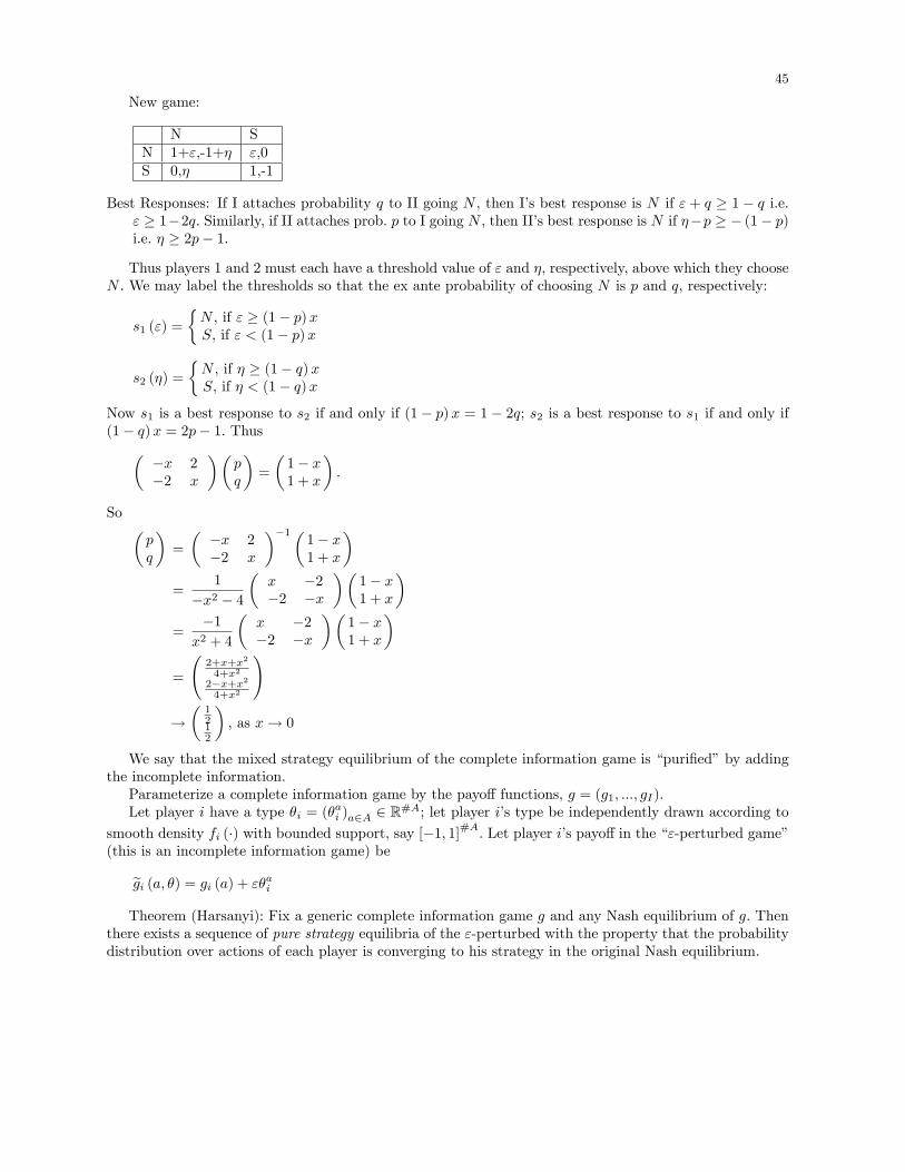
New game:
N SN 1+",-1+� ",0S 0,� 1,-1
Best Responses: If I attaches probability q to II going N , then I's best response is N if " + q � 1 � q i.e." � 1�2q. Similarly, if II attaches prob. p to I going N , then II's best response is N if ��p � � (1� p)i.e. � � 2p� 1.
Thus players 1 and 2 must each have a threshold value of " and �, respectively, above which they chooseN . We may label the thresholds so that the ex ante probability of choosing N is p and q, respectively:
s1 (") =
�N , if " � (1� p)xS, if " < (1� p)x
s2 (�) =
�N , if � � (1� q)xS, if � < (1� q)x
Now s1 is a best response to s2 if and only if (1� p)x = 1 � 2q; s2 is a best response to s1 if and only if(1� q)x = 2p� 1. Thus�
�x 2�2 x
��pq
�=
�1� x1 + x
�.
So �pq
�=
��x 2�2 x
��1�1� x1 + x
�=
1
�x2 � 4
�x �2�2 �x
��1� x1 + x
�=
�1x2 + 4
�x �2�2 �x
��1� x1 + x
�=
2+x+x2
4+x2
2�x+x24+x2
!
!�1212
�, as x! 0
We say that the mixed strategy equilibrium of the complete information game is \puri�ed" by addingthe incomplete information.Parameterize a complete information game by the payo� functions, g = (g1; :::; gI).Let player i have a type �i = (�
ai )a2A 2 R#A; let player i's type be independently drawn according to
smooth density fi (�) with bounded support, say [�1; 1]#A. Let player i's payo� in the \"-perturbed game"(this is an incomplete information game) be
egi (a; �) = gi (a) + "�aiTheorem (Harsanyi): Fix a generic complete information game g and any Nash equilibrium of g. Then
there exists a sequence of pure strategy equilibria of the "-perturbed with the property that the probabilitydistribution over actions of each player is converging to his strategy in the original Nash equilibrium.


Part IV
Dynamic Games of Incomplete Information


6. Sequential Rationality
See example 9.C.1 in MWG.
� Belief system � speci�es a probability distribution over nodes in each information set. Write � (zjh) forthe probability of node z given information set h.
� Strategy pro�le � is sequentially rational with respect to belief system � if each player's strategy maximizeshis expected utility at every information set, given the strategies of other players and the beliefs overnodes at that information set.
� Belief system � is consistent with strategy pro�le � if beliefs at each information set reached by � aregenerated by � and Bayes rule.
In MWG example 9.C.1, if belief system � is consistent with (In1;Accommodate) then we must have� (z1jh) = 1 and � (z2jh) = 0. On the other hand � (zjh) may take any value in [0; 1] and still be consistentwith (Out;Fight).
Observation: If � is a Nash equilibrium and � is consistent with �, then � is sequentially rational w.r.t. �at those information sets reached by �.
[Idea of Proof] Suppose not. Then there exists a player i, an information set h, and a strategy �0isuch that i's expected utility (under �) conditional on reaching info set h and following �0i exceeds thatof following �i. But now consider strategy �00i for player which equals �
0i at info set h and all info sets
following it and equals �i otherwise. Now ui (�00i ; ��i) > ui (�i; ��i), contradicting the assumption that �
is a Nash equilibrium.
Observation: Subgame perfection requires more sequential rationality than Nash equilibrium but fails todeal with MWG example 9.C.1.
De�nition: A strategy pro�le and beliefs system, (�; �), is a weak perfect Bayesian equilibrium if � issequentially rational with respect to � and � is consistent with �. Strategy pro�le � is a weak perfectBayesian equilibrium strategy pro�le if (�; �) is a weak perfect Bayesian equilibrium for some beliefsystem �.
[lecture 12]
Terminology: The terminology in this area is a nightmare. This de�nition follows MWG. Myerson callsthis a weak sequential equilibrium. This corresponds to requirements 1-3 in Gibbons. This is sometimesreferred to as perfect Bayesian equilibrium.
MWG example 9.C.1 has a unique perfect Bayesian equilibrium.In that case, the incumbent has a conditionally dominant strategies.In MWG example 9.C.3, weak PBE re�nes Nash equilibrium in a more subtle way.Two examples illustrate why we might want to put extra restrictions on out of equilibrium beliefs:
MWG example 9.C.4 illustrates how we would like to respect Bayes updating o� the equilibrium o� theequilibrium path; MWG example 9.C.5 shows that weak PBE fails to imply subgame perfection.The original approach to sequential rationality (due to Kreps and Wilson 1982) was the following. If
strategy pro�le �0 has \full support," all information sets are reached and thus there is a unique belief

50 6. Sequential Rationality
system �0 such that �0 is consistent with �0. Beliefs � are said to be fully consistent with � if there existsa full support sequence �k, with �k ! �, such that unique beliefs �k consistent with �k satisfy �k ! �.
De�nition: A strategy pro�le and beliefs system, (�; �), is a sequential equilibrium if � is sequentiallyrational w.r.t. � and � is fully consistent given �. Strategy pro�le � is sequential equilibrium strategypro�le if (�; �) is a sequential equilibrium for some belief system �.
It would be nice to try to capture directly some of the intuitive properties that fully consistent � mustsatisfy (without reference to perturbation sequence). This is approach of intermediate \perfect Bayesianequilibrium" [see, e.g., Gibbons requirement 4].
� If � is a sequential equilibrium strategy pro�le, then � is a subgame perfect Nash equilibrium.� All �nite period, �nite action games have at least one sequential equilibrium (and thus at least one weakperfect Bayesian equilibrium).
� See Myerson's Game Theory: Analysis of Con ict, chapter 4, for excellent discussion of sequential ratio-nality.
Lecture 1

Part V
Information Economics


6.1 Introduction 53
6.1 Introduction
Economics of information examines the role of information in economic relationship. It is therefore aninvestigation into the role of imperfect and incomplete information. In the presence of imperfect information,learning, Bayesian or not, becomes important, and in consequence dynamic models are prevalent. In thisclass we will focus mostly on incomplete or asymmetric information.The nature of information economics as a �eld is perhaps best understood when contrasted with the
standard general equilibrium theory. Information consists of a set of tools rather than a single methodology.Furthermore, the choice of tools is very issue driven. Frequently we will make use of the following tools:
� small number of participants� institutions may be represented by constraints� noncooperative (Bayesian) game theory� simple assumptions on bargaining: Principal-Agent paradigmWe refer to the Principal-Agent paradigm as a setting where one agent, called the Principal, can make all
the contract o�ers, and hence has (almost) all bargaining power and a second agent, called the Agent, canonly choose whether to accept or reject the o�er by the principal. With this general structure the interactivedecision problem can often by simpli�ed to a constrained optimization problem, where the Principal hasan objective function, and the Agent simply represents constraints on the Principal's objective function.Two recurrent constraints will be the participation constraint and the incentive constraint.The following scheme organizes most of the models prevalent in information economics according to
two criteria: (i) whether the informed or an uniformed agent has the initiative (makes the �rst move, o�ersthe initial contract, arrangement; and (ii) whether the uniformed agent is uncertain about the action orthe type (information) of the informed agent.
hidden action hidden informationinformed agent signalling
uninformed agent moral hazard adverse selection
The adverse selection model when extended to many agent will ultimately form the theoretical centerpieceof the lectures. In the later case we refer to it as the
many informed agents:mechanism design(social choice)
\mechanism design" problem which encompasses auctions, bilateral trade, public good provision, taxationand many other general asymmetric information problems. The general mechanism design problem can berepresented in a commuting diagram:
private information social choice(type) of agent i 2 I (allocation, outcome)
f�i 2 �igi2I �! f : � ! X �! x 2 X&
si : �i !Mi g :M ! X
& %fmi 2Migi2Imessages:from agentto principal
54
The upper part of the diagram represents the social choice problem, where the principal has to decide onthe allocation contingent on the types of the agent. The lower part represents the implementation problem,where the principals attempts to elicit the information by announcing an outcome function which mapsthe message (information) he receives from the privately informed agents into allocation. From the pointof view of the privately informed agents, this then represents a Bayesian game in which they can in uencethe outcome through their message.We shall start with two very simple, but classic models and results to demonstrate (i) how asymmetry of
information changes classical e�ciency results of markets and (ii) how asymmetry of information changesclassical arguments about the role of prices and the equilibrium process.
7. Akerlof's Lemon Model
7.1 Basic Model
This section is based on ?. Suppose an object with value v s U [0; 1] is o�ered by the seller. The valuationsare
us = �sv
and
ub = �bv
with �b > �s, and hence trading is always pareto-optimal. But trade has to be voluntary. We then ask isthere a price at which trade occurs. Suppose then at a price p trade would occur. What properties wouldthe price have to induce trade. The seller sells if
�sv � p
and thus by selling the object he signals that
v � p
�s(7.1)
The buyer buys the object if
�bE [v] � p (7.2)
and as he knows that (7.1) has to hold, he can form a conditional expectation, that
�bE [v jp ] � p, �bp
2�s� p (7.3)
Thus for the sale to occur,
�b � 2�s. (7.4)
Thus unless, the tastes di�er substantially, the market breaks down completely:
� market mechanism in which a lower prices increases sales fails to work as lowering the price decreasesthe average quality, lower price is \bad news".
� market may not disappear but display lower volume of transaction than socially optimal.
56 7. Akerlof's Lemon Model
7.2 Extensions
In class, we made some informed guesses how the volume of trade may depend on the distribution ofprivate information among the sellers. In particular, we ventured the claim that as the amount of privateinformation held by the sellers decreases, the possibilities for trade should increase. We made a secondobservation, namely that in the example we studied, for a given constellation of preferences by buyer andseller, represented by �b and �s, trade would either occur with positive probability for all prices or it wouldnot occur at all. We then argued that this result may be due to the speci�c density in the example, butmay not hold in general. We now address both issues with a uniform density with varying support andconstant mean:
v~U�1
2� "; 1
2+ "
�with " 2
�0; 12�. We can formalize the amount of private information by the variance of f (�) and how it
a�ects the e�ciency of the trade.We may redo the analysis above where the seller signals by selling the object at a �xed price p that
v � p
�s.
The buyer buys the object if
�bE [v jp ] � p,
The expected value is now given by
E [v jp ] =12 � "+
p�s
2
and hence for sale to occur
�b
12 � "+
p�s
2� p (7.5)
and inequality prevails if, provided that " 2 [0; 12 ) and 2�s > �b,
p � 1
2�b�s
1� 2"2�s � �b
Consider next the e�ciency issue. All types of sellers are willing to sell if
p = �s
�1
2+ "
�(7.6)
in which case the expected conditional value for the buyer is
1
2�b � �s
�1
2+ "
�or equivalently
�b � �s (1 + 2") (7.7)
Thus as the amount of private information, measured by ", decreases, the ine�ciencies in trade decrease.Notice that we derived a condition in terms of the preferences such that all sellers wish to sell. However

7.3 Wolinsky's Price Signal's Quality 57
even if condition (7.7) is not met, we can in general support some trade. This is indicated already in theinequality (7.5):
�b
12 � "+
p�s
2� p (7.8)
as the lhs increases slower in p, then the rhs of the inequality above. Thus there might be lower prices,which will not induce all sellers to show up at the market, yet allow some trade. We show how this can arisenext. For a positive mass of seller willing to sell the price may vary between p 2 (�s
�12 � "
�; �s�12 + "
�]. If
we then insert the price as a function of x 2 (�"; "], we �nd
�b
12 � "+
�s( 12+x)�s
2� �s
�1
2+ x
�or
�b1� "+ x
2� �s
�1
2+ x
�For a given �b; �s and ", we may then solve the (in-)quality for x, to �nd the (maximal) price p where thevolume of trade is maximized, or:
x =�b (1� ")� �s2�s � �b
:
Thus x is increasing in �b and decreasing in ";con�rming now in terms of the volume of trade our intuitionabout private information and e�ciency. In fact, we can verify that for a given " 2 [0; 12 ), the volume oftrade is positive, but as "! 1
2 becomes arbitrarily small and converges as expected to zero for �b < 2�s.
7.3 Wolinsky's Price Signal's Quality
This section is based on ?. Suppose a continuum of identical consumers. They have preferences
u = �v � p
and the monopolist can provide low and high quality: v = f0; 1g at cost 0 < c0 < c1. The monopolistselects price and quality simultaneously. Assume that � > c1 so that it is socially e�cient to produce thehigh quality good. Assume that the consumers do not observe quality before purchasing. It is clear that anequilibrium in which the monopolist sells and provides high quality cannot exist.Suppose now that some consumers are informed about the quality of the product, say a fraction �.
Observe �rst that if the informed consumers are buying then the uniformed consumer are buying as well.When is the seller better o� to sell to both segments of the market:
p� c1 � (1� �) (p� c0)
or
�p � c1 � (1� �) c0. (7.9)
We can then make two observations:
� high quality is supplied only if price is su�ciently high, \high price can signal high quality".� a higher fraction, �, of informed consumers favors e�ciency as it prevents the monopolist from cuttingquality
� the informational externality favors government intervention as individuals only take private bene�t andcost into account.

58 7. Akerlof's Lemon Model
7.4 Conclusion
We considered \hidden information" or \hidden action" models and suggested how asymmetry in informa-tion may reduce or end trade completely. In contrast to the canonical model of goods, which we may call\search goods", where we can assert the quality by inspection, we considered \experience goods" (?, ?),where the quality can only be ascertained after the purchase. The situation is only further acerbated with\credence goods" (?).In both models, there was room for a third party, government or other institution, to induce pareto
improvement. In either case, and improvement in the symmetry of information lead to an improvementin the e�ciency of the resulting allocation. This suggest that we may look for optimal or equilibriumarrangements to reduce the asymmetry in information, either through:
� costly signalling� optimal contracting to avoid moral hazard, or� optimal information extraction through a menu of contract (i.e. mechanism design).
7.5 Reading
The lecture is based on Chapter 1 in ?, Chapter 2 in ?, and Chapter 5 in ?.
[Lecture 2]
8. Job Market Signalling
Consider the following game �rst analyzed by ?. Nature chooses a workers type (productivity) a 2 f1; 2g.The worker has productivity a with probability p (a). For notational convenience, we de�ne
p , p (a = 2) :
The worker can choose an educational level e 2 R+. There are a two �rms who compete in wages w1; w2.The worker chooses the �rm The workers utility is
u (w; e; a) = w � e
a.
The objective function of the �rm is given by
minX
a2f1;2g
(a� w)2 p (a je )
We observe that
@2u (w; e; a)
@e@a=1
a2> 0
and thus type and strategic variable are complements (supermodular).
8.1 Pure Strategy
A pure strategy for the worker is a function
be : f1; 2g ! R+
A pure strategy for the �rm is a function
w : R+ ! R+
where w (e) is the wage o�ered to a worker of educational level e.
8.2 Perfect Bayesian Equilibrium
The novelty in signalling games is that the uninformed party gets a chance to update its prior belief onthe basis of a signal sent by the informed party. The updated prior belief is the posterior belief, dependingon e and denoted by p (a je ). The posterior belief is a mapping
p : R+ ! [0; 1]
60 8. Job Market Signalling
In sequential or extensive form games we required that the strategy are sequential rational, or time consis-tent. We now impose a similar consistency requirement on the posterior beliefs by imposing the Bayes' rulewhenever possible. Since p (a je ) is posterior belief, and hence a probability function, it is required that:
8e; 9p (a je ) ; s.th. p (a je ) � 0; andX
�2f1;2g
p (a je ) = 1: (8.1)
Moreover, when the �rm can apply Bayes law, it does so, or
if 9a s.th. at e� (a) = e; then p (a je ) = p (a)Pfa0je�(a)=eg p (a
0): (8.2)
We refer to educational choice which are selected by some worker-types in equilibrium, or if 9a s.th. ate� (a) = e, as \on-the-equilibrium path" and educational choices s.th. @a with e� (a) = e as \o�-the-equilibrium-path".As before it will be sometimes easier to refer to
p (e) , p (a = 2 je )
and hence
p (1 je ) = 1� p (e) :
De�nition 8.2.1 (PBE). A pure strategy Perfect Bayesian Equilibrium is a set of strategies fe� (a) ; w� (e)gand posterior beliefs p (e) such that:
1. 8e; 9p� (a je ) ; s.th. p� (a je ) � 0; andP
�2f1;2g p� (a je ) = 1;
2. 8i; w�i (e) =P
a p� (a je ) a;
3. 8a; e� (a) 2 argmax�w� (e)� e
a
4. if 9a s.th. at e� (a) = e; then:
p (a je ) = p (a)Pfa0je�(a)=eg p (a
0):
[To Be Added: Notions of On and Off the Equilibrium Path]
De�nition 8.2.2 (Separating PBE). A pure strategy PBE is a separating equilibrium if
a 6= a0 ) e (a) 6= e (a0) .
De�nition 8.2.3 (Pooling PBE). A pure strategy PBE is a pooling equilibrium if
8a; a0 ) e (a) = e (a0) .
[Lecture 3]
Theorem 8.2.1.
1. A pooling equilibrium exists for all education levels e = e (1) = e (2) 2 [0; p] :2. A separating equilibrium exists for all e (1) = 0 and e (2) 2 [1; 2].

8.2 Perfect Bayesian Equilibrium 61
Proof. (1) We �rst construct a pooling equilibrium. For a pooling equilibrium to exist it must satisfy thefollowing incentive compatibility constraints
8e; 1 + p (e�)� e� � 1 + p (e)� e (8.3)
and
8e; 1 + p (e�)� e�
2� 1 + p (e)� e
2(8.4)
Consider �rst downward deviations, i.e. e < e�, then (8.3) requires that
p (e�)� p (e) � e� � e: (8.5)
Then consider upward deviations, i.e. e > e�, then (8.4) requires that
p (e)� p (e�) � 1
2(e� e�) : (8.6)
We can then ask for what levels can both inequalities be satis�ed. Clearly both inequalities are easiest tosatisfy if
e < e� ) p (e) = 0
e > e� ) p (e) = 0;
which leaves us with
e < e� ) p � e� � e (8.7)
e > e� ) �p � 1
2(e� e�) :
We may then rewrite the inequalities in (8.7) as
e < e� ) e� � p+ e (8.8)
e > e� ) e� � p+ 2e
As the inequality has to hold for all e, the asserting that 0 � p � e� holds, follows immediately.(2) Consider then a separating equilibrium. It must satisfy the following incentive compatibility con-
straints
8e; 1 + p (e�1)� e�1 � 1 + p (e)� e
and
8e; 1 + p (e�2)�e�22� 1 + p (e)� e
2: (8.9)
As along the equilibrium path, the �rms must apply Bayes law, we can rewrite the equations as
8e; 1� e�1 � 1 + p (e)� e
and
8e; 2� e�2
2� 1 + p (e)� e
2:
Consider �rst the low productivity type. It must be that e�1 = 0. This leaves us with
p (e) � e: (8.10)
62 8. Job Market Signalling
But if e = e�2 is supposed to be part of a separating equilibrium, then p (e�2) = 1. Thus it follows further
from (8.10) that e�2 � 1, for otherwise we would not satisfy 1 = p (e�2) � e�2. Finally, we want to determinean upper bound for e�2. AS we cannot require the high ability worker to produce too much e�ort otherwisehe would mimic the lower ability, we can rewrite (8.9) to obtain:
1� p (e) � 1
2(e�2 � e) ;
which is easiest to satisfy if
p (e) = 0;
and hence
8e; 2 + e � e�2which implies that:
e�2 � 2.
which completes the proof.
The theorem above only de�nes the range of educational choices which can be supported as an equi-librium but is not a complete equilibrium description as we have not speci�ed the beliefs in detail. Thejob market signalling model suggests a series of further questions and issues. There were mutliple equil-bria, reducing the predictive ability of the model and we may look at di�erent approaches to reduced themultiplicitly:
� re�ned equilibrium notion� di�erent model: informed principal
The signal was modelled as a costly action. We may then ask for conditions:
� when do costly signals matter for Pareto improvements (or simply separation): Spence-Mirrlees singlecrossing conditions
� when do costless signals matter: cheap-talk games.
In the model, education could also be interpreted as an act of disclosure of information through theveri�cation of the private information by a third party. It may therefore be of some interest to analyze thepossibilities of voluntary information disclosure.
8.3 Equilibrium Domination
The construction of some of the equilibria relied on rather arbitrary assumptions about the beliefs of the�rms for educational choice levels o� the equilibrium path. Next we re�ne our argument to obtain somelogical restrictions on the beliefs. The restrictions will not be bases on Bayes law, but on the plausibilityof deviations as strategic choices by the agents. The notions to be de�ned follow ?.
De�nition 8.3.1 (Equilibrium Domination). Given a PBE, the message e is equilibrium-dominatedfor type a, if for all possible assessments p (a je ) (or simply p(e)):
w� (e� (a))� e� (a)
a> w (e)� e
a
or equivalently
1 + p� (e� (a))� e� (a)
a> 1 + p (e)� e
a

8.3 Equilibrium Domination 63
De�nition 8.3.2 (Intuitive Criterion). If the information set following e is o� the equilibrium pathand e is equilibrium dominated for type a, then
p (a je ) = 0: (8.11)
De�nition 8.3.3. A PBE where all beliefs o� the equilibrium path satisfy the intuitive criterion is said tosatisfy the intuitive criterion.
Theorem 8.3.1 (Uniqueness). The unique Perfect Bayesian equilibrium outcome which satis�es theintuitive criterion is given by
fe�1 = 0; e�2 = 1; w� (0) = 1; w� (1) = 2g : (8.12)
The beliefs are required to satisfy
p� (e) =
8<: 0; for e = 02 [0; e] ; for 0 < e < 11; for e � 1
Remark 8.3.1. The equilibrium outcome is referred to as the least-cost separating equilibrium (or ? equi-librium)
Proof. We �rst show that there can't be any pooling equilibria satisfying the intuitive criterion, and thenproceed to show that only one of the separating equilibria survives the test of the intuitive criterion.Suppose 0 � e� � p. Consider e 2 (e� + (1� p) ; e� + 2 (1� p)). Any message e in the interval is
equilibrium dominated for the low productivity worker as
1 + p� e� > 2� e;
but any message in the interval is not equilibrium dominated for the high productivity worker, as
1 + p� e
2
�< 2� e
2
and thus for e = e� + (1� p), we have
p < 1� (1� p)2
, 1
2p <
1
2;
which certainly holds. Thus if (e; p (e)) satis�es the intuitive criterion, we must have p (e) = 1 for e 2(e� + (1� p) ; e� + 2 (1� p)), but then pooling is not an equilibrium anymore as the high productivityworker has a pro�table deviation with any e 2 (e� + (1� p) ; e� + 2 (1� p)).Consider now the separating equilibria. For e�2 > 1, any e 2 (1; e�2) is equilibrium dominated for the low
ability worker as
1 > 2� e;
but is not equilibrium dominated for the high ability worker, as
2� e�2
2< 2� e
2.
It follows that p (e) = 1 for all e 2 (1; e�2). But then e�2 > 1, cannot be supported as an equilibrium as thehigh ability worker has a pro�table deviation by lowering his educational level to some e 2 (1; e�2), and stillreceive his full productivity in terms of wages. It remains e�2 = 1 as the unique PBE satisfying the intuitivecriterion.
Criticism. Suppose p! 1:
[Lecture 4]
64 8. Job Market Signalling
8.4 Informed Principal
As plausible as the Cho-Kreps intuitive criterion may be, it does seem to predict implausible equilibriumoutcomes in some situations. For example, suppose that, p, the prior probablity that a worker of typea = 2 is present, is arbitrarily large, (p �! 1). In that case, it seems a rather high cost to pay to incur aneducation cost of
c(e = 1) =1
2
just to be able to raise the wage by a commensurately small amount �w = 2 � (1 + p) �! 0 as p ! 1.Indeed, in that case the pooling equilibrium where no education costs are incurred seems a more plausibleoutcome. This particular case should serve as a useful warning not to rely too blindly on selection criteria(such as Cho-Kreps' intuitive criterion) to single out particular PBEs.
8.4.1 Maskin and Tirole's informed principal problem
Interestingly, much of the problem of multiplicity of PBEs disappears when the timing of the game ischanged to letting agent and principal sign a contract before the choice of signal. This is one importantlesson to be drawn from ?.To see this, consider the model of education as speci�ed above and invert the stages of contracting
and education choice. That is, now the worker signs a contract with his/her employer before undertakingeducation. This contract then speci�es a wage schedule contingent on the level of education chosen by theworker after signing the contract.Let fw(e)g denote the contingent wage schedule speci�ed by the contract.Consider the problem for the high productivity worker. Suppose he would like to make an o�er by
which he can separate himself from a low ability worker
maxfe;w(e)g
nw (e)� e
2
osubject to
w (e1)� e1 � w (e2)� e2 (IC1)
and
w (e2)�e22� w (e1)�
e12
(IC2)
and
a1 � w (e1) � 0 (IR1)
a2 � w (e2) � 0 (IR2)
Thus to make incentive compatibility as easy as possible he suggests e1 = 0 and w (e1 = 0) = 1. Asw (e2) = 2, it follows that after setting e2 = 1, he indeed maximizes his payo�.Suppose instead he would like to o�er a pooling contract. Then he would suggest
maxe;w
nw � e
2
o1 + p� w � 0 (IR1)
which would yield w = 1 + p for all e.This suggest that there are two di�erent cases to consider:

8.5 Spence-Mirrlees Single Crossing Condition 65
1. 1 + p � 2� 12 : a high productivity worker is better o� in the \least cost" separating equilibrium than
in the e�cient pooling equilibrium.2. 1 + p > 2� 1
2 : a high productivity worker is better o� in the e�cient pooling equilibrium.
It is easy to verify that in the case where p � 12 , the high productivity worker cannot do better than
o�ering the separating contract, nor can the low productivity worker. More precisely, the high productivityworker strictly prefers this contract over any contract resulting in pooling or any contract with more costlyseparation. As for the low productivity worker, he has everything to lose by o�ering another contract whichwould identify himself.In the alternative case where p > 1
2 , the unique equilibrium contract is the one where:
w�(e) = 1 + p for all e � 0.
Again, if the �rm accepts this contract, both types of workers choose an education level of zero. Thus, onaverage the �rm breaks even by accepting this contract, provided that it is as (or more) likely to originatefrom a high productivity worker than a low productivity worker. Now, a high productivity worker strictlyprefers to o�er this contract over any other separating contract. Similarly, a low productivity worker haseverything to lose from o�ering another contract and thus identifying himself. Thus, in this case again thisis the unique contract o�er made by the workers.
8.5 Spence-Mirrlees Single Crossing Condition
8.5.1 Separating Condition
Consider now a general model with a continuum of types:
A � R+
and an arbitrary number of signals
E � R+
with a general quasilinear utility function
u (t; e; a) = t+ v (e; a)
where we recall that the utility function used in Spence model was given by:
u (t; e; a) = t� e
a
We now want ask when is it possible in general to sustain a separating equilibrium for all n agents, suchthat
a 6= a0 ) e 6= e0
Suppose we can support a separating equilibrium for all types, then we must be able to satisfy for a0 > aand without loss of generality e0 > e:
t+ v (e; a) � t0 + v (e0; a), t� t0 � v (e0; a)� v (e; a) (8.18)
and
66 8. Job Market Signalling
t0 + v (e0; a0) � t+ v (e; a0), t� t0 � v (e0; a0)� v (e; a0) ; (8.19)
where t , t (e) and t0 , t (e0), and by combining the two inequalities, we �nd
v (e0; a)� v (e; a) � v (e0; a0)� v (e; a0) ; (8.20)
or similarly, again recall that e < e0
v (e; a0)� v (e; a) � v (e0; a0)� v (e0; a) : (8.21)
We then would like to know what are su�cient conditions on v (�; �) such that for every a there exists esuch that (8.20) can hold.
8.6 Supermodular
De�nition 8.6.1. A function v : E � A ! R has increasing di�erences in (e; a) if for any a0 > a,v(e; a0)� v(e; a) is nondecreasing in e.
Note that if v has increasing di�erences in (e; a), it has increasing di�erences in (a; e). Alternatively,we say the function v is supermodular in (e; a).If v is su�ciently smooth, then v is supermodular in (e; a) if and only if @2v=@e@a � 0.As the transfers t; t0 could either be determined exogeneously, as in the Spence signalling model through
market clearing conditions, or endogeneously, as in optimally chosen by the mechanism designer, we want toask when we can make a separation incentive compatible. We shall not consider here additional constraintssuch as a participation constraints. We shall merely assume that t (a), i.e. the transfer that the agent of typea gets, t (a), conditional on the sorting allocation fa; e (a) ; t (a)g to be incentive compatible, is continuouslydi�erentiable and strictly increasing.
Theorem 8.6.1. A necessary and su�cient condition for sorting ((8.18) and (8.19)) to be incentive com-patible for all t (a) is that
1. v (e; a) is strictly supermodular2. @v
@e < 0 everywhere
Proof. We shall also suppose that v (�; �) is twice continously di�erentiably. The utility function of the agentis given by
t (a) + v (e (a) ; a) ,
where a is the true type of agent a and e (a) is the signal the informed agent sends to make the uninformedagent believe he is of type a.(Su�ciency) For e (a) to be incentive compatible, a must locally solve for the �rst order conditions of theagent at a = a, namely the true type:
t0 (a) +@v (e (a) ; a)
@e
de
da= 0, at a = a (8.22)
But Fix the payments t (a) as a function of the type a to be t (a) and suppose without loss of generalitythat t (a) is continuously di�erentiable. The equality (8.22) de�nes a di�erential equation for the separatinge�ort level
de
da=
t0 (a)@v(e(a);a)
@e
(8.23)

8.7 Supermodular and Single Crossing 67
for which a unique solution exists given a initial condition, say t (0) = 0. The essential element is that the�rst order conditions is only an optimal condition for agent with type a and nobody else, but this followsfrom strict supermodularity. As
t0 (a)
and
de
da
are independent of the true type, a, it follows that if
@2v (e; a)
@e@a> 0,
for all e and a, then (8.22) can only identify truthtelling for agent a.(Necessity) For any particular transfer policy t (a), we may not need to impose the supermodularity con-dition everywhere, and it might often by su�cient to only impose it locally, where it is however necessaryto guarantee local truthtelling, i.e.
@v (e (a) ; a)
@e@a> 0
at e = e (a). However, as we are required to consider all possible transfers t (a) with arbitrary positive slopes,we can guarantee that for every a and every e there is some transfer problem t (a) such that e (a) = e by(8.23), and hence under the global condition on t (a), supermodularity becomes also a necessary conditionfor sorting.
8.7 Supermodular and Single Crossing
In the discussion above we restricted our attention to quasilinear utility function. We can generalize all thenotions to more general utility functions. We follow the notation in ?. Let
U (x; y; t) : R3 ! R
where x is in general the signal (or allocation), y an additional instrument, such as money transfer and tis the type of the agent.
De�nition 8.7.1 (Spence-Mirrlees). The function U is said to satisfy the (strict) Spence-Mirrlees con-dition if
1. the ratio
UxjUyj
is (increasing) nondecreasing in t, and Uy 6= 0, and2. the ratio has the same sign for every (x; y; t).
De�nition 8.7.2 (Single-Crossing). The function U is said to satisfy the single crossing property in(x; y; t) if for all (x0; y0) � (x; y)1. whenever U (x0; y0; t) � U (x; y; t), then U (x0; y0; t0) � U (x; y; t0) for all t0 > t;2. whenever U (x0; y0; t) > U (x; y; t), then U (x0; y0; t0) > U (x; y; t0) for all t0 > t;
? show that the notions of single crossing and the Spence Mirrlees conditions are equivalent.Thus the supermodularity condition is also often referred to as the single-crossing or Spence-Mirrlees
condition, where Mirrlees used the di�erential form for the �rst time in ?. The notions of supermodu-larity and single-crossing are exactly formulated in ? and for some corrections ? Some applications tosupermodular games are considered by ? and ?. The mathematical theory is, inter alia, due to ? and ?.
68 8. Job Market Signalling
8.8 Signalling versus Disclosure
Disclosure as private but certi�able information. Signalling refered to situations where private informationis neither observable nor veri�able. That is to say, we have considered private information about suchthings as individual preferences, tastes, ideas, intentions, quality of projects, e�ort costs, etc, which cannotreally be measured objectively by a third party. But there are other forms of private information, such asan individual's health, the servicing and accident history of a car, potential and actual liabilities of a �rm,earned income, etc, that can be certi�ed or authenticated once disclosed. For these types of informationthe main problem is to get the party who has the information to disclose it. This is a simpler problemthan the one we have considered so far, since the informed party cannot report false information. It canonly choose not to report some piece of information it has available. The main results and ideas of thisliterature is based on ? and ?.
8.9 Reading
The material of this lecture is covered by Section 4 of ? and for more detail on the Spence-Mirrleesconditions, see ?.
9. Moral Hazard
Today we are discussing the optimal contractual arrangement in a moral hazard setting
9.1 Introduction and Basics
In contractual arrangements in which the principal o�ers the contract, we distinguish between
hidden information - `adverse selection'
and
hidden action - `moral hazard'
The main trade-o� in adverse selction is between e�cient allocation and informational rent. In moralhazard settings it is between risk sharing and wok incentives. Today we are going to discuss the basic moralhazard setting. As the principal tries to infer from the output of the agent about the e�ort choice, theprincipal engages in statistical inference probelms. Today we are going to develop basic insights into theoptimal contract and use this is an occasion to introduce three important informational notions:
1. monotone likelihood ratio2. garbling in the sense of Blackwell3. su�cient statistic
The basic model goes as follows. An agent takes action that a�ect utility of principal and agent.Principalobserves \outcome" x and possible some \signal" s but not \action" a of agent. Agent action in absenceof contract is no e�ort. In uence agents action by o�ering transfer contingent on outcome.
Example 9.1.1. Employee employer e�ect (non observable), Property insurance (�re, theft)
FB: agents action is observable (risk sharing)SB: agents action is unobservable (risk sharing-incentive)
9.2 Binary Example
The agent can take action a 2 fal; ahg at cost c 2 fcl; chg. The outcomes x 2 fxl; xhg occur randomly,where the probabilities are governed by the action as follows.
pl = Pr (xh jal ) < ph = Pr (xh jah )The principal can o�er a wage, contingent on the outcome w 2 fwl; whg to the agent and the utility of theagent is
u (wi)� ciand of the principal it is
v (xi � wi)where we assume that u and v are strictly increasing and weakly concave.
70 9. Moral Hazard
9.2.1 First Best
We consider initially the optimal allocation of risk between the agents in the presence of the risk and withobservable actions. If the actions are observable, then the principal can induce the agent to choose thepreferred action a� by
w (xi; a) = �1
if a 6= a� for all xi. As the outcome is random and the agents have risk-averse preference, the optimalallocation will involve some risk sharing. The optimal solution is characterized by
maxfwl;whg
fpiv (xh � wh) + (1� pi) v (xl � wl)g
subject to
piu (wh) + (1� pi)u (wl)� ci � U; (�)
which is the individual rational constraint. Here we de�ne
w (xi; a�) , wi
This is a constrained optimization problem, and the �rst order conditions from the Lagrangian
L (wl; wh; �) = piv (xh � wh) + (1� pi) v (xl � wl) + � (piu (wh) + (1� pi)u (wl)� ci)
are given by
V 0 (xi � wi)U 0 (wi)
= �;
which is Borch's rule.
9.2.2 Second Best
Consider now the case in which the action is unobservable and therefore
w (xi; a) = w (xi)
for all a. Suppose the principal wants to induce high e�ort, then the incentive constraint is:
phu (wh) + (1� ph)u (wl)� ch � plu (wh) + (1� pl)u (wl)� cl
or
(ph � pl) (u (wh)� u (wl)) � ch � cl (9.1)
as pl ! ph wh�wl must increase, incentives become more high-powered. Tthe principal also has to respecta participation constraint (or individual rationality constraint)
phu (wh) + (1� ph)u (wl)� ch � �U (9.2)
We �rst show that both constraints will be binding if the principal maximizes
maxfwh;wlg
ph (xh � wh) + (1� ph) (xl � wl)
9.3 General Model with �nite outcomes and actions 71
subject to (9.1) and (9.2). For the participation constraint, principal could lower both payments and bebetter o�. For the incentive constraint, subtract
(1� ph) "u0 (wh)
from wh and add
ph"
u0 (wl)
to wl. Then the incentive constraint would still hold for " su�ciently small. Consider then participationconstraint. We would substract utility
(1� ph) "
from u (wh) and add
ph"
to u (wl), so that the expected utility remains constant. But the wage bill would be reduced for the principalby
"ph (1� ph)�
1
u0 (wh)� 1
u0 (wl)
�> 0;
since wh > wl by concavity. The solution is :
u (wl) = U �chpl � phclph � pl
and
u (wh) = U �chpl � phclph � pl
+ch � clph � pl
9.3 General Model with �nite outcomes and actions
Suppose
xi 2 fx1; :::; xIg
and
aj 2 fa1; :::aJg
and the probability
pij = Pr (xi jaj )
the utility is u (w)� a for agent and x� w for the principal.
72 9. Moral Hazard
9.3.1 Optimal Contract
The pricnipals problem is then
maxfwigIi=1;j
(IXi=1
(xi � wi) pij
)
given the wage bill the agent selects aj if and only if
IXi=1
u (wi) pij � aj �IXi=1
u (wi) pik � ak (�k)
and
IXi=1
u (wi) pij � aj � U (�)
Fix aj , then the Lagrangian is
L (wij ; �; �) =(
IXi=1
(xi � wi) pij
)+Xk 6=j
(IXi=1
u (wi) (pij � pik)� (aj � ak))
+�
(IXi=1
u (wi) pij � aj
)Di�erentiating with respect to wij yields
1
u0 (wi)= �+
Xk 6=j
�k
�1� pik
pij
�; 8i (9.3)
With a risk-avers principal the condition (9.3) would simply by modi�ed to:
v0 (xi � wi)u0 (wi)
= �+Xk 6=j
�k
�1� pik
pij
�; 8i (9.4)
In the absence of an incentive problem, or �k = 0, (9.4) states the Borch rule of optimal risk sharing:
v0 (xi � wi)u0 (wi)
= �; 8i.
which states that the ratio of marginal utilities is equalized across all states i.We now ask for su�cient conditions so that higher outcomes are rewarded with higher wages. As wi
increases as the right side increases, we might ask for conditions when the rhs is increasing in i. To dothis we may distinguish between the `downward' binding constraints (�k; k < j) and the `upward' bindingconstraints (�k; k > j). Suppose �rst then that there were only `downward' binding constraints, i.e. eitherj = J , or �k = 0 for k > j. Then a su�cient for monotonicity in i would clearly be that
pikpij
is decreasing in i for all k < j.
9.3 General Model with �nite outcomes and actions 73
9.3.2 Monotone Likelihood Ratio
The ratio
pikpij
are called likelihood ratio. We shall assume a monotone likelihood ratio condition, or 8i < i0;8k < j :pikpij
>pi0kpi0j
or reversing the ratio
pijpik
<pi0jpi0k
so that the likelihood ratio increases with the outcome. In words, for a higher outcome xi0 , it becomes morelikely, the action pro�le was high (j) rather than low (k). By modifying the ratio to:
pi0kpik
<pi0jpij
we get yet a di�erent interpretation. An increase in the action increases the relative probability of a highoutcome versus a low outcome.The appearance of the likelihood ratio can be interpreted as the question of estimating a `parameter' a
from the observation of the `sample' xi as the following two statements are equivalent:
aj is the maximum likelhood estimator of a given xi , 8k; pikpij � 1.
As is explained in Hart-Holmstr�om [1986]:
The agent is punished for outcomes that revise belief about aj down, while he is rewarded for out-comes that revise beliefs up. The agency problem is not an inference problem in a strict statisticalsense; conceptually, the principal is not inferring anything about the agent's action from x becausehe already knows what action is being implemented. Yet, the optimal sharing rule re ects preciselythe pricing of inference.
�1� pik
pij
�> 0 if pik < pij�
1� pikpij
�< 0 if pik > pij
The monoticity in the optimal contract is then established if we can show that the downward bindingconstraints receive more weight than the upward binding constraints. In fact, we next give conditions whichwill guarantee that �k = 0 for all k > j.
9.3.3 Convexity
The cumulative distribution function of the outcome is convex in a: for aj < ak < al and � 2 [0; 1] suchthat for
ak = �aj + (1� �) al
we have

74 9. Moral Hazard
Pik � �Pij + (1� �)Pil
The convexity condition then states that the return from action are stochastically decreasing. Next weshow in two steps that monotone likelihood and convexity are su�cient to establish monotonicity. Theargument is in two steps and let aj be the optimal action.First, we know that for some j < k, �j > 0. Suppose not, then the optimal choice of ak would be same
if we were to consider A or fak; :::; aJg. But relative to fak; :::; aJg we know that ak is the least cost actionwhich can be implemented with a constant wage schedule. But extending the argument to A, we know thata constant wage schedule can only support the least cost action a1.Second, consider fa1; :::; akg. Then ak is the most costliest action and by MLRP wi is increasing in i.
We show that ak remains the optimal choice for the agent when we extend his action to A. The proof isagain by contradiction. Suppose there is l > k s.th.
IXi=1
u (wi) pik � ak <IXi=1
u (wi) pil � al:
and let j < k be an action where �k > 0 and hence
IXi=1
u (wi) pik � ak =IXi=1
u (wi) pij � aj :
Then there exists � 2 [0; 1] such that
ak = �aj + (1� �) al
and we can apply convexity, by �rst rewriting pik and using the cumulative distribution function
IXi=1
u (wi) pik � ak =IXi=1
(u (wi)� u (wi+1))Pik + u (wI)� ak
By rewriting the expected value also for aj < ak < al, we obtain
IXi=1
(u (wi)� u (wi+1))Pik + u (wI)� ak �
�
IXi=1
(u (wi)� u (wi+1))Pij + u (wI)� aj
!
+(1� �)
IXi=1
(u (wi)� u (wi+1))Pil + u (wI)� al
!The later is of course equivalent to
�
IXi=1
u (wi) pij � aj
!+ (1� �)
IXi=1
u (wi) pil � al
!The inequality follows from the convexity and the fact that we could assume wi to be monotone, so thatu (wi)� u (wi+1) � 0.A �nal comment on the monotonicity of the transfer function : Perhaps a good reason why the function
wi must be monotonic is that the agent may be able to arti�cially reduce performance. In the aboveexample, he would then arti�cially lower it from xj to xi whenever the outcome is xj .

9.4 Information and Contract 75
9.4 Information and Contract
9.4.1 Informativeness
We now ask how does the informativeness of a signal structure a�ect the payo� of the agent. Consider astochastic matrix Q which modi�es the probabilities pij such that
pkj =IXi=1
qkipij ; (9.5)
such that qki � 0 and
KXk=1
qki = 1
for all i. The matrix is called stochastic as all its entries are nonnegative and every column adds up toone. Condition (9.5) is a generalization of the following idea. Consider the information structure given bypij . Each time the signal xi is observed, it is garbled by a stochastic mechanism that is independent of theaction aj , which may be interpreted here as a state. It is transformed into a vector of signals bxk. The termqki can be interpreted as a conditional probability of bxk given xi. Clearly pkj are also probabilities.Suppose the outcomes undergo a similar transformation so that
KXk=1
xkpkj =IXi=1
xipij ;
for all j. Thus the expected surplus stays the same for every action. It can be achieved (in matrix language)by assuming that x = Q�1x.In statistical terms, inferences drawn on aj after observing bx with probabilities bp will be less precise
than the information drawn from observing x with probability p.Consider now in the (p; x) model a wage schedule bwi which implements aj . Then we �nd a new wage
schedule for the (p; x) problem based on bw such that aj is also implementable in (p; x) problem, yet wewill see that it involves less risk imposed on the agent and hence is better for the principal. Let
u (wi) =
KXk=1
qkiu ( bwk) (9.6)
We can then write
IXi=1
piju (wi) =IXi=1
pij
KXk=1
qkiu ( bwk)!
=KXk=1
pkju ( bwk)But the implementation in (p; x) is less costly for the principal than the one in (p; x) which proves theresult. But (9.6) immediately indicates that it is less costly for the principal as the agent has a concaveutility function. This shows in particular that the optimal contract is only a second best solution as the�rst best contains no additional noise.
76 9. Moral Hazard
9.4.2 Additional Signals
Suppose besides the outcome, the principal can observe some other signal, say y 2 Y = fy1; ::::; yl; :::; yLg,which could inform him about the performance of the agent. The form of the optimal contract can thenbe veri�ed to be
1
u0�wli� = �+X
k 6=j�k
1� p
lik
plij
!.
Thus the contract should integrate the additional signal y if there exists some xi and yl such that for ajand ak
plikplij
6= pl0
ik
pl0ij
;
but the inequality simply says that
x
is not a su�cient statistic for (x; y) as it would be if we could write the conditional probability as follows
f (xi; yl jaj ) = h (xi; yl) g (xi jaj ) :
Thus, Hart-Holmstr�om [1986] write:
The additional signal s will necessarily enter an optimal contract if and only if it a�ects theposterior assessment of what the agent did; or perhaps more accurately if and only if s in uencesthe likelihood ratio.
9.5 Linear contracts with normally distributed performance and exponentialutility
This constitutes another \natural" simple case. Performance is assumed to satisfy x = a + ", where " isnormally distributed with zero mean and variance �2. The principal is assumed to be risk neutral, whilethe agent has a utility function :
U(w; a) = �e�r(w�c(a))
where r is the (constant) degree of absolute risk aversion (r = �U 00=U 0), and c(a) = 12ca
2:We restrict attention to linear contracts:
w = �x+ �:
A principal trying to maximize his expected payo� will solve :
maxa;�;�
E(x� w)
subject to :
9.5 Linear contracts with normally distributed performance and exponential utility 77
E(�e�r(w�c(a))) � U(w)
and
a 2 argmaxa
E(�e�r(w�c(a)))
where U(w) is the default utility level of the agent, and w is thus its certain monetary equivalent.
9.5.1 Certainty Equivalent
The certainty equivalent w of random variable x is de�ned as follows
u (w) = E [u (x)]
The certainy equivalent of a normally distributed random variable x under CARA preferences, hence wwhich solves
�e�rw = E��e�rx
�has a particularly simple form, namely
w = E [x]� 12r�2 (9.7)
The di�erence between the mean of random variable and its certain equivalent is referred to as the riskpremium:
1
2r�2 = E [x]� w
9.5.2 Rewriting Incentive and Participation Constraints
Maximizing expected utility with respect to a is equivalent to maximizing the certainty equivalent wealthbw(a) with respect to a, where bw(a) is de�ned by�e�r bw(a) = E(�e�r(w�c(a)))
Hence, the optimization problem of the agent is equivalent to:
a 2 argmax f bw(a)g =2 argmax
��a+ � � 1
2ca2 � r
2�2�2
�which yields
a� =�
c
Inserting a� into the participation constraint
��
c+ � � 1
2c��c
�2� r
2�2�2 = �w
78 9. Moral Hazard
yields an expression for �,
� = �w +r
2�2�2 � 1
2
�2
c
This gives us the agent's e�ort for any performance incentive �. The principal then solves :
max�
��
c� ( �w + r
2�2�2 +
1
2
�2
c)
�The �rst order conditions are
1
c� (r��2 + �
c) = 0;
which yields :
�� =1
1 + rc�2
E�ort and the variable compensation somponent thus go down when c (cost of e�ort); r (degree of risk aver-sion), and �2 (randomness of performance) go up, which is intuitive. The constant part of the compensationwill eventually decrease as well as r; c or �2 become large, as
� = �w +
1
2
r�2 � 1c
(1 + rc�2)2
!:
9.6 Readings
The following are classic papers in the literature on moral hazard: ?, ?, ?, ?, ?, ?,?,?.
[Lecture 7]

Part VI
Mechanism Design

10. Introduction
Mechanism design. In this lecture and for the remainder of this term we will look at a special class ofgames of incomplete information, namely games of mechanism design. Examples of these games include: (i)monopolistic price discrimination, (ii) optimal taxation, (iii) the design of auctions, and (iv) the provisionof public goods.Information extraction, truthtelling, and incentives.All these examples have in common there is
a \principal" (social planner, monopolist, etc.) who would like to condition her action on some informationthat is privately known by the other players, called \agents". The principal could simply ask the agentsfor their information, but they will not report truthfully unless the principal gives them an incentive to doso, either by monetary payments or with some other instruments that she controls. Since providing theseincentives is costly, the principal faces a trade-o� that often results in an e�cient allocation.Principal's objective. The distinguishing characteristic of the mechanism design approach is that
the principal is assumed to choose the mechanism that maximizes her expected utility, as opposed to usinga particular mechanism for historical or institutional reasons. (Caveat: Since the objective function of theprincipal could just be the social welfare of the agents, the range of problem which can be studies is ratherlarge.)Single agent. Many applications of mechanism design consider games with a single agent (or equivalent
with a continuum of in�nitesimal small agents). For example, in a second degree price discrimination bya monopolist, the monopolist has incomplete information about the consumer's willingness to pay for thegood. By o�ering a price quantity schedules he attempts to extract the surplus from the buyer.Many agents. Mechanism design can also be applied to games with several agents. The auctions we
studied are such an example. In a public good problem, the government has to decide whether to supplya public good or not. But as it has incomplete information about how much the good is valued by theconsumers, it has to design a scheme which determines the provision of the public good as well as transferto be paid as a function of the announced willingness to pay for the public good.Three steps. Mechanism design is typically studied as three-step game of incomplete information,
where the agents' type - e.g. their willingness to pay - are private information. In step 1, the principaldesigns a \mechanism", \contract", or \incentive scheme". A mechanism is a game where the agents sendsome costless message to the principal, and as a function of that message the principal selects an allocation.In step 2, the agents simultaneously decide whether to accept or reject the mechanism. An agent who rejectsthe mechanism gets some exogenously speci�ed \reservation utility". In step 3, the agents who acceptedthe mechanism play the game speci�ed by the mechanism.Maximization subject to constraints. The study of mechanism design problems is therefore for-
mally a maximization problem for the principal subject to two classes of constraints. The �rst class is calledthe \participation" or \individual rationality" constraint, which insures the participation of the agent. Thesecond class are the constraints related to thruthtelling, what we will call \incentive compatibility" con-straints.E�ciency and distortions. An important focus in mechanism design will be how these two set
of constraints in their interaction can prevent e�cient outcomes to arise: (i) which allocation y can beimplemented, i.e. is incentive compatible?, (ii) what is the optimal choice among incentive compatiblemechanisms?, where optimal could be e�cient, revenue maximizing.

11. Adverse selection: Mechanism Design with One Agent
Often also called self-selection, or \screening". In insurance economics, if a insurance company o�ers atari� tailored to the average population, the tari� will only be accepted by those with higher than averagerisk.
11.1 Monopolistic Price Discrimination with Binary Types
A simple model of wine merchant and wine buyer, who could either have a coarse or a sophisticated taste,which is unobservable to the merchant. What qualities should the merchant o�er and at what price?The model is given by the utility function of the buyer, which is
v (�i; qi; ti) = u (�i; qi)� ti = �iqi � ti; i 2 fl; hg (11.1)
where �i represent the marginal willingness to pay for quality qi and ti is the transfer (price) buyer i hasto pay for the quality qi. The taste parameters �i satis�es
0 < �l < �h <1. (11.2)
The cost of producing quality q � 0 is given by
c (q) � 0; c0 (q) > 0; c00 (q) > 0. (11.3)
The ex-ante (prior) probability that the buyer has a high willingness to pay is given by
p = Pr (�i = �h)
We also observe that the di�erence in utility for the high and low valuation buyer for any given quality q
u (�h; q)� u (�l; q)
is increasing in q. (This is know as the Spence-Mirrlees sorting condition.). If the taste parameter �i werea continuous variable, the sorting condition could be written in terms of the second cross derivative:
@2u (�; q)
@�@q> 0,
which states that taste � and quality q are complements. The pro�t for the seller from a bundle (q; t) isgiven by
� (t; q) = t� c (q)
84 11. Adverse selection: Mechanism Design with One Agent
11.1.1 First Best
Consider �rst the nature of the socially optimal solution. As di�erent types have di�erent preferences, theyshould consume di�erent qualities. The social surplus for each type can be maximized separately by solving
maxqif�iqi � c (qi)g
and the �rst order conditions yield:
qi = q�i () c0 (q�i ) = �i ) q�l < q
�h.
The e�cient solution is the equilibrium outcome if either the monopolist can perfectly discriminatebetween the types (�rst degree price discrimination) or if there is perfect competition. The two outcomesdi�er only in terms of the distribution of the social surplus. With a perfectly discriminating monopolist,the monopolist sets
ti = �iqi (11.4)
and then solves for each type separately:
maxfti;qig
� (ti; qi)() maxfti;qig
f�iqi � c (qi)g ;
using (11.4). Likewise with perfect competition, the sellers will break even, get zero pro�t and set prices at
ti = c (q�i )
in which case the buyer will get all the surplus.
11.1.2 Second Best: Asymmetric information
Consider next the situation under asymmetric information. It is veri�ed immediately that perfect discrim-ination is now impossible as
�hq�l � t�l = (�h � �l) q�l > 0 = ��hq�h � th (11.5)
but sorting is possible. The problem for the monopolist is now
maxftl;ql;th;qhg
(1� �) tl � c (ql) + � (th � (c (qh))) (11.6)
subject to the individual rationality constraint for every type
�iqi � ti = 0 (IRi) (11.7)
and the incentive compatibility constraint
�iqi � ti = �iqj � tj (ICi) (11.8)
The question is then how to separate. We will show that the binding constraint are IRl and ICh, whereasthe remaining constraints are not binding. We then solve for tl and th, which in turn allows us to solve forqh; and leaves us with an unconstrained problem for ql.Thus we want to show
(i) IRl binding, (ii) ICh binding, (iii) qh � ql (iv) qh = q�h (11.9)
11.1 Monopolistic Price Discrimination with Binary Types 85
Consider (i). We argue by contradiction. As
�hqh � th =ICh
�hql � tl =�h>�l
�lql � tl (11.10)
suppose that �lql � tl > 0, then we could increase tl; th by a equal amount, satisfy all the constraints andincrease the pro�ts of the seller. Contradiction.Consider (ii) Suppose not, then as
�hqh � th > �hql� tl =�h>�l
�lql � tl(IRl)
= 0 (11.11)
and thus th could be increased, again increasing the pro�t of the seller.(iii) Adding up the incentive constraints gives us (ICl) + (ICl)
�h (qh � ql) = �l (qh � ql) (11.12)
and since:
�h > �l ) qh � ql = 0: (11.13)
Next we show that ICl can be neglected as
th � tl = �h (qh � ql) = �l (qh � ql) : (11.14)
This allows to say that the equilibrium transfers are going to be
tl = �lql (11.15)
and
th � tL = �h (qh � qL)) th = �h (qh � qL) + �lql.
Using the transfer, it is immediate that
qh = q�h
and we can solve for the last remaining variable, ql.
maxqlf(1� p) (�lql� (c (ql)) + p (�h (q�h � qL) + �lql � c (q�h)))g
but as q�h is just as constant, the optimal solution is independent of constant terms and we can simplifythe expression to:
maxqlf(1� p) (�lql � c (ql))� p (�h � �l) qlg
Dividing by (1� p) we get
maxql
��lql � c (ql)�
p
1� p (�h � �l) ql�
for which the �rst order conditions are
�l � c0 (ql)�p
1� p (�h � �l) ql = 0
This immediately implies that the solution ql:

86 11. Adverse selection: Mechanism Design with One Agent
() c0 (ql) < �l () ql < q�l
and the quality supply to the low valuation buyer is ine�ciently low (with the possibility of completeexclusion).Consider next the information rent for the high valuation buyer, it is
I (ql) = (�h � �l) ql
and therefore the rent is increasing in ql which is the motivation for the seller to depress the quality supplyto the low end of the market.The material is explicated in ?, Chapter 2.
[Lecture 8]
11.2 Continuous type model
In this lecture, we consider the adverse selection model with a continous type model and a single agent.This will set the state for the multiple agent model.
11.2.1 Information Rent
Consider the situation in the binary type model. The allocation problem for the agent and principal canwell be represented in a simple diagram.The information rent is then
I (�h) = (�h � �l) ql
and it also represents the di�erence between the equilibrium utility of low and high type agent, or
I (�h) = U (�h)� U (�l)
If we extend the model and think of more than two types, then we can think of the information rent asresulting from tow adjacent types, say �k and �k�1. The information rent is then given by
I (�k) = (�k � �k�1) qk�1
As the information rent is also the di�erence between the agent's net utility, we have
I (�k) = U (�k)� U (�k�1) ;
well as we see not quite, but more precisely:
I (�k) = U (�k j�k )� U (�k�1 j�k ) ;
where
U (�k j�l )
denotes in general the utility of an agent of (true) type �l, when he announces and pretends to be of type�k. As we then extend the analysis to a continuous type model, we could ask how the net utility of theagent of type �k evolves as a function of k. In otherwords as �k�1 ! �k:
U (�k j�k )� U (�k�1 j�k )�k � �k�1
=(�k � �k�1)(�k � �k�1)
qk�1
11.2 Continuous type model 87
and assuming continuity:
qk�1 ! qk;
we get
U 0 (�) = q (�)
which is identical using the speci�c preferences of our model to
U 0 (�) =@u
@�(q (�) ; �) :
Thus we have a description of the equilibrium utility as a function of q (�) alone rather than (q (�) ; t (�)).The pursuit of the adverse selection problem along this line is often referred to as \Mirrlees' trick".
11.2.2 Utilities
The preferences of the agent are described by
U (x; �; t) = u (x; �)� t
and the principals
V (x; �; t) = v (x; �) + t
and u; v 2 C2. The type space � 2 � � R+.The social surplus is given by
S (x; �) = u (x; �) + v (x; �) :
The uncertainty about the type of the agent is given by:
f (�) ; F (�) .
We shall assume the (strict) Spence-Mirrlees conditions
@u
@�> 0;
@2u
@�@x> 0:
11.2.3 Incentive Compatibility
De�nition 11.2.1. An allocation is a mapping
� ! y (�) = (x (�) ; t (�)) .
De�nition 11.2.2. An allocation is implementable if y = (x; t) satis�es truthtelling:
u (x (�) ; �)� t (�) � u�x�b�� ; ��� t�b�� ; 8�;b� 2 �:
De�nition 11.2.3. The truthtelling net utility is denoted by
U (�) , U (� j� ) = u (x (�) ; �)� t (�) ; (11.16)
and the net utility for agent �, misreprorting by telling � is denoted by
U�� j��= u
�x�b�� ; ��� t�b�� .

88 11. Adverse selection: Mechanism Design with One Agent
We are interested in (i) describing which contracts can be implemented and (ii) in describing optimalcontracts.
Theorem 11.2.1. The direct mechanism y (�) = (x (�) ; t (�)) is incentive compatible if and only if:
1. the trutelling utility is described by:
U (�)� U (0) =�Z0
u� (x (s) ; s)) ds; (11.17)
2. x (s) is nondecreasing.
Remark 11.2.1. The condition (11.17) can be restated in terms of �rst order conditions:
dU
d�=@u
@y
@y
@�+@u
@�= 0: (11.18)
Proof. Necessity. Suppose truthtelling holds, or
U (�) � U�� j��;8�;b�;
which is:
U (�) = U�b� j�� M
= U�b��+ u�x�b�� ; ��� u�x�b�� ;b�� ;
and thus
U (�)� U�b�� � u�x�b�� ; ��� u�x�b�� ;b�� : (11.19)
A symmetric condition gives us
U���� U (�) � u
�x (�) ; �
�� u (x (�) ; �) : (11.20)
Combining (11.19) and (11.20), we get:
u (x (�) ; �)� u�x (�) ; �
�� U (�)� U
�b�� � u�x�b�� ; ��� u�x�b�� ;b�� :Suppose without loss of generality that � > �, then monotonicity of x (�) is immediate from
@2u
@�@x.
Dividing by � � �; and taking the limit as
� ! b�at all points of continuity of x (�) yields
dU (�)
d (�)= u� (x (�) ; �) ;
and thus we have the representation of U . As x (�) is nondecreasing, it can only have a countable number ofdiscontinuities, which have Lebesgue measure zero, and hence the integral representation is valid, indepen-dent of continuity properties of x (�), which is in contrast with the representation of incentive compatibilityby the �rst order condition (11.18).
11.3 Optimal Contracts 89
Su�ciency. Suppose not, then there exists � and b� s.th.U�b� j�� = U (�) : (11.21)
Suppose without loss of generality that � � �. The inequality (11.21) implies that the inequality in (11.19)is reversed:
u�x�b�� ; ��� u�x�b�� ;b�� > U (�)� U �b��
integrating and using (11.17) we get
�Z�
us
�x�b�� ; s� ds > �Z
�
us (x (s) ; s) ds
and rearranging
�Z�
hus
�x�b�� ; s�� us (x (s) ; s)i ds > 0 (11.22)
but since
@2u
@�@x> 0
and the monotonicity condition implied that this is not possible, and hence we have the desired contradic-tion.
[Lecture 9]
11.3 Optimal Contracts
We can now describe the problem for the principal.
maxy(�)
E� [v (x (�) ; �) + t (�)]
subject to
u (x (�) ; �)� t (�) � u�x���; ��� t���; 8�; �
and
u (x (�) ; �)� t (�) � �u.
The central idea is that we restate the incentive conditions for the agents by the truthtelling utility asderived in Theorem 11.2.1.

90 11. Adverse selection: Mechanism Design with One Agent
11.3.1 Optimality Conditions
In this manner, we can omit the transfer payments from the control problem and concentrate on the optimalchoice of x as follows:
maxx(�)
E� [S (x (�) ; �)� U (�)] (11.23)
subject to
dU (�)
d�= u� (x (�) ; �) (11.24)
and
x (�) nondecreasing (11.25)
and
U (�) = �u; (11.26)
which is the individual rationality constraint. Next we simplify the problem by using integration by parts.Recall, that integration by parts, used in the following formZ
dU (1� F ) = U (1� F ) +ZUf
and henceZUf = �U (1� F ) +
ZdU (1� F )
As
E� [U (�)] =Z 1
0
U (�) f (�) d� = � [U (�) (1� F (�))]10 +Z 1
0
dU (�)
d�
1� F (�)f (�)
f (�) d� (11.27)
we can rewrite (11.23) and using (11.24), we get
maxE��S (x (�) ; �)� 1� F (�)
f (�)u� (x (�) ; �)� U (0)
�(11.28)
subject to (11.25) and (11.26).and thus we removed the transfers out of the program.
11.3.2 Pointwise Optimization
Consider the optimization problem for the principal and omitting the monotonicity condition, we get
� (x; �) = S (x; �)� 1� F (�)f (�)
u� (x; �) : (11.29)
Assumption 11.3.1 � (x; �) is quasiconcave and has a unique interior maximum in x 2 R+ for all � 2 �:
Theorem 11.3.2. Suppose that Assumption 11.3.1 holds, then the relaxed problem is solved at y = y (�)if:
11.3 Optimal Contracts 91
1. �x (x (�) ; �) = 0:2. the transfer t (�) satsify
t (�) = u (x (�) ; �)�
0@U (0) + �Z0
u� (x (s) ; s) ds)
1AThen y = (x; t) solve the relaxed program.
The idea of the proof is simple. By integration by parts we removed the transfers. Then we can choosex to maximize the objective function and later choose t to solve the di�erential equation.Given that@u=@� > 0; the IR contract can be related as
U (0) = �u.
It remains to show that x is nondecreasing.
Assumption 11.3.3 @2� (x; �) =@x@� � 0.
Theorem 11.3.4. Suppose that assumptions 11.3.1 and11.3.3 are satis�ed. Then the solution to the re-laxed program satis�es the original solution in the unrelaxed program.
Proof. Di�erentiating
�x (x (�) ; �) = 0 for all �
and hence we obtain
=) dx (�)
d�= ��x�
�xx
and as
�xx � 0
has to be satis�ed locally, we know that x (�) has to be increasing, which concludes the proof.
Next we interprete the �rst order conditions and obtain �rst results:
Sx (x (�) ; �) =1� F (�)f (�)
ux� (x(�) ; �) = 0
implies e�cient provision for � = 1 and underprovision of the contracted activity for all but the highesttype � = 1: To see that x (�) < x� (�), we argue by contradiction. Suppose not, or x (�) � x� (�). Observe�rst that for all x and � < 1
@� (x; �)
@x<@S (x; �)
@x(11.30)
by:
@2u (x; �)
@x@�> 0. (11.31)
Thus at x� (�), by de�nition

92 11. Adverse selection: Mechanism Design with One Agent
@S (x� (�) ; �)
@x= 0
and using (11.30)
@� (x� (�) ; �)
@x<@S (x� (�) ; �)
@x= 0
But as � (x; �) is quasiconcave the derivative with respect to x satis�es the (downward single crossingcondition), which implies that for
@� (x (�) ; �)
@x= 0
to hold x (�) < x� (�).The �rst order condition can be written as to represent the trade-o�:
f (�)Sx (x (�) ; �)increase in joint surplus
= [1� F (�)] ux� (x (�) ; �)increase in agent rents
.
Consider then the monopoly interpretation, where:
maxp(1� F (p)) (p� c)
and the associated �rst order condition is given by:
f (p) (p� c)marginal
= 1� F (p)infra marginal
The material in this lectures is bases on ?.
[Lecture 10]

12. Mechanism Design Problem with Many Agents
12.1 Introduction
Mechanism design explores the means of implementing a given allocation of available resources when theinformation is dispensed in the economy. In general two questions arise:�! can y (�) be implemented incentive compatible?�! what is the optimal choice among incentive-compatible mechanisms?Today we shall introduce several general concepts:
� revelation principle� e�ciency� quasi-linear utility
We emphasize that we now look at it as a static game of the agents and hence the designer is acting non-strategically. The optimal design is a two stage problem. Mechanism design takes a di�erent perspectiveon the game and the design of games.
12.2 Model
Consider a setting with I agents, I = f1; :::; Ig. The principal, mechanism designer, center, is endowed withsubscript 0. They must make a collective choice among a set of possible allocations Y .Each agent observes privately a signal �i 2 �i, his type, that determines his preferences over Y ,
described by a utility function ui (y; �) for all i 2 I. The prior distribution over types P (�) is assumedto be common knowledge. In general the type could contain any information agent i possesses about hispreferences, but it could also contain information about his neighbor, competitors, and alike.
De�nition 12.2.1. A social choice function is a mapping:
f : �1 � ::::��I ! Y:
The problem is that � = (�1; ::; �I) is not publicly observable when the allocation y is to be decided.However each agent can send a message to the principal mi 2 Mi. The message space can be arbitrary,with
M =I�i=1Mi.
When the agents transmit a message m, the center will choose a social allocation y 2 Y as a function ofthe message received.
De�nition 12.2.2. An outcome function is a mapping
g :M1 � :::�MI ! Y:
94 12. Mechanism Design Problem with Many Agents
Each agent transmits the message independent and simultaneous with all other agents. Thus a mecha-nism de�nes a game with incomplete information for which must choose an equilibrium concept, denotedby c. A strategy for agent i is a function
mi : �i !Mi.
De�nition 12.2.3. A mechanism � = (M1; ::;MI ; g (�)) is a collection of strategy sets (M1; :::;MI) andan outcome function
g :M1 � :::�MI ! Y:
With a slight abuse of notation, we use the same notation, Mi, for the set of strategies and their rangefor a particular agent i. Graphically, we have the following commuting diagram:
�1 � :::��If (�)! Y
&mg;c (�)
%g (�)
M1 � :::�MI
wheremg;c is the mapping that associates to every I-tuple of true characteristics �, the equilibrium messagesof this game for the equilibrium concept c. The strategy space of each individual agent is often called themessage space.
12.3 Mechanism as a Game
The central question we would like to ask whether a particular objective function, or social choice functionf (�) can be realized by the game which is the mechanism.
De�nition 12.3.1. A mechanism � = (M1; ::;MI ; g (�)) implements the social choice function f (�) if thereis an equilibrium pro�le
(m�1 (�1) ; :::;m
�I (�I))
of the game induced by � such that
g (m�1 (�1) ; :::;m
�I (�I)) = f (�1; :::; �I) .
The identi�cation of implementable social choice function is at �rst glance a complex problem because wehave to consider all possible mechanism g (�) on all possible domains of strategies M . However a celebratedresult (valid for all of the implementation versions above), the revelation principle, simpli�es the task.
De�nition 12.3.2. A mechanism is direct if Mi = �i and g (�) = f (�) for all i.
De�nition 12.3.3. A direct mechanism is said to be revealing if mi (�i) = �i for each � 2 �.
De�nition 12.3.4. The social choice function f (�) is truthfully implementable (or incentive compatible)if the direct revelation mechanism
� = (�; f (�))
has an equilibrium (m�1 (�1) ; :::;m
�I (�I)) in which m
�i (�i) = �i for all �i 2 �i, for all i.
12.3 Mechanism as a Game 95
We shall test these notions with our example of adverse selection with a single buyer. Suppose themessage space is
M
and the outcome function is
g :M ! X � T
The best response strategy of the agent is a mapping
m� : � !M
such that
m� (�) 2 argmaxm2M
fu (g (m) ; �)g
and he obtains the allocation
g (m� (�)) (12.1)
Therefore we say that � = (g (�) ;M) implement f , where f satis�es
g (m� (�)) = f (�) (12.2)
for every �. Thus based on the indirect mechanism � = (g (�) ;M) we can de�ne a direct mechanism assuggested by (12.2):
�d = (f (�) ; �) .
Theorem 12.3.1 (Revelation Principle).If the social choice function f (�) can be implemented through some mechanism, then it can be implementedthrough a direct revelation (truthful) mechanism: �d = (f (�) ; �).
Proof. Let (g;M) be a mechanism that implements f (�) through m� (�) be the equilibrium message:
f (�) = g (m� (�))
Consider the direct mechanism
�d = (f (�) ; �) .
If it were not truthful, then an agent would prefer to announce �0 rather than �, and he would get
u (f (�) ; �) < u�f(�0
�; �)
but by de�nition of implementation, and more precisely by (12.2), these would imply that
u (g (m� (�)) ; �) < u�g�m� ��0� ; ���
which is a contradiction to the hypothesis that m� (�) would be an equilibrium of the game generated bythe mechanism
� (g (�) ;M) :
96 12. Mechanism Design Problem with Many Agents
The revelation principle states that it su�cient to restrict attention to mechanisms which o�er a menuof contracts: agent announces �, and will get
y (�) = (x (�) ; t (�)) (12.3)
but many mechanisms in the real world are indirect in the sense that goods are provided in di�erentqualities and/or quantities and the transfer is then a function of the choice variable x.We can use the taxation principle which says that every direct mechanism is equivalent to a nonlinear
tari�. How? O�ering a menu of allocations fx (�)g�2� and let
t (x) , t (x (�)) = t (�)
be the corresponding nonlinear tari�, so that the menu is
fx; t (x)gx2X
The proof that the nonlinear tari� is implementing the same allocation as the direct mechanism is easy.Suppose there are �; �0 such that x (�) = x
��0�. If t (�) 6= t
��0�, then the agent would have an interest
to misrepresent his state of the world, and hence the direct mechanism couldn't be truthtelling. It followsthat t (�) = t
��0�. In consequence, the transfer function can be uniquely de�ned as
if x = x (�)) t (x) = t (�) ;
which leads to the nonlinear tari�. The notion of a direct mechanism may then represent a normativeapproach, whereas the indirect mechanism represents a positive approach.
12.4 Second Price Sealed Bid Auction
Consider next the by now familiar second price auction and let us try to translate it into the language ofmechanism design. Consider the seller with two bidders and �i 2 [0; 1]. The set of allocations is Y = X�T .where yi = (xi; ti), where xi 2 f0; 1g denotes the assignment of the object to bidder i: no if 0, yes if 1. Theutility function of agent i is given by:
ui (yi; �i) = �ixi � ti
The second price sealed bid auction implements the following social choice function
f (�) = (x0 (�) ; x1 (�) ; x2 (�) ; t0 (�) ; t1 (�) ; t2 (�))
with
x1 (�) = 1; if �1 � �2; = 0 if �1 < �2:
x2 (�) = 1; if �1 < �2; = 0 if �1 � �2:x0 (�) = 0; for all �;
and
t1 (�) = �2x1 (�)
t2 (�) = �1x2 (�)
t0 (�) = t1 (�)x1 (�) + t2 (�)x2 (�)
The message mi is the bid for the object:

12.4 Second Price Sealed Bid Auction 97
mi : �i !Mi = R+
The outcome function is
g :M ! Y
with
g =
8>><>>:x1 = 1; t1 = m2
x2 = 0; t2 = 0; if m1 � m2
x1 = 0; t1 = 0x2 = 1; t2 = m1
; if m1 < m2
A variety of other examples can be given:
Example 12.4.1 (Income tax). x is the agent's income and t is the amount of tax paid by the agent; � isthe agent's ability to earn money.
Example 12.4.2 (Public Good). x is the amount of public good supplied, and ti is the consumer i's monetarycontribution to �nance it; �i indexes consumer surplus from the public good.
The example of the second price sealed bid auction illustrates that as a general matter we need notonly to consider to directly implementing the social choice function by asking agents to reveal their type,but also indirect implementation through the design of institutions by which agents interact. The formalrepresentation of such institutions is known as a mechanism.
[Lecture 12]


13. Dominant Strategy Equilibrium
Example 13.0.3 (Voting Game). Condorcet paradox
Next we consider implementation in dominant strategies. We show that in the absence of prior restric-tions on the characteristics, implementation in dominant equilibria is essentially impossible.
General Environments. Next, we prove the revelation principle for the dominant equilibrium concept.Equivalent results can be proven for Nash and Bayesian Nash equilibria.
De�nition 13.0.1. The strategy pro�le m� = (m�1 (�1) ; :::;m
�I (�I)) is a dominant strategy equilibrium of
mechanism � = (M; g (�)) if for all i and all �i 2 �i :
ui (g (m�i (�i) ;m�i) ; �i) � ui (g (m0
i;m�i) ; �i)
for all m0i 6= mi, 8m�i 2M�i.
Theorem 13.0.1 (Revelation Principle). Let � = fM; g (�)g be a mechanism that implements thesocial choice function f (�) for the dominat equilibrium concept, then there exists a direct mechanism � 0 =f�; f (�)g that implements f (�) by revelation.
Proof. (Due to ?.). Let m� (�) = (:::;m�i (�i) ; :::) be an I�tuple of dominant messages for (M; g (�)). De�ne
g� to be the composition of g and m�.
g� , g �m�
or
g� (�) , g (m� (�)) . (13.1)
By de�nition
g� (�) = f (�) .
In fact
� � = (�; g� (�))
is a direct mechanism. Next we want to show that the mechanism implements f (�) as an equilibriumin dominant strategies. The proof is by contradiction. Suppose not, that is the transmission of his true
characteristics is not a dominant message for agent i. Then there exists��i; ��i
�such that
ui
�g���i; ��i
�; �i
�> ui (g
� (�) ; �i) :
But by the de�nition (13.1) above, the inequality can be rewritten as
ui
�g�m���i; ��i
��; �i
�> ui (g (m
� (�)) ; �i) :
But this contradicts our initial hypothesis that � = (M; g (�)) implements f (�) in a dominant strategyequilibrium, as m� is obviously not an equilibrium strategy for agent i, which completes the proof.
100 13. Dominant Strategy Equilibrium
The notion of implementation can then be re�ned in De�nition ?? in a suitable way. This is imple-mentation in a very robust way, in terms of strategies and in informational requirements as the designerdoesn't need to know P (�) for the succesful implementation. But can we always implement in dominantstrategies:
De�nition 13.0.2. The social choice function f (�) is dictatorial if there is an agent i such that for all� 2 �,
f (�) 2 fx 2 X : ui (x; �i) � ui (y; �i) for all y 2 Xg .
Next, we can state the celebrated result from ? and ?.
Theorem 13.0.2 (Gibbard-Satterthwaite). Suppose that X contains at least three elements, and thatRi = P for all i, and that f (�) = X. Then the social choice function is truthfully implementable if andonly if it is dictatorial.
Quasi-Linear Environments. The quasilinear environment is described by
vi (x; t; �i) = ui (x; �i)� ti.
Denote the e�cient allocation by x� (�). Then the generalization of the Vickrey auctions states: ?, ?, ?.
Theorem 13.0.3 (Vickrey-Clark-Groves). The social choice function f (�) = (x�; t1 (�) ; :::; tI (�)) istruthfully implementable in dominant strategies if for all i:
ti (�i) =
24Xj 6=i
uj (x� (�) ; �j)
35�24Xj 6=i
uj�x��i (��i) ; �j
�35 : (13.2)
Proof. If truth is not a dominant strategy for some agent i, then there exist �i;b�i; and ��isuch thatui
�x��b�i; ��i� ; �i�+ ti �b�i; ��i
�> vi (x
� (�i; ��i) ; �i) + ti (�i; ��i) (13.3)
Substituting from (13.2) for ti
�b�i; ��i
�and ti (�i; ��i), this implies that
IXj=1
uj
�x��b�i; ��i� ; �j� > IX
j=1
uj (x� (�) ; �j) ; (13.4)
which contradicts x� (�) being an optimal policy: Thus, f (�) must be truthfully implementable in dominantstrategies.
This is often referred to as the pivotal mechanism. It is ex-post e�cient but it may not satisfy budgetbalance:X
i2Iti (�i) = 0.
We can now weaken the implementation requirement in terms of the equilibrium notion.
14. Bayesian Equilibrium
In many cases, implememtation in dominat equilibria is too demanding. We therefore concentrate next onthe concept of Bayesian implementation. Note however that with a single agent, these two concepts areequivalent.
De�nition 14.0.3. The strategy pro�le s� = (s�1 (v1) ; :::; s�I (vI)) is a Bayesian Nash equilibrium of mech-
anism � = (S1; ::; SI ; g (�)) if for all i and all v 2 � :
Ev�i�ui�g�s�i (vi) ; s
��i (v�i)
�; vi�jvi�� Ev�i
�ui�g�si; s
��i (v�i)
�; vi�jvi�
for all si 6= s�i (v), 8s��i (v).
14.1 First Price Auctions
We replace the type notation v by the vector of pivate valuations
v = (v1; :::; vI)
and denote the distribution over types by symmetric
f (vi) ; F (vi) .
For agent i to win with value v, he should have a higher value than all the other agents, which happenswith probability
G (v) , (F (v))I�1
and the associated density is
g (v) = (I � 1) f (v) (F (v))I�2 :
This is often referred to as the �rst order statistic of the sample of size I � 1.
Theorem 14.1.1. The unique symmetric Bayes-Nash equilibrium in the �rst price auction is given by
b� (v) =
Z v
0
y
�g (y)
G (v)
�dy
Remark 14.1.1. The expression in the integral is thus the expected value of highest valuation among theremaining I � 1 agents, provided that the highest valuation is is below v. (Thus the bidder acts if he wereto match the expected value of his competitor.)
102 14. Bayesian Equilibrium
Proof. We start the proof by making some \inspired guesses," and then go back to rigorously prove theguesses. This technique is how the �rst economist to study auctions might have originally derived theequilibrium. That economist might have made the following good guesses about the equilibrium b� (�)being sought:(i) All types of bidder submit bids: b (v) 6= ; for all v � 0:(ii) Bidders with greater values bid higher: b (v) > b (z) for all v > z:(iii) The function b (�) is di�erentiable.Obviously, many functions other than b� (�) satisfy Guesses (i) � (iii). We now show that the only
possible equilibrium satisfying them is b� (�). From (ii) and (iii), b (�), has an inverse function, which wedenote as � (�) ; that satis�es b
���b��= b for all numbers b in the range of b (�) : Value v = �
�b�is the
value a bidder must have in order to bid b when using strategy b (�). Because b (�) strictly increases, theprobability that bidder i wins if he bids b is
Q�b�= F
���b��n�1
, G (� (b)) : (14.1)
Why? Well, observe that since b (�) is strictly increasing and the other bidders' values are continuouslydistributed, we can ignore ties: another bidder j bids the same b only if his value is precisely vj = �
�b�;
which occurs with probability zero. So the probability of bidder i winning with bid b is equal to the prob-ability of the other bidders bidding no more than b: Because b (�) strictly increases, this is the probabilitythat each other bidder's value is not more than �
�b�: This probability is G (� (b)) = F
���b��n�1
; the
probability that the maximum of the bidders' value is no more than � (b) : Thus, the expected pro�t of atype v bidder who bids b when the others use b (�) is
��v; b�=�v � b
�G���b��: (14.2)
Because of (iii), the inverse function � (�) is di�erentiable. Letting �0�b�be its derivative at b, the partial
derivative of ��v; b�with respect to b is
�b (v; b) = �G (� (b)) + (v � b) g (� (b))�0 (b) : (14.3)
Since b (�) is an equilibrium, b (v) is an optimal bid for a type v bidder, i.e. b = b (v) maximizes � (v; b) :The �rst order condition �b (v; b (v)) = 0 holds:
�G (� (b (v))) + (v � b (v)) g (� (b(v))�0 (b (v)) 0: (14.4)
Use � (b (v)) = v and �0 (b (v)) = 1=b0 (v) to write this as
�G (v)) + (v � b (v)) g (v)b0 (v)
= 0: (14.5)
This is a di�erential equation that almost completely characterizes the exact nature of b (�) : It is easy tosolve. Rewrite it as
G (v) b0 (v) + g (v) = vg (v) : (14.6)
Since g (v) = G0 (v), the left side is the derivative of G (v) b (v) : So we can integrate both sides from anyv0 to any v (using \y" to denote the dummy integration variable):
G (v) b (v)�G (v0) b (v0) =Z v
0
yg (y) dy (14.7)
14.2 Optimal Auctions 103
>From Guess A, all types bid, so we can take v0 ! 0:We know b (0) � 0; as r = 0: Hence, G (v0) b (v0)! 0as v0 ! 0: Take this limit in (6:5) and divide by G (v) to obtain
b (v) =
Z v
0
y
�g (y)
G (v)
�dy = b� (v) : (14.8)
This is the desired result.
Finally, we can rewrite (??) using integration by parts:Zu0v = uv �
Zuv0
as
b� (v) = v �Z v
0
�F (y)
F (v)
�I�1dy
14.2 Optimal Auctions
14.2.1 Revenue Equivalence
We are now describing the optimal auction and the revenue equivalence result on the basis of the result weobtained earlier. Recall the following theorem which describes the incentive compatible equilibrium utilityof agent i:
Theorem 14.2.1. The direct mechanism y (v) = (q (v) ; t (v)) is incentive compatible if and only if:
1. the trutelling utility is described by:
Ui (vi)� Ui (0) =viZ0
uvi (qi (si) ; si)) dsi; (14.9)
2. qi (si) is nondecreasing.
The utility function of agent i in the single unit auction is
u (vi; qi) = viqi
where
qi = Pr (xi = 1)
Thus we can rewrite the theorem in our context as follows
Theorem 14.2.2. The direct mechanism to sell a single object y (v) = (q (v) ; t (v)) is incentive compatibleif and only if:
1. the trutelling utility is described by:
Ui (vi)� Ui (0) =viZ0
qi (si) dsi; (14.10)
104 14. Bayesian Equilibrium
2. qi (si) is nondecreasing.
We can now state the celebrated revenue equivalence theorem:
Theorem 14.2.3 (Revenue Equivalence).Given any two auctions mechanism (direct or not) which agree
1. on the assignment probabilities qi (v) for every v2. on the equilibrium utility Ui (0) for all
lead to identical revenues.
In fact, we have the remarkable revenue equivalence theorem. The argument relies on the important(and more general) revelation principle. To see which social choice rules are implementable by somegame, it is enough to focus attention on direct revelation games where players truthfully report theirtypes and an allocation is chosen (perhaps randomly) as a function of their reported types.
vi � bi =viZ0
qi (si) dsi
14.2.2 Optimal Auction
We described the optimization problem by the principal with the single agent as follows:
maxEv�S (q (v) ; v)� 1� F (v)
f (v)uv (q (v) ; v)� U (0)
�(14.11)
and the extension to many agents is trivial:
maxq(v)
Ev
"S (q (v) ; v)�
IXi=1
�1� Fi (vi)fi (vi)
uiv (qi (v) ; vi)� Ui (0)�#
(14.12)
and making use of the auction environment we get
maxq(v)
1Zv1=0
::
1ZvI=0
IXi=1
qi (v)
�vi �
�1� Fi (vi)fi (vi)
��!�"IYi=1
fi (vi)
#dv1 � � � dvI
where
q = (q1; :::; qI) (14.13)
and
qi � 0;IXi=1
qi � 1.
But the optimization problem can be solved pointwise for every v = (v1; :::; vI):
maxq
IXi=1
qi (v)
�vi �
�1� Fi (vi)fi (vi)
��
14.2 Optimal Auctions 105
Let us denote, following Myerson, by �vi the virtual utility of agent i
~vi , vi �1� Fi (vi)fi (vi)
It is then optimal to set the reserve price for every agent such that ri = vi satis�es:
vi �1� Fi (vi)fi (vi)
= 0
106 14. Bayesian Equilibrium
Theorem 14.2.4 (Optimal Auction). The optimal policy q� = (q�1 ; :::; q�I ) is then given by:
1. q�i = 0 if all ~vi < 02.P
i q�i = 1 if 9~vi � 0
3. q�i > 0) ~vi = max f~v1; :::; ~vIg.
14.3 Additional Examples
14.3.1 Procurement Bidding
a single buyer and many sellers competing to sell the service or product. The private information is nowregarding the cost of providing the service.the virtual utility is now
ci +Fi (ci)
fi (ci)
information rent with privately informed buyers is due to the fact that buyers wish to understatetheir valuation.information rent with privately informed sellers is due to the fact that sellers wish to overstate their
cost.
14.3.2 Bilateral Trade
Consider a seller (with valuation v1) and a buyer (with valuation v2) who wishes to engage in a trade:virtual utility now becomes identical to:
Z Z �v2 �
1� F2 (v2)f2 (v2)
���v1 +
F1 (v1)
f1 (v1)
�point wise optimization occurs when�
v2 �1� F2 (v2)f2 (v2)
���v1 +
F1 (v1)
f1 (v1)
�> 0
but for
v2 = v1
the di�erence of the virtual utilities is negative
�v2 �
1� F2 (v2)f2 (v2)
���v1 +
F1 (v1)
f1 (v1)
�< 0
and thus in general ine�cient trade with two sided private information
14.3.3 Readings
The surveys by ? and ? are highly recommended. The notion of incentive compatible and the basic structureof a collective decision rule preserving some kind of informational decentralization is due to ?. The variousnotions of e�ciency are discussed in ?.
]

15. E�ciency
A game theorist or a mediator who analyzes the Pareto e�ciency of behavior in a game with incompleteinformation must use the perspective of an outsider, so he cannot base his analysis on the players' privateinformation. An outsider may be able to say how the outcome will depend on the players' types. Thatis, he can know the mechanisms but not its outcome. Thus, Holmstrom and Myerson (1983) argued thatthe concept of e�ciency for games with incomplete information should be applied to the mechanisms,rather than to outcomes, and the criteria for determining whether a particular mechanism � is e�cientshould depend only on the commonly known structure of the game, not on the privately own types of theindividual players.
15.1 First Best
A de�nition of Pareto e�ciency in a Bayesian collective-choice problem is: A mechanism is e�cient ifand only if no other feasible mechanism can be found that might make some other individuals better o�and would certainly not make other individuals worse o�. However, this de�nition is ambiguous in severalways. In particular, we must specify what information is to be considered when determining whether anindividual is \better o�" or \worse o�."A mechanism can now be thought of as contigent allocation plan
: � ! � (Y )
and consequently
(y j� )
expresses the conditional probability that y is realized given a type pro�le �.One possibility is to say that an individual is made worse o� by a change that decreases his expected
utility payo� as would be computed before his own type or any other individuals' type are speci�ed. Thisstandard is called the ex ante welfare criterion. Thus, we say that a mechanism is ex ante Pareto superiorto another mechanism � if and only if
X�2�
Xy2Y
p (�) (y j� )ui (y; �) �X�2�
Xy2Y
p (�)� (y j� )ui (y; �) ;8i 2 I; (15.1)
and this inequality is strict for at least one player in I. Next de�ne
Ui (� j�i ) =X
��i2��i
Xy2Y
pi (��i j�i )� (y j� )ui (y; �)
and notice that
108 15. E�ciencyX�2�
Xy2Y
p (�)� (y j� )ui (y; �) =X�i2�i
pi (�i)Ui (� j�i ) : (15.2)
Another possibility is to say that an individual is made worse o� by a change that decreases hisconditionally expected utility, given his own type (but to given the type of any other individuals). Anoutside observer, who does not know any individual's type, would then say that a player i \would certainlynot be made worse o� (by some change of mechanism)" in this sense if this conditionally expected utilitywill not be decreased (by the change) for any possible type of player i: This standard is called the interimwelfare criterion, because it evaluates each player's welfare after he learns his own type but before helearns any other player's type. Thus, we say that a mechanism is interim Pareto superior to anothermechanism � if and only if
Ui ( j�i ) � Ui (� j�i ) ;8i 2 I;8�i 2 �i; (15.3)
and this inequality is strict for at least one type of one player in I.Yet another possibility is to say that an individual is made worse o� by a change that decreases his
conditionally expected utility, given the types of all individuals. An outsider observer would then say thata player \would certainly not be made worse o�" in this sense if his conditionally expected utility wouldnot be decreased for any possible combination of types for all the players. This standard is called ex postwelfare criterion, because it uses the information that would be available after all individuals have revealedtheir types. Thus, we say that a mechanism is ex post pareto superior to another mechanism � if andonly if
Xy2Y
(y j� )ui (y; �) �Xy2Y
� (y j� )ui (y; �) ;8i 2 I;8� 2 �; (15.4)
and this inequality is strict for at least one player in N and at least one possible combination of types � in� such that p (�) > 0:Given any concept of feasibility, the three welfare criteria (ex ante, interim, ex post) give rise to three
di�erent concepts of e�ciency For any set of mechanisms � (to be interpreted as the set of \feasible"mechanisms in some sense), we say that a mechanism � is ex ante e�cient in the set � if and only if �is in � and there exists no other mechanism v that is in � and is ex ante Pareto superior to �: Similarly� is interim e�cient in � if and only if � is in � and there exists no other mechanism v that is in � andis interim Pareto superior to �; and � is ex post e�cient in � if and only if � is in � and there exists noother mechanism v that is in � and is ex post Pareto superior to �.
15.2 Second Best
Similar e�ciciency notions can be de�ned in a second best environment. The notions will be unaltered, thechange is in the set of mechanisms which we are considered to be feasible. The set may be restricted, e.g.,to the set of incentive feasible mechanism, that is all mechanisms which satisfy the incentive compatibilitycondition.
16. Social Choice
Can individual preferences be aggregated into social preferences, or more directly into social decisions.Denote by X the set of alternatives. Each individual i 2 I has a rational preference relation �i. Denotethe set of preferences by R and P.
16.1 Social Welfare Functional
De�nition 16.1.1. A social welfare functional is a rule
F : RI ! R:The strict preference relation derived from F is denoted by Fp.
De�nition 16.1.2. F is paretian if for any pair (x; y) 2 X and for all �I2 A,8i; x �i y ) xFpy:
Example 16.1.1. Borda count: x �i y �i z ) ci (x) = 1; ci (y) = 2; ci (z) = 3.
De�nition 16.1.3. F satis�es independence of irrelevant alternatives if for �I and �0Iwith the propertythat 8i; 8 (x; y) :
�i jfx; yg = �0i jfx; yg ) F jfx; yg = F 0 jfx; yg :Example 16.1.2. Borda count doesn't satsify IIA for as we change from x �i z �i y; and y �j x �j z, tox �i y �i z; and y �j z �j x, the relative position remains unchanged yet the Borsa count changes.Example 16.1.3. Condorcet paradox with majority voting: x �1 y �1 z; z �2 x �2 y; y �3 z �3 x yieldscyclic and non-transitive preferences.
De�nition 16.1.4. F is dictatorial if 9i such that 8 (x; y) 2 X;8 �I2 A,x �i y ) xFpy:
Theorem 16.1.1. Suppose jXj � 3 and A = R. Then every F which is paretian and satis�es independenceof irrelevant alternatives is dictatorial.
Proof. See ?.
The result demonstrates the relevance of procedures and rules for social aggregation. To escape theimpossbility results, one may either (i) restrict the domain of the set of preferences or (ii) weaken therequirement of rational preferences.
F : A(i)! R
(ii)
16.2 Social Choice Function
De�nition 16.2.1. A social choice function f : A !X assigns f (�I) 2 X for every �I2 A.

110 16. Social Choice