game-theoretic analysis of australia’s national
TRANSCRIPT

Game-theoretic Analysis ofAustralia’s National Electricity
Market (NEM) under Renewablesand Storage Integration
Amin Masoumzadeh
Submitted in partial fulfilment of the requirements of the degree of
Doctor of Philosophy
Department of Electrical and Electronic EngineeringTHE UNIVERSITY OF MELBOURNE
June 2018

Copyright © 2018 Amin Masoumzadeh
All rights reserved. No part of the publication may be reproduced in any form by print,photoprint, microfilm or any other means without written permission from the author.

Abstract
ELECTRICITY markets face multiple challenges such as intermittent electricity gen-
eration, high levels of average prices, and price volatility. Moreover, future elec-
tricity generation is required to be environmentally friendly, reliable and affordable. This
thesis presents game-theoretic frameworks for addressing the aforementioned challenges
in electricity markets. In our simulations, we apply and evaluate our developed compet-
itive electricity market models to Australia’s National Electricity Market (NEM).
We extend an existing Cournot-based wholesale electricity market model by consid-
ering strategic storage players in addition to generation and transmission players. This
allows us to model the strategic behavior of storage players in future electricity markets,
which can significantly help to reduce the price volatility.
The problem of high levels of price volatility in electricity markets might be related to
the closure of base-load coal power plants or the fast growing expansion of wind power
generation. Using our Cournot-based model, we design a storage allocation framework
to find the optimal regional storage capacities to limit the price volatility in the market to
a certain level. The results show how the impacts of strategic and regulated storage firms
differ in reducing the price volatility in the market.
We next study the market power problem, which is one of the main contributors to
high levels of power prices and price volatility in electricity markets. We develop an
optimization model for allocating a fixed budget on regulated wind and storage capaci-
ties to increase the competition and reduce the weighted sum of average price and price
volatility in an electricity market. The results indicate that storage is more effective in
price volatility reduction than wind, whereas wind is more efficient in average price re-
duction.
iii

We then study the tax and subsidy policies which can lead to emission reduction
and reliability enhancement in electricity markets. We extend our developed Cournot-
based electricity market model as a long-term generation expansion model with an upper
bound on CO2 emission in the market. In addition to the future generation capacity port-
folio, this model proposes the carbon tax levels required to achieve the carbon abatement
target in the market.
The policies imposed in electricity markets for emission reduction targets may lead
to large investments on intermittent renewable energies. Designing a low carbon and re-
liable electricity market, we develop a long-term market expansion model with emission
reduction and dispatchable capacity constraints. The model is used to calculate the tax
and subsidy on CO2 emission and fast response dispatchable capacity, which can lead to
transition towards a green and reliable electricity market in Australia.
iv

Declaration
This is to certify that
1. the thesis comprises only my original work towards the PhD,
2. due acknowledgement has been made in the text to all other material used,
3. the thesis is less than 100,000 words in length, exclusive of tables, maps, bibliogra-
phies and appendices.
Amin Masoumzadeh, June 2018
v


Preface
The outcomes of this thesis are published or under review for publication in the following
journals and conferences. This thesis was mainly done by the student. However, the stu-
dent benefited from his supervisors through group meeting sessions in which they pro-
vided technical comments and guidance. Financial support provided by the University
of Melbourne including Melbourne International Research Scholarship (MIRS) and Mel-
bourne International Fee Remission Scholarship (MIFRS) are gratefully acknowledged.
We also acknowledge this work was supported in part by the ARC Discovery Project
DP140100819.
• Chapter 4
– Masoumzadeh, A., Nekouei, E., & Alpcan, T. (2017, September). Impact of a
Coal Power Plant Closure on a Multi-region Wholesale Electricity Market. in
2017 IEEE PES Innovative Smart Grid Technologies Conference Europe (ISGT-
Europe), Sept 2017, pp. 16.
The contribution of each author is as follows: First author: Designing the
multi-region market model, performing simulations, and writing the paper.
Second and Third Authors: Supervision, proofreading, and providing techni-
cal comments on the market model.
• Chapter 5
– Masoumzadeh, A., Nekouei, E., Alpcan, T., & Chattopadhyay, D. (2017). Im-
pact of Optimal Storage Allocation on Price Volatility in Energy-only Electric-
ity Markets. IEEE Transactions on Power Systems, vol. PP, no. 99, pp. 1-1,
vii

2017.
The contribution of each author is as follows: First author: Designing the
storage allocation framework, performing simulations, and writing the paper.
Second and Third Authors: Supervision, proofreading, and providing tech-
nical comments on the market model, providing proof for existence of Nash
Equilibrium in our model. Fourth Author: Technical comments on the paper,
improving the motivation for reducing the extreme levels of price volatility.
• Chapter 6
– Masoumzadeh, A., Nekouei, E., & Alpcan, T. Regulated Wind-Storage Alloca-
tion to Reduce the Electricity Market Price and Volatility, submitted to IEEE
Transactions on Power Systems.
The contribution of each author is as follows: First author: Designing the
wind-storage allocation framework, performing simulations, and writing the
paper. Second and Third Authors: Supervision, proofreading, providing tech-
nical comments on the market model, and especially on the transmission player.
• Chapter 7
– Masoumzadeh, A., Nekouei, E., & Alpcan, T. (2016, November). Long-term
Stochastic Planning in Electricity Markets under Carbon Cap Constraint: A
Bayesian Game Approach. In Innovative Smart Grid Technologies-Asia (ISGT-
Asia), 2016 IEEE (pp. 466-471). IEEE.
The contribution of each author is as follows: First author: Designing the gen-
eration expansion model, performing simulations, and writing the paper. Sec-
ond and Third Authors: Supervision, proofreading, providing technical com-
ments on the market model, and reorganizing the paper structure.
• Chapter 8
– Masoumzadeh, A., Alpcan, T., & Nekouei, E. Designing Incentive Policies To-
wards a Green and Reliable Electricity Market, submitted to IEEE Transactions
on Power Systems.
viii

The contribution of each author is as follows: First author: Designing the mar-
ket expansion model, performing simulations, and writing the paper. Second
and Third Authors: Supervision, proofreading, providing technical comments
on the market model.
ix


Acknowledgements
I would like to express my sincere gratitude to my supervisors A/Prof. Tansu Alpcan,
Dr. Ehsan Nekouei, and Prof. Robin Evans for their continuous support, patience, and
invaluable constructive criticism. They made my Ph.D. a rewarding experience via their
friendly and tactful supervision. The guidance from my advisors helped me in all the
time of research and writing the thesis. Besides, I would like to thank my thesis commit-
tee, A/Prof. Marcus Brazil, for his insightful comments and questions.
I appreciate the financial support provided by the University of Melbourne. I also
would like to thank my family and friends from my heart for their part and support
during my study journey.
xi


Contents
Nomenclature . . . . . . . . . . . . . . . . . . . . . . . . . . . . . . . . . . . . . . 1
1 Introduction 51.1 Background . . . . . . . . . . . . . . . . . . . . . . . . . . . . . . . . . . . . 51.2 Research Questions . . . . . . . . . . . . . . . . . . . . . . . . . . . . . . . . 101.3 Literature Review and Research Gaps . . . . . . . . . . . . . . . . . . . . . 121.4 Thesis Contributions . . . . . . . . . . . . . . . . . . . . . . . . . . . . . . . 201.5 Thesis Outline . . . . . . . . . . . . . . . . . . . . . . . . . . . . . . . . . . . 221.6 Publications . . . . . . . . . . . . . . . . . . . . . . . . . . . . . . . . . . . . 25
I Electricity Market Models and NEM as the Case Study 27
2 Game-theoretic Cournot-based Electricity Market Models with Storage 312.1 Introduction . . . . . . . . . . . . . . . . . . . . . . . . . . . . . . . . . . . . 312.2 Mathematical Model Description . . . . . . . . . . . . . . . . . . . . . . . . 322.3 Game-theoretic Model of a Wholesale Electricity Market . . . . . . . . . . 34
2.3.1 Game Definition and Nash Equilibrium: . . . . . . . . . . . . . . . 342.3.2 The Game with Strategic Storage Firms . . . . . . . . . . . . . . . . 36
2.4 Multi-nodal, Multi-period Wholesale Electricity Market . . . . . . . . . . . 392.4.1 The Game as a Centralized Optimization Problem . . . . . . . . . . 392.4.2 The Game as a Mixed Complementarity Problem . . . . . . . . . . 41
2.5 Conclusion . . . . . . . . . . . . . . . . . . . . . . . . . . . . . . . . . . . . . 42
3 NEM as the Case Study 433.1 Overview of National Electricity Market (NEM) . . . . . . . . . . . . . . . 433.2 Calibrating the Inverse Demand Functions . . . . . . . . . . . . . . . . . . 453.3 Model Calibration with Real Data . . . . . . . . . . . . . . . . . . . . . . . . 47
II Analysis of Price Volatility in Electricity Markets 49
4 Impact of a Coal Power Plant Closure on a Multi-region Wholesale ElectricityMarket 534.1 Introduction . . . . . . . . . . . . . . . . . . . . . . . . . . . . . . . . . . . . 534.2 System Model . . . . . . . . . . . . . . . . . . . . . . . . . . . . . . . . . . . 54
xiii

4.2.1 Wholesale Price Function . . . . . . . . . . . . . . . . . . . . . . . . 554.2.2 Market Participants . . . . . . . . . . . . . . . . . . . . . . . . . . . . 554.2.3 Solution Approach . . . . . . . . . . . . . . . . . . . . . . . . . . . . 58
4.3 Case Study and Simulation Results . . . . . . . . . . . . . . . . . . . . . . . 594.3.1 Model Calibration . . . . . . . . . . . . . . . . . . . . . . . . . . . . 594.3.2 Model Simulation for 365 Days . . . . . . . . . . . . . . . . . . . . . 60
4.4 Conclusion . . . . . . . . . . . . . . . . . . . . . . . . . . . . . . . . . . . . . 65
5 Impact of Optimal Storage Allocation on Price Volatility in Electricity Markets 675.1 Introduction . . . . . . . . . . . . . . . . . . . . . . . . . . . . . . . . . . . . 675.2 System Model . . . . . . . . . . . . . . . . . . . . . . . . . . . . . . . . . . . 69
5.2.1 Upper-level Problem . . . . . . . . . . . . . . . . . . . . . . . . . . . 695.2.2 Lower-level Problem . . . . . . . . . . . . . . . . . . . . . . . . . . . 71
5.3 Solution Approach . . . . . . . . . . . . . . . . . . . . . . . . . . . . . . . . 755.3.1 Game-theoretic Analysis of the Lower-level Problem . . . . . . . . 765.3.2 The Equivalent Single-level Problem . . . . . . . . . . . . . . . . . . 79
5.4 Case Study and Simulation Results . . . . . . . . . . . . . . . . . . . . . . . 805.4.1 Simulations in NEM . . . . . . . . . . . . . . . . . . . . . . . . . . . 805.4.2 Simulations for a 30-bus System . . . . . . . . . . . . . . . . . . . . 88
5.5 Conclusion . . . . . . . . . . . . . . . . . . . . . . . . . . . . . . . . . . . . . 89
6 Regulated Wind-Storage to Reduce the Electricity Market Price and Volatility 936.1 Introduction . . . . . . . . . . . . . . . . . . . . . . . . . . . . . . . . . . . . 936.2 The Problem and Market Model . . . . . . . . . . . . . . . . . . . . . . . . . 95
6.2.1 Upper-level Problem . . . . . . . . . . . . . . . . . . . . . . . . . . . 956.2.2 Lower-level Problem . . . . . . . . . . . . . . . . . . . . . . . . . . . 97
6.3 Solution Approach . . . . . . . . . . . . . . . . . . . . . . . . . . . . . . . . 1036.3.1 Solution Method for the lower level problem . . . . . . . . . . . . . 1036.3.2 Solution Method for the equivalent single level problem . . . . . . 103
6.4 Case Study and Simulation Results . . . . . . . . . . . . . . . . . . . . . . . 1046.4.1 Impact of Generation Capacity, Gas Price and Transmission Line on
Average Price and Price Volatility in NEM . . . . . . . . . . . . . . 1056.4.2 Managing the Average Price and Price Volatility by Only Regulated
Wind or Only Regulated Storage . . . . . . . . . . . . . . . . . . . . 1066.4.3 Managing the Average Price and Price Volatility by Mixture of Reg-
ulated Wind and Storage in VIC . . . . . . . . . . . . . . . . . . . . 1096.5 Conclusion . . . . . . . . . . . . . . . . . . . . . . . . . . . . . . . . . . . . . 110
III Designing Incentive Policies in Electricity Markets 113
7 Long-Term Stochastic Planning in Electricity Markets with a Carbon Cap Con-straint 1177.1 Introduction . . . . . . . . . . . . . . . . . . . . . . . . . . . . . . . . . . . . 1177.2 Game-Theoretic Formulation of Long-term Wholesale Electricity Market . 119
7.2.1 Game Definition and Bayes-Nash Equilibrium . . . . . . . . . . . . 119
xiv

7.2.2 Carbon Price Calculation as a Dual Variable . . . . . . . . . . . . . 1227.2.3 Solving the Game as a Centralized Optimization Problem . . . . . 122
7.3 Numerical Analysis . . . . . . . . . . . . . . . . . . . . . . . . . . . . . . . . 1237.3.1 Impact of Carbon Cap on Capacity Planning . . . . . . . . . . . . . 1247.3.2 Impact of Wind Stochasticity on Carbon Price . . . . . . . . . . . . 1257.3.3 Impact of Wind Player’s Strategic Behavior on Capacity Planning . 1267.3.4 Impact of Remaining Value on Capacity Planning . . . . . . . . . . 128
7.4 Conclusion . . . . . . . . . . . . . . . . . . . . . . . . . . . . . . . . . . . . . 129
8 Designing Tax&Subsidy Incentives Towards a Green and Reliable ElectricityMarket 1318.1 Introduction . . . . . . . . . . . . . . . . . . . . . . . . . . . . . . . . . . . . 1318.2 Strategically Competitive Electricity Market Expansion Model . . . . . . . 133
8.2.1 Inverse Demand Functions . . . . . . . . . . . . . . . . . . . . . . . 1338.2.2 Total Capacity and Investment Functions . . . . . . . . . . . . . . . 1348.2.3 The Emission and Capacity Incentive Policies . . . . . . . . . . . . 1358.2.4 The Market Expansion Game . . . . . . . . . . . . . . . . . . . . . . 136
8.3 Solution Methodology . . . . . . . . . . . . . . . . . . . . . . . . . . . . . . 1418.3.1 Game-theoretic Analysis of the Market Expansion Model . . . . . . 1418.3.2 The Mixed Complementarity Problem . . . . . . . . . . . . . . . . . 1448.3.3 Interpreting the Dual Variables as Tax and Subsidy . . . . . . . . . 1458.3.4 The Market Expansion Model in Practice . . . . . . . . . . . . . . . 145
8.4 Case Study and Simulation Results . . . . . . . . . . . . . . . . . . . . . . . 1478.4.1 Impact of Emission Reduction Policy on Market Expansion . . . . 1478.4.2 Impact of Emission Reduction Policy on Electricity Prices and De-
mands . . . . . . . . . . . . . . . . . . . . . . . . . . . . . . . . . . . 1498.4.3 Carbon Tax&Subsidy Design . . . . . . . . . . . . . . . . . . . . . . 1508.4.4 Fast Response Capacity Tax&Subsidy Design . . . . . . . . . . . . . 1528.4.5 Impact of Market Power on Market Expansion . . . . . . . . . . . . 153
8.5 Conclusion . . . . . . . . . . . . . . . . . . . . . . . . . . . . . . . . . . . . . 154
9 Conclusions 1579.1 Summary of Chapters and Conclusions . . . . . . . . . . . . . . . . . . . . 1579.2 Future Research . . . . . . . . . . . . . . . . . . . . . . . . . . . . . . . . . . 161
A Charging/Discharging 163
B Regulated Transmission Firms 165
C Technology Characteristics 167
xv


List of Figures
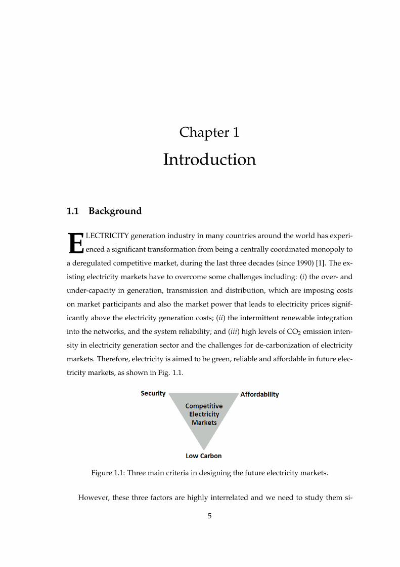
1.1 Three main criteria in designing the future electricity markets. . . . . . . . 5
2.1 Storage charging and discharging effects on supply/demand equilibriumpoint at a given moment in time (points 1 and 2 represent equilibriumpoint before and after storage installation). . . . . . . . . . . . . . . . . . . 38
3.1 Interconnected states in Australia’s National Electricity Market. . . . . . . 433.2 Dispatchable and intermittent electricity generation capacities in the NEM,
2017. . . . . . . . . . . . . . . . . . . . . . . . . . . . . . . . . . . . . . . . . 443.3 The clearing engine mechanism in the NEM (Source: AEMO). . . . . . . . 453.4 Calibrated linear, exponential and iso-elastic inverse demand functions at
price 50 $/MWh, demand 1500 MW, and elasticity -0.3. . . . . . . . . . . . 473.5 Comparing the simulation results (solid lines) of hourly price and demand
with the historical data (dashed lines) (Source: AEMO) for the average dayof 2017 in five states of the NEM. . . . . . . . . . . . . . . . . . . . . . . . . 48
4.1 Sorted historical data of hourly (a) electricity demand and (b) wind poweravailability in five regions of NEM during the year 2015. . . . . . . . . . . 61
4.2 Probability distribution of hourly prices in NEM and VIC, considering theclosure of coal power plant Hazelwood in VIC. . . . . . . . . . . . . . . . . 62
4.3 Probability distribution of daily peak prices in NEM and VIC, consideringthe closure of coal power plant Hazelwood in VIC. . . . . . . . . . . . . . . 63
5.1 SA’s Hourly wind power availability distribution in 2015 (the central marksshow the average levels and the bottom and top edges of the boxes indicatethe 25th and 75th percentiles). . . . . . . . . . . . . . . . . . . . . . . . . . . 82
5.2 Standard deviation and mean of hourly wholesale electricity prices in SAwith no storage. . . . . . . . . . . . . . . . . . . . . . . . . . . . . . . . . . . 83
5.3 Optimal strategic and regulated storage capacity for achieving differentprice volatility levels in SA region for a high demand day with coal-plantoutage. . . . . . . . . . . . . . . . . . . . . . . . . . . . . . . . . . . . . . . . 84
5.4 Daily peak and average prices in SA versus storage capacity in a high de-mand day with coal-plant outage. . . . . . . . . . . . . . . . . . . . . . . . 85
5.5 Square root of price volatility in SA versus storage capacity during a highdemand day with coal-plant outage. . . . . . . . . . . . . . . . . . . . . . . 86
xvii

5.6 Optimal regulated storage capacity versus the percentage of price volatil-ity reduction in the two-node market in a high demand day with coal-plantoutage in SA. . . . . . . . . . . . . . . . . . . . . . . . . . . . . . . . . . . . . 88
5.7 Square root of price volatility level in the 30-bus system after ten iterationsof Algorithm 1 with ∆Qst = 15MWh. . . . . . . . . . . . . . . . . . . . . . . 90
6.1 Mean (over 365 scenarios) wholesale electricity prices in VIC before andafter addition of only 5000 MWh regulated battery storage capacity. . . . . 107
6.2 Mean (over 365 scenarios) wholesale electricity prices in VIC before andafter addition of only 3125 MW regulated wind generation capacity. . . . . 108
6.3 The mean price, the square root of price volatility, and the life time rateof return for only regulated wind and only regulated battery allocationversus the equivalent annual budget in VIC. . . . . . . . . . . . . . . . . . 109
6.4 Normalized mean wholesale price and square root of price volatility fordifferent mixtures of regulated wind and regulated battery with the equiv-alent annual budget of 300 m$ in VIC. . . . . . . . . . . . . . . . . . . . . . 110
6.5 The budget allocation share between the regulated wind and the regulatedbattery as a function of the weighting factor k with the equivalent annualbudget of 300 m$ in VIC. . . . . . . . . . . . . . . . . . . . . . . . . . . . . 111
7.1 Normalized wind capacity availability (ωt) during off-peak, shoulder, andpeak load zones, distributed on [(1-σ)E(ω), (1+σ)E(ω)] with the given ex-pected value E(ω) . . . . . . . . . . . . . . . . . . . . . . . . . . . . . . . . . 125
7.2 Capacity investment Qtotal and its change ∆Qtotal due to carbon cap con-straint with coefficient φ ∈ 20, 40%. . . . . . . . . . . . . . . . . . . . . . 126
7.3 Carbon pricing for different CO2 emission reduction scenarios (φ ∈ 20 %,60 %). . . . . . . . . . . . . . . . . . . . . . . . . . . . . . . . . . . . . . . . 127
7.4 New capacity installation Qnew considering wind strategy (perfectly com-petitive and strategic). . . . . . . . . . . . . . . . . . . . . . . . . . . . . . . 127
7.5 New capacity installation considering remaining value. . . . . . . . . . . . 128
8.1 Normalized investment cost of generation and storage technologies dur-ing 2017-2052 (Normalization is compared to the costs in 2017). . . . . . . 148
8.2 Net increase/decrease of capacity for (a) generation and (b) storage andtransmission technologies by 2052 in NEM for different target levels ofemission intensity reduction. . . . . . . . . . . . . . . . . . . . . . . . . . . 149
8.3 The average yearly (a) wholesale prices and (b) net and wholesale de-mands in NEM, without or with emission reduction policy (net demand=wholesale demand + roof-top PV). . . . . . . . . . . . . . . . . . . . . . . 151
8.4 The trajectory of (a) carbon price, (b) carbon tax (positive) and subsidy(negative) of different generation types during 2017-2052. . . . . . . . . . . 152
8.5 The trajectory of fast response capacity tax (positive) and subsidy (neg-ative) for (a) No Emission Reduction policy, (b) 80% Emission IntensityReduction policy. . . . . . . . . . . . . . . . . . . . . . . . . . . . . . . . . . 153
xviii

8.6 Technology capacity mix in NEM with and without considering marketpower for (a) No Emission Reduction policy, (b) 80% Emission IntensityReduction policy. . . . . . . . . . . . . . . . . . . . . . . . . . . . . . . . . . 154
xix


List of Tables
4.1 Wholesale electricity prices $/MWh in five-node NEM market, consider-ing the closure of coal power plant Hazelwood in VIC. . . . . . . . . . . . 61
4.2 The annual electricity generation profit (billion$ per year) in five-nodeNEM market, considering the closure of coal power plant Hazelwood inVIC. . . . . . . . . . . . . . . . . . . . . . . . . . . . . . . . . . . . . . . . . . 63
4.3 Standard deviation of wholesale electricity prices $/MWh in five-nodeNEM market, considering the closure of coal power plant Hazelwood inVIC. . . . . . . . . . . . . . . . . . . . . . . . . . . . . . . . . . . . . . . . . . 64
4.4 Greenhouse gas emission of CO2 (million tonne per year) in coal and gas-fueled power plants in NEM, considering the closure of coal power plantHazelwood in VIC. . . . . . . . . . . . . . . . . . . . . . . . . . . . . . . . . 64
5.1 Location, capacity and generation cost of synchronous generators in the30-bus electricity system. . . . . . . . . . . . . . . . . . . . . . . . . . . . . 89
6.1 Wholesale electricity prices ($/MWh) in five-node NEM market in pri-mary and secondary cases. . . . . . . . . . . . . . . . . . . . . . . . . . . . . 106
7.1 The parameters for the inverse demand function. . . . . . . . . . . . . . . . 1247.2 Costs and technology specifications of generation firms. . . . . . . . . . . . 1247.3 Total CO2 emission every five years in the system with no carbon cap con-
straint. . . . . . . . . . . . . . . . . . . . . . . . . . . . . . . . . . . . . . . . 125
C.1 Financial and Technical Information on Intermittent Generators in NEM. . 167C.2 Financial and Technical Information on Synchronous Generators in NEM. 168C.3 Financial and Technical Information on Storage Technologies in NEM. . . 168C.4 Financial and Technical Information on Interconnectors in NEM. . . . . . . 168
xxi


Nomenclature
Indices
m Intermittent generation firm.
n Synchronous generation firm.
k Generation firm.
b Storage firm.
i, j Node.
y Investment period (yr).
t load time (hr).
w Scenario.
Parameters
αiyt, αitw, αit Intercept of the inverse demand function.
βiyt, βitw, βit Slope of the inverse demand function.
EICO2Y0
CO2 Emission intensity at base year Y0.
ECO2y CO2 Emission at year y.
φ Emission reduction coefficient.
EFni Emission factor of the synchronous generator.
αERy Emission intensity reduction target.
αsg,FRni Binary coefficient to distinguish fast response generators.
αst,FRbi Binary coefficient to distinguish fast response storage firms.
αFR Fast response proportion coefficient.
r Discount factor.
1
2
Qoldy′′ Old capacity of any generation, storage and transmission technol-
ogy installed at y′′, which is before the base year.
PL Plant life of any generation, storage and transmission technology.
cigmi,d
igmi Quadratic cost function coefficients of the intermittent generator.
γigmi Binary parameter to distinguish if the intermittent generator is strate-
gic/regulated.
Invigmiy Unitary investment cost of the intermittent generator.
Aigmit Energy availability coefficient of the intermittent generator.
ωkiystw, ωmitw Energy availability coefficient of the intermittent generator.
Cigmi Maximum potential capacity of the intermittent generator.
csgni Marginal operation and fuel cost of the synchronous generator.
γsgni Binary parameter to distinguish if the synchronous generator is
strategic/regulated.
Invsgniy Unitary investment cost of the synchronous generator.
Asgni Availability coefficient of the synchronous generator.
Rupni ,Rdn
ni Ramping up and down coefficient of the synchronous generator.
RAsgniy Energy availability limit of the synchronous generator at period y.
Invstf
biy Unitary investment cost of the storage on flow capacity.
Invstv
biy Unitary investment cost of the storage on volume capacity.
ηchbi ,ηdis
bi Charge and discharge efficiencies of the storage.
Astbi Availability coefficient of the storage.
ηtrij Efficiency of the transmission line.
Invtrijy Unitary investment cost of the transmission line.
Atrij Availability coefficient of the transmission line.
Prw Probability of scenario w.
∆ly,s,t length of time segment (y, s, t).
∆Yy length of time segment y.
∆Ss length of time segment s.
∆Tt length of time segment t.
Invk, mk, ck Investment, maintenance and operation cost of generator k.

3
σ Percentage of wind availability domain change.
Qig, Qsg, Qst, Qtr Intermittent generation, synchronous generation, storage and trans-
mission capacities.
Variables
Diyt, Ditw, Dit Electricity demand.
qigmiyt, qig
mitw, qigmit Generation of the intermittent generator.
qsgniyt, qsg
nitw, qsgnit Generation of the synchronous generator.
qstbiyt, qst
bitw, qstbit Electricity flow of the storage.
qtrijyt, qtr
ijtw, qtrijt Electricity flow from node j to node i.
Qig,newmiy New capacity of the intermittent generator.
Qsg,newniy New capacity of the synchronous generator.
qchbiyt, qch
bitw, qchbit Charge of the storage.
qdisbiyt, qdis
bitw, qdisbit Discharge of the storage.
Qstf,newbiy New flow capacity of the storage.
Qstv,newbiy New volume capacity of the storage.
Qtr,newijy New capacity of the transmission line.
Functions
Piyt (.) , Pitw (.) , Pit (.) Wholesale price.
Qigmiy(.) Total capacity of the intermittent generator.
Qsgniy(.) Total capacity of the synchronous generator.
Qstf
biy(.) Total flow capacity of the storage.
Qstv
biy(.) Total volume capacity of the storage.
Qtrijy(.) Total capacity of the transmission line.

Chapter 1
Introduction
1.1 Background
ELECTRICITY generation industry in many countries around the world has experi-
enced a significant transformation from being a centrally coordinated monopoly to
a deregulated competitive market, during the last three decades (since 1990) [1]. The ex-
isting electricity markets have to overcome some challenges including: (i) the over- and
under-capacity in generation, transmission and distribution, which are imposing costs
on market participants and also the market power that leads to electricity prices signif-
icantly above the electricity generation costs; (ii) the intermittent renewable integration
into the networks, and the system reliability; and (iii) high levels of CO2 emission inten-
sity in electricity generation sector and the challenges for de-carbonization of electricity
markets. Therefore, electricity is aimed to be green, reliable and affordable in future elec-
tricity markets, as shown in Fig. 1.1.
Figure 1.1: Three main criteria in designing the future electricity markets.
However, these three factors are highly interrelated and we need to study them si-
5

6 Introduction
multaneously. For instance, storage is expected to be installed in electricity networks to
increase the system reliability and decrease the average price and price volatility; closure
of coal power plants lowers the emission in the market but may lead to price increase
and volatility problem; although integration of wind and solar in power grids leads to
more clean electricity generation, it brings high levels of price volatility in the network;
although wind and storage both can remedy the high levels of average price and price
volatility in the market, their impacts on price reduction and volatility reduction are not
the same; and electricity generation technologies need to be taxed and subsidized at the
same time. Wind turbines need to be subsidized as they generate clean electricity and
need to be penalized as they bring intermittency in electricity networks.
Storage Integration in Power Grids:
Given the continuing decrease in battery costs, a large amount of battery storage ca-
pacity is expected to be installed in transmission and/or distribution networks in the
near future. Moreover, global roadmap vision indicates significant capacity increase for
pump-storage hydro power, from 140 GW in 2012 to 400 to 700 GW in 2050 [2]. Stor-
age can be used for multiple purposes including reduction in expensive peaking capac-
ity, managing intermittency of distributed wind/solar generation, and managing excess
generation from base-load coal/nuclear during off-peak times. By providing virtual gen-
eration capacity, storage may alleviate existing problems by reducing the impacts of in-
termittent power generation, market power, and volatility.
Coal Plant Closure and Price Volatility Problem:
The exercise of very high prices and price volatility can be the result of closing base-
load power plants down in electricity markets. In many countries, base-load coal power
plants are being closed due to either reaching their end of life, or being scheduled as part
of their national greenhouse reduction schemes [3]. In wholesale electricity markets with
high percentage of intermittent renewable generation, closure of base-load power plants
may lead to high electricity prices and increased volatility, which exposes the market par-
ticipants to a high level of financial risks. Over the past three years, four big coal-fueled

1.1 Background 7
power plants closed down in Australia’s National Electricity Market (NEM). The closure
of Victoria’s second biggest generator Hazelwood, with a 1600 MW capacity, in 2017 was
a highly debated topic in the press. The impact of a coal plant closure on market prices
can be measured in advance, which might be significant especially in highly renewable
penetrated networks.
Renewable Integration and Price Volatility Problem:
A high level of intermittent wind generation may also result in frequent high prices
and high levels of price volatility in electricity markets [4–6]. High levels of price volatil-
ity in a market refers to a situation in which the market prices vary in a wide range. For
example, one hundred hours with highest levels of electricity prices resulted in 21% of the
annual monetary market share in 2015 in South Australia, which is a highly price volatile
region in the NEM market [7]. Price volatility makes the task of price prediction highly
uncertain, which consequently imposes large financial risks on the market participants.
In the long term, extreme levels of price volatility can lead to undesirable consequences
such as bankruptcy of retailers [8] and market suspension. In a highly volatile electricity
market, the participants, such as generators, utility companies and large industrial con-
sumers, are exposed to a high level of financial risk as well as costly risk management
strategies [9]. In some electricity markets, such as the NEM, the market is suspended if
the sum of spot prices over a certain period of time is more than cumulative price thresh-
old (CPT). A highly volatile market is subject to frequent CPT breaches due to the low
conventional capacity and high level of wind variability. Storage, with price arbitrage
capability, can resolve the problem of high electricity prices and consequently it can pre-
vent high levels of price volatility. We note that recently a large scale storage installation
has been announced in South Australia for resolving the price volatility as well as the
reliability problems.
Average Price and Price Volatility Problem:
In addition to extreme levels of price volatility, high levels of average prices are also
undesirable in electricity markets. Closure of coal power plants and the fluctuation of gas

8 Introduction
price may result in high levels of average price and price volatility in electricity markets
[10]. For example, Australia’s National Electricity Market (NEM) has experienced very
high prices after the closure of Hazelwood coal power plant and the surge of gas price
[11]. As we discussed, price volatility imposes large financial risks on the market par-
ticipants by increasing the future price prediction uncertainty. On the other hand, high
levels of mean wholesale electricity prices lead to higher retail prices, i.e., impose high
cost on consumers.
One of the main reasons behind high electricity prices in highly concentrated elec-
tricity markets, such as NEM, is high levels of market power [7, 12]. Electricity markets
are less likely to be successful and stable in the presence of market power. When market
power is diagnosed to be persistent, more government intervention may pave the way
towards an efficient market as the private sector is likely to act slowly due to regulatory,
institutional, or other barriers [13]. In such cases, the government may choose to inter-
vene and install regulated wind and storage capacities, which have short construction
periods, to increase the competition in the market and reduce the market power as well
as the electricity prices [5].
Penalizing Carbon Emission and Supporting Dispatchable Capacity:
On the other hand, instead of controlling the firms, governments can influence the
market by setting effective tax and subsidy schemes. Market expansion models can be
used to design tax and subsidy schemes required to achieve long-term goals, like emis-
sion reduction strategies and maintaining reliability in the network.
In market expansion models for competitive power markets, electricity price is not set
by regulators but by the equilibrium between electricity supply and demand. In order to
make investment and operation decisions, generation companies have a strong interest
in modeling anticipated prices using available engineering and economic information.
They need appropriate decision making models considering not only technical operation
constraints but also the interaction among market participants. A variety of physical
and economic factors are included in market modeling, many of which are stochastic
by nature. Moreover, policy makers can intervene and incentivize the market players to

1.1 Background 9
meet their desired goals, such as caps on carbon emission.
Future electricity markets require to be green, reliable, and efficient. Greenhouse gas
reduction from power generation has been firmly on the political agenda recently, follow-
ing the international commitments under the Kyoto (1997) and Paris (2015) Agreements
[14]. The policies imposing an emission target level in the electricity sector affects many
existing fossil-fueled power plants as well as the future generation mix. Moreover, the
emission reduction policies may lead to massive investment in renewable generation.
High penetration of Variable Renewable Energy (VRE) in an electricity network can pose
challenges to system reliability. Additional fast response dispatchable capacity must be
introduced to the system to complement an increasing proportion of VRE generators
such as wind and solar photovoltaic [15]. This may lead to new obligations for VRE gen-
erators connected to NEM to ensure that the system reliability is maintained. Although
the decline in technology cost enables renewables to compete with fossil-fueled plants in
electricity generation, the incentive policies can be used to accelerate the ongoing transi-
tion toward a green network.
Australia’s National Electricity Market (NEM):
In the NEM, electricity is an ideal commodity which is exchanged between producers
and consumers through a pool. The market operator must ensure the agreed standards
of security and reliability. Security of electricity supply is a measure of the power system
capacity to continue operating despite the disconnection of a major generator or inter-
connector. In fact, unserved demand per year for each region must not exceed 0.002
percent of the total energy consumed. This level of reliability across the NEM requires a
certain level of reserve. However, when security and reliability is threatened, the market
operator is equipped with a variety of tools including demand side management, load
shedding and reserve trading to maintain the supply and demand balance.
Operating the NEM consists of estimating the electricity demand levels, receiving
the bidding offers, scheduling and dispatching the generators, calculating the spot price
and financially settling the market. Electricity demand in a region is forecasted based
on different factors, like population, temperature and sectoral energy consumption in

10 Introduction
that region. Electricity supply bids (offers) are submitted in three forms of daily bids,
re-bids and default bids [16]. Using the rising-price stack, generators are scheduled and
dispatched in the market.
1.2 Research Questions
In this thesis, we develop wholesale electricity market models to answer the following
research questions.
Research Question 1: How can we model strategic storage firms in a competitive
electricity market?
Large amounts of storage capacity are expected to be installed in power grids, which
impact the electricity prices at peak and off-peak times, and the electricity dispatch from
intermittent and classical generators in the market. In addition to generation and trans-
mission players, storage players impact the total amounts of electricity generation and
demand in an electricity market. We develop an electricity market model considering the
interaction between strategic storage firms with generation, and transmission players.
We address this research question and the related issues in Chapter 2.
Research Question 2: What is the impact of a coal plant closure on electricity prices
in a multi-region wholesale electricity market?
The prices may change from very high levels to low levels or vice versa as a conse-
quence of generation capacity closure (coal closure) or storage integration in a wholesale
electricity market. The existing electricity market models are mostly developed based
on linear inverse demand functions, which may not accurately indicate the relation be-
tween price and demand. Electricity market models including generation and storage
players with non-linear inverse demand functions exist in the literature as single-region
models. We develop multi-region wholesale electricity market models with non-linear
inverse demand functions, which can precisely capture the price and demand relation,
and use them to find the impact of a coal power plant closure on electricity prices in dif-

1.2 Research Questions 11
ferent nodes of an electricity market. We address this research question in Chapters 3 and
4.
Research Question 3: How can we find the optimal storage allocation to limit the
price volatility in a competitive electricity market?
The fast growing expansion of wind power generation may lead to extremely high
levels of price volatility in wholesale electricity markets. Storage capacities in electricity
networks in any form of pump-storage hydro, large scale or distributed batteries can help
to reduce the price volatility significantly in the market. It is important to find the opti-
mal size and location of required storage capacities, which can limit the price volatility in
an electricity market. Therefore, we develop an optimization model to solve the storage
allocation problem in a multi-region wholesale electricity market model including gener-
ation, storage and transmission players. We address this research question in Chapter 5.
Research Question 4: How can we find the optimal wind and storage allocation to
reduce the average price and price volatility in a competitive electricity market?
High levels of average price and price volatility in an electricity market can be the
consequence of a coal power plant closure or gas price fluctuation. Installing regulated
wind and storage capacities can lead to significant price and volatility reduction amounts
in the market. The impacts of wind and storage on the average price and on the price
volatility are different from each other. Therefore, we intend to develop an optimization
model to find the optimal wind and storage capacities in order to minimize the weighted
sum of average price and price volatility in the market. We address this research question
in Chapter 6.
Research Question 5: How can we calculate the required carbon price in a compet-
itive electricity market to limit the CO2 emission?
Carbon price in an electricity market provides incentives for carbon emission abate-
ment and renewable generation technologies. Penalizing carbon emission can signifi-
cantly impact the capacity planning decisions of both fossil-fueled and renewable gener-

12 Introduction
ators. We intend to calculate the amounts of carbon price or carbon tax that can fulfill an
emission abatement target in an electricity market. We address this research question in
Chapter 7.
Research Question 6: How can we design tax&subsidy incentive policies which
leads to a green and reliable electricity market?
Incentive schemes and policies play an important role in reducing carbon emission
from electricity generation sector. Emission abatement policies lead to more intermittent
renewable generation in the market, which may endanger the market reliability. There-
fore, in addition to setting incentive policies on emission reduction, we require another
set of policies to encourage more fast response dispatchable capacity to ensure the bal-
ance between supply and demand (reliability) at all times in the market. We intend to
calculate the incentive policies on emission and dispatchable capacities in order to tran-
sit towards a low carbon and reliable electricity market in long-term. We address this
research question in Chapter 8.
1.3 Literature Review and Research Gaps
In this thesis, we develop Cournot-based electricity market models with generation, stor-
age, and transmission players to address the market operation and planning issues re-
lated to designing a green, reliable and efficient electricity market. The literature review
on the research questions given in Section 1.2, and the corresponding research gaps are
discussed below.
Literature on Research Question 1: Cournot-based Electricity Market Models and
Storage Integration
Classical cost-minimization and surplus-maximization models for electricity gener-
ation do not incorporate strategic behaviors [1, 17]. Game theoretic models including
Cournot-Nash models are capable of computing market equilibrium considering strate-
gic behaviors, which originates from the players’ market power [18]. For example, a

1.3 Literature Review and Research Gaps 13
comprehensive analysis of Australian electricity sector in both least-cost and Cournot
schemes is discussed in [19], which states that the price bids may be significantly above
the marginal cost depending on the level of competition. Classical Cournot-based mod-
els are modified in the literature to study different affecting issues in electricity markets,
such as strategic interaction in electricity transmission networks [20], co-optimization
of ancillary services [21], joint evaluation of maintenance and generation strategies [22],
transforming energy-only markets to capacity-energy markets [23], considering volatile
renewable generation [7], and introducing storage players in the market [24]. Note that
Storage is modeled in a receding horizon problem in [25], in a double auction problem
in [26], and in a competitive electricity market model in [27], but not in a multi-region
Cournot-based electricity market model.
Therefore, to the best of our knowledge, the problem of modeling storage firms as
strategic players in multi-region Cournot-based electricity market models has not been
addressed before.
Literature on Research Question 2: Multi-region Cournot-based Electricity Market
Models
Electricity system modeling has changed significantly after the transformation of the
electricity industry from being a regulated monopoly to a deregulated competitive mar-
ket in many countries around the world [1]. Game-theoretical models have been exten-
sively used in imperfect competitive energy system analysis to calculate the price and
generation quantities in a market [28]. The problem of finding the equilibrium price and
generation in an electricity market, which consists of generation firms, transmission lines
and consumers, has been studied by solving the game-theoretical profit maximization
Cournot-based (quantity bidding) problems, e.g. in [7, 19–21, 23, 29–33], and Bertrand-
based (price bidding) or supply function-based problems, e.g. in [34–36]. However, the
multi-region non-cooperative electricity market models including non-linear inverse de-
mand functions have not been investigated in the literature.
The paper [29] studies a single-region electricity market in which firms compete in
quantity as in the Nash-Cournot game, and formulates the problem as a Linear Com-
14 Introduction
plementarity Problem (LCP). The paper [30] models the imperfect competition among
electricity producers as an LCP problem, in which the players consider the spacial price
discrimination to model the transmission lines in the market. The papers [20, 31] model
the transmission lines in electricity markets using a bi-level model in which strategic gen-
erators bid on their quantities in the upper level and a clearing engine with transmission
constraints clears the market in the lower level. Moreover, the multi-region electricity
market is formulated as a centralized convex optimization problem to make long-term
planning decisions [32], to include greenhouse gas reduction constraint [19], to introduce
capacity market beside an energy market [23], to analyze interrelated markets for differ-
ent commodities [21], and to observe the volatility of wind power [7]. The paper [33] for-
mulates a centralized convex optimization problem to find the price of carbon emission
in an electricity market. We note that these works are restricted to linear inverse demand
functions, which are the first order approximation terms at their nominal points and may
become imprecise approximations when the operational points change, for multi-region
market modeling.
The papers [34, 35] study the multi-region electricity market using a bi-level supply
function-based model in which the strategic generators bid on their supply function in
the upper level and a clearing engine with transmission constraints clears the market in
the lower level. The market participants strategically bid just on their prices in the upper
level of the market model in [36]. Although it is possible to extend the model formulation
in these works to consider non-linear inverse demand functions, they have to deal with
cumbersome computations pertaining to using the bi-level models.
To the best of our knowledge, the problem of solving a multi-region non-cooperative
electricity market with nonlinear inverse demand functions has not been addressed be-
fore.
Literature on Research Question 3: Storage Allocation in Wholesale Electricity
Markets
The problem of optimal storage operation or storage allocation for facilitating the in-
tegration of intermittent renewable energy generators in electricity networks has been

1.3 Literature Review and Research Gaps 15
studied in [37–44], with total cost minimization objective functions, and in [45–50], with
profit maximization goals. However, the price volatility management problem using op-
timal storage allocation has not been investigated in the literature.
The operation of a storage system is optimized, by minimizing the total operation
costs in the network, to facilitate the integration of intermittent renewable resources in
power systems in [37]. Minimum (operational/installation) cost storage allocation prob-
lem for renewable integrated power systems is studied in [38–40] under deterministic
wind models, and in [41] under a stochastic wind model. The minimum-cost storage al-
location problem is studied in a bi-level problem in [42,43], with the upper and lower lev-
els optimizing the allocation and the operation, respectively. The paper [44] investigates
the optimal sizing, siting, and operation strategies for a storage system to be installed in
a distribution company controlled area. We note that these works only study the mini-
mum cost storage allocation or operation problems, and do not investigate the interplay
between the storage firms and other participants in the market.
The paper [45] studies the optimal operation of a storage unit, with a given capacity,
which aims to maximize its profit in the market from energy arbitrage and provision of
regulation and frequency response services. The paper [46] computes the optimal supply
and demand bids of a storage unit so as to maximize the storage’s profit from energy ar-
bitrage in the day-ahead and the next 24 hour-ahead markets. The paper [47] investigates
the profit maximization problem for a group of independently-operated investor-owned
storage units which offer both energy and reserve in both day-ahead and hour-ahead
markets. In these works, the storage is modeled as a price taker firm due to its small
capacity.
The operation of a price maker storage device is optimized using a bi-level stochastic
optimization model, with the lower level clearing the market and the upper level maxi-
mizing the storage profit by bidding on price and charge/discharge in [48]. The storage
size in addition to its operation is optimized in the upper level problem in [49] when the
lower level problem clears the market. Note that the price bids of market participants
other than the storage firm are treated exogenously in these models. The paper [50] also
maximizes the day-ahead profit of a load serving entity which owns large-scale storage

16 Introduction
capacity, assuming the price bids in the wholesale market as exogenous parameters.
The paper [51] maximizes a large-scale energy storage system’s profit considering
the storage as the only strategic player in the market. Using Cournot-based electricity
market models, the generation and storage firms are considered as strategic players in
[24,29]. However, they do not study storage sizing problem and the effect of intermittent
renewables on the market.
Therefore, to the best of our knowledge, the problem of finding optimal storage ca-
pacity subject to a price volatility management target in electricity markets has not been
addressed before.
Literature on Research Question 4: Wind-Storage Allocation in Wholesale Electric-
ity Markets
The problem of storage allocation in the presence of intermittent renewable energy
generation in electricity networks has been studied in [37–39, 41–43], using cost mini-
mization modeling approaches, and in [24, 45–49], using profit maximization goals.
Facilitating the integration of renewable resources, the potential value of energy stor-
age in power systems with renewable generation is evaluated by minimizing the total
operation cost in the network in [37]. The optimal operation and sizing of the storage
systems is studied by minimizing the cost of the system in [39]. The storage allocation
in renewable integrated power systems is studied in [38] and [41] under deterministic
and stochastic wind models, respectively. To accommodate the integration of renewable
generation, bi-level optimization models are also proposed to determine the optimal al-
location and operation of energy storage systems in [42] and of battery energy storage
systems in [43], in which the upper level problem minimizes the storage system cost
and the lower level problem implements the power flow in the network. Note that these
works are based on cost minimization models and do not investigate the market interplay
between storage, renewable generators and other players.
Assuming the storage firms as price taker players in the market, the optimal operation
of storage firms in renewable integrated systems is determined by maximizing the profit
from energy arbitrage and regulation services in [45], by maximizing the energy arbitrage

1.3 Literature Review and Research Gaps 17
profit in day-ahead and hour-ahead markets in [46], and by maximizing their energy
and reserve profit in day-ahead and hour-ahead markets in [47]. Assuming the storage
firms as price maker players in the market, the optimal charge/discharge operation of the
storage devices, and the optimal operation and size of the storage devices are determined
in [48] and [49], respectively, treating the price bids of market participants other than the
storage players as exogenous inputs. The market operation behavior of all generation
and storage firms are considered endogenously in a single-node electricity market in [24]
using a Cournot-based electricity market model.
The charge/discharge behavior of storage firms and their impact on price volatility
reduction in a multi-region electricity market model is studied in [52]. However, studying
the joint effect of generation and storage on market price characteristics is missing in
the literature. As we show in Chapter 6, wind might be more efficient than storage in
reducing the average price and the results of [52] are not applicable when it is desirable
to reduce the average price in the market. Therefore, different from the existing work, we
consider the problem of managing the average price and the price volatility by optimal
allocation of wind and storage capacities.
To the best of our knowledge, the problem of optimal allocation of wind and storage
capacities for managing the average price and price volatility in the market has not been
addressed before.
Literature on Research Question 5: Carbon Pricing Using Long-term Generation
Expansion Models
Before electricity market deregulation, planning and operation scheduling were de-
pendent on administrative and centralized procedures. Cost minimization models have
been widely used in long-term capacity expansion models, e.g. planning in micro scale
[53] and in macro scale [54]. During the last three decades, power industry in many
countries and regions has transformed from being a centrally coordinated monopoly to a
deregulated liberalized market. Although classical cost minimization and surplus maxi-
mization models do not incorporate strategic behaviors existing in the markets [1], [17], a
heuristic cost minimization model is used for optimal investment planning in a compet-
itive market assuming different forecasted market price scenarios [55]. Game-theoretic
18 Introduction
models including Cournot-Nash are capable of computing market equilibrium, price and
generation, considering strategic behaviors. Cournot-based game models have been ex-
tensively used in energy systems analysis with formulations following the same logic,
e.g. in electricity markets [18] and global oil markets [28].
Research on short and long-term capacity expansion in electricity markets using game-
theoretic models has been conducted for a long time. Firms in the market compete by
deciding on their generation quantities and expansion-planning decisions in a Cournot
manner using an iterative solving algorithm [56] or a Mixed Linear Complementarity
Problem [29]. Since solving the Cournot-based market games as a LCP could be cum-
bersome, the problem of computing the Nash Equilibrium (NE) is posed as a centralized
optimization problem alternatively, e.g. on short term in [7] and on long-term in [19] and
[23].
Cournot-based models used in electricity market representation are mostly determin-
istic. By considering a set of scenarios, uncertainty on the conjectured price responses,
i.e., the slope of the linear inverse demand function, has been introduced in an oligopoly
Bayesian game where generation companies decide on their long-term generation and
capacity investment [32]. Uncertainties on both sides of supply and demand are con-
sidered in an oligopoly model in [57]. The load uncertainty is due to errors in the load
forecast, and the generator availability uncertainty is about generators that might have a
forced outage.
In both optimization and game-theoretic formulations, maximum carbon production
can be embedded in the model as a constraint [54], the dual variable of which indicates
the carbon price. In a cost minimization model, different values for maximum carbon
production limit calculates different dual variables or carbon prices.
To the best of our knowledge, the problem of designing carbon price policies required
to achieve long-term carbon cap targets in competitive electricity markets with strategic
generation players has not been addressed before.
Literature on Research Question 6: Designing Tax&Subsidy Policies Using Long-
term Market Expansion Models

1.3 Literature Review and Research Gaps 19
The problem of electricity market expansion for studying the future generation mix
or the CO2 emission abatement has been studied in [54,58–64], with least cost generation
expansion planning models, and in [19,23,29,32,33,65–67], with imperfectly competitive
market evolution models. However, the electricity market expansion problem with emis-
sion and fast response dispatchable capacity incentive policies has not been investigated
in the literature.
A least cost electricity generation expansion planning model, in which the total tech-
nology and operation costs to meet a specified demand are minimized, is studied in [58]
considering the demand side management, and in [59] considering the simultaneous ex-
pansion of the electricity and gas networks. A multi-period power generation expansion
model considering the CO2 emission target constraint is developed in [54, 60], which
calculates the additional costs of achieving a CO2 abatement target as the absolute and
marginal costs of abatement. Instead of embedding an emission target constraint, the
cost of CO2 emission is added to the fuel cost as carbon tax to support more renewable
power installation in [61].
Considering a target penetration level for renewables and an ensured payback period
constraints, the incentive rate (subsidy) on new renewable technologies are calculated in
[62]. Incentive policies for renewable energies and emission reduction are also calculated
using bilevel optimization models. Minimizing the total technology installation and op-
eration costs in the lower level problem in [63] (or maximizing the social welfare in the
lower level problem in [64]), the total policy intervention is minimized in the upper level
problem to calculate the incentive policies of renewable subsidization or carbon taxation.
In order to investigate the strategic (price making) behavior of market participants,
game-theoretical Cournot-based (oligopolistic) generation expansion models, i.e., market
evolution models, are developed, for instance in [29], and are compared with least cost
generation expansion models in [65]. Stochastic strategic generation expansion mod-
els are developed to include the uncertainty in conjectured-price response in [32] and
the uncertainty in renewable power availability in [66]. Moreover, strategic generation
expansion models have been utilized to manage the CO2 emission level in the market,
with an exogenous emission permit price in [67], and with a target emission constraint in

20 Introduction
[19, 33]. It is discussed in [33] that the dual variable of the emission target constraint can
be interpreted as the carbon price in the market.
The electricity market expansion models are also required to ensure that there is
enough dispatchable capacity connected to the network. In order to support more in-
vestment on dispatchable capacity, the total generation from wind and solar is limited to
30% of aggregated annual generation in each region in [54], and to incentivize the right
level of dispatchable capacity investment, capacity market is designed beside the energy
market in [23]. The Blueprint for the Future report [68] suggests to limit the total VRE
generation to a proportion of dispatchable generation in Australia in order to ensure the
system reliability and minimum required dispatchable capacity.
To the best of our knowledge, the problem of designing emission taxation and fast re-
sponse capacity support policies required to achieve long-term emission intensity reduc-
tion and dispatchability provision targets in competitive electricity markets with strategic
generation, storage and transmission players has not been addressed before.
1.4 Thesis Contributions
The contributions of this thesis to answer the research questions discussed are as follow-
ing:
• Contributions to answer Research Question 1 (in Chapter 2):
– A classical Cournot-based model of wholesale electricity markets is theoreti-
cally extended to embed storage firms as strategic players in the market.
– The game-theoretic game with strategic storage firms is developed and solved
as a centralized optimization problem. The Centralized version can be de-
veloped for Cournot-based game models which have linear inverse demand
functions.
• Contributions to answer Research Question 2 (in Chapter 3 and Chapter 4):
– A Cournot-based multi-region electricity market model with nonlinear inverse
demand functions is developed as a Mixed Complementarity Problem (MCP)

1.4 Thesis Contributions 21
to find the impact of a coal power plant closure on electricity prices. In this
model, generators are strategic and transmission lines are regulated.
– Transmission lines are modeled as individual market participants likewise the
other players in the game. In our model, we have strategic generation firms
and regulated transmission lines.
• Contributions to answer Research Question 3 (in Chapter 5):
– A bi-level optimization model is developed to find the optimal storage ca-
pacity required to limit the price volatility level in a multi-region electricity
market.
– The total storage capacity is minimized subject to a price volatility target con-
straint, in the upper level problem.
– The strategic interaction between generation, transmission and storage players
in the market is modeled as a stochastic (Bayesian) Cournot-based game with
exponential inverse demand functions, in the lower level problem.
– The existence of Bayesian Nash Equilibrium (Bayes-NE) is established for the
lower level problem, which includes exponential inverse demand functions.
• Contributions to answer Research Question 4 (in Chapter 6):
– A bi-level optimization model is developed to allocate a fixed budget opti-
mally between regulated wind and storage capacities to minimize the weighted
sum of average price and price volatility in an electricity market.
– In the upper level problem, the weighted sum of average price and price
volatility is minimized by allocating the fixed budget on regulated wind and
storage capacities in the market.
– In the lower level problem, the non-cooperative interaction between strategic
and regulated generation, storage and transmission players in the market is
modeled as a stochastic (Bayesian) Cournot-based game.
• Contributions to answer Research Question 5 (in Chapter 7):

22 Introduction
– A stochastic game-theoretic Cournot-based model is developed, in which strate-
gic and regulated generation firms decide on expanding their generation ca-
pacity considering an emission constraint and the uncertainties due to inter-
mittency of wind and solar.
– The dual variable of the emission cap constraint at the Bayes-NE point of the
game is used to calculate the carbon price required to limit the CO2 emission
to the cap level in the market.
– The remaining value of new technologies (their value at the end of the study
time) and the capacity retirement are considered in our model, which enables
us to calculate the capacity expansion/closure during the study period.
• Contributions to answer Research Question 6 (in Chapter 8):
– A game-theoretical Cournot-based electricity market expansion model is de-
veloped to find the future capacity mix of generation, storage and transmis-
sion in the market with both strategic and perfectly competitive (regulated)
players.
– All players in our model are subject to the emission intensity reduction con-
straint, the dual variable of which at the NE point is used to calculate the
emission tax and subsidy that generators pay and receive for a targeted low
emission market.
– All players in our model are also subject to the fast response dispatchable gen-
eration constraint, the dual variable of which at the NE point is used to calcu-
late the capacity tax and subsidy that generators and storage firms pay and re-
ceive for maintaining the system reliability (generation and demand balance).
1.5 Thesis Outline
Chapter 2: Game-theoretic Cournot-based Electricity Market Models with Storage
In Chapter 2, the mathematical formulation of a game-theoretic Cournot-based elec-
tricity market model is described. The market model includes several strategic and reg-

1.5 Thesis Outline 23
ulated generation firms and is extended as a multi-region model with strategic storage
players. After describing the mathematical formulations of AC and DC power flows,
the Cournot game in a wholesale electricity market is defined. The game is extended
to include strategic storage players and is solved as a centralized optimization problem.
Solving the game based on its Karush Kuhn Tucker (KKT) equations is also discussed in
this chapter.
Chapter 3: NEM as the Case Study
In Chapter 3, we introduce the NEM market briefly and explain its pricing mecha-
nism. The market clearing engine that settles the electricity generation, demand, and
price is discussed. Moreover, we discuss the price and demand curves in competitive
electricity markets based on linear and non-liner relations, and explain the calibration
mechanism of the inverse demand functions based on historical price and demand data
in the market. Then we show how accurate our model can simulate the electricity price
and demand levels in NEM.
Chapter 4: Impact of a Coal Power Plant Closure on a Multi-region Wholesale Elec-
tricity Market
In Chapter 4, the system model of a wholesale electricity market including strate-
gic/regulated generation, and transmission players is developed using a Cournot-based
electricity market model. Regarding the nonlinear inverse demand functions, the set of
KKT equations of market participants, i.e., wind and synchronous generators and trans-
mission players, is solved to find the NE solutions. Market simulation is repeated with
365 different scenarios to calculate the price volatility in the market. The NEM market is
studied as the case study and the impact of closing the Hazelwood power plant in Victo-
ria on the market prices and volatility is investigated. Greenhouse gas emission of CO2
in coal and gas power plants is also compared in simulations before and after the closure.
Chapter 5: Impact of Optimal Storage Allocation on Price Volatility in Electricity
Markets
In Chapter 5, a bi-level optimization model is proposed to find the nodal storage
capacities in an electricity market required to achieve a certain level of price volatility.
The price volatility is calculated at the Bayes-NE solution of a stochastic Cournot-based

24 Introduction
electricity market model including wind and synchronous generators, storage firms, and
transmission players. The set of KKT equations is solved to find the Bayes-NE solution
of the stochastic game and a greedy algorithm is used to solve the upper and lower level
problems. The NEM market is studied as the case study and the optimal capacity of
storage in South Australia and Victoria respect to a certain level of price volatility is cal-
culated. Our storage allocation framework is also applied to manage the price volatility
in a 30-bus IEEE system.
Chapter 6: Regulated Wind/Storage to Reduce the Electricity Market Price and
Volatility
In Chapter 6, a bi-level optimization model is proposed to allocate a fixed budget on
regulated storage and wind capacities in order to minimize the weighted sum of average
price and price volatility in a competitive market. A stochastic Cournot-based whole-
sale electricity market model is developed to find the Bayes-NE solution of the game
between intermittent and synchronous generators, storage firms, transmission lines, and
regulated wind and storage firm in the market. The set of KKT equations is solved to find
the market equilibrium solution and a line search algorithm is used to solve the upper
and lower level problems. The NEM market is studied as the case study and the optimal
capacity for regulated wind and storage firm is calculated to minimize the weighted sum
of price and volatility in the market.
Chapter 7: Long-Term Stochastic Planning in Electricity Markets Under Carbon
Cap Constraint
In Chapter 7, a long-term stochastic Cournot-based generation expansion model is
proposed, in which any generation firm maximizes the net present value of its profit sub-
ject to a aggregated CO2 emission constraint. The dual variable of the emission constraint
at the Bayes-NE point is used to calculate the carbon price required to limit the emission
in the market. Regarding the linear inverse demand functions, the game model is solved
as a centralized optimization problem. A generic wholesale electricity market including
coal, gas and wind generators is studied as the case study under several wind availabil-
ity scenarios. The effect of wind intermittency on capacity expansion decisions and on
carbon price is discussed in the simulations.

1.6 Publications 25
Chapter 8: Designing Tax&Subsidy Incentives Towards a Green and Reliable Elec-
tricity Market
In Chapter 8, a long-term Cournot-based market expansion model is proposed, in
which any generation, storage, and transmission firm maximizes the net present value
of its profit subject to an upper bound on CO2 emission intensity constraint and a fast
response dispatchable capacity constraint. The dual variable of the emission constraint at
the NE point is used to calculate the tax and subsidy incentive policies required to reduce
the emission intensity and the dual variable of the dispatchable capacity at the NE point is
used to calculate the tax and subsidy policies required to ensure the existence of adequate
dispatchable capacity in an electricity market with high level of intermittent generation.
The set of KKT equations are analyzed to calculate the tax and subsidy policies. The
NEM market is considered as the case study and the required tax and subsidy policies
are calculated to enable the transition towards a green and reliable electricity market by
2052 in Australia.
1.6 Publications
The outcomes of this thesis are published or under review for publication in the following
journals and conferences.
• Journals:
– Masoumzadeh, A., Nekouei, E., Alpcan, T., & Chattopadhyay, D. (2017). Im-
pact of Optimal Storage Allocation on Price Volatility in Energy-only Electric-
ity Markets. IEEE Transactions on Power Systems, vol. PP, no. 99, pp. 1-1,
2017. (Chapter 5)
– Masoumzadeh, A., Nekouei, E., & Alpcan, T. Regulated Wind-Storage Alloca-
tion to Reduce the Electricity Market Price and Volatility, submitted to IEEE
Transactions on Power Systems. (Chapter 6)
– Masoumzadeh, A., Alpcan, T., & Nekouei, E. Designing Incentive Policies To-
wards a Green and Reliable Electricity Market, submitted to IEEE Transactions

26 Introduction
on Power Systems. (Chapter 8)
• Conferences:
– Masoumzadeh, A., Nekouei, E., & Alpcan, T. (2017, September). Impact of a
Coal Power Plant Closure on a Multi-region Wholesale Electricity Market. in
2017 IEEE PES Innovative Smart Grid Technologies Conference Europe (ISGT-
Europe), Sept 2017, pp. 16. (Chapter 4)
– Masoumzadeh, A., Nekouei, E., & Alpcan, T. (2016, November). Long-term
Stochastic Planning in Electricity Markets under Carbon Cap Constraint: A
Bayesian Game Approach. In Innovative Smart Grid Technologies-Asia (ISGT-
Asia), 2016 IEEE (pp. 466-471). IEEE. (Chapter 7)

Part I
Electricity Market Models and NEMas the Case Study
27


Introduction to Part I 29
Introduction to Part I
ELECTRICITY market models are developed to find the electricity market prices
based on the interaction between market players. Classical electricity market mod-
els just include generation players, who aim to maximize their profit considering the
transmission constraints in the network. The classical electricity market models are ex-
tended in this thesis because of the integration of storage firms, in small or large scales.
In Chapter 2, we introduce a classical Cournot-based electricity market model, in
which we discuss the generation and transmission players explicitly. We extend the
model by embedding the storage firms as strategic players in the market. The impact
of storage energy flow on market prices is compared in charging and discharging situa-
tions. This electricity market model is used as part of the models in other chapters.
In Chapter 3, we first introduce the NEM market as the case study for our simulations
in this thesis and explain how the market clearing engine settles the electricity generation,
demand and price in the NEM. Then, we explain the inverse demand function calibra-
tion methodology, and compare the linear and non-linear inverse demand functions with
each other. We also show how accurate our model can simulate the electricity price and
demand levels in NEM.


Chapter 2
Game-theoretic Cournot-basedElectricity Market Models with
Storage
Existing wholesale electricity markets have been designed for the traditional electricity grid that has
very limited storage capability. In the near future, a substantial amount of storage capacity is expected
to be installed in power grids following the decentralization and renewable distributed generation
trends. At the same time, information and communication technologies enable aggregation of storage
capabilities regardless of their specific form which can be, e.g. pump-storage hydro, large-scale or
distributed residential batteries, or electric vehicles. In this chapter, a classical Cournot game model
is extended in order to analyze how strategic storage firms can be modeled in an electricity market
and influence the wholesale price levels during charging and discharging periods. The developed
model takes power generators (synchronous and intermittent), storage firms and transmission lines
as market players into account, and is used as part of the developed models in the other chapters.
2.1 Introduction
In this chapter, a classical Cournot-based electricity market model is extended by embed-
ding strategic storage firms which can be considered as owners of virtual power plants.
Our model considers synchronous and renewable generators, storage firms and trans-
mission lines in a multi-region electricity market. Any player maximizes its utility in
the game, assuming linear price (inverse demand) functions. Note that the solution of
individual players’ profit maximization problems, the Nash Equilibrium solution of the
game, can be found by solving a single optimization problem or a Mixed Complemen-
tarity Problem (MCP). Because the inverse demand functions in our model are linear, we
31

32 Game-theoretic Cournot-based Electricity Market Models with Storage
can model the electricity market as a centralized optimization problem.
The contributions of this chapter include the following:
• We theoretically extend a classical multi-period Cournot-based electricity market
model by introducing storage firms, who own virtual power plants, as strategic
players in the market.
• We solve our extended Cournot-based electricity market model as a centralized op-
timization problem. Note that the centralized version just applies to market models
with linear inverse demand functions.
The rest of this chapter presents the AC and DC power flow models in Section 2.2,
the wholesale electricity market game model in Section 2.3, and ends with a conclusion
in Section 2.5.
2.2 Mathematical Model Description
AC Power Flow
Power flow equations (2.1) describe the steady-state behavior in an electric power grid.
At point or bus i, the nominal power injected to the network, Snominali , consists of active
power, Pactivei , and reactive power, Qreactive
i . The voltage level at bus i, Vi, and the current
injected to the network from the bus i, Ii, are as:
Snominali = Pactive
i + jQreactivei = Vi I∗i ∀i (2.1)
Pactivei − jQreactive
i = V∗i Ii = V∗i ∑j
YijVj, ∀i, (2.2)
where Yij denotes the admittance between bus i and j, and (.)* denotes complex conjuga-
tion.
Accordingly, the active and reactive powers correspond to the real and imaginary

2.2 Mathematical Model Description 33
parts of the nominal power, respectively, as:
Pactivei = ReV∗i ∑
jYijVj ∀i
Qreactivei = −ImV∗i ∑
jYijVj ∀i
Considering the phasor type of the voltage Vi with the voltage absolute |Vi| and the
voltage phase δi as Vi = |Vi|ejδi , and the admittance elements Y with their conductance
amounts G and susceptance amounts B as Yij = Gij + jBij, we can write the final power
flow equations as:
Pactivei = ∑
j|Vi||Vj|(Gijcosδij + Bijsinδij), ∀i,
Qreactivei = ∑
j|Vi||Vj|(Gijsinδij − Bijcosδij), ∀i,
where δij denotes δi − δj.
DC Power Flow
Direct Current Load Flow (DCLF) provides estimates of line power flows on AC power
systems. As a simplification, DCLF looks only at the active power and neglects the reac-
tive power [69].
DC load flow analysis has four basic assumptions:
• Line resistances (active power losses) are negligible i.e. in line impedance Z we assume
that Re(Z) Im(Z).
• Voltage angle differences are assumed to be small i.e. sin(δ) ' δ and cos(δ) ' 1.
• Magnitudes of bus voltages are set to 1.0 per unit (flat voltage profile, Vrated).
With the simplified AC power equations under the assumptions made above, the

34 Game-theoretic Cournot-based Electricity Market Models with Storage
active power flowing from node i to node j can be shown as:
Ptrji = |Vi|(Gij|Vi| − Gij|Vj| cos δij − Bij|Vj| sin δij)
' |Vrated|2(−Bijδij) ∀i, j(2.3)
which is used in our developed electricity market model to show the power flow on
interconnectors.
Note that we rename the active power Pactive to q in the remainder of Chapter 2.
2.3 Game-theoretic Model of a Wholesale Electricity Market
Power suppliers in a competitive electricity market generate power in order to maximize
their profits. Players in a generic strategic (non-cooperative) game are either able to af-
fect the price by deciding on their generation quantities, which are referred to as strategic
players, or just follow the price in the market, which are referred to as perfectly competi-
tive (price-taking) players. Accordingly, we define the following Cournot-based game to
model the electricity generation behavior in a wholesale electricity market.
2.3.1 Game Definition and Nash Equilibrium:
Let K = 1, · · · , K be the set of generation firms participating in the electricity mar-
ket. At time t ∈ T , T = [1, · · · , T], they decide on their electricity generation qgt =
[qg1,t, · · · , qg
K,t] < 0. We assume that the generator k has constant marginal cost of produc-
tion ck ≥ 0.
The price P determines per unit revenue of a firm in the market. Inverse demand or
pricing function, Pt(Dt), is defined by a linear equation with parameters αt and βt, and is
determined by the market demand, Dt, that has to match the total generation, ∑k qgk,t, in
a one-node model:
Pt(Dt) = αt − βtDt. (2.4)
The demand function parameters α and β are calculated based on the historical price and
demand data in the region.

2.3 Game-theoretic Model of a Wholesale Electricity Market 35
Players in the model are categorized into perfectly competitive and strategic ones,
which differ in their objective functions. A strategic player (generator) decides on its
generation qgk,t according to the following objective function:
Ugk = ∑
tqg
k,tPt(Dt)− ckqgk,t. (2.5)
while the perfectly competitive or regulated generator’s objective function is:
Ugk = ∑
tqg
k,tPt(Dt) + βtqgk,t − ckqg
k,t (2.6)
Due to the term βtqgk,t, the perfectly competitive player never withholds its available
capacity to raise the market price, i.e. it does not have or misuse the market power ability
to strategically increase the wholesale prices.
Definition 1. A perfectly competitive (PC) player does not misuse or have the market power to
raise wholesale prices, while a strategic player may deliberately decide to increase the prices by
withholding its available capacity.
Considering all firms strategic, the generation firm k solves the following profit max-
imization problem:
maxqg
k,t≥0Ug
k (qg) := ∑
tqg
k,tPt(qgt )− ckqg
k,t s.t. Agqg ≤ bg (2.7)
where generation constraints are embedded in the inequality Aqg ≤ b. The action space
of the generation players is defined as Ω = qg ∈ R+K∗T |Agqg ≤ bg, which is com-
pact, convex, and non-empty in our model. Moreover, as the quadratic objective function
is concave and continuous on its action set, the problem (2.7) is a convex optimization
problem.
The problem (2.7) has the corresponding Lagrangian function,
Lk = ∑t(αt − βt ∑
k′qg
k′,t)qgk,t − ckqg
k,t − λ(Agqg − bg),
where λ ≥ 0 is the vector of Lagrange multipliers.

36 Game-theoretic Cournot-based Electricity Market Models with Storage
Consequently, the Karush-Kuhn-Tucker conditions are both necessary and sufficient
for optimality [70],
dLk
dqgk,t
= αt − βt ∑k′
qgk′,t − βtq
gk,t − ck − λa(k ∗ t) = 0, (2.8)
where a(k ∗ t) is the (k ∗ t)th column of the constraint matrix Ag. The solution of (2.8)
is the best response of player or generation firm k given the decisions of other players.
The intersection of the best responses of all players, qg∗, is by definition the NE of the
corresponding strategic game G = K, qg ∈ Ω, Ug.
Proposition 1. The electricity generation strategic game G = K, qg ∈ Ω, Ug played among
the set of K firms, which decide on generation levels qG in order to maximize the profit Ug admits
a Nash Equilibrium solution qg∗ if the action space Ω = qg ∈ R+K∗T |Agqg ≤ bg given
coefficient matrix Ag and vector matrix bg is convex, compact, and non-empty. Furthermore, any
solution qG∗ of the quadratic optimization problem
maxqg≥0
F := ∑k,t
(αt −βt
2 ∑k′
qgk′,t)q
gk,t −
βt
2(qg
k,t)2 − ckqg
k,t
s.t. Agqg ≤ bg
is a NE of the game.
Proof. The proof follows the Theorem 4.4 in [7] and [71].
2.3.2 The Game with Strategic Storage Firms
We call a firm that operates a set of storage capacities, e.g. battery or pump-storage
hydro, in the network a storage firm. The firm’s operation mode can be either charging or
discharging. While charging, the storage generates electricity similar to the conventional
generators, and while discharging, it operates as an additional load in the system. Having
generation (Discharging) and demand (charging) modes, a storage firm does not look like
conventional generators modeled in the market.

2.3 Game-theoretic Model of a Wholesale Electricity Market 37
A strategic storage player with decision variable qstt is modeled and embedded in
our non-cooperative electricity generation game. Storage facilities are limited by their
charging rate and capacity constraints [72]. According to the charging rate constraint,
discharging takes positive values 0 ≤ qstt ≤ qst,max, and charging takes negative val-
ues qst,min ≤ qstt ≤ 0. In order to satisfy the capacity constraints, the actual charg-
ing level, with initial value of Qst,0, must be maintained within a proper range, i.e.,
0 ≤ Qst,0 −t
∑t′=1
qstt′ ≤ Qst,max, where t ∈ T .
While discharging, the storage firm injects electricity into the grid. Therefore, its dis-
charging adds to total generation, which is equal to the total demand: yt = ∑k qgk,t + qst
t ,
if qstt ≥ 0. Given the inverse demand function in (2.4), the utility function of the storage
firm, Ustt = Ptqst
t , becomes:
Ustt = (αt − βt(∑
kqg
k,t + qstt ))q
stt i f qst
t ≥ 0 (2.9)
On the other hand, storage charging results in changing the intercept coefficient in the
inverse demand function, i.e., Pt = (αt − βtqstt )− βtDt, if qst
t < 0. While charging, given
the total generation of incumbent generators, ∑k
qgk,t, the utility function of the storage
firm, Ustt = Ptqst
t , considering the new inverse demand function is:
Ustt = ((αt − βtqst
t )− βt ∑k
qgk,t)q
stt if qst
t < 0. (2.10)
Note that the terms in these utility functions are identical and instead of looking at a
storage firm in discharging and charging modes, we can consider the strategic storage
firm in a non-cooperative electricity generation game as a generator with both positive
and negative bids (generation).
Therefore, it is acceptable to assume a storage firm as a generator with real decision
variable, i.e., a generator capable of generating both positive and negative amounts. Fig-
ure 2.1 illustrates how storage charging/discharging affects the supply curve, while the
demand curve is assumed fixed, and shifts the equilibrium point.
Due to extension of the game for multiple strategic storage players, the objective func-

38 Game-theoretic Cournot-based Electricity Market Models with Storage
Figure 2.1: Storage charging and discharging effects on supply/demand equilibriumpoint at a given moment in time (points 1 and 2 represent equilibrium point before andafter storage installation).
tion of storage firm b and generator firm k respectively become:
Ustb (q
g, qst) = ∑t
qstb,t(αt − βt(∑
kqg
k,t + ∑b
qstb,t)) (2.11)
Ugk (q
g, qst) = ∑t
qgk,t(αt − βt(∑
kqg
k,t + ∑b
qstb,t))− ckqg
k,t (2.12)
Consequently, the NE point of the new game including strategic storage players can
be computed by solving the modified centralized optimization problem:
max ∑t(αt −
βt
2(∑
kqg
k,t + ∑b
qstb,t))(∑
kqg
k,t + ∑b
qstb,t)−
βt
2(∑
kqg
k,t2+ ∑
bqst
b,t2)−∑
kckqg
k,t
(2.13)
s.t. [ Ag Ast ][qg
qst] ≤ [
bg
bst]
Based on the results in Proposition (1), the Lagrangian equations for the optimization
problem (2.13) respect to variables qg and qst coincidence with Lagrangian equations for
individual profit maximization problems of storage firms with utility function (2.11) and
generators with utility function (2.12). Hence, the solution of (2.13) coincides with the
NE of the game.
In order to consider energy flow efficiency for charging and discharging, 0 ≤ µdis, µch ≤
1, it needs to allocate two independent positive variables qchb,t and qdis
b,t for storage charge
and discharge quantities. Again, the net energy flow of storage firm b at time t, qstb,t =

2.4 Multi-nodal, Multi-period Wholesale Electricity Market 39
qdisb,t µdis − qch
b,tµch , takes a real value. However, for simplicity we assume no energy loss for
storage firms and continue only with the variable qstb,t.
2.4 Multi-nodal, Multi-period Wholesale Electricity Market
2.4.1 The Game as a Centralized Optimization Problem
The multi-period (finite horizon) wholesale electricity market model presented can be ex-
tended at multiple interconnected nodes by inserting the node index i ∈ I , I = [1, · · · , I].
In a multi-nodal game, the transmission value between the nodes i and j emerges as an
independent variable qtrij,t which needs to be decided on in the game. Given the transmis-
sion player between nodes i and j) behaves perfectly competitive, according to Definition
(1) and similar to (2.6) it has the utility function:
Utrij = ∑
t(Pi,t − Pj,t)qtr
ij,t +β j,t + βi,t
2(qtr
ij,t)2
where the player transmits electricity from the higher price node to the lower price node
as long as either there is price difference between nodes i and j or the transmission line is
congested. The second term, β j,t+βi,t2 (qtr
ij,t)2, differentiates the player from a strategic one
and prevents withholding the available capacity to benefit strategically from the price
difference between nodes.
On the other hand, when the transmission player between nodes i and j behaves
strategically, similar to (2.5) it has the following utility function:
Utrij,t = ∑
t(Pi,t − Pj,t)qtr
ij,t
where it is capable of increasing the price differences strategically by withholding its
available capacity.
Players of the game are categorized into: (1) Generation firms, (2) Storage firms, (3)
Transmission firms, which can be either strategic or regulated. The generation firm k
in node i decides on the vector of variables [qgk,i,1, · · · , qg
k,i,T] which take positive values,

40 Game-theoretic Cournot-based Electricity Market Models with Storage
whereas the storage firm b in node i decides on the vector of variables [qstb,i,1, · · · , qst
b,i,T]
which take both positive and negative values, and the transmission firm between nodes
i and j decides on the vector of variables [qtrij,1, · · · , qtr
ij,T] which take both positive and
negative values as well.
The mathematical model presented below is an extension of the centralized optimiza-
tion problem (2.13), which is developed for the energy-only five node NEM market sub-
ject to generation, storage and transmission constraints. The network constraints are
given based on DC load flow (DCLF) assumptions (the Kirchoffs law is always respected
in our models). The multi-nodal intertemporal wholesale electricity market model con-
sisting of strategic generations and storage firms and regulated transmission lines is:
maxqg,qtr,δ,D0
qst
∑i,t
(αi,t −βi,t
2Di,t)Di,t −∑
k,i,tck,iq
gk,i,t − (∑
k,i,t
βi,t
2qg
k,i,t2+ ∑
b,i,t
βi,t
2qst
b,i,t2) (2.14a)
s.t.
Di,t = ∑k
qgk,i,t + ∑
bqst
b,i,t −∑j
qtrji,t ∀i, t (2.14b)
qtrji,t = |Vrated|2(−Bijδij,t) ≤ Qtr
ji ∀i, j, t (2.14c)
δmini ≤ δi,t ≤ δmax
i ∀i, t (2.14d)
qgk,i,t ≤ Qg
k,i ∀k, i, t (2.14e)
qgk,i,t − qg
k,i,t−1 ≤ Rupk,i Qg
k,i ∀k, i, t (2.14f)
qgk,i,t−1 − qg
k,i,t ≤ Rdnk,i Qg
k,i ∀k, i, t (2.14g)
qgk,i,t ≤ ωk,i,tQ
gk,i ∀k, i, t (2.14h)
∑t
qgk,i,t ≤ RAg
k,i ∀k, i (2.14i)
0 ≤ Qst,0 −t
∑t′=1
qstt′ ≤ Qst ∀b, i, t (2.14j)
qst,minb,i ≤ qst
b,i,t ≤ qst,maxb,i ∀b, i, t (2.14k)
where qg, qst, qtr are independent variables, and Di,t, δij,t are intermediate variables.
The optimization problem (2.14a)-(2.14k) considers all individual profit maximization

2.4 Multi-nodal, Multi-period Wholesale Electricity Market 41
problems. As shown in Proposition 1, the objective function (2.14a) enables us to write
the game as a centralized optimization problem. Constraint (2.14b) show the nodal elec-
tricity supply and demand balance. Constraint (2.14c) presents the electricity transmitted
between nodes (where |Vrated| is the rated voltage assumed in the network, Bij is the sus-
ceptance characteristic of the line and δij, i.e., δi − δj, is voltage phase difference between
nodes i and j) and limits the transmission values to the maximum power flow capacities.
As the problem is on DCLF format, constraint (2.14d) expresses the technical limit just on
voltage phases and does not consider the voltage magnitudes. The generation capacity
limit is shown in (2.14e). Constraints (2.14f)-(2.14g) show the ramp limits of generators
while the problem is cast as a chronological one. Period-by-period availability limit ap-
plicable to all generators especially intermittent wind turbines are shown in (2.14h), and
intertemporal generation limits due to fuel scarcity or planned/forced outages are ex-
pressed in (2.14i). Considering the strategic storage players, we include the constraints
(2.14j)-(2.14k) to show the storage capacity and the charging rate limit, respectively.
2.4.2 The Game as a Mixed Complementarity Problem
Alternatively, we can solve the electricity market game using the best response functions
of all firms participating in the market. The best response of any player satisfies the
necessary and sufficient Karush-Kuhn-Tucker (KKT) conditions. The KKT conditions, i.e.
the set of first order optimality equations of all players, are the derivative of Lagrangian
function of each player L respect to all its decision variables, e.g. q:
∂L∂q≤ 0 ⊥ q ≥ 0 if q ≥ 0 (2.15a)
∂L∂q
= 0 if q is free (2.15b)
where the perpendicularity sign, ⊥, indicates that one of the adjacent inequalities must
at least be satisfied as an equality [73], i.e., the complementarity constraints.
Then, any intersection of all firms’ best response functions will be a NE. At the NE
strategy of the game, no player has any incentive to unilaterally deviate its strategy from

42 Game-theoretic Cournot-based Electricity Market Models with Storage
the NE point. The KKT equations of the game are fully described in Chapter 5.
2.5 Conclusion
Electricity networks are transforming toward installing substantial amounts of storage in
different forms of pump-hydro, large-scale batteries and distributed batteries as a buffer
system to store the excess generated electricity at off-peak hours and sell it to network
at peak hours. We developed a multi-region Cournot-based wholesale electricity market
model and embedded the storage in it with the following conclusions:
• Storage players can be modeled as generators with both positive and negative gen-
eration amounts in the market. In other words, although storage charging impacts
the inverse demand functions on the demand side, we can equivalently find the
storage impact on the supply side.
• Transmission lines are also modeled as individual players in our model, who max-
imize their utility in the game. Considering a market power term, we have both
strategic and regulated transmission players in our model.
• Given linear inverse demand functions in our Cournot-based electricity market
model, we transform the game model into a centralized version and solve it as
an optimization problem to find the NE solution.
• When there is a nonlinear inverse demand function in a Cournot-based market
model, the best responses of all players must be written as the set of KKT equa-
tions to find the NE solution of the game.
The electricity market model developed in this chapter is used as part of the models
in other chapters.

Chapter 3
NEM as the Case Study
3.1 Overview of National Electricity Market (NEM)
The Australia’s National Electricity Market (NEM) operates as a wholesale market for the
supply of electricity to retailers and end-users. NEM is operated by Australian Energy
Market Operator (AEMO) and consists of five interconnected regions (states) shown in
Fig. 3.1: South Australia (SA), Queensland (QLD), Tasmania (TAS), Victoria (VIC) and
New South Wales (NSW).
Figure 3.1: Interconnected states in Australia’s National Electricity Market.
In NEM 2017, different types of electricity generation firms, i.e. coal, gas, hydro and
wind, with a total (both dispatchable and intermittent) generation capacity of 45.7 GW are
active. Roof-top solar with capacity of 4.8 GW is also generating electricity in Australia.
Fig. 3.2 illustrates the existing generation capacities in the NEM, which are used in our
43

44 NEM as the Case Study
numerical simulations and are gathered from AEMO’s website (aemo.com.au).
States in AustraliaSA QLD TAS VIC NSW
GW
0
2
4
6
8
10
12Generation Capacities in Australia's National Electricity Market
CoalGasHydroWindPV
Figure 3.2: Dispatchable and intermittent electricity generation capacities in the NEM,2017.
In market NEM, 13, 23, 21, 20, and 18 synchronous generators are participating in SA,
QLD, TAS, VIC, and NSW, respectively. The NEM also includes the total wind power
capacities of 1250 MW in SA, 0 MW in QLD, 250 MW in TAS, 964 MW in VIC, and 554
MW in NSW. The share of wind power installed capacity in total electricity generation
capacity is 34.3% in SA, 0% in QLD, 9.1% in TAS, 8.7% in VIC, and 3.4% in NSW. SA
possesses the highest share of wind power in its total electricity generation in NEM.
In the NEM, electricity is an ideal commodity which is exchanged between producers
and consumers through a pool. Wholesale trading of electricity is conducted in a spot
market. Generators offer to supply the market with specific amounts of electricity at
particular prices. Offers are submitted every five minutes (market price cap is 11000
$/MWh and market floor price is -1000 $/MWh). Finally, the output from all generators
is aggregated and scheduled to meet the demand.
Fig. 3.3 illustrates the clearing engine mechanism in the NEM. Bids to produce elec-
tricity received by AEMO are stacked for each dispatch period in ascending price order.
Generators are scheduled into production to meet the demand with the least-cost gener-

3.2 Calibrating the Inverse Demand Functions 45
ation option. Note that the spot price for each trading period (half hour) is calculated as
the average of the six dispatch prices (every five minutes).
Figure 3.3: The clearing engine mechanism in the NEM (Source: AEMO).
Electricity trade between two regions helps to lower the price difference between
those regions. The interconnectors in NEM are either regulated or unregulated. Regu-
lated interconnectors have passed the Australian Competition and Consumer Comission
(ACCC) devised regulatory test and are eligible to receive fixed annual revenue, but un-
regulated ones derive revenue by trading in the spot market. All interconnectors in NEM
are regulated, while Tasmania is connected via an unregulated interconnector to Victoria.
The inteconnetor capacities existing in NEM are listed in Table C.4 in Appendix C.
3.2 Calibrating the Inverse Demand Functions
In economic theory, price relates to demand in a function called the demand curve. In
this thesis, We have calibrated the inverse demand curves based on NEM’s historical
price and demand data with both linear and non-linear functions.
Two most commonly used inverse demand functions in microeconomics literature
are the linear and iso-elastic models [74], e.g., in [24, 28]. Exponential inverse demand
function has also been used in energy market models [75]. The inverse demand func-
tion of most commodities follows a non-linear downward sloping price versus demand
relation [76] and a linear inverse demand function is just its first order approximation

46 NEM as the Case Study
at an operating price and demand level. The linear function may become invalid when
the operating point changes drastically, e.g., when the price plunges from the very high
amount of 11000 $/MWh to low level of 50 $/MWh.
The iso-elastic and exponential functions can more accurately illustrate the price and
demand relation. In fact, the exponential function, p = α′e−β′q, is the modified version of
the iso-elastic function, ln(p) = α− βln(q) or p = αe−βln(q) with α = eα, which substitutes
the logarithmic demand levels with nominal levels. We discuss three reasons privileging
the exponential inverse demand function over the iso-elastic. Firstly, the KKT conditions
(first order optimality conditions) of our developed market game models become highly
non-linear under the iso-elatsic function and it becomes hard to numerically solve them.
The derivative of the exponential inverse demand function with respect to demand is∂p∂q = −β′p, while the derivative of the iso-elastic function respect to demand is ∂p
∂q =
−βpq−1. Secondly, the exponential function has a finite price feature while the iso-elastic
function goes to infinity for small levels of demand. Lastly, the exponential function
partially covers the specifications of both linear and iso-elastic functions. Consequently,
we use and calibrate exponential inverse demand functions to characterize the price and
demand relations in our models in Chapters 4, 5 and 6.
In electricity market models, the constant coefficients in the inverse demand func-
tions are usually calibrated based on actual price/demand data , p/q, and price elasticity
levels, ε =∂qq
∂pp
[76], which are given as input to our models. Given two equations of price-
demand function and elasticity function, i.e., p = f (q) and ε = ∂q∂p
pq , and two unknowns,
we can find the both parameters in all three discussed inverse demand functions. For
instance, given the price of p = 50 $/MWh, demand of q = 1500 MW and price elas-
ticity of demand ε = −0.3, the linear function p = 6503 −
19 q, the iso-elastic function
ln(p) = 28.28− 103 ln(q), and the exponential function p = 50e
103 e−
1450 q can be extracted.
Fig. 3.4 compares the calibrated linear, exponential and iso-elastic inverse demand func-
tions. The properties of the exponential function lie between the linear and iso-elastic
functions.
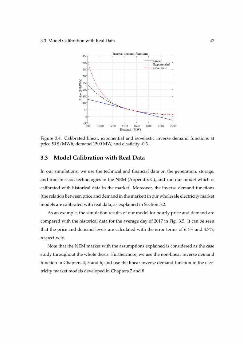
3.3 Model Calibration with Real Data 47
Demand (MW)800 1000 1200 1400 1600 1800 2000 2200
Pri
ce (
$/M
Wh)
-50
0
50
100
150
200
250
300
350
400
450Inverse demand functions
LinearExponentialIso-elastic
Figure 3.4: Calibrated linear, exponential and iso-elastic inverse demand functions atprice 50 $/MWh, demand 1500 MW, and elasticity -0.3.
3.3 Model Calibration with Real Data
In our simulations, we use the technical and financial data on the generation, storage,
and transmission technologies in the NEM (Appendix C), and run our model which is
calibrated with historical data in the market. Moreover, the inverse demand functions
(the relation between price and demand in the market) in our wholesale electricity market
models are calibrated with real data, as explained in Section 3.2.
As an example, the simulation results of our model for hourly price and demand are
compared with the historical data for the average day of 2017 in Fig. 3.5. It can be seen
that the price and demand levels are calculated with the error terms of 6.4% and 4.7%,
respectively.
Note that the NEM market with the assumptions explained is considered as the case
study throughout the whole thesis. Furthermore, we use the non-linear inverse demand
function in Chapters 4, 5 and 6, and use the linear inverse demand function in the elec-
tricity market models developed in Chapters 7 and 8.

48 NEM as the Case Study
1 6 121824
Pri
ce (
$/M
Wh)
50
100
150
200
250SA
hr1 6 121824
Dem
and (
MW
)
1000
1200
1400
1600
1800
2000
2200SA
1 6 1218240
100
200
300
400
500QLD
hr1 6 121824
4000
5000
6000
7000
8000
9000QLD
1 6 12182495
100
105
110
115
120
125TAS
hr1 6 121824
900
1000
1100
1200
1300TAS
1 6 12182460
80
100
120
140VIC
hr1 6 121824
3500
4000
4500
5000
5500
6000
6500VIC
1 6 12182450
100
150
200
250NSW
hr1 6 121824
6000
7000
8000
9000
10000
11000NSW
Figure 3.5: Comparing the simulation results (solid lines) of hourly price and demandwith the historical data (dashed lines) (Source: AEMO) for the average day of 2017 in
five states of the NEM.
Part II
Analysis of Price Volatility inElectricity Markets
49


Introduction to Part II 51
Introduction to Part II
AFTER introducing the Cournot-based electricity market models and embedding
storage firms in those models in Chapter 2, we extend the developed models and
apply them to analyze the price level and price volatility in electricity markets.
In Chapter 4, we develop a multi-region Cournot-based electricity market model
with non-linear inverse demand functions to find the impact of closing a base-load coal
power plant on electricity prices in Australia’s National Electricity Market. Calibrating
the model with real price and demand data and building wind power availability sce-
narios based on the historical daily wind data, we run the market model 365 times and
calculate the price volatility in NEM before and after closing down the coal power plant.
In Chapter 5, a bi-level optimization model is proposed to find the optimal storage
capacity at each node to limit the price volatility in the market to a target level. In the
upper level problem, the total storage capacity required to manage the price volatility is
minimized, and in the lower level problem, the interaction between strategic/regulated
generation, storage and transmission players is modeled using a stochastic (Bayesian)
Cournot-based game with exponential inverse demand functions.
In Chapter 6, a bi-level optimization model is proposed to allocate a fixed amount of
budget on wind and storage capacities to minimize the weighted sum of average price
and price volatility in the market. In the upper level problem, the weighted sum of price
and volatility is minimized by investing on battery and wind, and in the lower level
problem, the non-cooperative interaction between all market players is modeled using a
stochastic (Bayesian) Cournot-based game with exponential inverse demand functions.


Chapter 4
Impact of a Coal Power Plant Closureon a Multi-region Wholesale
Electricity Market
Closure of a base-load power plant, based on either its aging state, or a national greenhouse re-
duction scheme, or transition to smart grids, may have a significant impact on wholesale electricity
markets. This chapter presents a Cournot-based multi-region game model based on nonlinear inverse
demand functions to formally analyze the impacts of a base-load plant closure on the price level and
volatility (increase), and CO2 emission (decrease). Using the Hazelwood coal plant closure in Victo-
ria, a state of Australia’s National Electricity Market (NEM), as a case study, the simulation results
indicate around 30% and 49% price and volatility increase in the wholesale market, and 210 million
AU$ (+3.5%) higher annual power bills in Victoria for final consumers. However, being the most
stable and least volatile region in NEM, Victoria mostly supports its neighboring regions in terms of
price and volatility reduction even after the Hazelwood closure.
4.1 Introduction
IN THIS chapter, a game-theoretic multi-region electricity market model based on
nonlinear inverse demand functions is proposed. The model is used to analyze the
regional electricity prices after closure of a base-load coal-fueled generator in an electric-
ity market.
The contributions of this chapter are summarized as follows:
• A Mixed Complementarity Problem (MCP) is proposed to find the Nash Equi-
librium solution of a Cournot-based multi-region electricity market model with
53

54 Impact of a Coal Power Plant Closure on a Multi-region Wholesale Electricity Market
nonlinear inverse demand functions, including strategic generators (with market
power) and regulated transmission lines.
• We model the transmission lines as individual market participants likewise the
other players in the game and solve the model as an MCP problem, which is com-
putationally far more convenient than computing the electricity transmissions as
a constraint for market clearing engines in Equilibrium Problem with Equilibrium
Constraints (EPEC) electricity market models.
• The model is applied to the 5-node NEM market, as a case study, with realistic
data from year 2015. Our numerical results explain the actual real-life market data
events, e.g. price and demand, taking into account the market power of generation
firms. The simulation covers 365 days in a year and is calibrated with the real wind
generation and demand fluctuations.
• Lastly, the CO2 emission of gas and coal-fueled power plants, which is affected by
the electricity market price, is compared before and after the Hazelwood closure.
Under the proposed framework, we analyzed the impact of closing the Hazelwood
plant in Victoria on the regional electricity prices in NEM. The price level and price
volatility in different regions of NEM, the total profit the strategic generators make, and
the total CO2 emission are compared before and after the closure in our simulations. This
kind of study can inform the market players and system operator of the consequences
and ramifications of their decisions in advance.
The rest of this chapter is organized as follows. Section 4.2 illustrates the formulation
of the system model and the proposed MCP problem. Section 4.3 presents the simulation
results, and section 4.4 discusses the conclusion remarks.
4.2 System Model
We consider an electricity market consisting of I regions. Our market model includes
synchronous generators, wind firms, and transmission interconnectors. Let N sgi be the
set of synchronous generators, such as coal, gas, and hydro power plants, installed in
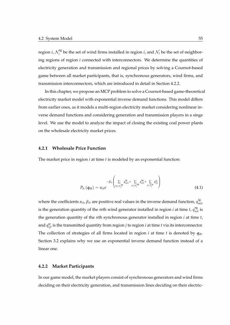
4.2 System Model 55
region i, N igi be the set of wind firms installed in region i, and Ni be the set of neighbor-
ing regions of region i connected with interconnectors. We determine the quantities of
electricity generation and transmission and regional prices by solving a Cournot-based
game between all market participants, that is, synchronous generators, wind firms, and
transmission interconnectors, which are introduced in detail in Section 4.2.2.
In this chapter, we propose an MCP problem to solve a Cournot-based game-theoretical
electricity market model with exponential inverse demand functions. This model differs
from earlier ones, as it models a multi-region electricity market considering nonlinear in-
verse demand functions and considering generation and transmission players in a singe
level. We use the model to analyze the impact of closing the existing coal power plants
on the wholesale electricity market prices.
4.2.1 Wholesale Price Function
The market price in region i at time t is modeled by an exponential function:
Pit (qit) = αite−βit
∑m∈N ig
i
qigmit+ ∑
n∈N sgi
qsgnit+ ∑
j∈N tri
qtrijt
(4.1)
where the coefficients αit, βit are positive real values in the inverse demand function, qigmit
is the generation quantity of the mth wind generator installed in region i at time t, qsgnit is
the generation quantity of the nth synchronous generator installed in region i at time t,
and qtrijt is the transmitted quantity from region j to region i at time t via its interconnector.
The collection of strategies of all firms located in region i at time t is denoted by qit.
Section 3.2 explains why we use an exponential inverse demand function instead of a
linear one.
4.2.2 Market Participants
In our game model, the market players consist of synchronous generators and wind firms
deciding on their electricity generation, and transmission lines deciding on their electric-

56 Impact of a Coal Power Plant Closure on a Multi-region Wholesale Electricity Market
ity exchange. In order to find its best response function, each market participant decides
on its decision variables, considering other players’ decision variables as an input, maxi-
mizing its objective function subject to the constraints corresponding to the technical and
operational limitations. The intersection of the best responses of all players is defined as
the Nash Equilibrium (NE) and solution of the game.
In our formulation, the wind firms and the synchronous generators are assumed to be
strategic, but the transmission firms are modeled as either strategic or regulated players.
Definition 4.1. A strategic (price maker) firm decides on its strategies over the operation horizon
1, ..., NT maximizing its aggregate profit over the operation horizon. On the other hand, a
regulated (price taker) firm aims to maximize the net market value, i.e. the social welfare [77].
Wind Generators
The best response of the mth wind (intermittent) generator in region i is obtained by
solving the following optimization problem:
maxqig
mit
t0
NT
∑t=1
Pit (qit) qigmit (4.2a)
s.t.
qigmit ≤ ωitQ
igmi ∀t (4.2b)
Pit (qit) ≤ Pcap ∀t (4.2c)
where qigmit is the generation level of the mth wind generator installed in region i at time t,
Qigmi is the capacity of the wind generator mi, ωit is the normalized wind power availabil-
ity coefficient of region i at time t, which represents the regional wind power availability
fluctuations, and Pcap represents the price cap in the market, which is, for example, 11000
$/MWh in Australian NEM. The constraint (4.2b) considers the wind energy availabil-
ity effect on power generation of the individual wind firm mi, and the constraint (4.2c)
secures the price cap in the market.

4.2 System Model 57
Synchronous Generators
The best response of the nth synchronous generator installed in region i is determined by
solving the following optimization problem:
maxqsg
nitt0
NT
∑t=1
(Pit (qit)− csg
ni
)qsg
nit (4.3a)
s.t.
qsgnit ≤ Qsg
ni ∀t (4.3b)
qsgnit − qsg
ni(t−1) ≤ Rupni ∀t (4.3c)
qsgni(t−1) − qsg
nit ≤ Rdnni ∀t (4.3d)
Pit (qit) ≤ Pcap ∀t (4.3e)
where qsgnit is the generation level of the nth synchronous generator installed in region
i at time t, Qsgni is the generation capacity of the synchronous generator ni, and csg
ni is its
marginal cost of generation. The constraint (4.3b) considers the generation capacity of the
synchronous generator ni, the constraints (4.3c) and (4.3d) ensure that the ramping limi-
tations of the synchronous generator ni are always met, and the constraint (4.3e) secures
the price cap in the market.
Transmission Firms
The best response of the transmission firm connecting the regions i and j is determined
by solving the following optimization problem:
maxqtr
jit,qtrijt
t
NT
∑t=1
(1− γtr
ij
) (Pjt(qjt)
qtrjit + Pit (qit) qtr
ijt
)+ γtr
ij
(Pjtw
(qjt)
−β jt+
Pitw (qit)
−βit
)(4.4a)
s.t.
qtrijt = −qtr
jit ∀t (4.4b)
−Qtrij ≤ qtr
ijt ≤ Qtrij ∀t (4.4c)

58 Impact of a Coal Power Plant Closure on a Multi-region Wholesale Electricity Market
Pkt (qkt) ≤ Pcap k ∈ i, j, ∀t (4.4d)
where qtrijt is the electricity exchange from region j to region i at time t, and Qtr
ij is the capac-
ity of the transmission line ij. The constraint (4.4b) ensures that the transmission levels
calculated on both directions of a line are identical, the constraint (4.4c) considers the
transmission capacity of the line ij, and the constraint (4.4d) secures the price cap in the
market. Note that the term Pjt(qjt)
qtrjit + Pit (qit) qtr
ijt is equal to(
Pit (qit)− Pjt(qjt))
qtrijt
which implies that the transmission firm may make profit by trading the electricity from
the node with lower price to the higher price node, and derivative of termPjtw(qjt)−β jt
+
Pitw(qit)−βit
with respect to qtrijt, given qtr
ijt = −qtrjit, is Pit (qit)− Pjt
(qjt)
which implies the firm
may trade electricity without market power. Therefore, when the coefficient γtrij is zero,
the transmission firm ij is modeled as a strategic player (profit maximizer), and when the
coefficient γtrij is one, the firm is modeled as a regulated player (social welfare maximizer).
Transmission firms or interconnectors are usually controlled by the market operator.
They are regulated to maximize the social welfare in the market. The existing litera-
ture discusses the markets with regulated transmission firms as electricity markets with
transmission constraint, e.g., see [7]. However, there are unregulated transmission firms
in some electricity markets, who make revenue by trading electricity across the regions
[78].
4.2.3 Solution Approach
Here, we seek for the intersection of the best response functions of all players in our
problem, i.e. the solution to the Karush-Kuhn-Tucker (KKT) conditions of all players.
The intersection of the best response functions of all players represents the NE solution.
The existence of a NE point in our problem is stated in Proposition 4.1.
Proposition 4.1. As the objective function of each player in our model is continuous and quasi-
concave in its strategy and their strategy space is compact, convex, and non-empty, our game
model admits a Nash Equilibrium solution.
Proof: The proof follows from Theorem 1.2 in [79].

4.3 Case Study and Simulation Results 59
Therefore, we look for a solution that satisfies the KKT conditions of wind generators,
(4.2a-4.2c), synchronous generators, (4.3a-4.3e), and transmission lines, (4.4a-4.4d). Note
that deriving the KKT conditions of the players’ optimization problems are discussed in
detail in [52]. The resulting MCP problem is as follows:
KKT (4.2a− 4.2c) , KKT (4.3a− 4.3e) , KKT (4.4a− 4.4d) :
m ∈ 1, ..., Nigi , n ∈ 1, ..., Nsg
i , i, j ∈ 1, ..., I
t ∈ 1, ..., NT
where the decision variables are the bidding strategies of all firms, and the set of La-
grange multipliers in KKT conditions. The problem is solved by PATH solver in GAMS
software.
4.3 Case Study and Simulation Results
In this section, we study the impact of closing a coal power plant on wholesale electricity
prices in market NEM.
4.3.1 Model Calibration
We simulated the NEM using a Cournot-based wholesale electricity market model with
exponential inverse demand functions. The coefficients of the inverse demand function
are calibrated with the real data of price and demand in five regions of NEM in 2015.
In order to verify the accuracy of our model in real market simulation, we compared
our simulation results for an average day splitted into 24 hours with the real historical
average price and demand data. The price and demand levels are calculated with the
error terms of 6.4% and 4.7% respectively. Then, we update the coefficients α and β in the
inverse demand functions for each day in all seasons, 365 days, based on the difference
of the historical price and demand at each day (scenario) from the average levels.

60 Impact of a Coal Power Plant Closure on a Multi-region Wholesale Electricity Market
4.3.2 Model Simulation for 365 Days
The stochastic parameters, such as intermittent power generation and demand variation,
are usually modeled by a set of scenarios in scenario-based electricity market models
[32, 33]. Scenario reduction techniques are applied to select any set of scenarios [80].
Instead of incorporating the scenario reduction simplifications, we capture the inter-
mittency and the price volatility existing in the market by repeating our simulations for
all 365 days in our model.
In order to observe the price fluctuations in different days during a year, we repeated
our simulation for all 365 days (24 hours) in year 2015, and captured the intermitten-
cies of wind power availability and demand variation in the model. Fig. 4.1 illustrates
the hourly variations of demand and wind power availability in 2015. The coefficients
αit and βit in the inverse demand function are calibrated with the historical price and
demand data enabling the model to follow the expected price and demand variations.
The normalized wind power availability coefficient wit is also calibrated based on the
historical hourly wind power generation in five regions of NEM during the year 2015.
We conducted our study to find the impact of closing the Hazelwood coal power
plant (1600 MW) in VIC on the electricity prices in different NEM’s regions. Table 4.1
indicates the regional average prices in NEM before and after the Hazelwood closure.
Our simulation results show that the average price of electricity goes up about 30.13% in
VIC and about 6.87% in total NEM after closing the plant Hazelwood, which shows more
price increase in the region in which closure happens. The electricity prices in QLD, the
region that is not directly connected to the region VIC, are almost unchanged after the
closure. Note that given the transmission and distribution cost of 120 $/MWh, the final
consumer prices in VIC goes up about 6.5% compared to the announced amount of 4%
in news (www.abc.net.au).
The electricity transmission direction between interconnected regions, to some extent,
indicates how a coal plant closure in one region affects the electricity prices in other re-
gions. As the region TAS behaves as a net importer of electricity from VIC before the
closure, the Hazelwood closure in VIC increases the prices in TAS notably. The region
SA is also a net importer of electricity from VIC, but the Hazelwood closure does not

4.3 Case Study and Simulation Results 61
0 2000 4000 6000 8000Demand
(MW)
020004000
SA
0 2000 4000 6000 8000
Wind
(MW)
010002000
SA
0 2000 4000 6000 8000Demand
(MW)
0500010000
QLD
0 2000 4000 6000 8000
Wind
(MW)
-101
QLD
0 2000 4000 6000 8000Demand
(MW)
010002000
TAS
0 2000 4000 6000 8000
Wind
(MW)
0200400
TAS
0 2000 4000 6000 8000Demand
(MW)
0500010000
VIC
0 2000 4000 6000 8000Wind
(MW)
05001000
VIC
hr(a)
0 2000 4000 6000 8000Demand
(MW) #104
0.511.5
NSW
hr(b)
0 2000 4000 6000 8000
Wind
(MW)
05001000
NSW
Figure 4.1: Sorted historical data of hourly (a) electricity demand and (b) wind poweravailability in five regions of NEM during the year 2015.
increase the average price in SA significantly due to the congestion of the interconnector
between SA and VIC.
Table 4.1: Wholesale electricity prices $/MWh in five-node NEM market, considering theclosure of coal power plant Hazelwood in VIC.
Price($/MWh)
SA QLD TAS VIC NSW NEM
Before closure 73.10 72.14 49.59 34.18 39.87 48.80After closure(change%)
75.06(2.67%)
72.16(0.02%)
53.80(8.50%)
44.48(30.12%)
40.21(0.86%)
52.16(6.87%)
The closure of Hazelwood power plant has different effects on electricity prices in dif-
ferent regions at different times. Fig. 4.2 indicates the probability distribution of hourly
electricity prices in the region VIC and in the total NEM. The probability distributions of
hourly prices in VIC and the total NEM indicate rightward shifts after the Hazelwood
closure. The price increment, i.e. rightward shift of the price probability distribution, is
more notable in VIC compared to the total NEM. The rate of average price increment in
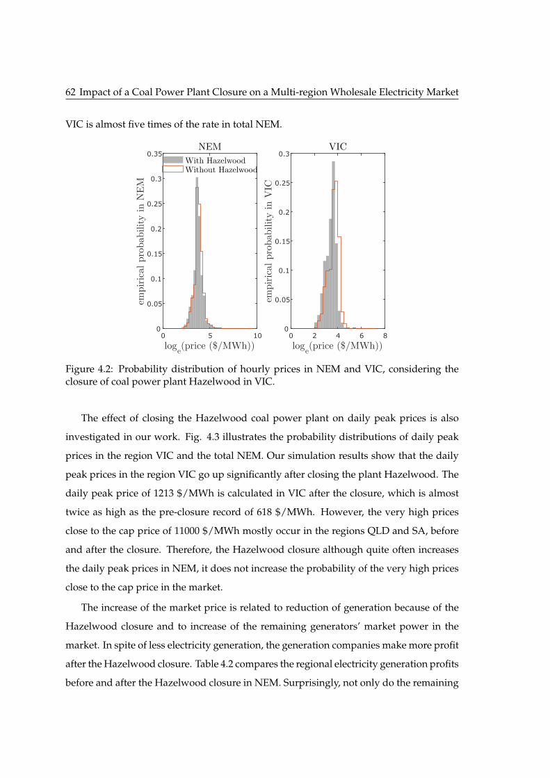
62 Impact of a Coal Power Plant Closure on a Multi-region Wholesale Electricity Market
VIC is almost five times of the rate in total NEM.
loge(price ($/MWh))
0 5 10
empir
ical
pro
bab
ility
in N
EM
0
0.05
0.1
0.15
0.2
0.25
0.3
0.35NEM
loge(price ($/MWh))
0 2 4 6 8
empir
ical
pro
bab
ility
in V
IC
0
0.05
0.1
0.15
0.2
0.25
0.3VIC
With HazelwoodWithout Hazelwood
Figure 4.2: Probability distribution of hourly prices in NEM and VIC, considering theclosure of coal power plant Hazelwood in VIC.
The effect of closing the Hazelwood coal power plant on daily peak prices is also
investigated in our work. Fig. 4.3 illustrates the probability distributions of daily peak
prices in the region VIC and the total NEM. Our simulation results show that the daily
peak prices in the region VIC go up significantly after closing the plant Hazelwood. The
daily peak price of 1213 $/MWh is calculated in VIC after the closure, which is almost
twice as high as the pre-closure record of 618 $/MWh. However, the very high prices
close to the cap price of 11000 $/MWh mostly occur in the regions QLD and SA, before
and after the closure. Therefore, the Hazelwood closure although quite often increases
the daily peak prices in NEM, it does not increase the probability of the very high prices
close to the cap price in the market.
The increase of the market price is related to reduction of generation because of the
Hazelwood closure and to increase of the remaining generators’ market power in the
market. In spite of less electricity generation, the generation companies make more profit
after the Hazelwood closure. Table 4.2 compares the regional electricity generation profits
before and after the Hazelwood closure in NEM. Surprisingly, not only do the remaining

4.3 Case Study and Simulation Results 63
loge(price ($/MWh))
2 4 6 8 10
empir
ical
pro
bab
ility
in N
EM
0
0.05
0.1
0.15
0.2
0.25NEM
loge(price ($/MWh))
2 4 6 8
empir
ical
pro
bab
ility
in V
IC0
0.05
0.1
0.15
0.2
0.25
0.3VIC
With HazelwoodWithout Hazelwood
Figure 4.3: Probability distribution of daily peak prices in NEM and VIC, considering theclosure of coal power plant Hazelwood in VIC.
generation companies make higher profits compared to their pre-closure profits, , but also
the total amount of generation profit, including the Hazelwood’s profit, is also higher
after the closure, as a result of market power increase after the Hazelwood closure.
Table 4.2: The annual electricity generation profit (billion$ per year) in five-node NEMmarket, considering the closure of coal power plant Hazelwood in VIC.
Profit(b$/year)
SA QLD TAS VIC NSW NEM
Before closure 0.38 1.55 0.32 1.33 1.08 4.68After closure(change%)
0.38(+2.2%)
1.55(+0.0%)
0.36(+9.9%)
1.54(+15.9%)
1.11(+2.9%)
4.96(+6.1%)
The standard deviation of electricity prices, consistent with
√∑
NTt=1(Pit−Pi)
2
NTwhere Pi is
the average price in region i, measures the price volatility and roughly indicates in which
regions very high electricity prices happen. Table 4.3 indicates the standard deviation
of electricity prices in different regions of the NEM. The state VIC although faces the
price volatility increment of 49% after the closure, it holds relatively low levels of price
standard deviation in the market NEM before and after the closure, which shows that VIC
is the most stable and least volatile region in NEM. In fact, before and after the closure,

64 Impact of a Coal Power Plant Closure on a Multi-region Wholesale Electricity Market
VIC mostly supports the other regions in terms of reducing their price level and price
volatility by exporting electricity via its interconnectors. It is observed that closing off
a power plant in VIC does not result in the unfavored very high prices close to the cap
price in NEM.
Table 4.3: Standard deviation of wholesale electricity prices $/MWh in five-node NEMmarket, considering the closure of coal power plant Hazelwood in VIC.
Deviation($/MWh)
SA QLD TAS VIC NSW NEM
Before closure 85.67 196.62 16.30 15.15 30.06 97.36After closure(change%)
85.57(-0.1%)
196.49(-0.07%)
16.70(+2.4%)
22.62(+49.2%)
29.90(-0.5%)
97.59(+0.2%)
Lastly, closure of the Hazelwood coal power plant in VIC changes the greenhouse
gas emission of CO2 from combustion of each fuel type, e.g. gas and coal, in the market
NEM. Table 4.4 compares the levels and changes of CO2 emission in NEM before and
after the closure of the plant Hazelwood. After the closure, the CO2 emission in NEM
reduces from coal combustion and increases from gas combustion. The decrease of coal-
fueled electricity generation after the plant closure results in higher electricity prices, and
consequently the more expensive gas-fueled electricity generation in the market becomes
more incentivized. In total, assuming the emission factor of 0.93 (tonneCO2 /MWh) for
coal and 0.55 (tonneCO2 /MWh) for gas, the aggregated CO2 emission in NEM from coal
and gas combustion decreases about 5.8% per year after closing the Hazelwood power
plant.
Table 4.4: Greenhouse gas emission of CO2 (million tonne per year) in coal and gas-fueledpower plants in NEM, considering the closure of coal power plant Hazelwood in VIC.
Emission(mtonne/year)
Coal Gas Total
Before closure 127 8.94 136After closure(change %)
118(-7.0%)
10.0(+11.8%)
128(-5.8%)

4.4 Conclusion 65
4.4 Conclusion
Closing down the base-load coal power plants, due to aging or intensive greenhouse
gas emission or growth of smart grids, is gradually taking place in many countries over
the world. Our study presents an MCP problem which solves a multi-region electricity
market game between wind firms, synchronous generators, and transmission lines before
and after closing a coal power plant in the market. Based on our numerical results, the
impact of closing the Hazelwood coal power plant in VIC on the electricity market NEM
can be summarized as:
• In a multi-region electricity market, coal power plant closure in one region may
affect the electricity prices in different regions. Closing the Hazelwood plant in
VIC has the highest impact on electricity prices in the region VIC and then on its
neighboring regions TAS and SA.
• The interconnectors also determine how a coal power plant closure may affect the
electricity prices in its neighboring regions. Both regions of SA and TAS are net
importers of electricity from VIC, but the price in SA does not change significantly
after the coal plant closure in VIC. The fact that the interconnector between SA and
VIC is usually congested prevents observing immense price changes in SA after the
Hazelwood closure.
• The region VIC faces a bounded price volatility increment inside its own region
after the Hazelwood closure. However, VIC, as the most stable and least volatile
region in NEM, continues to support its neighboring regions in terms of price level
and price volatility reduction even after the closure.
• The electricity generation companies enjoy higher amount of market power after
the Hazelwood closure, especially in VIC. Due to decrease of power generation
capacity in the market after the closure, generation companies may strategically
keep the prices higher and earn more profits.
• Although the closure of the Hazelwood coal plant increases the electricity prices in
NEM and incentivizes more gas fueled power generation and consequently leads

66 Impact of a Coal Power Plant Closure on a Multi-region Wholesale Electricity Market
to more emission from the gas generators, the aggregate effect of closing the Hazel-
wood plant down results in about 5.8% less CO2 emission from the coal and gas-
powered generators after the Hazelwood closure.
We observed in this chapter that closure of a coal power plant may increase the market
price and its volatility significantly. In Chapter 5, we study the integration of storage in
the network to find how it can help to reduce the high levels of electricity prices and price
volatility in the market.

Chapter 5
Impact of Optimal Storage Allocationon Price Volatility in Electricity
Markets
Recent studies show that the fast growing expansion of wind power generation may lead to ex-
tremely high levels of price volatility in wholesale electricity markets. Storage technologies, regardless
of their specific forms, e.g. pump-storage hydro, large-scale or distributed batteries, are capable of
alleviating the extreme price volatility levels due to their energy usage time shifting, fast-ramping
and price arbitrage capabilities. In this chapter, we propose a stochastic bi-level optimization model
to find the optimal nodal storage capacities required to achieve a certain price volatility level in a
highly volatile energy-only electricity market. The decision on storage capacities is made in the upper
level problem and the operation of strategic/regulated generation, storage and transmission players is
modeled in the lower level problem using an extended stochastic (Bayesian) Cournot-based game. The
South Australia (SA) electricity market, which has recently experienced high levels of price volatility,
and a 30-bus IEEE system are considered as the case studies. Our numerical results indicate that
50% price volatility reduction in SA electricity market can be achieved by installing either 430 MWh
regulated storage or 530 MWh strategic storage. In other words, regulated storage firms are more
efficient in reducing the price volatility than strategic storage firms.
5.1 Introduction
IN THIS chapter, a stochastic optimization framework is proposed for finding the
required nodal storage capacities in electricity markets with high levels of wind pen-
etration such that the price volatility in the market is kept below a certain level. Using
a proper storage allocation framework, the policy makers and market/system operators
can compute the required nodal storage capacities for managing the price volatility level
67

68 Impact of Optimal Storage Allocation on Price Volatility in Electricity Markets
in electricity markets. Although the current cost of storage systems is relatively high, the
support from governments (in the form of subsidies) and the eventual decline of the tech-
nology cost can lead to large scale integration of storage systems in electricity markets.
The contributions of this chapter are summarized as follows:
• A bi-level optimization model is proposed to find the optimal nodal storage capac-
ities required for avoiding the extreme price volatility levels in a nodal electricity
market.
• In the upper level problem, the total storage capacity is minimized subject to a price
volatility target constraint in each node and at each time.
• In the lower level problem, the non-cooperative interaction between generation,
transmission and storage players in the market is modeled as a stochastic (Bayesian)
Cournot-based game with an exponential inverse demand function. Note that the
equilibrium prices at the lower level problem are functions of the storage capacities.
The operation of storage devices at the lower level problem is modeled without
introducing binary variables.
• The existence of Bayesian Nash Equilibrium (Bayes-NE) [81] under the exponential
inverse demand function is established for the lower level problem.
Under the proposed framework, the size of storage devices at two nodes of South
Australia (SA) and Victoria (VIC) in NEM and also the size of storage in a 30-bus IEEE
system is determined such that the market price volatility is kept below a desired level at
all times. The desired level of price volatility can be determined based on various criteria
such as net revenue earned by the market players, occurrence frequency of undesirable
prices, number of CPT breaches, etc [82].
The rest of this chapter is organized as follows. The system model and the proposed
bi-level optimization problem are formulated in Section 5.2. The equilibrium analysis
of the lower level problem and the solution method are presented in Section 5.3. The
simulation results are presented in Section 5.4. The conclusion remarks are discussed in
Section 5.5.
5.2 System Model 69
5.2 System Model
Similar to the market model in Chapter 5, consider a nodal electricity market with I
nodes. Storage players are also included in our market model in this chapter. Let N sgi
be the set of synchronous generators, such as coal and gas power plants, located in node
i and N igi be the set of wind generation firms located in node i. The set of neighboring
nodes of node i is denoted by Ni. Since the wind availability is a stochastic parameter,
a scenario-based model, with Nw different scenarios, is considered to model the wind
availability in the electricity network. The nodal prices in our model are determined
by solving a stochastic (Bayesian) Cournot-based game among all market participants,
that is, synchronous generators, wind firms, storage firms and transmission interconnec-
tors which are introduced in detail in the lower level problem, given the wind power
availability scenarios. The decision variables, feasible region, and objective function for
each player in our game model are discussed in Section 5.2.2. In a Cournot game, each
producer (generator) competes for maximizing its profit which is defined as its revenue
minus its production cost, given the generation of other players. The revenue of each
player is its production level times the market price. Also, the market price is a func-
tion of total generation. Following the standard Cournot game models, any player in our
model maximizes its objective function given the decision variables of other players (gen-
eration, transmission, and storage firms). Considering different wind power availability
scenarios with given probabilities makes our game model consistent with the Bayesian
game definition. In a Bayesian game, players maximize their expected utility over a set
of scenarios with a given probability distribution [81].
In this chapter, we present a bi-level optimization approach for finding the minimum
required total storage capacity in the market such that the market price volatility stays
within a desired limit at each time.
5.2.1 Upper-level Problem
In the upper-level optimization problem, we determine the nodal storage capacities such
that a price volatility constraint is satisfied in each node at each time. In this chapter,

70 Impact of Optimal Storage Allocation on Price Volatility in Electricity Markets
estimates of variances are used to capture the volatilities [83], i.e., the variance of market
price is considered as a measure of price volatility. The variance of the market price in
node i at time t, i.e., Var(
Pitw), can be written as:
Var (Pitw) = Ew
[(Pitw (qitw))
2]− (Ew [P (qitw)])
2
= ∑w
(Pitw (qitw)
)2
Ψw −(
∑w
Pitw (qitw)Ψw
)2
(5.1)
where Ψw is the probability of scenario w, and Pitw (qitw) is the market price in node i at
time t under the wind availability scenario w, which is a function of the collection of all
players’ strategies qitw, i.e., the decision variables in the lower level game.
The notion of variance quantifies the effective variation range of random variables, i.e.
a random variable with a small variance has a smaller effective range of variation when
compared with a random variable with a large variance.
Given the price volatility relation (5.1) based on the Bayes-NE strategy collection of
all firms q?itw, the upper-level optimization problem is given by:
minQst
i i
I
∑i=1
Qsti
s.t.
Qsti ≥ 0 ∀i (5.2a)
Var (Pitw (q?itw)) ≤ σ2
0 ∀i, t (5.2b)
where Qsti is the storage capacity in node i, Pitw (q?
itw) is the market price in node i at
time t under the wind availability scenario w, and σ20 is the price volatility target. The
price volatility of the market is defined as the maximum variance of market price, i.e.
maxit Var(Pitw(q?itw)).

5.2 System Model 71
5.2.2 Lower-level Problem
In the lower-level problem, the nodal market prices and the Bayes-NE strategies of firms
are obtained by solving an extended stochastic Cournot-based game between wind gen-
erators, storage firms, transmission firms, and synchronous generators. Our model dif-
fers from a standard Cournot game, such that it includes regulated players in addition to
strategic players in generation, storage and transmission levels.
Definition 5.1. A strategic (price maker) firm decides on its strategies over the operation horizon
1, ..., NT such that its aggregate expected profit, over the operation horizon, is maximized. On
the other hand, a regulated (price taker) firm aims to maximize the net market value, i.e. the social
welfare [77].
The market price in node i at time t under the wind availability scenario w is given
by an exponential inverse demand function (Section 3.2):
Pitw (qitw) = αite−βit
qstitw+ ∑
m∈N igi
qigmitw+ ∑
n∈N sgi
qsgnitw+ ∑
j∈Ni
qtrijtw
(5.3)
where αit, βit are positive real values in the inverse demand function, qsgnitw is the genera-
tion strategy of the nth synchronous generator located in node i at time t under scenario
w, qigmitw is the generation strategy of the mth wind generator located in node i at time t
under scenario w, qstitw is the charge/discharge strategy of the storage firm in node i at
time t under scenario w, qtrijtw is the strategy of transmission firm located between node
i and node j at time t under scenario w. The collection of strategies of all firms located
in node i at time t under the scenario w is denoted by qitw. Note that the total amount
of power supply from the generation and storage firms plus the net import/export, i.e.,
qstitw + ∑
m∈N igi
qigmitw + ∑
n∈N sgi
qsgnitw + ∑
j∈Ni
qtrijtw, is equal to the net electricity demand in each
node, at each time and under each scenario, which represents the nodal electricity balance
in our model.
In what follows, the variable µ is used to indicate the associated Lagrange variable
with its corresponding constraint in the model.

72 Impact of Optimal Storage Allocation on Price Volatility in Electricity Markets
Wind Generators
The Bayes-NE strategy of the mth wind (intermittent) generator in node i is obtained by
solving the following optimization problem:
maxqig
mitw
tw0
∑w
Ψw
NT
∑t=1
Pitw (qitw) qigmitw
(1− γ
igmi
)+ γ
igmi
(Pitw (qitw)
−βit
)
s.t.
qigmitw ≤ Qig
mitw : µig,maxmitw ∀t, w (5.4a)
Pitw (qitw) ≤ Pcap : µig,capmitw ∀t, w (5.4b)
where qigmitw and Qig
mitw are the generation level and the available wind capacity of the
mth wind generator located in node i at time t under scenario w. The parameter Pcap
represents the price cap in the market, which is, for instance, 11000 $/MWh in the NEM
market. Setting cap price in electricity markets also aims to limit the price levels and price
volatility levels. Note that the wind availability changes in time in a stochastic manner,
and the wind firm’s bids depend on the wind availability. As a result, the nodal prices
and decisions of the other firms become stochastic in our model [33].
The mth wind firm in node i acts as a strategic firm in the market if γigmi is equal to
zero and acts as a regulated firm if γigmi is equal to one. The difference between regulated
and strategic players corresponds to the strategic price impacting capability. In fact, a
regulated firm behaves as a price taker player while a strategic firm behaves as a price
maker player.
Storage Firms
Storage firms benefit from price difference at different times to make profit, i.e. they
sell the off-peak stored electricity at higher prices at peak times. The Bayes-NE strategy
of storage firm located in node i is determined by solving the following optimization

5.2 System Model 73
problem:
maxqdis
itw,qchitwtw
0
,qstitwtw
∑w
Ψw
NT
∑t=1
Pitw (qitw) qstitw(1− γst
i)− cst
i
(qdis
itw + qchitw
)+ γst
i
(Pitw (qitw)
−βit
)
s.t.
qstitw = ηdis
i qdisitw −
qchitw
ηchi
: µstitw ∀t, w (5.5a)
qdisitw ≤ ζdis
i Qsti : µdis,max
itw ∀t, w (5.5b)
qchitw ≤ ζch
i Qsti : µch,max
itw ∀t, w (5.5c)
0 ≤t
∑t′=1
(qch
it′w − qdisit′w
)∆ ≤ Qst
i : µst,minitw , µst,max
itw ∀t, w (5.5d)
Pitw (qitw) ≤ Pcap : µst,capitw ∀t, w (5.5e)
where qdisitw and qch
itw are the discharge and charge levels of the storage firm in node i at time
t under scenario w, respectively, csti is the unit operation cost, ηch
i ,ηdisi are the charging and
discharging efficiencies, respectively, and qstitw is the net supply/demand of the storage
firm in node i. The parameter ζchi (ζdis
i ) is the percentage of storage capacity Qsti , which
can be charged (discharged) during time period ∆. It is assumed that the storage devices
are initially fully discharged. The energy level of the storage device in node i at each time
is limited by its capacity Qsti . Note that the nodal market prices depend on the storage
capacities, i.e. Qsti s, through the constraints (5.5b)-(5.5d). This dependency allows the
market operator to meet the volatility constraint using the optimal values of the storage
capacities. The storage capacity variables are the only variables that couple the scenarios
in the lower level problem. Therefore, each scenario of the lower lever problem can be
solved separately for any storage capacity amount. The storage firm in node i acts as a
strategic firm in the market if γsti is equal to zero and acts as a regulated firm if γst
i is equal
to one.
Proposition 5.1. At the Bayes-NE of the lower level game, each storage firm is either in the
charge mode or discharge mode at each scenario, i.e. the charge and discharge levels of each storage
firm cannot be simultaneously positive at the NE of each scenario.

74 Impact of Optimal Storage Allocation on Price Volatility in Electricity Markets
Proof: See Appendix A.
Synchronous Generators
Synchronous generators include coal, gas, hydro and nuclear power plants. The Bayes-
NE strategy of nth synchronous generator located in node i is determined by solving the
following optimization problem:
maxqsg
nitwtw0
∑w
Ψw
NT
∑t=1
Pitw (qitw) qsgnitw
(1− γ
sgni
)− csg
ni qsgnitw + γ
sgni
(Pitw (qitw)
−βit
)s.t.
qsgnitw ≤ Qsg
ni : µsg,maxnitw ∀t, w (5.6a)
qsgnitw − qsg
ni(t−1)w ≤ Rupni Qsg
ni : µsg,upnitw ∀t, w (5.6b)
qsgni(t−1)w − qsg
nitw ≤ Rdnni Qsg
ni : µsg,dnnitw ∀t, w (5.6c)
Pitw (qitw) ≤ Pcap : µsg,capnitw ∀t, w (5.6d)
where qsgnitw is the generation level of the nth synchronous generator in node i at time t
under scenario w, Qsgni and csg
ni are the capacity and the short term marginal cost of the nth
synchronous generator in node i, respectively. The constraints (5.6b) and (5.6c) ensure
that the ramping limitations of the nth synchronous generator in node i are always met.
The nth synchronous generator in node i acts as a strategic firm in the market if γsgni is
equal to zero and acts as a regulated firm if γsgni is equal to one.
Transmission Firms
The Bayes-NE strategy of the transmission firm between nodes i and j is determined by
solving the following optimization problem:
maxqtr
jitw,qtrijtw
tw
∑w
Ψw
NT
∑t=1
(1− γtr
ij
) (Pjtw
(qjtw
)qtr
jitw + Pitw (qitw) qtrijtw
)

5.3 Solution Approach 75
+ γtrij
Pjtw
(qjtw
)−β jt
+Pitw (qitw)
−βit
s.t.
qtrijtw = −qtr
jitw : µtrijtw ∀t, w (5.7a)
−Qtrij ≤ qtr
ijtw ≤ Qtrij : µtr,min
ijtw , µtr,maxijtw ∀t, w (5.7b)
Pktw (qktw) ≤ Pcap : µtr,capkk′tw k, k′ ∈ i, j, k 6= k′ ∀t, w (5.7c)
where qtrijtw is the electricity flow from nodes j to i at time t under scenario w, and Qtr
ij is
the capacity of the transmission line between node i and node j. The transmission firm
between nodes i and j behaves as a strategic player when γtrij is equal to zero and behaves
as a regulated player when γtrij is equal to one. Note that the term Pjtw
(qjtw
)qtr
jitw +
Pitw (qitw) qtrijtw in the objective function of the transmission firm is equal to (Pjtw
(qjtw
)−
Pitw (qitw))qtrjitw which implies that the transmission firm between two nodes makes profit
by transmitting electricity from the node with lower market price to the node with higher
market price. Moreover, the price difference between the paired nodes indicates the con-
gestion on the transmission lines and can be used to set the value of Financial Transmis-
sion Rights (FTR) [84] in electricity markets.
Transmission lines or interconnectors are usually controlled by the market opera-
tor and are regulated to maximize the social welfare in the market. The markets with
regulated transmission firms are discussed as electricity markets with transmission con-
straints in the literature, e.g., see [20,31,35]. However, some electricity markets allow the
transmission lines to act strategically, i.e. to make revenue by trading electricity across
the nodes [78].
5.3 Solution Approach
In this section, we first provide a game-theoretic analysis of the lower-level problem.
Next, the bi-level price volatility management problem is transformed to a single opti-
mization Mathematical Problem with Equilibrium Constraints (MPEC).

76 Impact of Optimal Storage Allocation on Price Volatility in Electricity Markets
5.3.1 Game-theoretic Analysis of the Lower-level Problem
To solve the lower-level problem, we need to study the best response functions of firms
participating in the market. Then, any intersection of the best response functions of all
firms in all scenarios will be a Bayes-NE. In this subsection, we first establish the existence
of Bayes-NE for the lower-level problem. Then, we provide the necessary and sufficient
conditions which can be used to solve the lower-level problem.
To transform the bi-level price volatility management problem to a single level prob-
lem, we need to ensure that for every vector of storage capacities, i.e. Qst = [Qst1 , · · · , Qst
I ]> ≥
0, the lower-level problem admits a Bayes-NE. At the Bayes-NE strategy of the lower-
level problem, no single firm has any incentive to unilaterally deviate its strategy from
its Bayes-NE strategy. Note that the objective function of each firm is quasi-concave in its
strategy and constraint set of each firm is closed and bounded for all Qst = [Qst1 , · · · , Qst
I ]> ≥
0. Thus, the lower level game admits a Bayes-NE. This result is formally stated in Propo-
sition 5.2.
Proposition 5.2. For any vector of storage capacities, Qst = [Qst1 , · · · , Qst
I ]> ≥ 0, the lower
level game admits a Bayes-NE.
Proof: Note that the objective function of each firm is continuous and quasi-concave
in its strategy. Also, the strategy space is non-empty, compact and convex. Therefore, ac-
cording to Theorem 1.2 in [79], the lower level game admits a Bayes-NE.
Best responses of wind firm mi
Let q−(mi) be the strategies of all firms in the market except the wind generator m located
in node i. Then, the best response of the wind generator m in node i to q−(mi) satisfies
the necessary and sufficient Karush-Kuhn-Tucker (KKT) conditions (t ∈ 1, ..., NT; w ∈
1, ..., Nw):
Pitw (qitw) + (1− γigmi)
∂Pitw (qitw)
∂qigmitw
qigmitw −
µig,maxmitw +
∂Pitw(qitw)
∂qigmitw
µig,capmitw
Ψw≤ 0 ⊥ qig
mitw ≥ 0
(5.8a)

5.3 Solution Approach 77
qigmitw ≤ Qig
mitw ⊥ µig,maxmitw ≥ 0 (5.8b)
Pitw (qitw) ≤ Pcap ⊥ µig,capitw ≥ 0 (5.8c)
where the perpendicularity sign, ⊥, means that at least one of the adjacent inequalities
must be satisfied as an equality [73].
Best responses of storage firm i
To study the best response of the storage firm in node i, let q−i denote the collection
of strategies of all firms except the storage firm in node i. Then, the best response of
the storage firm in node i is obtained by solving the following KKT conditions (t ∈
1, ..., NT; w ∈ 1, ..., Nw):
Pitw (qitw) + (1− γsti )
∂Pitw (qitw)
∂qstitw
qstitw +
µstitw −
∂Pitw(qitw)∂qst
itwµ
st,capitw
Ψw= 0 (5.9a)
−ηdisi µst
itw − µdis,maxitw − ∆ ∑NT
t′=t
(µst,min
it′w − µst,maxit′w
)Ψw
− csti ≤ 0 ⊥ qdis
itw ≥ 0 (5.9b)
µstitw
ηchi− µch,max
itw + ∆ ∑NTt′=t
(µst,min
it′w − µst,maxit′w
)Ψw
− csti ≤ 0 ⊥ qch
itw ≥ 0 (5.9c)
qstitw = ηdis
i qdisitw −
qchitw
ηchi
(5.9d)
qdisitw ≤ ζdis
i Qsti ⊥ µdis,max
itw ≥ 0 (5.9e)
qchitw ≤ ζch
i Qsti ⊥ µch,max
itw ≥ 0 (5.9f)
0 ≤t
∑t′=1
(qch
it′w − qdisit′w
)∆ ⊥ µst,min
itw ≥ 0 (5.9g)
t
∑t′=1
(qch
it′w − qdisit′w
)∆ ≤ Qst
i ⊥ µs,maxitw ≥ 0 (5.9h)
Pitw (qitw) ≤ Pcap ⊥ µst,capitw ≥ 0 (5.9i)

78 Impact of Optimal Storage Allocation on Price Volatility in Electricity Markets
Best responses of synchronous generation firm ni
The best response of the synchronous generator n in node i to q−(ni), i.e. the collection of
strategies of all firms except the synchronous generator n in node i, is obtained by solving
the following KKT conditions (t ∈ 1, ..., NT; w ∈ 1, ..., Nw):
Pitw (qitw)− csgni + (1− γ
sgni )
∂Pitw (qitw)
∂qsgnitw
qsgnitw −
µsg,maxnitw +
∂Pitw(qitw)
∂qsgnitw
µsg,capnitw
Ψw
+µ
sg,upni(t+1)w − µ
sg,upnitw + µ
sg,dnnitw − µ
sg,dnni(t+1)w
Ψw≤ 0 ⊥ qsg
nitw ≥ 0 (5.10a)
qsgnitw ≤ Qsg
ni ⊥ µsg,maxnitw (5.10b)
qsgnitw − qsg
ni(t−1)w ≤ Rupni Qsg
ni ⊥ µsg,upnitw ≥ 0 (5.10c)
qsgni(t−1)w − qsg
nitw ≤ Rdnni Qsg
ni ⊥ µsg,dnnitw ≥ 0 (5.10d)
Pitw (qitw) ≤ Pcap ⊥ µsg,capnitw ≥ 0 (5.10e)
Best responses of transmission firm ij
Finally, the best response of the transmission firm between nodes i and j, to q−(ij), i.e. the
set of all firms’ strategies except those of the transmission line between nodes i and j, can
be obtained using the KKT conditions (t ∈ 1, ..., NT; w ∈ 1, ..., Nw):
Pitw (qitw) +(
1− γtrij
) ∂Pitw (qitw)
∂qtrijtw
qtrijtw +
µtrjitw+µtr
ijtw+µtr,minijtw −µtr,max
ijtw − ∂Pitw(qitw)∂qtr
ijtwµ
tr,capijtw
Ψw= 0
(5.11a)
qtrijtw = −qtr
jitw (5.11b)
−Qtrij ≤ qtr
ijtw ⊥ µtr,minijtw ≥ 0 (5.11c)
qtrijtw ≤ Qtr
ij ⊥ µtr,maxijtw ≥ 0 (5.11d)
Pitw (qitw) ≤ Pcap ⊥ µtr,capijtw ≥ 0 (5.11e)

5.3 Solution Approach 79
5.3.2 The Equivalent Single-level Problem
Here, the bi-level price volatility management problem is transformed into a single-level
MPEC. To this end, note that for every vector of storage capacities the market price can be
obtained by solving the firms’ KKT conditions. Thus, by imposing the KKT conditions of
all firms as constraints in the optimization problem (5.2), the price volatility management
problem can be written as the following single-level optimization problem:
minI
∑i=1
Qsti (5.12)
s.t.
(5.2a− 5.2b), (5.8a− 5.8c), (5.9a− 5.9i), (5.10a− 5.10e), (5.11a− 5.11e)
m ∈ 1, ..., Nigi , n ∈ 1, ..., Nsg
i , i, j ∈ 1, ..., I,
t ∈ 1, ..., NT; w ∈ 1, ..., Nw
where the optimization variables are the storage capacities, the bidding strategies of all
firms and the set of all Lagrange multipliers. Because of the nonlinear complementary
constraints, the feasible region is not necessarily convex or even connected. Therefore,
increasing the storage capacities stepwise, ∆Qst, we solve the lower level problem, which
is convex.
Remark: It is possible to convert the equivalent single level problem (5.12) to a Mixed-
Integer Non-Linear Problem (MINLP). However, the large number of integer variables
potentially makes the resulting MINLP computationally infeasible.
The MPEC problem (5.12) can be solved using extensive search when the number of
nodes is small. For large electricity networks, the greedy algorithm proposed in [85] can
be used to find the storage capacities iteratively while the other variables are calculated
as the solution of the lower level problem. In each iteration, the lower level problem is
solved as a Mixed Complementarity Problem (MCP) [86], which is sometimes termed
as rectangular variational inequalities. The optimization solution method is illustrated
in Algorithm 1. The storage capacity variable is discretized and the increment storage
capacity of ∆Qst is added to the selected node i∗ at each iteration of the algorithm. Once

80 Impact of Optimal Storage Allocation on Price Volatility in Electricity Markets
the price volatility constraint is satisfied with equality, the optimum solution is found.
Although our greedy algorithm just guarantees a locally optimal storage capacity, we
obtained the same results in NEM market using the extensive search.
Algorithm 1 The greedy algorithm for finding the storage allocation
while maxit Var(Pitw(q?itw)) > σ2
0 doiteration=iteration+1for i′ = 1 : I do
Qsti′ (iteration)← Qst
i′ (iteration− 1) +4Qst
Qst−i′(iteration)← Qst
−i′(iteration− 1)q? ← Lower level problem Bayes−NEPrice Volatility(i′)← maxit Var(Pitw(q?
itw))end fori∗ ← find
i(min(Price Volatility(i)))
Qsti∗(iteration)← Qst
i∗(iteration− 1) +4Qst
end while
5.4 Case Study and Simulation Results
In this section, we apply our price volatility management framework to two different
types of electricity markets: (i) the NEM market, which has a regional pricing mechanism,
(ii) a 30-bus electricity system with a Locational Marginal Pricing (LMP) mechanism [87].
The most important difference between LMP and regional pricing markets is the number
of settlement prices. Tens or hundreds of pricing nodes may be required to implement
a LMP market whereas in a regional pricing only few settlement prices are considered.
Note that the optimization problem (5.12) can model both regional and LMP markets.
5.4.1 Simulations in NEM
In this subsection, we study the impact of storage installation on price volatility in two
nodes of Australia’s National Electricity Market (NEM), South Australia (SA) and Vic-
toria (VIC), with regional pricing mechanism, which sets the marginal value of demand
at each region as the regional prices. SA has a high level of wind penetration and VIC
has high coal-fueled synchronous generation. Real data for price and demand from the

5.4 Case Study and Simulation Results 81
year 2015 is used to calibrate the inverse demand function in the model. Different types
of generation firms, such as coal, gas, hydro, wind and biomass, with generation ca-
pacity (intermittent and dispatchable) of 3.7 GW and 11.3 GW were active in SA and
VIC, respectively, in 2015. The transmission line interconnecting SA and VIC, which is
a regulated line, has the capacity of 680 MW but currently is working with just 70% of
its capacity. The generation capacities in our numerical results are gathered from Aus-
tralian Electricity Market Operator’s (AEMO’s) website (aemo.com.au) and all the prices
are shown in Australian dollar.
In our study, we consider a set of scenarios each representing a 24-hour wind power
availability profile. In order to guarantee a high level of accuracy, we do not employ
scenario reduction methods [80] and instead consider 365 daily wind power availability
scenarios, with equal probabilities, using the realistic data from the year 2015 in different
regions of NEM (source of data: AEMO). Fig. 5.1 shows the hourly wind power avail-
ability in SA. On each box in Fig. 5.1, the central mark indicates the average level and the
bottom and top edges of the box indicate the 25th and 75th percentiles of wind power
availability from the 365 scenarios, respectively. It can be seen that in SA the wind power
capacity is about 1200 MW and the wind capacity factor is about 33-42% at different
hours.
In what follows, by price volatility we mean the maximum variance of market price,
i.e. maxit Var(Pitw(q?itw)). Also, by square root of price volatility we mean the maximum
standard deviation of market price, i.e. maxit
√Var(Pitw(q?
itw).
One-region model simulations in South Australia
In our one-region model simulations, we first study the impacts of peak demand levels
and supply capacity shortage on the standard deviation of hourly electricity prices (or
square root of hourly price volatilities) in SA with no storage. Next, we study the effect
of storage on the price volatility in SA. Fig. 5.2 shows the average and standard deviation
of hourly prices for a day in SA (with no storage) for three different cases: (i) a regular
demand day, (ii) a high demand day, (iii) a high demand day with coal-plant outage.

82 Impact of Optimal Storage Allocation on Price Volatility in Electricity Markets
hr1 2 3 4 5 6 7 8 9 101112131415161718192021222324
Win
d P
ower
(M
W)
0
200
400
600
800
1000
1200
Hourly wind power availability distribution in SA
Figure 5.1: SA’s Hourly wind power availability distribution in 2015 (the central marksshow the average levels and the bottom and top edges of the boxes indicate the 25th and75th percentiles).
An additional load of 1000 MW is considered in the high demand case during hours 16,
17 and 18 to study the joint effect of wind intermittency and large demand variations
on the price volatility. The additional loads are sometimes demanded in the market due
to unexpected high temperatures happening in the region. The coal-plant outage case
is motivated by the recent retirement of two coal-plants in SA with total capacity of 770
MW [88]. This allows us to investigate the joint impact of wind indeterminacy and low
base-load generation capacity on the price volatility.
According to Fig. 5.2, wind power fluctuation does not create much price fluctuation
in a regular demand day. The square root of the price volatility in the regular demand
day is equal to 65 $/MWh. Depending on the wind power availability level, the peak
price varies from 92 $/MWh to 323 $/MWh, with average of 210 $/MWh, in a regular
demand day. Based on Fig. 5.2, the square root of the price volatility in the high demand
day is equal to 1167 $/MWh. The maximum price in a high demand day in SA changes
from 237 $/MWh to 4466 $/MWh, with average of 1555 $/MWh, because of wind power
availability fluctuation. The extra load at peak times and the wind power fluctuation cre-
ate a higher level of price volatility during a high demand day compared with a regular

5.4 Case Study and Simulation Results 83
demand day.
The retirement (outage) of coal-plants in SA beside the extra load at peak hours in-
creases the price volatility due to the wind power fluctuation. The maximum price dur-
ing the high demand day with coal-plant outage varies from 377 $/MWh to the cap price
of 11000 $/MWh, with average of 5832 $/MWh. The square root of the price volatility
during the high demand day with coal-plant outage is equal to 4365 $/MWh. The square
root of the price volatility during the high demand day with coal-plant outage is almost
67 times more than the regular demand day due to the simultaneous variation in both
supply and demand.
2 4 6 8 10 12 14 16 18 20 22 24
$/M
Wh
0
200
400
(i) Mean and standard deviation of hourly prices ina regular demand day
Standard deviationMean
2 4 6 8 10 12 14 16 18 20 22 24
$/M
Wh
0
1000
2000
(ii) Mean and standard deviation of hourly prices ina high demand day
hr2 4 6 8 10 12 14 16 18 20 22 24
$/M
Wh
0
5000
10000
(iii) Mean and standard deviation of hourly prices ina high demand day with coal-plants outage
Figure 5.2: Standard deviation and mean of hourly wholesale electricity prices in SA withno storage.
Fig. 5.3 shows the minimum required (strategic/regulated) storage capacities for
achieving various levels of price volatility in SA during a high demand day with coal-
plant outage. The minimum storage capacities are calculated by solving the optimization
problem (5.12) for the high demand day with coal-plant outage case. According to Fig.
5.3, a strategic storage firm requires a substantially larger capacity, compared with a reg-
ulated storage firm, to achieve a target price volatility level due to the selfish behavior
of the storage firms. In fact, the strategic storage firms may sometimes withhold their

84 Impact of Optimal Storage Allocation on Price Volatility in Electricity Markets
available capacities and do not participate in the price volatility reduction as they do not
always benefit from reducing the price. The price volatility in SA can be reduced by 50%
using either 530 MWh strategic storage or 430 MWh regulated storage. Note that AEMO
has forecasted about 500 MWh battery storage to be installed in SA until 2035 [89].
Percentage of price volatility reduction10% 20% 30% 40% 50%
Opti
mal
sto
rage
cap
acity
(MW
h)
0
50
100
150
200
250
300
350
400
450
500
550Optimal storage capacity for price volatility reduction
Strategic storageRegulated storage
Figure 5.3: Optimal strategic and regulated storage capacity for achieving different pricevolatility levels in SA region for a high demand day with coal-plant outage.
According to our numerical results, storage can displace the peaking generators, with
high fuel costs and market power, which results in reducing the price level and the
price volatility. A storage capacity of 500 MWh (or 500 MW given the discharge coef-
ficient ηdis = 1) reduces the square root of the price volatility from 4365 $/MWh to 2692
$/MWh, almost 38% reduction, during a high demand day with coal-plant outage in SA.
The behaviour of the peak and the daily average prices for the high demand day with
coal-plant outage in SA is illustrated in Fig. 5.4. In this figure, the peak price represents
the average of highest prices over all scenarios during the day, i.e. ∑w Ψw (maxt Ptw(q?tw))
and the daily average price indicates the average of price over time and scenarios, i.e.1
NT∑tw Ptw(q?tw)Ψw. Sensitivity analysis of the peak and the daily average prices in SA
with respect to storage capacity indicates that high storage capacities lead to relatively
low prices in the market. At very high prices, demand is almost inelastic and a small

5.4 Case Study and Simulation Results 85
amount of excess supply leads to a large amount of price reduction. According to Fig.
5.4, the rate of peak price reduction decreases as the storage capacity increases since large
storage capacities lead to lower peak prices which make the demand more elastic.
Based on Fig. 5.4, the impact of storage on the daily average and peak prices de-
pends on whether the storage firm is strategic or regulated. It can be observed that the
impacts of strategic and regulated storage firms on the daily peak/average prices are al-
most similar for small storage capacities, i.e. when the storage capacity is smaller than
100 MWh (or 100 MW given ηdis = 1). However, a regulated firm reduces both the peak
and the average prices more efficiently compared with a strategic storage firm as its ca-
pacity becomes large. A large strategic storage firm in SA does not use its excess capacity
beyond 500 MWh to reduce the market price since it acts as a strategic profit maximizer,
but a regulated storage firm contributes to the price volatility reduction as long as there
is potential for price reduction by its operation.
Storage capacity (MWh)0 200 400 600
Pri
ce (
$/M
Wh)
350
400
450
500
550
600
650
700
750
800
Daily average priceversus storage capacity
Storage capacity (MWh)0 200 400 600
2000
2500
3000
3500
4000
4500
5000
5500
6000
6500
Peak priceversus storage capacity
Regulated storageStrategic storage
Figure 5.4: Daily peak and average prices in SA versus storage capacity in a high demandday with coal-plant outage.
Fig. 5.5 depicts the square root of price volatility versus storage capacity in SA during
the high demand day with coal-plant outage. According to this figure, the price volatility
in the market decreases by installing either regulated or strategic storage devices. To
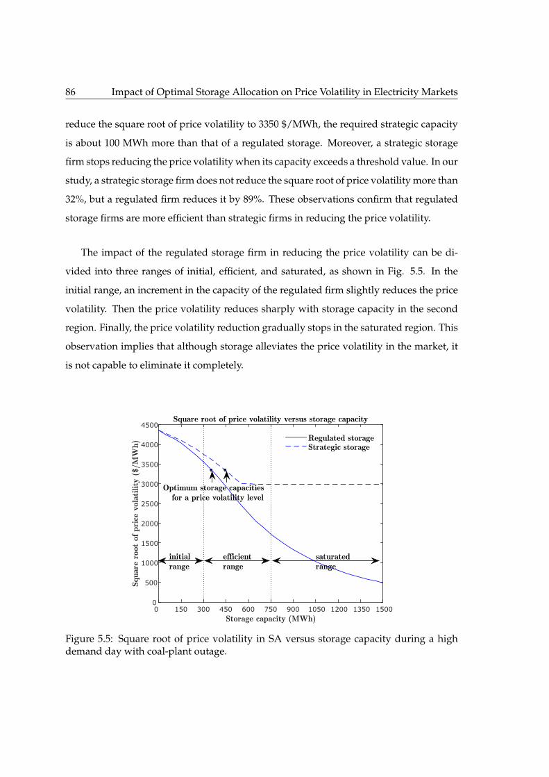
86 Impact of Optimal Storage Allocation on Price Volatility in Electricity Markets
reduce the square root of price volatility to 3350 $/MWh, the required strategic capacity
is about 100 MWh more than that of a regulated storage. Moreover, a strategic storage
firm stops reducing the price volatility when its capacity exceeds a threshold value. In our
study, a strategic storage firm does not reduce the square root of price volatility more than
32%, but a regulated firm reduces it by 89%. These observations confirm that regulated
storage firms are more efficient than strategic firms in reducing the price volatility.
The impact of the regulated storage firm in reducing the price volatility can be di-
vided into three ranges of initial, efficient, and saturated, as shown in Fig. 5.5. In the
initial range, an increment in the capacity of the regulated firm slightly reduces the price
volatility. Then the price volatility reduces sharply with storage capacity in the second
region. Finally, the price volatility reduction gradually stops in the saturated region. This
observation implies that although storage alleviates the price volatility in the market, it
is not capable to eliminate it completely.
Storage capacity (MWh)0 150 300 450 600 750 900 1050 1200 1350 1500
Squ
are
root
of pri
ce v
olat
ility
($/M
Wh)
0
500
1000
1500
2000
2500
3000
3500
4000
4500
initialrange
efficientrange
saturatedrange
Square root of price volatility versus storage capacity
Regulated storageStrategic storage
Optimum storage capacitiesfor a price volatility level
Figure 5.5: Square root of price volatility in SA versus storage capacity during a highdemand day with coal-plant outage.

5.4 Case Study and Simulation Results 87
Two-region model simulations in South Australia and Victoria
In the one-region model simulations, we analysed the impact of storage on the price
volatility in SA when the SA-VIC interconnector is not active. In this subsection, we first
study the effect of the interconnector between SA and VIC on the price volatility in the
absence of storage firms. Next, we investigate the impact of storage firms on the price
volatility when the SA-VIC transmission line operates at various capacities. In our nu-
merical results, SA is connected to VIC using a 680 MW interconnector which is currently
operating with 70% of its capacity, i.e. 30% of its capacity is under maintenance. The nu-
merical results in this subsection are based on the two-node model for a high demand
day with coal-plant outage in SA. To investigate the impact of transmission line on price
volatility, it is assumed that the SA-VIC interconnector operates with 60% and 70% of its
capacity.
According to our numerical results, the peak price (the average of highest prices over
all scenarios) in SA is equal to 6154 $/MWh when the SA-VIC interconnector is com-
pletely in outage. However, the peak price reduces to 3328 $/MWh and 2432 $/MWh
when the interconnector operates at 60% and 70% of its capacity. The square root of price
volatility is 4365 $/MWh, 860 $/MWh, and 614 $/MWh when the capacity of the SA-
VIC transmission line is equal to 0%, 60%, and 70%, respectively, which emphasizes the
importance of interconnectors in price volatility reduction.
Simulation results show that as long as the interconnector is not congested, the line
alleviates the price volatility phenomenon in SA by importing electricity from VIC to SA
at peak times. Since the market in SA compared to VIC is much smaller, about three
times, the price volatility abatement in SA after importing electricity from VIC is much
higher than the price volatility increment in VIC. Moreover, the price volatility reduces
as the capacity of transmission line increases.
Fig. 5.6 shows the optimum storage capacity versus the percentage of price volatility
reduction in the two-node market. According to our numerical results, storage is just
located in SA, which witnesses a high level of price volatility as the capacity of trans-
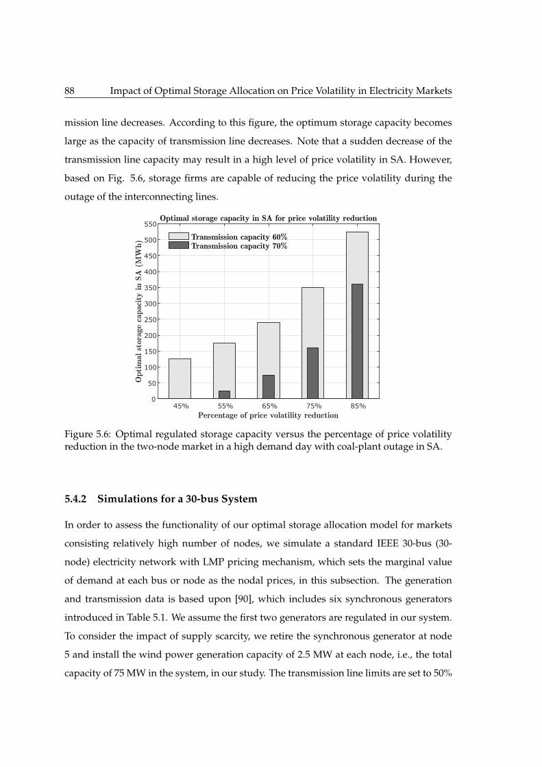
88 Impact of Optimal Storage Allocation on Price Volatility in Electricity Markets
mission line decreases. According to this figure, the optimum storage capacity becomes
large as the capacity of transmission line decreases. Note that a sudden decrease of the
transmission line capacity may result in a high level of price volatility in SA. However,
based on Fig. 5.6, storage firms are capable of reducing the price volatility during the
outage of the interconnecting lines.
Percentage of price volatility reduction45% 55% 65% 75% 85%
Opti
mal
sto
rage
cap
acity
in S
A (
MW
h)
0
50
100
150
200
250
300
350
400
450
500
550Optimal storage capacity in SA for price volatility reduction
Transmission capacity 60%Transmission capacity 70%
Figure 5.6: Optimal regulated storage capacity versus the percentage of price volatilityreduction in the two-node market in a high demand day with coal-plant outage in SA.
5.4.2 Simulations for a 30-bus System
In order to assess the functionality of our optimal storage allocation model for markets
consisting relatively high number of nodes, we simulate a standard IEEE 30-bus (30-
node) electricity network with LMP pricing mechanism, which sets the marginal value
of demand at each bus or node as the nodal prices, in this subsection. The generation
and transmission data is based upon [90], which includes six synchronous generators
introduced in Table 5.1. We assume the first two generators are regulated in our system.
To consider the impact of supply scarcity, we retire the synchronous generator at node
5 and install the wind power generation capacity of 2.5 MW at each node, i.e., the total
capacity of 75 MW in the system, in our study. The transmission line limits are set to 50%

5.5 Conclusion 89
of their values so that some lines would be binding in the solutions.
Table 5.1: Location, capacity and generation cost of synchronous generators in the 30-buselectricity system.
Unit 1 2 3 4 5 6Bus 1 2 5 8 11 13Capacity (MW) 200 80 50 35 30 40Cost ($/MWh) 15 15 35 35 35 35
We divide a day into the off-peak period (10 hours), the peak period (4 hours) and
the shoulder period (10 hours) times. The demand in the off-peak is 10% more than the
demand in the shoulder period whereas the peak demand is 25% more than the shoulder
demand. Given the demand values in [90], we assume the electricity prices are equal to
40, 75 and 50 $/MWh during off-peak, peak, and shoulder periods, respectively.
In the absence of storage, the square root of the price volatility is equal to 250 $/MWh
in the market due to the joint effect of wind power fluctuation and the power-plant retire-
ment. To compute the storage capacity, we use Algorithm 1 with the increment storage
capacity of 15 MWh. According to our numerical results, Algorithm 1 installs the storage
only at node 5, which is the highest price volatile node in the system, in order to meet the
required price volatility level. Fig (5.7) represents the price volatility level after allocating
the storage capacity, calculated by the greedy algorithm 1. The step size of the increment
storage capacity is considered as 15 MWh in each iteration of the algorithm. For instance,
the total storage capacity of 60 MWh at the node 5 is calculated to address the square
root of the price volatility limit of 90 $/MWh. The joint effect of capacity retirement and
high electricity demand at node 5 leads to high level of price volatility after installing
the intermittent wind power capacities in the market and makes the node 5 the likely
candidate for storage allocation to meet the price volatility requirement.
5.5 Conclusion
High penetration of intermittent renewables, such as wind or solar farms, brings high
levels of price volatility in electricity markets. Our study presents an optimization model
which decides on the minimum storage capacity required for achieving a price volatility

90 Impact of Optimal Storage Allocation on Price Volatility in Electricity Markets
Number of iteration0 1 2 3 4 5 6 7 8 9 10
Squ
are
root
of pri
ce v
olat
ility
($/M
Wh)
0
50
100
150
200
250Square root of price volatility in each iteration
Figure 5.7: Square root of price volatility level in the 30-bus system after ten iterations ofAlgorithm 1 with ∆Qst = 15MWh.
target in electricity markets. Based on our numerical results, the impact of storage on the
price volatility in one-node electricity market of SA, two-node market of SA-VIC and the
standard 30-bus IEEE system can be summarized as:
• Storage alleviates price volatility in the market due to the wind intermittency. How-
ever, storage does not remove price volatility completely, i.e. storage stops reducing
the price volatility when it is not profitable.
• The effect of a storage firm on price volatility reduction depends on whether the
firm is regulated or strategic. Both storage types have similar operation behaviour
and price reduction effect when they possess small capacities. For larger capacities,
a strategic firm may under-utilize its available capacity and stop reducing the price
level due to its profit maximization strategy. On the other hand, a regulated storage
firm is more efficient in price volatility reduction because of its social welfare max-
imization strategy. The price level and volatility reduction patterns observed when
storage firms are regulated provide stronger incentives for the market operator to
subsidize the storage technologies.

5.5 Conclusion 91
• Both storage devices and transmission lines are capable of reducing the price volatil-
ity. High levels of price volatility that may happen due to the line maintenance can
be alleviated by storage devices.
• Although many parameters affect the price volatility level of a system, penetration
of intermittent wind power generation in a region makes the region or node highly
price volatile when a synchronous generation capacity outage happens or high load
level is demanded.
Although we showed in this chapter that storage can reduce the average price and
price volatility levels in the market, we study how the mixtures of wind and storage
capacities affect the electricity market prices in Chapter 6.


Chapter 6
Regulated Wind-Storage to Reduce theElectricity Market Price and Volatility
This chapter investigates the impacts of optimal regulated wind and electricity storage allocation
on the average price and the price volatility in electricity markets. A stochastic bi-level optimization
model is proposed for optimal sizing of wind and battery capacities to minimize a wighted sum of the
average market price and price volatility. A fixed budget is allocated on wind and battery capacities
in an upper level problem. The operation of strategic/regulated generation, storage and transmission
players is simulated in a lower level problem using a stochastic (Bayesian) Cournot-based game model.
The Australia’s National Electricity Market (NEM), which is experiencing occasional price peaks
due to closure of a 1600 MW coal power plant and gas price surge, is considered as the case study.
Our simulation results show that investment on regulated wind is more efficient in reducing the
average price, while investment on regulated storage is more effective in price volatility reduction. A
mixture of wind and storage is optimal in minimizing the weighted sum of both average price and
price volatility.
6.1 Introduction
IN THIS chapter, a bi-level stochastic optimization model is proposed for optimal siz-
ing of regulated wind and storage capacities in a single region (node) to minimize
the weighted sum of average price and price volatility taking into account interdepen-
dencies between regions in a wholesale multi-region electricity market. NEM is used as
a case study and a detailed numerical analysis conducted. Our simulation results show
that investment on regulated wind is more efficient in reducing the average price, while
investment on regulated storage is more effective in price volatility reduction.
93

94 Regulated Wind-Storage to Reduce the Electricity Market Price and Volatility
The contributions of this chapter are summarized as follows:
• A bi-level optimization model is proposed to optimally allocate a fixed budget be-
tween regulated wind and storage capacities in a single region to minimize the
weighted sum of average price and price volatility, considering nodal interdepen-
dencies.
• In the upper level problem, the weighted sum of average price and price volatility
in the specified region is minimized by allocating a fixed budget on regulated wind
and storage capacities in that region.
• In the lower level problem, the non-cooperative interaction between strategic and
regulated generation, storage and transmission players in the market is modeled as
a stochastic (Bayesian) Cournot-based game. The equilibrium prices at the lower
level problem, which are calculated based on nonlinear inverse demand functions,
are functions of the regulated wind and storage capacities.
• Considering regulated firms in addition to strategic firms distinguishes our model
in the lower level problem from a standard Cournot game.
• The transmission lines are modeled as profit maximizer market players in our de-
veloped multi-region electricity market model in the lower level problem. Finding
the equilibrium point is computationally far more convenient in electricity market
models with profit maximizer transmission players [91] than in electricity market
models which consider the transmission lines as constraints for their clearing en-
gines [34].
• The existence of Bayesian Nash Equilibrium (Bayes-NE) [81] is established for the
lower level problem, which includes nonlinear inverse demand functions.
The rest of this chapter is organized as follows. Section 6.2 illustrates the system
model and the proposed bi-level optimization problem. The solution approach for find-
ing the market equilibrium is presented in Section 6.3. Section 6.4 provides the simulation
results and Section 6.5 presents the concluding remarks.
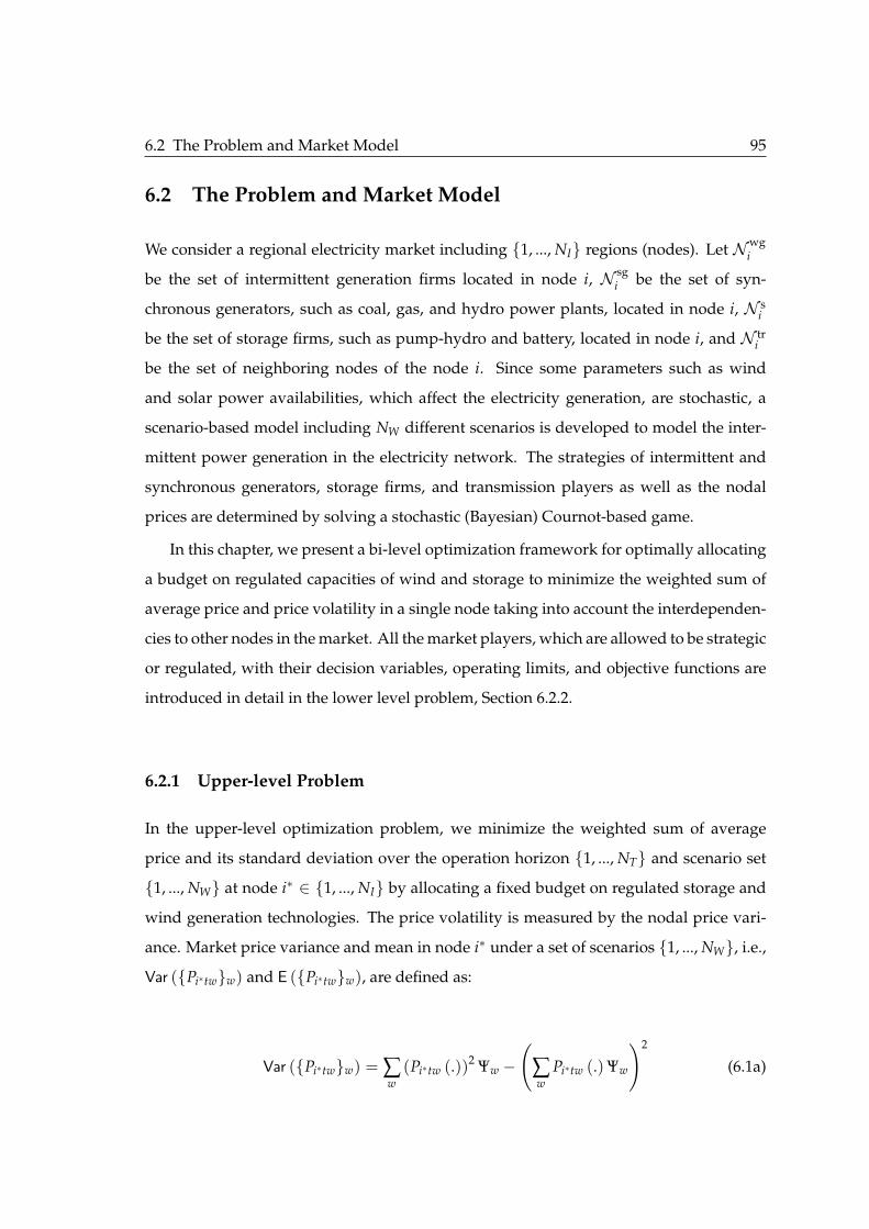
6.2 The Problem and Market Model 95
6.2 The Problem and Market Model
We consider a regional electricity market including 1, ..., NI regions (nodes). Let Nwgi
be the set of intermittent generation firms located in node i, N sgi be the set of syn-
chronous generators, such as coal, gas, and hydro power plants, located in node i, N si
be the set of storage firms, such as pump-hydro and battery, located in node i, and N tri
be the set of neighboring nodes of the node i. Since some parameters such as wind
and solar power availabilities, which affect the electricity generation, are stochastic, a
scenario-based model including NW different scenarios is developed to model the inter-
mittent power generation in the electricity network. The strategies of intermittent and
synchronous generators, storage firms, and transmission players as well as the nodal
prices are determined by solving a stochastic (Bayesian) Cournot-based game.
In this chapter, we present a bi-level optimization framework for optimally allocating
a budget on regulated capacities of wind and storage to minimize the weighted sum of
average price and price volatility in a single node taking into account the interdependen-
cies to other nodes in the market. All the market players, which are allowed to be strategic
or regulated, with their decision variables, operating limits, and objective functions are
introduced in detail in the lower level problem, Section 6.2.2.
6.2.1 Upper-level Problem
In the upper-level optimization problem, we minimize the weighted sum of average
price and its standard deviation over the operation horizon 1, ..., NT and scenario set
1, ..., NW at node i∗ ∈ 1, ..., NI by allocating a fixed budget on regulated storage and
wind generation technologies. The price volatility is measured by the nodal price vari-
ance. Market price variance and mean in node i∗ under a set of scenarios 1, ..., NW, i.e.,
Var (Pi∗tww) and E (Pi∗tww), are defined as:
Var (Pi∗tww) = ∑w(Pi∗tw (.))2 Ψw −
(∑w
Pi∗tw (.)Ψw
)2
(6.1a)

96 Regulated Wind-Storage to Reduce the Electricity Market Price and Volatility
E (Pi∗tww) = ∑w
Pi∗tw (.)Ψw (6.1b)
where Ψw is the probability of scenario w, and Pi∗tw (.) represents the market price in
node i∗ at time t under the scenario w, which is a function of the decision variables, i.e.,
generation, arbitrage and transmission levels, of all players in the lower level problem.
Pi∗tw (.) is a probabilistic function because of the stochastic intermittent generation in our
model.
Given that the wind and storage technologies have unequal lifespans, we compare
their equivalent annual cost and consider the equivalent annual budget in our model.
Considering the relation between the investment cost, I, and its equivalent annual cost,
I, for a technology with lifespan of PL, that is, I = ∑PLy=1
I(1+r)y , the equivalent annual
costs of wind and storage technologies, Iig and Is, become as [92]:
Iig =rIig
1− (1 + r)−PLig (6.2a)
Is =rIs
1− (1 + r)−PLs (6.2b)
where Iig and Is are the total investment costs, and PLig and PLs are the life spans of wind
and storage technologies, respectively. The parameter r represents the discount rate.
Based on the equivalent annual costs of wind and storage technologies, Iig and Is,
IsQs,regi∗ and IigQig,reg
i∗ represent the investment share from the equivalent annual budget,
B, on wind and storage, respectively.
Given the equations for price volatility and average price (6.1a-6.1b), which are func-
tions of the strategy of all firms, and the equations for the equivalent annual cost of wind
and storage technologies (6.2a-6.2b), we define the upper level optimization problem as:
minQig,reg
i∗ ,Qs,regi∗
(1− k)√
Var (Pi∗twtw) + kE (Pi∗twtw) (6.3a)
s.t.
IsQs,regi∗ + IigQig,reg
i∗ = B$ (6.3b)

6.2 The Problem and Market Model 97
where 0 ≤ k ≤ 1 represents the weighting coefficient, Qig,regi∗ is the regulated wind gener-
ation capacity and Qs,regi∗ is the regulated storage capacity in node i∗. Var (Pi∗twtw) is the
normalized level of the average of price volatility levels over the horizon 1, ..., NT, i.e.,
normalized of ∑t Var(Pi∗ tww)NT
, and E (Pi∗twtw) is the normalized level of the average of
mean prices over the horizon 1, ..., NT, i.e., normalized of ∑t E(Pi∗ tww)NT
. The normalized
levels of price volatility and mean price, which are between zero and one, indicate their
ratio with respect to their base values, i.e., with respect to their amounts when there is no
regulated wind and storage firm in the market.
6.2.2 Lower-level Problem
The lower level problem is similar to the one used in Chapter 5, but differs in including
a regulated wind and storage firm in the market.
In the lower level problem, the strategies of all market players and the nodal mar-
ket prices are obtained by solving a stochastic Cournot-based game between intermittent
generators, synchronous generators, storage firms, and transmission firms. Following
the standard Cournot game models [30], any player in our model maximizes its objective
function given the decision variables of other players. Our game model, which considers
different wind and solar power availability scenarios with given probabilities, is consis-
tent with the Bayesian game definition. Players maximize their utility functions over a
set of scenarios with a given probability distribution in a Bayesian game [81]. Note that
the decision variables in the upper level problem, Qig,regi∗ and Qs,reg
i∗ , are the wind and
storage capacity amounts of a regulated wind-storage firm in node i∗.
The market price in node i at time t under scenario w is represented in our model by
an exponential inverse demand function [52]:
Pitw (yitw) = αite−βityitw (6.4)
where αit and βit are positive real values representing in the price function, and yitw is the
net electricity demand in node i at time t under scenario w.
98 Regulated Wind-Storage to Reduce the Electricity Market Price and Volatility
The equality between electricity supply and demand in each node and at any time,
i.e., the the nodal electricity balance, is ensured in our model with the following equa-
tions:
yitw = ∑m∈Nwg
i
qigmitw + ∑
n∈N sgi
qsgnitw + ∑
b∈N si
qsbitw + ∑
j∈N tri
qtrijtw ∀i 6= i∗ (6.5a)
yitw = ∑m∈Nwg
i
qigmitw + ∑
n∈N sgi
qsgnitw + ∑
b∈N si
qsbitw + ∑
j∈N tri
qtrijtw + qig,reg
itw + qs,regitw i = i∗ (6.5b)
where qigmitw is the generation strategy of the mth intermittent generator located in node i,
qsgnitw is the generation strategy of the nth synchronous generator located in node i, qs
bitw
is the charge/discharge strategy of the storage firm b in node i, qtrijtw is the transmission
strategy of line between nodes i and j, and qig,regitw and qs,reg
itw are the wind generation strat-
egy and the storage strategy of the regulated firm in node i∗, respectively, at time t and
under scenario w.
In what follows, we use Pitw (.) to refer to the market price in (6.4).
Intermittent Generators
The mth intermittent generator (wind or solar) in node i determines its best response
strategy by solving the following profit maximization problem:
maxqig
mitw
tw0
NW
∑w=1
Ψw
NT
∑t=1
(Pitw (.)− cig
mi
)qig
mitw (6.6a)
s.t.
qigmitw ≤ ωitwQig
mi ∀t, w (6.6b)
Pitw (.) ≤ Pcap ∀t, w (6.6c)
where qigmitw (decision variable) is the generation level of the intermittent generator m in
node i at time t under scenario w, Qigmi is its maximum generation capacity, and cig
mi is its

6.2 The Problem and Market Model 99
marginal cost of generation. The constraint (6.6b) limits the electricity generation to the
available generation capacity of the firm, considering the energy availability coefficient
ωitw in node i at time t under scenario w. The constraint (6.6c) ensures that the market
price is always less than the cap price Pcap.
Synchronous Generators
The best response strategy of the nth synchronous generator in node i is obtained by
solving the following profit maximization problem:
maxqsg
nitwtw0
NW
∑w=1
Ψw
NT
∑t=1
(Pitw (.)− csg
ni
)qsg
nitw (6.7a)
s.t.
qsgnitw ≤ Qsg
ni ∀t, w (6.7b)
qsgnitw − qsg
ni(t−1)w ≤ Rupni Qsg
ni ∀t, w (6.7c)
qsgni(t−1)w − qsg
nitw ≤ Rdnni Qsg
ni ∀t, w (6.7d)
∑t
qsgnitw ≤ Gni ∀w (6.7e)
Pitw (.) ≤ Pcap ∀t, w (6.7f)
where qsgnitw (decision variable) is the generation level of the synchronous generator n in
node i at time t under scenario w, Qsgni is its generation capacity, and csg
ni is its marginal
cost of generation. The constraint (6.7b) considers the maximum capacity limit and the
constraints (6.7c-6.7d) consider the ramping up and down limits, Rupni and Rdn
ni , respec-
tively. The constraint (6.7e) considers the inter-temporal energy availability Gni, e.g., the
total hydro power generation over a year due to the dam water availability during that
period.
100 Regulated Wind-Storage to Reduce the Electricity Market Price and Volatility
Storage Firms
The best response strategy of the bth storage firm in node i is the solution of the following
profit maximization problem:
maxqdis
bitw,qchbitwtw
0
,qsbitwtw
NW
∑w=1
Ψw
NT
∑t=1
Pitw (.) qsbitw−cs
bi
(qdis
bitw+qchbitw
)(6.8a)
s.t.
qsbitw = ηdis
bi qdisbitw −
qchbitw
ηchbi
∀t, w (6.8b)
qdisbitw ≤ ζdis
bi Qsbi ∀t, w (6.8c)
qchbitw ≤ ζch
bi Qsbi ∀t, w (6.8d)
0 ≤t
∑k=1
(qch
bikw − qdisbikw
)∆ ≤ Qs
bi ∀t, w (6.8e)
Pitw (.) ≤ Pcap ∀t, w (6.8f)
where qchbitw and qdis
bitw (decision variables) are the charge and discharge levels of the stor-
age firm b in node i at time t under scenario w, respectively, qsbitw (intermediate decision
variable) is the net charge/discharge level, csbi is the marginal cost of charge/discharge,
and ηchbi and ηdis
bi are the charging and discharging efficiencies, respectively. The equal-
ity (6.8b) indicates the net outflow or inflow of electricity, the constraints (6.8c) and (6.8d)
limit the output/input energy flow of the firm, with coefficients ζdisbi and ζch
bi , respectively.
The parameters ζchbi and ζdis
bi indicate the percentage of the storage capacity Qsbi that can
be charged or discharged during time period ∆. The constraint (6.8e) limits the total
stored energy to its maximum capacity, assuming that the storage devices are initially
fully discharged.

6.2 The Problem and Market Model 101
Transmission Firms
The best response strategy of the transmission line (interconnector) between nodes i and
j is obtained by solving the following profit maximization problem:
maxqtr
jitw,qtrijtw
tw
NW
∑w=1
Ψw
NT
∑t=1
(Pjtw (.) qtr
jitw + Pitw (.) qtrijtw
) (1− γtr
ij
)+ γtr
ij
(Pjtw (.)−β jt
+Pitw (.)−βit
)(6.9a)
s.t.
qtrijtw = −qtr
jitw ∀t, w (6.9b)
−Qtrij ≤ qtr
ijtw ≤ Qtrij ∀t, w (6.9c)
Pktw (.) ≤ Pcap k ∈ i, j, ∀t, w (6.9d)
where qtrijtw (decision variable) is the electricity transmitted from node j to node i at time
t under scenario w, and Qtrij is the capacity of transmission line between nodes i and j.
The transmission firm between nodes i and j is a strategic player when γtrij is zero and is
a regulated player when γtrij is one. It is discussed in [52] that maximizing Pjt (.) qtr
jitw +
Pitw (.) qtrijtw is equal to maximizing the profit from electricity transmission between nodes
i and j. Besides, it is shown in Appendix B that maximizing Pjtw(.)−β jt
+ Pitw(.)−βit
is equivalent
to maximizing the social welfare when the transmission firm between nodes i and j is
regulated. Note that the electricity markets with regulated transmission firms are called
electricity markets with transmission constraints in the literature, e.g., [20,35]. The constraint
(6.9b) ensures that electricity does not flow simultaneously in both directions of the line,
and the constraint (6.9c) limits the electricity flow between nodes i and j to the capacity
of the line.
102 Regulated Wind-Storage to Reduce the Electricity Market Price and Volatility
Regulated Wind-Storage Firm
The best response strategy of the regulated wind-storage firm in node i∗ is determined
by solving the following optimization problem:
maxqig,reg
i∗ tw
tw0
,
qdis,regi∗ tw ,qch,reg
i∗ tw
tw0
,qs,regi∗ twtw
NW
∑w=1
Ψw
NT
∑t=1
Pi∗tw (.)−βi∗t
− cig,regi∗ qig,reg
i∗tw − cs,regi∗
(qdis,reg
i∗tw + qch,regi∗tw
)(6.10a)
s.t.
qig,regi∗tw ≤ ωi∗twQig,reg
i∗ ∀t, w (6.10b)
qs,regi∗tw = η
dis,regi∗ qdis,reg
i∗tw −qch,reg
i∗tw
ηch,regi∗
∀t, w (6.10c)
qdis,regi∗tw ≤ ζ
dis,regi∗ Qs,reg
i∗ ∀t, w (6.10d)
qch,regi∗tw ≤ ζ
ch,regi∗ Qs,reg
i∗ ∀t, w (6.10e)
0 ≤t
∑k=1
(qch,reg
i∗kw − qdis,regi∗kw
)∆ ≤ Qs,reg
i∗ ∀t, w (6.10f)
Pi∗tw (.) ≤ Pcap ∀t, w (6.10g)
where qig,regi∗tw (decision variable) is the wind (intermittent) generation level of the regu-
lated firm in node i∗ at time t under scenario w, Qig,regi∗ is its maximum wind generation
capacity, and cig,regi∗ is its marginal cost of wind generation. Moreover, qch,reg
i∗tw ,qdis,regi∗tw (deci-
sion variables), and qs,regi∗tw (intermediate decision variable) are the charge, discharge and
net charge/discharge levels of the regulated firm in node i∗ at time t under scenario w, re-
spectively. The constraint (6.10b) is similar to the constraint in the wind generation prob-
lem (6.6b), and the constraints (6.10c)-(6.10f) are similar to the constraints in the storage
arbitrage problem (6.8b)-(6.8e). The reason why maximizing the Pi∗ tw(.)−βi∗ t
− cig,regi∗ qig,reg
i∗tw −
cs,regi∗
(qdis,reg
i∗tw + qch,regi∗tw
)is equivalent to maximizing the social welfare for the regulated
wind-storage firm in our problem is based on the discussion in Appendix B on regulated
firms.

6.3 Solution Approach 103
6.3 Solution Approach
Here, the bi-level storage and wind allocation problem reducing the average price and
price volatility is transformed into a single-level Mathematical Problem with Equilibrium
Constraints (MPEC). The equivalent single-level (MPEC) problem is solved by a uniform
line search algorithm, which is different from our methodology for solving the single-
level problem in Chapter 5.
6.3.1 Solution Method for the lower level problem
The regulated wind and storage capacities are the only variables that couple the scenar-
ios in the lower level problem. Therefore, for any regulated wind and storage capacity
amounts, each scenario of the lower level problem can be solved autonomously and the
market equilibrium can be obtained by solving the KKT conditions of all firms. The exis-
tence of the Bayes-NE solution at the lower level problem is stated in Proposition 6.1.
Proposition 6.1. For any vector of regulated wind and storage capacity amounts, [Qig,regi∗ , Qs,reg
i∗ ],
the lower level game admits a Bayes-NE.
Proof: The objective function of any firm in the game is continuous and quasi-
concave in its strategy, and their strategy space is non-empty, compact and convex. There-
fore, according to Theorem 1.2 in [79], the lower level game admits a Bayes-NE.
In the lower level problem, the nodal market prices depend on the regulated wind
and storage capacities through the constraints (6.10b) and (6.10d-6.10f). This dependency
allows us to minimize the objective function on the upper level problem using the optimal
values of regulated wind and storage capacities.
6.3.2 Solution Method for the equivalent single level problem
Imposing the KKT conditions of all firms as constraints in the optimization problem (6.3),
we can transform our bi-level problem into the following single-level optimization prob-
lem:

104 Regulated Wind-Storage to Reduce the Electricity Market Price and Volatility
min (1− k)√
Var (Pi∗twtw) + kE (Pi∗twtw) (6.11a)
s.t.
(6.3b) (6.11b)
KKT (6.6a− 6.6c) (6.11c)
KKT (6.8a− 6.8 f ) (6.11d)
KKT (6.7a− 6.7 f ) (6.11e)
KKT (6.9a− 6.9d) (6.11f)
KKT (6.10a− 6.10g) (6.11g)
where the optimization variables are the regulated wind and storage capacities, the bid-
ding strategies of all firms, and the set of all Lagrangian multipliers. Note that the feasible
region is not necessarily convex or even connected because of the nonlinear complemen-
tary constraints. It is possible to write the equivalent single level problem (6.11) as a
Mixed-Integer Non-Linear Problem (MINLP), but the large number of integer variables
makes the problem computationally infeasible.
Considering the equality constraint (6.3b), there is just one decision variable on the
upper level problem. We perform a uniform line search on the variable Qig,regi∗ , i.e., the sin-
gle decision variable of the upper level problem, with N iterations. We increase the reg-
ulated wind capacity by ∆Qig,reg and decrease the regulated storage capacity by ∆Qs,reg,
which is a function of ∆Qig,reg, and find the Bayes-NE solution of the lower level game
at each iteration. Comparing the average price and price volatility calculated at differ-
ent iterations, we find the optimal regulated wind and storage allocation, as described in
Algorithm 2.
6.4 Case Study and Simulation Results
In this section, we apply our bi-level price management framework to Australia’s Na-
tional Electricity Market (NEM). The inverse demand functions in our model are cal-

6.4 Case Study and Simulation Results 105
Algorithm 2 The line search (N-step) algorithm for finding the wind-storage allocation.
∆Qig,reg = BNIig
initial point← Qig,reg = 0, Qs,reg = BIs
for iteration = 0 : N doiteration=iteration+1Qig,reg
i∗ (iteration)←Qig,regi∗ (iteration− 1)+∆Qig,reg
Qs,regi∗ ← B−IigQig,reg
i∗Is
q?(iteration)← Lower level problem Bayes−NEE(iteration),Var(iteration)← (6.1b, 6.1a) at Bayes−NE
end for
Qig,regi∗
∗← find
Qig,regi∗
(min((1− k)√
Var(
Qig,regi∗
)+ kE
(Qig,reg
i∗
)))
Qs,regi∗
∗ ← B−IigQig,regi∗
∗
Is
ibrated with historical demand and price data from the year 2016. Different types of
electricity generation firms, such as coal, gas, hydro, biomass, and wind, with total gen-
eration capacity of 46 GW were active in NEM in 2016 [12]. In our numerical study, we
consider 365 scenarios each representing a 24-hour wind power availability and electric-
ity demand profiles. The realistic data in different regions of NEM from the year 2016 is
used to generate the scenario set (Source of data: AEMO). Note that all the prices are in
Australian dollar.
6.4.1 Impact of Generation Capacity, Gas Price and Transmission Line on Av-erage Price and Price Volatility in NEM
In this subsection, we first study the average price and price volatility in the NEM by
considering two cases. In our primary case, the NEM market is simulated based on the
available data in 2016. In our secondary case, the Hazelwood coal power plant in VIC is
closed down, the gas price in total NEM is increased, and the Basslink transmission line,
between VIC and TAS, which was under maintenance in 2016, is restarted in compari-
son to the primary case. Table 6.1 compares the simulated wholesale electricity prices in
five regions of NEM in the primary and secondary cases. Our simulation results show
that the average price of electricity increases in all regions, about 14.27% in NEM, due to
Hazelwood power plant closure and gas price surge. The highest rate of price increment

106 Regulated Wind-Storage to Reduce the Electricity Market Price and Volatility
belongs to VIC, about 40.33%, where the coal plant was located, following by its neigh-
boring region SA with 19.80%. According to our numerical results, restarting the Basslink
interconnector between VIC and TAS reduces the impacts of coal plant closure and gas
price surge on the electricity price in TAS, which increases just by 3.58% in average.
Table 6.1: Wholesale electricity prices ($/MWh) in five-node NEM market in primaryand secondary cases.
SA QLD TAS VIC NSW NEMPrimary Case 108.97 72.32 99.64 57.48 58.81 67.27Secondary Case 130.55 78.94 103.20 80.66 61.65 76.87Change% 19.80 9.16 3.58 40.33 4.83% 14.27
Our calculation also shows that price volatility increases in NEM after the coal plant
closure and gas price surge. The square root of price volatility increases by 17.7% in NEM,
where VIC experiences the highest increase rate of 41.5%. The Basslink transmission line
also suppresses the price volatility in TAS due to the Hazelwood closure and gas price
surge.
6.4.2 Managing the Average Price and Price Volatility by Only Regulated Windor Only Regulated Storage
In this subsection, we study the impact of installing only regulated wind or only regu-
lated storage on the average price and price volatility in VIC, where the coal power plant
is closed down. We start our simulations with the equivalent annual budget of 300 m$,
and perform the sensitivity analysis with other amounts of the equivalent annual bud-
get, between zero and 300 m$, later. Considering the investment cost of 2400 $/kW and
lifespan of 25 years, the equivalent annual cost is 96 $/(kW.yr) for wind generation. Also,
with the investment cost of 600 $/kWh and lifespan of 10 years, the equivalent annual
cost is 60 $/(kWh.yr) for battery storage. Therefore, the equivalent annual budget of 300
m$ is almost equivalent to 5000 MWh battery capacity or 3125 MW wind capacity.
Fig. 6.1 shows the impact of installing only 5000 MWh regulated battery on the
wholesale electricity prices in VIC. According to this figure, the regulated battery in VIC
charges at off-peak times and discharges at peak hours, i.e., makes profit from electric-

6.4 Case Study and Simulation Results 107
ity arbitrage. The charge/discharge of the installed battery approximately results in the
average peak price reduction of 47 $/MWh and the average off-peak price increment of
16 $/MWh in VIC. The average wholesale electricity price in VIC decreases from 80.6
$/MWh to 72.9 $/MWh due to the addition of 5000 MWh regulated battery.
hr2 4 6 8 10 12 14 16 18 20 22 24
Whol
esal
e P
rice
($/
MW
h)
20
40
60
80
100
120
140
Bat
tery
Char
ge/D
isch
arge
(M
W)
-1500
-1000
-500
0
500
1000
1500
Price before Battery AdditionPrice after Battery Addition Battery Charge/Discharge
Figure 6.1: Mean (over 365 scenarios) wholesale electricity prices in VIC before and afteraddition of only 5000 MWh regulated battery storage capacity.
Fig. 6.2 shows the impact of installing only 3125 MW regulated wind on the wholesale
electricity prices in VIC. The regulated wind in our model with capacity of 3125 MW
generates electricity with average level of 975 MW, i.e., with capacity factor of 31%, in
VIC. The generation of the regulated wind firm results in the average peak and off-peak
wholesale price reductions of 28 $/MWh and 5 $/MWh, respectively, in VIC. The average
wholesale electricity price in VIC decreases from 80.6 $/MWh to 62 $/MWh due to the
3125 MW wind capacity addition. This observation confirms that wind power generators
are more efficient in average price reduction than storage firms.
Fig. 6.3a and 6.3b compare the impact of a regulated wind with that of a regulated
storage on the average price and the price volatility, respectively, in VIC when the equiv-
alent annual budget increases from zero to 300 m$. It can be seen that for different levels
of budget, i.e., different levels of capacity, the regulated storage is more efficient in re-
ducing the price volatility whereas the regulated wind is more efficient in reducing the

108 Regulated Wind-Storage to Reduce the Electricity Market Price and Volatility
hr2 4 6 8 10 12 14 16 18 20 22 24
Mea
n W
hol
esal
e P
rice
($/
MW
h)
20
40
60
80
100
120
140
Win
d G
ener
atio
n (
MW
)
0
200
400
600
800
1000
1200Price before Wind AdditionPrice after Wind Addition Wind Generation
Figure 6.2: Mean (over 365 scenarios) wholesale electricity prices in VIC before and afteraddition of only 3125 MW regulated wind generation capacity.
average price. Given the equivalent annual budget of 300 m$, the regulated storage and
the regulated wind reduce the square root of price volatility in VIC by 71.14 % and 53.55
%, respectively. However, with the same equivalent annual budget, regularized storage
and wind firms reduce the average price in VIC by 10.04 % and 29.08 %, respectively. This
observation shows the effectiveness of storage in price volatility reduction and wind in
average price reduction.
Moreover, in addition to mean price and price volatility reduction impacts, the cost
analysis of the regulated wind and regulated storage can affect the investment decisions.
Fig. 6.3c indicates the cost analysis of the regulated wind and regulated storage in VIC
when the equivalent annual budget varies from zero to 300 m$. The life time rate of re-
turn less than 100 % shows a financially unprofitable investment. Based on this figure,
the regulated wind is financially profitable in VIC when the equivalent annual invest-
ment cost is less than 300 m$, but the regulated storage makes profit in VIC when the
equivalent annual investment cost is less than 100 m$. Note that future reduction in
battery cost makes the large investments on batteries profitable.

6.4 Case Study and Simulation Results 109
(a)30 120 210 300
Mea
n W
hol
esal
e P
rice
($/
MW
h)
50
55
60
65
70
75
(b)Equivalent Annual Budget on Wind or Storage (m$)
30 120 210 300
Squ
are
Roo
t of
Pri
ceV
olat
ility
($/M
Wh)
40
60
80
100
120
140
160
(c)30 120 210 300
Life
Tim
e R
ate
of R
eturn
(%
)
20
40
60
80
100
120
140
160
180WindStorage
Figure 6.3: The mean price, the square root of price volatility, and the life time rate of re-turn for only regulated wind and only regulated battery allocation versus the equivalentannual budget in VIC.
6.4.3 Managing the Average Price and Price Volatility by Mixture of Regu-lated Wind and Storage in VIC
In this subsection, we study the impact of jointly optimal regulated wind and storage
allocation on the mean price and price volatility. Fig. 6.4 illustrates the normalized mean
wholesale price as well as the normalized square roof of price volatility for different mix-
tures of wind and battery allocation with the equivalent annual budget of 300 m$ in VIC.
The mean wholesale prices are normalized with base value of 73 $/MWh, which is the
average price in the market before adding regulated wind-storage capacities, and the
square root of price volatilities are normalized with the base value of 143 $/MWh, which
is the square root of price volatility in the market before adding regulated wind-storage
capacities. According to Fig. 6.4, the increase of the regulated wind share, ξ, (or equiv-
alently, the decrease of regulated storage share, 1-ξ) results in lower average prices but
higher price volatility levels in the market, and vice versa. Therefore, depending on the
importance of average price or price volatility, i.e., the coefficient k, the total budget can
be allocated on a mixture of regulated wind and battery capacities.
Fig. 6.5 shows the budget allocation share between regulated wind (ξ) and regulated

110 Regulated Wind-Storage to Reduce the Electricity Market Price and Volatility
Figure 6.4: Normalized mean wholesale price and square root of price volatility for differ-ent mixtures of regulated wind and regulated battery with the equivalent annual budgetof 300 m$ in VIC.
battery (1− ξ) when the weighting coefficient of price volatility and average price in the
upper level problem (6.3), k, varies from zero to one. The logistic shape of the optimal
budget share function with respect to the weighting coefficient k verifies our observa-
tions regarding the impacts of wind and storage firms on the price. The optimal share of
regulated wind is more than that of the regulated storage when average price reduction
is prioritized, i.e., when 0.5 ≤ k ≤ 1. Similarly, when price volatility reduction is more
important, i.e., when 0 ≤ k ≤ 0.5, the optimal share of regulated battery is more than that
of the regulated wind. The decision making on the budget share is highly sensitive with
respect to parameter k when the average price and the price volatility are almost equally
important, i.e., 0.4 ≤ k ≤ 0.6.
6.5 Conclusion
Closure of base-load coal power plants, and gas price surge may increase the average
price and price volatility in electricity markets. Our study presents an optimization
framework which allocates a budget on regulated wind and storage capacities in order

6.5 Conclusion 111
Figure 6.5: The budget allocation share between the regulated wind and the regulatedbattery as a function of the weighting factor k with the equivalent annual budget of 300m$ in VIC.
to minimize the weighted sum of the average price and the price volatility. Based on our
numerical results in NEM, the impacts of regulated wind and storage on average price
and price volatility can be summarized as:
• In a multi-region electricity market, closure of a coal power plant in one region may
affect the electricity prices in other regions. After the closure of Hazelwood power
plant in VIC, the average price and volatility increased in VIC and its neighbor-
ing regions, but not in TAS. Reopening the Basslink interconnector between VIC
and TAS in 2017 prevented to observe significant price increase in TAS despite the
Hazelwood closure and gas price surge.
• Both storage and wind affect the average price and price volatility in electricity mar-
kets. Storage technologies can reduce the price and the price volatility by electricity
price arbitrage. Being spread across the network, wind turbines can also decrease
the price and volatility in electricity markets. However, storage is more efficient in
price volatility reduction than wind whereas wind is more efficient in average price
reduction.

112 Regulated Wind-Storage to Reduce the Electricity Market Price and Volatility
• Although disptchable generators are more efficient in reducing the price volatility,
wind turbines, if being spread across the network, can also reduce the price volatil-
ity level in the market. In our model, a single node represents an entire state, and
hence, incorporates diversity of wind generation across a large geographic region
that counteracts natural intermittency of wind generation.
• Based on the importance of average price and price volatility, a mix capacity of
regulated wind and storage can be allocated in a region to reach the desired level
of price and volatility in the market.
• Wind turbine, with small or large capacity, is already a competent technology which
is able to recover its life time cost in the market, but storage technology is econom-
ical just in small to medium size, e.g., battery capacity larger than 1300 MWh in
VIC is not economically profitable. Future reduction of technology costs can make
it economical to install larger batteries in the market.
• Our developed model is generalized to consider any type of storage technology.
However, in our case study, we studied the battery storage, which is likely to pen-
etrate in large scale in Australia’s electricity market in future.
The operation of generators, storage utilities and the transmission lines are the de-
cision variables in our developed operational wholesale electricity market models. In
Chapters 7 and 8, we develop long term electricity market models, which include op-
eration and investment decision variables, and use them to design long-term emission
abatement and fast response capacity support policies in the market.

Part III
Designing Incentive Policies inElectricity Markets
113


Introduction to Part III 115
Introduction to Part III
IN THIS Part, we develop long-term planning Cournot-based electricity market mod-
els, which are used to design incentive policies on reducing the emission and main-
taining the system reliability in the network. The designed policies are in forms of tax
and subsidy.
In Chapter 7, a generation expansion electricity market model, including strategic
and regulated generation firms, is developed. All players in the game maximize their
utilities subject to a emission cap constraint, the dual variable of which is used to design
the emission tax required to achieve the emission reduction target in the market.
In Chapter 8, an electricity market evolution model, including strategic and regulated
generation, storage and transmission firms, is developed. Any player in the game maxi-
mizes its utility subject to an emission intensity reduction constraint and a fast response
dispatchable generation constraint. The dual variable of the emission constraint is used
to design the tax/subsidy incentives required to achieve the emission intensity target and
the dual variable of the fast response constraint is used to design the tax/subsidy incen-
tives required to achieve the reliability (balance between demand and supply) target in
the market.


Chapter 7
Long-Term Stochastic Planning inElectricity Markets with a Carbon Cap
Constraint
Carbon price in an electricity market provides incentives for carbon emission abatement and renew-
able generation technologies. Policies constraining or penalizing carbon emission can significantly
impact the capacity planning decisions of both fossil-fueled and renewable generators. Uncertainties
due to intermittency of various renewable generators can also affect the carbon emission policies. This
chapter proposes a Cournot-based long-term capacity expansion model taking into account a carbon
cap constraint for a partly concentrated electricity market dealing with stochastic renewables using
a Bayesian game. The stochastic game is formulated as a centralized convex optimization problem
and solved to obtain a Bayes-Nash Equilibrium (Bayes-NE) point. The stochastic nature of a generic
electricity market is illustrated with a set of scenarios for wind availability, in which three generation
firms (coal, gas, and wind) decide on their generation and long-term capacity investment strategies.
Carbon price is derived as the dual variable of the carbon cap constraint. Embedding the carbon cap
constraint in the game leads to more investment on renewable generators and less on fossil-fueled
power plants. However, higher levels of intermittency from renewable generation leads to higher car-
bon prices required to meet the carbon cap constraint in the market. This paves the way towards
storage technologies and diversification of distributed generation as means to encounter intermittency
in renewable generation.
7.1 Introduction
IN THIS chapter, we theoretically develop a stochastic game-theoretic Cournot-based
model which calculates a Bayes-NE point in partly concentrated electricity markets,
having both strategic and perfectly competitive (fringe) generation players. In addition
117

118 Long-Term Stochastic Planning in Electricity Markets with a Carbon Cap Constraint
to generation portfolio, the firms decide on expanding their capacities during the study
period dealing with the uncertainties due to intermittency of certain renewables, e.g.,
stochasticity of wind and solar. Players decide on new capacity investment and their
generation by considering a set of scenarios for wind and solar availability and a carbon
cap constraint during the study period. The dual variable of the carbon cap constraint
is used to calculate the the carbon price required to meet the targeted carbon emission
cap in the market. The stochastic nature of our model enables us to find the effect of
intermittent renewables on the carbon price.
Moreover, capacity retirement and remaining value of new generation capacities are
considered in our model. It means that power plants become retired once time passes
their plant life and the remaining value of each new invested technology at the end of the
study period is subtracted from its investment cost. For instance, a generator having T′
years plant life pays just 1T′ of the investment cost in our model if it decides to install a
new capacity exactly at the last year in our model. However, the annualized investment
cost ($/MW/yr) is an alternative way instead of considering the remaining values of
new invested technologies, e.g. in [32]; although it is not hard to construct an unusual
example where this is not true.
The contributions of this chapter include the following:
• A long-term stochastic generation capacity expansion model with an emission cap
constraint is developed which captures the strategic behavior of generation firms.
A set of scenarios is included in the model due to the intermittency of wind and
solar energies.
• The carbon price required to restrict the emission in the market, which is due to the
greenhouse gas control or green network policies, is calculated based on the dual
variable of the emission cap constraint at the Bayes-NE point of the game.
• The structure of our long-term model enables us to find the intertemporal expan-
sion and retirement of the generation capacities and the remaining value of new
generation capacities in the market.
The rest of this chapter presents the wholesale electricity market model with strategic

7.2 Game-Theoretic Formulation of Long-term Wholesale Electricity Market 119
and perfectly competitive generation players in Section 7.2, illustrative results in Section
7.3, and ends with a discussion and conclusion in Section 7.4.
7.2 Game-Theoretic Formulation of Long-term Wholesale Elec-tricity Market
In a Cournot-Nash wholesale electricity market model, the generation players (firms)
make their decisions strategically in order to maximize their utility functions, and the
equilibrium price is equal to the inverse demand function. However, participants in a
partly concentrated liberalized electricity market are either strategic or perfectly compet-
itive. The strategic players decide on their generation to set the price in the market as
price maker players, i.e., they hold market power, while the perfectly competitive play-
ers either are not large enough to affect the price (fringe participants) or are regulated to
not benefit from their market power.
At the same time, the intermittent wind and solar powers are stochastic, which brings
a great deal of uncertainty to the market. Decisions on new capacities have to be made
considering a set of scenarios for wind and solar availabilities during the study period
taking also into account a carbon emission cap constraint. Accordingly, we define the fol-
lowing extended Cournot-based Bayesian game model to find the long-term equilibrium
point of the market.
7.2.1 Game Definition and Bayes-Nash Equilibrium
In the well-known Cournot electricity market model, several strategic generation com-
panies make their generation decisions non-cooperatively given that the price follows
the inverse demand function. However, we study a partly concentrated market in which
there is perfectly competitive generation companies besides the oligopoly generators.
In a Bayesian game, players maximize their expected utility over alternative possibil-
ities with a known probability distribution [81]. Availability of the stochastic renewables
is captured in our model in a set of scenarios with given probabilities, consistent with the
Bayesian game definition.

120 Long-Term Stochastic Planning in Electricity Markets with a Carbon Cap Constraint
Definition 2. A perfectly competitive (PC) player does not have the market power to raise the
wholesale price, where a strategic player may deliberately withholds its available capacity to in-
crease the price.
Let k ∈ K = 1, ..., K be in the set of generation firms (generators) participating in
the electricity market, y ∈ Y = 1, ..., Y be in the set of times with length of ∆Yy (yr),
s ∈ S = 1, ..., S be in the set of load zones (like seasons in a year) with length of ∆Ss
(dayyr ), t ∈ T = 1, ..., T be in the set of sub-load zones (like off-peak, shoulder and peak
times in a day) with length of ∆Tt (hr
day ), and w ∈ W be in the set of scenarios on wind
availability in our Bayesian game. Total duration of sub-load zone t that repeats on load
zone s from period y is ∆lyst = ∆Yy∆Ss∆Tt hours.
In our game G, firm k decides on its generation qkystw (∀y, s, t, w) and new capacities
Qnewky (∀y) in order to maximize its utility Uk. We assume that the generator k has con-
stant marginal cost of production ($/MWh), ck ≥ 0, constant capacity maintenance cost
($/MW/yr), mk ≥ 0, and constant investment cost ($/MW), Invk ≥ 0.
Definition 3. A non-cooperative Bayesian game among K = 1, ..., K players having the deci-
sion variables q = [q1, ..., qK] and Qnew = [Qnew1 , ..., Qnew
K ] that aim to maximize their expected
profit U over scenarios w ∈ W with probabilities Ψw is defined as G = K, (q, Qnew) 0, U .
In a Cournot-based electricity market model, such as [7], the commonly-used linear
price P follows the inverse demand function with intercept of α and slope of β:
Pystw = αyst − βystDystw ∀y, s, t, w (7.1)
where Dystw is the total electricity demand at time (y, s, t) and under scenario w.
Players in the market are categorized into two groups:
• perfectly competitive (γk = 1): which could be a set of fringe participants or a
regulated competitive firm.
• strategic (γk = 0) or Cournot players.

7.2 Game-Theoretic Formulation of Long-term Wholesale Electricity Market 121
Player k calculates its best responses, i.e., q∗k = q∗kystwy,s,t,w, Qnewk∗ = Qnew
ky∗y, by
solving the following utility maximization problem:
maxqk ,Qnew
kQtotal
k ,D0
Uk : ∑y
1(1 + r)y
(∑
w,s,tΨw∆lyst
((αyst−βystDystw)qkystw + γk
βyst
2q2
kystw−ckqkystw
)
−mk∆YyQtotalky − InvkQnew
ky
)+
1(1 + r)Y max(0,
PLk + y−Y− 1PLk
)InvkQnewky (7.2)
s.t.
Dystw = ∑k
qkystw ∀y, s, t, w (7.3)
qkystw ≤ Qtotalky ∀y, s, t, w (7.4)
Qtotalky =
y
∑y′=max(1,y−PLk+1)
Qnewky′ +
Y0
∑y”=Y0−PLk+y+1
Qoldk,y” ∀y (7.5)
qkystw − qkys(t−1)w ≤ Rupk Qtotal
ky ∀y, s, t, w (7.6)
qkys(t−1)w − qkystw ≤ Rdnk Qtotal
ky ∀y, s, t, w (7.7)
qkystw ≤ ωkystwQtotalky ∀y, s, t, w (7.8)
∑s,t
qkystw ≤ RAky ∀y, w (7.9)
where qk, Qnewk are independent variables and Qtotal
k , D are intermediate variables.
For strategic player k, the objective function (7.2) sums the expectation of revenue,
qkystw(αyst − βystDystw), minus the operation cost, ckqkystw, with probabilities of Ψw over
scenarios w ∈ W , the maintenance cost, mkQtotalky , and the investment cost on the new ca-
pacity, InvkQnewky , excluding its remaining value at the end time, max(0, PLk+y−Y−1
PLk)InvkQnew
ky .
The revenues and costs over periods Y are discounted with respect to a specific base year
Y0 assuming discount rate r(%/∆Yy). However, for a perfectly competitive player, the
objective function has additional term βyst2 q2
kystw, which is equivalent to the market sur-
plus loss when the player k is not perfectly competitive.
The supply/demand balance equation (7.3) equalizes the net consumption with the
total generation. Capacity constraint (7.4) binds generation to its total capacity. Equality

122 Long-Term Stochastic Planning in Electricity Markets with a Carbon Cap Constraint
(7.5) (This is the modified version of capacity constraint in [93]) sums the new capacities
Qnewky′ and historical ones Qold
k,y” which are not retired at time y as the total capacity Qtotalky .
Constraints (7.6) and (7.7) consider the ramping up and down limits of the generator. The
period-by-period power availability limit, applicable to all generators especially intermit-
tent wind turbines, is shown in (7.8). Lastly, constraint (7.9) considers the inter-temporal
generation limits due to planned/forced outages or fuel scarcity.
7.2.2 Carbon Price Calculation as a Dual Variable
Due to local and global concerns on greenhouse gases, there are upper bound restrictions
on carbon emission in electricity generation. When fossil-fueled generators burn coal,
natural gas or petroleum to produce electricity, they emit CO2 gas as a side product.
Considering the policy of pollution generation control in the market, we can calculate the
desired carbon price required to achieve the upper bound on carbon emission constraint:
∑k,s,t,w
Ψw∆lystEFkqkystw ≤ ECO2y (1− φ) : µy ∀y (7.10)
where ECO2y is the upper limit of CO2 (tonne) emission in electricity industry during time
y, and EFk is the CO2 emission coefficient of generator k (tonneCO2/MWh). The dual
variable of constraint (7.10), µy, is proportional to the target carbon price ($/tonneCO2)
at time y that policy makers must announce to control the carbon pollution in the mar-
ket. Note that the dual variable of the carbon cap constraint must be consistent in all
individual profit maximization problems of all players in the NE point. Considering the
first order optimality conditions of all individual problems (Karush-Kuhn-Tucker condi-
tions), it can be shown that the variable (1 + r)yEFkµy is the pollution tax that generator
k pays during time y per each unit of electricity generation qkystw.
7.2.3 Solving the Game as a Centralized Optimization Problem
The Bayes-NE point of the game including both strategic and perfectly competitive play-
ers at generation level, with the objective functions and constraints explained in Section

7.3 Numerical Analysis 123
(7.2.1), can be computed by solving the following centralized optimization problem:
maxq,Qnew
Qtotal,D≥0
∑y
1(1+r)y
(∑
s,t,wΨw∆lyst
((αyst−
βyst
2Dystw)Dystw−∑
k
βyst
2(1−γk)qkystw
2+ckqkystw
)
−∑k
mk∆YyQtotalky + InvkQnew
ky
)+
1(1 + r)Y ∑
kmax(0,
PLk + y−Y− 1PLk
)InvkQnewky (7.11)
s.t.
(7.3)− (7.10) ∀k
where q, Qnew are independent variables and Qtotal, D are intermediate variables.
The objective function (7.11) sums the total surpluses of demand and supply in the
market minus the market surplus loss regarding the suppliers’ strategic behaviors. The
centralized optimization problem is subjected to the constraints of all individual players’
profit maximization problems.
In this chapter, the centralized quadratic optimization problem is solved to find the
Bayes-NE point of the game. However, it is possible to write the KKT conditions of indi-
vidual profit maximization problems and solve it as a Linear Complementarity Problem
in distributed fashion.
7.3 Numerical Analysis
For illustrative purposes, we numerically investigate a generic single-node system com-
prising three generation firms- coal, gas, and wind- planning for capacity installation
during next 25 years, including 5 time steps (∆Yy=5 years), consisting of peak (∆Tpeak=4
hours a day), shoulder (∆Tshoulder=10 hours a day) and off-peak (∆Toff-peak=10 hours a
day) load zones for a whole year (∆S=365 days in a year). The parameters for the inverse
demand function (7.1) are listed in Table 7.1, which indicate the highest values for α and
the lowest values for β at peak load zones. Assuming electricity demand increases over
years, the parameter α is raised with rate of 5% every 5 years.
Considering investment, maintenance, operation and fuel costs in addition to life time
of technologies and their ramping up and down specifications, which are listed in Table

124 Long-Term Stochastic Planning in Electricity Markets with a Carbon Cap Constraint
Table 7.1: The parameters for the inverse demand function.
y,∆y = 5 years
1 2 3 4 5
αy,t
peak 240 252 264 277 291shoulder 200 210 220 231 243off-peak 160 168 176 185 194
βy,t
peak .08 .08 .08 .08 .08shoulder .1 .1 .1 .1 .1off-peak .12 .12 .12 .12 .12
7.2 [94], the generation firms decide on participating in the market. The parameter γ is
zero for coal and gas-fueled generators, which shows they play strategically, and is one
for the wind firm, which means that it plays perfectly competitively.
Table 7.2: Costs and technology specifications of generation firms.
firms Investment($/kW)
Maintenance($/kW/yr)
Operation& Fuel($/kWh)
Plant Life(5years)
RampUp &Dn
coal 2500 25 0.015 8 0gas 1000 10 0.055 6 0.9wind 3000 30 0 4 1
The base values for wind power availability is assumed 40% at off-peak times, 30%
at shoulder times, and 10% at peak times. In wind availability scenarios, wind power
availability is assumed to vary σ% above and under its base values as shown in Figure
7.1.
Employing the commercial solver CONOPT in GAMS software [95], the centralized
quadratic optimization problem is solved with the mentioned input data to calculate the
Bayes-NE point of the game.
7.3.1 Impact of Carbon Cap on Capacity Planning
Total carbon production of the system without any pollution control policy is calcu-
lated in our model based on the emission factors of 0.93 tonneCO2 /MWh for coal and
.55 tonneCO2 /MWh for gas as listed in Table 7.3.
The simulation is repeated for two different values of carbon reduction percentage
φ ∈ 20, 40% and is compared with no carbon cap scenario in Figure 7.2. Total car-

7.3 Numerical Analysis 125
Off-peak Peak Shoulder
Avail (%)
10
30
40
100
2σ %
2σ %
2σ %
Figure 7.1: Normalized wind capacity availability (ωt) during off-peak, shoulder, andpeak load zones, distributed on [(1-σ)E(ω), (1+σ)E(ω)] with the given expected valueE(ω) .
Table 7.3: Total CO2 emission every five years in the system with no carbon cap con-straint.
y (5-years) 1 2 3 4 5ECO2
y(million tonne)
31.8 33.0 34.3 35.6 37.0
bon emission in the system becomes restricted, using the constraint (7.10) in the game
model. Restricting the total carbon emission in the system leads to more investment on
renewables and less on fossil-fueled power plants, especially coal-fueled generators. The
price increase motivates renewables to invest more in our game model with carbon cap
constraint.
7.3.2 Impact of Wind Stochasticity on Carbon Price
The dual variable of the carbon cap constraint at the Bayes-NE point is used to calcu-
late the carbon price. Policy makers can announce the carbon price as a tax to make
the power plants comply with the pollution policies in the market. Stochasticity arising
from intermittent generators impacts the values of carbon price. Figure 7.3 represents the
calculated carbon price at every five-year period respectively for φ ∈ 20%, 60% car-
bon emission reduction policies in two scenarios of deterministic (σ = 0) and stochastic

126 Long-Term Stochastic Planning in Electricity Markets with a Carbon Cap Constraint
Figure 7.2: Capacity investment Qtotal and its change ∆Qtotal due to carbon cap constraintwith coefficient φ ∈ 20, 40%.
(σ = 60%) wind power availability. Simulation results show that higher carbon prices are
calculated when stricter emission reduction is targeted in the market, and also higher car-
bon prices are required to meet the carbon cap constraint when the intermittentcy from
renewable generators is higher in the market.
7.3.3 Impact of Wind Player’s Strategic Behavior on Capacity Planning
We compare the capacity planning of all generators when wind firm participating in the
market is strategic or perfectly competitive. The wind player representing all wind tur-
bines in our model is a profit maximizer player in the strategic wind case and a fringe
player in the perfectly competitive wind case. It is observed that proportionally the coal
firm installs more generation capacity, the gas firm slightly lowers its capacity expansion
rate, and the wind player installs much less new generation capacity in the strategic wind
case compared to the perfectly competitive wind case, as is shown in Figure 7.4.

7.3 Numerical Analysis 127
Figure 7.3: Carbon pricing for different CO2 emission reduction scenarios (φ ∈ 20 %, 60%).
years5 10 15 20 25
MW
0
200
400
600
800
1000
1200
1400
1600
(PC Wind)
years5 10 15 20 25
MW
0
200
400
600
800
1000
1200
1400
1600
(Strategic Wind)
coalgaswind
Figure 7.4: New capacity installation Qnew considering wind strategy (perfectly compet-itive and strategic).
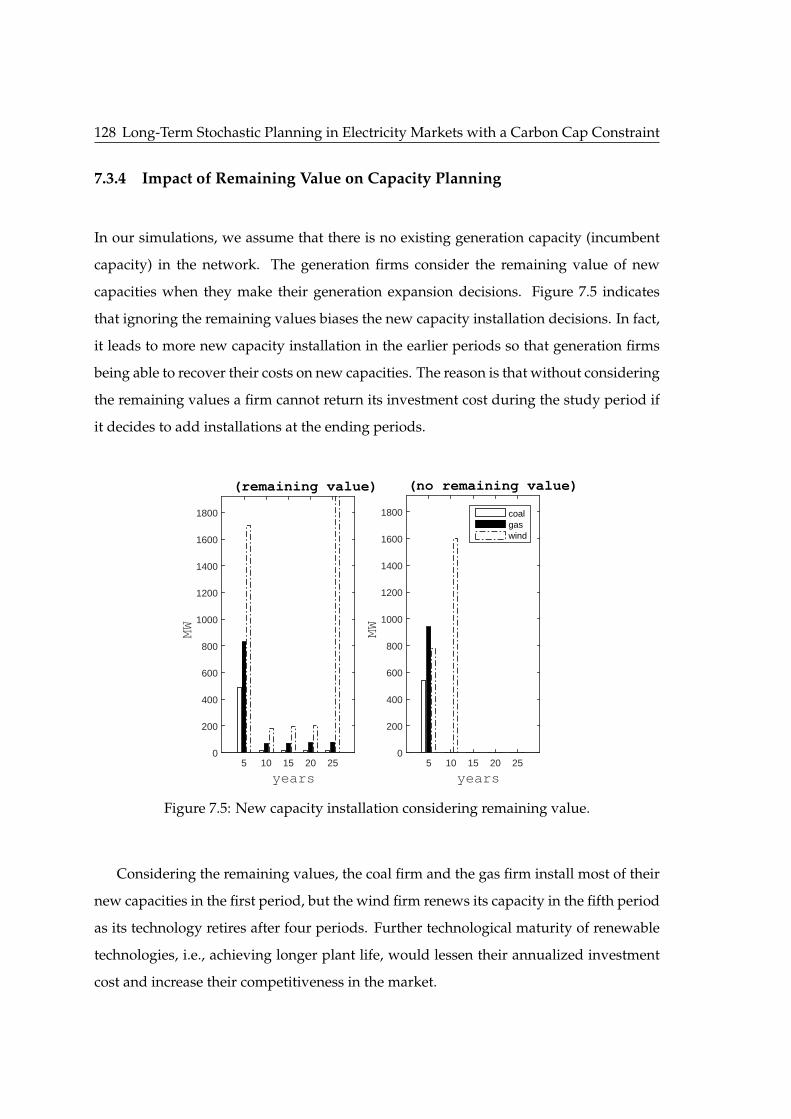
128 Long-Term Stochastic Planning in Electricity Markets with a Carbon Cap Constraint
7.3.4 Impact of Remaining Value on Capacity Planning
In our simulations, we assume that there is no existing generation capacity (incumbent
capacity) in the network. The generation firms consider the remaining value of new
capacities when they make their generation expansion decisions. Figure 7.5 indicates
that ignoring the remaining values biases the new capacity installation decisions. In fact,
it leads to more new capacity installation in the earlier periods so that generation firms
being able to recover their costs on new capacities. The reason is that without considering
the remaining values a firm cannot return its investment cost during the study period if
it decides to add installations at the ending periods.
years5 10 15 20 25
MW
0
200
400
600
800
1000
1200
1400
1600
1800
(remaining value)
years5 10 15 20 25
MW
0
200
400
600
800
1000
1200
1400
1600
1800
(no remaining value)
coalgaswind
Figure 7.5: New capacity installation considering remaining value.
Considering the remaining values, the coal firm and the gas firm install most of their
new capacities in the first period, but the wind firm renews its capacity in the fifth period
as its technology retires after four periods. Further technological maturity of renewable
technologies, i.e., achieving longer plant life, would lessen their annualized investment
cost and increase their competitiveness in the market.

7.4 Conclusion 129
7.4 Conclusion
New capacity expansion is dependent on the market price expectation, which is highly
affected by renewable energies availability. Moreover, policy makers can intervene in the
market via setting tax on carbon emission to meet their goals. The modeling analysis pre-
sented in this chapter studies the impacts of carbon cap constraint on long-term capacity
investment decisions of generation firms facing stochastic renewable power availability.
Based on our model and the simulation results, the impacts of carbon cap on capacity
expansion of three coal, gas and wind generation firms are as following:
• Carbon cap constraint in the game model results in proportionally more new re-
newable and less fossil-fueled generation capacity, especially less coal-fueled ca-
pacity.
• Dual variable of the carbon cap constraint at the Bayes-NE point is used to calculate
the carbon price in our model. Policy makers can announce it in the market as
carbon emission tax, which leads to invest more on renewable capacities.
• Higher levels of intermittency from renewables makes them financially less attrac-
tive. Higher tax on carbon emission can make renewables able to compete with
fossil-fueled generators even if renewables are highly intermittent. The difference
in the carbon price can be used towards storage technologies and diversification of
distributed generation as means to encounter intermittency in renewable genera-
tion.
• We intend to extend our stochastic game model to study the long term investment
on storage technologies and transmission lines in addition to generation technolo-
gies. In the future, storage technologies, similar to renewables, are expected to
achieve longer plant life and experience high capacity expansion due to reduction
in their annualized investment costs.
• The input data in our model and simulations is consistent with the real data in
Australias electricity market, and we can accept the conclusions in this chapter for
the electricity markets which are similar to NEM.

130 Long-Term Stochastic Planning in Electricity Markets with a Carbon Cap Constraint
By considering a carbon cap constraint in our developed long-term electricity market
model, we designed the carbon tax amounts required to achieve the carbon abatement
policies in the market. In Chapter 8, we design tax/subsidy policies required to achieve
emission intensity reduction and fast response capacity support policies in the market by
extending our long-term electricity market model.

Chapter 8
Designing Tax&Subsidy IncentivesTowards a Green and Reliable
Electricity Market
Incentive schemes and policies play an important role in reducing carbon emissions from electricity
generation. This chapter investigates tax and subsidy incentives towards a reliable and low emis-
sion electricity market, using Australia’s National Electricity Market (NEM) as a case study. A
game-theoretical Cournot-based electricity market expansion model is developed, which calculates the
capacity investment and retirement of any strategic/regulated generation, storage, and transmission
player for multi investment periods, taking into account Emission Intensity Reduction and Fast Re-
sponse Dispatchable Capacity constraints. Based on the dual variables of the emission reduction and
the fast response generation constraints at the Nash Equilibrium solution of the game, the incentive
policies (tax/subsidy) on emission and fast response capacity are designed, respectively. The simula-
tion results for Australia’s NEM during 2017-2052, indicates how large investment on thermal solar
technology, battery storage and transmission lines supports high level of Variable Renewable Energy,
wind and solar, penetration in a green and reliable electricity market. Improvement of new technolo-
gies and their cost reduction trajectory show that NEM does not need any emission incentive policy
for up to 45% emission intensity reduction by 2052. However, higher emission reduction targets
require imposing taxes on pollutant generators and subsidizing clean generators.
8.1 Introduction
IN THIS chapter, a strategically competitive electricity market expansion model, which
includes the emission intensity reduction and fast response dispatchable capacity
constraints, is proposed. The Nash Equilibrium (NE) solution of our model is used to
131

132 Designing Tax&Subsidy Incentives Towards a Green and Reliable Electricity Market
design the incentive policies on emission reduction and fast response dispatchable ca-
pacity support. The dual variable of the emission constraint at the Nash Equilibrium
solution of the game is used to design the emission incentive policies and the dual vari-
able of the fast response dispatchable capacity constraint at the NE point is used to design
the capacity incentive policies. In other words, the model is developed to illustrate the
pathway towards a reliable and low emission future.
The contributions of this chapter are summarized as follows:
• A game-theoretical Cournot-based electricity market expansion model is proposed,
which solves an unified operation and installation problem, to find the future ca-
pacity mix of generation, storage and transmission players in the market. All play-
ers in our model can be either strategic or perfectly competitive.
• Using the dual variable of the emission intensity reduction constraint at the NE
point of our model, we calculate the emission tax and subsidy that generators are
required to pay and receive for a targeted low emission market.
• Using the dual variable of the fast response generation constraint at the NE point
of our model, we calculate the capacity tax and subsidy that generators and storage
firms are required to pay and receive in order to maintain the system reliable.
Under the proposed framework, an electricity generation mix for Australia’s NEM is
designed such that the emission intensity target is achieved and the reliability is main-
tained. The incentive policies on emission and fast response capacity are also calculated
using the NE solution of the game.
The rest of this chapter is organized as follows. The strategically competitive electric-
ity market expansion model is formulated in Section 8.2. The equilibrium analysis of the
problem and the solution method are presented in Section 8.3. The simulation results are
presented in Section 8.4. The conclusion remarks are discussed in Section 8.5.

8.2 Strategically Competitive Electricity Market Expansion Model 133
8.2 Strategically Competitive Electricity Market Expansion Model
In this section, we develop an electricity market expansion model which consists of
generation, storage and transmission firms trading electricity in a multi-node energy-
only wholesale electricity market. Let N igi be the set of intermittent generators, such as
wind/PV farms and roof-top PVs, located in node i, N sgi be the set of synchronous gen-
erators, such as coal, gas, hydro and thermal solar power plants, located in node i, N sti
be the set of storage firms, such as pump-hydros and batteries (cooperatively controlled
or non-cooperative), located in node i, andN tri be the set of transmission lines connected
to node i.
The market expansion problem is formulated as a Cournot-based game among the
generation, storage and transmission players, which are introduced in detail in Section
8.2.4. At the NE solution of the game, the capacity investment strategies of the firms,
their biding strategies as well as the equilibrium nodal prices are calculated. The market
expansion game is solved under the emission intensity and fast response generation con-
straints, which their dual variables are used to calculate the tax and subsidy incentives.
8.2.1 Inverse Demand Functions
In our model, the electricity price in node i at investment period y, with duration of five
years, and load time t, with duration of one hour, is given by the following, commonly-
used linear inverse demand function:
Piyt(
Diyt)= αiyt − βiytDiyt, (8.1)
Diyt = ∑m∈N ig
i
qigmiyt + ∑
n∈N sgi
qsgniyt + ∑
b∈N sti
qstbiyt + ∑
j∈N tri
(ηtr
ij qtrijyt − qtr
jiyt
)∀i, y, t (8.2)
where αiyt and βiyt are positive real values for the inverse demand function in node i
at period y, and load time t. Besides, qigmiyt is the electricity generation of intermittent

134 Designing Tax&Subsidy Incentives Towards a Green and Reliable Electricity Market
generator m in region i , qsgniyt is the electricity generation of synchronous generator n in
region i, qstbiyt is the electricity flow from storage firm b in node i, and qtr
ijyt is the electricity
flow from node j to node i at period y, and load time t. Note that the total amount of
power supply from the generation, storage and transmission firms in node i is equal to
the nodal net electricity demand, which represents the nodal electricity balance in our
work.
Although roof-top PVs and residential batteries do not participate in the wholesale
market, their operation affects the market price, i.e., shifts the inverse demand function
up or down. Thus, instead of modeling the roof-top PVs and residential batteries on the
demand side, we equivalently model them on the supply side as perfectly competitive
players.
8.2.2 Total Capacity and Investment Functions
In our model, any player can retrofit its capacity at any investment period y. The total
capacity of each firm at period y, Qy, is the sum of incumbent (old) capacities, Qoldy , which
are given as exogenous input to the model, and new capacities, Qnewy , which are decision
variables of players, as:
Qy(Qnewy′≤y) =
y
∑y′=max(1,y−PL+1)
Qnewy′ +
Y0
∑y′′=Y0−PL+y+1
Qoldy′′ (8.3)
where PL denotes the plant life of the corresponding technology of the firm, and Y0 is the
base year in our study. Note that firms in our model are able to decommission their ca-
pacities at any period before they reach their plant life and each technology must become
retired in our model when it reaches its plant life.
Market expansion models which assume annualized investment cost for technolo-
gies do not take capacity retirement into account [32]. Instead of using the annualized
investment cost, we consider the whole technology costs and deduct the end of period
remaining value of new capacities [33] from their investment costs in our model as:

8.2 Strategically Competitive Electricity Market Expansion Model 135
Invy =
(1− max(0, PL + y− NY − 1)
PL
)˜Inv (8.4)
where ˜Inv is the actual investment cost of a unit and Invy is the modified value of invest-
ment cost at period y in our model. For instance, in a 25-year period simulation study,
NY = 25, if a firm with the technology plant life of 20 years decides to install a new unit
at year 21, it just pays 14 of the actual investment cost in our model. Note that we include
the yearly maintenance costs of technologies as part of their investment costs and do not
consider them separately.
8.2.3 The Emission and Capacity Incentive Policies
An upper bound on the emission intensity is considered in our model to ensure the emis-
sion intensity reduction in the market as:
∑i,t
∑n∈N sg
i
qsgniytEFni
∑i,t
∑n∈N sg
i
qsgniyt + ∑
m∈N igi
qigmiyt
≤(
1− αERy
)EICO2
Y0: µER
y ∀y (8.5)
where EICO2Y0
is the CO2 emission intensity of the whole electricity sector at base (refer-
ence) year Y0, αERy is the desired percentage of emission intensity reduction at period y
relative to the base period Y0, EFni is the emission factor of fossil-fueled synchronous gen-
erator n in node i. The dual variable associated with this constraint, i.e., µERy , corresponds
to the required emission tax/subsidy (first incentive policy) to achieve a level of emission
intensity, as shown in Section 8.3.3.
The second incentive policy is calculated based on the fast response dispatchable ca-
pacity constraint. The constraint limits the total VRE generation to a proportion of fast
response generation during each investment period to ensure adequacy of fast response
capacity in the network as:

136 Designing Tax&Subsidy Incentives Towards a Green and Reliable Electricity Market
∑t
∑n∈N sg
i
αsg,FRni qsg
niyt + ∑b∈N st
i
αst,FRbi qdis
biyt
≥ αFR ∑t
∑m∈N ig
i
qigmiyt : µFR
iy ∀i, y (8.6)
where αFR is the fast response proportion coefficient, αsg,FRni is a binary coefficient which
is one if firm n in region i is a fast response synchronous generator, such as gas-fired or
hydro, αst,FRbi is a binary coefficient which is one if firm b in region i is a pump-hydro or a
cooperatively controlled battery, and qdisbiyt is the electricity discharge level of the storage
firm b in node i. It is also shown in Section 8.3.3 that the required annual capacity sub-
sidy/tax to ensure that there is enough fast response capacity in the network is calculated
based on the dual variable of the fast response constraint, µFRiy :
Note that we can reduce the coefficient αFR, i.e., the need for fast response capacity
to achieve diversity dividends, by spreading the wind and solar generation across the
network, which smooths the generation and ramping up and down of the total regional
intermittent electricity generation [96].
8.2.4 The Market Expansion Game
In this subsection, we introduce the market expansion game, the utility function of play-
ers and their decision variables. In our model, each firm decides on its expansion capacity
and bidding strategies over the planning horizon, being either strategic or regulated.
Definition 8.1. A strategic (price maker) firm sets its strategies over the time horizon maximizing
its aggregate expected profit, but a regulated (price taker) firm aims to maximize the social welfare
[77].
In what follows, the variable µ indicates the associated Lagrange or dual variable of
its corresponding constraint, the price function Piyt (.) refers to (8.1) and the total capacity
function Q(.) refers to (8.3).

8.2 Strategically Competitive Electricity Market Expansion Model 137
Intermittent Generation Firms
The mth intermittent generator, i.e., wind or solar farm or roof-top PVs, in node i maxi-
mizes its profit by solving the following optimization problem:
maxqig
miyt
yt
Qig,newmiy
y
0
∆l ∑y,t
Piyt (.) qigmiyt −
(cig
miqigmiyt +
digmi2 qig
miyt2)+ γ
igmi
βiytqigmiyt
2
2
(1 + r)y −∑y
InvigmiyQig,new
miy
(1 + r)y
(8.7a)
s.t.
qigmiyt ≤ Aig
mitQigmiy(.) : µ
igmiyt ∀y, t (8.7b)
Qigmiy(.) ≤ Cig
mi : µig,Cmiy ∀y, t (8.7c)
(8.5), (8.6) (8.7d)
where Qig,newmiy and Qig
miy(.) are the new capacity (variable) and the total generation capac-
ity (function) of the intermittent (VRE) firm m in node i at period y, respectively. The first
term in the summation in (8.7a) is the net present value of electricity generation revenue,
the second term represents the generation cost, which is quadratic (with coefficients cigmi
and digmi) and reflects that cheaper renewable energy sites are deployed first, the third
term denotes the regulation surplus when γigmi is one, given the discount rate r over the
periods y ∈ 1, ..., NY. The last term in (8.7a) is the total investment cost of new capac-
ities, with unitary investment cost of Invigmiy, over the periods. Depending on the binary
parameter γigmi, the mth intermittent generation firm in node i behaves strategically or in a
regulated manner. The firm acts strategically when γigmi is zero or acts as a regulated firm
when γigmi is one. Considering the
βiytqigmiyt
2
2 in the objective function, the firm becomes reg-
ulated (price taker), which helps to increase the competition and consequently the social
welfare in the market. The constraint (8.7b) considers the regional intermittent energy
availability coefficient in load time t, Aigmit, and the constraint (8.7c) limits the electricity
generation to the maximum potential capacity, Cigmi, e.g., the roof-top PV installation area

138 Designing Tax&Subsidy Incentives Towards a Green and Reliable Electricity Market
limit.
Synchronous Generation Firms
The strategy of the nth synchronous generator, i.e., coal, gas, biomass, hydro or thermal
solar firms, in node i is obtained by solving the following optimization problem:
maxqsg
niyt
yt
Qsg,newniy
y
0
∆l ∑y,t
Piyt (.) qsgniyt − csg
ni qsgniyt + γ
sgni
βiytqsgniyt
2
2
(1 + r)y −∑y
InvsgniyQsg,new
niy
(1 + r)y (8.8a)
s.t.
qsgniyt ≤ Asg
ni Qsgniy(.) : µ
sgniyt ∀y, t (8.8b)
qsgniyt − qsg
niy(t−1) ≤ Rupni Asg
ni Qsgniy(.) : µ
sg,upniyt ∀y, t (8.8c)
qsgniy(t−1) − qsg
niyt ≤ Rdnni Asg
ni Qsgniy(.) : µ
sg,dnniyt ∀y, t (8.8d)
∑t
qsgniyt ≤ RAsg
niy : µsg,RAniy ∀n, i, y (8.8e)
(8.5), (8.6) (8.8f)
where Qsg,newniy and Qsg
niy(.) are the new capacity (variable) and total generation capacity
(function) of the synchronous firm n in node i at period y. The parameter csgni represents
the firm’s marginal operation and fuel cost of electricity generation and the parameter
Invsgniy is its unitary investment cost. Depending on the binary parameter γ
sgni , the nth
synchronous generator in node i acts strategically when γsgni is zero or acts as a regulated
firm when γsgni is one. The constraint (8.8b) limits the electricity generation to its energy
flow capacity with availability coefficient Asgni . Constraints (8.8c) and (8.8d) ensure that
the nth synchronous generator meets its ramping limits, with ramping up and down co-
efficients Rupni and Rdn
ni , and constraint (8.8e) limits the electricity generation during period
y to energy availability limit RAsgniy, e.g. the dam water availability limit for hydros.

8.2 Strategically Competitive Electricity Market Expansion Model 139
Storage Firms
The strategy of the bth storage firm, i.e., pump-hydro, or cooperatively controlled or
non-cooperative batteries, in node i is obtained by solving the following optimization
problem:
maxqdis
biyt,qchbiyt
yt0
Qstf,newbiy ,Qstv,new
biy
y0
qstbiyt
yt
∆l ∑y,t
Piyt (.) qstbiyt + γst
biβiytqst
biyt2
2
(1 + r)y −∑y
Invstv
biyQstv,newbiy + Invstf
biyQstf,newbiy
(1 + r)y
(8.9a)
s.t.
qstbiyt = ηdis
bi qdisbiyt −
qchbiyt
ηchbi
: µstbiyt ∀y, t (8.9b)
qdisbiyt ≤ Ast
biQstf
biy(.) : µdisbiyt ∀y, t (8.9c)
qchbiyt ≤ Ast
biQstf
biy(.) : µchbiyt ∀y, t (8.9d)
0 ≤t
∑t′=1
(qch
biyt′ − qdisbiyt′
)∆ ≤ Ast
biQstv
biy(.) : µst,minbiyt , µst,max
biyt ∀y, t (8.9e)
qdisbiytq
chbiyt = 0 : µdis/ch
biyt ∀y, t (8.9f)
(8.6) (8.9g)
where Qstv,newbiy and Qstf,new
biy are the new volume and flow capacity (variable), and Qstv
biy(.)
and Qstf
biy(.) are the total volume and flow capacity (function) of the storage firm b in node
i at period y, respectively. Note that the unit for volume capacity is MWh (energy) and
for flow capacity is MW (power). The parameters Invstv
biy and Invstf
biy are the firm’s unitary
volume and flow investment costs, respectively. Depending on the binary parameter γstbi,
the bth storage firm in node i acts strategically when γstbi is zero and acts as a regulated
firm when γstbi is one. The equality (8.9b) defines the net output/input flow of electricity,
qstbiyt, from/to storage firm b in node i. The constraints (8.9c) and (8.9d) limit the energy
flow (discharge qdisbiyt and charge qch
biyt) of the firm to its flow (discharge/charge) capacity

140 Designing Tax&Subsidy Incentives Towards a Green and Reliable Electricity Market
with availability factor Astbi. Constraint (8.9e) ensures the volume capacity limit of the
storage firm is always met. Finally, constraint (8.9f) prevents the storage firm charge and
discharge simultaneously, which is the only non-linear constraint in our model.
Transmission Firms
The strategy of the transmission line between nodes i and j, which buys and sells elec-
tricity in regions it connects, is obtained by solving the following optimization problem:
maxqtr
jiyt,qtrijyt
yt
Qtr,newijy ,Qtr,new
jiy
y
0
∑y,t
∆l
((ηtr
ij Pjyt (.)− Piyt (.))
qtrjiyt
(1 + r)y +
(ηtr
ij Piyt (.)− Pjyt (.))
qtrijyt
(1 + r)y +
γtrij
(ηtr
ij2βiyt + β jyt
) qtrijyt
2
2 +(
ηtrij
2β jyt + βiyt
) qtrjiyt
2
2 − ηtrij
(β jyt + βiyt
)qtr
ijytqtrjiyt
)(1 + r)y −
∑y
Invtrijy
2
(Qtr,new
ijy + Qtr,newjiy
)(1 + r)y (8.10a)
s.t.
qtrijyt ≤ Atr
ij Qtrijy(.) : µtr
ijyt ∀y, t (8.10b)
Qtr,newijy = Qtr,new
jiy : µtr,Qijy ∀y (8.10c)
where Qtr,newijy and Qtr
ijy(.) are the new capacity (variable) and the total transmission ca-
pacity (function) of the transmission firm between nodes i and j at period y. The first
term in summation in (8.10a) is the electricity profit of transmitting electricity from node
i to node j, the second term is the backward profit, the third term denotes the regula-
tion surplus and the last term is the total investment cost of new capacities, with uni-
tary investment cost of Invtrijy. Depending on the binary parameter γtr
ij , the transmission
line between nodes i and j acts strategically when γtrij is zero or acts as a regulated firm
when γtrij is one. Note that the electricity markets with regulated transmission lines are
discussed as electricity markets with transmission constraints in the literature, e.g., [20, 35].

8.3 Solution Methodology 141
The constraint (8.10b) limits the electricity flow to the capacity of transmission lines with
availability coefficient Atrij , and the constraint (8.10b) ensures that transmission capacity
on both directions of the line is equal in our model.
Note that the profit maximization problem (8.10a) looks more complex than our pre-
vious formulation in [52] because of considering the transmission efficiency, ηtrij , which
was missing before.
8.3 Solution Methodology
In this section, we first provide a game-theoretic analysis of the market expansion game
between generation, storage and transmission players. Next, we explain a method for
solving the game based on a Mixed Complementarity Problem (MCP).
8.3.1 Game-theoretic Analysis of the Market Expansion Model
To solve the market expansion game, we need to study the best response functions of
all firms participating in the market. Then, any intersection of all firms’ best response
functions will be a NE. At the NE strategy of the game, no player has any incentive to
unilaterally deviate its strategy from the NE point.
Note that (8.9f), which is nonlinear, is the only constraint in our model that violates
the sufficient conditions of Theorem 4.4 in [71] for existence of NE point. However, in
our numerical results, we find the NE point of the game by varying the initial point of
the optimization algorithm.
The orthogonal constraints corresponding to emission and fast response capacity with
dual variables of µERy and µFR
iy , respectively, which exist in best response equation sets of
all players, are given by:
∑i,t
∑n∈N sg
i
qsgniytEFni
∑i,t
∑n∈N sg
i
qsgniyt + ∑
m∈N igi
qigmiyt
≤(
1− αERy
)EICO2
Y0⊥ µER
y ≥ 0 (8.11a)
142 Designing Tax&Subsidy Incentives Towards a Green and Reliable Electricity Market
∑t
∑n∈N sg
i
αsg,FRni qsg
niyt + ∑b∈N st
i
αst,FRbi qdis
biyt
≥ αFR ∑t
∑m∈N ig
i
qigmiyt ⊥ µFR
iy ≥ 0 (8.11b)
Best Responses of Intermittent Generation Firms
The best response of the intermittent generator m in node i, given the strategies of other
firms in the market, satisfies the necessary and sufficient Karush-Kuhn-Tucker (KKT)
conditions (t ∈ 1, ..., NT; y ∈ 1, ..., NY):
∆lPiyt (.)−
(cig
mi + digmiq
igmiyt
)− βiytq
igmiyt
(1− γ
igmi
)(1 + r)y − µ
igmiyt +
(1− αER
y
)EICO2
Y0µER
y − αFRµFRiy
≤ 0 ⊥ qigmiyt ≥ 0 (8.12a)
−Invigmiy
(1 + r)y −min(NY ,y+PLig
mi−1)
∑y′=y
(µ
ig,Cmiy′ −∑
tAig
mitµigmiy′t
)≤ 0 ⊥ Qig,new
miy ≥ 0 (8.12b)
qigmiyt ≤ Aig
mitQigmiy(.) ⊥ µ
igmiyt ≥ 0 (8.12c)
qigmiyt ≤ Cig
mi ⊥ µig,Cmiyt (8.12d)
where the perpendicularity sign, ⊥, indicates that one of the adjacent inequalities must
at least be satisfied as an equality [73].
Best Responses of Synchronous Generation Firms
The best response of the synchronous generator n in node i, given the collection of strate-
gies of other firms in the market, is obtained by solving the following KKT conditions
(t ∈ 1, ..., NT; y ∈ 1, ..., NY):
∆lPiyt (.)− csg
ni − βiytqsgniyt
(1− γ
sgni
)(1 + r)y − µ
sgniyt + µ
upniy(t+1) − µ
upniyt − µdn
niy(t+1) + µdnniyt − µ
sg,RAniy
−(
EFni −(
1− αERy
)EICO2
Y0
)µER
y + αsg,FRni µFR
iy ≤ 0 ⊥ qsgniyt ≥ 0 (8.13a)

8.3 Solution Methodology 143
−Invsgniy
(1 + r)y + ∑t
Asgni
min(NY ,y+PLsgni−1)
∑y′=y
(µsgniy′t + Rup
ni µupniy′t + Rdn
ni µdnniy′t) ≤ 0 ⊥ Qsg,new
niy ≥ 0
(8.13b)
qsgniyt ≤ Asg
ni Qsgniy(.) ⊥ µ
sgniyt ≥ 0 (8.13c)
qsgniyt − qsg
niy(t−1) ≤ Rupni Asg
ni Qsgniy(.) ⊥ µ
upniyt ≥ 0 (8.13d)
qsgniy(t−1) − qsg
niyt ≤ Rdnni Asg
ni Qsgniy(.) ⊥ µdn
niyt ≥ 0 (8.13e)
∑t
qsgniyt ≤ RAsg
niy ⊥ µsg,RAniy ≥ 0 (8.13f)
Best Responses of Storage Firms
The best response of the storage firm b in node i, given the collection of strategies of other
firms in the market, is obtained by solving the following KKT conditions (t ∈ 1, ..., NT;
y ∈ 1, ..., NY):
∆lPiyt (.)− βiytqst
biyt
(1− γst
bi
)(1 + r)y + µst
biyt = 0 (8.14a)
− ηdisbi µst
biyt − µdisbiyt − ∆
NT
∑t′=t
µst,minbiyt′ − µst,max
biyt′ + αst,FRbi µFR
iy + µdis/chbiyt qch
biyt ≤ 0 ⊥ qdisbiyt ≥ 0
(8.14b)
µstbiyt
ηchbi− µch
biyt + ∆NT
∑t′=t
µst,minbiyt′ − µst,max
biyt′ + µdis/chbiyt qdis
biyt ≤ 0 ⊥ qchbiyt ≥ 0 (8.14c)
−Invstv
biy
(1 + r)y + ∑t
Astbi
min(NY ,y+PLstvbi −1)
∑y′=y
µst,maxbiy′t ≤ 0 ⊥ Qstv,new
biy ≥ 0 (8.14d)
−Invstf
biy
(1 + r)y + ∑t
Astbi
min(NY ,y+PLstfbi −1)
∑y′=y
µdisbiy′t + µch
biy′t ≤ 0 ⊥ Qstf,newbiy ≥ 0 (8.14e)
qstbiyt = ηdis
bi qdisbiyt −
qchbiyt
ηchbi
(8.14f)
qdisbiyt ≤ Ast
biQstf
biy(.) ⊥ µdisbiyt ≥ 0 (8.14g)
qchbiyt ≤ Ast
biQstf
biy(.) ⊥ µchbiyt ≥ 0 (8.14h)

144 Designing Tax&Subsidy Incentives Towards a Green and Reliable Electricity Market
0 ≤t
∑t′=1
(qch
biyt′ − qdisbiyt′
)∆ ⊥ µst,min
biyt ≥ 0 (8.14i)
t
∑t′=1
(qch
biyt′ − qdisbiyt′
)∆ ≤ Ast
biQstv
biy(.) ⊥ µst,maxbiyt ≥ 0 (8.14j)
qdisbiytq
chbiyt = 0 (8.14k)
Best Responses of Transmission Firms
Finally, the best response of the transmission firm between nodes i and j, given the collec-
tion of strategies of other firms in the market, can be obtained using the KKT conditions
(t ∈ 1, ..., NT; y ∈ 1, ..., NY):
∆lηtr
ij Piyt (.)− Pjyt (.) +(
1− γtrij
) ((−βiytη
trij
2 − β jyt
)qtr
ijyt + ηtrij
(βiyt + β jyt
)qtr
jiyt
)(1 + r)y − µtr
ijyt
≤ 0 ⊥ qtrijyt ≥ 0 (8.15a)
−Invtrijy
2(1 + r)y + µtr,Q
ijy − µtr,Qjiy + ∑
tAtr
ij
min(NY ,y+PLtrij−1)
∑y′=y
µtrijy′t ≤ 0 ⊥ Qtr,new
ijy ≥ 0 (8.15b)
qtrijyt ≤ Atr
ij Qtrijy(.) ⊥ µtr
ijyt ≥ 0 (8.15c)
Qtr,newijy = Qtr,new
jiy (8.15d)
8.3.2 The Mixed Complementarity Problem
The NE solution is by definition the intersection of best responses of all players. There-
fore, it satisfies the KKT conditions of all market players, that is, (8.11a-8.11b), (8.12a-
8.12d), (8.13a-8.13f), (8.14a-8.14k), and (8.15a-8.15d). Consequently, the NE solution is
the result of the following Mixed Complementarity Problem (MCP):
(8.11a− 8.11b), (8.12a− 8.12d), (8.13a− 8.13 f ), (8.14a− 8.14k), (8.15a− 8.15d)
m ∈ 1, ..., Nigi , n ∈ 1, ..., Nsg
i , b ∈ 1, ..., Nsti , i, j ∈ 1, ..., I, t ∈ 1, ..., NT, y ∈ 1, ..., NY

8.3 Solution Methodology 145
where the decision variables are the bidding strategies of all players, and set of Lagrange
multipliers or dual variables in KKT conditions. We used the PATH solver in GAMS
software to solve the MCP problem.
8.3.3 Interpreting the Dual Variables as Tax and Subsidy
In this subsection, based on dual variable of the emission constraint (8.5), µERy , and dual
variable of the fast response constraint (8.6), µFRiy , at the NE point of the game, we cal-
culate the CO2 emission tax/subsidy and the economic value of fast response capacity,
respectively, in our model.
Firstly, we explain the carbon taxing/subsidizing mechanism in our model. From
equation (8.13a), it is observed that the term (1+r)y
∆l
(EFni −
(1− αER
y
)EICO2
Y0
)µER
y consti-
tutes a portion of the price function, Piyt (.), when qsgniyt is positive, which can be inter-
preted as the tax/subsidy the synchronous generator n in node i must pay/receive per
each MWh electricity generation at period y. Similarly, it can be seen in equation (8.12a)
that the term (1+r)y
∆l
(1− αER
y
)EICO2
Y0µER
y is equal to the subsidy the intermittent renew-
able generator m in node i, which is wind or solar, receives per each MWh electricity
generation at period y.
Secondly, we explain the fast response capacity mechanism in our mode. The term
αFRµFRiy in equation (8.12a), the term α
sg,FRni µFR
iy in equation (8.13a), and the term αst,FRbi µFR
iy
in equation (8.14b) constitute a portion of the price function, Piyt (.), when qigmiyt, qsg
niyt and
qdisbiyt are positive, respectively. Therefore, at the NE solution the term
∆l ∑t
αFRµFRiy qig
miyt
Qigmiy(.)
is equal
to the fast response capacity tax that in average one MW intermittent generator pays
per each period y, and∆l ∑
tα
sg,FRni µFR
iy qsgniyt
Qsgniy(.)
, and∆l ∑
tαst,FR
bi µFRiy qdis
biyt
Qst,fbiy(.)
are equal to the fast response
capacity subsidy that in average one MW synchronous generator and one MW storage
firm receives per each period y, respectively.
8.3.4 The Market Expansion Model in Practice
Based on the dual variables of the emission constraint (8.5) and the fast response con-
straint (8.6) at the NE point of the game, i.e., µER∗y , and µFR∗
iy , the market players solve

146 Designing Tax&Subsidy Incentives Towards a Green and Reliable Electricity Market
the corresponding optimization problems with their new objective functions, disregard-
ing the emission and fast response constraints. Therefore, in practice, the intermittent
generator m in region i, disregarding the constraints (8.5), (8.6), equivalently solves its
optimization problem (8.7) with the following additional term in its objective function:
+ ∑y,t
(1− αER
y
)EICO2
Y0µER∗
y qigmiyt −∑
y,tαFRµFR∗
iy qigmiyt,
the synchronous generator n in region i, disregarding the constraints (8.5), (8.6), equiv-
alently solves its optimization problem (8.8) with the following additional term in its
objective function:
−∑y,t
(EFni−
(1−αER
y
)EICO2
Y0
)µER∗
y qsgniyt+∑
y,tα
sg,FRni µFR∗
iy qsgniyt,
the storage firm b in region i, disregarding the constraint (8.6), equivalently solves its
optimization problem (8.9) with the following additional term in its objective function:
+ ∑y,t
αst,FRbi µFR∗
iy qdisbiyt,
and the transmission line between nodes i and j solves the same optimization problem
(8.10). Note that the solution of the updated market expansion model with the tax and
subsidy terms is exactly equal to the NE solution of the game.
Note that the market operator or a government entity solves our game model and
calculates the equilibrium values of µER∗y , and µFR∗
iy . Any inaccurate information used in
calculating the tax/subsidy amounts may lead to significant deviation from the desired
emission and reliability levels in the market.

8.4 Case Study and Simulation Results 147
8.4 Case Study and Simulation Results
In this section, we apply our Market Expansion framework to the Australia’s NEM. The
investment is calculated every five years from 2017 to 2052 in our model, considering a
representative (averaged) 24-hour operation time (load time) horizon. The coefficients
α and β in (8.1) are calibrated based on average levels of historical demand and price
recorded in five states of NEM in 2016-2017. The technology characteristics of the incum-
bent synchronous and intermittent generation capacities existing in NEM are listed in Ta-
bles C.1 and C.2, respectively, in Appendix C. Synchronous generators include classical
coal, gas, hydro, and biomass plants in addition to the new emerging technology of ther-
mal solar, and the intermittent generators consist of wind farms, PV farms and roof-top
PVs. The technology characteristics of different storage types, including pump-hydros,
cooperatively controlled and non-cooperative batteries, with their incumbent capacity
levels are listed in Table C.3 in Appendix C. Finally, the interconnectors between differ-
ent states of NEM and their associated characteristics are listed in Table C.4 in Appendix
C.
The investment cost of any technology reduces as time goes on with the given de-
escalation rates, which are input to our model. Fig. 8.1 shows the trajectory of investment
cost reduction of generation and storage technologies [12]. It can be seen that mature gen-
eration technologies like coal, gas, biomass and hydro do not show significant investment
cost reduction, whereas wind, PV, and thermal solar are expected to have 30%, 42%, and
53% investment cost reduction by 2052, respectively. The largest investment cost reduc-
tion is forecast for battery storage technology, which is about 68% by 2052.
8.4.1 Impact of Emission Reduction Policy on Market Expansion
In our study, the coefficient αER, is set to force 0% up to 100% emission intensity reduction
by 2052 compared to 2017. Fig. 8.2 compares the net increase or decrease of capacity for
generation, Fig. 8.2(a), storage and transmission, Fig. 8.2(b), technologies by 2052 in
NEM, given the emission intensity reduction target. Based on this figure, increasing the
emission intensity target up to 45% will not affect the net generation capacity. This is

148 Designing Tax&Subsidy Incentives Towards a Green and Reliable Electricity Market
year2017
2022
2027
2032
2037
2042
2047
2052
(%)
30
40
50
60
70
80
90
100Normalized Investment Cost of Generation and Storage Technologies
Coal-fueledGas-fueledThermal-solarBio-fueled & Hydro & Pump-hydroBatteryWindPV
Figure 8.1: Normalized investment cost of generation and storage technologies during2017-2052 (Normalization is compared to the costs in 2017).
because clean electricity technologies are competitive enough to penetrate and reduce
the emission intensity at least by 45% by 2052. However, to achieve a higher level of
emission reduction target, it is required to set emission tax/subsidy incentive policies.
The emission tax/subsidy incentives lead to accelerate the closure of coal and gas plants,
from -10.9 GW and -5.5 GW to -19.9 GW and -8.3 GW, respectively, and the addition of
renewable generators, from 9.3 GW to 22.2 GW for synchronous renewables and from
26.8 GW to 40.8 GW for intermittent renewables, in the network by 2052.
The high penetration of intermittent generation technologies is accompanied by high
levels of storage in both forms of pump-hydro and cooperatively controlled batteries,
which increase at most by 9.5 GW and 12.1 GW until 2052, respectively, and also high
levels of interconnector between states, which increases at most by 3.7 GW until 2052. The
non-cooperative batteries, which just make profit from energy arbitrage, cannot compete
with cooperatively controlled batteries which make profit from both energy arbitrage
and fast response support. In high emission intensity reduction target cases, very low
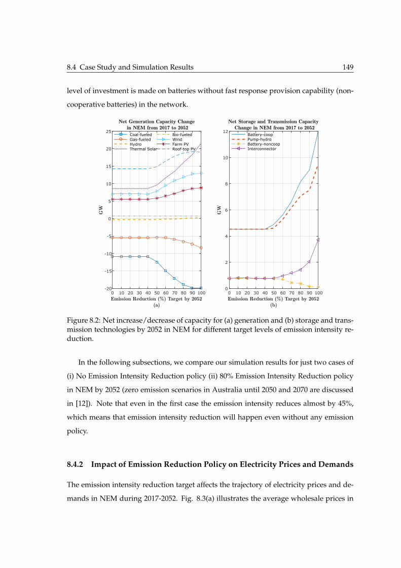
8.4 Case Study and Simulation Results 149
level of investment is made on batteries without fast response provision capability (non-
cooperative batteries) in the network.
Emission Reduction (%) Target by 2052(a)
0 10 20 30 40 50 60 70 80 90 100
GW
-20
-15
-10
-5
0
5
10
15
20
25
Net Generation Capacity Change in NEM from 2017 to 2052
Coal-fueledGas-fueledHydroThermal Solar
Bio-fueledWindFarm PVRoof-top PV
Emission Reduction (%) Target by 2052(b)
0 10 20 30 40 50 60 70 80 90 100
GW
0
2
4
6
8
10
12
Net Storage and Transmission Capacity Change in NEM from 2017 to 2052
Battery-coopPump-hydroBattery-noncoopInterconnector
Figure 8.2: Net increase/decrease of capacity for (a) generation and (b) storage and trans-mission technologies by 2052 in NEM for different target levels of emission intensity re-duction.
In the following subsections, we compare our simulation results for just two cases of
(i) No Emission Intensity Reduction policy (ii) 80% Emission Intensity Reduction policy
in NEM by 2052 (zero emission scenarios in Australia until 2050 and 2070 are discussed
in [12]). Note that even in the first case the emission intensity reduces almost by 45%,
which means that emission intensity reduction will happen even without any emission
policy.
8.4.2 Impact of Emission Reduction Policy on Electricity Prices and Demands
The emission intensity reduction target affects the trajectory of electricity prices and de-
mands in NEM during 2017-2052. Fig. 8.3(a) illustrates the average wholesale prices in

150 Designing Tax&Subsidy Incentives Towards a Green and Reliable Electricity Market
NEM by 2052 with and without implementing the emission reduction policy. It can be
seen that the market price is extremely high in 2017, which is the consequence of exercis-
ing market power by coal and gas generation firms. The price reduction trend continues
for the next twenty years, i.e., until 2037. In fact, investment on renewable technologies
increases the competition and reduces the prices for that period. By 2037, a large portion
of coal power plants are closed down in our model and the cost of installing new gen-
eration capacities rises the wholesale prices again during 2037-2052. Surprisingly, in the
price declining period, i.e., 2017-2037, imposing the emission intensity reduction policies
comparatively lowers the prices by 5%, which is related to the market power level. Pene-
tration of renewables increases the competition (reduces the market power) and leads to
lower prices.
Fig. 8.3(b) compares the average wholesale and net demand levels in NEM by 2052
with and without implementing the emission reduction policy. Note that the net demand
includes the roof-top PV generation in addition to the wholesale demand. The divergence
of the net and wholesale demand levels is caused by penetration of roof-top PVs in the
network. Roof-top PV generation increases by 3.93 times in No Emission Reduction Pol-
icy case and by 4.84 times in 80% Emission Reduction Policy case until 2052, which shows
that roof-top PV is competent enough to penetrate enormously by 2052 with or without
emission incentive policy.
8.4.3 Carbon Tax&Subsidy Design
We design the emission incentives based on the dual variable of the emission intensity
constraint, which is called carbon price, at the NE point in our model. Implementing
80% Emission Intensity Reduction policy, the emission intensity must uniformly decrease
from the base year level of 0.727 tonneCO2 /MWhe in 2017 to 0.145 tonneCO2 /MWhe in
2052. Fig. 8.4 (a) shows the calculated carbon price at different years to reach 80% emis-
sion intensity reduction by 2052. The carbon price moves upward in the beginning stage,
up to year 2032, then decreases during 2032-2042, and goes up again at the final stage,
2042-2052. The closure down of coal and gas power plants, which are at their end of life,
mostly happens during 2032-2042, which reduces the emission intensity and carbon price

8.4 Case Study and Simulation Results 151
year(a)
2017
2022
2027
2032
2037
2042
2047
2052
$/M
Wh
75
80
85
90
95
100
105
110
Mean Wholesale ElectricityPrice in NEM
Wholesale (No EI Reduction Policy)Wholesale (80% EI Reduction Policy)
year(b)
2017
2022
2027
2032
2037
2042
2047
2052
GW
22
24
26
28
30
32
34
36
Mean Wholesale&Net ElectricityDemand in NEM
Net (No EI Reduction Policy)Net (80% EI Reduction Policy)Wholesale (No EI Reduction Policy)Wholwsale (80% EI Reduction Policy)
Figure 8.3: The average yearly (a) wholesale prices and (b) net and wholesale demandsin NEM, without or with emission reduction policy (net demand =wholesale demand +roof-top PV).
level. However, higher levels of carbon price is calculated in our model to achieve higher
levels of emission intensity reduction at the final stage, regarding the uniform reduction
of emission intensity from 2017 to 2052.
Fig. 8.4 (b) indicates the average amounts of tax and subsidy that any type of gen-
erator pays or receives each year based on their electricity generation emission intensity
and the calculated carbon price of that year. As coal-fueled generators have emission
intensities much higher than the emission intensity target levels, they always pay carbon
tax in the market. The gas-fueled generators have lower emission intensities and do not
pay significant carbon penalty until 2042. The renewable generators, including wind, PV,
thermal solar, bio-fueled, and hydro, receive the carbon subsidy in the market, as their
generation emission intensity is zero. One kW capacity of thermal solar and bio-fueled
generators are more efficient in reducing the emission intensity than one kW of wind, PV
or even hydro, and thus receive higher emission subsidy in average.

152 Designing Tax&Subsidy Incentives Towards a Green and Reliable Electricity Market
year(a)
2022
2027
2032
2037
2042
2047
2052
$/to
nne
CO
2
0
20
40
60
80Carbon Price for 80% Emission Reduction Policy
year(b)
2022
2027
2032
2037
2042
2047
2052
$/kW
/yr
-100
0
100
200
300Mean Annual Carbon Tax&Subsidy for 80% Emission Reduction Policy
Coal-fueledGas-fueledWindPVThermal SolarBio-fueledHydro
Figure 8.4: The trajectory of (a) carbon price, (b) carbon tax (positive) and subsidy (nega-tive) of different generation types during 2017-2052.
8.4.4 Fast Response Capacity Tax&Subsidy Design
The other tax and subsidy incentive is calculated based on the dual variable of the fast
response dispatchable generation constraint at the NE point in our model. Intermittent
generators, i.e., wind and PV, are vulnerable to generation fluctuation due to wind and
solar energy availability. Therefore, there must be adequate fast response generation ca-
pacity to dispatch even out of merit, i.e., even when their marginal cost of generation
is above the market price, if wind or solar is lacking. As fast response generators may
dispatch out of merit, they need to be subsidized. The subsidy is provided by taxing the
intermittent generators. Fig. 8.5 indicates the level of fast response tax and subsidy for
different generation types during 2017-2052, with and without emission intensity reduc-
tion policy. It can be seen that implementing the emission reduction policy, which leads
to higher levels of intermittent generation in the market, we calculate higher amounts
of fast response tax and subsidy for all generators. Moreover, the subsidy level is not
the same for different generation types. One kW pump-hydro receives higher subsidy

8.4 Case Study and Simulation Results 153
for fast response provision than one kW battery as pump-hydros generally have larger
energy storage tanks (kWh). However, the battery’s fast response subsidy becomes more
than the pump-hydro’s in 2052 due to the decline in investment cost of the battery tanks.
The subsidy on hydro plants uniformly increases by time, but the subsidy on gas-fueled
plants increases significantly after 2042, as they have to pay considerable amounts of
emission tax at those times.
year(a)
2022
2027
2032
2037
2042
2047
2052
$/kW
/yr
-400
-300
-200
-100
0
100
Fast Response Capacity Tax&Subsidy without Emission Policy
WindPVBattery-coopPump-hydroHydroGas-fueled
year(b)
2022
2027
2032
2037
2042
2047
2052
$/kW
/yr
-400
-300
-200
-100
0
100
Fast Response Capacity Tax&Subsidy with 80% Emission Reduction Policy
Figure 8.5: The trajectory of fast response capacity tax (positive) and subsidy (negative)for (a) No Emission Reduction policy, (b) 80% Emission Intensity Reduction policy.
8.4.5 Impact of Market Power on Market Expansion
In this subsection, we compare our simulation results with the scenario when market
power is disregarded in the game, i.e., a perfectly competitive market. Fig. 8.6 illustrates
our simulation results for the generation, storage and transmission capacities in NEM
at the end of 2052 with and without market power consideration when there isn’t any
emission policy, Fig. 8.6(a), and when 80% emission intensity reduction policy is imple-
mented, Fig. 8.6(b). It can be seen that disregarding the market power, the investment on
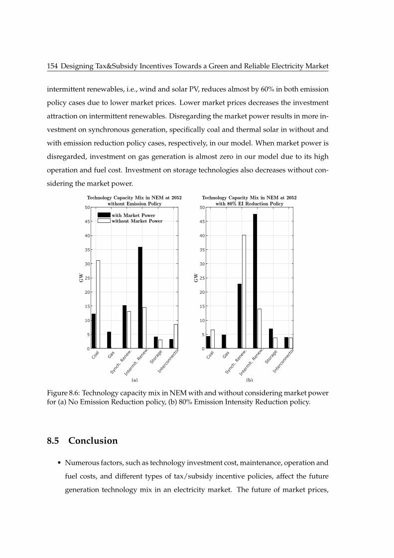
154 Designing Tax&Subsidy Incentives Towards a Green and Reliable Electricity Market
intermittent renewables, i.e., wind and solar PV, reduces almost by 60% in both emission
policy cases due to lower market prices. Lower market prices decreases the investment
attraction on intermittent renewables. Disregarding the market power results in more in-
vestment on synchronous generation, specifically coal and thermal solar in without and
with emission reduction policy cases, respectively, in our model. When market power is
disregarded, investment on gas generation is almost zero in our model due to its high
operation and fuel cost. Investment on storage technologies also decreases without con-
sidering the market power.
(a)
Coal
Gas
Sync
h. R
enew
.In
term
it. R
enew
.St
orag
eIn
terc
onne
ctor
GW
0
5
10
15
20
25
30
35
40
45
50
Technology Capacity Mix in NEM at 2052without Emission Policy
with Market Powerwithout Market Power
(b)
Coal
Gas
Sync
h. R
enew
.In
term
it. R
enew
.St
orag
eIn
terc
onne
ctor
GW
0
5
10
15
20
25
30
35
40
45
50
Technology Capacity Mix in NEM at 2052with 80% EI Reduction Policy
Figure 8.6: Technology capacity mix in NEM with and without considering market powerfor (a) No Emission Reduction policy, (b) 80% Emission Intensity Reduction policy.
8.5 Conclusion
• Numerous factors, such as technology investment cost, maintenance, operation and
fuel costs, and different types of tax/subsidy incentive policies, affect the future
generation technology mix in an electricity market. The future of market prices,

8.5 Conclusion 155
generation and demand levels are very sensitive to those factors. For instance, the
total capacity of non-cooperative batteries, which just make profit from energy ar-
bitrage, is much less than that of the cooperatively controlled batteries, which make
profit from both energy arbitrage and fast response service provision, despite hav-
ing similar investment costs.
• Emission intensity reduction policies do not necessarily increase the average elec-
tricity prices all the times. Considering the Emission Intensity Reduction policy
in our model, we calculated lower prices relative to No Emission Reduction pol-
icy scenario in the market until 2042. We also found that the price increase due to
implementing the emission policies after 2042 happens at off peak times and even
slightly reduces the peak time prices. This discussion is similar to the recent find-
ings in [68].
• Emission incentive policies, which are calculated based on the dual variable of the
emission constraint, can be used to penalize the pollutant generators and to re-
ward the renewables and clean technologies. It is observed in our simulations that
the retirement of the incumbent coal-fueled and gas-fueled generators reduces the
carbon price level and subsequently the emission incentive policy levels in 2042.
Thereafter, carbon price rises again to retain the emission intensity reduction trend
in the market.
• The incentive policies of fast response capacity tax and support, which are calcu-
lated based on the dual variable of the fast response generation constraint, can be
used to penalize the intermittent generators and subsidize the fast response capac-
ities. Gradual retirement of the incumbent gas-fueled plants and penetration of in-
termittent generators lead to higher levels of subsidy to ensure existence of enough
fast response capacity in the market.
• Considering the market power in a market expansion model significantly affects the
technology expansion decisions. Disregarding the market power, high electricity
prices are not calculated in the model, which does not provide enough incentive
for more recent technologies, like intermittent generators and batteries, to highly

156 Designing Tax&Subsidy Incentives Towards a Green and Reliable Electricity Market
penetrate in the market.
• The high level of investment on synchronous renewable capacity, like thermal so-
lar, which may have heat energy storage system or may be a hybrid system that
use other fuels during periods of low solar radiation, and battery storage can also
prevent the inertia and frequency response problems in electricity networks with
high level of intermittent generation, as discussed in [15].
In Chapter 9, we summarize the wholesale electricity market models we developed
in this thesis and highlight the important findings from this research as dot points.

Chapter 9
Conclusions
9.1 Summary of Chapters and Conclusions
IN THIS thesis, operational and planning Cournot-based wholesale electricity market
models are developed and used to analyze the supply, demand and price variations
in real-world electricity markets. Australia’s National Electricity Market is studied as the
case study, which is experiencing high levels of intermittent electricity generation and
price volatility in recent years. We extended the existing Cournot-based electricity market
models to analyze the price volatility in the market and find how storage can facilitate the
integration of renewable electricity in power networks. Moreover, we developed long-
term wholesale electricity market models to design tax and subsidy policies required to
achieve the emission and dispatchable capacity goals in the market.
In Chapter 2, a classic Cournot-based electricity market model including strategic
generation firms is introduced. The model is extended to consider storage and transmis-
sion players and states that:
• Strategic storage players maximize their profit from energy arbitrage and the strate-
gic transmission lines maximize their electricity trading profit based on the price
difference at their terminals.
• Any regulated generation, storage and transmission player maximizes the market
surplus or social welfare, which is the profit or surplus for both generators and
consumers, in our model.
• The defined game is developed as a centralized optimization problem to find the
157

158 Conclusions
NE solution as the game model just includes linear inverse demand functions.
In Chapter 3, we briefly introduce the National Electricity Market in Australia and ex-
plain its pricing mechanism. Then we compare the linear and non-linear inverse demand
functions and show that
• Accurate calibration of the inverse demand functions reduces our simulation error
terms (comparing to historical price and demand data).
In Chapter 4, a multi-region Cournot-based electricity market model with nonlin-
ear inverse demand functions is developed, which is solved as a Mixed Complementary
Problem. The transmission lines are modeled as individual market players likewise the
other firms in the game, which leads to far more convenient computations than when the
transmission lines are considered as constraints for a market clearing engine. The model
is applied to the 5-node NEM market, and is calibrated with realistic data from year
2015. The market is simulated with and without considering a large coal power plant
in the game under 365 intermittent energy availability scenarios to find how a base-load
power plant closure impacts the market price and volatility. Our simulations in the NEM
market show:
• The highest proportional change in average price, peak price and price volatility
happens in the region (VIC) where the closure happens and then in its neighboring
regions TAS and SA.
• Depending on the capacity of interconnectors, the impact of coal plant closure may
differ in different market regions.
• The aggregate CO2 emission of gas and coal power plants in the market, which is
affected by the electricity market prices, reduces by 5.8% after the coal power plant
closure.
In Chapter 5, a bi-level optimization model is proposed to find the minimum storage
capacity required to achieve a price volatility level in an electricity market. In the upper
level problem, the optimal regional storage capacities are found, and in the lower level
9.1 Summary of Chapters and Conclusions 159
problem, the Bayes-NE solution of the market under a set of scenarios is calculated. The
non-cooperative interaction between regulated/strategic generation, storage and trans-
mission players in the market is calculated using a stochastic Cournot-based game with
a non-linear inverse demand function. The exponential inverse demand function is ac-
curate enough to model the impact of storage on reducing the very high prices in the
market. The existence of Bayes-NE is established for the lower level problem under the
exponential inverse demand function. The bi-level problem is converted into a single
level problem as a MPEC and is solved by a greedy algorithm. The simulation results in
the NEM market show that:
• Storage alleviates the price volatility but does not remove it completely.
• Regulated storage firms are more efficient in reducing the price volatility than strate-
gic storage firms.
• Although both storage and transmission capacities are able to reduce the price
volatility level in the market, regulated storage can effectively alleviate high lev-
els of price volatility when transmission lines are under maintenance.
• As a rule of thumb, a region with highest share of intermittent electricity in its total
generation is the candidate to install storage capacity to reduce the price volatility
in a multi-region electricity market.
In Chapter 6, a bi-level optimization model is proposed to allocate a fixed budget on
regulated storage and wind capacities in order to minimize the weighted sum of average
price and price volatility in a single region taking into account the interdependency be-
tween different regions. In the upper level problem, the weighted sum of average price
and price volatility is minimized by allocating a budget on regulated wind and storage
capacities in the specified region. In the lower level problem, a stochastic Cournot-based
electricity market model with non-linear inverse demand functions is used to model the
non-cooperative interaction between regulated/strategic generation, storage and trans-
mission firms. The bi-level problem is converted into a single-level problem as a MPEC
and is solved by a line-search algorithm. Based on our simulations, in the NEM market:

160 Conclusions
• Both storage and wind are capable of reducing the average price and price volatility,
but storage is more efficient in reducing the price volatility and wind in reducing
the average price.
• Based on the importance of average price and volatility, a mixed combination of
storage and wind can optimally minimize the weighted sum of price and volatility
in the market.
• Wind turbine is almost a mature generation technology and is competent enough
to penetrate in the market in large scales.
• The future reduction in investment cost of battery storage also enables this technol-
ogy to penetrate economically in the market in large scales.
In Chapter 7, a long-term stochastic Cournot-based generation expansion model with
a carbon cap constraint is developed which considers a set of scenarios due to wind
power intermittency. Generation players decide on their long-term capacity addition and
retirement as well as their operation in our model considering a carbon cap constraint in
the market. The dual variable of the carbon cap constraint at the Bayes-NE point is used
to calculate the carbon price in the market. The game model includes linear inverse de-
mand functions and is solved as a centralized optimization problem. The simulation
results, in a generic electricity market with three generation firms of coal, gas and wind,
show that:
• Carbon cap constraint leads to proportionally more renewable and less fossil-fueled
generation capacity in the market.
• Higher tax on carbon emission is required to install renewables when they are
highly stochastic.
• The higher levels of carbon tax can be spent on adding storage technologies to en-
counter intermittency in renewable generation.
• Comparing the strategic and perfectly competitive behaviors for the wind firm, we
observe that the coal firm adds more capacity and the gas firm slightly decreases
9.2 Future Research 161
its new capacity decisions when wind player strategically reduces its new capacity
investment plan.
In Chapter 8, a long-term Cournot-based market expansion model with emission in-
tensity reduction and fast response dispatchable capacity constraints is developed. The
regulated/strategic generation, storage and transmission players decide on their long
term capacity expansion and their operation in the model considering the emission in-
tensity and fast response capacity constraints. Based on the KKT equations of the game,
it is explained how dual variables of the emission and fast capacity constraints at the NE
point is used to calculate the tax and subsidy policies required to achieve the emission
and reliability goals in the market. The simulation results, in the NEM market, shows
that:
• Setting emission reduction policies does not necessarily lead to higher prices and
even may decrease the electricity prices at peak hours.
• The incentive policies of fast response capacity can ensure existence of enough dis-
patchable capacity to balance the supply and demand at any time in the market.
• Considering the market power in expansion models leads to high electricity prices
and more investment on expensive technologies in the market.
9.2 Future Research
We used the availability factor for any technology in our developed models to consider
the maintenance of power plants, storage technologies and transmission lines in our cal-
culations. The availability factor indicates that the corresponding technology is not avail-
able during its maintenance time. However, power plants may make strategic mainte-
nance decisions, which can impact the market prices significantly. In future works, the
impact of strategic maintenance decisions [22] of power-plants on market prices, espe-
cially when a coal plant is closed down, can be studied.
Furthermore, our proposed storage allocation model can be extended by considering
the ancillary services and capacity markets. The impact of ancillary service markets [21]

162 Conclusions
and capacity markets [23] on the integration of storage systems in electricity networks
is left as an open problem. It is also interesting to study the wind correlation analysis
to look at volatility reduction effectiveness in future works. Moreover, future research
can include the optimal storage siting problem subject to the line congestion constraint
to alleviate the congestion problem.
Although we did not discuss the ancillary service markets in our electricity market
models, Cournot-based models are able to find the value of any ancillary services that
are provided in the market. For instance, considering a constraint on minimum electric-
ity supply in the market, one can find the value of providing the minimum level of elec-
tricity generation at all times in the market. Using the dual value of the minimum supply
constraint at the NE point, it can be calculated that how much must be paid to generators
in order to provide the minimum electricity supply service in the market. Moreover, con-
sidering a constraint on the existence of reserve capacity in the market, one can calculate
the value of reserve capacity based on the dual variable of the constraint at the NE point.
Finally, in our developed electricity market models in this thesis, consumers (retailers)
are all considered as price taker players, i.e., perfectly competitive firms. However, if a
large retailer with load curtailment ability exists in an electricity market, it possesses
market power on the demand side and bids strategically to reduce the price. Existence
of market power on the demand side may have a counter effect on the exercise of market
power on the supply side and may make the market more competitive. To the best of our
knowledge, the strategic behavior of consumers in a wholesale electricity markets, i.e., in
two sided electricity markets, remains an open problem.

Appendix A
Charging/Discharging
In this appendix, we show that the charge and discharge levels of any storage device
cannot be simultaneously positive at the NE of the lower level game under each scenario
in Chapters 5 and 6. Consider a strategy in which both charge and discharge levels of
storage device i at time t under scenario w, i.e. qdisitw, qch
itw, are both positive. We show that
this strategy cannot be a NE strategy of scenario w as follows. The net electricity flow of
storage can be written as qstitw = ηdis
i qdisitw −
qchitw
ηchi
. Let qdisitw and qch
itw be the new discharge and
charge levels of storage firm i defined as
qdisitw = qdis
itw −qch
itwηdis
i ηchi
, qchitw = 0
if qst
itw > 0, orqdis
itw = 0, qchitw = qch
itw − qdisitwηdis
i ηchi
if qst
itw < 0. The new net flow of electricity can be
written as qstitw = ηdis
i qdisitw −
qchitw
ηchi
. Note that the new variables qstitw, qch
itw and qdisitw satisfy the
constraints (5.5a-5.5d).
Considering the new charge and discharge strategies qdisitw and qch
itw, instead of qdisitw and
qchitw, the nodal price and the net flow of storage device i do not change. However, the
charge/discharge cost of the storage firm i, under the new strategy, is reduces by:
csti
(qch
itw + qdisitw
)− cst
i
(qdis
itw + qchitw
)> 0
Hence, any strategy at each scenario in which the charge and discharge variables are
simultaneously positive cannot be a NE, i.e. at the NE of the lower game under each
scenario each storage firm is either in the charge mode or discharge mode.
163


Appendix B
Regulated Transmission Firms
In this appendix, we show how the objective function of any transmission player in Chap-
ter 6 is generalized to be either strategic (profit maximizer) or regulated (social welfare
maximizer). When γtrij in (6.9a) is zero, the player maximizes its profit and when γtr
ij is
one, the player equivalently maximizes the social welfare (SW). The definition of social
welfare, under any scenario w in our problem, is the total surplus of consumers and pro-
ducers as:
SWw = ∑i,t
∫ yitw
0Pitw (.) ∂yitw − Total Costsit
= ∑i,t
Pitw (.)− αit
−βit− Total Costit
where Total Cost is the total cost of electricity generation, storage, and transmission.
The derivative of the social welfare function respect to qtrijtw, given the constraint
(6.9b), that is, qtrijtw = −qtr
jitw, is:
∂SWw
∂qtrijtw
= Pitw (.)− Pjtw (.) ,
and the derivative of regulated term in (6.9a) respect to qtrijtw is:
∂(
Pjtw(.)−β jt
+ Pitw(.)−βit
)∂qtr
ijtw= Pitw (.)− Pjtw (.)
165

166 Regulated Transmission Firms
which shows that based on the first order optimality conditions, maximizing the regu-
lated term is equivalent to maximizing the social welfare for the transmission player.

Appendix C
Technology Characteristics
All financial and technical information on intermittent and synchronous generators, stor-
age technologies and Interconnectors are from [12, 54, 97] in Chapter 8.
Table C.1: Financial and Technical Information on Intermittent Generators in NEM.
GeneratorType:
windTurbine
FarmPV
Roof-topPV
Qig2017 (GW) 3.733 0.356 4.826˜Invig ( $
kW )(a),(b)
2400(1.5%) 2190(3.5%) 2100(3.5%)
cig ( $MWh ) 5 2 2
dig ($
MWhMWh ) 0.00125 0.00125 0
PLig (yr) 25 20 20Cig (GW) n.a n.a 24.266
(a) Yearly maintenance cost is approximated by 1 percent of investment cost for all generation, storageand transmission technologies in our calculations.(b) Investment cost de-escalator rate (%). After 2037 the de-escalator used for wind and all the differentsolar technologies drops to 0.3% since they are considered mature technologies.
167

168 Technology Characteristics
Table C.2: Financial and Technical Information on Synchronous Generators in NEM.
Plant: Qsg2017
(GW)˜Invsg
( $kW )(a)
csg ( $MWh )
operation+ fuel
PLsg
(yr)Rup,Rdn
( %hr , %
hr )
Asg
(%)EF(
tCO2MWh )
RAsg
( TWhyr )
αsg,FR
∈0, 1
Black Coal 18.440 4285(0.1%) 3+18 50 10 75 1 n.a 0Brown Coal 4.730 5715(0.1%) 3+16.5 50 10 75 1.2 n.a 0Thermal Gas 1.837 1910(0.2%) 7.5+84 30 10 75 0.62 n.a 0CC Gas Turbine 3.402 2100(0.2%) 6.1+56 30 10 75 0.41 n.a 0OC Gas Turbine 6.076 1720(0.2%) 9+84 30 100 75 0.62 n.a 1Solar Thermalwith Storage
0 8500(2.5%) 25+0 35 10 75 0 n.a 0
Biomass 1.014 6500(0.5%) 8+42 30 10 75 0 7.8 0Hydro 5.711 3600(0.5%) 5+0 35 100 70 0 23.96 1
(a) Capital cost de-escalator rate (%). After 2037 the de-escalator used for solar thermal drops to 0.3%.
Table C.3: Financial and Technical Information on Storage Technologies in NEM.
Storage Type: Pump-hydro
Cooperativebattery
Non-cooperativebattery
Qst,f2017 (GW) 2160 0 0
Qst,v2017 (GWh) 21600 0 0˜Invst,f ( $
kW )(a) 800(0.5%) 225(3.1%) 150(3.1%)
˜Invst,v ( $kWh ) 70(0.5%) 225(3.1%) 225(3.1%)
PLst,f (yr) 30 10 10PLst,v (yr) 50 10 10ηdis,ηch (%,%) 85,85 95,95 95,95Ast (%) 70 90 90αsg,FR ∈ 0, 1 1 1 0
(a) Investment cost de-escalator rate (%).
Table C.4: Financial and Technical Information on Interconnectors in NEM.
Interconnector: SA-VIC
TAS-VIC
VIC-NSW
QLD-NSW
Qtr2017 (GW)
Forward510 478 150 800
Qtr2017 (GW)
Reverse680 594 500 1400
˜Invtr ( $kW ) 1000 1600 700 1100
PLtr (yr) 50 50 50 50ηtr (%) 95 95 95 95Atr (%) 70 70 70 70

Bibliography
[1] A. G. Kagiannas, D. T. Askounis, and J. Psarras, “Power generation planning: a
survey from monopoly to competition,” International Journal of Electrical Power &
Energy Systems, pp. 413–421, 2004.
[2] IEA, “Technology Roadmap, Hydro Power,” International Energy Agency, Tech.
Rep., 2012.
[3] H. Lund and B. Mathiesen, “Energy system analysis of 100% renewable energy
systems-The case of Denmark in years 2030 and 2050 ,” Energy, vol. 34, no. 5, pp.
524 – 531, 2009.
[4] J. C. Ketterer, “The impact of wind power generation on the electricity price in Ger-
many,” Energy Economics, vol. 44, pp. 270–280, 2014.
[5] D. Wozabal, C. Graf, and D. Hirschmann, “The effect of intermittent renewables on
the electricity price variance,” OR spectrum, pp. 1–23, 2014.
[6] C.-K. Woo, I. Horowitz, J. Moore, and A. Pacheco, “The impact of wind generation
on the electricity spot-market price level and variance: The Texas experience,” En-
ergy Policy, vol. 39, no. 7, pp. 3939–3944, 2011.
[7] D. Chattopadhyay and T. Alpcan, “A Game-Theoretic Analysis of Wind Generation
Variability on Electricity Markets,” Power Systems, IEEE Transactions on, vol. 29, no. 5,
pp. 2069–2077, Sept 2014.
[8] S.-J. Deng and S. S. Oren, “Electricity derivatives and risk management,” Energy,
vol. 31, no. 6, pp. 940–953, 2006.
169

170 BIBLIOGRAPHY
[9] H. Higgs and A. Worthington, “Stochastic price modeling of high volatility, mean-
reverting, spike-prone commodities: The Australian wholesale spot electricity mar-
ket,” Energy Economics, vol. 30, p. 31723185, 2008.
[10] A. Tishler, I. Milstein, and C.-K. Woo, “Capacity commitment and price volatility in
a competitive electricity market,” Energy Economics, vol. 30, no. 4, pp. 1625 – 1647,
2008.
[11] P. Williams, “Power Price Spike Hits Australia as Coal Plant Shuts Down,” March
2017. [Online]. Available: www.bloomberg.com/news
[12] W. Gerardi and P. Galanis, “Emissions mitigation policies and security of electricity
supply,” Jacobs Group (Australia), Tech. Rep., June 2017.
[13] S. Borenstein, “Understanding competitive pricing and market power in wholesale
electricity markets,” The Electricity Journal, vol. 13, no. 6, pp. 49 – 57, 2000.
[14] “Paris Agreement,” United Nations Treaty Collection, 8 July 2016.
[15] P. Mancarella, “Power system security assessment of the future National Electricity
Market,” Melbourne Energy Institute, Tech. Rep., 2017.
[16] X. Hu, G. Grozev, and D. Batten, “Empirical observations of bidding patterns in
Australias National Electricity Market,” Energy Policy, vol. 33, p. 20752086, 2005.
[17] R. Loulou, U. Remne, A. Kanudia, A. Lehtila, and G. Goldstein, “Documentation for
the TIMES Model PART I,” Energy Technology Systems Analysis Programme, Tech.
Rep., 2005.
[18] W. Jing-Yuan and Y. Smeers, “Spatial Oligopolistic Electricity Models with Cournot
Generators and Regulated Transmission Prices,” Operations Research, vol. 47, no. 1,
pp. 102–112, 1999.
[19] D. Chattopadhyay, “Modeling Greenhouse Gas Reduction From the Australian Elec-
tricity Sector,” Power Systems, IEEE Transactions on, vol. 25, no. 2, pp. 729–740, May
2010.

BIBLIOGRAPHY 171
[20] W. W. Hogan, “A Market Power Model with Strategic Interaction in Electricity Net-
works,” The Energy Journal, vol. 18, no. 4, pp. 107–141, 1997.
[21] D. Chattopadhyay, “Multicommodity spatial Cournot model for generator bidding
analysis,” Power Systems, IEEE Transactions on, vol. 19, no. 1, pp. 267–275, Feb 2004.
[22] ——, “A game theoretic model for strategic maintenance and dispatch decisions,”
Power Systems, IEEE Transactions on, vol. 19, no. 4, pp. 2014–2021, Nov 2004.
[23] D. Chattopadhyay and T. Alpcan, “Capacity and Energy-Only Markets Under High
Renewable Penetration,” Power Systems, IEEE Transactions on, vol. PP, no. 99, pp.
1–11, 2015.
[24] W.-P. Schill, C. Kemfert et al., “Modeling strategic electricity storage: the case of
pumped hydro storage in Germany,” Energy Journal-Cleveland, vol. 32, no. 3, p. 59,
2011.
[25] J. de Hoog, T. Alpcan, M. Brazil, D. Thomas, and I. Mareels, “Optimal Charging
of Electric Vehicles Taking Distribution Network Constraints Into Account,” Power
Systems, IEEE Transactions on, vol. 30, no. 1, pp. 365–375, Jan 2015.
[26] W. Saad, Z. Han, H. Poor, and T. Basar, “A noncooperative game for double auction-
based energy trading between PHEVs and distribution grids,” in Smart Grid Com-
munications (SmartGridComm), 2011 IEEE International Conference on, Oct 2011, pp.
267–272.
[27] N. Lu, J. Chow, and A. Desrochers, “Pumped-storage hydro-turbine bidding strate-
gies in a competitive electricity market,” Power Systems, IEEE Transactions on, vol. 19,
no. 2, pp. 834–841, May 2004.
[28] A. Masoumzadeh, D. Most, and S. C. Ookouomi Noutchie, “Partial equilibrium
modelling of world crude oil demand, supply and price,” Energy Systems, pp. 1–10,
2016.
172 BIBLIOGRAPHY
[29] M. Ventosa, R. Denis, and C. Redondo, “Expansion planning in electricity markets.
Two different approaches,” in Proceedings of the 14th Power Systems Computation Con-
ference (PSCC), Seville, 2002.
[30] B. E. Hobbs, “Linear complementarity models of Nash-Cournot competition in bi-
lateral and POOLCO power markets,” IEEE Transactions on Power Systems, vol. 16,
no. 2, pp. 194–202, May 2001.
[31] J. B. Cardell, C. C. Hitt, and W. W. Hogan, “Market power and strategic interaction
in electricity networks ,” Resource and Energy Economics, vol. 19, no. 12, pp. 109 – 137,
1997.
[32] S. Wogrin, E. Centeno, and J. Barquin, “Generation capacity expansion in liberal-
ized electricity markets: A stochastic MPEC approach,” IEEE Transactions on Power
Systems, vol. 26, no. 4, pp. 2526–2532, Nov 2011.
[33] A. Masoumzadeh, E. Nekouei, and T. Alpcan, “Long-term stochastic planning in
electricity markets under carbon cap constraint: A Bayesian game approach,” in
2016 IEEE Innovative Smart Grid Technologies - Asia (ISGT-Asia), Nov 2016, pp. 466–
471.
[34] B. Hobbs, C. Metzler, and J.-S. Pang, “Strategic gaming analysis for electric power
systems: an MPEC approach,” Power Systems, IEEE Transactions on, vol. 15, no. 2, pp.
638–645, May 2000.
[35] E. G. Kardakos, C. K. Simoglou, and A. G. Bakirtzis, “Optimal bidding strategy in
transmission-constrained electricity markets ,” Electric Power Systems Research, vol.
109, pp. 141 – 149, 2014.
[36] S. J. Kazempour and H. Zareipour, “Equilibria in an Oligopolistic Market With Wind
Power Production,” IEEE Transactions on Power Systems, vol. 29, no. 2, pp. 686–697,
March 2014.

BIBLIOGRAPHY 173
[37] N. Li, C. Ukun, E. M. Constantinescu, J. R. Birge, K. W. Hedman, and A. Botterud,
“Flexible Operation of Batteries in Power System Scheduling With Renewable En-
ergy,” IEEE Transactions on Sustainable Energy, vol. 7, no. 2, pp. 685–696, April 2016.
[38] V. Krishnan and T. Das, “Optimal allocation of energy storage in a co-optimized
electricity market: Benefits assessment and deriving indicators for economic storage
ventures ,” Energy, vol. 81, pp. 175 – 188, 2015.
[39] A. Berrada and K. Loudiyi, “Operation, sizing, and economic evaluation of storage
for solar and wind power plants ,” Renewable and Sustainable Energy Reviews, vol. 59,
pp. 1117 – 1129, 2016.
[40] W. Qi, Y. Liang, and Z.-J. M. Shen, “Joint Planning of Energy Storage and Transmis-
sion for Wind Energy Generation,” Operations Research, vol. 63, no. 6, pp. 1280–1293,
2015.
[41] M. Sedghi, A. Ahmadian, and M. Aliakbar-Golkar, “Optimal Storage Planning in
Active Distribution Network Considering Uncertainty of Wind Power Distributed
Generation,” IEEE Transactions on Power Systems, vol. 31, no. 1, pp. 304–316, Jan 2016.
[42] L. Zheng, W. Hu, Q. Lu, and Y. Min, “Optimal energy storage system allocation
and operation for improving wind power penetration,” IET Generation, Transmission
Distribution, vol. 9, no. 16, pp. 2672–2678, 2015.
[43] J. Xiao, Z. Zhang, L. Bai, and H. Liang, “Determination of the optimal installation
site and capacity of battery energy storage system in distribution network integrated
with distributed generation,” IET Generation, Transmission Distribution, vol. 10, no. 3,
pp. 601–607, 2016.
[44] Y. Zheng, Z. Y. Dong, F. J. Luo, K. Meng, J. Qiu, and K. P. Wong, “Optimal Alloca-
tion of Energy Storage System for Risk Mitigation of DISCOs With High Renewable
Penetrations,” IEEE Transactions on Power Systems, vol. 29, no. 1, pp. 212–220, Jan
2014.

174 BIBLIOGRAPHY
[45] R. Walawalkar, J. Apt, and R. Mancini, “Economics of electric energy storage for
energy arbitrage and regulation in New York ,” Energy Policy, vol. 35, no. 4, pp. 2558
– 2568, 2007.
[46] H. Mohsenian-Rad, “Optimal Bidding, Scheduling, and Deployment of Battery Sys-
tems in California Day-Ahead Energy Market,” IEEE Transactions on Power Systems,
vol. 31, no. 1, pp. 442–453, Jan 2016.
[47] H. Akhavan-Hejazi and H. Mohsenian-Rad, “A stochastic programming framework
for optimal storage bidding in energy and reserve markets,” in Innovative Smart Grid
Technologies (ISGT), 2013 IEEE PES, Feb 2013, pp. 1–6.
[48] H. Mohsenian-Rad, “Coordinated Price-Maker Operation of Large Energy Storage
Units in Nodal Energy Markets,” IEEE Transactions on Power Systems, vol. 31, no. 1,
pp. 786–797, Jan 2016.
[49] E. Nasrolahpour, S. J. Kazempour, H. Zareipour, and W. D. Rosehart, “Strategic Siz-
ing of Energy Storage Facilities in Electricity Markets,” IEEE Transactions on Sustain-
able Energy, vol. 7, no. 4, pp. 1462–1472, Oct 2016.
[50] X. Fang, F. Li, Y. Wei, and H. Cui, “Strategic scheduling of energy storage for load
serving entities in locational marginal pricing market,” IET Generation, Transmission
Distribution, vol. 10, no. 5, pp. 1258–1267, 2016.
[51] A. Awad, J. Fuller, T. EL-Fouly, and M. Salama, “Impact of Energy Storage Systems
on Electricity Market Equilibrium,” Sustainable Energy, IEEE Transactions on, vol. 5,
no. 3, pp. 875–885, July 2014.
[52] A. Masoumzadeh, E. Nekouei, T. Alpcan, and D. Chattopadhyay, “Impact of Opti-
mal Storage Allocation on Price Volatility in Energy-only Electricity Markets,” IEEE
Transactions on Power Systems, vol. PP, no. 99, pp. 1–1, 2017.
[53] A. Masoumzadeh, H. Rasekhi, and A. Fathi, “A comprehensive energy supply
model in an office building based on the reference energy system,” International Jour-
nal of Sustainable Energy, vol. 35, no. 1, pp. 88–102, 2016.

BIBLIOGRAPHY 175
[54] M. Jeppesen, M. Brear, D. Chattopadhyay, C. Manzie, R. Dargaville, and T. Alpcan,
“Least cost, utility scale abatement from Australia’s NEM (National Electricity Mar-
ket). Part 1: Problem formulation and modelling,” Energy, vol. 101, pp. 606 – 620,
2016.
[55] W. El-Khattam, K. Bhattacharya, Y. Hegazy, and M. M. A. Salama, “Optimal invest-
ment planning for distributed generation in a competitive electricity market,” IEEE
Transactions on Power Systems, vol. 19, no. 3, pp. 1674–1684, Aug 2004.
[56] A. S. Chuang, F. Wu, and P. Varaiya, “A game-theoretic model for generation expan-
sion planning: problem formulation and numerical comparisons,” IEEE Transactions
on Power Systems, vol. 16, no. 4, pp. 885–891, Nov 2001.
[57] L. Wang, M. Mazumdar, M. D. Bailey, and J. Valenzuela, “Oligopoly models for
market price of electricity under demand uncertainty and unit reliability,” European
Journal of Operational Research, vol. 181, no. 3, pp. 1309 – 1321, 2007.
[58] J. Sirikum, A. Techanitisawad, and V. Kachitvichyanukul, “A New Efficient GA-
Benders’ Decomposition Method: For Power Generation Expansion Planning With
Emission Controls,” IEEE Transactions on Power Systems, vol. 22, no. 3, pp. 1092–1100,
Aug 2007.
[59] C. Unsihuay-Vila, J. W. Marangon-Lima, A. C. Z. de Souza, I. J. Perez-Arriaga, and
P. P. Balestrassi, “A Model to Long-Term, Multiarea, Multistage, and Integrated
Expansion Planning of Electricity and Natural Gas Systems,” IEEE Transactions on
Power Systems, vol. 25, no. 2, pp. 1154–1168, 2010.
[60] H. Mirzaesmaeeli, A. Elkamel, P. Douglas, E. Croiset, and M. Gupta, “A multi-
period optimization model for energy planning with CO2 emission consideration,”
Journal of Environmental Management, vol. 91, no. 5, pp. 1063 – 1070, 2010.
[61] J. Santisirisomboon, B. Limmeechokchai, and S. Chungpaibulpatana, “Impacts of
biomass power generation and CO2 taxation on electricity generation expansion
planning and environmental emissions,” Energy Policy, vol. 29, no. 12, pp. 975 –
985, 2001.

176 BIBLIOGRAPHY
[62] I. Das, K. Bhattacharya, and C. Caizares, “Optimal Incentive Design for Targeted
Penetration of Renewable Energy Sources,” IEEE Transactions on Sustainable Energy,
vol. 5, no. 4, pp. 1213–1225, 2014.
[63] Y. Zhou, L. Wang, and J. D. McCalley, “Designing effective and efficient incentive
policies for renewable energy in generation expansion planning,” Applied Energy,
vol. 88, no. 6, pp. 2201 – 2209, 2011.
[64] H. Almutairi and S. Elhedhli, “Carbon tax based on the emission factor: a bilevel
programming approach,” Journal of Global Optimization, vol. 58, no. 4, pp. 795–815,
2014.
[65] F. H. Murphy and Y. Smeers, “Generation Capacity Expansion in Imperfectly Com-
petitive Restructured Electricity Markets,” Operations Research, vol. 53, no. 4, pp.
646–661, 2005.
[66] I. Milstein and A. Tishler, “Intermittently renewable energy, optimal capacity mix
and prices in a deregulated electricity market,” Energy Policy, vol. 39, no. 7, pp. 3922
– 3927, 2011, special Section: Renewable energy policy and development.
[67] X. Zhou, G. James, A. Liebman, Z. Y. Dong, and C. Ziser, “Partial Carbon Permits
Allocation of Potential Emission Trading Scheme in Australian Electricity Market,”
IEEE Transactions on Power Systems, vol. 25, no. 1, pp. 543–553, 2010.
[68] A. Finkel, “The Independent Review into the Future Security of the National Elec-
tricity Market: Blueprint for the Future,” Commonwealth of Australia, Tech. Rep.,
2017.
[69] F. Leuthold, H. Weigt, and C. von Hirschhausen, “A Model of the European Electric-
ity Market,” Chair for Energy Economics and Public Sector Management, Dresden
University of Technology, Tech. Rep., 2008.
[70] D. P. Bertsekas, Nonlinear Programming, 2nd ed. Athena Scientific, 1999.
[71] T. Basar and G. Olsder, Dynamic Noncooperative Game Theory, 2nd Edition. Society
for Industrial and Applied Mathematics, 1998.

BIBLIOGRAPHY 177
[72] E. Nekouei, T. Alpcan, and M. Brandao, “Controlling multiple batteries on a radial
line,” in Power Engineering Conference (AUPEC), 2014 Australasian Universities, Sept
2014, pp. 1–7.
[73] M. C. Ferris and T. S. Munson, “GAMS/PATH user guide: Version 4.3,” Washington,
DC: GAMS Development Corporation, 2000.
[74] M. P. Moghaddam, A. Abdollahi, and M. Rashidinejad, “Flexible demand response
programs modeling in competitive electricity markets,” Applied Energy, vol. 88, no. 9,
pp. 3257–3269, 2011.
[75] P. Graham, S. Thorpe, and L. Hogan, “Non-competitive market behaviour in the
international coking coal market ,” Energy Economics, vol. 21, no. 3, pp. 195 – 212,
1999.
[76] D. Kirschen, G. Strbac, P. Cumperayot, and D. de Paiva Mendes, “Factoring the elas-
ticity of demand in electricity prices,” Power Systems, IEEE Transactions on, vol. 15,
no. 2, pp. 612–617, May 2000.
[77] S. A. Gabriel, A. J. Conejo, J. D. Fuller, B. F. Hobbs, and C. Ruiz, Complementarity
modeling in energy markets. Springer Science & Business Media, 2012, vol. 180.
[78] AEMO, “An Introduction to Australia’s National Electricity Market,” Australian En-
ergy Market Operator, Tech. Rep., 2010.
[79] D. Fudenberg and J. Tirole, Game theory. Cambridge, Mass. : M.I.T. Press, 1991.
[80] J. M. Morales, S. Pineda, A. J. Conejo, and M. Carrion, “Scenario reduction for
futures market trading in electricity markets,” IEEE Transactions on Power Systems,
vol. 24, no. 2, pp. 878–888, 2009.
[81] J. C. Harsanyi, “Games with Incomplete Information Played by ”Bayesian” Players,
I-III. Part II. Bayesian Equilibrium Points,” Management Science, vol. 14, no. 5, pp.
320–334, 1968.
[82] AEMC, “Potential Generator Market Power in the NEM,” Australian Energy Market
Commission, Tech. Rep. ERC0123, 26 April 2013.

178 BIBLIOGRAPHY
[83] G. Kirchgassner and J. Wolters, Introduction to modern time series analysis. Springer
Science & Business Media, 2007.
[84] X. Fang, F. Li, Q. Hu, and Y. Wei, “Strategic CBDR bidding considering FTR and
wind power,” IET Generation, Transmission Distribution, vol. 10, no. 10, pp. 2464–
2474, 2016.
[85] M. J. Neely, A. S. Tehrani, and A. G. Dimakis, “Efficient algorithms for renewable en-
ergy allocation to delay tolerant consumers,” in Smart Grid Communications (Smart-
GridComm), 2010 First IEEE International Conference on. IEEE, 2010, pp. 549–554.
[86] M. C. Ferris and T. S. Munson, “Complementarity problems in GAMS and the PATH
solver,” Journal of Economic Dynamics and Control, vol. 24, no. 2, pp. 165–188, 2000.
[87] Frontier-Economics, “Generator Nodal Pricing–a review of theory and practical ap-
plication,” Frontier Economics Pty Ltd., Melbourne, Tech. Rep., 2008.
[88] AER, “State Of The Energy Market 2015,” Australian Energy Regulator, Tech. Rep.,
2015.
[89] AEMO, “Roof-top PV Information Paper, National Electricity Forecasting,” Aus-
tralian Energy Market Operator, Tech. Rep., 2012.
[90] O. Alsac and B. Stott, “Optimal load flow with steady-state security,” IEEE transac-
tions on power apparatus and systems, no. 3, pp. 745–751, 1974.
[91] A. Masoumzadeh, E. Nekouei, and T. Alpcan, “Impact of a coal power plant closure
on a multi-region wholesale electricity market,” in 2017 IEEE PES Innovative Smart
Grid Technologies Conference Europe (ISGT-Europe), Sept 2017, pp. 1–6.
[92] C. S. Park, G. Kim, and S. Choi, Engineering economics. Prentice Hall: Upper Saddle
River, NJ, USA, 2007, vol. 22.
[93] Y. Saboohi, “Energy Supply Model: ESM 84,” Sharif Energy Research Institute
(SERI), Tech. Rep., 2005.

BIBLIOGRAPHY 179
[94] EIA, “Updated Capital Cost Estimates for Utility Scale Electricity Generation
Plants,” U.S. Department of Energy, Tech. Rep., April 2013.
[95] A. S. Drud, “CONOPT A Large-Scale GRG Code,” ORSA Journal on Computing 6, p.
207216, 1992.
[96] A. Niklaus and L. Dowling, “Renewables Influence on the Generation Mix and Gas
Demand in Western Australia,” Australian Energy Market Operator, Tech. Rep.,
May 2017.
[97] NERA, “Wholesale Electricity Costs in the NEM; A Report for the Australian Energy
Market Commission,” NERA Economic Consulting, Tech. Rep., August 2013.

Minerva Access is the Institutional Repository of The University of Melbourne
Author/s:Masoumzadeh, Amin
Title:Game-theoretic analysis of Australia's national electricity market (NEM) under renewablesand storage integration
Date:2018
Persistent Link:http://hdl.handle.net/11343/213868
Terms and Conditions:Terms and Conditions: Copyright in works deposited in Minerva Access is retained by thecopyright owner. The work may not be altered without permission from the copyright owner.Readers may only download, print and save electronic copies of whole works for their ownpersonal non-commercial use. Any use that exceeds these limits requires permission fromthe copyright owner. Attribution is essential when quoting or paraphrasing from these works.