gambler’s ruin and a thesis presented to the faculty of in ... · in partial fulfillment of the...
TRANSCRIPT
Gambler’s Ruin and
The Three State Markov Process
A Thesis Presented to the Faculty of
California Polytechnic University, Pomona
In Partial Fulfillment of the
Requirements for the Degree
Masters of Science
in
Mathematics
By
Blake Hunter
2005

Signature Page
Thesis: Gambler’s Ruin and the Three State Markov Process Author: Blake Austin Hunter Date Submitted: ___________________________ Department of Mathematics and Statistics Dr. Alan Krinik ___________________________ Thesis Committee Chair Mathematics and Statistics Dr. Randall J. Swift ___________________________ Mathematics and Statistics Dr. Jenny Switkes ___________________________ Mathematics and Statistics Dr. Hubertus von Bremen ___________________________ Mathematics and Statistics
2
Acknowledgements
I would like to thank my advisor Dr. Alan Krinik. Without the countless hours of
guidance and dedication that he gave up to help me, this thesis would not have been
possible. Dr. Krinik is an inspiration not only to me, but to everyone who crosses his
path.
Thanks to Dr. Jenny Switkes for all of her knowledge and insight. Also to Dr. Randy J.
Swift, who answered thousands of my questions these past two years. Additional thanks
are owed to Dr. Hubertus von Bremen, Dr. Switkes and Dr. Swift for their contributions
as thesis committee members.
Last but not least, I would like to thank my parents, Brenda and Barry, for their constant
love and encouragement. Thanks to my brother Bryce for always motivating me to strive
to be the best. Also, thanks to Larissa for putting up with endless hours of studying and
math babble. To all of my family and friends I am eternally grateful to you for standing
behind me during my journey of becoming a mathematician.
3

ABSTRACT
Ruin probabilities are determined for a variety of gambler’s ruin models. Specifically,
ruin probabilities are found in the classical gambler’s ruin model augmented to include
catastrophe and windfall probabilities. This problem is solved in both a finite time and
infinite time setting. In the finite time case, lattice path combinatorics plays a key role
to count sample paths of the Markov chain. In the infinite time case, recurrence relations
are solved using probability generating functions and the theory of difference equations.
The transient probability functions are explicitly determined for the general three state
Markov process. These solutions are categorized into three distinct cases and function
forms; examples of each type of transient probability function are presented.
4
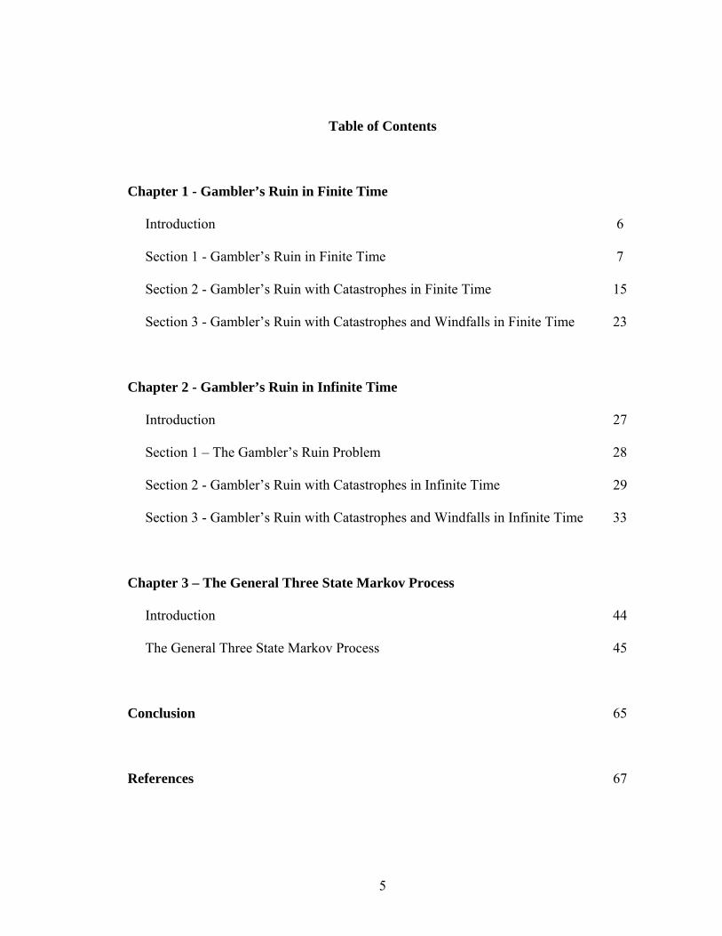
Table of Contents
Chapter 1 - Gambler’s Ruin in Finite Time
Introduction 6
Section 1 - Gambler’s Ruin in Finite Time 7
Section 2 - Gambler’s Ruin with Catastrophes in Finite Time 15
Section 3 - Gambler’s Ruin with Catastrophes and Windfalls in Finite Time 23
Chapter 2 - Gambler’s Ruin in Infinite Time
Introduction 27
Section 1 – The Gambler’s Ruin Problem 28
Section 2 - Gambler’s Ruin with Catastrophes in Infinite Time 29
Section 3 - Gambler’s Ruin with Catastrophes and Windfalls in Infinite Time 33
Chapter 3 – The General Three State Markov Process
Introduction 44
The General Three State Markov Process 45
Conclusion 65
References 67
5
Chapter 1
Gambler’s Ruin in Finite Time
Introduction
In this chapter, the gambler’s ruin probabilities, in finite time, are determined in two
different settings. The gambler’s ruin with catastrophes is solved in Section 2 and then
the gambler’s ruin problem with catastrophes and windfalls is determined in Section 3.
We begin with a key lattice path counting result for solving the classic gambler’s ruin in
finite time. This combinatoric method is extended to solve the gambler’s ruin with
catastrophes and the gambler’s ruin with catastrophes and windfalls, by isolating the
classic gambler’s ruin within these generalized models. There are two path counting
approaches to find the gambler’s ruin with catastrophes in finite time. The first method
avoids catastrophes and produces a solution that is dependent upon the catastrophe
probability only implicitly. The second approach is more direct and is explicitly
catastrophe dependent. The second technique is then used to solve the gambler’s ruin
with catastrophes and windfalls in Section 3.
6
Section 1-1
Gambler’s Ruin in Finite Time
The gambler’s ruin problem is over three hundred fifty years old. It can be traced back to
conversation letters back and forth between Blaise Pascal and Pierre Fermat, see [1].
Pascal considered the problem so difficult that he doubted whether Fermat would be able
to solve it. In Pascal’s opinion, see [1], it was more difficult than all the other probability
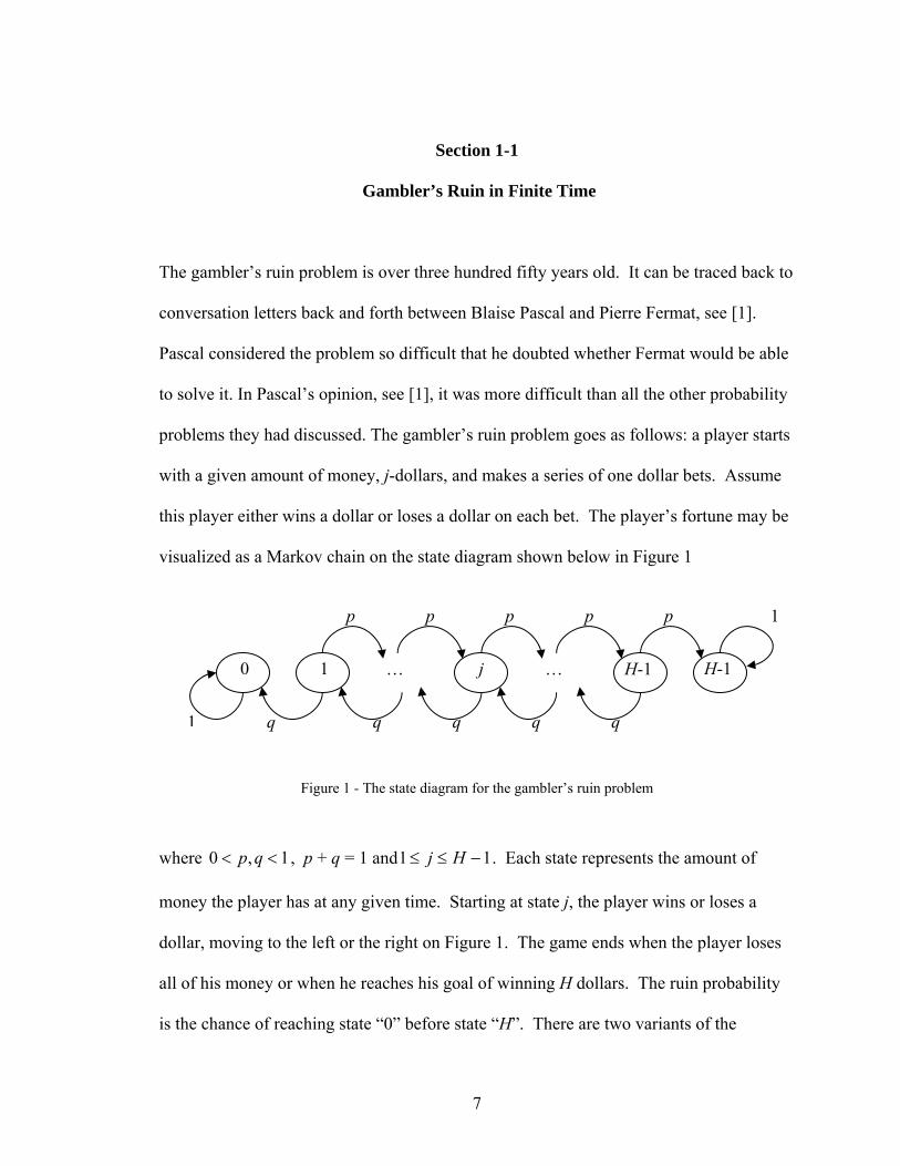
problems they had discussed. The gambler’s ruin problem goes as follows: a player starts
with a given amount of money, j-dollars, and makes a series of one dollar bets. Assume
this player either wins a dollar or loses a dollar on each bet. The player’s fortune may be
visualized as a Markov chain on the state diagram shown below in Figure 1
j 0 1 … … H-1 H-1
q q q q q
p p p p p 1
1
Figure 1 - The state diagram for the gambler’s ruin problem
where , p + q = 1 and1,0 << qp 11 −≤≤ Hj . Each state represents the amount of
money the player has at any given time. Starting at state j, the player wins or loses a
dollar, moving to the left or the right on Figure 1. The game ends when the player loses
all of his money or when he reaches his goal of winning H dollars. The ruin probability
is the chance of reaching state “0” before state “H”. There are two variants of the
7
gambler’s ruin problem: one assumes finite time (or a limited number of bets) and the
other assumes an infinite time (or an unlimited number of bets). The solution to both
gambler’s ruin problems dates back at least to the late 1600’s [1,11]. In addition to
Pascal and Fermat, solutions were obtained by C. Huygens, J. Bernoulli, A. de Moivre,
P. de Montmort and N. Bernoulli, see [1,11 ]. In this chapter, we analyze the finite time
gambler’s ruin problem using lattice path combinatorics.
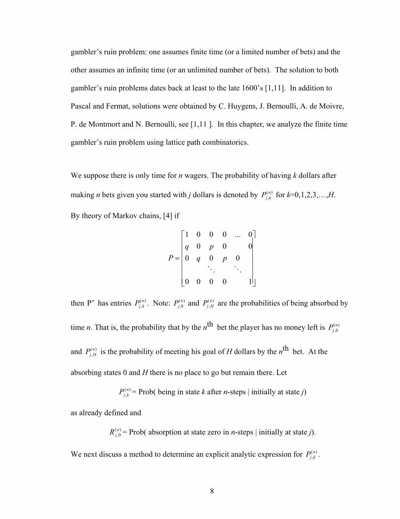
We suppose there is only time for n wagers. The probability of having k dollars after
making n bets given you started with j dollars is denoted by for k=0,1,2,3,…,H. ( ),n
j kP
By theory of Markov chains, [4] if
⎥⎥⎥⎥⎥⎥
⎦
⎤
⎢⎢⎢⎢⎢⎢
⎣
⎡
=
10000
0000000...0001
OO
pqpq
P
then has entries . Note: and are the probabilities of being absorbed by
time n. That is, the probability that by the nth bet the player has no money left is
and is the probability of meeting his goal of H dollars by the nth bet. At the
absorbing states 0 and H there is no place to go but remain there. Let
nΡ ( ),n
j kP ( ),0n
jP ( ),n
j HP
( ),0n
jP
( ),n
j HP
)(,nkjP = Prob( being in state k after n-steps | initially at state j)
as already defined and
)(0,
njR = Prob( absorption at state zero in n-steps | initially at state j).
We next discuss a method to determine an explicit analytic expression for . ( ),n
j kP
8

For simplicity assume 1,1 −≤≤ Hkj . That is, we assume j, k are both inside the box in
Figure 2.
j 0 1 … … H-1 H-1
q q q q q
p p p p p 1
1
Figure 2
Let ( ), ( )n
j kL H represent the collection all lattice paths going from j to k in n-steps, bounded
by horizontal lines y = 0 and y = H and restricted to not hit these boundaries.
H
0
j
k
Figure 3 – Typical Lattice Path
To determine , the problem comes down to finding the number of lattice paths going
from j to k in n-steps not hitting zero or H. The number of lattice paths in
)(,nkjP
( ), ( )n
j kL H is
represented by ( ), ( )n
j kL H .
9

Lemma 1-1.1 For 1,1 −≤≤ Hkj
∑+
=++⎥⎥
⎦
⎤
⎢⎢
⎣
⎡
⎟⎟
⎠
⎞
⎜⎜
⎝
⎛+++
−++−⎟⎟
⎠
⎞
⎜⎜
⎝
⎛+−
+−=1
1
)(, 1)1(
22)1(
2)(
H
l
nkj Hljkn
nHljkn
nHL
where the subscript of “+” means
⎪⎪⎪
⎩
⎪⎪⎪
⎨
⎧
<>
≤≤⎟⎟⎠
⎞⎜⎜⎝
⎛
=⎟⎟⎠
⎞⎜⎜⎝
⎛
+ 0 0
0
xornxif
nxifxn
xn
This result is derived using combinatorics, the reflection principle, and the method of
inclusion/exclusion. The proof may be found in [9, 10].
Rewriting the sum of binomial coefficients in the preceding lemma as nth powers we
obtain a result discovered by Cal Poly Pomona Professor Daniel Marcus, see [7].
Afterwards, it was found out that this result goes back many years, cf. [11].
Lemma 1-1.2 For 10 −≤≤ ma where a, m are whole numbers
∑∑=
−
≡ +
+=⎟⎟⎠
⎞⎜⎜⎝
⎛ m
u
nuua
magww
mgn
1mod)1(1
and where 2exp iwmπ⎧ ⎫= ⎨ ⎬
⎩ ⎭, an root of unity. thm
Combining Lemmas 1-1.1 and 1-1.2 and simplifying gives the following important
proposition.
10
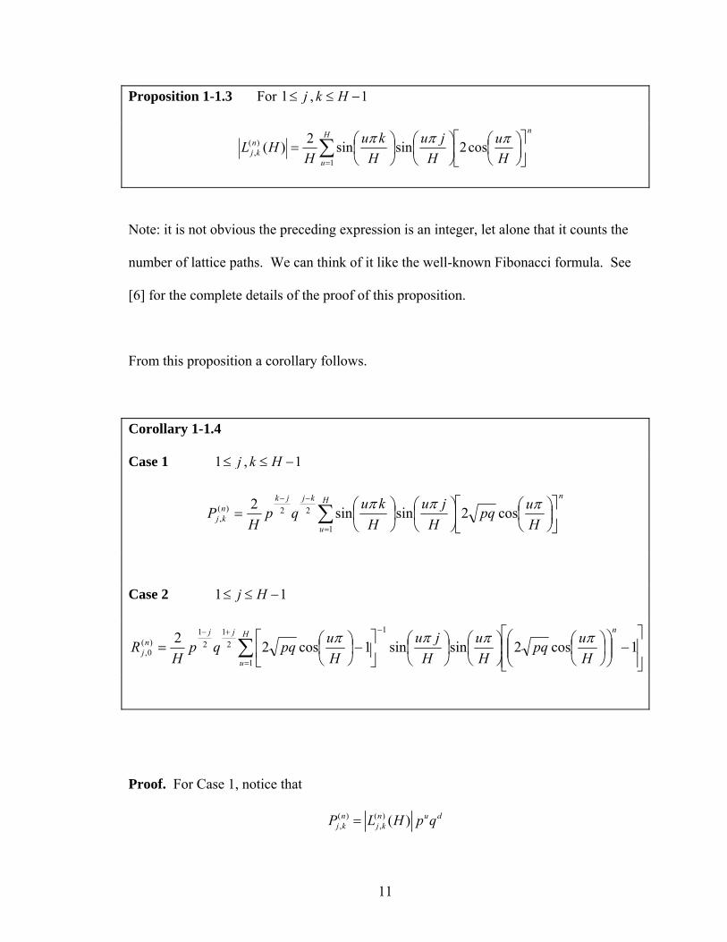
Proposition 1-1.3 For 1 ,j≤ 1k H≤ −
nH
u
nkj H
uH
juH
kuH
HL ⎥⎦
⎤⎢⎣
⎡⎟⎠⎞
⎜⎝⎛
⎟⎠⎞
⎜⎝⎛
⎟⎠⎞
⎜⎝⎛= ∑
=
πππ cos2sinsin2)(1
)(,
Note: it is not obvious the preceding expression is an integer, let alone that it counts the
number of lattice paths. We can think of it like the well-known Fibonacci formula. See
[6] for the complete details of the proof of this proposition.
From this proposition a corollary follows.
Corollary 1-1.4
Case 1 1 j≤ , 1k H≤ −
nH
u
kjjknkj H
upqH
juH
kuqpH
P ⎥⎦
⎤⎢⎣
⎡⎟⎠⎞
⎜⎝⎛
⎟⎠⎞
⎜⎝⎛
⎟⎠⎞
⎜⎝⎛= ∑
=
−− πππ cos2sinsin21
22)(,
Case 2 1 1j H≤ ≤ −
⎥⎥⎦
⎤
⎢⎢⎣
⎡−⎟⎟
⎠
⎞⎜⎜⎝
⎛⎟⎠⎞
⎜⎝⎛
⎟⎠⎞
⎜⎝⎛
⎟⎠⎞
⎜⎝⎛
⎥⎦
⎤⎢⎣
⎡−⎟
⎠⎞
⎜⎝⎛= ∑
=
−+−
1cos2sinsin1cos221
1
21
21
)(0,
nH
u
jjn
j Hupq
Hu
Hju
Hupqqp
HR ππππ
Proof. For Case 1, notice that
( ) ( ), , ( )n n u
j k j kP L H p= dq
11
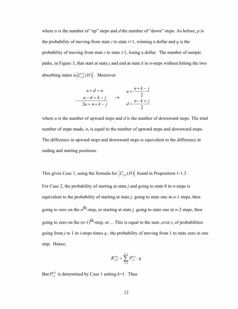
where u is the number of “up” steps and d the number of “down” steps. As before, p is
the probability of moving from state i to state i+1, winning a dollar and q is the
probability of moving from state i to state i-1, losing a dollar. The number of sample
paths, in Figure 3, that start at state j and end at state k in n-steps without hitting the two
absorbing states is )()(, HL nkj . Moreover
2
22
n k ju d n uu d k j
n k jdu n k j
+ −+ = =→− = −
− +== + −
where u is the number of upward steps and d is the number of downward steps. The total
number of steps made, n, is equal to the number of upward steps and downward steps.
The difference in upward steps and downward steps is equivalent to the difference in
ending and starting positions.
This gives Case 1, using the formula for )(, HLnkj found in Proposition 1-1.3 .
For Case 2, the probability of starting at state j and going to state 0 in n-steps is
equivalent to the probability of starting at state j, going to state one in n-1 steps, then
going to zero on the nth-step, or starting at state j, going to state one in n-2 steps, then
going to zero on the (n-1)th-step, or… This is equal to the sum ,over i, of probabilities
going from j to 1 in i-steps times q , the probability of moving from 1 to state zero in one
step. Hence,
qPRn
i
ij
nj ⋅= ∑
−
=
1
1
)(1,
)(0,
But is determined by Case 1 setting k=1. Thus )(1,i
jP
12
qHupq
Hju
Huqp
HR
iH
u
jn
i
jn
j ⋅⎥⎦
⎤⎢⎣
⎡⎟⎠⎞
⎜⎝⎛
⎟⎠⎞
⎜⎝⎛
⎟⎠⎞
⎜⎝⎛= ∑∑
=
−−
=
− πππ cos2sinsin21
211
1
21
)(0,
iH
u
n
i
jj
Hupq
Hju
Huqqp
H ⎥⎦
⎤⎢⎣
⎡⎟⎠⎞
⎜⎝⎛
⎟⎠⎞
⎜⎝⎛
⎟⎠⎞
⎜⎝⎛= ∑∑
=
−
=
−− πππ cos2sinsin21
1
1
21
21
∑ ∑=
−
=
+−
⎥⎦
⎤⎢⎣
⎡⎟⎠⎞
⎜⎝⎛
⎟⎠⎞
⎜⎝⎛
⎟⎠⎞
⎜⎝⎛=
H
u
n
i
ijj
Hupq
Hju
Huqp
H 1
1
1
21
21
cos2sinsin2 πππ
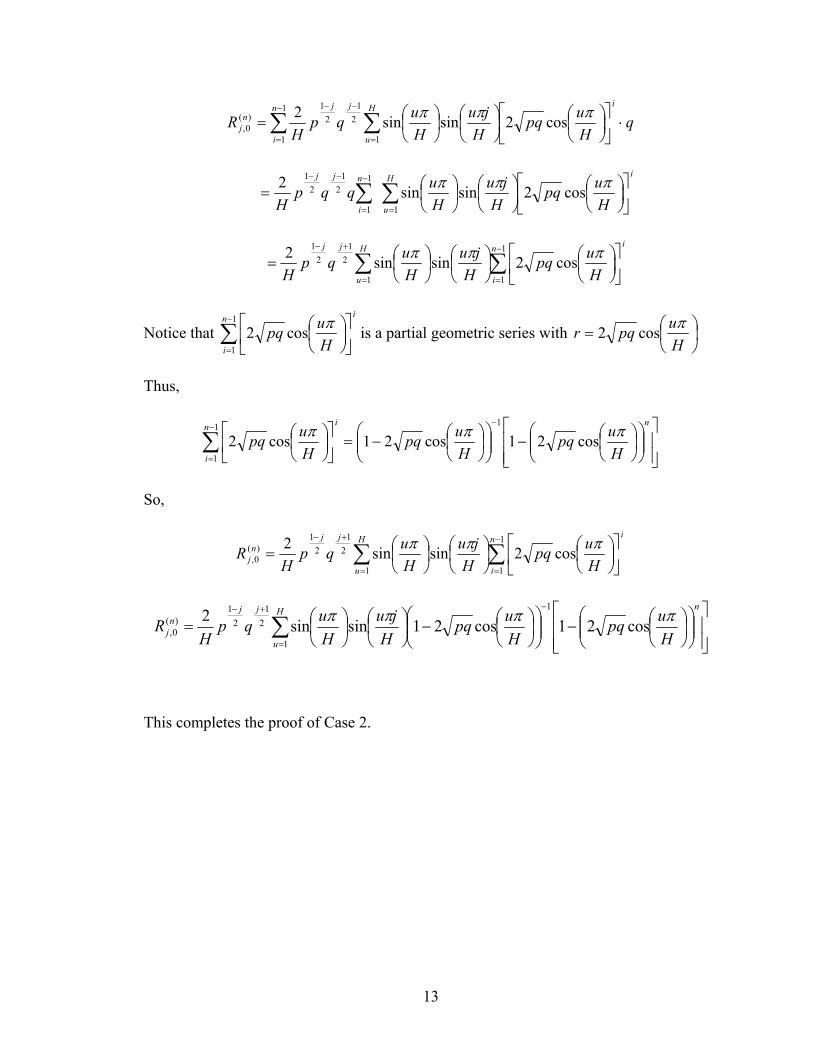
Notice that ∑−
=⎥⎦
⎤⎢⎣
⎡⎟⎠⎞
⎜⎝⎛1
1cos2
n
i
i
Hupq π is a partial geometric series with ⎟
⎠⎞
⎜⎝⎛=
Hupqr πcos2
Thus,
⎥⎥⎦
⎤
⎢⎢⎣
⎡⎟⎟⎠
⎞⎜⎜⎝
⎛⎟⎠⎞
⎜⎝⎛−⎟⎟
⎠
⎞⎜⎜⎝
⎛⎟⎠⎞
⎜⎝⎛−=⎥
⎦
⎤⎢⎣
⎡⎟⎠⎞
⎜⎝⎛
−−
=∑
nn
i
i
Hupq
Hupq
Hupq πππ cos21cos21cos2
11
1
So,
∑ ∑=
−
=
+−
⎥⎦
⎤⎢⎣
⎡⎟⎠⎞
⎜⎝⎛
⎟⎠⎞
⎜⎝⎛
⎟⎠⎞
⎜⎝⎛=
H
u
n
i
ijjn
j Hupq
Hju
Huqp
HR
1
1
1
21
21
)(0, cos2sinsin2 πππ
∑=
−+−
⎥⎥⎦
⎤
⎢⎢⎣
⎡⎟⎟⎠
⎞⎜⎜⎝
⎛⎟⎠⎞
⎜⎝⎛−⎟⎟
⎠
⎞⎜⎜⎝
⎛⎟⎠⎞
⎜⎝⎛−⎟
⎠⎞
⎜⎝⎛
⎟⎠⎞
⎜⎝⎛=
H
u
njjn
j Hupq
Hupq
Hju
Huqp
HR
1
1
21
21
)(0, cos21cos21sinsin2 ππππ
This completes the proof of Case 2.
13

Roulette Example
A roulette player starts with a given amount of money, j= 1,2,3 or 4 dollars, and makes a
series of one dollar bets. Assume the player either wins a dollar or loses a dollar on each
bet of red or black.
0 1 … 5
18/38 18/38 18/38
1 120/38 20/38 20/38 20/38
18/38
j …
Figure 4
H= 5 (maximum value), p=18/38 (probability of a win, placing a bet on black or red),
q=20/38 (probability of a loss), j= starting amount
)(,nkjP have been calculated in the following table listed as P(j,k).
j P(j,0) P(j,1) P(j,2) P(j,3) P(j,4) P(j,5) n = 5
1.0000 0.7230 0.0000 0.1472 0.0000 0.0795 0.0503 2.0000 0.4151 0.1636 0.0000 0.2355 0.0000 0.1858 3.0000 0.2548 0.0000 0.2617 0.0000 0.1472 0.3363 4.0000 0.0767 0.1090 0.0000 0.1636 0.0000 0.6507 n = 10 1.0000 0.7902 0.0327 0.0000 0.0477 0.0000 0.1294 2.0000 0.5934 0.0000 0.0857 0.0000 0.0477 0.2732 3.0000 0.3748 0.0589 0.0000 0.0857 0.0000 0.4807 4.0000 0.1972 0.0000 0.0589 0.0000 0.0327 0.7111 n = 50 1.0000 0.8398 0.0000 0.0000 0.0000 0.0000 0.1602 2.0000 0.6618 0.0000 0.0000 0.0000 0.0000 0.3382 3.0000 0.4640 0.0000 0.0000 0.0000 0.0000 0.5360 4.0000 0.2442 0.0000 0.0000 0.0000 0.0000 0.7558 n = 500 1.0000 0.8398 0.0000 0.0000 0.0000 0.0000 0.1602 2.0000 0.6618 0.0000 0.0000 0.0000 0.0000 0.3382 3.0000 0.4640 0.0000 0.0000 0.0000 0.0000 0.5360 4.0000 0.2442 0.0000 0.0000 0.0000 0.0000 0.7558
14

Section 1-2
Gambler’s Ruin with Catastrophes in Finite Time
In this section, a generalization of the original gambler’s ruin problem is considered.
An added probability, r, of a catastrophe is assumed. That is, a chance that at any point
during the betting a player can lose all of his money is now possible. A computer system
may be modeled in a similar manner. A hard drive may be thought of as adding bytes of
information with probability p and losing or processing information with probability q,
but at any point in time the hard drive might crash losing all of its information. The
lattice path counting result found in Proposition 1-1.3, some algebra, and basic concepts
of probability, provide the tools required to solve the gambler’s ruin problem with
catastrophes. In this section, we present two different methods of solution. The second
method appears more general, allowing us to consider more general related problems (see
Section 3). However, in this present section, our primary goal is to obtain a general
analytic expression for the probability of being ruined (in finite time) when the gambler’s
ruin problem is augmented to include catastrophe probabilities.
Motivated by queueing and population models, consider that at any step k=1,2,..(H-1)
there is a probability r of a catastrophe taking you to state zero as shown in Figure 5.
15

0 1 2 j … … H-1 H
q+r q q q q q
p p p p p p
1
1
r
Figure 5 - Gambler’s Ruin with Catastrophes
where 1p q r+ + = , 1,,0 <≤ rqp , and 11 −≤≤ Hj . With transition matrix
⎥⎥⎥⎥⎥⎥⎥⎥⎥
⎦
⎤
⎢⎢⎢⎢⎢⎢⎢⎢⎢
⎣
⎡+
=
1000
000
00000000...00001
pqr
pqrpqr
prq
POOOM
MO
then has entries . nΡ ( ),n
j kP
Note: and are the probabilities of being absorbed by time n. As before, we wish
to find an explicit representation for
( ),0n
jP ( ),n
j HP
( ),n
j kP . Assume 1,1 −≤≤ Hkj as shown in Figure 6.
Again, let
)(,nkjP = Prob( being in state k in n-steps | initially at state j).
)(0,
njR = Prob( absorption at state zero in n-steps | initially at state j).
16
0 1 2 j … … H-1 H
q+r q q q q q
p p p p p p
r
1
1
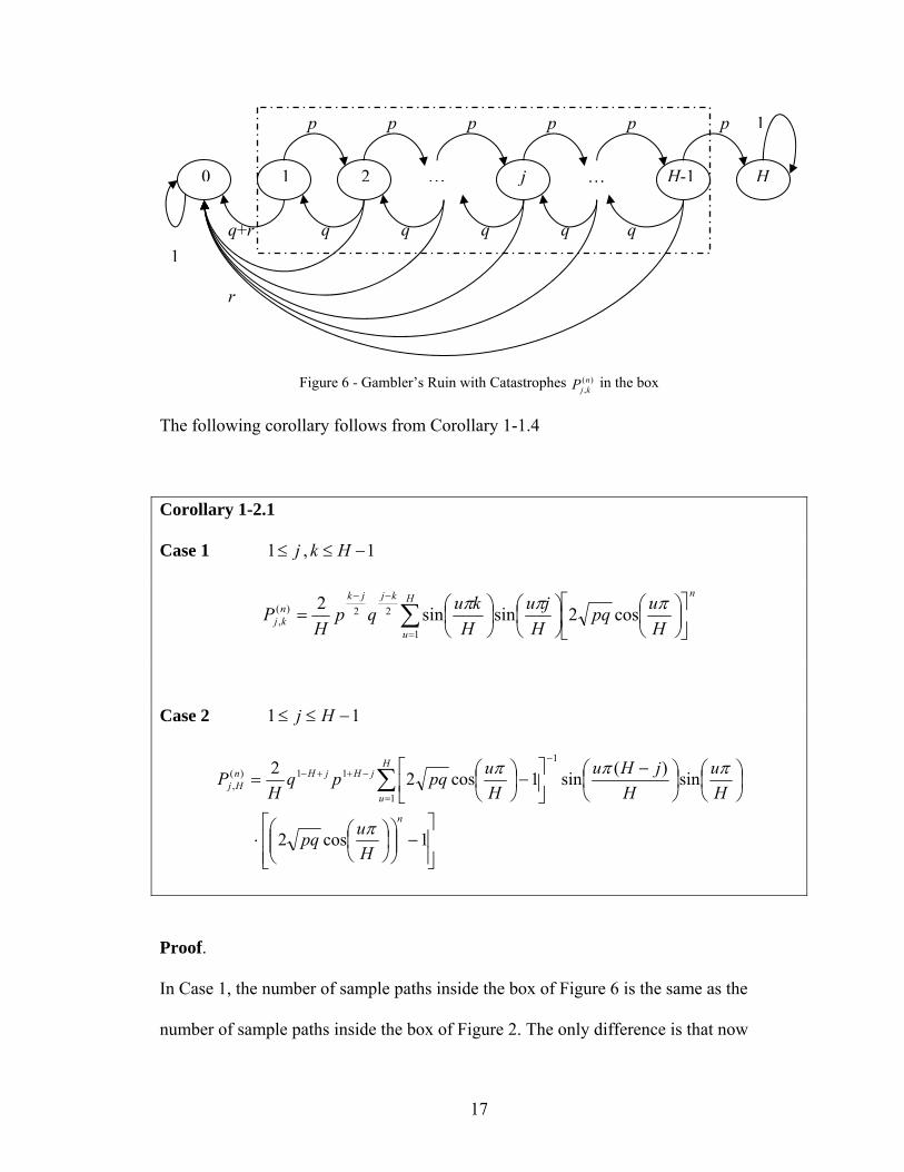
Figure 6 - Gambler’s Ruin with Catastrophes P in the box )(,nkj
The following corollary follows from Corollary 1-1.4
Corollary 1-2.1
Case 1 , 1 j≤ 1k H≤ −
nH
u
kjjknkj H
upqH
juH
kuqpH
P ⎥⎦
⎤⎢⎣
⎡⎟⎠⎞
⎜⎝⎛
⎟⎠⎞
⎜⎝⎛
⎟⎠⎞
⎜⎝⎛= ∑
=
−− πππ cos2sinsin21
22)(,
Case 2 11 −≤≤ Hj
⎥⎥⎦
⎤
⎢⎢⎣
⎡−⎟⎟
⎠
⎞⎜⎜⎝
⎛⎟⎠⎞
⎜⎝⎛⋅
⎟⎠⎞
⎜⎝⎛
⎟⎠⎞
⎜⎝⎛ −
⎥⎦
⎤⎢⎣
⎡−⎟
⎠⎞
⎜⎝⎛= ∑
=
−−++−
1cos2
sin)(sin1cos221
111)(
,
n
H
u
jHjHnHj
Hupq
Hu
HjHu
Hupqpq
HP
π
πππ
Proof.
In Case 1, the number of sample paths inside the box of Figure 6 is the same as the
number of sample paths inside the box of Figure 2. The only difference is that now
17
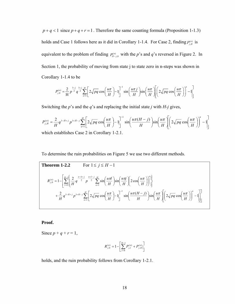
1<+ qp since 1p q r+ + = . Therefore the same counting formula (Proposition 1-1.3)
holds and Case 1 follows here as it did in Corollary 1-1.4. For Case 2, finding ( ),n
j HP is
equivalent to the problem of finding ( ),0
nH jP −
with the p’s and q’s reversed in Figure 2. In
Section 1, the probability of moving from state j to state zero in n-steps was shown in
Corollary 1-1.4 to be
11 1( ) 2 2,0
12 cos 1 sin sin 2 cos 1
nj j Hn
ju
u u j u uP p q pq pqH H H Hπ π π π
−− +
=
⎡ ⎤2 ⎡ ⎤ ⎛ ⎞⎛ ⎞ ⎛ ⎞ ⎛ ⎞ ⎛ ⎞= − −⎢ ⎥⎜ ⎟ ⎜ ⎟ ⎜ ⎟ ⎜ ⎟⎜ ⎟⎢ ⎥Η ⎝ ⎠ ⎝ ⎠ ⎝ ⎠ ⎝ ⎠⎣ ⎦ ⎝ ⎠⎢ ⎥⎣ ⎦∑
Switching the p’s and the q’s and replacing the initial state j with H-j gives,
⎥⎥⎦
⎤
⎢⎢⎣
⎡−⎟⎟
⎠
⎞⎜⎜⎝
⎛⎟⎠⎞
⎜⎝⎛
⎟⎠⎞
⎜⎝⎛
⎟⎠⎞
⎜⎝⎛ −
⎥⎦
⎤⎢⎣
⎡−⎟
⎠⎞
⎜⎝⎛= ∑
=
−−++− 1cos2sin)(sin1cos22
1
111)(
,
nH
u
jHjHnHj H
upqHu
HjHu
Hupqpq
HP ππππ
which establishes Case 2 in Corollary 1-2.1.
To determine the ruin probabilities on Figure 5 we use two different methods.
Theorem 1-2.2 For 11 −≤≤ Hj
⎥⎥⎦
⎤
⎥⎥⎦
⎤
⎢⎢⎣
⎡−⎟⎟
⎠
⎞⎜⎜⎝
⎛⎟⎠⎞
⎜⎝⎛
⎟⎠⎞
⎜⎝⎛
⎟⎠⎞
⎜⎝⎛ −
⎥⎦
⎤⎢⎣
⎡−⎟
⎠⎞
⎜⎝⎛+
⎢⎢⎣
⎡
⎪⎭
⎪⎬⎫
⎪⎩
⎪⎨⎧
⎟⎟⎠
⎞⎜⎜⎝
⎛⎟⎠⎞
⎜⎝⎛
⎟⎠⎞
⎜⎝⎛
⎟⎠⎞
⎜⎝⎛−=
∑
∑ ∑
=
−−++−
−
= =
−++−
1cos2sin)(
sin1cos22
cos2sinsin21
1
111
1
0 1
22)(0,
nH
u
jHjH
H
l
nH
u
jlnjknn
j
Hupq
Hu
HjHu
Hupqpq
H
Hu
Hju
Hlupq
HR
ππππ
πππ
Proof.
Since p + q + r = 1,
⎥⎦
⎤⎢⎣
⎡+−= ∑
−
=
)(,
1
0
)(,
)(0, 1 n
Hj
H
l
nlj
nj PPR
holds, and the ruin probability follows from Corollary 1-2.1.
18
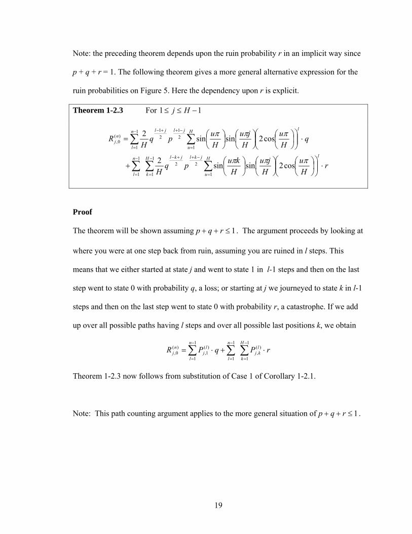
Note: the preceding theorem depends upon the ruin probability r in an implicit way since
p + q + r = 1. The following theorem gives a more general alternative expression for the
ruin probabilities on Figure 5. Here the dependency upon r is explicit.
Theorem 1-2.3 For 11 −≤≤ Hj
∑ ∑∑
∑ ∑−
= =
−++−−
=
−
= =
−++−
⋅⎟⎟⎠
⎞⎜⎜⎝
⎛⎟⎠⎞
⎜⎝⎛
⎟⎠⎞
⎜⎝⎛
⎟⎠⎞
⎜⎝⎛+
⋅⎟⎟⎠
⎞⎜⎜⎝
⎛⎟⎠⎞
⎜⎝⎛
⎟⎠⎞
⎜⎝⎛
⎟⎠⎞
⎜⎝⎛=
1
1 1
221
1
1
1 1
21
21
)(0,
cos2sinsin2
cos2sinsin2
H
k
lH
u
jkljkln
l
n
l
lH
u
jljln
j
rHu
Hju
Hkupq
H
qHu
Hju
Hupq
HR
πππ
πππ
Proof
The theorem will be shown assuming 1≤++ rqp . The argument proceeds by looking at
where you were at one step back from ruin, assuming you are ruined in l steps. This
means that we either started at state j and went to state 1 in l-1 steps and then on the last
step went to state 0 with probability q, a loss; or starting at j we journeyed to state k in l-1
steps and then on the last step went to state 0 with probability r, a catastrophe. If we add
up over all possible paths having l steps and over all possible last positions k, we obtain
∑∑ ∑−
=
−
=
−
=
⋅+⋅=1
1
)(,
1
1
1
1
)(1,
)(0,
H
k
lkj
n
l
n
l
lj
nj rPqPR
Theorem 1-2.3 now follows from substitution of Case 1 of Corollary 1-2.1.
Note: This path counting argument applies to the more general situation of 1≤++ rqp .
19
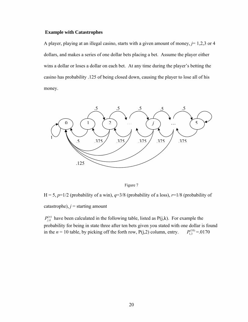
Example with Catastrophes
A player, playing at an illegal casino, starts with a given amount of money, j= 1,2,3 or 4
dollars, and makes a series of one dollar bets placing a bet. Assume the player either
wins a dollar or loses a dollar on each bet. At any time during the player’s betting the
casino has probability .125 of being closed down, causing the player to lose all of his
money.
0 1 2 j … … 5
.5
.5 .5 .5
1
.125
.5
.375.375.375 .375 .375
.5
Figure 7
H = 5, p=1/2 (probability of a win), q=3/8 (probability of a loss), r=1/8 (probability of
catastrophe), j = starting amount
)(,nkjP have been calculated in the following table, listed as P(j,k). For example the
probability for being in state three after ten bets given you stated with one dollar is found in the n = 10 table, by picking off the forth row, P(j,2) column, entry. =.0170 )10(
3,1P
20
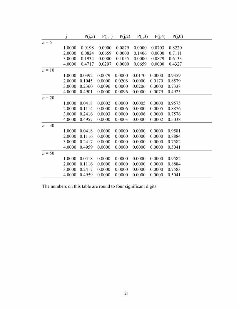
j P(j,5) P(j,1) P(j,2) P(j,3) P(j,4) P(j,0) n = 5 1.0000 0.0198 0.0000 0.0879 0.0000 0.0703 0.8220 2.0000 0.0824 0.0659 0.0000 0.1406 0.0000 0.7111 3.0000 0.1934 0.0000 0.1055 0.0000 0.0879 0.6133 4.0000 0.4717 0.0297 0.0000 0.0659 0.0000 0.4327 n = 10 1.0000 0.0392 0.0079 0.0000 0.0170 0.0000 0.9359 2.0000 0.1045 0.0000 0.0206 0.0000 0.0170 0.8579 3.0000 0.2360 0.0096 0.0000 0.0206 0.0000 0.7338 4.0000 0.4901 0.0000 0.0096 0.0000 0.0079 0.4925 n = 20 1.0000 0.0418 0.0002 0.0000 0.0005 0.0000 0.9575 2.0000 0.1114 0.0000 0.0006 0.0000 0.0005 0.8876 3.0000 0.2416 0.0003 0.0000 0.0006 0.0000 0.7576 4.0000 0.4957 0.0000 0.0003 0.0000 0.0002 0.5038 n = 30 1.0000 0.0418 0.0000 0.0000 0.0000 0.0000 0.9581 2.0000 0.1116 0.0000 0.0000 0.0000 0.0000 0.8884 3.0000 0.2417 0.0000 0.0000 0.0000 0.0000 0.7582 4.0000 0.4959 0.0000 0.0000 0.0000 0.0000 0.5041 n = 50 1.0000 0.0418 0.0000 0.0000 0.0000 0.0000 0.9582 2.0000 0.1116 0.0000 0.0000 0.0000 0.0000 0.8884 3.0000 0.2417 0.0000 0.0000 0.0000 0.0000 0.7583 4.0000 0.4959 0.0000 0.0000 0.0000 0.0000 0.5041 The numbers on this table are round to four significant digits.
21
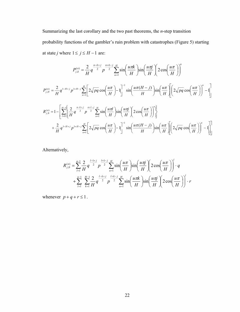
Summarizing the last corollary and the two past theorems, the n-step transition
probability functions of the gambler’s ruin problem with catastrophes (Figure 5) starting
at state j where are: 11 −≤≤ Hj
nH
u
jknjknnkj H
uH
juH
kupqH
P ⎟⎟⎠
⎞⎜⎜⎝
⎛⎟⎠⎞
⎜⎝⎛
⎟⎠⎞
⎜⎝⎛
⎟⎠⎞
⎜⎝⎛= ∑
=
−++− πππ cos2sinsin21
22)(,
⎥⎥⎦
⎤
⎢⎢⎣
⎡−⎟⎟
⎠
⎞⎜⎜⎝
⎛⎟⎠⎞
⎜⎝⎛
⎟⎠⎞
⎜⎝⎛
⎟⎠⎞
⎜⎝⎛ −
⎥⎦
⎤⎢⎣
⎡−⎟
⎠⎞
⎜⎝⎛= ∑
=
−−++− 1cos2sin)(sin1cos22
1
111)(
,
nH
u
jHjHnHj H
upqHu
HjHu
Hupqpq
HP ππππ
⎥⎥⎦
⎤
⎥⎥⎦
⎤
⎢⎢⎣
⎡−⎟⎟
⎠
⎞⎜⎜⎝
⎛⎟⎠⎞
⎜⎝⎛
⎟⎠⎞
⎜⎝⎛
⎟⎠⎞
⎜⎝⎛ −
⎥⎦
⎤⎢⎣
⎡−⎟
⎠⎞
⎜⎝⎛+
⎢⎢⎣
⎡
⎪⎭
⎪⎬⎫
⎪⎩
⎪⎨⎧
⎟⎟⎠
⎞⎜⎜⎝
⎛⎟⎠⎞
⎜⎝⎛
⎟⎠⎞
⎜⎝⎛
⎟⎠⎞
⎜⎝⎛−=
∑
∑ ∑
=
−−++−
−
= =
−++−
1cos2sin)(sin1cos22
cos2sinsin21
1
111
1
0 1
22)(0,
nH
u
jHjH
H
l
nH
u
jlnjknn
j
Hupq
Hu
HjHu
Hupqpq
H
Hu
Hju
Hlupq
HR
ππππ
πππ
Alternatively,
∑ ∑∑
∑ ∑−
= =
−++−−
=
−
= =
−++−
⋅⎟⎟⎠
⎞⎜⎜⎝
⎛⎟⎠⎞
⎜⎝⎛
⎟⎠⎞
⎜⎝⎛
⎟⎠⎞
⎜⎝⎛+
⋅⎟⎟⎠
⎞⎜⎜⎝
⎛⎟⎠⎞
⎜⎝⎛
⎟⎠⎞
⎜⎝⎛
⎟⎠⎞
⎜⎝⎛=
1
1 1
221
1
1
1 1
21
21
)(0,
cos2sinsin2
cos2sinsin2
H
k
lH
u
jkljkln
l
n
l
lH
u
jljln
j
rHu
Hju
Hkupq
H
qHu
Hju
Hupq
HR
πππ
πππ
whenever . 1≤++ rqp
22
Section 1-3
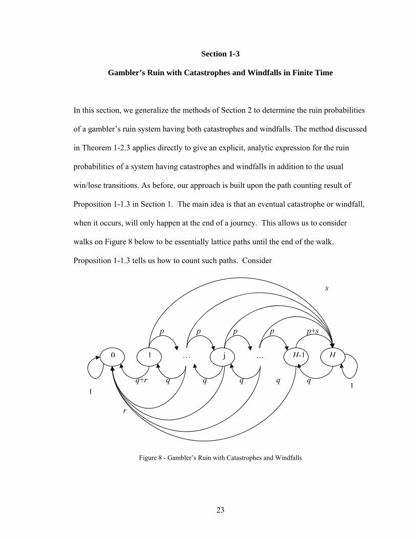
Gambler’s Ruin with Catastrophes and Windfalls in Finite Time
In this section, we generalize the methods of Section 2 to determine the ruin probabilities
of a gambler’s ruin system having both catastrophes and windfalls. The method discussed
in Theorem 1-2.3 applies directly to give an explicit, analytic expression for the ruin
probabilities of a system having catastrophes and windfalls in addition to the usual
win/lose transitions. As before, our approach is built upon the path counting result of
Proposition 1-1.3 in Section 1. The main idea is that an eventual catastrophe or windfall,
when it occurs, will only happen at the end of a journey. This allows us to consider
walks on Figure 8 below to be essentially lattice paths until the end of the walk.
Proposition 1-1.3 tells us how to count such paths. Consider
Figure 8 - Gambler’s Ruin with Catastrophes and Windfalls
q+r
0 1 j … … HH-1
q q q q q
p p p p p+s
11
r
s
23
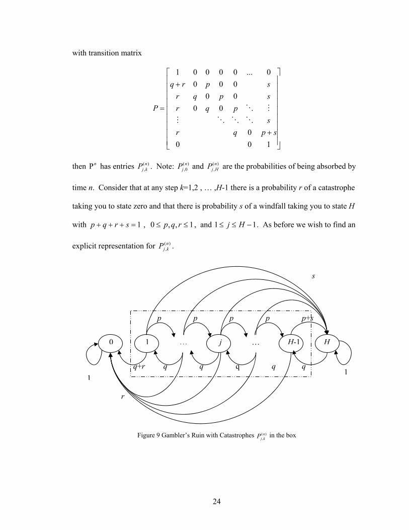
with transition matrix
⎥⎥⎥⎥⎥⎥⎥⎥⎥
⎦
⎤
⎢⎢⎢⎢⎢⎢⎢⎢⎢
⎣
⎡
+
+
=
1000
0000000
0...00001
spqrs
pqrspqrsprq
POOOM
MO
then has entries . Note: and are the probabilities of being absorbed by
time n. Consider that at any step k=1,2 , … ,H-1 there is a probability r of a catastrophe
taking you to state zero and that there is probability s of a windfall taking you to state H
with ,
nΡ ( ),n
j kP ( ),0n
jP ( ),n
j HP
1=+++ srqp 1,,0 ≤≤ rqp , and 11 −≤≤ Hj . As before we wish to find an
explicit representation for . )(,nkjP
q+r
0 1 j … … HH-1
q q q q q
p p p p p+s
11
r
s
Figure 9 Gambler’s Ruin with Catastrophes P in the box )(,nkj
24

The transition probability functions are determined for two distinct cases by the following
corollary.
Corollary 1-3.1
Case 1 For 1,1 −≤≤ Hkj
nH
u
kjjknkj H
upqH
juH
kuqpH
P ⎥⎦
⎤⎢⎣
⎡⎟⎠⎞
⎜⎝⎛
⎟⎠⎞
⎜⎝⎛
⎟⎠⎞
⎜⎝⎛= ∑
=
−− πππ cos2sinsin21
22)(,
Case 2 For 11 −≤≤ Hj
∑ ∑∑
∑ ∑−
= =
−++−−
=
−
= =
−++−
⋅⎟⎟⎠
⎞⎜⎜⎝
⎛⎟⎠⎞
⎜⎝⎛
⎟⎠⎞
⎜⎝⎛
⎟⎠⎞
⎜⎝⎛+
⋅⎟⎟⎠
⎞⎜⎜⎝
⎛⎟⎠⎞
⎜⎝⎛
⎟⎠⎞
⎜⎝⎛
⎟⎠⎞
⎜⎝⎛=
1
1 1
221
1
1
1 1
21
21
)(0,
cos2sinsin2
cos2sinsin2
H
k
lH
u
jkljkln
l
n
l
lH
u
jljln
j
rHu
Hju
Hkupq
H
qHu
Hju
Hupq
HR
πππ
πππ
Proof.
For Case 1, the proof follows as before from Proposition 1-1.3. Case 2 follows from the
previous path counting result discussed in Theorem 1-2.3.
□
In a similar way, this path counting technique allows a direct approach for finding the
probability of reaching your goal, , in n steps. This time )(,nHjP
∑∑ ∑−
=
−
=
−
=− ⋅+⋅=
1
1
)(,
1
1
1
1
)(1,
)(,
H
k
lkj
n
l
n
l
lHj
nHj sPpPP
which gives
25
∑ ∑∑
∑ ∑−
= =
−++−−
=
−
= =
−+++−
⋅⎟⎟⎠
⎞⎜⎜⎝
⎛⎟⎠⎞
⎜⎝⎛
⎟⎠⎞
⎜⎝⎛
⎟⎠⎞
⎜⎝⎛+
⋅⎟⎟⎠
⎞⎜⎜⎝
⎛⎟⎠⎞
⎜⎝⎛
⎟⎠⎞
⎜⎝⎛
⎟⎠⎞
⎜⎝⎛=
1
1 1
221
1
1
1 1
21
21
)(,
cos2sinsin2
cos2sinsin2
H
k
lH
u
jkljkln
l
n
l
lH
u
jljHlnHj
sHu
Hju
Hkupq
H
pHu
Hju
Hupq
HP
πππ
πππ
.
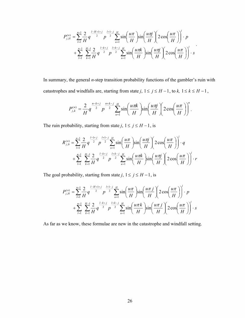
In summary, the general n-step transition probability functions of the gambler’s ruin with
catastrophes and windfalls are, starting from state j, 11 −≤≤ Hj , to k, 11 −≤≤ Hk ,
nH
u
jknjknnkj H
uH
juH
kupqH
P ⎟⎟⎠
⎞⎜⎜⎝
⎛⎟⎠⎞
⎜⎝⎛
⎟⎠⎞
⎜⎝⎛
⎟⎠⎞
⎜⎝⎛= ∑
=
−++− πππ cos2sinsin21
22)(, .
The ruin probability, starting from state j, 11 −≤≤ Hj , is
∑ ∑∑
∑ ∑−
= =
−++−−
=
−
= =
−++−
⋅⎟⎟⎠
⎞⎜⎜⎝
⎛⎟⎠⎞
⎜⎝⎛
⎟⎠⎞
⎜⎝⎛
⎟⎠⎞
⎜⎝⎛+
⋅⎟⎟⎠
⎞⎜⎜⎝
⎛⎟⎠⎞
⎜⎝⎛
⎟⎠⎞
⎜⎝⎛
⎟⎠⎞
⎜⎝⎛=
1
1 1
221
1
1
1 1
21
21
)(0,
cos2sinsin2
cos2sinsin2
H
k
lH
u
jkljkln
l
n
l
lH
u
jljln
j
rHu
Hju
Hkupq
H
qHu
Hju
Hupq
HR
πππ
πππ
The goal probability, starting from state j, 11 −≤≤ Hj , is
∑ ∑∑
∑ ∑−
= =
−++−−
=
−
= =
−+++−
⋅⎟⎟⎠
⎞⎜⎜⎝
⎛⎟⎠⎞
⎜⎝⎛
⎟⎠⎞
⎜⎝⎛
⎟⎠⎞
⎜⎝⎛+
⋅⎟⎟⎠
⎞⎜⎜⎝
⎛⎟⎠⎞
⎜⎝⎛
⎟⎠⎞
⎜⎝⎛
⎟⎠⎞
⎜⎝⎛=
1
1 1
221
1
1
1 1
21
21
)(,
cos2sinsin2
cos2sinsin2
H
k
lH
u
jkljkln
l
n
l
lH
u
jljHlnHj
sHu
Hju
Hkupq
H
pHu
Hju
Hupq
HP
πππ
πππ
As far as we know, these formulae are new in the catastrophe and windfall setting.
26
Chapter 2
Gambler’s Ruin in Infinite Time
Introduction
In this chapter, we again consider the classical gambler’s ruin problem but with an
infinite amount of time. More generally, we reconsider each of the three models
presented in Chapter 1 under the assumption of having an indefinite amount of time until
absorption. This time, our techniques do not explicitly use path counting. The problem
is addressed as solving a system of recurrence relations under appropriate boundary
conditions. Two techniques are employed: difference equations and probability
generating functions. In particular, the infinite time gambler’s ruin with catastrophes
problem is solved in Section 2 using the theory of second order, constant coefficient
recurrence relations and some calculus and probability theory to hold it all together. This
result and the method are then generalized in Section 3 to solve the gambler’s ruin with
both catastrophes and windfalls in infinite time using difference equation techniques. An
interesting probability generating function approach may also be used to determine the
ruin probabilities in the catastrophe and windfall case. This solution method is also
presented in Section 3.
27

Section 2-1
The Gambler’s Ruin Problem
We reconsider the classical gambler’s ruin Problem but now with an infinite amount of
time,
… j 0 1 … H-1 H-1
q q q q q
p p p p p 1
1
Figure 10 - The state diagram for the gambler’s ruin problem
where , p + q = 1 and1,0 << qp 11 −≤≤ Hj . The ruin probability is the chance of
eventually reaching state “0” before state “H”. The classical gambler’s ruin problem in
infinite time has the following elegant solution, see [4, 11].
⎪⎪⎪⎪
⎭
⎪⎪⎪⎪
⎬
⎫
⎪⎪⎪⎪
⎩
⎪⎪⎪⎪
⎨
⎧
=−
≠
⎟⎟⎠
⎞⎜⎜⎝
⎛−
⎟⎟⎠
⎞⎜⎜⎝
⎛−⎟⎟
⎠
⎞⎜⎜⎝
⎛
=<=
qpforHj
qpfor
pq
pq
pq
TTPRH
Hj
Hjj
1
1)( 0
The problem has been solved in many ways ([11]).
28

Section 2-2
Gambler’s Ruin with Catastrophes in Infinite Time
This section looks at the same set-up as in Section 1-2 but with infinite time. We are
looking for the ruin probabilities, that is, probabilities of eventual absorption at state zero.
In this section, we derive expressions for both the ruin probabilities and the probability of
reaching our goal, H, given that you start at state j. These are obtained using the theory
of linear, constant coefficient recurrence relations.
For infinite time, recall this Markov chain was first described in Section 2 of Chapter 1.
0 1 2 j … … H-1 H
q+r q q q q q
p p p p p p
1
1
r
Figure 11 - Gambler’s Ruin with Catastrophes
Let
jR = Prob(eventual absorption at state zero | initially at state j)
and
jP = Prob(eventual absorption at state H | initially at state j).
29
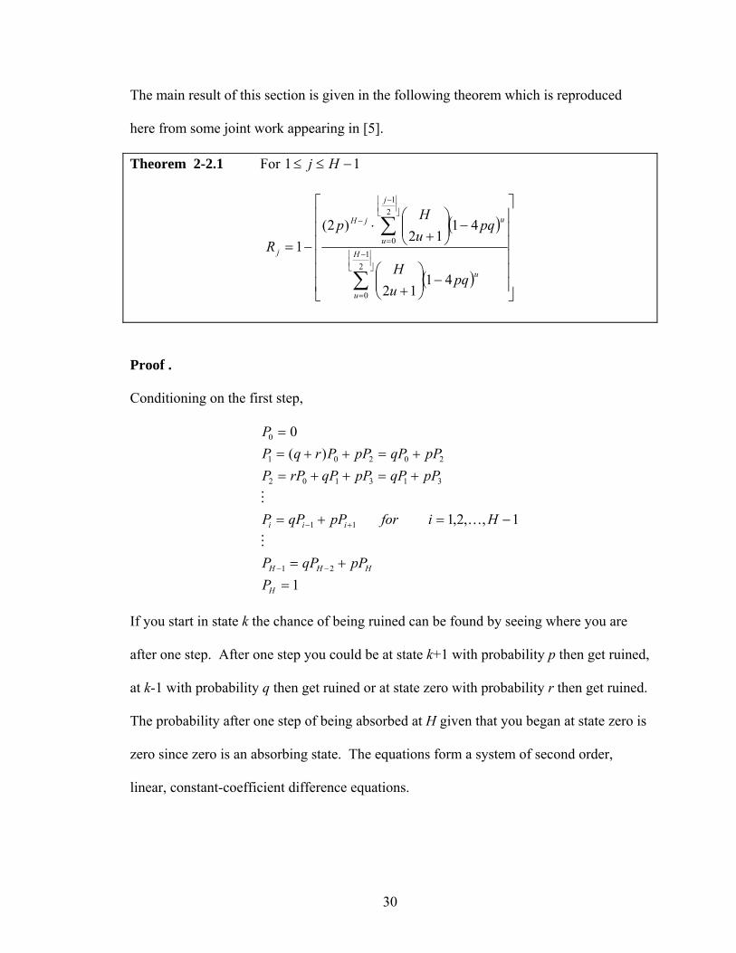
The main result of this section is given in the following theorem which is reproduced
here from some joint work appearing in [5].
Theorem 2-2.1 For 11 −≤≤ Hj
( )
( ) ⎥⎥⎥⎥⎥⎥
⎦
⎤
⎢⎢⎢⎢⎢⎢
⎣
⎡
−⎟⎟⎠
⎞⎜⎜⎝
⎛+
−⎟⎟⎠
⎞⎜⎜⎝
⎛+
⋅−=
∑
∑⎥⎦⎥
⎢⎣⎢ −
=
⎥⎦⎥
⎢⎣⎢ −
=
−
21
0
21
0
4112
4112
)2(1
H
u
u
j
u
ujH
j
pquH
pquH
pR
Proof .
Conditioning on the first step,
1
1,,2,1
)(0
21
11
313102
20201
0
=+=
−=+=
+=++=+=++=
=
−−
+−
H
HHH
iii
PpPqPP
HiforpPqPP
pPqPpPqPrPPpPqPpPPrqP
P
M
K
M
If you start in state k the chance of being ruined can be found by seeing where you are
after one step. After one step you could be at state k+1 with probability p then get ruined,
at k-1 with probability q then get ruined or at state zero with probability r then get ruined.
The probability after one step of being absorbed at H given that you began at state zero is
zero since zero is an absorbing state. The equations form a system of second order,
linear, constant-coefficient difference equations.
30

Thus for ,1,...,3,2,1 −= Hk
011 =+− −+ kkk qPPpP
with characteristic equation,
02 =+− qxpx .
The roots of this equation are p
pq2
411 −±. Note that these roots are distinct since r
is positive. Hence the general solution of the recurrence is of the form (see [8])
kk
k ppq
cp
pqcP
⎥⎥⎦
⎤
⎢⎢⎣
⎡ −−+
⎥⎥⎦
⎤
⎢⎢⎣
⎡ −+=
2411
2411
21
where and are constants to be determined by the two boundary conditions 1c 2c
00 =P and . This gives 1=HP
HH
ppq
cp
pqc
cc
⎥⎥⎦
⎤
⎢⎢⎣
⎡ −−+
⎥⎥⎦
⎤
⎢⎢⎣
⎡ −+=
+=
2411
2411
1
0
21
21
with solution
( ) ( )HH
H
pqpq
pc
cc
411411
)2(1
12
−−−−+=
−=
Thus,
( ) ( ) ⎪⎭
⎪⎬⎫
⎪⎩
⎪⎨⎧
⎥⎥⎦
⎤
⎢⎢⎣
⎡ −−−
⎥⎥⎦
⎤
⎢⎢⎣
⎡ −+⋅
−−−−+=
kk
HH
H
k ppq
ppq
pqpq
pP2
4112
411
411411
)2(
31
( ) ( )( ) ( )HH
kkkH
kpqpq
pqpqpP
411411
411411)2(
−−−−+
⎥⎦⎤
⎢⎣⎡ −−−−+⋅
=
−
=kP( )
( ) ⎥⎥⎥⎥⎥⎥
⎦
⎤
⎢⎢⎢⎢⎢⎢
⎣
⎡
−⎟⎟⎠
⎞⎜⎜⎝
⎛+
−⎟⎟⎠
⎞⎜⎜⎝
⎛+
⋅
∑
∑⎥⎦⎥
⎢⎣⎢ −
=
⎥⎦⎥
⎢⎣⎢ −
=
−
21
0
21
0
4112
4112
)2(
H
u
u
k
u
ukH
pquH
pquH
p
So,
kk PR −= 1 ,
completing the proof.
32
Section 2-3
Gambler’s Ruin with Catastrophes and Windfalls in Infinite Time
In this section, we consider a system of linear constant coefficient recurrence relations for
the ruin probabilities of Figure 12 given that you start at state j. We present two methods
of solution. The first approach uses probability generating functions. Our second
solution method (which we gratefully acknowledge was suggested by thesis committee
member, Dr. Randall J. Swift) is a difference equation approach which essentially
generalizes the arguments presented in the previous section.
Reconsider the Markov chain illustrated in Figure 12.
q+r
0 1 j … … HH-1
q q q q q
p p p p p+s
11
r
s
Figure 12 - Gambler’s Ruin with Catastrophes and Windfalls
33
We seek the probability of eventually being ruined, = Prob(eventual absorption at state
zero | initially at state j).
jR
Theorem 2-3.1 For the Markov chain described by Figure 12, the are given below. jR
Hiforb
Hkforqra
qR
qpa
qpa
baR
ppqppR
R
iii
k
kj
j
kkj
,...,2,1,0
and ,,...,3,2
1
where
1
12
11
11
0
0
22
12
212
22
1
21
222
21
221
1
0
=⎟⎟⎠
⎞⎜⎜⎝
⎛+=
==
−=
=
=
++−−+
=
=
++
−=∑
ρβ
ρα
ρρβρραρρρβραρβρραρ
where
qpq
qpq
2411
2411
21
−−=
−+= ρρ
)(1and
)(1
2112 ρρβ
ρρα
−=
−=
34
Proof.
Conditioning on the first step gives,
0
1,...,2,1
1
21
11
312
201
0
=++=
−=++=
++=++=
=
−−
+−
H
HHH
iii
RrpRqRR
HirpRqRR
rpRqRRrpRqRR
R
M
M
where . So 1=+++ srqp
rpRqRR iii ++= +− 11
for with initial conditions, 1,...,2,1 −= Hi 10 =R and 0=HR .
rqRRpR nnn −=+− −+ 11
The ruin probabilities, ,can be found using the technique of generating functions (see
page 10 of [13]).
iR
Let
∑=
=H
i
ii xRxR
0)( and ∑
−
=
=1
1)(
H
i
irxxD
Beginning with
rqRRpR nnn −=+− −+ 11
and multiplying through by gives, nx
nnn
nn
nn rxxqRxRxpR −=+− −+ 11
35
∑∑∑∑−
=
−
=−
−
=
−
=+ −=+−
1
1
1
11
1
1
1
11
H
n
nH
n
nn
H
n
nn
H
n
nn xrxRqxRxRp
[ ] ∑∑∑ −
=
−−
=
−−
−
=
++
−=+−−1
1
11
1
11
1
1
11
1)(H
n
nH
n
nn
H
n
nn
xrxxRqxxRx
xRp
[ ] [ ] [ ] ( )( )x
xrxxRxRqxxRx
xRxRp HH
H −−−
=−+−−−− −
−− 1
1)(1)(1)( 1
11
1
Multiplying through by , )1( xx −
[ ] [ ] ( )( )12
11
21
1
)()1(1)()1()1(1)(−
−−
−−=
−−+−−−−−−H
HH
xrx
xRxRxqxxRxxxxRxRp
( ) )1(1)1()1)(1( )()1()()1()()1(
11
121
2
xxqRxrxxxxRxpxRxqxxRxxxRxp
HH
H −+−−−++−=
−+−−−+
−−
Solving for , )(xR
[ ]( ) )1(1)1()1)(1(
)1()1()1()(1
112
1
2
xxqRxrxxxxRxpxqxxxxpxR
HH
H −+−−−++−=
−+−−−+
−−
[ ]( ) )1()1()1)(1(1
)1)((1
1112
2
xxqRxxxRxpxrxqxxpxxR
HH
H −+−++−+−−=
+−−+
−−
Dividing through by , )1( x−
( ) 111
122 )1(
)1(1))(( +
−
−
+−++−−−
=+− HH
H
xqRxxRpxxrxqxxpxR
Factoring out a q,
( ) 111
122 )1(
)1(11)( +
−
−
+−++−−−
=⎟⎟⎠
⎞⎜⎜⎝
⎛+− H
H
H
xqRxxRpxxrx
qpx
qxxqR
36

The roots of the quadratic on the left hand side of the preceding equation are,
qpqq
pqqqq
pqq
2411
2
411
2
411
,22
2
21
−±=
−±=
−⎟⎟⎠
⎞⎜⎜⎝
⎛±
=ρρ
1R and may now be found. Note that 1−HR 21 ρρ ≠ assuming r>0 or s>0. We have
( ) 111
12
21 )1()1(
1))()(( +−
−
+−++−−−
=−− HH
H
xqRxxRpxxrxxxxqR ρρ
Recall the formula for the finite sum of a geometric series
221
...11
1 −−
++++=−
− HH
xxxx
x
So,
[ ] 111
22221 )1(...1))()(( +
−− +−++++++−=−− H
HH xqRxxRpxxxrxxxxqR ρρ
Dividing through by ))(( 21 ρρ −− xxq gives
[ ]))((
)1(...1)(
21
111
222
ρρ −−
⎥⎦
⎤⎢⎣
⎡+−++++++
−
=
+−
−
xx
xRqxxR
qpxxxx
qr
xR
HH
H
By partial fractions,
)(1
)(1where
)()())((1
2112
2121
ρρρρ
ρρρρ
−=
−=
−+
−=
−−
AB
xB
xA
xx
Now )( 1ρ−x
A and )( 2ρ−x
B can be represented as power series.
37
⎥⎦
⎤⎢⎣
⎡++++
−=
−
⎥⎦
⎤⎢⎣
⎡++++
−=
−−=
⎟⎟⎠
⎞⎜⎜⎝
⎛−
=−
...1)(
...11
1
1)(
32
3
22
2
222
31
3
21
2
11
1
1
11
1
ρρρρρ
ρρρρρ
ρρ
ρρ
xxxBx
B
xxxAx
AxA
xA
Then
[ ]
⎥⎦
⎤⎢⎣
⎡−
+−
⋅
⎥⎦
⎤⎢⎣
⎡+−++++++
−= +
−−
)()(
)1(...1)(
21
111
222
ρρ xB
xA
xRxxRqpxxxx
qrxR H
HH
Replacing )()( 21 ρρ −
+− x
Bx
A with the power series gives
[ ]
⎥⎥⎦
⎤
⎢⎢⎣
⎡⎟⎟⎠
⎞⎜⎜⎝
⎛++++
−+⎟⎟
⎠
⎞⎜⎜⎝
⎛++++
−⋅
⎥⎦
⎤⎢⎣
⎡+−++++++
−= +
−−
...1 ...1
)1(...1)(
32
3
22
2
223
1
3
21
2
11
111
222
ρρρρρρρρxxxBxxxA
xRqxxR
qpxxxx
qrxR H
HH
[ ]
⎥⎥⎦
⎤
⎢⎢⎣
⎡+⋅⎟⎟
⎠
⎞⎜⎜⎝
⎛++⋅⎟⎟
⎠
⎞⎜⎜⎝
⎛++⎟⎟
⎠
⎞⎜⎜⎝
⎛+⋅
⎥⎦
⎤⎢⎣
⎡+++++−⎟⎟
⎠
⎞⎜⎜⎝
⎛−+−= +
−−
...
...11)(
23
23
12
22
121
11
2221
xBAxBABA
xRxxxxqrx
qR
qp
qpxR H
HH
ρρρρρρ
Note that in general if ( )( )......... 2210
2210
2210 ++++++=+++ xbxbbxaxaaxcxcc
then
38

022110
01101
000
babababac
babacbac
HHHHH ++++=
+==
−− K
M
Here
Hiforqra
qR
qpa
qpa
i ,...,3,2
111
0
==
−=
=
and
,...,2,1,021
HiforBAb iii =⎟⎟⎠
⎞⎜⎜⎝
⎛+=ρρ
with
22
12
212
22
1
21
222
21
221
1 ρρρρρρρρρρρρ
BpApqBpApBA
R++
−−+=
qpq
qpq
2411
2411
21
−−=
−+= ρρ
)(1
)(1
1221 ρρρρ −=
−= BandA
39

Take αβ == BandA to obtain the expression in Theorem 2-3.1. The ruin
probabilities, , may now be picked off as the coefficients of the generating function jR
∑=
=H
i
ii xRxR
0)( .
Solving for the ruin probabilities makes it possible to find the goal probabilities, ’s,
using the fact that as time runs off to infinity,
iP
1=+ ii RP for all i since the chance you are
at either of the two absorbing states is 1. That is there is 100 percent probability of being
ruined or meeting your goal if you allow infinite time. Hence, for all
.
ii RP −= 1
Hi ,...,2,1,0=
An alternative way to solve the recurrence relation is using a difference equation
technique, [2]. Recall the recurrence relation found earlier,
rqRpRR nnn ++= −+ 11
prR
pqR
pR nnn −=+− −+ 11
1
The general solution to the preceding recurrence relation may be found by the sum of the
homogeneous solution and a particular solution, [2].
To find a particular solution, assume cRi = , c a constant.
Then
prc
pqc
pc −=+−
1
40
pr
pq
pc −=⎟⎟
⎠
⎞⎜⎜⎝
⎛+−
11
qprc+−
−=1
But so srqp +++=1 ,
srrc−−
−=
which gives the particular solution,
srrcRi +
==
Now prR
pqR
pR nnn −=+− −+ 11
1 has the associated homogeneous equation
0111 =+− −+ nnn R
pqR
pR
The associated characteristic equation is
012 =+−pqx
px
with roots
ppq
x2
4111
−+= and
ppq
x2
4112
−−=
The general solution may now be written as [2]
cxcxcR nnn ++= 2211
srr
ppq
cp
pqcR
nn
n ++⎟
⎟⎠
⎞⎜⎜⎝
⎛ −−+⎟
⎟⎠
⎞⎜⎜⎝
⎛ −+=
2411
2411
21
41
The constants are determined by the initial conditions, 21 ,cc 10 =R and : 0=HR
srrcc+
++= 211
srr
ppq
cp
pqc
HH
++⎟
⎟⎠
⎞⎜⎜⎝
⎛ −−+⎟
⎟⎠
⎞⎜⎜⎝
⎛ −+=
2411
2411
0 21
which gives
( ) ( ) ⎥⎦⎤
⎢⎣⎡ −−−−++−
−−+=
HH
HH
pqpqsr
pqsprc
411411)(
)411()2(1
( ) ( ) ⎥⎦⎤
⎢⎣⎡ −−−−++
−−++
+−=
HH
HH
pqpqsr
pqsprsr
rc411411)(
)411()2(12
Note that
( )ik
oi
k xik
x ∑=
⎟⎟⎠
⎞⎜⎜⎝
⎛=+ )1(
( ) ( )ik
oi
kk xik
x ∑=
⎟⎟⎠
⎞⎜⎜⎝
⎛−=− 1)1(
∑
∑
⎥⎦⎥
⎢⎣⎢ −
=
=
⎟⎟⎠
⎞⎜⎜⎝
⎛+
=
⎟⎟⎠
⎞⎜⎜⎝
⎛=−−+
21
0
odd 0
122
2)1()1(
k
j
j
k
ii
ikk
xjk
x
xik
xx
where is the greatest integer less than or equal to x. ⎣ ⎦x
So can be rewritten as 21 ,cc
42
( )⎥⎥⎥
⎦
⎤
⎢⎢⎢
⎣
⎡
−⎟⎟⎠
⎞⎜⎜⎝
⎛+
−+−
−−+=
∑⎥⎦⎥
⎢⎣⎢ −
=
21
0
1
4112
412)(
)411()2(H
j
j
HH
pqjH
pqsr
pqsprc
and
( )⎥⎥⎥
⎦
⎤
⎢⎢⎢
⎣
⎡
−⎟⎟⎠
⎞⎜⎜⎝
⎛+
−+
−−++
+−=
∑⎥⎦⎥
⎢⎣⎢ −
=
21
0
2
4112
412)(
)411()2(1
H
j
j
HH
pqjH
pqsr
pqsprsr
rc
Thus the ruin probabilities ’s are kR
srr
ppq
cp
pqcR
nn
n ++⎟
⎟⎠
⎞⎜⎜⎝
⎛ −−+⎟
⎟⎠
⎞⎜⎜⎝
⎛ −+=
2411
2411
21
where
( )⎥⎥⎥
⎦
⎤
⎢⎢⎢
⎣
⎡
−⎟⎟⎠
⎞⎜⎜⎝
⎛+
−+−
−−+=
∑⎥⎦⎥
⎢⎣⎢ −
=
21
0
1
4112
412)(
)411()2(H
j
j
HH
pqjH
pqsr
pqsprc
( )⎥⎥⎥
⎦
⎤
⎢⎢⎢
⎣
⎡
−⎟⎟⎠
⎞⎜⎜⎝
⎛+
−+
−−++
+−=
∑⎥⎦⎥
⎢⎣⎢ −
=
21
0
2
4112
412)(
)411()2(1
H
j
j
HH
pqjH
pqsr
pqsprsr
rc
43
Chapter 3
The General Three State Markov Process
Introduction
In Markov processes, the simplest basic example is the two state Markov process whose
transient probability functions are solved in complete detail in most books on the subject,
cf. [3, 4]. The next step up in complexity is the three state Markov process. However, to
our knowledge, the transient probability functions of this process have not been treated in
full generality. If the three state Markov process is addressed at all, only certain special
cases are presented (see, for example, the problem section of Chapter 3 in [4]). It turns
out that the three state Markov process has three mathematical distinct forms that the
transient probability functions may take and that these solutions include trigonometric
functions that did not appear in the two state Markov process case. Therefore, for the
preceding pedagogically and mathematically interesting reasons, a detailed solution of
the transient probability functions for the general three state Markov process is developed
here.
44
Section 3-1
The General Three State Markov Process
In this section the transient probability functions, , of the general three state
Markov process are explicitly determined. These transient probability functions are
found to have three distinct forms of solution which are fully described. The section
concludes by illustrating examples of each solution form.
)(, tP ji
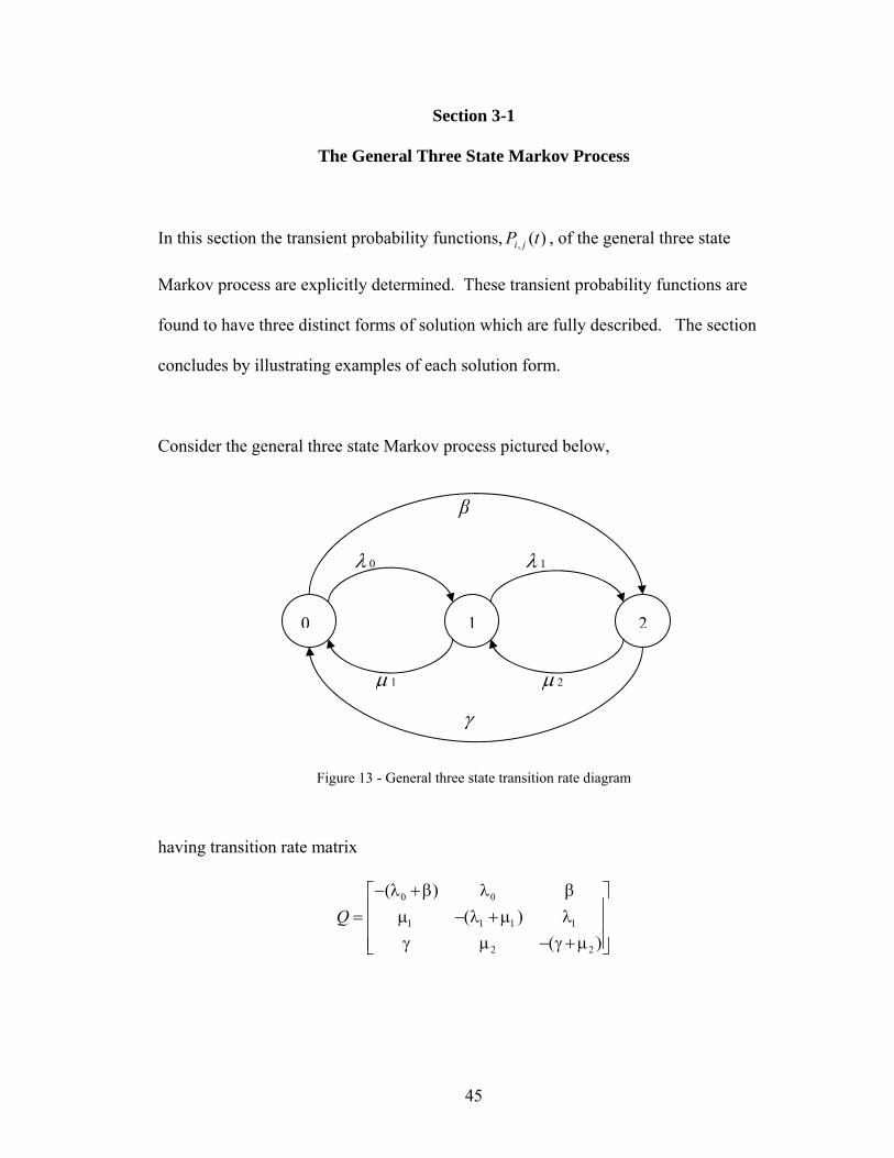
Consider the general three state Markov process pictured below,
γ
μ 1
λ 0 λ 1
μ 2
0 21
β
Figure 13 - General three state transition rate diagram
having transition rate matrix
( ))
)Q
0 0
1 1 1 1
2 2
− λ +β λ β⎡ ⎤⎢ ⎥= μ −(λ +μ λ⎢ ⎥⎢ ⎥γ μ −(γ +μ⎣ ⎦
45

We also denote each entry of Q by , the transition rate of moving from state i to state
j. According to the theory of Markov processes,
jiq ,
0)(
=′=
tijij tPq
for i,j = 0, 1, 2, 3. The matrix Q will also be written as
⎥⎥⎥
⎦
⎤
⎢⎢⎢
⎣
⎡=
2,21,20,2
2,11,10,1
2,01,00,0
qqqqqqqqq
Q
Moving from state zero to state one, for example occurs at a rate 0λ = , and moving
from state zero to state two occurs at rate β = . Since no other transitions out of state
zero occur the rate of staying in state zero is the negative sum of the departing rates, [4],
that is,
1,0q
2,0q
( )βλ +− 0 = . The rows of Q add up to zero. Diagonal entries are non-
positive. Off diagonal terms are non-negative. We are interested in finding the transition
probability functions, , where i , j = 0,1,2. is found by solving the
Kolmogorov forward or backwards equations,
0,0q
)(, tP ji )(, tP ji
QtPtPQtP ⋅=⋅=′ )()()(
with , where I)0( =P
⎥⎥⎥
⎦
⎤
⎢⎢⎢
⎣
⎡=
)()()()()()()()()(
)(
2,21,20,2
2,11,10,1
2,01,00,0
tPtPtPtPtPtPtPtPtP
tP
is the matrix of transition probability functions and Q is as above. The solution of the
Kolmogorov backwards equation can be written [4] as
46

QtetP =)(
and the steady state distribution is given by the following distribution.
Lemma 3-1.1 The steady state distribution of the general three state Markov process
pictured in Figure 13 is
C
C
C
11102
20201
11210
βμβλλλπ
βμγλμλπ
γμγλμμπ
++=
++=
++=
where
122010110211 )()( μμμλλλμλλγμμλβ ++++++++=C
Proof
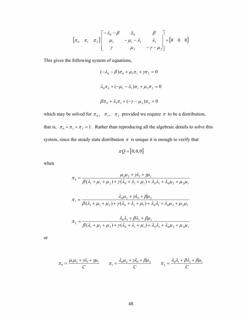
The stationary (and steady state) distribution π may be found see [3] or [4] by solving
[ ]000=Qπ
or
47
[ ] [ 000
22
1111
00
210 =⎥⎥⎥
⎦
⎤
⎢⎢⎢
⎣
⎡
−−−−
−−
μγμγλλμμβλβλ
πππ ]
This gives the following system of equations,
0)(
0)(
0)(
22110
2211100
21100
=−−++
=+−−+
=++−−
πμγπλβπ
πμπλμπλ
γππμπβλ
which may be solved for 210 ,, πππ provided we require π to be a distribution,
that is, 1210 =++ πππ . Rather than reproducing all the algebraic details to solve this
system, since the steady state distribution π is unique it is enough to verify that
[ ]0,0,0=Qπ
when
122010110211
11102
122010110211
20201
122010110211
11210
)()(
)()(
)()(
μμμλλλμλλγμμλββμβλλλ
π
μμμλλλμλλγμμλββμγλμλ
π
μμμλλλμλλγμμλβγμγλμμ
π
++++++++++
=
++++++++++
=
++++++++++
=
or
CCC1110
22020
11121
0βμβλλλπβμγλμλπγμγλμμπ ++
=++
=++
=
48

where
122010110211 )()( μμμλλλμλλγμμλβ ++++++++=C
This straight forward check is left to the reader and completes the proof.
Since the solutions to QtPtPQtP ⋅=⋅=′ )()()( , are known, [13], to have the form
trij
trij
trijij ebeaectP 210)( ++=
when are distinct eigenvalues of Q with constant coefficients (and solution
form when, for example, is a double root), we now turn
our attention to finding the eigenvalues of Q. To determine the eigenvalues of Q, recall
that the characteristic equation of Q is
210 ,, rrr
trij
trij
trijij tebeaectP 110)( ++= 1r
[ ]
0det
0det
22
1111
00
=⎥⎥⎥
⎦
⎤
⎢⎢⎢
⎣
⎡
−−−−−−
−−−
=−
xx
x
xIQ
μγμγλλμμβλβλ
Notice that vector is an eigenvector of Q since . This follows since each
of the rows of Q add up to zero. Thus 0 is an eigenvalue of Q. This means the
characteristic equation of Q may be written as
⎥⎥⎥
⎦
⎤
⎢⎢⎢
⎣
⎡
111
⎥⎥⎥
⎦
⎤
⎢⎢⎢
⎣
⎡=
⎥⎥⎥
⎦
⎤
⎢⎢⎢
⎣
⎡⋅
000
111
Q
0)( 2 =++ CBxxx
where
49
122010110211
2110
)()( μμμλλλμλλγμμλβ
μμλλγβ
++++++++=
+++++=
C
B
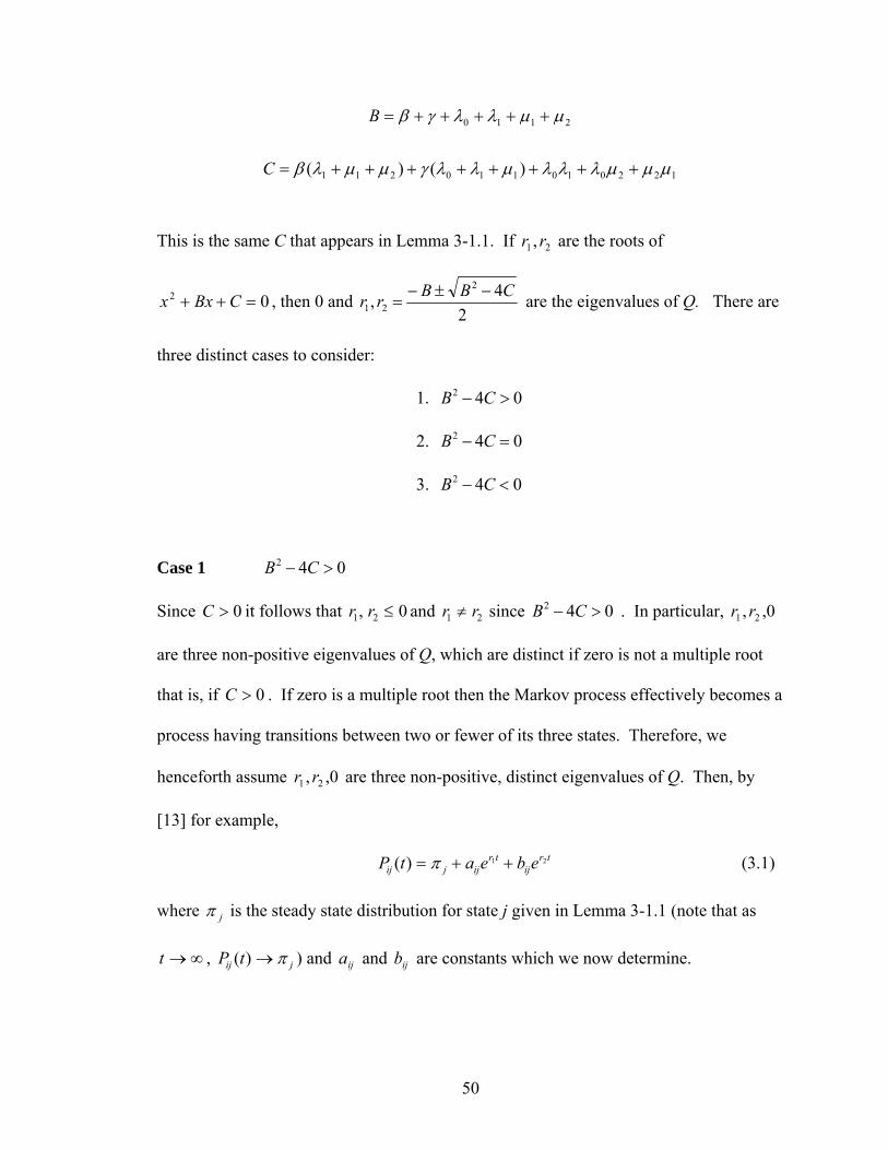
This is the same C that appears in Lemma 3-1.1. If are the roots of
, then 0 and
21, rr
02 =++ CBxx2
4,2
21CBBrr −±−
= are the eigenvalues of Q. There are
three distinct cases to consider:
1. 2 4 0B C− >
2. 2 4 0B C− =
3. 2 4 0B C− <
Case 1 2 4 0B C− >
Since it follows that 0>C 0, 21 ≤rr and 21 rr ≠ since 2 4B C 0− > . In particular,
are three non-positive eigenvalues of Q, which are distinct if zero is not a multiple root
that is, if . If zero is a multiple root then the Markov process effectively becomes a
process having transitions between two or fewer of its three states. Therefore, we
henceforth assume are three non-positive, distinct eigenvalues of Q. Then, by
[13] for example,
0,, 21 rr
0>C
0,, 21 rr
trij
trijjij ebeatP 21)( ++= π (3.1)
where jπ is the steady state distribution for state j given in Lemma 3-1.1 (note that as
, ∞→t jij tP π→)( ) and and are constants which we now determine. ija ijb
50

Substituting t = 0 into equation (3.1) produces,
ijijjijij baP ++== πδ)0(
or ijijjij ba +=−πδ
where is the Kronecker delta function ⎭⎬⎫
⎩⎨⎧
=≠
=jiji
ij for1for0
δ
For any specific , 2,1,0, =ji
0201021)(
===+=′=
t
trijt
trijtijij erberatPq
or 21 rbraq ijijij +=
Then and 21 rbraq ijijij += ijijjij ba +=−πδ can be used to determine and : ija ijb
)()(
)()(
)()(
21
22
21
11
21
1
1
2
rrrq
arrr
qrraq
rrqr
bbr
rbq
jijijij
ijjijijij
ijjijijij
ijijjij
−
−−=→⎥
⎦
⎤⎢⎣
⎡−
−−+=
−
−−=→+
−=−
πδπδ
πδπδ
In summary, becomes, for Case 1, trij
trijjij ebeatP 21)( ++= π 2 4 0B C− >
trijjijtrjijijjij e
rrqr
err
rqtP 21
)()(
)()(
)(21
1
21
2⎥⎦
⎤⎢⎣
⎡−
−−+⎥
⎦
⎤⎢⎣
⎡−
−−+=
πδπδπ
51

with
C
C
C
11102
20201
11210
βμβλλλπ
βμγλμλπ
γμγλμμπ
++=
++=
++=
122010110211
2110
)()( μμμλλλμλλγμμλβ
μμλλγβ
++++++++=
+++++=
C
B
24,
2
21CBBrr −±−
=
where the ijδ and are all known. ijq
Case 2 , double root 2 4B C− = 0
In this case,
220
242 BBCBBr −
=±−
=−±−
=
are double roots of the characteristic equation, where 0<r and
2110 μμλλγβ +++++=B .
The transient probability functions for double roots are (see [14]),
rtij
rtijjij tedectP ++= π)( (3.2)
52
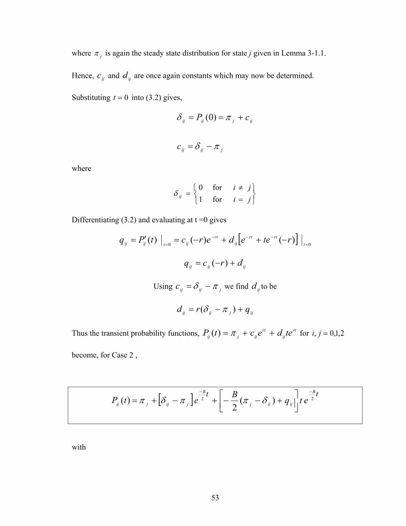
where jπ is again the steady state distribution for state j given in Lemma 3-1.1.
Hence, and are once again constants which may now be determined. ijc ijd
Substituting into (3.2) gives, 0=t
jijij
ijjijij
c
cP
πδ
πδ
−=
+== )0(
where
⎭⎬⎫
⎩⎨⎧
=≠
=jiji
ij for1for0
δ
Differentiating (3.2) and evaluating at t =0 gives
[ ]00
)()()(=
−−−
=−++−=′=
trtrt
ijrt
ijtijij rteederctPq
ijijij drcq +−= )(
Using jijijc πδ −= we find to be ijd
ijjijij qrd +−= )( πδ
Thus the transient probability functions, rtij
rtijjij tedectP ++= π)( for
become, for Case 2 ,
2,1,0, =ji
[ ] tt B
ijijj
B
jijjij etqBetP 22 )(2
)(−−
⎥⎦⎤
⎢⎣⎡ +−−+−+= δππδπ
with
53

C
C
C
11102
20201
11210
βμβλλλπ
βμγλμλπ
γμγλμμπ
++=
++=
++=
122010110211
2110
)()( μμμλλλμλλγμμλβ
μμλλγβ
++++++++=
+++++=
C
B
where ijδ and are all known. ijq
Case 3 2 4 0B C− <
Here,
24
2
24,
2
2
21
BCiB
CBBrr
−±
−=
−±−=
where
122010110211
2110
)()( μμμλλλμλλγμμλβ
μμλλγβ
++++++++=
+++++=
C
B
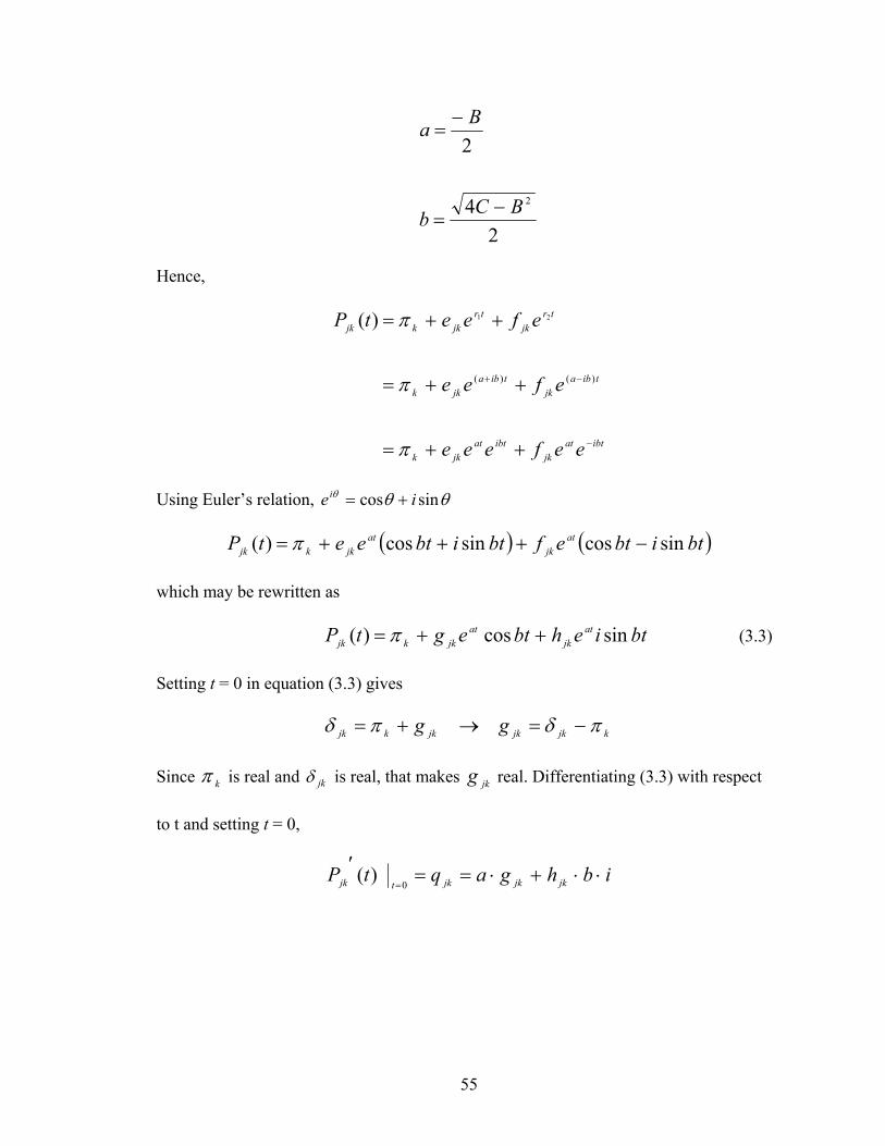
Let and ibar +=1 ibar −=2 where
54
24
2
2BCb
Ba
−=
−=
Hence,
ibtatjk
ibtatjkk
tibajk
tibajkk
trjk
trjkkjk
eefeee
efee
efeetP
−
−+
++=
++=
++=
π
π
π
)()(
21)(
Using Euler’s relation, θθθ sincos iei +=
( ) ( )btibtefbtibteetP atjk
atjkkjk sincossincos)( −+++= π
which may be rewritten as
btiehbtegtP atjk
atjkkjk sincos)( ++= π (3.3)
Setting t = 0 in equation (3.3) gives
kjkjkjkkjk gg πδπδ −=→+=
Since kπ is real and jkδ is real, that makes real. Differentiating (3.3) with respect jkg
to t and setting t = 0,
ibhgaqtP jkjkjktjk ⋅⋅+⋅==′=0
)(
55

But we know is real, is real, is real, and i is the imaginary unit so that makes
pure imaginary, since otherwise we would get a complex number for the
transition rate which can’t happen. So,
jkq jkg b
jkh jkq
jkjkjk qgaibh −⋅=⋅⋅−
jkjkjk qigaibh ⋅−⋅⋅=⋅
bqigai
h jkjkjk
⋅−⋅⋅=
( )⎥⎦
⎤⎢⎣
⎡ −−⋅=
bqa
ih jkkjkjk
πδ
Thus,
( ) ( )
( ) ( )
( ) ( )
( ) ( )⎟⎟⎠
⎞⎜⎜⎝
⎛ −⎥⎦
⎤⎢⎣
⎡
−
−+
−+⎟
⎟⎠
⎞⎜⎜⎝
⎛ −−+=
⎥⎦
⎤⎢⎣
⎡ −⋅−+−+=
⎥⎦
⎤⎢⎣
⎡ −−⋅−−+=
⎥⎥⎦
⎤
⎢⎢⎣
⎡⎥⎦
⎤⎢⎣
⎡ −−⋅+−+=
++=
−−tBCe
BC
B
BC
qtBCe
bteb
aqbte
bteb
qabte
btieb
qaibteA
btiehbtegtP
tB
kjkjktB
kjkk
atkjkjkatkjkk
atjkkjkatkjkk
atjkkjkatkjkk
atjk
atjkkjk
24sin
44
22
4cos
sincos
sincos
sincos
sincos)(
22
22
22
πδπδπ
πδπδπ
πδπδπ
πδδπ
π
56

Thus the transient probability function, for Case 3, 2 4 0B C− < is
[ ] ( )⎟⎟⎠
⎞⎜⎜⎝
⎛
⎥⎥⎦
⎤
⎢⎢⎣
⎡⎟⎟⎠
⎞⎜⎜⎝
⎛= −−
−
−+
−+
−−−+ tBCtB
eBC
kjkB
BC
jkqtBCtB
ekjkktPjk 2
24sin22424
2
2
24cos2)(πδ
πδπ
with
C
C
C
11102
20201
11210
βμβλλλπ
βμγλμλπ
γμγλμμπ
++=
++=
++=
122010110211
2110
)()( μμμλλλμλλγμμλβ
μμλλγβ
++++++++=
+++++=
C
B
where ijδ and are all known. ijq
In summary, the transient probability functions for the general three state Markov process
with transition rate matrix
( ))
)Q
0 0
1 1 1 1
2 2
− λ +β λ β⎡ ⎤⎢ ⎥= μ −(λ +μ λ⎢ ⎥⎢ ⎥γ μ −(γ +μ⎣ ⎦
are given by
57

Case 1 For 2 4 0B C− >
trijjijtrjijijjij e
rrqr
err
rqtP 21
)()(
)()(
)(21
1
21
2⎥⎦
⎤⎢⎣
⎡−
−−+⎥
⎦
⎤⎢⎣
⎡−
−−+=
πδπδπ
Case 2 For 2 4 0B C− =
[ ] tt B
ijijj
B
jijjij etqBetP 22 )(2
)(−−
⎥⎦⎤
⎢⎣⎡ +−−+−+= δππδπ
Case 3 For 2 4 0B C− <
[ ] ( )⎟⎟⎠
⎞⎜⎜⎝
⎛⎥⎦
⎤⎢⎣
⎡⎟⎟⎠
⎞⎜⎜⎝
⎛= −−
−
−+
−+
−−−+ tBCtB
eBC
kjkB
BC
jkqtBCtB
ekjkktPjk 2
24sin22424
2
2
24cos2)(πδ
πδπ
with
C
C
C
11102
20201
11210
βμβλλλπ
βμγλμλπ
γμγλμμπ
++=
++=
++=
122010110211
2110
)()( μμμλλλμλλγμμλβ
μμλλγβ
++++++++=
+++++=
C
B
24,
2
21CBBrr −±−
=
where ijδ and are all known. ijq
58

Examples
Example 1
Case 1 2 4 0B C− >
γ = 2
μ 1 = 1
λ 0 = 1 λ 1 = 1
μ 2 = 1
0 21
β = 2
Figure 14
Here,
3 1 21 2 12 1 3
Q−⎡ ⎤⎢ ⎥= −⎢ ⎥⎢ ⎥−⎣ ⎦
and
[ ]2 24 8 4 2 3 2 3 364 60 4
B C− = − ⋅ + ⋅ +
− =
So the roots are,
1 28 2 , 32
r r − ±= = − , 5−
The steady state distribution is
59
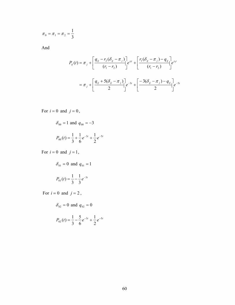
31
210 === πππ
And
tijjijtjijijj
trijjijtrjijijjij
eq
eq
err
qre
rrrq
tP
53
21
1
21
2
2)(3
2)(5
)()(
)()(
)( 21
−−⎥⎦
⎤⎢⎣
⎡ −−−+⎥
⎦
⎤⎢⎣
⎡ −++=
⎥⎦
⎤⎢⎣
⎡−
−−+⎥
⎦
⎤⎢⎣
⎡−
−−+=
πδπδπ
πδπδπ
For and , 0=i 0=j
100 =δ and 300 −=q
tt eetP 5300 2
161
31)( −− ++=
For and , 0=i 1=j
001 =δ and 101 =q
tetP 301 3
131)( −−=
For and , 0=i 2=j
002 =δ and 002 =q
tt eetP 5302 2
165
31)( −− +−=
60
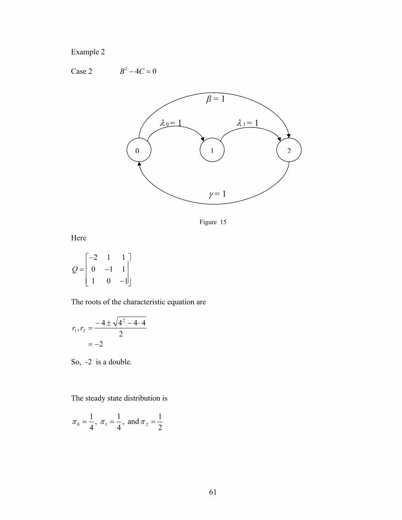
Example 2
Case 2 2 4 0B C− =
γ = 1
λ 0 = 1 λ 1 = 1
0 21
β = 1
Figure 15
Here
2 1 10 1 11 0 1
Q−⎡ ⎤⎢ ⎥= −⎢ ⎥⎢ ⎥−⎣ ⎦
The roots of the characteristic equation are
22
4444,2
21
−=
⋅−±−=rr
So, -2 is a double.
The steady state distribution is
21 and ,
41 ,
41
210 === πππ
61

with and 4=C 4=B
and
[ ]
[ ] [ ] tetqte
tetqBt
etP
ijijjjijj
B
ijijj
B
jijjij
2)(22
)(2
)( 22
−+−−+−−+=
⎥⎦⎤
⎢⎣⎡ +−−+−+=
−−
δππδπ
δππδπ
For and , 0=i 0=j
100 =δ and 200 −=q
tt teetP 2200 2
143
41)( −− −+=
For and , 0=i 1=j
001 =δ and 101 =q
tt teetP 2201 2
141
41)( −− +−=
For and , 0=i 2=j
002 =δ and 102 =q
tt teetP 2202 2
21
21)( −− +−=
62
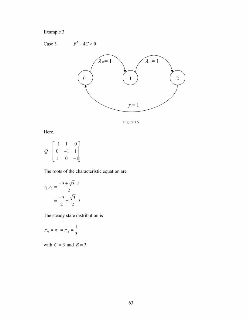
Example 3
Case 3 2 4 0B C− <
γ = 1
λ 0 = 1 λ 1 = 1
0 21
Figure 16
Here,
1 1 00 1 11 0 1
Q−⎡ ⎤⎢ ⎥= −⎢ ⎥⎢ ⎥−⎣ ⎦
The roots of the characteristic equation are
i
irr
⋅±−
=
⋅±−=
23
23
233, 21
The steady state distribution is
31
210 === πππ
with and 3=C 3=B
63

[ ] ( )
⎟⎟⎠
⎞⎜⎜⎝
⎛−
⎥⎥⎥⎥
⎦
⎤
⎢⎢⎢⎢
⎣
⎡⎟⎠⎞
⎜⎝⎛ −
++⎟⎟⎠
⎞⎜⎜⎝
⎛−⎥⎦⎤
⎢⎣⎡ −+=
⎟⎟⎟
⎠
⎞
⎜⎜⎜
⎝
⎛ −−
⎥⎥
⎦
⎤
⎢⎢
⎣
⎡
−
−+
−+
⎟⎟⎟
⎠
⎞
⎜⎜⎜
⎝
⎛ −−−+=
tt
ejkjkq
tt
ejk
tBCtB
eBC
kjkB
BC
jkqtBCtB
ekjkktPjk
23sin2
3
3313
3
2
23cos2
3
31
31
2
24sin22424
2
2
24cos2)(
δδ
πδπδπ
For and , 0=j 0=k
100 =δ and 100 −=q
⎟⎟⎠
⎞⎜⎜⎝
⎛⎟⎠⎞
⎜⎝⎛+=
−tetP
t
23cos
32
31)( 2
3
00
For and , 0=j 1=k
001 =δ and 101 =q
⎟⎟⎠
⎞⎜⎜⎝
⎛+⎟⎟
⎠
⎞⎜⎜⎝
⎛−=
−−tetetP
tt
23sin
31
23cos
31
31)( 2
323
01
For and , 0=j 2=k
002 =δ and 002 =q
⎟⎟⎠
⎞⎜⎜⎝
⎛−⎟⎟
⎠
⎞⎜⎜⎝
⎛−=
−−tetetP
tt
23sin
31
23cos
31
31)( 2
323
02
64
Conclusion
In this thesis, ruin probabilities are determined for the gambler’s ruin with catastrophes
and windfalls. For the finite time problem, lattice path combinatorics described in
Chapter 1 play a key role in determining the ruin probabilities by providing us a formula
for counting sample paths of the Markov chain. In the infinite time case (Chapter 2), the
ruin probability recurrence relations have been solved using probability generating
functions and the theory of difference equations. These problems generalize and include
the well-known, classical gambler’s ruin problem as a special case of the solutions
developed within this thesis. A preliminary literature search indicates that the solutions
determined in this thesis appear new. However, the gambler’s ruin problem dates back so
many years (over three centuries) that a more extensive literature search still needs to be
undertaken. At the same time, further generalizations of the gambler’s ruin problems
have been progressing at Cal Poly Pomona, see, for example [5] where ruin probabilities
having state dependent probabilities are being studied. The gambler’s ruin may also be
extended along the lines of a batch queueing system, that is, having a transition diagram
where a player moves down by two steps instead of one step.
In Chapter 3, the transient probability functions of the general three state Markov process
is determined. Our method of solution involves obtaining general, explicit formulae for
the eigenvalues of Q and the steady state distribution of the three state Markov process.
After this, a categorization of the (distinct) solution function forms is given in Chapter 3.
65
Even though this approach to determining transient probability functions is well known,
so far, we have not seen the solution of the three state Markov process carried out in such
complete generality. Our general solution raises some interesting questions that are not
yet completely understood. For example, why does the quantity
122010110211 )()( μμμλλλμλλγμμλβ ++++++++=C
appear in both the steady state distribution of the system and the eigenvalues of Q ?
What is the significance of C? The hope is that our general form of solution reveals new
insights into the patterns of how transient probability functions look in general. The next
step of future research might be to perform a similar analysis for the four state Markov
process. The eigenvalues of Q once again may be determined explicitly in terms of the
entries of Q -this time by using the formula for the roots of a cubic equation. The steady
state distribution is again solvable but not obvious. Since the four state Markov process
contains the three and two state Markov process as special cases, again one may hope to
learn more about how the general N-state Markov process transient probability looks. In
short, the range of future work on this topic is endless.
66
References
[1] Edwards, A.W.F, Pascal’s Problem: The ‘Gambler’s Ruin’,
International Statistical Review, 73-79, 1983.
[2] Goldberg, S., Introduction to Difference Equations, with
Illustrative Examples from Economics, Psychology, and Sociology,
Dover Publications, Inc., New York, 1986.
[3] Gross, D and Harris, C.M., Fundamentals of Queueing Theory,
Second Edition, John Wiley and Sons, New York, 1985.
[4] Hoel, P., Port, S., and Stone C., Introduction to Stochastic
Processes, Waveland Press Inc., 1987.
[5] Hunter, B., Krinik, A., Nguyen, C., Switkes, J., von Bremen, H.,
Approaches to Gambler’s Ruin with Catastrophe, (preprint).
[6] Kasfy, H., Dual Processes to Determine Transient Probability
Functions, Masters Thesis, Cal Poly Pomona, 2004.
[7] Krinik, A., Rubino, G., Marcus, D., Swift, R., Kasfy, H., Lam, H.,
Dual Processes to Solve Single Server Systems, Journal of
Statistical Planning and Inference, 135, Special Issue on Lattice
Path Combinatorics and Discrete Distributions, 121-147, 2005.
67

[8] Marcus, D., Combinatorics: A Problem Oriented Approach, The
Mathematical Association of America, Washington, 1998.
[9] Mohanty, S. G., Lattice Path Counting and Applications, Academic
Press, 1979.
[10] Narayana, T.V., Lattice Path Combinatorics With Statistical
Applications, University of Toronto Press, Toronto, 1979.
[11] Takacs, L., On The Classical Ruin Problems, JASA, 64, 889-906,
1969.
[12] Wilf, H., Generatingfunctionology, Academic Press, Inc., 1994.
[13] Zill, D., A First Course in Differential Equations with Modeling
Applications, 6th Edition, Brooks/Cole Publishing, 1997.
68