gama/wigglez: the 1.4 ghz radio luminosity functions of ...400920/uq400920_oa.pdf · power law....

MNRAS 460, 2–17 (2016) doi:10.1093/mnras/stw910Advance Access publication 2016 April 20

GAMA/WiggleZ: the 1.4 GHz radio luminosity functions of high- andlow-excitation radio galaxies and their redshift evolution to z = 0.75

Michael B. Pracy,1‹ John H. Y. Ching,1 Elaine M. Sadler,1 Scott M. Croom,1

I. K. Baldry,2 Joss Bland-Hawthorn,1 S. Brough,3 M. J. I. Brown,4 Warrick J. Couch,3

Tamara M. Davis,5 Michael J. Drinkwater,5 A. M. Hopkins,3 M. J. Jarvis,6,7

Ben Jelliffe,1 Russell J. Jurek,8 J. Loveday,9 K. A. Pimbblet,10,11 M. Prescott,7

Emily Wisnioski12 and David Woods13

1Sydney Institute for Astronomy, School of Physics, University of Sydney, NSW 2006, Australia2Astrophysics Research Institute, Liverpool John Moores University, IC2, Liverpool Science Park, 146 Brownlow Hill, Liverpool L3 5RF, UK3Australian Astronomical Observatory, PO Box 915, North Ryde, NSW 1670, Australia4School of Physics and Astronomy, Monash University, Clayton, VIC 3800, Australia5School of Mathematics and Physics, University of Queensland, Brisbane, QLD 4072, Australia6Oxford Astrophysics, Department of Physics, Keble Road, Oxford OX1 3RH, UK7Astrophysics Group, Department of Physics, University of the Western Cape, Bellville 7535, South Africa8Australia Telescope National Facility, CSIRO, Epping, NSW 1710, Australia9Astronomy Centre, University of Sussex, Falmer, Brighton BN1 9QH, UK10E.A. Milne Centre for Astrophysics and Department of Physics and Mathematics, University of Hull, Cottingham Road, Kingston-upon-Hull HU6 7RX, UK11School of Physics, Monash University, Clayton, VIC 3800, Australia12Max Planck Institut fur extraterrestrische Physik, GiessenbachstraIse, D-85748 Garching, Germany13Department of Physics and Astronomy, University of British Columbia, 6224 Agricultural Road, Vancouver, BC V6T 1Z1, Canada

Accepted 2016 April 15. Received 2016 April 14; in original form 2015 December 24

ABSTRACTWe present radio active galactic nuclei (AGN) luminosity functions over the redshift range0.005 < z < 0.75. The sample from which the luminosity functions are constructed is anoptical spectroscopic survey of radio galaxies, identified from matched Faint Images of theRadio Sky at Twenty-cm survey (FIRST) sources and Sloan Digital Sky Survey images.The radio AGN are separated into low-excitation radio galaxies (LERGs) and high-excitationradio galaxies (HERGs) using the optical spectra. We derive radio luminosity functions forLERGs and HERGs separately in the three redshift bins (0.005 < z < 0.3, 0.3 < z < 0.5and 0.5 < z < 0.75). The radio luminosity functions can be well described by a doublepower law. Assuming this double power-law shape the LERG population displays little or noevolution over this redshift range evolving as ∼(1 + z)0.06+0.17

−0.18 assuming pure density evolutionor ∼(1 + z)0.46+0.22

−0.24 assuming pure luminosity evolution. In contrast, the HERG populationevolves more rapidly, best fitted by ∼(1 + z)2.93+0.46

−0.47 assuming a double power-law shape andpure density evolution. If a pure luminosity model is assumed, the best-fitting HERG evolutionis parametrized by ∼(1 + z)7.41+0.79

−1.33 . The characteristic break in the radio luminosity functionoccurs at a significantly higher power (�1 dex) for the HERG population in comparison tothe LERGs. This is consistent with the two populations representing fundamentally differentaccretion modes.

Key words: galaxies: active – radio continuum: galaxies.

1 IN T RO D U C T I O N

The evolution of galaxies and the supermassive black holes at theircentres appear to be closely connected. This connection is evident

�E-mail: [email protected]

in the correlation between black hole mass and the stellar bulgemass (Magorrian et al. 1998) and black hole mass and stellar ve-locity dispersion (e.g. Gebhardt et al. 2000). One way this couplingmay occur is via feedback processes from the active galactic nuclei(AGN) depositing energy, released by the accretion of matter on tothe black hole, into their host galaxy and its surrounding environ-ment. For example, radio jets from AGN are commonly invoked as

C© 2016 The AuthorsPublished by Oxford University Press on behalf of the Royal Astronomical Society

at UQ

Library on A

ugust 22, 2016http://m

nras.oxfordjournals.org/D

ownloaded from

mailto:[email protected]

http://mnras.oxfordjournals.org/

The 1.4 GHz radio luminosity function 3

a feedback mechanism to inhibit gas cooling and suppress star for-mation in massive galaxies and clusters of galaxies (e.g. Binney &Tabor 1995; Fabian et al. 2002; Best et al. 2006; Bower et al. 2006;Croton et al. 2006; McNamara & Nulsen 2007). Such a feedbackcycle can simultaneously solve the cooling flow problem; the sharpbright-end turn down in the optical galaxy luminosity function andthe fact that the most massive bulge-dominated galaxies contain theoldest stellar populations (Croton et al. 2006).

The properties of the AGN population indicate that there aretwo fundamentally different accretion modes operating (Hardcas-tle, Evans & Croston 2007; Best & Heckman 2012). In the classical‘cold mode’, material is accreted on to the supermassive blackhole via a small, geometrically thin, optically luminous accretiondisc. This disc is the source of ionizing photons producing bothbroad- and narrow-line emission in the optical spectrum of AGNand X-ray emission via the inverse-Compton process. In the unifiedAGN model (Antonucci 1993), the broad-line region is obscuredby a dusty torus when viewed from certain orientations resultingin the type I (not obscured) and type II (obscured) AGN classifi-cations. As a result of the emission lines in their optical spectra,these ‘cold-mode’ AGN are also referred to as ‘quasar-mode’ or‘high-excitation’ AGN. However, there is a large population ofAGN observable by their radio emission but without the brighthigh-ionization emission lines in their optical spectra (e.g. Hine &Longair 1979; Laing et al. 1994; Jackson & Rawlings 1997; Best &Heckman 2012). These display no evidence for the presence of anaccretion disc or dusty torus (e.g. Chiaberge et al. 2002; Whysong& Antonucci 2004) and are likely powered by radiatively inefficientaccretion possibly from a hot gas halo (e.g. Hardcastle et al. 2007;Best & Heckman 2012). These ‘hot-mode’ AGN (also referred toas ‘radio-mode’ or ‘low-excitation’ AGN) are generally more mas-sive, have higher mass-to-light ratios, are redder, and are of earliermorphological type than strong-lined AGN (e.g. Kauffmann et al.2003; Kauffmann, Heckman & Best 2008; Best & Heckman 2012).The ‘cold-mode’ AGN display a higher rate of interactions andpeculiarities in their morphology (e.g. Smith & Heckman 1989).

Both AGN modes will inject energy into their environment andhave the potential to influence star formation and galaxy evolu-tion. In the ‘hot mode’ the radio jets heat the surrounding hot gasatmosphere. This is the same gas that fuels the AGN allowing aself-regulating feedback cycle with a balance established betweenheating and cooling (Best et al. 2006; Croton et al. 2006). In the‘cold-mode’ AGN are known to drive winds in their host galaxy(e.g. Ganguly & Brotherton 2008; Harrison et al. 2014; McElroyet al. 2015) and have been suggested as mechanisms to both en-hance (Silk & Nusser 2010) and suppress (Shabala, Kaviraj & Silk2011; Davis et al. 2012; Page et al. 2012) star formation.

In the local Universe, the number of radio AGN with low-excitation optical spectra (low-excitation radio galaxies, hereafterLERGs) outnumber the high-excitation radio galaxies (hereafterHERGs) at all but the highest radio luminosities (Best & Heckman2012). The change in the dominant population occurs at L1.4 GHz

∼ 1026 W Hz−1. The cosmic evolution of the space density of ra-dio AGN is sensitive to radio luminosity. It is well established thatthe density of the most powerful radio AGN increases rapidly withincreasing redshift out to z ∼ 2 (Longair 1966; Doroshkevich, Lon-gair & Zeldovich 1970; Willott et al. 2001; Sadler et al. 2007)– increasing by a factor of ∼1000. At higher redshift the spacedensity flattens and then decreases. The decrease occurs at higherredshift for more luminous sources (e.g. Peacock 1985; Dunlop& Peacock 1990; Cirasuolo et al. 2006). This fast-evolving high-luminosity population is mostly associated with Fanaroff–Riley II

radio sources (Jackson & Wall 1999) and objects with strong op-tical emission lines (Willott et al. 2001; Best & Heckman 2012),i.e. HERGs. Conversely, the low-luminosity radio sources are morecommonly associated with Fanaroff–Riley I sources and objectswhich lack strong optical emission lines, i.e. LERGs. The spacedensity of these low-luminosity radio galaxies shows little (a factorof ∼2) or no redshift evolution out to z ∼ 1 (e.g. Clewley & Jarvis2004; Sadler et al. 2007; Donoso, Best & Kauffmann 2009; Smolcicet al. 2009; McAlpine, Jarvis & Bonfield 2013).

Best & Heckman (2012) constructed the first radio galaxy lumi-nosity function with the LERG and HERG contributions separated.They found, that while the LERGs outnumber the HERGs belowL1.4 GHz ∼ 1026 W Hz−1, examples of both classes are found at allradio luminosities. The HERG population shows evidence of evo-lution over the redshift range of their sample (z < 0.3), while thereis no evidence for cosmic evolution of the LERG population. Thisimplies the evolution of the radio luminosity functions dependenceon radio luminosity can, at least in part, be explained by a changingmix in the populations (Best & Heckman 2012). Best et al. (2014)using a composite of eight published AGN samples (Wall & Peacock1985; Lacy et al. 1999; Waddington et al. 2001; Hill & Rawlings2003; Simpson et al. 2006; Gendre, Best & Wall 2010; Rigby et al.2011) constructed a catalogue of 211 radio-loud AGN in the range0.5 < z < 1.0. Using this to compare with local samples (Best &Heckman 2012; Heckman & Best 2014) they made the first mea-surement of the evolution of the radio AGN population separated,spectroscopically, into LERGs (jet mode in their nomenclature) andHERGs (dubbed radiative mode). They found that the space densityof the HERGs in their sample increased by around an order of mag-nitude to z = 1. In contrast, the LERG AGN density decreased withredshift at luminosities below L1.4 GHz ∼ 1026 W Hz−1 and increasedat higher luminosities.

In this paper, we present the radio luminosity function of LERGsand HERGs and their cosmic evolution to z = 0.75, correspondingto the second half of the history of the Universe. These luminosityfunctions are based on a new sample of over 5000 radio galaxies(0.005 < z < 0.75) with confirmed spectroscopic redshifts andspectroscopic classifications. Throughout this paper, we convertfrom observed to physical units assuming a �M = 0.3, �� = 0.7and H0 = 70 km s−1 Mpc−1 cosmology.

2 SA M P L E C O N S T RU C T I O N

The underlying sample from which we constructed the luminositydistributions of various radio galaxy populations is the Large AreaRadio Galaxy Evolution Spectroscopic Survey (Ching 2015). Thissample was constructed by matching the Faint Images of the RadioSky at Twenty-cm survey (FIRST; Becker, White & Helfand 1995)with the photometric catalogue of the Sloan Digital Sky Survey datarelease 6 (SDSS; Adelman-McCarthy et al. 2008). The catalogueswere matched to all objects in the FIRST catalogue (�0.5 mJy) andan optical apparent magnitude limit of i = 20.5 (SDSS i-band modelmagnitudes). The matching procedure was designed to include bothpoint and extended radio sources, including those with multiplecomponents. This matching was performed over ∼900 deg2 of skyin regions where a high completeness of optical spectroscopy couldbe obtained. A careful estimation of the matching reliability andcompleteness was performed by Ching (2015) using Monte Carlosimulations of randomized catalogues. The overall reliability of thematching is estimated as ∼93.5 per cent and the overall complete-ness is ∼95 per cent. The incompleteness and inclusion of falsematches will somewhat offset in the effects on the normalization

MNRAS 460, 2–17 (2016)

at UQ

Library on A



ownloaded from


4 M. B. Pracy et al.

Figure 1. Number of objects per interval of 1.4 GHz flux density in theparent sample (diamonds). The vertical dashed line shows the flux densitylimit (S1.4 GHz > 2.8 mJy) applied in this paper. The number counts are stillrising at this flux density.

of the luminosity functions. We do not do any scaling of the lumi-nosity functions to account for input catalogue incompleteness butnote that its effect on the normalization could not be more than afew per cent.

A possible systematic could arise if the incompleteness or falsematches are biased towards a particular source type or source prop-erties. The most likely source of such a bias is the behaviour of thematching algorithm for sources with complex (non-point source)radio morphologies. Such sources are more common at low redshiftand lower luminosity as a result of angular resolution effects andthe presence of extended star-forming galaxies. There is no evi-dence for such a bias. Only ∼10 per cent of the sample is matchedto more than one FIRST component, which is consistent with otherdeterminations from the literature (Ivezic et al. 2002). Of those∼10 per cent the fraction of matches to the random catalogues arealmost identical for FIRST sources with two, three and four or morecomponents.

While the high spatial resolution of the FIRST catalogue makesit preferable for matching to the optical photometry it will also re-solve out extended radio emission resulting in lower flux densitymeasurements. Since angular size decreases with redshift this fluxloss will be more significant at low redshift and could mimic evolu-tion in the radio luminosity function. To avoid this, we replace theflux densities with those measured from the lower spatial resolutionNRAO VLA Sky Survey (NVSS; Condon et al. 1998) catalogue. Inthe case where a single NVSS source coincides with more than oneFIRST source the NVSS flux is split between objects with the sameflux ratio as measured by FIRST (see Ching 2015 for details of thematching of FIRST and NVSS sources).

At the faintest flux densities the NVSS catalogue will suffer fromsignificant incompleteness. To avoid working with a parent samplethat suffers from such incompleteness, we only include objects withflux density greater than 2.8 mJy in constructing our luminosityfunction. This is the same flux limit adopted by Sadler et al. (2007)when matching radio sources to the luminous red galaxies in the2dF-SDSS LRG and QSO survey (2SLAQ; Croom et al. 2009).With this flux-density limit the source counts are still rising at thefaintest flux densities; as demonstrated in Fig. 1. This results in asample of 10 827 matched radio/optical sources.

The optical spectroscopy for the sample was gathered either frompublicly available archival sources such as the SDSS (Adelman-

McCarthy et al. 2008), 2SLAQ (Cannon et al. 2006; Croom et al.2009) and the 2dF QSO redshift survey (2QZ; Croom et al. 2004) orfrom a dedicated ‘spare-fibre’ campaign using the 2dF/AAOmegainstrument on the Anglo-Australian Telescope. This was done by‘piggy-backing’ on the WiggleZ Dark Energy Survey (WiggleZ;Drinkwater et al. 2010) and GAMA (Baldry et al. 2010; Driveret al. 2011; Liske et al. 2015) large survey programmes by using asmall number of fibres on each survey field to target radio galaxies(see Ching (2015) for details). This has almost no impact on thelarge survey efficiency but over time results in a large number of‘spare-fibre’ spectra being obtained. Of the 10 827 radio galaxiessatisfying our 1.4 GHz flux density criterion, the number with op-tical spectra is 7088. Of these 6215 are deemed to have reliableredshift determinations (∼87 per cent).

2.1 Optical spectroscopic classification

In addition to providing an accurate measure of the redshift theoptical spectroscopy can be used to determine the physical ori-gin of the radio emission, i.e. star formation or AGN. The opticalspectroscopy can also be used to separate the AGN into LERGsand HERGs. Full details of the semi-automatic classification pro-cedure is given in Ching (2015). In brief, FIRST galaxies whoseradio emission is dominated by star formation are identified usinga Baldwin, Philips and Terlevich (hereafter BPT; Baldwin, Phillips& Terlevich 1981) diagram. Only galaxies with radio luminosityL1.4 GHz ≤ 1024 W Hz−1 and z < 0.3 are considered, since galax-ies more powerful than this would require unrealistically high starformation rates and so are assumed to have their radio emission gen-erated by an AGN. The BPT diagnostic will not work in the casewhere the galaxy has a radio-quiet optical AGN and radio emissionpowered by star formation (Best & Heckman 2012; Ching 2015).These cases were identified based on a comparison of the inferredstar formation rates from H α and radio luminosity. The remainingradio galaxies are classified as AGN and further subdivided usingthe equivalent width of the [O III]λ5007 emission line, where galax-ies are classified as HERGs if they have SNR([O III]λ5007) > 3 andEW([O III]λ5007) > 5 Å. See Ching (2015) for a detailed descrip-tion of the methods used to make the line strength measurements.The 5 Å demarcation is the same as that used by Best & Heckman(2012).

The O [III]λ5007 line is redshifted out of the WiggleZ and SDSSspectra at z ∼ 0.83 and out of the GAMA spectra at z ∼ 0.76. Thesealso correspond, approximately, to the redshift where our opticalk-corrections are expected to be reliable (Blanton & Roweis 2007).In addition, as a result of the magnitude limit of the optical spec-troscopic follow-up, above z ∼ 0.75 the spectroscopic sample isdominated by broad-line AGN and there are almost no narrow-lineAGN or LERGs in the sample (see Fig. 2). We therefore impose aredshift limit of z = 0.75 for construction of our luminosity func-tions. We also apply a lower redshift limit of z = 0.005 to removeGalactic objects. With these cuts the final number of objects, withreliable redshifts, is 5026. A summary of the number of spectrafrom each survey in these final 5026 objects is given in Table 1.Not all objects can be classified using the semi-automated meth-ods of Ching (2015). Out of the 5026 objects in our sample, 284(∼6.7 per cent) were not classified by Ching (2015). A fraction ofthe spectra in the Ching (2015) sample had been inspected andclassified visually, and in the cases where there is no automatedclassification but a visual one, we use this visual classification.This leaves 229 objects (corresponding to ∼4.6 per cent) without aclassification. Rather than carry these unclassified objects through

MNRAS 460, 2–17 (2016)

at UQ

Library on A



ownloaded from



Figure 2. Left-hand panel: the redshift distribution of all radio galaxies with reliable spectroscopic redshifts. The redshift distributions for star-forminggalaxies, LERGs and HERGs are shown separately. Above z ∼ 0.8, the sample is dominated by broad-line AGN. Right-hand panel: the n(z) of the sample usedto construct luminosity functions in this paper after selecting objects with 0.005 < z < 0.75 and S1.4 GHz > 2.8 mJy.

Table 1. A summary of the number of spectra from each survey in thesefinal 5026 objects which are used in the measurement of the luminosityfunctions.

z < 0.3 0.3 ≤ z < 0.5 0.5 ≤ z < 0.75 Total

N(SDSS) 1958 846 221 3025N(WiggleZ main)a 26 137 151 314N(WiggleZ radio)b 72 354 389 815N(WiggleZ other)c 9 15 40 64N(GAMA) 154 298 221 673N(2SLAQ LRGs) 0 32 95 127N(2SLAQ QSOs) 1 1 3 5N(2QZ/6QZ) 1 1 1 3Total 2221 1684 1121 5026

Notes. aWiggleZ main survey targets.bSpare fibre targets for this project.cTarget for other spare fibre programs.

the analysis we performed visual classification of these sources.For the most part this was straightforward. The fraction of objectsclassified as each type visually are similar to the overall fractionsbut with a lower frequency of ‘star-forming’ objects and a higherfraction of HERGs. The fractions of objects of each type prior tothe visual classification are ∼75.2, 14.3 and 10.5 per cent for theLERGs, HERGs and star-forming galaxies, respectively. The cor-responding fractions in the visual classification are ∼78.6, 20.9 and0.5 per cent. The increase in the HERG fraction (including quasars)and the decrease in the star-forming fraction is expected since theredshift distribution of the unclassified objects is, not surprisingly,peaked at the high-redshift end of the sample.

3 T H E R A D I O L U M I N O S I T Y FU N C T I O N

We first wish to construct the bivariate luminosity function for allgalaxies in the optical-radio matched sample in multiple redshiftbins. That is, we calculate the volume density of galaxies per intervalof radio luminosity per interval of optical luminosity in each redshiftbin. To do this we use the standard 1/Vmax method (Schmidt 1968),where the number density in each bin is given by

�(Mi, L1.4 GHz)�Mi� log L1.4 GHz =∑gal

wgal

Vmax(gal). (1)

The sum on the right-hand side is over all galaxies in the bin.The weight, wgal, given to each galaxy corrects for incompletenessin the spectroscopic follow-up. For a complete survey wgal = 1and for incomplete samples wgal is given by the reciprocal of thecompleteness. The denominator, Vmax(gal), is the maximum volumeover which the galaxy could have been observed given the selectionlimits in both the radio and optical. We outline our methods forestimating wgal and Vmax(gal) below.

3.1 Estimating the completeness

The overall spectroscopic completeness is given by the numberof targets for which we obtained a spectrum of sufficient qual-ity to make a reliable redshift measurement divided by the num-ber of targets in the parent radio/optical matched sample. That is6215/10 827 or ∼57 per cent. This is mostly targeting incomplete-ness; the percentage of spectroscopically targeted objects whichresulted in a good quality redshift classification, i.e. spectroscopiccompleteness, is ∼90 per cent. This spectroscopic incompletenessis not random. It will depend sensitively on the optical magnitudefor at least two reasons. First, the optical spectroscopy of the sam-ple is constructed from spectroscopy from multiple surveys, whichhave different limiting magnitudes. In addition, the spectroscopiccompleteness within an individual survey generally decreases withoptical magnitude as the noisier spectra obtained for fainter galaxiesmake it increasingly difficult to identify the redshift. Ching (2015)used repeat observations to demonstrate that there is little differ-ence in the likelihood of obtaining a redshift for different spectralclasses (with and without emission lines) once optical magnitudeis taken into account. They did this by comparing the fraction ofobjects of different spectral classes that required more than onerepeat observation to acquire a good redshift. The idea being thatif for a particular source type it is easier to identify a redshift (atgive apparent magnitude) than it should, on average, require lessrepeat observations. While they did find a slightly higher tendencyfor spectra without emission lines to require a repeat observationthan those with emission lines, it was not statistically significant.One important caveat on this technique is that it can only be usedin cases where a reliable redshift is eventually obtained by one ofthe observations.

The completeness will also be sensitive to colour, again for at leasttwo distinct reasons. First, while most of spectra were obtained

MNRAS 460, 2–17 (2016)

at UQ

Library on A



ownloaded from



Figure 3. The completeness map in the i-magnitude versus g − i colour plane, used to generate the weight (wgal; shown in side bar) assigned to each galaxyin constructing the luminosity function. Overlaid blue points are the photometric sample objects above our 2.8 mJy flux limit for which a reliable redshift hasbeen obtained. The overlaid red points are objects for which no spectroscopic follow-up observation was made. The yellow points represent objects whichwere observed spectroscopically but a reliable redshift could not be determined. The structure in the completeness map, such as the low completeness forfaint objects with g − i colours of ∼1–2 mag, is mostly the result of targeting completeness in the constituent surveys and demonstrates the importance ofconstructing our completeness estimates in this plane.

from surveys that do not apply colour selection criteria (e.g. ourdedicated follow-up, targets with SDSS spectra and the GAMAmain survey), a fraction of the spectra come from surveys that do(e.g. the WiggleZ main survey, 2SLAQ and 2QZ). Another reasoncompleteness will vary with colour, is that colour correlates withother spectral properties which make a redshift easier to identify. Inparticular, galaxies with bluer colour are more likely to have easy toidentify emission lines. Although, as mentioned above, this appearsto cause little bias.

There may be other properties which influence the spectroscopiccompleteness (e.g. changes in the observable spectral features in afixed observing band with redshift) but it is likely that magnitudeand colour account for the dominant dependences. We thereforechoose to construct our spectroscopic completeness in this plane,specifically we calculate our completeness (and hence our wgal’s)in the i-magnitude versus g − i plane.

We calculate the completeness for each object (or position) inthe i-magnitude versus g − i plane by averaging over an adaptively

sized circle in this plane. The size of the circle is calculated byusing the distance in the plane to the 50th nearest neighbour inthe photometric input catalogue. Using this adaptive bin size forestimating the completeness means in regions of the plane with fewobjects we still use a reasonable number of objects in estimatingthe completeness, while in high-density regions we obtain a finermore local sampling of the completeness. The completeness in thisplane is shown in Fig. 3. Each galaxy is assigned a wgal given bythe reciprocal of the completeness. Using this nearest neighbourmethod for estimating the completeness even objects with largeweights have had their completeness estimated using a reasonablenumber of objects. For example, for an object with a weight of 10(completeness of 0.1) the estimate is based on five objects with goodspectra and 50 objects in the input catalogue. We also checked thatour luminosity functions are not largely affected by objects withthe highest weights. Removing objects with weights greater than10 makes no significant quantitative difference and no qualitativedifference to our results.

MNRAS 460, 2–17 (2016)

at UQ

Library on A



ownloaded from



Figure 4. The bivariate luminosity distribution. The space density represented by a colour-scale in the optical magnitude–radio luminosity plane. The panelsare for the different redshift bins: left: 0.005 < z < 0.30; middle: 0.30 < z < 0.50; and right: 0.5 < z < 0.75. The flux-density and apparent magnitude selectionlimits correspond to progressively brighter radio and optical luminosity limits with increasing redshift. The absolute magnitude limit applied when analysingthe redshift evolution of the radio luminosity function is shown as the vertical line. This corresponds to the absolute magnitude limit at the high-redshift edgeof the highest redshift bin not inclusive of an e-correction.

3.2 Estimating Vmax

To evaluate equation (1), and correctly weight the contribution tothe luminosity function of each galaxy in our sample, we needto estimate the volume within which each galaxy would satisfythe optical and 1.4 GHz flux density selection limits, i.e. Vmax.This volume will depend on the redshift of the source, its opticalmagnitude, 1.4 GHz flux density, and the spectral shape in boththe optical and radio regimes. To do this, for each source, we firstcalculate the absolute i-band magnitude including a k-correctionand evolutionary correction:

Mi = mi − DM − Ki(z) − e(z), (2)

where DM is the distance modulus, Ki(z) is the k-correction ande(z) is the evolutionary correction (e-correction). The k-correctionis calculated using version v4_2 of the KCORRECT package (Blanton& Roweis 2007) using the five band (u,g,r,i,z) SDSS photometry.The e-correction accounts for the fading of stellar populations withtime. For the LERGs we use the e-corrections for early-type galaxiesfrom Poggianti (1997). The HERGs are generally bluer, more likelyto be interacting and star-forming (or recently star-forming) systemswhich mitigates the effect on the overall optical luminosity of theageing of the underlying older stellar population. Given this we sete(z) = 0 for the HERGs and discuss the effects this assumptionhas on the evolution of the luminosity function in Section 4. It isworth noting that the magnitude of the e-correction is significant:increasing from ∼0.1 mag (i-band) at z = 0.1 to ∼0.8 mag atz = 0.75.

We then calculate the radio luminosity, also including a k-correction:

L1.4GHz = 4πd2L

1

(1 + z)(1+α)S1.4GHz (3)

here dL is the luminosity distance and α is the spectral index, definedas Sν = να . We assume the canonical α = −0.7 (Condon, Cotton& Broderick 2002; Sadler et al. 2002). Within reasonable spectralindex limits this assumption has no significant effect on the derivedluminosity functions.

We then evaluate Sν and mi using equations (2) and (3) at a seriesof redshifts (�z = 0.005) and find the minimum and maximum red-shifts where the source satisfies both the optical and radio selectioncriteria as well as the limits of the redshift range being analysed(i.e. the appropriate redshift bin boundaries). We can then calculatethe integrated comoving volume over which the source could havebeen observed, i.e. Vmax.

3.3 The bivariate luminosity function

In Fig. 4 we have plotted the bivariate luminosity function forall radio galaxies (including HERGs, LERGs and star forming)constructed using equation (1) in three redshift bins. The left-handpanel is the luminosity function from our ‘local’ redshift bin: 0.005< z < 0.3. It can be seen that the number density of radio galaxiesrises steeply with decreasing radio luminosity. There is a significantcontribution to the radio galaxy density from objects at faint opticalmagnitudes and low radio luminosities. There is a large variancebetween the bivariate luminosity function bins for these objects.Much of this contribution comes from local radio galaxies wherethe radio emission arises from star formation rather than from anAGN (see right-hand column of Fig. 6). The noise is due to thesmall volume (and hence absolute numbers) in which these objectsatisfy the selection limits.

The middle and right-hand panels show the bivariate luminosityfunction for redshift bins 0.3 < z < 0.5 and 0.5 < z < 0.75, re-spectively. As a consequence of the flux density limits in both theoptical and radio, the luminosity function is restricted to progres-sively brighter (in both optical luminosity and radio luminosity)galaxies in the higher redshift bins. In all redshift bins the spacedensity increases with decreasing radio luminosity.

Later, when we consider redshift evolution in the radio luminosityfunction we will restrict our analysis to a subset of galaxies withMi < −23 (corresponding to the faintest galaxies we can detect atz = 0.75). This limit is overplotted as a vertical black line on Fig. 4.

3.4 The local radio luminosity function

In order to produce a radio luminosity function, we marginalize thebivariate luminosity function over optical luminosity. That is, wecalculate the space density of radio galaxies, per radio luminositybin, integrated over all observed optical luminosities. In Fig. 5, weproduce the local radio galaxy luminosity function. The radio lu-minosity function for all radio galaxies is plotted as open diamondsand the luminosity functions separated for AGN and star-forminggalaxies are plotted as open triangles and open squares, respec-tively. Below a radio luminosity of ∼L1.4 GHz ∼ 1023 W Hz−1 thestar-forming galaxies dominate the space density of sources, whileabove this luminosity the AGN population dominates. These lumi-nosity functions are also tabulated in Table 2.

Also in Fig. 5, we overplot as blue lines the local radio luminos-ity function of 6dFGRS galaxies from Mauch & Sadler (2007)for all radio galaxies (solid line), AGN (dot–dashed line) and

MNRAS 460, 2–17 (2016)

at UQ

Library on A



ownloaded from



Figure 5. The radio luminosity function for our 0.005 < z < 0.3 redshiftbin (diamonds). Also, plotted the luminosity function separated into radioAGN (triangles) and star-forming radio galaxies (squares). The star-forminggalaxies outnumber the AGN below P1.4 GHz ∼ 1023 W Hz−1 but contributevery little to the number density at higher radio luminosities. Also shown isthe radio luminosity functions from Mauch & Sadler (2007) for all sources(solid blue line), radio AGN (dot–dashed blue line) and radio star-forminggalaxies (dashed blue line).

star-forming galaxies (dashed line). Our luminosity functions andthose of Mauch & Sadler (2007) are in good agreement and thelocal radio luminosity function of Mauch & Sadler (2007) is knownto be in good agreement with determinations measured by otherauthors (Machalski & Godlowski 2000; Sadler et al. 2002; Best &Heckman 2012; Mao et al. 2012). It should be noted that the com-parison of these luminosity functions is not expected to be exact.It is clear from the bivariate luminosity functions in Fig. 4 that thespace density of radio galaxies measured will depend on the rangeof optical luminosities sampled. The fainter our optical limits themore galaxies at a given radio luminosity we will find. Strictly then,to compare radio luminosity functions we should integrate over thesame optical magnitude range to ensure consistency. For local lu-minosity functions this effect should be small, since at the lowest

redshifts all surveys will probe down to very faint optical magni-tudes (albeit noisily because of the reducing volume) and the 1/Vmax

correction will return approximately the same luminosity function.However, when comparing luminosity functions at different red-shifts it is important to use the same range of optical luminosities,as demonstrated in Figs 4 and 6.

3.5 Separating the luminosity function of radio AGN byaccretion mode

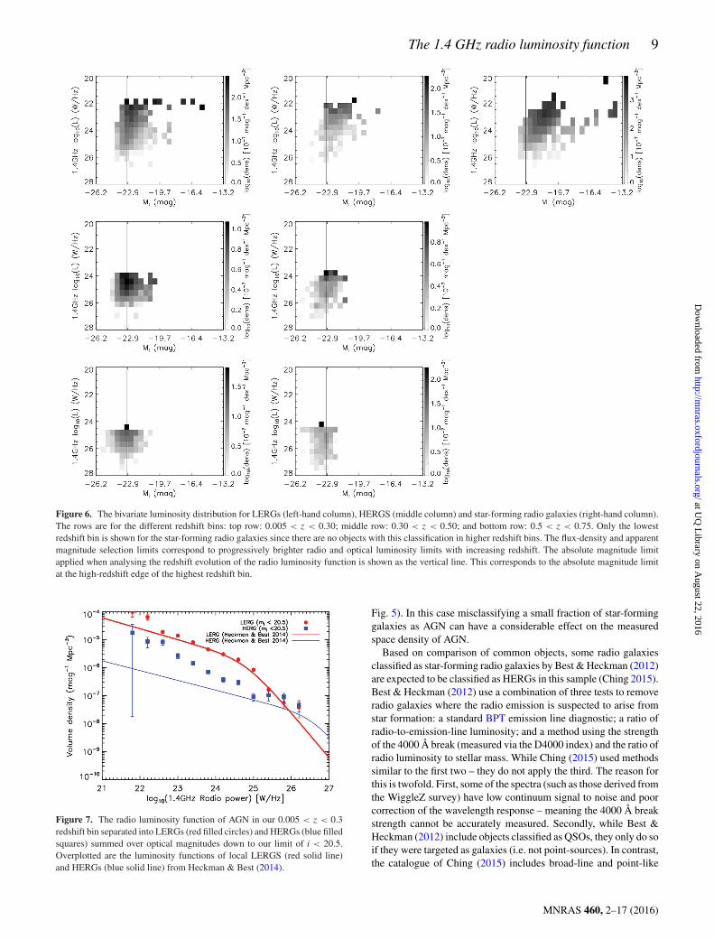
As described in Section 2.1 the AGN in our sample have beenclassified as either LERGs or HERGs based on their optical spectralproperties. In Fig. 6 we show the bivariate luminosity functionfor LERGs (left-hand column), HERGs (middle column) and star-forming radio galaxies (right-hand column) in three redshift bins(top to bottom). The star-forming radio galaxies are shown only forthe low redshift bin, since there are no such objects in the cataloguewith higher redshifts.

In Fig. 7 (and tabulated in Table 2), we show the radio luminos-ity functions for LERGs and HERGs separately, for AGN in our‘local’ 0.005 < z < 0.3 redshift bin. We have summed over opticalluminosities down to the limit of our sample (mi < 20.5). The localLERG and HERG luminosity functions of Best & Heckman (2012,parameters taken from Heckman & Best 2014) are also shown(solid lines). The LERG luminosity functions are similar in shapeand normalization. The HERG luminosity functions, however, aresignificantly different. The HERG luminosity function presentedhere has a higher space density, especially at low radio luminosi-ties. As noted earlier, we do not expect radio luminosity functionsto agree unless they sample the same range of optical luminosities,however, when measured locally this effect should be small andcannot explain the discrepancy.

In the case of the HERGs there are also differences in the clas-sification techniques. Best & Heckman (2012) were deliberatelystrict in removing star-forming radio galaxies. This conservativeapproach is well justified since at the faint end of the radio luminos-ity function the star-forming radio galaxies can dominate in numberdensity over the AGN by approximately an order of magnitude (see

Table 2. The local (0.005 < z < 0.3) 1.4 GHz radio luminosity function from this sample separated into radio AGN and star-forming galaxies. The radioAGN are further separated into LERGs and HERGs.

All galaxies SF galaxies Radio AGN LERGs HERGSlog10P1.4 N log (�) N log (φ) N log (�) N log (�) N log (�)(W Hz−1) (mag−1 Mpc−3) (mag−1 Mpc−3) (mag−1 Mpc−3) (mag−1 Mpc−3) (mag−1 Mpc−3)

21.00 1 −3.58+0.30−3.00 1 −3.58+0.30

−3.00

21.40 14 −3.28+0.10−0.13 14 −3.28+0.10

−0.13

21.80 76 −3.15+0.05−0.05 67 −3.21+0.05

−0.06 9 3.97−+0.12−0.18 8 −4.00+0.13

−0.19 1 −4.75+0.30−3.00

22.20 156 −3.55+0.03−0.04 128 −3.64+0.04

−0.04 28 −4.13+0.08−0.09 22 −4.19+0.08

−0.10 6 −5.06+0.15−0.23

22.60 208 −4.03+0.03−0.03 144 −4.18+0.03

−0.04 64 −4.56+0.05−0.06 46 −4.72+0.06

−0.07 18 −5.07+0.09−0.12

23.0 255 −4.51+0.03−0.03 109 −4.84+0.04

−0.04 146 −4.78+0.03−0.04 124 −4.85+0.04

−0.04 22 −5.58+0.08−0.10

23.40 314 −4.95+0.02−0.03 41 −5.79+0.06

−0.07 273 −5.02+0.03−0.03 234 −5.09+0.03

−0.03 39 −5.84+0.06−0.08

23.80 440 −5.26+0.02−0.02 21 −6.54+0.09

−0.11 419 −5.28+0.02−0.02 368 −5.34+0.02

−0.02 51 −6.15+0.06−0.07

24.20 349 −5.46+0.02−0.02 2 −7.63+0.23

−0.53 347 −5.47+0.02−0.02 319 −5.52+0.02

−0.02 28 −6.43+0.08−0.09

24.60 242 −5.65+0.03−0.03 242 −5.65+0.03

−0.03 217 −5.71+0.03−0.03 25 −6.52+0.08

−0.10

25.00 112 −6.03+0.04−0.04 112 −6.03+0.04

−0.04 101 −6.07+0.04−0.05 11 −7.04+0.11

−0.16

25.40 27 −6.57+0.08−0.09 27 −6.57+0.08

−0.09 20 −6.78+0.09−0.11 7 −6.98+0.14

−0.21

25.80 17 −6.83+0.09−0.12 17 −6.83+0.09

−0.12 7 −7.26+0.14−0.21 10 −7.03+0.12

−0.16

26.20 8 −7.07+0.13−0.19 8 −7.07+0.13

−0.19 3 −7.42+0.20−0.37 5 −7.33+0.16

−0.26

MNRAS 460, 2–17 (2016)

at UQ

Library on A



ownloaded from



Figure 6. The bivariate luminosity distribution for LERGs (left-hand column), HERGS (middle column) and star-forming radio galaxies (right-hand column).The rows are for the different redshift bins: top row: 0.005 < z < 0.30; middle row: 0.30 < z < 0.50; and bottom row: 0.5 < z < 0.75. Only the lowestredshift bin is shown for the star-forming radio galaxies since there are no objects with this classification in higher redshift bins. The flux-density and apparentmagnitude selection limits correspond to progressively brighter radio and optical luminosity limits with increasing redshift. The absolute magnitude limitapplied when analysing the redshift evolution of the radio luminosity function is shown as the vertical line. This corresponds to the absolute magnitude limitat the high-redshift edge of the highest redshift bin.

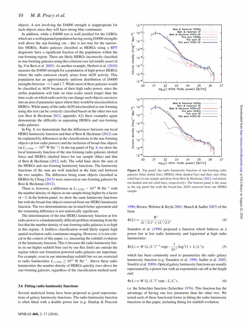
Figure 7. The radio luminosity function of AGN in our 0.005 < z < 0.3redshift bin separated into LERGs (red filled circles) and HERGs (blue filledsquares) summed over optical magnitudes down to our limit of i < 20.5.Overplotted are the luminosity functions of local LERGS (red solid line)and HERGs (blue solid line) from Heckman & Best (2014).

Fig. 5). In this case misclassifying a small fraction of star-forminggalaxies as AGN can have a considerable effect on the measuredspace density of AGN.

Based on comparison of common objects, some radio galaxiesclassified as star-forming radio galaxies by Best & Heckman (2012)are expected to be classified as HERGs in this sample (Ching 2015).Best & Heckman (2012) use a combination of three tests to removeradio galaxies where the radio emission is suspected to arise fromstar formation: a standard BPT emission line diagnostic; a ratio ofradio-to-emission-line luminosity; and a method using the strengthof the 4000 Å break (measured via the D4000 index) and the ratio ofradio luminosity to stellar mass. While Ching (2015) used methodssimilar to the first two – they do not apply the third. The reason forthis is twofold. First, some of the spectra (such as those derived fromthe WiggleZ survey) have low continuum signal to noise and poorcorrection of the wavelength response – meaning the 4000 Å breakstrength cannot be accurately measured. Secondly, while Best &Heckman (2012) include objects classified as QSOs, they only do soif they were targeted as galaxies (i.e. not point-sources). In contrast,the catalogue of Ching (2015) includes broad-line and point-like

MNRAS 460, 2–17 (2016)

at UQ

Library on A



ownloaded from



objects. A test involving the D4000 strength is inappropriate forsuch objects since they will have strong blue continuum.

In addition, while a D4000 test is well justified for the LERGswhich are a wellseparated population having strong D4000 strengthswell above the star-forming cut – this is not true for the narrow-line HERGs. Radio galaxies classified as HERGs using a BPTdiagnostic have a significant fraction of the population within thestar-forming region. These are likely HERGs incorrectly classifiedas star-forming galaxies using this criterion (see left middle panel offig. 9 in Best et al. 2005). As another example, Herbert et al. (2010)measure the D4000 strength for a population of high-power HERGswhere the radio emission clearly arises from AGN activity. Thispopulation has an approximately uniform distribution of D4000strengths between ∼1.1 and 1.7. While most of these galaxies wouldbe classified as AGN because of their high radio power, since thestellar population will fade on time-scales much longer than thetime-scale on which radio activity can change such objects can moveinto an area of parameter space where they would be misclassified asHERGs. While many of the radio AGN misclassified as star-formingusing this test can be correctly classified based on the other two test(see Best & Heckman 2012, appendix A2) these examples againdemonstrate the difficulty in separating HERGs and star-formingradio galaxies.

In Fig. 8, we demonstrate that the differences between our localHERG luminosity function and that of Best & Heckman (2012) canbe explained by differences in the classifications in the star-formingobjects (at low radio powers) and the inclusion of broad-line objects(at L1.4 GHz ∼ 1024 W Hz−1). In the top panel of Fig. 8, we show thelocal luminosity function of the star-forming radio galaxies (dottedlines) and HERGs (dashed lines) for our sample (blue) and thatof Best & Heckman (2012, red). The solid lines show the sum ofthe HERGs and star-forming luminosity functions. The luminosityfunctions of the sum are well matched at the faint end betweenthe two samples. The difference being some objects classified asHERGs by Ching (2015) were removed as star-forming galaxies byBest & Heckman (2012).

There is, however, a difference at L1.4 GHz ∼ 1024 W Hz−1 withthe number density of objects in our sample being higher by a factorof ∼2. In the bottom panel, we show the same luminosity functionsbut with the broad-line objects removed from our HERG luminosityfunction. The two determinations are in much better agreement andthe remaining difference is not statistically significant.

The determination of the true HERG luminosity function at lowradio power is a fundamentally difficult problem stemming from thefact that the number density of star-forming radio galaxies is so highin this regime. A faultless classification would likely require highspatial resolution radio continuum imaging. However, it is not criti-cal in the context of this paper, i.e. measuring the redshift evolutionof the luminosity function. This is because the radio luminosity lim-its in our higher redshift bins (set by our flux limit) are outside theregime where star formation powered radio galaxies are important.For example, even in our intermediate redshift bin we are restrictedto radio luminosities L1.4 GHz � 1024 W Hz−1. Above these radioluminosities the number density of HERGs quickly rises above thestar-forming galaxies, regardless of the classification method used.

3.6 Fitting radio luminosity functions

Several analytical forms have been proposed as good representa-tions of galaxy luminosity functions. The radio luminosity functionis often fitted with a double power law (e.g. Dunlop & Peacock

Figure 8. Top panel: the radio luminosity function of star-forming radiogalaxies (blue dotted line), HERGs (blue dashed line) and their sum (bluesolid line) in our sample and those from Best & Heckman (2012, red dotted,red dashed and red solid lines, respectively). The bottom panel is the sameas the top panel but with the broad-line AGN removed from our HERGsample.

1990; Brown, Webster & Boyle 2001; Mauch & Sadler 2007) of theform

�(L) = �∗

(L∗/L)α + (L∗/L)β. (4)

Saunders et al. (1990) proposed a function which behaves as apower law at low radio luminosity and lognormal at high radioluminosities:

�(L) = �∗(L/L∗)1−α exp(− 1

2σ 2(log2(1 + L/L∗)) (5)

which has been commonly used to parametrize the radio galaxyluminosity function (e.g. Saunders et al. 1990; Sadler et al. 2002;Smolcic et al. 2009). Optical galaxy luminosity functions are usuallyrepresented by a power law with an exponential cut-off at the brightend:

�(L) = �∗(L/L∗)α exp(−L/L∗), (6)

i.e. the Schechter function (Schechter 1976). This function has theadvantage of having one less parameter than the other two. Wetested each of these functional forms in fitting the radio luminosityfunctions in this paper, including fitting for redshift evolution.

MNRAS 460, 2–17 (2016)

at UQ

Library on A



ownloaded from



Figure 9. The radio luminosity function of AGN in our 0.005 < z < 0.3 redshift bin separated into LERGs (red diamonds and solid line) and HERGs (bluetriangles and solid line). Left-hand panel: integrated over i < 20.5 and right-hand panel: galaxies with Mi < −23 only. Overplotted are double power-law fitsto the data (solid lines).

In the case of the HERGs all three functional forms performcomparably with, for example, the difference in Akaike Informa-tion Criterion (AIC; Akaike 1974) in every case being less than 3.An issue which arises in fitting the HERG population is the smallnumber of objects at the bright end where the number density de-creases rapidly. In the case of the double power-law fit (equation 4)this manifests itself as a poor constraint on the bright-end slope β.The sharp drop off in density at high radio luminosities and poorstatistics means that a good fit can be obtained for arbitrarily largenegative β (i.e. as β → −∞ the power-law slope becomes vertical).Similarly, for the fitting function of equation (5) the σ parameteris poorly constrained. The Schechter function fits the data well atthe bright end, although it is not significantly preferred to the othermodels overall.

For the LERGs both equations (4) and (5) allow good analyticalrepresentations of the data, with little difference in the maximumlikelihoods. On the other hand, the Schechter (1976) function isentirely inappropriate (�AIC � 20 in comparison to the other mod-els when fitting for redshift evolution). For our purposes, the mostimportant check is that measuring the rate of redshift evolution (i.e.the KL and KD parameters in equations 7 and 9) is robust. This istrue, since the change in the best-fitting value of these parametersbetween the models is small in comparison to their uncertainties.

In this paper, we have chosen to use the double power-law repre-sentation of equation (4) when fitting the radio luminosity functions.Because of the poor constraints at the bright end of the HERGs, weuse a logarithmic prior on the β parameter. Nevertheless, for theHERGs this parameter essentially only gives an upper limit on thebright-end slope.

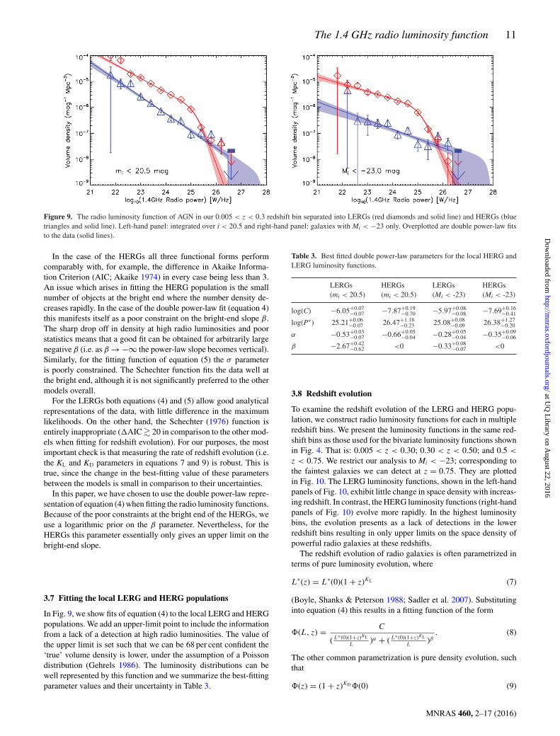
3.7 Fitting the local LERG and HERG populations

In Fig. 9, we show fits of equation (4) to the local LERG and HERGpopulations. We add an upper-limit point to include the informationfrom a lack of a detection at high radio luminosities. The value ofthe upper limit is set such that we can be 68 per cent confident the‘true’ volume density is lower, under the assumption of a Poissondistribution (Gehrels 1986). The luminosity distributions can bewell represented by this function and we summarize the best-fittingparameter values and their uncertainty in Table 3.

Table 3. Best fitted double power-law parameters for the local HERG andLERG luminosity functions.

LERGs HERGs LERGs HERGs(mi < 20.5) (mi < 20.5) (Mi < -23) (Mi < -23)

log(C) −6.05+0.07−0.07 −7.87+0.19

−0.70 −5.97+0.08−0.08 −7.69+0.16

−0.41

log(P∗) 25.21+0.06−0.07 26.47+1.18

−0.23 25.08+0.08−0.09 26.38+1.27

−0.20

α −0.53+0.03−0.07 −0.66+0.05

−0.04 −0.28+0.05−0.04 −0.35+0.09

−0.06

β −2.67+0.42−0.62 <0 −0.33+0.08

−0.07 <0

3.8 Redshift evolution

To examine the redshift evolution of the LERG and HERG popu-lation, we construct radio luminosity functions for each in multipleredshift bins. We present the luminosity functions in the same red-shift bins as those used for the bivariate luminosity functions shownin Fig. 4. That is: 0.005 < z < 0.30; 0.30 < z < 0.50; and 0.5 <

z < 0.75. We restrict our analysis to Mi < −23; corresponding tothe faintest galaxies we can detect at z = 0.75. They are plottedin Fig. 10. The LERG luminosity functions, shown in the left-handpanels of Fig. 10, exhibit little change in space density with increas-ing redshift. In contrast, the HERG luminosity functions (right-handpanels of Fig. 10) evolve more rapidly. In the highest luminositybins, the evolution presents as a lack of detections in the lowerredshift bins resulting in only upper limits on the space density ofpowerful radio galaxies at these redshifts.

The redshift evolution of radio galaxies is often parametrized interms of pure luminosity evolution, where

L∗(z) = L∗(0)(1 + z)KL (7)

(Boyle, Shanks & Peterson 1988; Sadler et al. 2007). Substitutinginto equation (4) this results in a fitting function of the form

�(L, z) = C

( L∗(0)(1+z)KL

L)α + ( L∗(0)(1+z)KL

L)β

. (8)

The other common parametrization is pure density evolution, suchthat

�(z) = (1 + z)KD�(0) (9)

MNRAS 460, 2–17 (2016)

at UQ

Library on A



ownloaded from



Figure 10. The radio luminosity function for LERGs (left-hand column) and HERGs (right-hand column) separated into three redshift bins: 0.005 < z < 0.30(blue); 0.30 < z < 0.50 (green); 0.5 < z < 0.75 (red). The top row shows the fit to the data (solid lines) assuming pure density evolution and the bottom rowshows the fit to the data assuming pure luminosity evolution.

giving

�(L, z) = C(1 + z)KD

(L∗/L)α + (L∗/L)β. (10)

There is a degeneracy between luminosity and density evolution,especially when the bright population is not tightly constrained (LeFloc’h et al. 2005; Smolcic et al. 2009). We therefore do not fitjointly for luminosity and density evolution but restrict ourselves tothe cases above.

We fitted, using a Markov Chain Monte Carlo (MCMC) method,both the LERGs (left-hand column of Fig. 10) and HERGs (right-hand column of Fig. 10) with a pure density evolution model (toprow of Fig. 10) and a pure luminosity evolution model (second row ofFig. 10). The evolution in the LERGs can be well represented by ei-ther model with the pure luminosity evolution marginally preferredwith difference in AIC of ∼ 3.5 (equivalent to a maximum likelihoodratio of ∼6). In the case of the HERGs, there is a similar prefer-ence for the pure density evolution model with a difference in AIC∼ 3.1 equivalent to a maximum likelihood ratio of ∼4.5. The best-fitting parameters and their uncertainties are summarized in Table 4.Parametrized in this way, the LERGs evolve slowly with redshift as

∼(1 + z)0.06+0.17−0.18 assuming pure density evolution or ∼(1 + z)0.46+0.22

−0.24

assuming pure luminosity evolution. Under both assumptions this isconsistent with no evolution within ∼2σ . The HERGs evolve faster

Table 4. Best fitted double power-law parameters for the redshift evolutionof the LERGs and HERGs.

LERGs HERGsDensity Luminosity Density Luminosity

log(C) −6.05+0.07−0.06 −6.06+0.06

−0.05 −8.04+0.17−0.24 −7.59+0.12

−0.19

log(P∗) 25.17+0.06−0.06 25.12+0.06

−0.07 26.96+0.27−0.19 25.66+0.40

−0.23

α −0.31+0.04−0.03 −0.32+0.04

−0.03 −0.32+0.04−0.05 0.35+0.04

−0.05

β −1.88+0.10−0.12 −1.92+0.12

−0.11 −1.75+0.29−1.40 −2.17+0.49

−4.50

KD,L 0.06+0.17−0.18 0.46+0.22

−0.24 2.93+0.46−047 7.41+0.79

−1.33

than the LERGs with ∼(1 + z)2.93+0.46−0.47 in the pure density evolution

case. If a pure luminosity evolution model is used, the parametrized

redshift dependence is very rapid ∼(1 + z)7.41+0.79−1.33 . The luminosity

functions for the LERGs and the HERGs are tabulated in Tables 5and 6.

4 D I SCUSSI ON

It is well established that there is luminosity-dependent evolutionin the overall radio AGN population, in the sense that the spacedensity of the high luminosity population increases more rapidlywith redshift (e.g. Longair 1966; Doroshkevich et al. 1970; Willott

MNRAS 460, 2–17 (2016)

at UQ

Library on A



ownloaded from



Table 5. Luminosity function of LERGs in three redshift bins (0.005 < z <

0.30, 0.30 < z < 0.50, 0.50 < z < 0.75). Only galaxies with optical I-bandabsolute magnitude Mi < −23 are included.

0.005 < z < 0.30 0.30 < z < 0.50 0.50 < z < 0.75log10P1.4 N log (�) N log (�) N log (�)(W Hz−1) (mag−1 Mpc−3) (mag−1 Mpc−3) (mag−1 Mpc−3)

21.80 1 −4.78+0.30−3.00

22.20 4 −5.13+0.18−0.30

22.60 15 −5.16+0.10−0.13

23.00 34 −5.42+0.07−0.08

23.40 96 −5.49+0.04−0.05

23.80 216 −5.61+0.03−0.03 8 −5.82+0.13

−0.19

24.20 193 −5.77+0.03−0.03 289 −5.75+0.02

−0.03 1 −5.11+0.30−3.00

24.60 163 −5.85+0.03−0.04 371 −5.91+0.02

−0.02 213 −5.93+0.03−0.03

25.00 79 −6.19+0.05−0.05 218 −6.15+0.03

−0.03 242 −6.21+0.03−0.03

25.40 17 −6.84+0.09−0.12 77 −6.64+0.05

−0.05 121 −6.53+0.04−0.04

25.80 7 −7.23+0.14−0.21 17 −7.27+0.09

−0.12 45 −7.01+0.06−0.07

26.20 1 −8.07+0.30−3.00 1 −8.57+0.30

−3.00 11 −7.55+0.11−0.16

26.60 1 −8.36+0.30−3.00 2 −8.24+0.23

−0.53

27.00 1 −8.60+0.30−3.00 1 −8.62+0.30

−2.98

27.40 1 −8.35+0.30−3.00

Table 6. Luminosity function of HERGs in three redshift bins (0.005 <

z < 0.30, 0.30 < z < 0.50, 0.50 < z < 0.75). Only galaxies with opticalI-band absolute magnitude Mi < −23 are included.

0.005 < z < 0.30 0.30 < z < 0.50 0.50 < z < 0.75log10P1.4 N log (�) N log (�) N log (�)(W Hz−1) (mag−1 Mpc−3) (mag−1 Mpc−3) (mag−1 Mpc−3)

22.20 1 −5.34+0.30−3.00

22.60 1 −6.53+0.30−3.00

23.00 2 −6.54+0.23−0.53

23.40 7 −6.60+0.14−0.21

23.80 18 −6.60+0.09−0.12 3 −5.93+0.20

−0.37

24.20 8 −7.04+0.13−0.19 28 −6.46+0.08

−0.09 1 −4.76+0.30−3.00

24.60 12 −6.89+0.11−0.15 25 −7.00+0.08

−0.10 47 −6.72+0.06−0.07

25.00 5 −7.41+0.16−0.26 19 −7.05+0.09

−0.11 46 −6.74+0.06−0.07

25.40 2 −7.48+0.23−0.53 26 −6.99+0.08

−0.09 42 −6.83+0.06−0.07

25.80 8 −7.10+0.13−0.19 10 −7.38+0.12

−0.16 35 −7.06+7.06−0.08

26.20 4 −7.36+0.18−0.30 16 −7.23+0.10

−0.12 30 −7.17+0.07−0.09

26.60 4 7.80−+0.18−0.30 16 −7.43+0.10

−0.12

27.00 3 −7.89+0.20−0.37 7 −7.75+0.14

−0.21

27.40 4 −8.10+0.18−0.30

27.80 1 −8.98+0.30−3.02

et al. 2001; Sadler et al. 2007; Smolcic et al. 2009). This differen-tial evolution can be explained by a two-population scenario wherethe LERGs dominate the space density at all but the highest ra-dio luminosity and evolve slowly with redshift, while the HERGsthat dominate at the highest radio luminosities evolve more rapidly(Smolcic et al. 2009; Best & Heckman 2012; Best et al. 2014).

The expectation is that the LERGs are hosted by quiescent galax-ies and powered by Bondi & Hoyle (1944) accretion from theirhot gas atmospheres (e.g. Hardcastle et al. 2007; Best & Heckman2012). In this case, a first-order prediction is that the LERGs will

evolve in a similar manner to the stellar mass function of massivequiescent galaxies. In this case, a mild decrease with increasingredshift is expected over the redshift range considered here (i.e.z < 0.75) evolving down in space density as ∼(1 + z)−0.1 (Best et al.2014). In reality, the evolution will be complicated by dependenceon quantities like the halo hot gas fraction and the cooling function(e.g. Croton et al. 2006) and the average density of the mediuminto which the radio jets are expanding (Best et al. 2014). Crotonet al. (2006) predict an almost flat black hole accretion rate densityover this redshift range (see Fig. 13). In any case, the expectationis we should observe little evolution in our LERG luminosity func-tion out to z = 0.75, and this is the case with our best-fitting pure

density evolution model evolving as ∼(1 + z)0.06+0.17−0.18 consistent with

zero evolution. It should be noted that the evolution measured fromour luminosity functions is only for the optically brightest galaxies(Mi < −23.0), and that our application of an e-correction meanswe are including the same stellar mass hosts at all redshifts. Ifthe e-correction is not applied our luminosity functions would dis-play a significant positive redshift evolution of the space density of

∼(1 + z)0.81+0.15−0.16 (assuming pure density evolution).

In this duel accretion mode picture, the HERGs are some subsetof the optical quasars and Seyfert galaxies. Croom et al. (2009)measured the evolution of the QSO luminosity function in the inter-val 0.4 < z < 2.6 using the 2SLAQ sample. At the lowest redshifts(z � 1), the number density evolves rapidly in a manner that de-pends on luminosity – in the sense that the brightest QSOs evolvefaster. At the bright end (Mg ∼ −24), the space density increasesbetween their lowest redshift bins (0.40 < z < 0.68 and 0.68 < z

< 1.06) by a factor of ∼3 which is similar to the change expectedfrom our best-fitting pure density model which has space densityevolving as ∼(1 + z)2.93.

We did not apply an e-correction for the HERGs when construct-ing the bivariate luminosity functions. Since the HERGs often haveongoing star formation and it is plausible that the AGN activity andstar formation histories are related – it is inappropriate to representthem as having a stellar population which fades with time as it ages.Generally the recent star formation will contribute much of the op-tical light, nevertheless there will be some fading of the underlyingolder stellar population. Applying an e-correction will reduce themagnitude of the evolution in the luminosity function since it shiftshigher redshift objects fainter and out of the selection limits. To in-vestigate the maximum difference an e-correction could make to theevolution of the HERG luminosity function, we applied the samee-correction for the HERGs as was applied to the LERGs (whichwill overestimate the magnitude of the correction) and fitted for theevolution. In the pure density evolution case, we find evolution in

the space density of ∼(1 + z)2.14+0.52−0.63 . If a pure luminosity evolution

model is used, the redshift dependence is ∼(1 + z)5.78+0.92−2.01 .

A clear difference between the luminosity functions of the LERGsand the HERGs is the radio power of the turnover. The bright-endturn down in the HERG luminosity function is ∼1 dex brighter thanthat of the LERGs (see e.g. Fig. 10 or Table 4). The bright-endcut-off in the i-band optical luminosity function of our HERGs andLERGs is approximately the same (see abscissa values of Fig. 6);implying, to first order, a similar cut-off in the black hole massfunction of the two samples. The origin of the high power cut-offin the radio luminosity function is likely related to the cut-off in theblack hole mass function modulated in some way by the accretionrate and jet-production efficiency. The Eddington scaled accretionrate in the HERGs is expected to be 1–2 dex higher than in LERGs(Best & Heckman 2012; Mingo et al. 2014; Fernandes et al. 2015;

MNRAS 460, 2–17 (2016)

at UQ

Library on A



ownloaded from



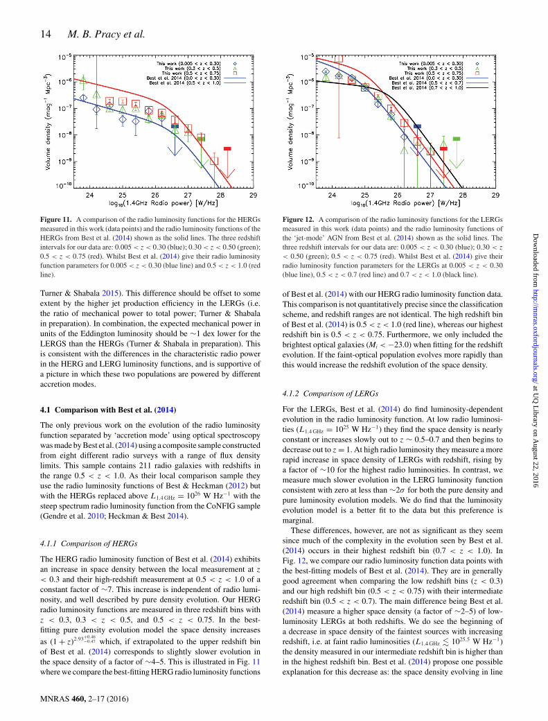
Figure 11. A comparison of the radio luminosity functions for the HERGsmeasured in this work (data points) and the radio luminosity functions of theHERGs from Best et al. (2014) shown as the solid lines. The three redshiftintervals for our data are: 0.005 < z < 0.30 (blue); 0.30 < z < 0.50 (green);0.5 < z < 0.75 (red). Whilst Best et al. (2014) give their radio luminosityfunction parameters for 0.005 < z < 0.30 (blue line) and 0.5 < z < 1.0 (redline).

Turner & Shabala 2015). This difference should be offset to someextent by the higher jet production efficiency in the LERGs (i.e.the ratio of mechanical power to total power; Turner & Shabalain preparation). In combination, the expected mechanical power inunits of the Eddington luminosity should be ∼1 dex lower for theLERGS than the HERGs (Turner & Shabala in preparation). Thisis consistent with the differences in the characteristic radio powerin the HERG and LERG luminosity functions, and is supportive ofa picture in which these two populations are powered by differentaccretion modes.

4.1 Comparison with Best et al. (2014)

The only previous work on the evolution of the radio luminosityfunction separated by ‘accretion mode’ using optical spectroscopywas made by Best et al. (2014) using a composite sample constructedfrom eight different radio surveys with a range of flux densitylimits. This sample contains 211 radio galaxies with redshifts inthe range 0.5 < z < 1.0. As their local comparison sample theyuse the radio luminosity functions of Best & Heckman (2012) butwith the HERGs replaced above L1.4 GHz = 1026 W Hz−1 with thesteep spectrum radio luminosity function from the CoNFIG sample(Gendre et al. 2010; Heckman & Best 2014).

4.1.1 Comparison of HERGs

The HERG radio luminosity function of Best et al. (2014) exhibitsan increase in space density between the local measurement at z

< 0.3 and their high-redshift measurement at 0.5 < z < 1.0 of aconstant factor of ∼7. This increase is independent of radio lumi-nosity, and well described by pure density evolution. Our HERGradio luminosity functions are measured in three redshift bins withz < 0.3, 0.3 < z < 0.5, and 0.5 < z < 0.75. In the best-fitting pure density evolution model the space density increases

as (1 + z)2.93+0.46−0.47 which, if extrapolated to the upper redshift bin

of Best et al. (2014) corresponds to slightly slower evolution inthe space density of a factor of ∼4–5. This is illustrated in Fig. 11where we compare the best-fitting HERG radio luminosity functions

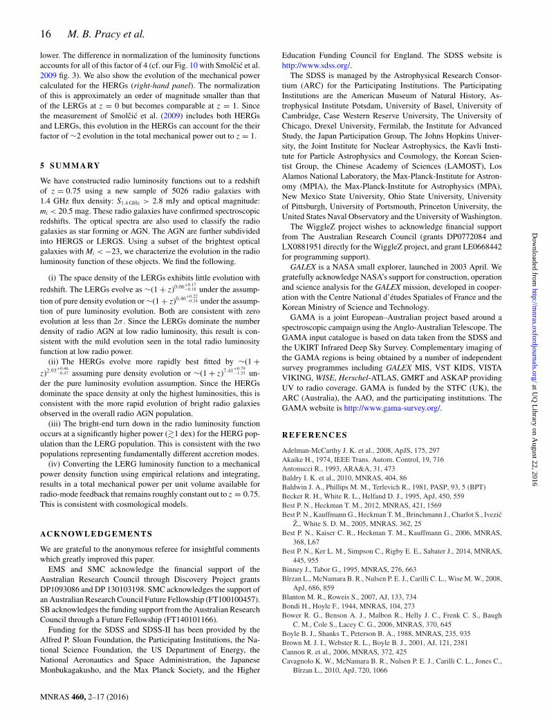
Figure 12. A comparison of the radio luminosity functions for the LERGsmeasured in this work (data points) and the radio luminosity functions ofthe ‘jet-mode’ AGN from Best et al. (2014) shown as the solid lines. Thethree redshift intervals for our data are: 0.005 < z < 0.30 (blue); 0.30 < z

< 0.50 (green); 0.5 < z < 0.75 (red). Whilst Best et al. (2014) give theirradio luminosity function parameters for the LERGs at 0.005 < z < 0.30(blue line), 0.5 < z < 0.7 (red line) and 0.7 < z < 1.0 (black line).

of Best et al. (2014) with our HERG radio luminosity function data.This comparison is not quantitatively precise since the classificationscheme, and redshift ranges are not identical. The high redshift binof Best et al. (2014) is 0.5 < z < 1.0 (red line), whereas our highestredshift bin is 0.5 < z < 0.75. Furthermore, we only included thebrightest optical galaxies (Mi < −23.0) when fitting for the redshiftevolution. If the faint-optical population evolves more rapidly thanthis would increase the redshift evolution of the space density.

4.1.2 Comparison of LERGs

For the LERGs, Best et al. (2014) do find luminosity-dependentevolution in the radio luminosity function. At low radio luminosi-ties (L1.4 GHz = 1025 W Hz−1) they find the space density is nearlyconstant or increases slowly out to z ∼ 0.5–0.7 and then begins todecrease out to z = 1. At high radio luminosity they measure a morerapid increase in space density of LERGs with redshift, rising bya factor of ∼10 for the highest radio luminosities. In contrast, wemeasure much slower evolution in the LERG luminosity functionconsistent with zero at less than ∼2σ for both the pure density andpure luminosity evolution models. We do find that the luminosityevolution model is a better fit to the data but this preference ismarginal.

These differences, however, are not as significant as they seemsince much of the complexity in the evolution seen by Best et al.(2014) occurs in their highest redshift bin (0.7 < z < 1.0). InFig. 12, we compare our radio luminosity function data points withthe best-fitting models of Best et al. (2014). They are in generallygood agreement when comparing the low redshift bins (z < 0.3)and our high redshift bin (0.5 < z < 0.75) with their intermediateredshift bin (0.5 < z < 0.7). The main difference being Best et al.(2014) measure a higher space density (a factor of ∼2–5) of low-luminosity LERGs at both redshifts. We do see the beginning ofa decrease in space density of the faintest sources with increasingredshift, i.e. at faint radio luminosities (L1.4 GHz � 1025.5 W Hz−1)the density measured in our intermediate redshift bin is higher thanin the highest redshift bin. Best et al. (2014) propose one possibleexplanation for this decrease as: the space density evolving in line

MNRAS 460, 2–17 (2016)

at UQ

Library on A



ownloaded from



with the density of massive quiescent galaxies and a time delaybetween the onset of the radio AGN after the formation of thequiescent host galaxy.

As pointed out earlier, when considering redshift evolution, sam-ples with the same optical brightness constraints should be usedotherwise different fractions of the total population will be countedat different redshifts. Best et al. (2014) do not apply such a con-straint instead mitigating such effects by only including surveyswith high redshift completeness in their sample. For example, at acompleteness of unity all radio sources are counted and there willbe no optical selection effects. Best et al. (2014) do not state theirspectroscopic completeness values for all eight of the radio surveysused in their combined sample, however, in several cases they re-strict their flux density ranges to ensure completeness. We, however,only include the optically brightest galaxies in our sample (Mi <

−23) which has the effect of decreasing the normalization of theluminosity function. We have already demonstrated that when wedo not restrict our sample to Mi < −23 our local LERG luminosityfunction agrees with that of Best et al. (2014, see Fig. 5).

4.2 Radio-mode feedback

There is substantial evidence that radio jets from LERGs are im-portant in regulating star formation in massive galaxies and clustersof galaxies by injecting energy into the hot gas atmosphere andinhibiting gas cooling and star formation. This radio-mode AGNfeedback can simultaneously explain the ‘cooling flow problem’,the exponential cut-off in the bright end of the optical galaxy lumi-nosity function and the old stellar populations of the most massivebulges (e.g. Bower et al. 2006; Croton et al. 2006). Estimates ofthe energy associated with bubbles and cavities in the intergalacticmedium surrounding elliptical galaxies and galaxy clusters can beused to estimate the mechanical power associated with the radio jetsproducing the cavities. The empirical correlation of these energieswith monochromatic radio luminosity can be used to transform be-tween the two (Dunn, Fabian & Taylor 2005; Rafferty et al. 2006;Bırzan et al. 2008; Cavagnolo et al. 2010). Although, these relationshave large intrinsic scatter of ∼0.7 dex (Cavagnolo et al. 2010).Using such relations the monochromatic radio luminosity function

can be transformed into a mechanical power density function, andintegrated to calculate the total mechanical power (per unit volume)available for radio-mode feedback (e.g. Best et al. 2006; Smolcicet al. 2009). That is, we calculate

∫φ(Pm) Pm d(0.4 log10 Pm) = 2.5

ln(10)

∫φ(Pm) dPm (11)

where Pm is the mechanical power which we calculate from the1.4 GHz luminosity using equation 1 of Cavagnolo et al. (2010).The factor of 2.5/ln (10) comes about since our luminosity functionis in units of mag−1 rather than units of the natural logarithm.

In Fig. 13, we show this integral as a function of redshift usingour pure density evolution fits to the LERGs and HERGs. We fol-low Smolcic et al. (2009) and integrate above a mechanical powerequivalent to L1.4GHz = 1021 W Hz−1. The shaded regions illustratethe uncertainties from the conversion of 1.4 GHz radio luminosityto mechanical power using the uncertainties quoted in Cavagnoloet al. (2010, equation 1) (large shaded regions), and from the un-certainties in our parameter values from fitting the radio luminosityfunction; constructed by sampling the posterior distribution of theparameters obtained from the MCMC fitting (smaller dark shadedregions).

There is little evolution with redshift in the volume density ofmechanical power from the LERGs (left-hand panel of Fig. 13),consistent with the prediction from the cosmological model of Cro-ton et al. (2006); shown as the dashed line. It should be noted thesemechanical powers only include emission from massive galaxiessince our radio luminosity functions are restricted to Mi < −23,including fainter optical galaxies will increase the normalizationfurther. Also, in the left-hand panel of Fig. 13 we show the me-chanical power calculated from fits to the radio luminosity func-tion of low-luminosity VLA-COSMOS AGN (Smolcic et al. 2009).The low-luminosity selection means the radio luminosity functionshould be dominated by LERGs although it will still contain a con-tribution from the HERGs. The normalization of our estimate ofthe total mechanical power is a factor of ∼4 lower than that mea-sured by Smolcic et al. (2009). This difference can be attributedto our restriction to only the very brightest optical galaxies (Mi <

−23) causing the normalization of our luminosity functions to be

Figure 13. The total mechanical power per unit volume as function of redshift estimated from the pure density evolution fits to our radio luminosity functions.The conversion to mechanical power from 1.4 GHz luminosity uses the relation of Cavagnolo et al. (2010). The shaded regions represent the uncertainty fromthe radio luminosity function fits (smaller dark shaded regions) and the uncertainty in the Cavagnolo et al. (2010) relation (the larger shaded regions). Theleft-hand panel is for the LERGs and the right-hand panel is for the HERGs. Also overplotted on the LERGs are the prediction from the cosmological modelof Croton et al. (2006) and the measurement from Smolcic et al. (2009).The difference in normalization between our measurement and that of Smolcic et al.(2009) can be entirely attributed to our measurement only including the contribution from the brightest optical galaxies (see text for details).

MNRAS 460, 2–17 (2016)

at UQ

Library on A



ownloaded from



lower. The difference in normalization of the luminosity functionsaccounts for all of this factor of 4 (cf. our Fig. 10 with Smolcic et al.2009 fig. 3). We also show the evolution of the mechanical powercalculated for the HERGs (right-hand panel). The normalizationof this is approximately an order of magnitude smaller than thatof the LERGs at z = 0 but becomes comparable at z = 1. Sincethe measurement of Smolcic et al. (2009) includes both HERGsand LERGs, this evolution in the HERGs can account for the theirfactor of ∼2 evolution in the total mechanical power out to z = 1.

5 SU M M A RY

We have constructed radio luminosity functions out to a redshiftof z = 0.75 using a new sample of 5026 radio galaxies with1.4 GHz flux density: S1.4 GHz > 2.8 mJy and optical magnitude:mi < 20.5 mag. These radio galaxies have confirmed spectroscopicredshifts. The optical spectra are also used to classify the radiogalaxies as star forming or AGN. The AGN are further subdividedinto HERGS or LERGS. Using a subset of the brightest opticalgalaxies with Mi < −23, we characterize the evolution in the radioluminosity function of these objects. We find the following.

(i) The space density of the LERGs exhibits little evolution with

redshift. The LERGs evolve as ∼(1 + z)0.06+0.17−0.18 under the assump-

tion of pure density evolution or ∼(1 + z)0.46+0.22−0.24 under the assump-

tion of pure luminosity evolution. Both are consistent with zeroevolution at less than 2σ . Since the LERGs dominate the numberdensity of radio AGN at low radio luminosity, this result is con-sistent with the mild evolution seen in the total radio luminosityfunction at low radio power.

(ii) The HERGs evolve more rapidly best fitted by ∼(1 +z)2.93+0.46

−0.47 assuming pure density evolution or ∼(1 + z)7.41+0.79−1.33 un-

der the pure luminosity evolution assumption. Since the HERGsdominate the space density at only the highest luminosities, this isconsistent with the more rapid evolution of bright radio galaxiesobserved in the overall radio AGN population.

(iii) The bright-end turn down in the radio luminosity functionoccurs at a significantly higher power (�1 dex) for the HERG pop-ulation than the LERG population. This is consistent with the twopopulations representing fundamentally different accretion modes.

(iv) Converting the LERG luminosity function to a mechanicalpower density function using empirical relations and integrating,results in a total mechanical power per unit volume available forradio-mode feedback that remains roughly constant out to z = 0.75.This is consistent with cosmological models.

AC K N OW L E D G E M E N T S

We are grateful to the anonymous referee for insightful commentswhich greatly improved this paper.

EMS and SMC acknowledge the financial support of theAustralian Research Council through Discovery Project grantsDP1093086 and DP 130103198. SMC acknowledges the support ofan Australian Research Council Future Fellowship (FT100100457).SB acknowledges the funding support from the Australian ResearchCouncil through a Future Fellowship (FT140101166).

Funding for the SDSS and SDSS-II has been provided by theAlfred P. Sloan Foundation, the Participating Institutions, the Na-tional Science Foundation, the US Department of Energy, theNational Aeronautics and Space Administration, the JapaneseMonbukagakusho, and the Max Planck Society, and the Higher

Education Funding Council for England. The SDSS website ishttp://www.sdss.org/.

The SDSS is managed by the Astrophysical Research Consor-tium (ARC) for the Participating Institutions. The ParticipatingInstitutions are the American Museum of Natural History, As-trophysical Institute Potsdam, University of Basel, University ofCambridge, Case Western Reserve University, The University ofChicago, Drexel University, Fermilab, the Institute for AdvancedStudy, the Japan Participation Group, The Johns Hopkins Univer-sity, the Joint Institute for Nuclear Astrophysics, the Kavli Insti-tute for Particle Astrophysics and Cosmology, the Korean Scien-tist Group, the Chinese Academy of Sciences (LAMOST), LosAlamos National Laboratory, the Max-Planck-Institute for Astron-omy (MPIA), the Max-Planck-Institute for Astrophysics (MPA),New Mexico State University, Ohio State University, Universityof Pittsburgh, University of Portsmouth, Princeton University, theUnited States Naval Observatory and the University of Washington.

The WiggleZ project wishes to acknowledge financial supportfrom The Australian Research Council (grants DP0772084 andLX0881951 directly for the WiggleZ project, and grant LE0668442for programming support).

GALEX is a NASA small explorer, launched in 2003 April. Wegratefully acknowledge NASA’s support for construction, operationand science analysis for the GALEX mission, developed in cooper-ation with the Centre National d’etudes Spatiales of France and theKorean Ministry of Science and Technology.

GAMA is a joint European–Australian project based around aspectroscopic campaign using the Anglo-Australian Telescope. TheGAMA input catalogue is based on data taken from the SDSS andthe UKIRT Infrared Deep Sky Survey. Complementary imaging ofthe GAMA regions is being obtained by a number of independentsurvey programmes including GALEX MIS, VST KIDS, VISTAVIKING, WISE, Herschel-ATLAS, GMRT and ASKAP providingUV to radio coverage. GAMA is funded by the STFC (UK), theARC (Australia), the AAO, and the participating institutions. TheGAMA website is http://www.gama-survey.org/.

R E F E R E N C E S

Adelman-McCarthy J. K. et al., 2008, ApJS, 175, 297Akaike H., 1974, IEEE Trans. Autom. Control, 19, 716Antonucci R., 1993, ARA&A, 31, 473Baldry I. K. et al., 2010, MNRAS, 404, 86Baldwin J. A., Phillips M. M., Terlevich R., 1981, PASP, 93, 5 (BPT)Becker R. H., White R. L., Helfand D. J., 1995, ApJ, 450, 559Best P. N., Heckman T. M., 2012, MNRAS, 421, 1569Best P. N., Kauffmann G., Heckman T. M., Brinchmann J., Charlot S., Ivezic

Z., White S. D. M., 2005, MNRAS, 362, 25Best P. N., Kaiser C. R., Heckman T. M., Kauffmann G., 2006, MNRAS,

368, L67Best P. N., Ker L. M., Simpson C., Rigby E. E., Sabater J., 2014, MNRAS,

445, 955Binney J., Tabor G., 1995, MNRAS, 276, 663Bırzan L., McNamara B. R., Nulsen P. E. J., Carilli C. L., Wise M. W., 2008,

ApJ, 686, 859Blanton M. R., Roweis S., 2007, AJ, 133, 734Bondi H., Hoyle F., 1944, MNRAS, 104, 273Bower R. G., Benson A. J., Malbon R., Helly J. C., Frenk C. S., Baugh

C. M., Cole S., Lacey C. G., 2006, MNRAS, 370, 645Boyle B. J., Shanks T., Peterson B. A., 1988, MNRAS, 235, 935Brown M. J. I., Webster R. L., Boyle B. J., 2001, AJ, 121, 2381Cannon R. et al., 2006, MNRAS, 372, 425Cavagnolo K. W., McNamara B. R., Nulsen P. E. J., Carilli C. L., Jones C.,

Bırzan L., 2010, ApJ, 720, 1066

MNRAS 460, 2–17 (2016)

at UQ

Library on A



ownloaded from

http://www.sdss.org/

http://www.gama-survey.org/



Chiaberge M., Macchetto F. D., Sparks W. B., Capetti A., Allen M. G.,Martel A. R., 2002, ApJ, 571, 247

Ching J., 2015, PhD thesis, Sydney Univ.Cirasuolo M., Magliocchetti M., Gentile G., Celotti A., Cristiani S., Danese

L., 2006, MNRAS, 371, 695Clewley L., Jarvis M. J., 2004, MNRAS, 352, 909Condon J. J., Cotton W. D., Greisen E. W., Yin Q. F., Perley R. A., Taylor

G. B., Broderick J. J., 1998, AJ, 115, 1693Condon J. J., Cotton W. D., Broderick J. J., 2002, AJ, 124, 675Croom S. M., Smith R. J., Boyle B. J., Shanks T., Miller L., Outram P. J.,

Loaring N. S., 2004, MNRAS, 349, 1397Croom S. M. et al., 2009, MNRAS, 392, 19Croton D. J. et al., 2006, MNRAS, 365, 11Davis T. A. et al., 2012, MNRAS, 426, 1574Donoso E., Best P. N., Kauffmann G., 2009, MNRAS, 392, 617Doroshkevich A. G., Longair M. S., Zeldovich Y. B., 1970, MNRAS, 147,

139Drinkwater M. J. et al., 2010, MNRAS, 401, 1429Driver S. P. et al., 2011, MNRAS, 413, 971Dunlop J. S., Peacock J. A., 1990, MNRAS, 247, 19Dunn R. J. H., Fabian A. C., Taylor G. B., 2005, MNRAS, 364, 1343Fabian A. C., Celotti A., Blundell K. M., Kassim N. E., Perley R. A., 2002,

MNRAS, 331, 369Fernandes C. A. C. et al., 2015, MNRAS, 447, 1184Ganguly R., Brotherton M. S., 2008, ApJ, 672, 102Gebhardt K. et al., 2000, ApJ, 539, L13Gehrels N., 1986, ApJ, 303, 336Gendre M. A., Best P. N., Wall J. V., 2010, MNRAS, 404, 1719Hardcastle M. J., Evans D. A., Croston J. H., 2007, MNRAS, 376, 1849Harrison C. M., Alexander D. M., Mullaney J. R., Swinbank A. M., 2014,

MNRAS, 441, 3306Heckman T. M., Best P. N., 2014, ARA&A, 52, 589Herbert P. D., Jarvis M. J., Willott C. J., McLure R. J., Mitchell E., Rawlings

S., Hill G. J., Dunlop J. S., 2010, MNRAS, 406, 1841Hill G. J., Rawlings S., 2003, New Astron. Rev., 47, 373Hine R. G., Longair M. S., 1979, MNRAS, 188, 111Ivezic Z. et al., 2002, AJ, 124, 2364Jackson N., Rawlings S., 1997, MNRAS, 286, 241Jackson C. A., Wall J. V., 1999, MNRAS, 304, 160Kauffmann G. et al., 2003, MNRAS, 346, 1055Kauffmann G., Heckman T. M., Best P. N., 2008, MNRAS, 384, 953Lacy M., Rawlings S., Hill G. J., Bunker A. J., Ridgway S. E., Stern D.,

1999, MNRAS, 308, 1096Laing R. A., Jenkins C. R., Wall J. V., Unger S. W., 1994, in Bicknell G. V.,

Dopita M. A., Quinn P. J., eds, ASP Conf. Ser. Vol. 54, The Physics ofActive Galaxies. Astron. Soc. Pac., San Francisco, p. 201

Le Floc’h E., Papovich C., Dole H., Bell E. F., Lagache G., 2005, ApJ, 632,169

Liske J. et al., 2015, MNRAS, 452, 2087Longair M. S., 1966, MNRAS, 133, 421McAlpine K., Jarvis M. J., Bonfield D. G., 2013, MNRAS, 436, 1084McElroy R., Croom S. M., Pracy M., Sharp R., Ho I.-T., Medling A. M.,

2015, MNRAS, 446, 2186Machalski J., Godlowski W., 2000, A&A, 360, 463McNamara B. R., Nulsen P. E. J., 2007, ARA&A, 45, 117Magorrian J. et al., 1998, AJ, 115, 2285Mao M. Y. et al., 2012, MNRAS, 426, 3334Mauch T., Sadler E. M., 2007, MNRAS, 375, 931Mingo B., Hardcastle M. J., Croston J. H., Dicken D., Evans D. A., Morganti

R., Tadhunter C., 2014, MNRAS, 440, 269Page M. J. et al., 2012, Nature, 485, 213Peacock J. A., 1985, MNRAS, 217, 601Poggianti B. M., 1997, A&AS, 122, 399Rafferty D. A., McNamara B. R., Nulsen P. E. J., Wise M. W., 2006, ApJ,

652, 216Rigby E. E., Best P. N., Brookes M. H., Peacock J. A., Dunlop J. S.,

Rottgering H. J. A., Wall J. V., Ker L., 2011, MNRAS, 416, 1900Sadler E. M. et al., 2002, MNRAS, 329, 227Sadler E. M. et al., 2007, MNRAS, 381, 211Saunders W., Rowan-Robinson M., Lawrence A., Efstathiou G., Kaiser N.,

Ellis R. S., Frenk C. S., 1990, MNRAS, 242, 318Schechter P., 1976, ApJ, 203, 297Schmidt M., 1968, ApJ, 151, 393Shabala S. S., Kaviraj S., Silk J., 2011, MNRAS, 413, 2815Silk J., Nusser A., 2010, ApJ, 725, 556Simpson C. et al., 2006, MNRAS, 372, 741Smith E. P., Heckman T. M., 1989, ApJ, 341, 658Smolcic V. et al., 2009, ApJ, 696, 24Turner R. J., Shabala S. S., 2015, ApJ, 809, 59Waddington I., Dunlop J. S., Peacock J. A., Windhorst R. A., 2001, MNRAS,

328, 882Wall J. V., Peacock J. A., 1985, MNRAS, 216, 173Whysong D., Antonucci R., 2004, ApJ, 602, 116Willott C. J., Rawlings S., Blundell K. M., Lacy M., Eales S. A., 2001,

MNRAS, 322, 536

This paper has been typeset from a TEX/LATEX file prepared by the author.

MNRAS 460, 2–17 (2016)

at UQ

Library on A



ownloaded from


gama/wigglez: the 1.4 ghz radio luminosity functions of ...400920/uq400920_oa.pdf · power law....

Documents