Galton’s Bend: An Undiscovered Nonlinearity in

Galton’s Family Stature Regression Data and a

Likely Explanation Based on Pearson and Lee’s

Stature Data

Amanda Wachsmuth, Leland Wilkinson, Gerard E. Dallal ∗

January 7, 2003

Abstract

In Francis Galton’s 1886 paper “Regression Towards Mediocrity inHereditary Stature,” Galton analyzed the heights of 928 adult childrenand their 205 pairs of parents to illustrate his linear regression model.Although Galton’s data have been recalled frequently to illustrate linearregression and regression toward the mean, no one seems to have noticedthat his height data do not fit his model. The purpose of this paper is bothto reveal this curiosity and to find a possible explanation for its existenceusing related data from Galton’s colleague Karl Pearson

1 Introduction

Francis Galton devised his regression model to develop an evolutionary theoryof heredity. As Stigler (1986) shows, the mathematics of linear least squaresfitting date back at least to the early 19th century. But it was Galton’s ideaof regression based on the bivariate normal distribution that allowed the devel-opment of coefficients of heredity supporting a theory of natural inheritance.Galton derived his theory by looking at data, but the lens he used profoundlyshaped what he saw.

∗Amanda Wachsmuth is a graduate student in the Department of Statistics at North-western University (E–mail: a-wachsmuth@northwestern.edu). Leland Wilkinson is Sr. VP,SPSS, Inc., and Adjunct Professor of Statistics at Northwestern University (E–mail: le-land@spss.com). Gerard E. Dallal is Scientist I & Chief of the Biostatistics Unit, JeanMayer USDA Human Nutrition Research Center on Aging, Tufts University (E–mail: ger-ard.dallal@tufts.edu).

1

2 Galton’s Analysis

Figure 1 contains a graph from Plate X of Galton (1886). The data underlyingthis graph are found in Table I of Galton’s paper and reproduced in Stigler(1986, p. 286) and Stigler (1999, p. 181). Galton’s table contains tallies of theheight of 928 adult children grouped by the average height of their parents. Inthis table, Galton adjusted the heights of female children to correspond to themale heights by multiplying them by 1.08. As he says,

In every case I transmuted the female statures to their correspondingmale equivalents and used them in their transmuted form, so thatno objection grounded on the sexual difference of stature need beraised when I speak of averages. The factor I used was 1.08, whichis equivalent to adding a little less than one–twelfth to each femaleheight. It differs a very little from the factors employed by otheranthropologists, who, moreover, differ a trifle between themselves.(Galton 1886, p. 247)

Galton describes how he arrived at the graph from the data in his table.

I found it hard at first to catch the full significance of the entriesin the table, which had curious relations that were very interestingto investigate. They came out distinctly when I “smoothed” theentries by writing at each intersection of a horizontal column witha vertical one, the sum of the entries in the four adjacent squares,and using these to work upon. I then noticed (see Plate X) thatlines drawn through entries of the same value formed a series ofconcentric and similar ellipses. Their common centre lay at theintersection of the vertical and horizontal lines, that correspondedto 68 1

4 inches. Their axes were similarly inclined. The points whereeach ellipse in succession was touched by a horizontal tangent, lay ina straight line inclined to the vertical in the ratio of 2

3 ; those wherethey were touched by a vertical tangent lay in a straight line inclinedto the horizontal in the ration [sic] of 1

3 . These ratios confirm thevalues of average regression already obtained by a different method,of 2

3 from mid–parent to offspring, and of 13 from offspring to mid–

parent, because it will be obvious on studying Plate X that the pointwhere each horizontal line in succession is touched by an ellipse, thegreatest value in that line must occur at the point of contact. Thesame is true in respect to the vertical lines. These and other relationswere evidently a subject for mathematical analysis and verification.(Galton 1886, pp. 254–255).

Galton goes on to describe how he consulted with the mathematician J.Hamilton Dickson at Cambridge University to derive the equations for this el-lipse from the bivariate normal distribution and to compute from the normalmodel the exact estimates for the slopes of the lines in the figure.

2

2.1 An Adaptive Fit to Galton’s Data

Figure 2 contains a SYSTAT rendering of Galton’s figure. The approximately68 percent confidence ellipse is sized to match Galton’s ellipse based on oneprobable error (Galton’s “probable deviation”). The symbols in the figure havebeen jittered with a small amount of random error to highlight the density.Galton’s lines have been colored light gray.

The dark curve in the center of the plot is a loess smoother (Cleveland andDevlin, 1988). The smoother suggests that the relation between parent andchild stature is not linear. There is a bend in the curve somewhere around theaverage height of approximately 68 inches for parents and children. A two–stagepiecewise linear regression (Hinkley, 1971) identifies a breakpoint at around 70and finds it highly significant (p < .0001).

If Galton’s data are fit better by a piecewise linear model than by a simplelinear model, what could be the cause? One possibility is that Galton pooled andaggregated over disparate populations. We need to separate fathers, mothers,sons, and daughters.

3 Pearson’s data

Galton’s disciple Karl Pearson had access to Galton’s height data and analyzedthem in Pearson (1896) and in Pearson and Lee (1896). Unfortunately, Pearson’spapers do not show Galton’s data separated by sex. Pearson and Alice Lee didcollect a similar set of height data from English families during roughly thesame time period, however. Pearson and Lee (1903) contains cross tables offather and son, father and daughter, mother and son, and mother and daughterheights from this more extensive dataset.

Figure 3 shows the full gender cross–tabulation of Pearson and Lee’s data.We have superimposed confidence ellipses and loess smoothers in each cell. Thetwo bottom panes show loess regressions of mother heights on son and daughterheights. The bend appears in the smoothers in both lower panes in the figure.

3.1 Reproducing Galton’s result from Pearson’s data

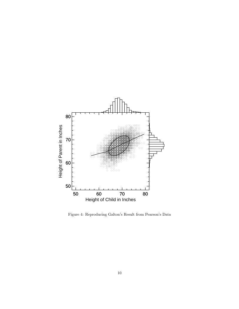
Can we pool Pearson’s data and get Galton’s result? Figure 4 shows childheights plotted against parent heights when daughter and mother heights havebeen multiplied by Galton’s adjustment factor of 1.08. With these blendeddata, the telltale bend at the lower end of the fitted loess regression is readilyapparent.

Finally, if we fit a piecewise linear model to the blended Pearson data, weget a significant breakpoint near the mean child height of 65 inches (p < .05).

3

4 Conclusion

Is there any chance that Galton and Pearson, with the statistical tools they hadavailable, could have discovered this anomaly? Galton smoothed his data witha two–dimensional rectangular counting kernel, the “naive method” describedby Silverman (1986), in order to regularize the ellipse he sought. But it maybe unreasonable to assume that Galton might have used a conditional localsmoother to assess the fit of his regression line and, further, to recognize whethera bend in the smoother was important. In their search for universal hereditarylaws, Galton and Pearson were driven by the linear model and the normaldistribution because the associated parameters had scientific meaning for themthat went beyond mere description.

Could Galton and Pearson have used their linear tools to detect an anomalyand avoid pooling? In the context of Galton’s linear regression model, we mightask if the mother data support a different regression slope from that of thefather data. Applying a simple 2x2 analysis of covariance, with child heightas the covariate, we find the test for homogeneity of slopes with respect toparent (mother/father) to be significant (p < .01), while the same test withrespect to child (son/daughter) is not significant. Although we should qualifyour conclusions because of within–family dependence in the observations, wefind scant support for pooling these data.

Galton was clearly sensitive to the problem of pooling data from disparategroups. He wrote, for example,

It clearly would not be proper to combine the heights of men belong-ing to two dissimilar races, in the expectation that the compoundresults would be governed by the same constants. (Galton 1869, p.29, cited in Stigler, 1986)

Galton was also sensitive to how gender differences in stature might affecthis conclusions.

I use the word parent to save any complication due to a fact appar-ently brought out by these inquiries, that the height of the childrenof both sexes, but especially that of the daughters, takes after theheight of the father more than it does after that of the mother. Mypresent data are insufficient to enable me to speak with any confi-dence on this point, much less to determine the ratio satisfactorily(Galton 1886, p. 250).

Pearson pursued this point further. Analyzing Galton’s data, he found thatthe father–son correlation was .40, the father–daughter was .36, the mother–son was .30 and the mother–daughter was .28 (Pearson, 1896). Pearson viewedthese correlations as consistent with Galton’s interpretation.

...both sons and daughters, on the average, take very considerablymore after their father than after their mother (Pearson, 1896, p.275).

4

But Pearson distrusted Galton’s correlations because of the informal natureof Galton’s sample. Pearson examined the corresponding correlations in thedata he and Alice Lee had collected. Pearson found all four of his correlationsto be approximately .50 (Pearson and Lee, 1903). From this failure to finddifferences among correlations in his own data, Pearson later concluded thatthe asymmetry in Galton’s data was due to mis–measurement:

I think it may well have been due to amateur measuring of staturein women, when high heels and superincumbent chignons were invogue; it will be noted that the intensity of heredity decreases asmore female measurements are introduced. Daughters would bemore ready to take off their boots and lower their hair knots, thangrave Victorian matrons (Pearson, 1930, page 18).

Although Pearson noted the almost equal correlations in his and Lee’s data,he did not emphasize the differences in standard deviations. In another context,Pearson noted that the standard deviations did differ

Comparing the standard deviations of fathers and sons, we see thatfathers and sons are within the limits of random sampling equallyvariable. On the other hand daughters’ standard deviations are inevery case sensibly larger than those of their mothers (Pearson andLee, 1903, page 371).

But Pearson did not note that the significantly lower standard deviationsfor the mothers might lead to nonhomogeneity of slopes among the four groupseven after multiplying the women’s data by 1.08. As we have seen, a test forhomogeneity of slopes on Pearson and Lee’s data fails to support pooling.

This is not the first, nor likely the last, example in which improper poolingcan lead to mis–specification. It is interesting, nevertheless, that one of themost famous datasets in the history statistics has kept its secret for so long.The secret survived Pearson’s close scrutiny perhaps because he, like Galton,was determined to pool the data in order to compute general heredity coeffi-cients. It also escaped the attention of those citing Galton’s as the pre–eminentregression dataset. When we set aside Galton and Pearson’s peculiar evolu-tionary arguments for a pervasive normal law of heredity, we are better ableto see disparity in the actual numbers. Prior expectations influence posteriorjudgments.

References

[1] Cleveland, W.S. and Devlin, S. (1988). Locally weighted regression analysisby local fitting. Journal of the American Statistical Association, 83, 596640.

[2] Galton, F. (1869). Hereditary Genius: An Inquiry into its Laws and Con-sequences.London: Macmillan.

5

[3] Galton, F. (1886). Regression towards mediocrity in hereditary stature.Journal of the Anthropological Institute of Great Britain and Ireland, 15,246263.

[4] Hinkley, D. (1971). Inference in two–phase regression. Journal of the Amer-ican Statistical Association, 66 , 736–743.

[5] Pearson, K. (1896). Mathematical contributions to the mathematical the-ory of evolution.III. Regression, heredity, and panmixia. PhilosophicalTransactions of the Royal Society of London, 187 , 253318.

[6] Pearson, K. (1930). The Life, Letters and Labours of Francis Galton, Vol.III: Correlation, Personal Identification and Eugenics . Cambridge Univer-sity Press.

[7] Pearson, K. and Lee, A. (1896). Mathematical contributions to the theoryof evolution. On telegony in man, &c. Proceedings of the Royal Society ofLondon, 60 , 273–283.

[8] Pearson, K. and Lee, A. (1903). On the laws of inheritance in man: I.Inheritance of physical characters. Biometrika, 2 (4) , 357–462.

[9] Silverman, B. W. (1986). Density Estimation for Statistics and Data Anal-ysis. London: Chapman and Hall.

[10] Stigler, S. M. (1986). The History of Statistics: The Measurement of Un-certainty before 1900. Harvard University Press.

[11] Stigler, S. M. (1999). Statistics on the Table: The History of StatisticalConcepts and Methods. Harvard University Press.

6

Figure 1: Galton’s Fitted Regression Model

7

60 65 70 75Height of Child in Inches

60

65

70

75

Hei

ght o

f Mid

-Par

ent i

n In

ches

Figure 2: SYSTAT plot of Galton’s Data with loess fit

8

50

60

70

80

Hei

ght o

f Fat

her

50 60 70 80Height of Daughter

50 60 70 80Height of Son

50

60

70

80

Hei

ght o

f Mot

her

Figure 3: Pearson’s Data

9

50 60 70 80Height of Child in Inches

50

60

70

80

Hei

ght o

f Par

ent i

n In

ches

50 60 70 80

50

60

70

80

Figure 4: Reproducing Galton’s Result from Pearson’s Data

10