G89.2247 Lecture 8 1

G89.2247Lecture 8

• Example of Random Regression Model Fitting

• What if outcome is not normal?

• Marginal Models and GEE

• Example of GEE for binary outcome

G89.2247 Lecture 8 2

Psychological Interpretation of Longitudinal Data

(Presentation at 2000 meeting of Society for Multivariate Experimental Psychology)

Niall Bolger

Pat Shrout

New York University

G89.2247 Lecture 8 3

Goals of SMEP Presentation

• Describe a Research Problem as a Case Study Design addressed advice from 1990Data available on www.psych.nyu.edu/couples

• Focus on interpretation of parameters that arise from application of general random regression methods to this problem

• Briefly describe new design issues

G89.2247 Lecture 8 4

A Case Study of a Longitudinal Application in Psychology

• Question: How does social support affect anxiety during a stressful event?

• Approach: Collect 30+ daily diary reports of support, coping and anxiety levels during acute planned stress event from members of couplesInquire about support provided by partnerInquire about support noticed by proband

• Acute Stressor: NY State Bar Exam

G89.2247 Lecture 8 5

The Bar Exam is Stressful

• About 30% of examinees will fail

• Most examinees work full time to prepare for exam in six weeks before the exam

• Much is at stakeEmployment requirementSelf esteem Social standing and esteemInvestment of time preparing

G89.2247 Lecture 8 6

Diary Reports Show Stress

• On average, steadily increases to day of exam

Anxiety over time

0.00

0.50

1.00

1.50

2.00

2.50

3.00

0 5 10 15 20 25 30 35

Days

PO

MS Mean

Var

G89.2247 Lecture 8 7

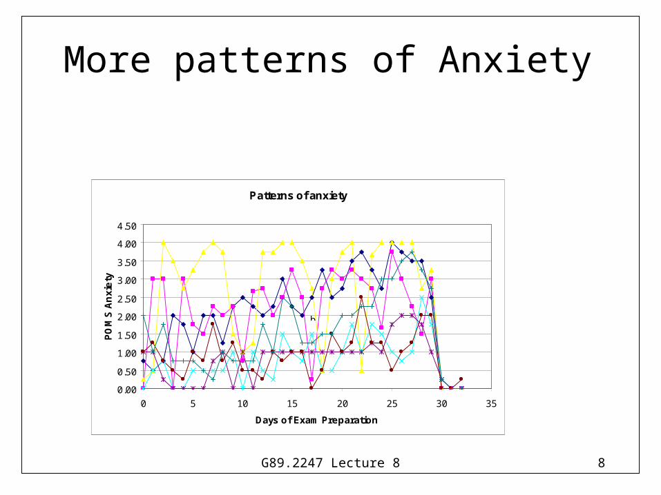
Individuals show variations of anxiety buildup

Individual patterns of change

0.00

0.50

1.00

1.50

2.00

2.50

3.00

3.50

4.00

4.50

0 5 10 15 20 25 30 35

Days of Exam Preparation

PO

MS

G89.2247 Lecture 8 8

More patterns of Anxiety

Patterns of anxiety

0.00

0.50

1.00

1.50

2.00

2.50

3.00

3.50

4.00

4.50

0 5 10 15 20 25 30 35

Days of Exam Preparation

PO

MS A

nxi

ety

b

G89.2247 Lecture 8 9

A Growth Model

Suppose we consider a simple linear growth model for each examinee. Anxiety at day t is represented as some baseline (intercept) plus an increment for the day in the series.

Model 1

Question: do persons who get more support over the 30 day period have different slopes?

ttTIt rTbbA

G89.2247 Lecture 8 10

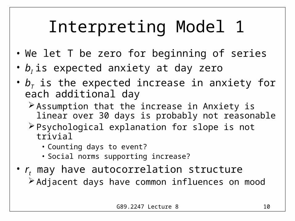
Interpreting Model 1

• We let T be zero for beginning of series• bI is expected anxiety at day zero• bT is the expected increase in anxiety for each

additional dayAssumption that the increase in Anxiety is linear over 30

days is probably not reasonablePsychological explanation for slope is not trivial

• Counting days to event?• Social norms supporting increase?

• rt may have autocorrelation structureAdjacent days have common influences on mood

G89.2247 Lecture 8 11

A Simple Intraindividual Model

• When support occurs, the trajectory may be affected. Theory says anxiety will be reduced. Data suggests the opposite for visible support.

Model 2

• Question: On days when support occurs does anxiety vary from expected trajectory?

ttStTIt rSbTbbA

G89.2247 Lecture 8 12

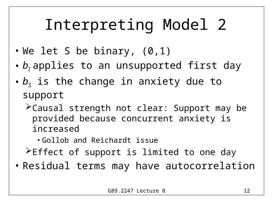
Interpreting Model 2

• We let S be binary, (0,1)

• bI applies to an unsupported first day

• bS is the change in anxiety due to supportCausal strength not clear: Support may be provided

because concurrent anxiety is increased• Gollob and Reichardt issue

Effect of support is limited to one day

• Residual terms may have autocorrelation

G89.2247 Lecture 8 13

An Autoregressive Model

• Anxiety tomorrow may be affected by processes other than support and time to exam. A basis for causal inference may be enhanced by adding autoregression term

Model 3• Question: Does support today affect anxiety

tomorrow, holding constant anxiety today as well as the expected trajectory?

ttAtStTIt rAbSbTbbA 1

G89.2247 Lecture 8 14

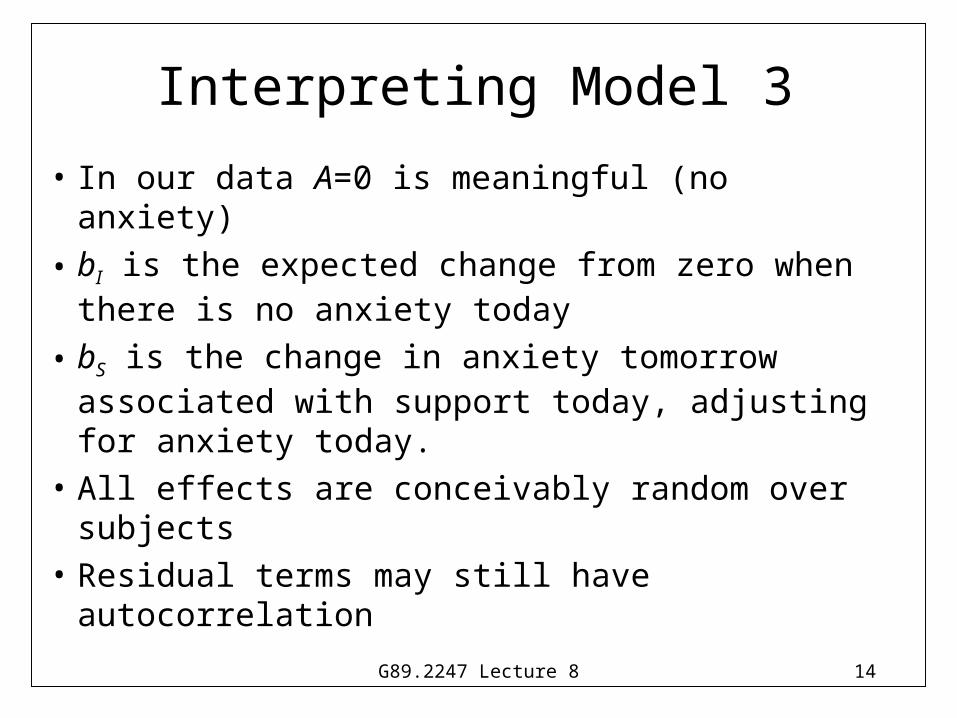
Interpreting Model 3

• In our data A=0 is meaningful (no anxiety)

• bI is the expected change from zero when there is no anxiety today

• bS is the change in anxiety tomorrow associated with support today, adjusting for anxiety today.

• All effects are conceivably random over subjects

• Residual terms may still have autocorrelation

G89.2247 Lecture 8 15

Interpreting the Autoregression Effect, bA

• Anxiety today may have structural effects on tomorrow that might be mediated by sleep (may be disrupted, adding to next day stress) relationships (may be impaired)preparation (may be disrupted)

• Anxiety today may be a proxy for additional effectsPoor expectations of achievement IllnessChronic stress buildup

G89.2247 Lecture 8 16

Some empirical results based on 68 couples over 30 days

• The Growth ModelB se

Intercept 0.9943 0.1751Diaryday 0.0341 0.0074MeanSupport 0.1229 0.2742Mean*Diaryday 0.0016 0.0116AR(1) 0.458

Random VarIntercept 0.32317Diaryday 0.00039Residual 0.551AIC -2262

G89.2247 Lecture 8 17

Simple Intraindividual Model on Lagged Support

B seIntercept 1.0503 0.0856Diary Day 0.0351 0.0036LagRecSup 0.0225 0.0383AR(1) 0.4558

Random VarIntercept 0.31510Diary Day 0.00039LagRecSup 0.00828Residual 0.548AIC -2261

G89.2247 Lecture 8 18

Autoregressive Model With Lagged Support, Phase and AR errors

B seINTERCEPT 1.2268 0.0969LagANX -0.1133 0.0247DIARYDAY 0.0330 0.0046PHASE 0.0864 0.0913LagSupp -0.0135 0.0382PHASE*LagSupp 0.2076 0.0898AR 0.530Random Effects VarINTERCEPT 0.36855LagANX 0.00955DIARYDAY 0.00045LagSupp 0.00165Residual 0.591AIC -2251

G89.2247 Lecture 8 19

Design innovations in ongoing work

• Respondents are asked to report POMS at waking in addition to bedtime

• Respondents are randomly assigned to diary, panel and cross-sectional arms

• POMS is refined to include more response categories

• Sample is recruited to be more heterogeneous

G89.2247 Lecture 8 20

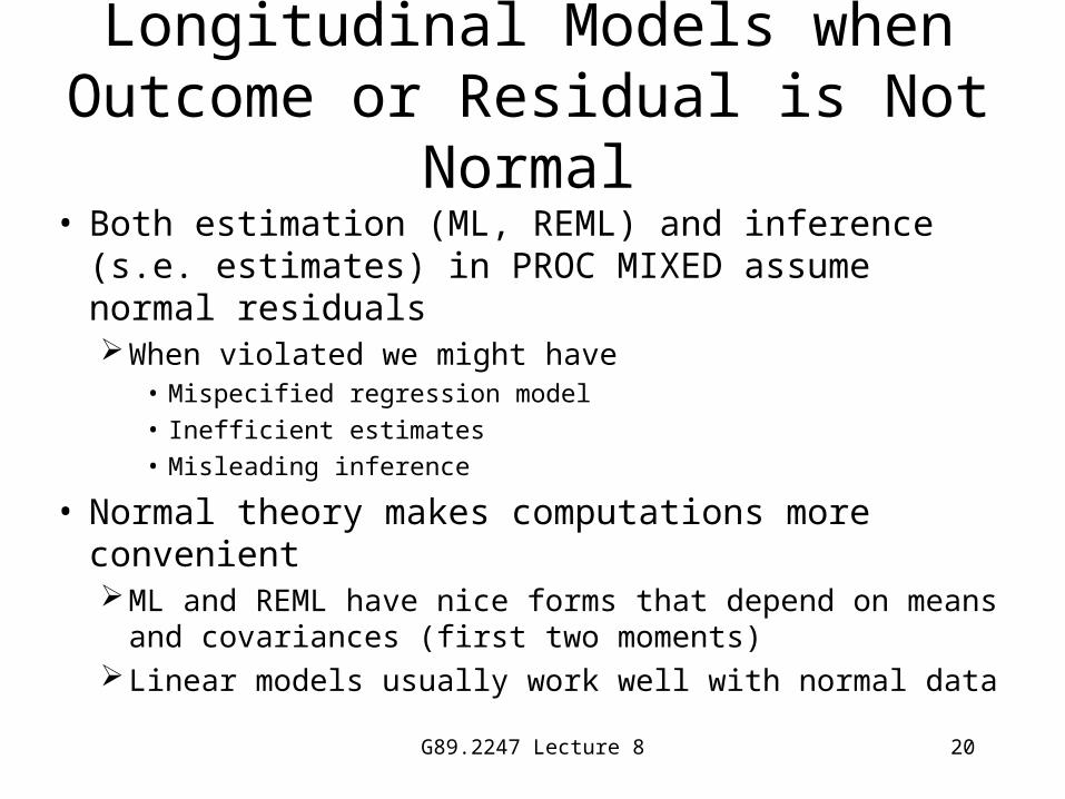
Longitudinal Models when Outcome or Residual is Not Normal

• Both estimation (ML, REML) and inference (s.e. estimates) in PROC MIXED assume normal residualsWhen violated we might have

• Mispecified regression model

• Inefficient estimates

• Misleading inference

• Normal theory makes computations more convenientML and REML have nice forms that depend on means and

covariances (first two moments)Linear models usually work well with normal data

G89.2247 Lecture 8 21

Mixed Models for Non-normal Outcomes

• Modeling non-normal outcomesBinary outcomes: logistic, probit regressionCount outcomes: Poisson regressionOrdinal outcomes: Multivariate probit, multinomial logistic

• Alternative models work best for large n• If number of time points is small, then level 1 (within

subject) models may be difficult to estimate• Special software is needed in any case

PROC NLMIXED (SAS)MIXOR, MIXREG (Hedeker and Gibbons)

G89.2247 Lecture 8 22

An Alternative Analysis: Marginal Models (GEE)

• If one is mainly interested in the fixed effects (population averages) then consider marginal modelsRandom effects are considered nuisance parametersModel is specified only for population (fixed) effectsResiduals are correlated because of individual effectsEstimates and inference take into account correlated

residuals

• Marginal Models ignore ZU in the mixed model

rZUWγY

G89.2247 Lecture 8 23

Example: Marginal Model From PROC MIXED

18 PROC MIXED NOCLPRINT COVTEST METHOD=REML;

19 CLASS id time;

20 MODEL anx=group week group*week /s;

21 REPEATED time /TYPE=UN SUBJECT=ID R RCORR;

22 TITLE2 'Fixed (Marginal Model): ASSUMES RESIDUALS HAVE GENERAL CORR PATTERN';

The Mixed Procedure Estimated R Correlation Matrix Row Col1 Col2 Col3 Col4 1 1.0000 0.7415 0.6336 0.6472 2 0.7415 1.0000 0.8051 0.7500 3 0.6336 0.8051 1.0000 0.8271 4 0.6472 0.7500 0.8271 1.0000

G89.2247 Lecture 8 24

Marginal effects: Taking Correlations Among R.Measures into Account

PROC MIXED (All fixed, R estimated to be Unstructured) Solution for Fixed EffectsEffect Estimate S. Error DF t Value Pr > |t|Intercept 1.1718 0.07454 133 15.72 <.0001group -0.6221 0.10580 133 -5.88 <.0001week 0.2733 0.02379 133 11.49 <.0001group*week -0.2944 0.03377 133 -8.72 <.0001

PROC MIXED (INTERCEPT, SLOPE RANDOM, AR(1) RESIDUALS) Solution for Fixed Effects Effect Estimate S. Error DF t Value Pr > |t| Intercept 1.1547 0.07482 133 15.43 <.0001 group -0.6028 0.1062 270 -5.68 <.0001 week 0.2642 0.02453 133 10.77 <.0001 group*week -0.2859 0.03482 270 -8.21 <.0001

G89.2247 Lecture 8 25

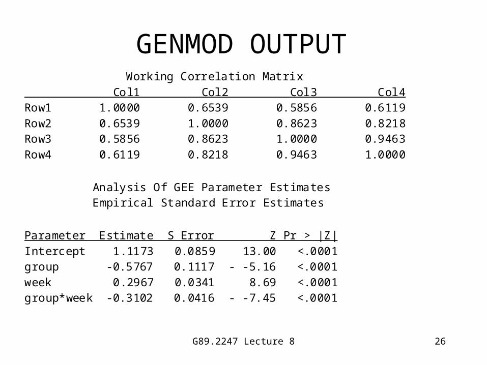
General Linear Models throughPROC GENMOD:

• A similar algorithm to the one used by PROC MIXED is available in GENMODWe can specify a structure for Var(Y|B)=VV is estimated and used to give weighted estimates of BGENMOD uses Generalized Score Estimation for V

PROC GENMOD; CLASS id; MODEL anx=group week group*week /DIST=normal; REPEATED SUBJECT=ID /TYPE=UN corrw; Title2 'GEE marginal repeated measures analysis'; run;

G89.2247 Lecture 8 26

GENMOD OUTPUT Working Correlation Matrix Col1 Col2 Col3 Col4 Row1 1.0000 0.6539 0.5856 0.6119 Row2 0.6539 1.0000 0.8623 0.8218 Row3 0.5856 0.8623 1.0000 0.9463 Row4 0.6119 0.8218 0.9463 1.0000 Analysis Of GEE Parameter Estimates Empirical Standard Error Estimates Parameter Estimate S Error Z Pr > |Z| Intercept 1.1173 0.0859 13.00 <.0001 group -0.5767 0.1117 - -5.16 <.0001 week 0.2967 0.0341 8.69 <.0001 group*week -0.3102 0.0416 - -7.45 <.0001

G89.2247 Lecture 8 27

The GEE Method of GENMOD can be used with Non-Normal Data

• Suppose we have a model h(Y) = X'Bwhere h() is a function that describes how Y is related to

X'B• E.g. If Y is binary (0,1) and P=Prob(Y=1), then h(Y) might be a

logistic function h(Y) = ln[P/(1-P)]

• h(Y) is called a LINK function

• Marginal models describe the relation between Y and X at the population level Instead of describing the average of random subjects’

models, it models the average response pattern.

G89.2247 Lecture 8 28

Example of GENMOD Analysis of Binary Outcome

• Modeling daily provision of practical support Is level of Anxious and Depressed Mood at waking related

to the provision of practical support on that day? Is there a tendency for partners to report more practical

support over the course of a diary study?

• We analyze binary reports of practical support provision over 28 days by 87 persons in our Grad Couple Study (comparison group in exercises)POMS Anxiety and Depression measured at wakingDiary day indicates course of study

G89.2247 Lecture 8 29

PROC GENMOD SETUP

• IRCPRP is binary received practical support The MODEL statement says that support will be modeled with a logistic

link function, and that day, AM-anxiety and AM-depression are predictors The variance structure is “exchangeable”, which is the same as the

sphericity or compound symmetry structure of MIXED. POMS Anxiety and Depression are on 0-4 scale.

filename myimport 'daysup.por'; proc convert spss=myimport out=sasuser.daysupp; TITLE1 'analysis of binary daily support'; run; proc genmod descending; class couple; model ircprp = day amanx amdep /link=logit dist=bin type3; repeated subject=couple /type=exch corrw; title2 'GEE marginal model of received practical support R=exch'; run;

G89.2247 Lecture 8 30

PROC GENMOD OUTPUT

• Logistic results say that odds of support at day zero for zero anxiety and depression is exp(-.60)=.55 (corresponding to p=.35)

• For each point increase of Anxiety, odds of support goes up by a factor of exp(.168)=1.18. Persons with values of 4 on Anxiety would have about 2 times the chance of support as persons at 0.

Analysis Of GEE Parameter Estimates Empirical Standard Error Estimates Parameter Estimate S Error 95% CI Limits Z Pr > |Z| Intercept -0.6033 0.1624 -0.9215 -0.2850 -3.71 0.0002 DAY 0.0138 0.0062 0.0016 0.0260 2.22 0.0263 AMANX 0.1684 0.0828 0.0060 0.3307 2.03 0.0421 AMDEP -0.1112 0.1181 -0.3427 0.1202 -0.94 0.3462