g-clamp programmer’s guide - university of pittsburgh
TRANSCRIPT

G-clamp Programmer’s Guide
version 1.2
Paul H.M. Kullmann and John P. Horn Department of Neurobiology and Center for the Neural Basis of Cognition
University of Pittsburgh School of Medicine E 1440 Biomedical Science Tower
Pittsburgh, PA 15261 http://www.neurobio.pitt.edu
To download this document and the G-clamp program go to: (http://hornlab.neurobio.pitt.edu)
Contact Information: Grant Support: This document and the G-clamp software that it describes were both developed at the University of Pittsburgh with support from National Institutes of Health grant RO1 NS21065. Copyright Information: These materials are freely available for non-commercial research and educational purposes. The authors reserve the copyright and request that others using this material acknowledge its origin. Those wishing to publish any of this material or to develop commercial applications must first contact the authors.
First Edition 2003, Revised, October 1, 2004 Copyright © 2004
Dr. Paul H.M. Kullmann Phone: 412-648-9291 [email protected] Dr. John P. Horn Phone: 412-648-9429 [email protected]

Kullmann and Horn (2004b) G-clamp Programmer’s Guide
Page 2 of 88
Table of Contents
1 Who should read this guide?....................................................................................... 4
2 Future direction of G-clamp development.................................................................. 4
3 Overview of G-clamp program architecture .............................................................. 6
4 The user interface: G-clamp.VI .................................................................................. 8
4.1 G-clamp start and program initialization ............................................................ 8 4.1.1 Initialize ...................................................................................................... 9 4.1.2 Initialize2 .................................................................................................. 11 4.1.3 Check Controls.......................................................................................... 13 4.1.4 Enable/Disable Controls ........................................................................... 15 4.1.5 PXI Target................................................................................................. 17 4.1.6 DAQ Board Configuration........................................................................ 18 4.1.7 Selection Modified.................................................................................... 18 4.1.8 Start ExpModule Step1............................................................................. 20 4.1.9 Start ExpModule Step2............................................................................. 20 4.1.10 Start Failed ................................................................................................ 22 4.1.11 New Data?! ............................................................................................... 22 4.1.12 Abort ......................................................................................................... 24 4.1.13 Process ...................................................................................................... 25 4.1.14 Stop ........................................................................................................... 31 4.1.15 Plot all ....................................................................................................... 31 4.1.16 Exit............................................................................................................ 32 4.1.17 Done.......................................................................................................... 32
5 An exemplar experiment module: IV Relation.VI.................................................... 33
5.1 Operation of the communication loop .............................................................. 35 5.2 IV Relation Sub.vi ............................................................................................ 35
5.2.1 The RT feedback module G-clamp DQA.vi ............................................. 39
6 Priorities and execution systems............................................................................... 44
7 Other experiment modules........................................................................................ 45
7.1 Gsyn Threshold................................................................................................. 45 7.1.1 read gsyn.vi ............................................................................................... 45 7.1.2 Gsyn Threshold Sub.vi.............................................................................. 46
7.2 Synaptic Gain.................................................................................................... 47 7.2.1 LoadTemplates.vi...................................................................................... 48 7.2.2 Synaptic Gain Sub.vi ................................................................................ 50 7.2.3 Write to Disk mod.vi................................................................................. 52
7.3 V-clamp............................................................................................................. 54

Kullmann and Horn (2004b) G-clamp Programmer’s Guide
Page 3 of 88
7.3.1 V-clamp Sub.vi ......................................................................................... 55
8 Other custom VIs ...................................................................................................... 56
8.1 AnalogInOutConfig.VI ..................................................................................... 56 8.2 List Templates.VI ............................................................................................. 56 8.3 SaveConfig.VI .................................................................................................. 59 8.4 ScriptAnalyzer.VI ............................................................................................. 60 8.5 TargetList.VI..................................................................................................... 62
9 Adding a new experiment module ............................................................................ 64
9.1 Creating the module.......................................................................................... 64 9.2 Adding the module to G-clamp.vi .................................................................... 65 9.3 New control parameters .................................................................................... 70
10 Non-LabVIEW files.............................................................................................. 71
10.1 RT FIFOs .......................................................................................................... 71 10.2 Read Time Stamp Counter - rdtsc..................................................................... 74 10.3 SetTimeDate ..................................................................................................... 75
11 LabVIEW RT specifics......................................................................................... 76
11.1 AI SingleScan's "sleep mode"........................................................................... 76 11.2 File I/O in LabVIEW RT .................................................................................. 79
12 Revisions............................................................................................................... 81

Kullmann and Horn (2004b) G-clamp Programmer’s Guide
Page 4 of 88
1 Who should read this guide?
This guide is intended for G-clamp users who have a basic knowledge of LabVIEW
programming, though not necessarily of LabVIEW-RT, and who want to develop a
custom experiment module or to make other program modifications.
The document focuses upon the operation of the main VIs (G-clamp.vi and the
experiment module VIs) and their custom sub-VIs. To illustrate how G-clamp works, we
follow program flow during an experiment. This approach takes the reader through
essential elements within the wiring diagrams. It also explains our rationale for choosing
certain programming structures over possible alternatives. Some of the decisions we
made in designing G-clamp simply reflect generally principles of efficient LabVIEW
programming and will thus be familiar to experienced LabVIEW programmers.
Hopefully these sections will also be helpful to those G-clamp users who are less
experienced in LabVIEW programming, yet wish to understand how the program works.
In addition to describing aspects of G-clamp that adhere to standard LabVIEW
conventions, this manual also stresses programming techniques that are specific to real-
time applications using LabVIEW-RT. In particular, we wanted to outline the concepts
that went into creating a dynamic clamp program that not only does the job, but that gets
maximum performance out of the hardware. Having made such a bold claim, we do not
wish to imply that G-clamp lacks room for improvement! Quite the contrary, we believe
that through continuing use in electrophysiology experiments, we and others will
discover limitations in the present program and ways to further enhance performance. In
this spirit, we encourage comments and suggestions for improvements in the program and
in the documentation that we have written.
2 Future direction of G-clamp development
Since its beginning in the spring of 2001, the G-clamp project has evolved through
numerous changes. Although the present version (1.2) is fully functional, the program
remains in a continuing state of development. This year, for example, we added a new

Kullmann and Horn (2004b) G-clamp Programmer’s Guide
Page 5 of 88
V-clamp experiment module so that one can conduct hybrid experiments that switch
between voltage-clamp and dynamic current-clamp modes. We have also supported
other users in modifying the existing experiment modules for their specific needs.
Several ideas under consideration for inclusion in a future release of G-clamp, version 2,
include:
- The ability to generate irregularly timed stimulus pulses that can drive nerve
stimulation and thereby mimic the activity represented by synaptic template files.
- The implementation of synaptic template files that can create multiple types of
virtual synapses, e.g. excitatory and inhibitory, NMDA vs AMPA-type kinetics
and voltage-sensitivity.
- Generation of an experimental logging function. This feature would
automatically generate a text file that contains a running record of all events in an
experiment, including the parameters used. It would also include a new
‘comments’ field that could be used to track additional information about the
experiment (e.g. drug-applications). The format of the log file could be either a
simple text file or a formatted file with fields whose content could be be bulk-
loaded into a relational database.
- Simplify the procedure for adding new experiment modules. This would require
changing the way in which experiment modules are integrated into the user
interface G-clamp.vi. At present, every experiment module is hard-wired into G-
clamp.vi and this requires making changes at several program locations into order
to add a new module. The revised program would simplify the process by
implementing a plug-in architecture. At program start, G-clamp.vi would scan the
plug-in directory for experiment modules and make them available for the user.
Thus would reduce to process of programming or modifying an experiment
module VI to the simpler task of writing the module and placing it in a plug-in
directory.
- Provide error/debugging information from program components executing on the
embedded computer during development of new experiment modules.

Kullmann and Horn (2004b) G-clamp Programmer’s Guide
Page 6 of 88
3 Overview of G-clamp program architecture
G-clamp, v1.2, consists of 2 parts that are divided between the host and embedded
computers:
1. The library G-clamp.llb resides on the host computer: G-clamp.llb contains G-
clamp.vi, which acts as the G-clamp user interface. G-clamp.vi is marked as a
top-level VI in G-clamp.llb and thus opens automatically when G-clamp.llb is
opened. The remaining files in G-clamp.llb, which are either standard LabVIEW
VIs or custom VIs, all operate as sub-VIs in G-clamp.vi.
2. The library Embedded.llb resides on the embedded computer: Embedded.llb
contains the VIs that constitute the experiment modules, the RT loop module and
the conductance modules. Embedded.llb also contains a set of standard and
custom VIs that are required as sub-VIs.
In the standard LabVIEW-RT architecture, as advertised by National Instruments, the
host computer acts only as a graphical interface for program development and as the
display of the VI front panel. For program execution, the code is automatically
downloaded to the embedded processor1. While this arrangement works well, it
constrains performance because some of the memory and other resources available on the
embedded processor must be dedicated to supplying display information to the host. In
order to maximize the embedded resources available for data collection and storage, we
employed an alternative programming method that involves LabVIEW being targeted to
the host computer, as opposed to the embedded processor. With LabVIEW targeted to
the host computer, the G-clamp.vi running on the host acts as a client that uses the VI
server of the LabVIEW RT Engine on the embedded computer to start and execute
experiment module VIs.
1 Compare Chapter 3 Software Overview/Programming LabVIEW-RT/Using the RT Development System with /Communicating Using Host LabVIEW Applications in the LabVIEW Real-Time User Manual.

Kullmann and Horn (2004b) G-clamp Programmer’s Guide
Page 7 of 88
In general, experiment module VIs are organized to perform two tasks in parallel (for
details and exceptions see the individual descriptions of the experiment modules3):
- execute a sub-VI that performs experiment-specific operations (e.g. loading a
template from file or analyzing an acquired trace to adjust parameters for the next
iteration) and the dynamic clamp by calling the RT Loop module VI, and
- use a dedicated TCP/IP connection to send acquired traces to and receive user
commands from the user interface VI.
While these two tasks are organized in parallel, the high execution priority of the RT
Loop module VI ensures that the dynamic clamp operation always takes precedence and
thus communication with the user interface VI occurs only in between iterations or after
the dynamic clamp experiment has finished.
Running the user interface on the host computer as a client for the experiment module
VIs running on the embedded computer as opposed to downloading and executing
everything on the embedded computer has advantages and disadvantages:
The main reason why this architecture was adopted was to be able to run dynamic clamp
experiments uninterrupted for several minutes and thus to preserve as much memory as
possible for templates used and traces acquired during such experiments4. The chosen
architecture aids in this goal by delegating the memory- (and time-) consuming process
of displaying traces to the host computer. It also allows for other memory- (and time-)
consuming processes like post-experiment analysis to be delegated to the host computer.
The main disadvantage of this architecture is that when LabVIEW is targeted to the host
computer it is not possible to apply LabVIEW debugging tools like probes, execution
highlighting etc. to experiment module VIs and their sub-VIs as these are executing on
the embedded computer.
3 Sections 3 and 5 4 Attempts to circumvent the problem of finite memory by performing file IO (loading the template and saving acquired traces) on the fly, i.e. while the experiment is in progress, were unsuccessful when running the dynamic clamp on a PXI-8170 controller at a feedback loop rate of 20 kHz. This might become an option in the future, when faster processors and/or hard drives become available.

Kullmann and Horn (2004b) G-clamp Programmer’s Guide
Page 8 of 88
4 The user interface: G-clamp.VI
G-clamp.vi is a queue-driven state machine: A While Loop loops continually as long as
G-clamp is running and executes exactly one case of a Case Structure during each
iteration. The selector determining which case to execute is a string derived from a
queue5, which operates as a FIFO buffer (first-in-first-out). If the queue is empty,
Remove Queue Element.vi times out after 1 ms and the default-case (“Check Controls”)
is executed. The main purpose of the default-case “Check Controls” is to detect user
interactions with front panel controls using an Event Structure and to add the appropriate
string to the queue. The Event Structure processes all defined user events that
accumulated before G-clamp.vi execution got to the Event Structure by executing the
appropriate event case(s). If no event occurred, the Event Structure waits for a certain
time before timing out and letting G-clamp.vi execution proceed.
Thus the architecture of G-clamp.vi as a queue-driven state machine ensures that G-
clamp.vi execution performs only required actions without wasting processor time on
executing currently unnecessary functions. Use of the Event Structure guarantees that no
user interaction goes undetected and is dealt with in the correct order while in the absence
of a user interaction waiting of the Event Structure until it times out (or an event occurs)
keeps G-clamp.vi idle and thus the host computer’s CPU free to perform other tasks.
The following sections will provide a detailed look at G-clamp.vi by systematically going
through individual cases of the state machine.
4.1 G-clamp start and program initialization
Code execution starts with creating the queue, inserting the string ‘Initialize’ into it and
with initializing several shift registers that are used to carry the values of several
variables from one iteration to the next of the large outer While Loop.
5 The queue-VIs used are LabVIEW 6.0-style which allow only strings to be used as queue elements. In LabVIEW 6.1 these VIs have been replaced with queue-VIs that allow any data type to be used.

Kullmann and Horn (2004b) G-clamp Programmer’s Guide
Page 9 of 88
4.1.1 Initialize
An Open VI Reference provided with the path of G-clamp.vi is used to obtain a VI
reference to G-clamp.vi. This reference is subsequently used to invoke methods
(reinitialize all front panel controls to their defaults) and to set properties (front panel
window title) of G-clamp.vi. For later use in other cases, the G-clamp.vi VI reference is
bundled into the corresponding cluster element of the large cluster that is passed from one
iteration of the outer While Loop to the next via the top shift register.
1. A VI reference to G-clamp.llb/TargetList.vi is obtained to invoke the method
‘Get Control Value’ on the control ‘PXI Target’. This control of TargetList.vi
contains all required information about the PXI controller last used6. The ‘Get
Control Value’-method returns a string, which has to be converted into a
meaningful data format. This is done by providing the Unflatten From String
function with a constant of the same data format as the control on which ‘Get
Control Value’ was invoked. After the Invoke Node has executed, the VI
reference to TargetList.vi is discarded with a Close LV Object Reference.
Again, for later use in other cases, the PXI target information is bundled into the
corresponding cluster element of the large cluster that is passed from one iteration
of the outer While Loop to the next via the top shift register.
2. The IP address of the PXI controller obtained in the previous step is now used to
establish a connection to the VI server of the LabVIEW RT Engine on the PXI
6 For why that information is available in the control ‘PXI Target’ see section 8.5 TargetList.VI

Kullmann and Horn (2004b) G-clamp Programmer’s Guide
Page 10 of 88
controller using an Open Application Reference. This reference enables Open VI
Reference to obtain a reference to Embedded.llb/List Templates.vi and to
execute List Templates.vi by invoking the method ‘Run VI’. After List
Templates.vi has stopped, G-clamp.vi invokes the method ‘Get Control Value’
on the controls ‘Available templates’ and ‘Virtual G’s’ of List Templates.vi.
Finally, the VI reference to List Templates.vi is closed. Any errors that might
occur during this process are reported by Simple Error Handler.vi.
The strings returned by the method ‘Get Control Value’ are unflattened. Some
further processing is required before the names of the available template files can
be made visible to the user by updating the property ‘ItemNames’ of the Listbox
control ‘Available templates’. Because the control ‘Virtual G’s’ of List
Templates.vi is an exact copy of the control on the ‘Virtual G’s’ page of the G-
clamp.vi front panel, the output of Unflatten From String can be used directly to
update the ‘Value’ property of the that control.
Again, for later use in other cases, the information about the virtual conductances
is bundled into the corresponding cluster element of the large cluster that is
passed from one iteration of the outer While Loop to the next via the top shift
register.
While steps 1 to 3 are in progress, G-clamp.vi prompts the user to specify the directory
on the host computer used for saving data files.

Kullmann and Horn (2004b) G-clamp Programmer’s Guide
Page 11 of 88
This information is also bundled into the corresponding cluster element of the large
cluster that is passed from one iteration of the outer While Loop to the next via the top
shift register.
An ‘Enable/Disable Controls’- and ‘Initialize2’-string are added to the queue.
While G-clamp.vi execution consequently proceeds with the ‘Enable/Disable Controls’-
case, it suffices here to say that this case will set the enabled-state of G-clamp.vi front
panel controls in accord to set parameters for the IV Relation experiment module. The
precise working of the ‘Enable/Disable Controls’-case is explained in section 4.1.4.
4.1.2 Initialize2
1. G-clamp.vi next retrieves the settings used last for usage and scaling of the
analog-in and analog-out channels. These are stored in the values of the controls
‘AI Cluster’ and ‘AO Cluster’ of G-clamp.llb/AnalogInOutConfig.vi. Thus a VI
reference is opened to AnalogInOutConfig.vi and the method ‘Get Control
Value’ is invoked on the controls ‘AI Cluster’ and ‘AO Cluster’. The obtained
strings are unflattened and the retrieved settings are stored in the corresponding
cluster element ‘AI Cluster’ and “AO Cluster’ of the large cluster that is passed
from one iteration of the outer While Loop to the next via the top shift register.

Kullmann and Horn (2004b) G-clamp Programmer’s Guide
Page 12 of 88
‘AI Cluster’ of the large cluster also contains ‘Processor speed (MHz)’ as sub-
element and “AO Cluster’ of the large cluster also contains ‘device #’ as sub-
element. The correct values for these sub-elements have been obtained already
(see section 2 in 4.1.1 Initialize) and are now overwritten with wrong settings
derived from AnalogInOutConfig.vi. To maintain the correct settings, these are
read out of the large cluster and used to replace the incorrect settings after ‘AI
Cluster’ and “AO Cluster’ are updated with the values from
AnalogInOutConfig.vi.
2. The final step in G-clamp initialization is the synchronization of date and time
between host computer and PXI controller. This is done by using a Call By
Reference Node to execute Embedded.llb/SetTimeDate.vi on the PXI controller
while at the same time providing it with the current host computer date and time
as start parameters.

Kullmann and Horn (2004b) G-clamp Programmer’s Guide
Page 13 of 88
To use a Call By Reference Node, Open VI Reference has to be provided with a VI
Refnum control. The VI Refnum control acts as a type specifier so that the Call By
Reference Node can take on a pattern of input and output connectors identical to
the connector pane of the VI to be called7.
For more information about SetTimeDate.vi see section 10.3.
4.1.3 Check Controls
This is the default case that executes whenever the queue is empty. The central element in
this case is an Event Structure, which handles 4 different kinds of user interactions with
front panel elements in 5 of its 6 cases:
1. ‘Clear Graph’ clears the graph in the ‘Synaptic Gain’ page by providing its
‘Value’ property with an empty array. The empty array also resets ‘fpre’ and
‘Gain’, two controls used as temporary data buffers and accessed here via Local
Variables.
2. Menu Selection (User) handles selections made from the G-clamp run-time menu.
A Match Pattern first determines whether a selection has been made from the
menu item ‘Function’. If this is the case, the front panel window title of G-
clamp.vi is updated to reflect the chosen experiment module, the variable ‘Exp
Type’ is updated accordingly and the queue is provided with the string
‘Enable/Disable Controls’. 7 An easy way to specify the correct type is to right-click while pointing on the VI Refnum control, select ‘Select VI Server Class > Browse…’ and to choose the VI that is to be called by the Call By Reference Node. Keep in mind that any change in the connector pane of the called VI requires a new type specification of the VI refnum control.

Kullmann and Horn (2004b) G-clamp Programmer’s Guide
Page 14 of 88
If the selected menu item does not reflect a change in experiment module, the
menu item tag is fed into the queue8, causing the case with the same name as the
menu item to be executed later.
3. ‘SelectTemplate’, ‘DeselectTemplate’ feeds the string ‘Selection Modified’ into
the queue whenever a template gets selected or de-selected on the ‘Templates’
page.
4. ‘start/stop’ reacts to the ‘Start F12’ button and provides the queue either with a
string causing the start of an experiment or its abortion.
5. ‘IV Relation’ reacts to mouse-up events in the graph on the IV Relation page. A
mouse-up event in this graph is dragging one of the cursors to a new position. The
only action of this case of the Event Structure is to calculate the leak resistance.
8 Custom run-time menus can contain user-defined menu items and standard LabVIEW menu items (= application items). Application items used in a custom run-time menu require no additional programming as they behave in the same way as in the standard LabVIEW menu.

Kullmann and Horn (2004b) G-clamp Programmer’s Guide
Page 15 of 88
This is done by using the property ‘Cursor Position:Cursor X’ and ‘Cursor
Position:Cursor Y’ to obtain the cursor coordinates9 and thus the endpoints of the
line for which the slope (i.e. leak resistance) is calculated.
6. The Timeout-case does not effect anything and serves only as a means to exit the
Event Structure without waiting indefinitely for a user event.
The time-out value for the Event Structure is dependent on the state of G-clamp:
If the queue already contains elements (checked by Get Queue Status.vi) or if the
Boolean variable ‘DAQ in process?’ indicates an ongoing experiment, the Event
Structure waits only 1 ms for a user event, thus allowing the pending actions to
proceed quickly (If a data acquisition is in process, the
queue receives the string ‘New Data?!’ after the Event
Structure has completed).
Otherwise the Event Structure waits for 250 ms.
4.1.4 Enable/Disable Controls
This case executes after a change of the experiment module to make those controls
necessary for the module visible and enabled while disabling or making invisible
9 This works because the cursors in the IV Relation graph are set up as ‘Snap to point’, i.e. wherever they get dragged by the user their x and y coordinates always snap to the closest data point.

Kullmann and Horn (2004b) G-clamp Programmer’s Guide
Page 16 of 88
unneeded controls. Thus this case mainly sets the property ‘Disabled’ and the property
‘Visible’ of many controls to new values. For many controls these settings are stored in
an array of clusters with one array element (cluster) containing the settings specific to one
experiment module. The correct cluster is obtained by an Index Array, which uses the
variable ‘Exp Type’ (set in the ‘Menu Selection (User)’ case of the Event Structure in the
default case “Check Controls”) to index the array.
Other experiment module-specific control properties that are set by the user (the cluster
of controls in the right part of the ‘Settings’ page which also contains hidden controls to
buffer the values of the controls ‘Gmin/1’, ‘Gmax/2’ and ‘Available templates’) are
stored in the 1-D array of cluster ‘ControlsBuffer’.

Kullmann and Horn (2004b) G-clamp Programmer’s Guide
Page 17 of 88
4.1.5 PXI Target
This case is invoked by the menu item ‘File > Preferences > PXI Target’ when the user
wants to change the PXI controller G-clamp targets.
After a type specifier VI Refnum to Embedded.llb/TargetList.vi has been obtained, the
property ‘Front Panel Window:Open’ of the VI is set to TRUE. A Call By Reference
Node is used to execute TargetList.vi, causing G-clamp.vi to wait until the user is
finished selecting a PXI controller and TargetList.vi stops. The Call By Reference Node
connector output ‘PXI Target’ is then used to update the corresponding element of the
large cluster that is passed from one iteration of the outer While Loop to the next via the
top shift register. Closing the VI reference does not close the front panel window of
TargetList.vi. Thus the VI and changes to its controls made by the user remain in
memory. After a new type specifier VI Refnum to Embedded.llb/TargetList.vi is
obtained10, the method ‘Make Current Values Default’ is invoked and these changes to
default values are made permanent by saving the VI with the method ‘Save Instrument’.
Finally the front panel window of TargetList.vi is closed and by closing the VI reference
the VI is removed from memory.
Selecting a new PXI controller for G-clamp requires re-initialization of G-clamp.vi. Thus
the queue is provided with the string ‘Initialize’. As ‘Initialize’ will create a new
application reference to the LabVIEW RT Engine on the newly selected PXI controller,
the old target application reference is closed.
10 The first type specifier VI Refnum control is set to the VI server class ‘Strictly typed VI’. This VI server class can not invoke the method ‘Make Current Values Default’. Therefore the second specifier VI Refnum control is set to the more general VI server class ‘VI’.

4.1.6 DAQ Board Configuration
This case is invoked by the menu item ‘File > Preferences > DAQ Board Configuration’
when the user wants to change the settings for the analog-input or analog-output channels
used.
This case operates analogous to the previously outlined case ‘PXI Target’ using
Embedded.llb/AnalogInOutConfig.vi (section 4.1.5 PXI Target).
4.1.7 Selection Modified
This case is executed after using
one of the two front panel controls
for selecting or deselecting a
template. Because the two controls
are associated with the same event-
case of the Event Structure in the
default case ‘Check Controls’ (see
section 4.1.3) and because they
have opposing
effects, it is sufficient to query only one (‘SelectTemplate’) of the two
controls in the ‘Selection Modified’ case.
The control ‘Available templates’ is a Listbox control whose output is a
1-D array of long integers (I 32) with each number reflecting the index of the currently
selected item(s). The indicator ‘Selected templates’ is a Table indicator whose output is a
2-D array of strings (only the first column of the table is visible).
- Selecting a template: The ‘Value’ property of ‘Available Templates’ is used to
index the 1-D array of strings which is the control’s property ‘Item Names’ (1).
The resulting 1-D array is appended (concatenated) to a 1-D array containing the
templates that had been selected earlier and that are visible in the indicator

Kullmann and Horn (2004b) G-clamp Programmer’s Guide
Page 19 of 88
‘Selected templates’ (2). This 1-D array has been obtained by using Reshape
Array to convert the 2-D array reflecting the ‘Value’ property of the indicator
‘Selected templates’ (which contains elements only along one dimension, i.e. the
first column) into a 1-D array (3). Lastly, the concatenated 1-D array is converted
back into a 2-D array using a Build Array to update the ‘Value’ property of
‘Selected templates’ (4).
- De-selecting a template: The property ‘Selection Start’ of the indicator ‘Selected
templates’ contains the row and column index of the beginning of the data
selection. The row index is obtained with an Unbundle and used at the row index
input (index 0) of a Delete From Array. Delete From Array takes the 2-D array
that is the ‘Value’ property of ‘Selected templates’ (containing elements only
along one dimension, i.e. the first column) and because its disabled column index
input (index 1) it deletes one (1 at length input) complete row.
12
3
4

Kullmann and Horn (2004b) G-clamp Programmer’s Guide
Page 20 of 88
4.1.8 Start ExpModule Step1
This case is preparatory and precedes the actual start of a data acquisition (‘Start
ExpModule Step2’).
- It transfers the values of several controls to corresponding elements of the large
cluster that is passed from one iteration of the outer While Loop to the next via the
top shift register.
- To free memory on the host computer it clears several data buffers and the trace
display by feeding them empty inputs.
- In case of the Gsyn Threshold and the Synaptic Gain module, it checks whether a
template has been selected. On this condition rests whether execution will proceed
with the ‘Start ExpModule Step2’ case.
4.1.9 Start ExpModule Step2
This case uses the application reference to the LabVIEW RT Engine on the PXI
controller11, which had been obtained in the ‘Initialize’ case to open a VI reference to the
experiment module VI. It then invokes the method ‘Set Control Value’ to provide the
experiment module VI with all the user-specific settings required for execution of the
experiment module. This process will be explained in more detail below. It next starts the
experiment module VI by invoking the method ‘Run VI’ with the parameter ‘Wait until
done’ set to FALSE. This allows code execution of G-clamp.vi to proceed without
waiting for the experiment module VI to finish. Lastly it uses Open TCP Connection to
establish a TCP connection with the experiment module VI that will serve to transfer the
acquired data from the experiment module VI on the PXI controller to G-clamp.vi on the
host computer. If all these actions occurred without an error, i.e. the ‘status’ variable of
the error cluster is FALSE, a string (‘Send Control Values’12) is fed into the queue.
Because no case ‘Send Control Values’ exits, the default case ‘Check Controls’ will
11 This is the reason why after a re-boot of the PXI controller G-clamp.vi also has to be re-started: Re-booting the PXI controller makes the application reference invalid and G-clamp.vi has to obtain a new one. 12 This is a leftover from a former case ‘Send Control Data’. Any string, including an empty string, could be used here to force execution of the default case ‘Check Controls’ next.

Kullmann and Horn (2004b) G-clamp Programmer’s Guide
Page 21 of 88
execute next. With the variable ‘DAQ in process?’ now TRUE ( = Not FALSE), the
queue will be provided in ‘Send Control Values’ with a string directing it to the case that
checks for the availability of new data (‘New Data?!’).
Transferring experiment parameters to the experiment module VI:
Related parameters (mostly derived from the large cluster that is passed from one
iteration of the outer While Loop to the next via the top shift register) are bundled
together in an array or a cluster that is then converted to the LabVIEW data type variant.
In the Case Structure all variants relevant to the selected experiment module are then
assembled into a 1-D array, which is used to auto-index (together with a 1-D array of
strings representing the control names) the For Loop in which the method ‘Set Control
Value’ is invoked on the experiment module VI.
While this scheme requires converting the parameters back into their original data types
in the experiment module VI, it offers a flexible way to deal with different types and
numbers of parameters required for different experiment modules:
- Changes to the number of elements in a cluster or array of related parameters are
taken care of automatically by the data type conversion to variant.
- Re-sizing the Build Array function and exploiting the auto-indexing of the For
Loop adjusts to changes in the number of variants.

Kullmann and Horn (2004b) G-clamp Programmer’s Guide
Page 22 of 88
4.1.10 Start Failed
Closes the TCP connection and the reference to the experiment module VI if an error
occurred in the ‘Start ExpModule Step2’ case.
4.1.11 New Data?!
Uses the first TCP Read to check whether data are available on the TCP connection. If
nothing is sent via the TCP connection, TCP Read times out after 1000 ms and the error
status of the ‘error out’ cluster of TCP Read is TRUE. The empty TRUE-case of the large
Case Structure executes and in the TRUE case of the small Case Structure the error code
is analyzed: Error code 66 indicates that the TCP connection was closed by the peer, i.e.
the experiment module VI. As the experiment module VIs close the TCP connection only
after they have finished transmitting data to G-clamp.vi, error 66 indicates that the data
acquisition is over, the experiment module VI has stopped and the ‘Stop’ case of G-
clamp.vi should be executed next. If the error code is not 66, it is assumed that TCP Read
simply timed out, i.e. the experiment module VI is running but not sending data right
now. In this case the ‘Check Controls’ case will execute next. Thus during an experiment
it takes up to 1000 ms before G-clamp.vi reacts to a user interaction on the front panel.
Because of the TRUE-status of the variable ‘DAQ in process’ (after handling the user
events) execution will return to the ‘New Data?!’ case as long as the TCP connection is
open.

Kullmann and Horn (2004b) G-clamp Programmer’s Guide
Page 23 of 88
If data are received, the first TCP Read reads 4 bytes. The Type Cast function is used to
convert the string output of TCP Read into a long integer (I 32). This number gives the
number of bytes to read with the second TCP Read. The string output of the second TCP
Read is Type Cast into a 1-D array of single precision numbers (SGL). Because each
experiment module VI sends two blocks of data with identical structure (see section
4.1.13 Process for details), the output of the third TCP Read is actually not needed
because the output of the first TCP Read is used again to set the number of bytes to read
for the last TCP Read. The output of the last TCP Read is also converted to a 1-D array of
SGLs and both arrays are combined to a 2-D array and temporarily stored in the hidden
indicator ‘Waveform Graph’. Finally, the small Case Structure directs G-clamp.vi to the
case ‘Process’, in which the received data will be processed and analyzed.

Kullmann and Horn (2004b) G-clamp Programmer’s Guide
Page 24 of 88
4.1.12 Abort
0. Uses the TCP connection and TCP Write to send the
running experiment module VI a Boolean TRUE Type
Cast to a string (of 1 byte) causing it to abort the ongoing
data acquisition13. This works only with experiment module VIs that perform a
series of repetitive data acquisitions, i.e. iterations, as the corresponding TCP
Read in the experiment module VI is located in the While Loop that runs parallel
to the RT feedback loop module in these VIs and that sends data to G-clamp.vi in
between iterations.
1. It uses Flush Queue.vi to empty the queue and then inserts
the string ‘Stop’.
2. It clears the indicator ‘Selected templates’ by setting
its property ‘Value’ to an empty 2-D array.
13 Because of the unwired timeout input, TCP Write times out after the default 25.000 ms. This means that in situations in which the While Loop in the experiment module VI needs more than 25.000 ms for an iteration, the Abort-command goes unnoticed.

Kullmann and Horn (2004b) G-clamp Programmer’s Guide
Page 25 of 88
4.1.13 Process
This case processes and displays the data sent by the experiment module VI in a Case
Structure, which has one case for each experiment module with code-intensive
processing split into different frames of Sequence Structures.
The processing logic of the data is the same in each experiment module case and will first
be illustrated using the IV Relation case. Second, experiment module-specific differences
will be explained.
1. General outline of data processing
The data to be processed are read out from the ‘Value’ property of the hidden
indicator ‘Waveform Graph’. As described in section 4.1.11 (‘New Data?!’),
‘Waveform Graph’ contains two rows of data assembled from two consecutive
transmissions via the TCP connection between the experiment module VI and G-
clamp.vi. The first row of data in ‘Waveform Graph’ represents the voltage trace
recorded by the experiment module preceded by a header containing additional
information about the experiment. The second row of data contains the recorded
current trace preceded by an identical copy of the header used with the voltage
trace.
1. Thus the first task in
processing the received
data is to separate the
trace from the header and
to extract the information
contained in the header.
This is done in a For
Loop, which uses auto-
indexing of the 2-D array
of DBLs to set the
number of iterations and to separate the two sets of data. Index Array is then used
to obtain individual values from the header. The data set is then reduced with an

Kullmann and Horn (2004b) G-clamp Programmer’s Guide
Page 26 of 88
Array Subset that chops off the leading portion of the data set. The output of
Array Subset consists of the rest of the header plus the trace. The remaining
header consists of information that is used in the form of a 1-D array. Thus a Split
1D Array can be used to separate this part of the header from the trace. The 1-D
array of DBLs representing the trace is then converted to the LabVIEW data type
waveform by feeding it into a Build Waveform together with two DBLs
representing the time when the trace was recorded (t0) and the time interval
between data points (dt) extracted from the header. Using auto-indexing for the
output of the For Loop, the voltage and current waveforms are assembled into a
1-D array of waveforms, which feeds directly into the waveform graph indicator
‘Waveform Graph’ on the front panel to display the two traces. All other header
information extracted twice in the For Loop exits the For Loop without auto-
indexing.
Note that the content of the header and its size differ between experiment
modules. Therefore the arrangement of operations performed in the For Loop
varies somewhat between the experiment module-specific cases of the Case
Structure in ‘Process’. (The case for the Synaptic Gain module differs even more
as in this module transfer of the recorded traces to the host computer is optional –
see ‘Synaptic Gain’ under ‘Experiment module-specifics’ below) All headers
contain – although at different positions within the header – the true sample
interval (going through a Reciprocal and fed into the front panel indicator ‘A-D
rate’) and the RT loop performance information (fed into the front panel indicator
‘RT Loop Info’).
2. The 1-D array of waveforms containing the voltage and
current trace is added as new element to a 2-D array of
waveforms that is buffered in the hidden waveform
indicator ‘Output Array’. After the experiment module VI
has finished executing, this buffer serves as the source for
displaying all acquired traces in the front panel waveform
graph (see section 4.1.15 Plot all) and optionally for saving the data to a file.

Kullmann and Horn (2004b) G-clamp Programmer’s Guide
Page 27 of 88
3. Data are written to file if two conditions are TRUE: The
front panel control ‘Save data’ is set to TRUE and the
experiment module VI has performed the user-specified
number of iterations. Thus data to be saved accumulate in
temporary buffers until the end of the experiment. Also, while
the control ‘Save data’ is read out each time the ‘Process’ case
executes, it matters only at the end of the experiment when the
last set of data is processed.
Filenames for the data file are created by the sub-VI
GetDatafileName.vi in the TRUE-case for saving data.
GetDatafileName.vi uses the Get Date/Time In Seconds
function to get the current time when it executes. Date and
time are converted to a string, which includes the proper file type extension for
the selected experiment module using Format Date/Time String. Thus date and
time in the file name reflect the end of the experiment.
2. Experiment module-specifics
- IV Relation:
The operations necessary to obtain the relation between injected current and
membrane potential are straightforward and easy to figure out. The two 1-D
arrays of DBLs ‘Voltage’ and ‘Current’ provide the xy-graph ‘IV Relation’ with
input and serve as buffers before the data get saved to file. ‘Voltage’ and
‘Current’ are re-initialized in the ‘Start ExpModule Step1’ case with an empty
array. Calculation of the leak resistance is done in the ‘IV Relation’ case of the
Event Structure in the case ‘Check Controls’, i.e. whenever the user moves the
cursors in the xy-graph.
Structure of the 1-D array of DBLs ‘Waveform Graph’:
o index 0: start time of the trace acquisition, coded as seconds elapses since
12:00 AM

Kullmann and Horn (2004b) G-clamp Programmer’s Guide
Page 28 of 88
o index 1: reciprocal of the actual sample rate (Hz) of the analog input
operation
o index 2: not used, set to zero
o index 3 – 6: RT loop performance information
o index 7 – n: voltage and current trace, respectively
- Gsyn Threshold:
The scaling factor used with the last received set of traces is fed into the
numerical indicator ‘G-scaling’ and into the waveform chart ‘Gsyn
ThresholdChart’. History length of ‘Gsyn ThresholdChart’ is set to 100 data
points. The 1-D array of DBLs ‘G’s’ serves as a buffer for the scaling factors
before they get saved to file and is re-initialized in the ‘Start ExpModule Step1’
case with an empty array.
Structure of the 1-D array of DBLs ‘Waveform Graph’:
o index 0: start time of the trace acquisition, coded as seconds elapses since
12:00 AM
o index 1: reciprocal of the actual sample rate (Hz) of the analog input
operation
o index 2: factor used for scaling the conductance template
o index 3 – (n – 4): voltage and current trace, respectively
o index (n – 3) – n: RT loop performance information
- Synaptic Gain:
The two 1-D arrays of DBLs ‘fpre’ and ‘Gain’ provide the xy-graph ‘Gain’ with
input and serve as buffers before the data get saved to file. ‘fpre’ and ‘Gain’ are
re-initialized with an empty array in the ‘Clear Graph’ case of the Event Structure
in the ‘Check Controls’ case, i.e. by the user with the control ‘Clear Graph’.
Because of the long templates possible with this experiment module, a)
transmission of voltage and current trace to the host computer is optional and
done via a separate TCP transmission in the ‘Process’ case and b) saving of the
traces to file occurs on the PXI controller while analysis results are saved in a
separate file on the host computer.

Kullmann and Horn (2004b) G-clamp Programmer’s Guide
Page 29 of 88
The two transmissions in the ‘New Data?!’ case are used for header information
only and each of the two transmissions has different content. The 2-D array of
DBLs ‘Waveform Graph’ thus has the structure:
o index 0; 0: mean presynaptic activity rate fpre (Hz)
o index 0; 1: gain
o index 0; 2: ending time of the trace acquisition, coded as seconds elapses
since 12:00 AM
o index 0; 3: reciprocal of the actual sample rate (Hz) of the analog input
operation
o index 1; 0 – 3: RT loop performance information
To instruct Synaptic Gain.vi to save the traces to
file and/or transmit the traces for display to G-
clamp.vi, the two Booleans ‘Save data’ and ‘Show
traces’ are assembled into an array and after
flattening to string sent with the TCP Write
function.
To have identical file
names for the data file
saved on the PXI controller
and the host computer, the
ending time (coded as
number of seconds since
midnight) of the trace
acquisition as determined
by the PXI controller is
used on both computers. The missing day of month information is obtained with a
Get Date/Time In Seconds and a Format Date/Time String.
Trace transmission: With each iteration of the outer For Loop one of the two
traces is received via the TCP connection. Transmission of the traces is broken
into smaller segments, thus allowing the user to monitor progress via the ‘Status’

Kullmann and Horn (2004b) G-clamp Programmer’s Guide
Page 30 of 88
indicator. The initial TCP Read in the outer For Loop serves to receive
information about the number of segments to expect next and to set the count
terminal of the inner For Loop. The inner For Loop works in the same way as
data transmission in the ‘New Data?!’ case: The first TCP Read receives
information about the number of bytes to read with the second TCP Read, i.e. the
segment length. Each received segment is immediately unflattened from string
and appended to a 1-D array of SGLs, which uses a shift register to maintain its
content from one iteration of the inner For Loop to the next. After a trace has
been received completely, the 1-D array of SGLs is converted to a waveform and
a 1-D array of waveforms is obtained using auto-indexing of the output of the
outer For Loop.
- V-clamp:
Structure of the 1-D array of DBLs ‘Waveform Graph’:
o index 0:start time of the trace acquisition, coded as seconds elapses since
12:00 AM
o index 1: reciprocal of the actual sample rate (Hz) of the analog input
operation
o index 2: not used, set to zero
o index 3 – (n – 4): voltage and current trace, respectively
o index (n – 3) – n: RT loop performance information

Kullmann and Horn (2004b) G-clamp Programmer’s Guide
Page 31 of 88
Each experiment module has its own data file format. These are documented in
the G-clamp User Manual.
4.1.14 Stop
- Closes the TCP connection and the reference to the experiment module VI.
- Adds a ‘Plot all’ to the queue if more than 1 iteration has been performed.
- Adds a ‘Start ExpModule Step1’ to the queue if two conditions are fulfilled:
o ‘Selected templates’ is not empty and
o the current experiment module is Gsyn Threshold or Synaptic Gain.
- Sets the variable ‘DAQ in process?’ to FALSE and thus stops the default case
‘Check Controls’ from adding a ‘New Data?!’ to the queue.
4.1.15 Plot all
Replaces the last set of acquired traces visible in the front panel waveform graph
‘Waveform Graph’ with the contents of ‘Output Array’ which acts as buffer for all
acquired traces. Because ‘Output Array’ is a 2-D
array and ‘Waveform Graph’ a 1-D array, the traces
have to be re-organized: In the resulting 1-D array
the first half of elements are the voltage traces and
the second half of elements are the current traces. In
the following For Loop the first half of traces (plots) is assigned to left (voltage) y-scale
of ‘Waveform Graph’ and the second half of plots to the right (current) y-scale. In
addition, each current trace is given the same color as its corresponding voltage trace.
These operations result in constant updating of the front panel display, which can be
annoyingly slow and time-consuming, even with relatively small data sets. To speed up
this process, Auto-scaling of the x-axis is disabled during these operations and minimum
and maximum of the x-axis of ‘Waveform Graph’ are set to display only a fraction of the
actual data and after all plot-operations have been performed the x-axis is set back to its
original range.

Kullmann and Horn (2004b) G-clamp Programmer’s Guide
Page 32 of 88
4.1.16 Exit
Saves the current settings for the virtual conductances so that these settings can be used at
the next start of G-clamp.vi. This is done by invoking the method ‘Set Control Value’ on
the control ‘Virtual G’s’ of Embedded.llb/SaveConfig.vi and then invoking the ‘Run
VI’ method with the parameter ‘Wait until done’ set to TRUE. After the VI reference to
SaveConfig.vi has been closed, the reference to the LabVIEW RT Engine on the PXI
controller is closed.
If the ‘Exit’ command was given while an experiment was in progress, the queue receives
the string ‘Abort’ followed by the string ‘Done’, otherwise only the string ‘Done’.
4.1.17 Done
Closes the VI reference to itself and destroys the queue. Besides selecting the ‘Done’
case, the output of Remove Queue Element.vi also stops the outer While Loop, thus
terminating G-clamp.vi.

Kullmann and Horn (2004b) G-clamp Programmer’s Guide
Page 33 of 88
5 An exemplar experiment module: IV Relation.VI
IV Relation.vi, Gsyn Threshold.vi and V-clamp.vi each perform a series of data
acquisitions (iterations) and therefore these three VIs have essentially the same structure
consisting of 2 processes that operate in parallel: A communication loop transfers data to
and receives commands from the host computer via a TCP connection and the real-time
feedback loop as the central component of the dynamic clamp. From the wiring diagram
of IV Relation.vi the communication loop is immediately recognizable as the large While
Loop. The real-time feedback loop is implemented as a sub-VI (G-clamp DQA.vi) in IV
Relation Sub.vi in the Sequence Structure below the While Loop. Data acquired by the
real-time feedback loop are transferred to the communication loop via the RT FIFO
queue ‘Result Data Queue’, while the RT FIFO queue ‘Control Values’ serves to provide
IV Relation Sub.vi and the real-time feedback loop with the essential experiment
parameters (for general information about RT FIFOs see section 10.1).
Before IV Relation.vi actually starts running, the calling VI G-clamp.vi sets the variant
controls ‘DAQ Control Values’, ‘Virtual G’s’, ‘AI Cluster’ and ‘AO Cluster’ by invoking
the method ‘Set Control Value’ (see section 4.1.9 Start ExpModule Step2).
Once IV Relation.vi starts executing, the variant ‘DAQ Control Values’ is converted to
its original data format by providing the Variant To Data function with the cluster

Kullmann and Horn (2004b) G-clamp Programmer’s Guide
Page 34 of 88
‘Controls’ at its type-input. The parameter ‘# of iterations’ is multiplied by 2 (for the
voltage and the current trace) and used to set up the number of elements in the RT FIFO
‘Result Data Queue’ with each element consisting of a 1-D array of SGLs of length ‘scan
rate’ multiplied with ‘sample duration’ plus header length (see section 4.1.13 sub-section
2. Experiment module-specifics). Thus the RT FIFO ‘Result Data Queue’ is capable of
storing the complete set of traces that will be acquired during the experiment14. The
whole cluster obtained from converting the variant ‘DAQ Control Values’ consists of 15
identical elements, i.e. DBLs and can thus be converted with Cluster To Array into a 1-D
array of DBLs. This conversion retains the ordering of elements in the cluster and thus
makes it possible to read out a specific element from the array with Index Array. The 1-D
array of DBLs is written to the RT FIFO ‘Control Values’ which consists of 10 (because
10 is the default value of the unwired size-input of RTFIFOCreate DBLA.vi15) 1-D
arrays of 15 DBLs.
TCP Listen.vi waits for up to 60 sec for G-clamp.vi (see section 4.1.9 Start ExpModule
Step2) to open a TCP connection on port 205516.
After these initialization steps the communication loop and IV Relation Sub.vi are ready
to start executing17.
14 In theory, the RT FIFO could be used to provide the communications loop with individual data points as they are acquired: Instead of using a queue whose elements are 1-D arrays of SGL (i.e. a complete trace), the queue would consist of individual SGLs (i.e. data points). The RT feedback loop would write a new element to the queue during each loop cycle and the communication loop could transmit individual SGLs or assemble a few SGLs into a short TCP transmission. Re-assembling of the SGLs or short stretches of SGLs would be done after reception by G-clamp.vi. With this scheme memory requirement for the RT FIFO and therefore RAM usage on the PXI controller could be much reduced provided that a) the communication loop can read the queue and transmit the data fast enough compared to the speed at which the RT feedback loop writes to the queue and b) the sleep modus for AI SingleScan.vi is set to TRUE in ni-rt.ini (see section 11.1 AI SingleScan's "sleep mode"; Following the G-clamp installation instructions given in the G-clamp User Manual the sleep modus should be set to FALSE to achieve faster maximum RT feedback loop rates). 15 For next revision: 10 is unnecessary. Provide a constant of value 1 as input. 16 For next revision: No EOC Error.vi in front of TCP Close Connection is unnecessary. 17 For next revision: The start of IV Relation Sub.vi should be made dependent on successfully establishing the TCP connection (and establishing ‘Result Data Queue’, which would make it possible to set the return existing-input of RTFIFOCreate DBLA.vi in IV Relation Sub.vi to TRUE instead of the default FALSE).

Kullmann and Horn (2004b) G-clamp Programmer’s Guide
Page 35 of 88
5.1 Operation of the communication loop The first process in the loop is to wait up to 250 ms for a TCP transmission from G-
clamp.vi of a single byte, which is then Type Cast to a Boolean. A Boolean TRUE is the
signal for IV Relation.vi that the user wants to stop the experiment and gave the Abort-
command (see section 4.1.12 Abort). Type Cast returns a FALSE if TCP Read receives
nothing and times out. An abort-signal is transmitted to IV Relation Sub.vi via the RT
FIFO ‘Control Values’: The ‘stop’ element of the cluster ‘Controls’ is set to 1 and after
Cluster To Array added to the RT FIFO queue.
The smaller While Loop within the communication loop performs a read on the RT FIFO
‘Result Data Queue’. If the queue has not been empty and if no Abort-command was
given the removed queue element (trace) is Type Cast to a string, the string length
determined and (after conversion to a string) added in front of the trace string and via a
TCP Write sent to G-clamp.vi. For each trace transmitted a counter is incremented to
stop the communication loop after all traces have been sent to the host computer.
Note that execution of the communication loop is preempted by the real-time feedback
loop, which has the highest execution priority to maintain determinism. Thus transfer of
data traces is usually limited to the period in between two data acquisitions (iterations).
5.2 IV Relation Sub.vi The …Sub.vi of an experiment module VI
1. sets up the RT FIFO queues ‘Control Values’ and ‘Result Data Queue’
2. sets up the data acquisition board for the intended analog input and output
operations
3. prepares the output signal to the recording amplifier by interpreting the user
settings with Build AO waveform.vi (or reading a template file with read
gsyn.vi in Gsyn Threshold Sub.vi or interprets the script with ScriptAnalyzer.vi
in V-clamp Sub.vi)
4. calls the RT feedback loop module G-clamp DQA.vi to perform a data
acquisition (iteration)

Kullmann and Horn (2004b) G-clamp Programmer’s Guide
Page 36 of 88
5. puts together the acquired traces with a header and adds it to the ‘Result Data
Queue’ so that the communication loop can send it via the TCP connection to the
host computer.
As IV Relation.vi is designed to perform a series of data acquisitions (iterations), tasks 3,
4 and 5 from the list above are done repetitively in a While Loop, while tasks 1 and 2
need to be done only once before the While Loop starts.
1. IV Relation Sub.vi first performs a read on the queue ‘Control Values’ to obtain the
settings for the experiment. Based on these settings
- a 1-D array of SGLs is initialized to
pre-allocate memory for the current
trace, passed into the While Loop
and on to the ‘Template Im Buffer’
input of G-clamp DQA.vi (Pre-
allocation of memory for the voltage

Kullmann and Horn (2004b) G-clamp Programmer’s Guide
Page 37 of 88
trace is done in the While Loop in Build AO waveform.vi).
- a 1-D array of cluster of 2 elements (U 32, U 32) is set up for the time stamps
obtained during each cycle of the real-time feedback loop from which later the RT
loop info is determined.
- the RT FIFO ‘Result Data Queue’ is set up.
The 2-D array of SGLs contains initial values for the state variables of
the activation and inactivation gates of the implemented virtual
conductances. This array is fed into the While Loop via a shift
register. Thus the first call of G-clamp DQA.vi starts with the state
variables at arbitrary values and it will take some time before the state
variables settle to ‘normal values’. At the end of each data acquisition, the last values of
the state variables are put out from G-clamp DQA.vi into the shift register of the While
Loop and used as the starting values for the next call of G-clamp DQA.vi. Note also that
the 2-D array is initialized with only 6 rows. If more than 6 virtual conductances are
implemented in V-dependent Conductances.vi another row has to be added for each
additional conductance. Otherwise the retrieval operation in V-dependent
Conductances.vi will return ‘Not a number’ and unpredictable results can happen.
2. The analog input and analog output hardware is set up once outside the While Loop
with AI Config.vi and AO Config.vi. DAQ Hardware Settings.vi provides the required
parameters by translating the variants ‘AI Cluster18’ and ‘AO Cluster’ into the
appropriate data types. AI Config.vi and AO Config.vi provide task IDs for the analog
input and analog output operations used in the real-time feedback loop module G-clamp
DQA.vi. These task IDs are re-used with each data acquisition (iteration of the While
Loop) as the associated operations are cleared by G-clamp DQA.vi at the end of each
data acquisition (iteration).
From the variants ‘AI Cluster’ and ‘AO Cluster’ DAQ Hardware Settings.vi also
provides the recording amplifier-specific scale factors for the analog input and output
signals to Build AO waveform.vi and G-clamp DQA.vi. 18 To use the variant/control ‘AI Cluster’ to get the info about the processor speed from G-clamp.vi to the experiment module VI is not very logical. It’s even confusing as it is a hidden element of the cluster control ‘AI Cluster’.

Kullmann and Horn (2004b) G-clamp Programmer’s Guide
Page 38 of 88
3. Build AO waveform.vi generates a scaled analog output waveform that will be added
to any output signal calculated by the real-time feedback module G-clamp DQA.vi due
to virtual conductances. Thus the waveform has as many data points as will be acquired
by analog input and send out by analog output. The loop iteration count provided by the
iteration terminal (i) of the While Loop is used by Build AO waveform.vi to increment
the current step.
4. The RT feedback loop module G-clamp DQA.vi acquires one data point at a time,
calculates the new command signal for the recording amplifier and outputs it. The
operations performed by this VI are detailed in section 5.2.1.
5. After the real-time feedback loop module G-clamp DQA.vi has finished executing, the
two acquired traces (voltage and current) are assembled into a 2-D array. In a For Loop
each trace together with other header information is used
to build a new 1-D array (For the exact content of the
header see section 4.1.13 sub-section 2. Experiment
module-specifics). This new array is then added to the
‘Result Data Queue’ from which the communication loop
reads it and transmits it to G-clamp.vi on the host
computer19.
19 While in G-clamp DQA.vi great care has been taken to use only pre-allocated memory buffers of exactly the required size (to avoid invocation of the LabVIEW memory manager and thus avoid violation of determinism) the treatment of the acquired traces here violates this principle: Each use of the Build Array function results in a memory duplication and the same is possibly true for the entry nodes of the For Loop. A better way would be to pre-allocate buffers of length # of data points + # of header elements. G-clamp DQA.vi would place a trace in array elements 0 to trace length – 1. After G-clamp DQA.vi a number of Replace Array Subset functions would replace the final array elements with the header information (thus in effect changing the header to a tail and requiring a corresponding change in the ‘Process’ case of G-clamp.vi). To get rid of the For Loop this would need to be implemented twice, once for the voltage trace and once for the current trace, each followed by its own RTFIFOWrite SGLA.vi which would need to be properly chained to preserve the correct alternating order of elements in the queue (voltage trace – current trace – voltage trace- current trace…). On the other hand the use of the For Loop auto-indexed by the 2-D array makes it easy to add additional channels for transfer to the host computer.

Kullmann and Horn (2004b) G-clamp Programmer’s Guide
Page 39 of 88
6. Finally, once the last data acquisition (iteration) is complete and the
While Loop stops, AO Write One Update.vi sets the analog output
channel used to 0. This serves as a fail-safe mechanism to prevent a last
current command used in the While Loop and different from 0 to persist as command
input to the recording amplifier.
5.2.1 The RT feedback module G-clamp DQA.vi The task of this module is to read from an analog input channel the membrane potential
of the cell under study, calculate the new current value through the virtual conductance(s)
and write the current command to an analog output channel. This task is repeated in a
While Loop for the length of the experiment at the rate specified.
Before the loop starts executing, three operations are performed:
- 1 is subtracted from ‘# of data points’. This value compared with the current loop
iteration count yields the stop-condition for the While Loop.
- AI Start.vi is called with its ‘number of scans to acquire…’ input set to 0,
indicating continuous data acquisition until the task is cleared with AI Clear.vi.
- The ‘actual scan rate’ output of AI Start.vi is converted to sample interval length
to provide the ‘dt (ms)’ input of V-dependent Conductances.vi.

Kullmann and Horn (2004b) G-clamp Programmer’s Guide
Page 40 of 88
Once AI Start.vi has been called, the data acquisition board reads the specified analog
input channels and performs analog-to-digital conversions at the specified rate. The result
of each analog-to-digital conversion is written to an onboard FIFO buffer20 from which
AI SingleScan.vi - triggered by the scan clock on the data acquisition board that times
the analog-to-digital conversions - retrieves one element at a time. At the first iteration of
the While Loop, AI SingleScan.vi reads the newest data from the FIFO buffer, effectively
flushing the buffer of all data that accumulated in it between execution of AI Start.vi and
the first call of AI SingleScan.vi. The ‘data remaining’ output of AI SingleScan.vi
indicates now an empty FIFO and gives a 0 which – via a shift register- is used during the
next iteration of the While Loop to set the ‘opcode’ input of to AI SingleScan.vi to read
the oldest data in the FIFO21. Thus ‘data remaining’ monitors whether the While Loop
keeps up with the speed at which the data acquisition board performs analog-to-digital
conversions. Even if for some reason the feedback loop transiently lags behind22, it is
able to ignore outdated data and to catch up by flushing the FIFO buffer and using only
the newest data.
Note that the ‘data in’ input of AI SingleScan.vi is set to a 1-D array with 2 elements, i.e.
an array with the same number of elements as will be put out by AI SingleScan.vi. This
improves performance of AI SingleScan.vi by pre-allocating a block of memory for the
data and thus avoiding invocation of the memory manager. The actual values in the 1-D
array meaningless and are ignored by AI SingleScan.vi.
The raw voltage data obtained from AI SingleScan.vi are converted to mV and pA. The
two values are stored separately in two 1-D arrays of SGL that had been initialized by
and passed to V-clamp DQA.vi by its caller IV Relation Sub.vi, ‘DC command Vm
Buffer’ and ‘Template Im Buffer’. Before the new values are stored in these arrays with
Replace Array Subset, from both arrays the element at index(current loop iteration count)
20 For the 16-Bit E Series Multifunction DAQ boards the length of this buffer is 512 samples. 21 We haven’t found anywhere an explanation for why it would make sense to read as often as possible the oldest data and to read the newest data (and flush the FIFO) only when necessary. We presume that reading from the head of the queue is still faster than flushing a queue and obtaining the newest element even if the queue contains only 1 element. 22 As long as the feedback loop does not lag that much behind that the constant analog-to-digital conversions result in an overflow of the FIFO buffer. In that case, LabVIEW restarts the data acquisition board, effectively canceling the analog input and output operations and thus probably get the While Loop stuck indefinitely.

Kullmann and Horn (2004b) G-clamp Programmer’s Guide
Page 41 of 88
is read out with Index Array. The element read out from ‘DC command Vm Buffer’
corresponds to the next DC current command set up by Build AO waveform.vi in IV
Relation Sub.vi and is summed up with the other currents through virtual conductances
calculated in the feedback loop. The element read out from ‘Template Im Buffer’ is 0
when V-clamp DQA.vi is called with the IV Relation module. When the Gsyn Threshold
or the Synaptic Gain module uses V-clamp DQA.vi, ‘Template Im Buffer’ contains the
conductance template read from file and already scaled by the respective …Sub.vi.
While the acquired current value is not used any further and simply stored in the buffer
‘Template Im Buffer’, the acquired voltage value is used to calculate the driving force for
the pre-determined conductance read from a template file and fed into V-dependent
conductances.vi23 to calculate the current through any active voltage-dependent virtual
conductances. Although analog output is performed on only 1 channel, AO Single
Update.vi requires a 1-D array of SGL at its ‘scaled data’ input. To transform the single
command value calculated in the loop into the required 1-D array without invoking the
memory manager, a pre-allocated (by feeding a constant into the While Loop) 1-D array
of SGL with only 1 element is used and a Replace Array Subset to exchange the constant
value with the calculated command value.
Because the ‘opcode’ input of AO Single Update.vi is set to ‘output & update’, AO
Single Update.vi sets the analog output channel to the new command value immediately
after having received the 1-D array. Thus the delay between acquiring the membrane
potential (analog input) and giving the adjusted current command (analog output)
depends only on the time it takes to perform the necessary calculations and consequently
varies depending on the combination of virtual conductances used. [It is possible to fix
the time interval between analog input and analog output by tying AO Single Update.vi
to the scan clock that controls the analog-to digital-conversions. This is done by replacing
AI Config.vi and AO Config.vi with AI control config.vi24 and AO control config.vi24
respectively. The main difference is that AI control config.vi has the ability to route
signals. By default it routes the AI scan start signal onto PFI7. AO control config.vi has
the ability to choose a clock source and specification. By default it chooses PFI pin as a
23 For a description of V-dependent Conductances.vi see section 9.1 of the G-clamp User Manual. 24 These VIs can be found in the library RT Control.llb that should be located in your …\LabVIEW 6.1\examples\real-time directory.

Kullmann and Horn (2004b) G-clamp Programmer’s Guide
Page 42 of 88
clock source, and 7 as the clock source specification. The result is that the analog input
scan clock is used to clock the analog output updates when the ‘opcode’ input of AO
Single Update.vi is set to ‘Output only’. This assures that each time a digital-to-analog
conversion is clocked in, the analog output is clocked out. Note that AI control config.vi
includes AI start.vi. and therefore the call to AI control config.vi should be the last
operation performed in …Sub.vi before G-clamp DQA.vi is called to prevent overflow
of the onboard FIFO25.]
After the analog output operation the Code Interface Node makes an assembly call to
read the Time Stamp Counter register off the Pentium-class processor and to obtain a
time stamp with a resolution at the frequency of the PXI controller’s CPU (see section
10.2). The time stamp is stored in a pre-allocated array for analysis after the While Loop
has finished executing. The execution order AO Single Update.vi - Code Interface Node
is achieved by placing the Code Interface Node into a Sequence Structure and by wiring
an output of AO Single Update.vi to it, thus forcing the Sequence Structure to wait until
the output of AO Single Update.vi is available.
After all shift registers have been updated, the While loop starts all over with AI
SingleScan.vi waiting for the next trigger from the scan clock. What happens during the
time until that trigger arrives depends on the setting for ‘UseSleepingTimedNonBuffered’
in the file ni-rt.ini on the PXI controller (see also section 11.1):
- If UseSleepingTimedNonBuffered=FALSE as is recommended in the G-clamp
installation instructions given in the G-clamp User Manual to achieve maximum
loop rates, the feedback loop will block all other processes running in parallel
(e.g. the communication loop) from proceeding. As the communication loop has
to wait for the end of a data acquisition (iteration) anyway before it can
communicate something to the host computer, this is not a loss.
- If UseSleepingTimedNonBuffered=TRUE, AI SingleScan.vi acts like a wait-
command until the next analog-to-digital conversion is triggered by the scan
clock. Until then the thread in which the feedback loop runs is effectively put to
25 Alternatively AI control config.vi can be broken apart into its constituent sub-VIs so that everything except AI Start.vi is performed once outside the While loop in …Sub.vi and AI Start.vi remains as the last operation before the While Loop in G-clamp DQA.vi (see also section 7.3.1 V-clamp Sub.vi for an example).

Kullmann and Horn (2004b) G-clamp Programmer’s Guide
Page 43 of 88
sleep and the PXI controller’s CPU is free to run other threads, e.g. the
communication loop.
Once the While Loop has finished, the analog input and output operations are cleared
with AI Clear.vi and AO Clear.vi. Most importantly, this stops the data acquisition
board from doing further analog-to-digital conversions and causing a FIFO overflow,
which would rest the whole DAQ board. Thus the tasks IDs handed down from …Sub.vi
can be re-used for the next data acquisition (iteration) without going through the whole
configuration process again.
Finally, the time stamps are analyzed to obtain the RT Loop Info. Before the 1-D array of
time stamps is handed to Timing Analysis.vi, the first 200 elements are chopped off with
a Delete From Array. This serves to eliminate intervals longer than the acquisition rate
bound to happen at the beginning of the data acquisition: It can take several cycles of the
feedback loop before all the hardware processes associated with analog input and output
are correctly initialized and working at a regular rate26.
26 For this reason LabVIEW-RT example-VIs usually set the ‘opcode’ input of AI SingleScan.vi to ‘read newest data’ for the first 10 cycles of the control loop. As these examples usually run at much lower speeds and G-clamp is supposed to go to maximum speeds, we thought it saver to discard more, but potentially extremely short cycles to give the system the time it needs before it runs regularly.

Kullmann and Horn (2004b) G-clamp Programmer’s Guide
Page 44 of 88
6 Priorities and execution systems
While the experiment module VI and thus the communication loop operate under
‘normal’ priority, the feedback loop - following general LabVIEW-RT programming
guidelines - executes with the highest priority level (time-critical priority). This can be
achieved by setting either the feedback loop module G-clamp DQA.vi to this priority
level or by setting the caller of G-clamp DQA.vi, the …Sub.vi within the experiment
module VI, to this level as sub-VIs automatically execute at the priority level of the
calling VI if the priority level of the calling VI is higher than the priority level of the
called sub-VI. In the G-clamp distributions v1.1 to v1.1.2 it is the …Sub.vi within the
experiment module VIs that have been set to ‘time-critical’ to ensure that not only the
feedback loop itself but also the timing between consecutive data acquisitions (iterations)
is under the strictest timing control.
While this makes sense as far as the five priority levels from ‘backgound’ to ‘time-
critical’ are concerned, it is unclear from National Instruments Application Note 144
(Using LabVIEW to Create Multithreaded VIs for Maximum Performance and
Reliability27) how the priority level ‘subroutine’ fits in under the conditions of a time-
critical process running under the real-time operating system of the PXI controller.We
have found that setting all sub-VIs used by G-clamp DQA.vi (LabVIEW system VIs and
custom VIs) to ‘subroutine’ allows higher feedback loop rates than setting them to
another level (which would be overridden by the ‘time-critical’ setting of the calling VI).
As far as the possible execution systems are concerned, in my opinion Application Note
144 doesn’t provide any useful information at all and again one is forced to simply
experiment with different settings.
27 Application Note 144 is available from NIs website or installed as \LabVIEW\manuals\ mltithrd.pdf

Kullmann and Horn (2004b) G-clamp Programmer’s Guide
Page 45 of 88
7 Other experiment modules
7.1 Gsyn Threshold
Gsyn Threshold.vi is essentially a clone of IV Relation.vi. The only difference is that
the number of data points per data acquisition (iteration) – which is required to create the
FIFO ‘Result Data Queue’ - is not derived from the variant ‘DAQ Control Values’ but
from the variant ‘Template’. ‘Template’ is converted to a string that gives the name of the
template file to be used and the file is opened and read with read gsyn.vi. Required
parameters as well as the template itself are transferred to Gsyn Threshold Sub.vi via
the RT-FIFOs ‘Control Values’ and ‘Result Data Queue’.
7.1.1 read gsyn.vi
read gsyn.vi first opens the template file for reading-only and then determines the length
of the file (in bytes) by calling EOF which returns the offset of end-of-file. The byte-
length of the file is divided by 4 as the template file contains only single precision
numbers (SGLs), i.e. 4 bytes/number. The first Read File returns the header of the
template by reading 19 SGLs from the beginning of the file. With the ‘pos mode’ and the
‘pos offset’ inputs unwired, the second Read File starts reading the template proper from
where the first Read File left the file mark when it finished. Note that the only
information actually used from the header is its first element, i.e. the sample interval.

Kullmann and Horn (2004b) G-clamp Programmer’s Guide
Page 46 of 88
7.1.2 Gsyn Threshold Sub.vi
Gsyn Threshold Sub.vi receives the template via the RT-FIFO ‘Result Data Queue’
before the While Loop starts executing. Scaling of the template is done within the While
Loop by multiplying the template with the mean of two shift registers initialized with the
user-specified values of the controls ‘Gmin’ and ‘Gmax’.
After a data acquisition (iteration) has been performed, the voltage trace is analyzed to
determine whether the virtual synapse elicited an action potential: Array Max & Min is
applied to the 1-D array and the maximum value is checked against 0. Thus the analysis
is a simple threshold comparison with the threshold value

Kullmann and Horn (2004b) G-clamp Programmer’s Guide
Page 47 of 88
hard-wired into the program as a constant. Note that an Array Subset is used to eliminate
the first 200 data points of the trace from the analysis. This eliminates any 0-crossings
that can occur as a consequence of initially arbitrary state variables when virtual voltage-
dependent conductances are used, especially when used together with a passive RC
circuit which has no sub-zero potential initially. Depending on the outcome of the
comparison, the content of either the ‘Gmin’ shift register or of the ‘Gmax’ shift register
is replaced with the scaling factor used for the previous data acquisition (iteration).
Note also that the While Loop contains Build AO waveform.vi, which is used in IV
Relation Sub.vi to generate the DC current command. This allows execution of a
template file in combination with a constant current injection.
7.2 Synaptic Gain
The architecture of Synaptic Gain.vi differs from the other experiment module VIs.
Synaptic Gain.vi executes a potentially very long template file a single time. Thus no
loop structure is required to repetitively transmit acquired data to the host and no RT
FIFO is used to transfer the acquired traces (voltage and current trace) from Synaptic
Gain Sub.vi to Synaptic Gain.vi. In addition, because transfer of very long traces to the
host computer can take a long time, it is optional. This necessitates a function to save
acquired traces on the hard disk of the PXI controller if the user wants to save the
acquired traces without having them transferred to the host computer.
Synaptic Gain.vi first builds paths to the template files and provides LoadTemplates.vi
with an array of SGLs containing the factors for scaling the templates.

Kullmann and Horn (2004b) G-clamp Programmer’s Guide
Page 48 of 88
Next the template length (number of data
points) is determined and memory for the
template is allocated by initializing a 2-D array
of SGLs. An EOF is used to determine the file
length (bytes divided by 4). Subtracting the
length of the header (128 SGLs = 512 bytes)
gives the template length as number of data
points. The template length is next divided by
5120 using Quotient & Remainder because the
template is going to be read from file and stored
in the 2-D array in chunks of 5120 data points28. If the remainder = 0, row size of the 2-D
array is set to the integer quotient, otherwise to integer quotient + 1. This number is also
fed into LoadTemplates.vi together with the remainder giving the number of elements in
the last data chunk and the header length (in bytes) of the template file.
7.2.1 LoadTemplates.vi
The outer large For Loop in LoadTemplates.vi executes once for each template file to
read. Its number of iterations is obtained by auto-indexing the 1-D arrays
‘ScalingFactors’ and ‘TemplateFilePaths’. It first opens a file for reading-only and reads
the first 19 SGLs, i.e. the header, into a 1-D array. From the header array it extracts
- the mean presynaptic activity fpre [Hz] (index 10)
- the length of the template [ms] (index 11)
- the time to wait after execution [sec] before starting another experiment (index 13)
- the sample interval [ms] (index 0)
- and the # of secondary synapses (index 9)
Because the first and the last of these parameters have different meanings depending on
the template file type, the type is determined by reversing the file name and comparing
28 For some unknown reason it was impossible to read very long template files and write very long data files in a single file read or file write operation. This problem could be overcome by repetitive reading/writing, i.e. breaking the data into chunks. 5120 is an integer multiple of 128. 128 data points (SGLs) are 512 bytes, which is the hard disk sector size in LabVIEW RT on a PXI controller. Thus 5120 was chosen to optimize file transfer rates (see section 11.2 File I/O in LabVIEW RT).

Kullmann and Horn (2004b) G-clamp Programmer’s Guide
Page 49 of 88
the first string element with ‘2’ (for *.gt2). For a pair of a gt1- and gt2-file, the fpre
values correctly reflect the mean frequency of events in the gt1-file and of events in the
gt2-file and are summed up in the For Loop. The number of secondaries can be ignored
in the For Loop iteration reading the gt1-file as the gt1-file reflects activity of one
synapse and 1 is added to the shift
register. During the second iteration of the For Loop, the number of secondaries in the
gt2-file is read out and added to the shift register. Thus ‘fpre (Hz)’ is obtained by
dividing the sum of presynaptic mean frequencies by the sum of synapses.
Note that the outputs ‘SampleInterval (ms)’, ‘PostWait (sec)’ and ‘TemplateLength (ms)’
reflect only the corresponding values found in the header of the last template file read
from a series of template files.
The smaller For Loop within the large For Loop reads
the template file in chunks of 5120 values (except the
last chunk which can be anything in between 1 and
5120). The For Loop uses a shift register to set the
read start position (‘pos offset’ input of Read File) to
the ‘offset’ output of the previous file read operation.
For the first iteration of the For Loop the shift register
is initialized with a constant of value 512. The chunk read is next multiplied with the
scale factor for the template file and summed up with the row in the 2-D buffer array that
it is going to replace. This buffer is maintained with a shift register from one iteration of
the large outer For Loop to the next. Thus by continuously updating this buffer the
memory requirement of reading and combining multiple template files is kept to the size
of the final template.

Kullmann and Horn (2004b) G-clamp Programmer’s Guide
Page 50 of 88
7.2.2 Synaptic Gain Sub.vi
Synaptic Gain Sub.vi converts the 2-D array with
the template into a 1-D array before it is handed to
G-clamp DQA.vi. This makes it easier to retrieve
individual array elements in the feedback control
loop as the only index required can be obtained
without any computation from the iteration (i)
terminal of the While Loop in G-clamp DQA.vi.
Changing the dimensionality of an array does not require a new memory allocation as the
number of elements stays the same and therefore the same memory space is reused.
Synaptic Gain Sub.vi also pre-allocates memory for the voltage trace to be acquired by
initializing a 1-D array of SGLs and for the time stamps collected in the feedback control
loop. Note that this 1-D array of cluster of unsigned long integers (U 32) is as long as the
template but does not exceed 1.000.000 elements. As it is unlikely that loop rates change
during a data acquisition, collecting more than 1 million time stamps will provide no
further information about deterministic execution of the control loop and the restriction to
1 million prevents excessive memory consumption by the time stamps. Thus although the
feedback loop will still collect a time stamp during each iteration, each value in excess of
1 million will be discarded.
Once G-clamp DQA.vi has finished, the acquired voltage trace is analyzed to determine
the number of action potentials elicited by the executed template. This is done with Peak
Detector PtByPt.vi. While the point-by-point analysis VIs are designed to be used in a
control loop by processing continuous
data streams one point at a time, they
require some overhead ultimately slowing
down a control loop that is supposed to
run as fast as possible. Note that the
accuracy of Peak Detector PtByPt.vi
depends on the ‘width’ input, which is set to a constant. Thus if ‘width’ is too narrow for
the width of an action potential at a given sampling rate, Peak Detector PtByPt.vi can
miss peaks.

Kullmann and Horn (2004b) G-clamp Programmer’s Guide
Page 51 of 88
After Synaptic Gain Sub.vi has finished, the results are communicated to G-clamp.vi
via the TCP connection:
1. Mean presynaptic frequency (‘fpre (Hz) output from LoadTemplates.vi),
synaptic gain (‘APs’ output of Synaptic Gain Sub.vi divided by total number of
presynaptic events), ending time of the experiment as seconds since 12:00 AM
and actual sample rate (elements 0 and 1 of ‘Output Array’ from Synaptic Gain
Sub.vi) are assembled in that order into a 1-D array of 4 elements, converted to a
string, the length of this string (also converted to a string) concatenated in front of
the string and sent via a TCP Write to G-clamp.vi.
2. In the same way, the ‘RT Info’ output of Synaptic Gain Sub.vi, which is also an
array of 4 elements, is converted to a string and communicated to G-clamp.vi.
With these two TCP Write operations of Synaptic Gain.vi, G-clamp.vi completes
execution of the ‘New Data?!’ case of its Case Structure and proceeds to the ‘Process’
case (see section 4.1.11).
3. Synaptic Gain.vi next waits for 25 seconds for a TCP communication from V-
clamp.vi (the unwired ‘timeout ms’ input of TCP Read defaults to 25000). The
corresponding TCP Write of G-clamp.vi occurs in frame 0 of the Sequence
Structure in the case processing Synaptic Gain data and indicates whether the user
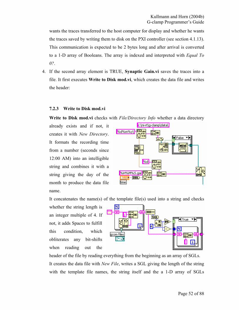
Kullmann and Horn (2004b) G-clamp Programmer’s Guide
Page 52 of 88
wants the traces transferred to the host computer for display and whether he wants
the traces saved by writing them to disk on the PXI controller (see section 4.1.13).
This communication is expected to be 2 bytes long and after arrival is converted
to a 1-D array of Booleans. The array is indexed and interpreted with Equal To
0?.
4. If the second array element is TRUE, Synaptic Gain.vi saves the traces into a
file. It first executes Write to Disk mod.vi, which creates the data file and writes
the header:
7.2.3 Write to Disk mod.vi
Write to Disk mod.vi checks with File/Directory Info whether a data directory
already exists and if not, it
creates it with New Directory.
It formats the recording time
from a number (seconds since
12:00 AM) into an intelligible
string and combines it with a
string giving the day of the
month to produce the data file
name.
It concatenates the name(s) of the template file(s) used into a string and checks
whether the string length is
an integer multiple of 4. If
not, it adds Spaces to fulfill
this condition, which
obliterates any bit-shifts
when reading out the
header of the file by reading everything from the beginning as an array of SGLs.
It creates the data file with New File, writes a SGL giving the length of the string
with the template file names, the string itself and the a 1-D array of SGLs

Kullmann and Horn (2004b) G-clamp Programmer’s Guide
Page 53 of 88
supplied by Synaptic Gain.vi
which contains other header
information. It uses the ‘offset’
output of the last Write File to
get the current length of the
file and if necessary it adds
bytes (I 8) to extend the file to
a length of 512 bytes. Having a header of 512 bytes means that subsequent
writing of the trace data starts with a new disk sector and therefore in the most
efficient way (see section 11.2 File I/O in LabVIEW RT).
Synaptic Gain.vi
next writes the traces
to file, first the
voltage trace and then
the current trace, by
breaking each trace
into smaller chunks
of 5120 data points
(or less for the last
chunk).

Kullmann and Horn (2004b) G-clamp Programmer’s Guide
Page 54 of 88
5. Only after the Case
Structure for saving the
data has completed does
the other Case Structure
for transmitting the data
to G-clamp.vi start
executing29. It transmits
each trace (starting with
the voltage trace) by
first transmitting a
number (a long integer (I 32) converted to a string, therefore 4 bytes) indicating
how many chunks of 5120 data points it will send before repetitively using TCP
Write to transmit one 5120 data points chunk at a time.
7.3 V-clamp
V-clamp.vi is essentially a clone of IV Relation.vi. The only difference is that the
number of data acquisitions (iterations) to be performed is not derived from the variant
‘DAQ Control Values’ but from the variant ‘Script’. ‘Script’ is first converted to a
flattened string and with an Unflatten
From String the script as seen on the
front panel of G-clamp.vi is obtained.
29 The reason for the sequential File I/O and TCP/IP is that we thought parallel execution might require duplication of the trace arrays. Theoretically this should not be the case, as neither operation changes the data and therefore LabVIEW should be able to use one copy of the data for both operations. We suspect that something else might reduce memory requirement and especially speed up these operations: According to a web presentation ‘Handling large data sets in LabVIEW’ given by an NI engineer, Damien Gray, and the accompanying handout ‘Large data objects in LabVIEW’ (both downloadable from NIs website as pdfs), tunnels used to route data sets through loops create a data copy each time the loop iterates. For Loops are used to break the File I/O and TCP/IP operations into smaller tasks done repeatedly. While we think that the same memory space is used over and over again as long as the size of the data set stays constant, it is possible that each creation of a copy – or memory allocation in other words – invokes the memory manager and thus slows down the whole process. This would explain the comparatively slow saving of data we observe in Synaptic Gain.vi, which is much slower than what we expected after making sure that writing is done in multiples of 512 bytes and which is much slower than the reading of the template file(s) at the beginning of the experiment. Damien Gray’s advice is to use shift registers, which will make a memory copy only the first time the loop executes.

Kullmann and Horn (2004b) G-clamp Programmer’s Guide
Page 55 of 88
A Match Pattern searches for the first occurrence of a string expression matching a
number in the script which is supposed to come in the first line after a ‘For’-command.
The unflattened script is also passed on to V-clamp Sub.vi for interpretation by
ScriptAnalyzer.vi.
7.3.1 V-clamp Sub.vi
V-clamp Sub.vi does not use the feedback loop module G-clamp DQA.vi. Instead a
simplified feedback loop is integrated directly into the While Loop of V-clamp Sub.vi
that executes once per data acquisition (iteration). The simplification consists of stripping
the feedback loop of any elements involved in the calculation of current through virtual
conductances, as virtual conductances are not used in voltage clamp. In addition, V-
clamp Sub.vi contains all configuration VIs required to tie the output of the command
signal by AO Single Update.vi to the scan clock. However, because the ‘opcode’ input
of AO Single Update.vi is set to ‘output and update’, these settings are ignored and
output of the command signal occurs as soon as AO Single Update.vi executes.

Kullmann and Horn (2004b) G-clamp Programmer’s Guide
Page 56 of 88
8 Other custom VIs
8.1 AnalogInOutConfig.VI
AnalogInOutConfig.vi contains two cluster controls that specify the settings for the
analog-input (‘AI Cluster’) and analog-out channels (‘AO Cluster’). Execution of
AnalogInOutConfig.vi follows the same logic as outlined for TargetList.vi (section
8.5): It waits until the user is finished and then updates the output cluster indicators ‘AI
Cluster’ and ‘AO Cluster’ from which G-clamp.vi derives the updated channel
information when AnalogInOutConfig.vi is called by the user via the menu ‘File >
Preferences > DAQ Board Configuration’. As with TargetList.vi, G-clamp.vi, will
invoke the method ‘Make Current Values Default’ and subsequently ‘Save VI’. This will
make any changes in the cluster indicators ‘AI Cluster’ and ‘AO Cluster’ permanent and
allow G-clamp.vi during initialization to obtain the information about the last PXI
controller by invoking the method ‘Get Control Value’ on the ‘AI Cluster’ and ‘AO
Cluster’ indicators of AnalogInOutConfig.vi (see 4.1.2 Initialize2).
8.2 List Templates.VI
In Embedded.llb.
List Templates.vi performs 3 functions:
1. It returns a list of available conductance modules. Because the order of modules
in this list has to reflect the order in which the conductance module VIs are
implemented in V-dependent Conductances.vi, assembling the list involves
several steps. The process starts with letting
Create Plugin List.vi search the library
Embedded.llb for all VIs with type
specifier unique
for conductance
module VIs

Kullmann and Horn (2004b) G-clamp Programmer’s Guide
Page 57 of 88
(Create Plugin List.vi30 uses Open VI reference and the provided type specifier
to open every VI in Embedded.llb. Open VI reference will return an error with
every VI of a different type, i.e. with every VI that has a different connector
pane).
Before the list of conductance modules is sorted into the correct order, the settings
for each conductance are retrieved from the configuration file Embedded.cfg. For
each conductance module the content of the string control ‘VI Label’ is obtained.
This string identifies a conductance in the front panel control ‘Virtual G’s’ of G-
clamp.vi to the user and it serves here as the section name for that conductance’s
entries in Embedded.cfg. If an entry for a conductance exists in Embedded.cfg,
the bundled settings for a conductance are added to a growing 1-D array of
clusters. A 1-D array of all the VI
labels is passed to the next For Loop
in which it is compared with a 1-D
array obtained from Get Section
Names.vi and containing all section
names in Embedded.cfg. A new 1-D
array is built containing only those
section names corresponding to
conductance modules and in the same
30 Create Plugin List.vi is a slightly modified version of an example VI downloaded from a National Instruments website illustrating how to program a plug-in architecture in LabVIEW.

Kullmann and Horn (2004b) G-clamp Programmer’s Guide
Page 58 of 88
order as in Embedded.cfg, i.e. in the same order as the conductance modules are
supposed to be used in V-dependent Conductances.vi. This still leaves open the
possibility that a new conductance module has been found by Create Plugin
List.vi for which no entry in Embedded.cfg yet exists. In this case the depleted 1-
D array of VI labels is not empty, i.e. has a length of >0 and the TRUE case of the
next Case Structure executes.
Another cluster is added to the 1-D array of
clusters containing the conductance
settings found in Embedded.cfg with the
cluster element ‘VI Label’ set to the first
element remaining in the 1-D array that
triggered execution of the TRUE case.
Likewise, the 1-D array of section names
created in the previous For Loop is
expanded by one element. Lastly, an entry for the new conductance module is
made in Embedded.cfg.
Note that this expansion of the 1-D array of clusters takes care of only one new
conductance module. If more than one new conductance module was created,
only the first one found by Create Plugin
List.vi will show up on the front panel of
G-clamp.vi irrespective of whether that
one was actually the first new one
implemented in V-dependent
Conductances.vi.
Finally, the 1-D array of clusters is re-
organized based on the order of elements in
the 1-D array of section names.
2. It returns a list of available template files by searching the directory c:\ni-rt\g-
clamp\template on the PXI controller for files of type *.gty and *.gt1. It does not
check whether a corresponding *.gt2 file exists for each *.gt1 file found. The list

Kullmann and Horn (2004b) G-clamp Programmer’s Guide
Page 59 of 88
is available in the string indicator ‘Available templates’ with file names separated
by a Tab Constant.
3. It resets both analog output channels by outputting a 0 voltage. This is in case that
the output registers for both channels took on some arbitrary values as can happen
after starting the PXI controller. It also performs a short data acquisition on
analog input channels 0 and 1 which apparently31 is required to initialize the
analog input hardware after the PXI controller has been started.
This function has a serious flaw32: The control ‘device (1)’ which provides AI
Config.vi and AO Config.vi with the device number of the installed DAQ board
is not updated at all. Thus correct functioning of the reset process depends on
having set the default value of the control ‘device (1)’ to the correct number for a
given PXI controller.
8.3 SaveConfig.VI
This VI is part of Embedded.llb. It
writes the settings for the virtual
conductances to the configuration
file Embedded.cfg on the PXI
controller. Note that Write Key.vi
does not actually write to file but
only predisposes a key for writing.
To achieve the actual write
operation, the ‘write
configuration file?’ input of
Close Config Data.vi has
to be set to TRUE.
31 We observed that without this analog input operation during G-clamp initialization the first real data acquisition performed by G-clamp as an experiment will result in bogus values. 32 For next revision: This can be fixed with an Invoke Method: Set Control Value in the ‘Initialize’ case of G-clamp.vi right before ‘Run VI’ is invoked.

Kullmann and Horn (2004b) G-clamp Programmer’s Guide
Page 60 of 88
8.4 ScriptAnalyzer.VI
This VI is part of Embedded.llb. It analyzes the voltage command script in the V-clamp
module and builds the command signal, which is then output to the recording amplifier.
Interpretation of the script requires identification of the commands and the numerical
values that follow almost all commands. As the whole script is a single string, the string-
functions Match Pattern and Fract/Exp String To Number are used in a repetitive
manner: Match Pattern finds the first number in the string by searching for a regular
expression defining a number (see ‘Description of reg. expression’ in Figure 8.1). The
string is then split into
- a substring with all characters before the number (command + a Space),
- a substring with all characters making up the number and
- a substring with everything after the number (remainder of the script).
The string making up the number is then converted to a numerical value with Fract/Exp
String To Number.
Figure 8.1
The first time this mechanism is employed, ScriptAnalyzer.VI expects the for-
command. Thus obtaining the substring with all characters before the number is actually
unnecessary and the corresponding output of Match Pattern as shown in Error!
Reference source not found. is unwired. In this instance, ScriptAnalyzer.VI only uses
the numerical value to set the count (N) terminal of the large For Loop to the intended
number of iterations.
The remainder of the script-string is then analyzed by repeating this basic mechanism
again and again. In most cases, i.e. whenever the script continues in a new line, the first

Kullmann and Horn (2004b) G-clamp Programmer’s Guide
Page 61 of 88
character in the remaining script-string is a Line Feed (LF) or33 Carriage Return (CR). To
get rid of this character, the String Subset function is employed (Figure 8.2):
Figure 8.2
After having determined the number of iterations, ScriptAnalyzer.VI proceeds with
determining the total length of the intended command sequence. This is done in a While
Loop by summing up all numbers following a wait-command. After the number of
iterations and the total command length has been determined, a 2-dimensional array for
the command-signal is initialized with zeroes. Obtaining the first wait-value of the script
initializes a pointer indexing the position from which to start replacing the zeroes with a
new voltage value.
After the first two lines of the script have been interpreted, the remainder of the script
enters the large For Loop (# of iterations) and the enclosed While loop. The While loop
operates on the presumption that the remaining script consists of a repetition of the
sequence:
- voltage-change-command
- increment/decrement-command (optional) and
- wait-command.
Thus the 1st Match Pattern determines the voltage command type (const=step change or
ramp). If the 2nd Match Pattern finds an increment or decrement command next, the
numerical value of the 1st Fract/Exp String To Number is incremented/decremented by
the numerical value of the 2nd Fract/Exp String To Number multiplied with the iteration
(i) terminal of the large For Loop. The next command is supposed to be a wait-command,
thus the 3rd Match Pattern is used only to interpret the next numerical value, which
specifies the duration of the new command voltage.
Having obtained all necessary information for this section of the script, a Replace Array
Subset updates the zero-values of the corresponding part of the 2-D command array to the
intended voltage values. 33 We simply haven’t bothered to figure out the exact cause.

Kullmann and Horn (2004b) G-clamp Programmer’s Guide
Page 62 of 88
The large For Loop stops once the 1st Match Pattern finds an end-command or if the
offset-past-match output returns –1, indicating that no regular expressions satisfying the
criteria for a match have been found.
8.5 TargetList.VI
TargetList.vi contains a 1-D array of cluster with each cluster containing necessary data
about one available PXI controller. Execution of TargetList.vi consists of waiting for
user input to either
- extend the array by one element with information about a new PXI controller
- remove a PXI controller by deleting the corresponding element from the array
- finish execution and writing information about the selected PXI controller to the
indicator ‘PXI Target’.

Kullmann and Horn (2004b) G-clamp Programmer’s Guide
Page 63 of 88
The caller of TargetList.vi, G-clamp.vi, will invoke the method ‘Make Current Values
Default’ and subsequently ‘Save VI’. This will make any additions to or deletions from
the list of PXI controllers contained in the 1-D array of cluster permanent as well as any
changes in a cluster element. This also allows G-clamp.vi during initialization to obtain
the information about the last PXI controller by invoking the method ‘Get Control Value’
on the ‘PXI Target’ indicator of TargetList.vi (see 4.1.1 Initialize).
Note that the time-out input of the Event Structure is unwired, i.e. the Event Structure
never times out. It will wait until a user event occurs, thus keeping G-clamp idle and the
computer CPU free to do other things.

Kullmann and Horn (2004b) G-clamp Programmer’s Guide
Page 64 of 88
9 Adding a new experiment module
For purpose of illustration the new experiment module will be named NewModule.vi
throughout this section. The discription will first focus on a new experiment module that
does not require new parameters and therefore new front panel controls on the user
interface (sections 9.1 and 9.2). Implementation of new parameters requiring additional
front panel controls on G-clamp.vi will be discussed in section 9.3.
9.1 Creating the module
The easiest way to create a new experiment module is to duplicate an existing module
and modify it. Because path information to sub-VIs is stored with the calling VI and the
LabVIEW RT run time engine on the PXI controller is not able to find a sub-VI in the
library Embedded.llb if the path does not explicitly point into the library, We strongly
recommend the following procedure:
- Copy Embedded.llb from the PXI controller to a directory c:\ni-rt\g-clamp on
your host computer, i.e. paths to Embedded.llb are identical on the host computer
and on the PXI controller. You are also going to need a directory c:\ni-rt\g-
clamp\gModules on the host computer that contains the conductance module VIs
(gNa.vi, gKdr.vi,…) implemented in Embedded.llb\V-dependent
conductances.vi.
- Temporarily remove or rename all other copies of Embedded.llb on the host
computer. If you rename them, rename the extension ‘llb’ because that is what
identifies it to LabVIEW as a LabVIEW library. The reason for making all other
Embedded.llb copies on the host computer “invisible” to LabVIEW is, to prevent
any accidental loading by the new experiment module VI of one of its a sub-VIs
from one of these Embedded.llb copies that have a directory path different than
c:\ni-rt\g-clamp.
- Open the experiment module VI you want to use as a template from c:\ni-rt\g-
clamp\Embedded.llb and save it immediately under a new name
(NewModule.vi) back into Embedded.llb with File > Save As…

Kullmann and Horn (2004b) G-clamp Programmer’s Guide
Page 65 of 88
- Modify NewModule.vi so that it performs your experiment.
- Use File > Save with Options… to save the final version of the experiment
module in Embedded.llb. Use the Custom Save option and save the entire
hierarchy including vi.lib files and external subroutines. With this custom save all
LabVIEW system libraries and external subroutines not present on the PXI
controller and used by NewModule.vi are added to Embedded.llb34.
- Copy Embedded.llb back into c:\ni-rt\g-clamp on the PXI controller.
9.2 Adding the module to G-clamp.vi
1. From the G-clamp.vi menu use Edit > Run-Time Menu… to start the menu
editor. Under the menu item ‘Function’ add the name of the new experiment
module (without the extension ‘.vi’) at the end of the list of implemented
experiment modules.
34 If you receive an error message ‘The VI is not executable’ when finally trying to execute NewModule.vi by calling it with G-clamp.vi, it might have been that other copies of Embedded.llb with different directory paths on the host computer resulted in incorrect path information to NewModule.vi’s sub-VIs. In this case use the File > Save with Options… as outlined on all custom sub-VIs of NewModule.vi. Start with the custom sub-VI lowest in NewModule.vi’s VI hierarchy and work upwards through the hierarchy to the top level VI, i.e. NewModule.vi.

Kullmann and Horn (2004b) G-clamp Programmer’s Guide
Page 66 of 88
Close the menu editor and save the changes.
2. In the ‘Enable/Disable
Controls’ case add a
new element to the 1-D
array of clusters
constant that holds
experiment module-
specific display
properties for many
front panel controls.
Scroll to the array
element corresponding
to the new experiment
module (Exp. module
5, therefore array index 4). Its content should be grayed out, indicating that it is
not yet set and that the array does not extend that far. Change the constants in the
element to the desired values. Even if the values are already correct, change at
least one value and set it back in order to activate the element, thus effectively
adding it to the array. Note that the cluster element ‘Controls Page Enabled State’

Kullmann and Horn (2004b) G-clamp Programmer’s Guide
Page 67 of 88
is itself a 1-D array and you have to scroll through that array to see and set the
appropriate enabled state for each page of the ‘Controls’ control.
3. In the ‘Enable/Disable Controls’ case also add a new element to the 1-D arrays of
strings that determine which template files will be available on the ‘Template’
page of the ‘Controls’ control.
If the new experiment module:
a. does not use templates at all, set the new string element to a Space
character.
b. does use templates of type *.gty, set the new string element to ‘.GTY’.
c. does use templates of type *.gt1/*.gt2, set the new string element to
‘GT1’.

Kullmann and Horn (2004b) G-clamp Programmer’s Guide
Page 68 of 88
4. In the ‘Enable/Disable Controls’ case also
add a new element to the 1-D array of
clusters control ‘ControlsBuffer’. This
control stores the last user control settings
when the user switches to another
experiment module, so that the settings can
be restored when the user switches back to
the first experiment module. This is a hidden
control normally not visible on the front
panel. First make it visible by right-clicking
while pointing on the terminal and selecting
‘Show Control’ in the upcoming menu. On
the front panel scroll to the right array index
and set the controls to values that you would
like to show up when the experiment
module is switched to for the first time after
starting G-clamp.vi. To make these settings permanent, right-click while pointing
on the control35, select Data Operations > Make Current Value Default and save
G-clamp.vi.
5. In the ‘Start ExpModule Step1’ case: If
the new experiment module uses
template files, include the new module
into the check whether a template has
been selected before Insert Queue
Element.vi receives the string ‘Start
ExpModule Step2’. If necessary also
add a case to the Case Structure that replaces individual elements of the 15
element 1-D array of SGLs ‘DAQ Control Values’ of the cluster ‘Cluster’ with
control values other than derived from the cluster control ‘Settings’.
35 Point at the index control at the top left to select the whole control. If you point inside the cluster on one of its elements/controls, the selected menu function (Make Current Value Default) will operate only on the control you were pointing at.

Kullmann and Horn (2004b) G-clamp Programmer’s Guide
Page 69 of 88
6. In the Case Structure of the ‘Start ExpModule Step2’ case a case for the new
experiment module has to be added. The easiest way to do this is to make a
duplicate of an existing case that
most closely reflects what the
new case should look like. To do
so move to the case you want to
duplicate and right-click while
pointing on the frame of the
Case Structure. In the upcoming
menu select Duplicate Case. At
minimum, one change has to be
done in the new case: In the string constant exiting the Case Structure at the top
right corner replace the name of the experiment module VI with the name of the
new VI (NewModule.vi). If the new experiment module has new parameters that
require new front panel controls, the content of the new case might require further
modifications. For that, see the next section, 9.3 New control parameters.
7. In the Case Structure of the ‘Process’ case a new case has to be added to process
the data acquired by the new experiment module. As described above, the easiest
way to do this is to duplicate an existing case and modify it. If the new
experiment module requires analysis results (either from analyzing a trace as with
the IV Relation module or from extracting analysis results from the header as with
the Gsyn Threshold and the Synaptic Gain module) to be displayed, a new page
can be added to the front panel indicator ‘Plots’ and indicators for the display of
these experiment module-specific results can be placed on that page.
8. In the TRUE-case of the Case
Structure contained in case 2 (‘Menu
Selection (User)’) of the Event
Structure in the ‘Check Controls’
case the name of the new module has
to be added to the string array
constant.

Kullmann and Horn (2004b) G-clamp Programmer’s Guide
Page 70 of 88
9. In G-clamp.llb/GetDateFilename.viadd an element to the string array to specify
the 3-character
file extension
for the data files
created by the
new experiment
module.
9.3 New control parameters
G-clamp.vi groups related parameters into a cluster. In the ‘Start ExpModule Step2’ case
clusters are converted to a variant and the method ‘Set Control Value’ is repetitively
invoked to transfer the elements of a 1-D array of variants to the experiment module VI.
Thus an easy way to add new experiment-specific parameters is to bundle them all into a
cluster, convert the cluster to a variant and add the variant to the 1-D array of variants
that is build in the experiment module-specific case and that is successively transferred to
the experiment module VI. This method requires that in the experiment module VI the
variant is converted back to a cluster and the individual parameters accessed by
unbundling. Note that the name of the variant control in the experiment module VI has to
be added in G-clamp.vi to the 1-D array of strings that feeds into the ‘Control Name’
input of the ‘Set Control Value’ Invoke Node.

Kullmann and Horn (2004b) G-clamp Programmer’s Guide
Page 71 of 88
10 Non-LabVIEW files
G-clamp uses a number of files (VIs, DLLs) that are not part of the LabVIEW
distribution and that have been downloaded from NIs website.
10.1 RT FIFOs
RT FIFOs allow transfer of data in and out of the time-critical feedback loop. They are
implemented as a set of VIs (in RTFIFO.LLB), which draw on a dynamic link library
(NBFIFO.DLL). To download these files together with some example VIs click on the
link at the end of the tutorial below (which can also be found on NIs website) or contact
me.
Real-Time FIFO for Deterministic Data Transfer Between VIs.
In LabVIEW Real-Time(RT) applications, you may need to transfer data to or from a VI set to time critical priority (time critical VI). This data can be transferred to or from a non-deterministic system, such as over the network to another computer, or to the hard drive. Typically, the data is first transferred to or from a VI set to normal priority, or a priority lower than time critical, which we will call the Communication Loop. Non-deterministic operations can then be performed in the Communication Loop without harming the real-time performance of the Time-critical Loop. The Communication Loop can then communicate with an external application over the network, or perform File I/O.
Figure 1: A common real-time application structure.
Table of Contents:
• Communicating Data Between VIs

Kullmann and Horn (2004b) G-clamp Programmer’s Guide
Page 72 of 88
• Using RT FIFO • Creating an RT FIFO • Opening a reference to an existing RT FIFO • Writing when full or reading when empty
Communicating Data Between VIs There are three methods to communicate between VIs: global variables, functional globals (a VI that acts like a global variable), and a RT FIFO. FIFO stands for "First In, First Out". Global variables are a lossy form of communication since there can be many writes to the global variable before a read is ever performed, thus data can be lost. Since only one VI can access a global variable at a time, it can cause priority inversions, which in turn cause jitter, or increase execution time, in the time critical loop. Functional globals have a similar behavior. However, with the RT FIFO, a write and a read can be performed at the same time. Also, the RT FIFO acts like a fixed size queue, so that data elements that you write to an RT FIFO do not overwrite previous elements, unless the RT FIFO is full, in which case the oldest element is over written. The RT FIFO can be a lossy communication if the reader does not read elements from the FIFO before the FIFO fills up. The advantage of using the RT FIFO is that even if the reader pauses momentarily, and multiple writes to the RT FIFO occur during that time, data is not lost as long as the reader can catch up and read the elements out of the RT FIFO before it fills up. This document will focus on the third method of communication between VIs: the RT FIFO.
Using RT FIFO The RT FIFO is simple to use. Its use involves creating the RT FIFO in one VI and either passing the RT FIFO reference to the other VI, or opening a reference to the RT FIFO in the another VI. Then writes to the RT FIFO are performed in one VI, and reads from the RT FIFO performed in another VI, and finally, the RT FIFO is deleted. Figure 2 shows an example of using the RT FIFO, although in this example data is transferred to and from the same VI.
Figure 2. A Very Simple RT FIFO Example.
Creating an RT FIFO An RT FIFO is created using the RTFIFOCreate VI. The type of elements that the RT FIFO will contain is determined by type of the data wired to the type input terminal (the RT FIFO VIs are polymorphic). All of the elements in an RT FIFO must be of the same type. RT FIFOs can be created of elements of the following types:
• Double • Single • I8 • I16 • I32 • U8 • U16 • U32
RT FIFO elements can also be arrays of the same types as listed above. To specify the size of the arrays in each RT FIFO element, first wire an array to the type input terminal, then wire the size for the arrays to the elements in array input terminal. The reference output for the RT FIFO, rt fifo, is a cluster, and will be pink for RT FIFOs with array elements. In Figure 3, an RT FIFO called FIFO 1 is created that contains array elements. In this case each array element has 5 elements.

Kullmann and Horn (2004b) G-clamp Programmer’s Guide
Page 73 of 88
Figure 3. Creating an RT FIFO of Array Elements.
The RT FIFO is fixed length, and the memory for the RF FIFO is allocated when the RT FIFO is created. If the RT FIFO was of unlimited length, then it would have to dynamically allocate more memory as the number of elements in the RT FIFO increased. Determinism, or real-time behavior, of time critical VIs would be harmed if this dynamic memory allocation occurred inside of the time critical VI. To specify the size of the RT FIFO, wire the desired size to the size input terminal of the RTFIFOCreate VI. In Figure 4, an RT FIFO of 20 elements is created.
Figure 4. Specifying the RT FIFO Size.
Opening a reference to an existing RT FIFO To open a reference to an existing RT FIFO, use the RTFIFOCreate VI with the name of the RT FIFO wired to the name terminal and a TRUE wired to the return existing terminal as shown in Figure 3.
Figure 3. Opening a Reference to an Existing RT FIFO.
Writing when full or reading when empty If you perform a write when the RT FIFO is full, the oldest element is overwritten and the overwrite output will be TRUE. To avoid overwriting elements, you need to either make sure that the reader will always read elements from the RT FIFO faster than they are written, or you need to ensure that the RT FIFO is large enough to contain the elements that are written to it while the reader is unable to read. You also need to make sure that the reader has the ability to catch up to the writer. In other words, the reader needs to be able to read points from the RT FIFO faster than the writer on the average, and the RT FIFO needs to be large enough to store elements while the reader is busy.
Figure 4. Overwrite Output.
If you perform a read when the RT FIFO is empty, then the empty output will be TRUE.
Figure 5. Empty Output.
Real-Time FIFO Example

Kullmann and Horn (2004b) G-clamp Programmer’s Guide
Page 74 of 88
It is suggested to place RTFIFO.LLB into a sub-folder of the user.lib folder of your
LabVIEW system directory. This will make the VIs accessible via the User Libraries
button in the Functions Palette. Placing NBFIFO.DLL into the same directory ensures
that LabVIEW will find the DLL automatically when needed.
10.2 Read Time Stamp Counter - rdtsc
from National Instruments website:
Measuring the Determinism of Real-Time Applications (5.1.2)
Print this Page
This example demonstrates a method of measuring the determinism, or jitter, of an application using the Read Time Stamp Counter (RDTSC) assembly instruction for Pentium-class processors. This method of timing can resolve timing measurements at the frequency of your Pentium-class processor. In this example, a top-level VI that is set to NORMAL PRIORITY calls a subVI set to TIME-CRITICAL PRIORITY (HIGHEST). The subVI has been instrumented with the RDTSC assembly call to read the Time Stamp Counter register off the Pentium-class processor every loop iteration. In order to avoid memory allocations, the array holding the time stamps is pre-allocated outside the For loop. Each subsequently measured time is then placed into the array using the Replace Array Subset function. You must implement your custom application in a similar manner to properly measure its software determinism. NOTE: In order for this timing method to function properly, you must provide your processor speed. - This method results in erroneous data when running on laptops because laptops frequently adjust the processor clock speed dynamically to conserve energy when there is no load. To remedy this problem, place an empty running While loop set at NORMAL PRIORITY in parallel with the application being timed. - The RDTSC instruction also returns erroneous data from dual processor machines because the instruction does not always grab the time stamp from the same processor. Each processor's Time Stamp Counter is running independent of the other.
Software Requirements
Application Software: LabVIEW 5.1
Toolkits and Add-ons:
Additional Software:
Language(s): LabVIEW
Download Example
Download - rdtsc.zip 67 kilobyte(s)

Kullmann and Horn (2004b) G-clamp Programmer’s Guide
Page 75 of 88
10.3 SetTimeDate
From National Instruments website:
Setting the System Date and Time
This VI sets the system time and date on your PC or PXI computer running either Windows or the LabVIEW Real-Time Operating System. It calls a DLL called Settime.dll. The DLL was built in LabWindows/CVI. Place the cvi_lvrt.dll from the attached zip file in your LabVIEW directory (~\National Instruments\LabVIEW\), and then run settimedate.vi. If you are changing the time of an RT Engine, target LabVIEW Real-Time to your RT Engine and run settimedate.vi. This VI will change the time in the computer's BIOS at the same time it changes the operating system's time. When building an application using this VI, the DLLs must be included as support files. When using this VI on the FP-2000/2010, you will want to disable the time synchronization service on the FP-20xx. This service sets the system time on the FP-20xx to the GMT timezone, and it doesn't account for differences with respect to your time zone. You can disable the synchronization service by setting the Time Synch Server IP address to 0.0.0.0. This VI does not work correctly on laptop computers. It sets the time to hour + 7.
Software Requirements
Application Software: LabVIEW 6.0
Language(s): LabVIEW
Download Example
Download - settimedate.zip 155 kilobyte(s)
Comments:
- I don’t understand what cvi_lvrt.dll is needed for. We found that for
SetTimeDate.vi to work Settime.dll is sufficient.
- Date and time are system properties on Windows computers. To use
SetTimeDate.vi on a Windows computer thus requires to be logged in with
administrator privileges.
- The While Loop in SetTimeDate.vi tends to monopolize the CPU and should be
slowed down by including a wait-function.

Kullmann and Horn (2004b) G-clamp Programmer’s Guide
Page 76 of 88
11 LabVIEW RT specifics
11.1 AI SingleScan's "sleep mode" The following two articles from National Instruments knowledge base explains the
function of the parameter
[NI-DAQ]
UseSleepingTimedNonBuffered=FALSE
in the file c:\ni-rt.ini on the PXI controller
How Can I Achieve Control Loop Rates Faster Than 1 kHz Using LabVIEW Real-Time?
Product Group: DAQ Documentation
Product Name: NI-DAQ
Problem: I am using LabVIEW Real-Time's Wait Until Next ms Multiple function to control my loop cycle time; however, because the function has a 1 ms resolution, the fastest rate I can achieve is 1 kHz (or 1 ms loop cycle time). Are there any VIs in LabVIEW Real-Time that will allow me to achieve a faster loop rate?
Solution: Using the Wait and Wait Until Next ms Multiple functions, a LabVIEW Real-Time programmer can achieve loop rates of 1000 Hz. Alternately, loop rates can achieve their maximum rate if there is no delay in the loop; however, without a delay we cannot control the rate of the loop accurately. Starting with NI-DAQ 6.7.0, AI SingleScan can anchor software timing to the onboard scanclock signal on E-Series DAQ boards in the real-time operating system. This new feature lets control applications harness hardware determinism in LabVIEW Real-Time. When a DAQ board is configured for a certain scan rate and is ready to begin sampling, the onboard scanclock controls the timing of analog to digital (A/D) conversions. Each scanclock cycle corresponds to a single scan across all channels in the scan list. AI SingleScan simply collects data from the onboard FIFO buffer, which has begun to store data. In the Windows operating system, we can ensure that AI SingleScan will capture all data without any overwrite errors if the loop rate is faster than the hardware scan rate. However if the control loop rate is slower than the hardware scan rate, we will eventually overwrite unread data in the FIFO. In the real-time OS, the hardware scan rate controls the loop rate. AI SingleScan acts like a wait statement in the loop until the next active edge of the scanclock "wakes" AI SingleScan. When AI SingleScan "wakes" up, it executes as normal, collecting one scan of data from the onboard FIFO. When AI SingleScan is called in the next loop iteration, it "sleeps" until the next active edge of the scanclock "wakes" it up again. Thus AI SingleScan synchronizes your control loop to the hardware scanclock. You can monitor the output parameter of AI Singlescan called "scans remaining" to determine whether the overhead in the loop is preventing AI SingleScan from capturing all data (i.e. keeping up with the scanclock rate). In addition to increasing the maximum achievable control loop rate past 1 kHz, AI SingleScan's "sleep mode" or "sleep pathway" benefits multithreaded applications. A control loop running at time-critical priority will starve other low priority threads if there is no delay or sleep mode built into the loop. AI SingleScan's sleep mode ensures that your time-critical code relinquishes the CPU for a period equal to 1/scan rate, allowing other lower priority processes, including the user interface, TCP/IP communication, file I/O, etc. to run. Furthermore, only the time-critical priority setting ensures a 1-to-1 correlation between your control loop and scanclock signal. If set to normal priority, for instance, AI SingleScan will be allowed to read from the onboard FIFO when an active scanclock edge arrives OR when there is a backlog of data in the FIFO. You can verify that this sleeping functionality is enabled by looking for the following entry in your NI-RT.INI file associated with the target on which you are executing code: [NI-DAQ]

Kullmann and Horn (2004b) G-clamp Programmer’s Guide
Page 77 of 88
UseSleepingTimedNonBuffered=TRUE This entry is present by default for all networked RT Series PXI Controller targets. Networked RT Series PXI Controller's NI-RT.INI files can be found in C:\NI-RT.INI of the target's hard drive. The AI Single Scan sleep mode is not turned on by default for the 7030 family RT Series DAQ devices. The 7030 product family's NI-RT.INI file can be found in your ~\LabVIEW RT\Resource folder. With NI-DAQ 6.9.1, you can also use a counter on an E Series board (DAQ-STC counters only) to control your loop rates.
Report Date: 01/15/2001
Last Updated: 11/04/2003
Document ID: 25E9K94U
Hardware Timed Loops Using AI SingleScan
AI SingleScan VI, one of the Advanced Analog Input VIs, is often used in single point Real-Time applications, such as PID control. Assuming that the functionality is enabled in the NI-RT.INI file for the RT Engine, AI SingleScan behaves differently in LabVIEW Real-Time than in LabVIEW for Windows. There is also a similar VI in the intermediate DAQ Analog Input palette. This version of the VI just calls AI Single Scan and has the same inputs, except data in. Using the Wait and Wait Until Next ms Multiple functions, a LabVIEW Real-Time programmer can achieve loop rates with sleep modes of 1000 Hz at best. A user can achieve higher loop rates but this would be done without sleeping at all. However, a new functionality of AI SingleScan for LabVIEW Real-Time allows the analog input scanclock to control when a thread sleeps and wakes up. This also gives a sleeping resolution finer than 1 millisecond. After a DAQ board is configured for nonbuffered input at a certain scan rate and is ready to begin sampling, the hardware scanclock controls the timing of analog to digital (A/D) conversions. Each time the scanclock pulses, the board performs an A/D conversion for every channel in the scan list and generates an interrupt that is handled by the AI SingleScan VI in LabVIEW Real-Time. The DAQ board stores the data from the scan in its hardware FIFO buffer. Meanwhile, the thread from which the AI SingleScan VI was called wakes up when the interrupt is detected, and the AI SingleScan VI acquires the data from the hardware FIFO buffer. The rest of the code in the loop is executed, and upon the next iteration, the AI SingleScan VI node goes to sleep again to repeat the cycle. This document will discuss some of the features of AI Single Scan in relation to LabVIEW Real-Time.
Table of Contents:
• Using Sleep Mode to Time Loops • Preallocating arrays for Control Loops • Using the AI Single Scan Opcode • Determining Real-Time Status Using the Data Remaining Parameter • Verifying the Sleep Mode Configuration
Using Sleep Mode to Time Loops In LabVIEW for Windows, when doing nonbuffered analog input (buffer size = 0), AI SingleScan will return immediately if there is data in the FIFO of the DAQ board. If there is no data in the FIFO, then AI SingleScan will wait until data arrives in the FIFO before returning. In LabVIEW Real-Time, starting with NI-DAQ 6.7.0, AI SingleScan has a sleep mode which is enabled by default in the NI-RT.INI file. When sleep mode is enabled, and you are performing nonbuffered analog input, when AI SingleScan is called, it will sleep until the next active scan clock edge occurs. Only then will AI SingleScan return, even if the FIFO had data when AI SingleScan was called. While AI SingleScan is waiting for the next active scan clock edge it causes the entire thread it is in to sleep. A thread is comprised of all the VIs (and other processes) in the same execution system at the same priority, so the VI AI SingleScan is in, and all other VIs set to the same priority and execution system as the VI

Kullmann and Horn (2004b) G-clamp Programmer’s Guide
Page 78 of 88
that AI SingleScan is in, will sleep until the next active scan clock edge. Since Data Aquisition is usually done at time critical priority, the sleep mode of AI SingleScan is necessary to allow lower priority processes to run. Without this sleep mode, you would have to use Wait VI or Wait Until Next ms Multiple VI to make your VIs sleep to allow lower priority VIs to run, but these Wait VIs only have resolution of 1 millisecond. With this sleep mode, AI SingleScan provides the right amount of sleep time automatically.
Preallocating arrays for Control Loops Since memory management harms determinism, AI SingleScan has an input called data in. AI SingleScan is a polymorphic VI, meaning it can be configured for different data types. The Single-Point Waveform version is the most common version of this VI used in Real-Time applications and is shown below. This document will discuss the features of this VI specifically, but the principles apply to the other versions as well.
When data in is not wired, a call is made to the LabVIEW Memory Manager to allocate an array for scaled data. In order to prevent memory management, an array of the same size as scaled data out is expected to be passed in. This array would be created at the beginning of the program, and passed into the loop where AI SingleScan is located.
See Also: Preallocating Arrays for Deterministic Loops
Using the AI Single Scan Opcode AI SingleScan has an input called opcode which specifies the type of data retrieval the VI performs. There are 5 opcodes:
0: Do not change the opcode setting (default input). 1: Read oldest data (default setting). 2: Read newest data. 3: Set the value of the data remaining indicator only (no data is read). 4: Empty the FIFO only (for timed, nonbuffered acquisition only). No data is returned. The two of most interest for LabVIEW Real-Time applications are 1. Read oldest data, and 2. Read newest data. When performing nonbuffered input, read oldest data will cause AI SingleScan to return the oldest scan from the FIFO after the next scan clock active edge arrive, and leave the other scans in the FIFO. Read newest data will return the scan that gets acquired at the next scan clock active edge, and clear the FIFO of old data. For single point real-time applications, Read newest data should be used at least on the first iteration so that the FIFO is cleared of any scans that have arrived between the time that AI Start was called, and the first call of AI SingleScan. After the first iteration Read oldest data can be used in conjunction with data remaining to monitor if the VI is keeping real-time, as will be discussed next.
Determining Real-Time Status Using the Data Remaining Parameter The data remaining output can be used to monitor whether or not an application is keeping up with the data coming into the FIFO. When using the Read oldest data opcode, if the FIFO had been initially cleared on the first iteration by using read newest data, then each new scan will also be the oldest, and after each call of AI SingleScan, the FIFO should be empty, and the data remaining output should be zero, indicating that data is not remaining in the FIFO. If for some reason, the program does not keep real-time, AI SingleScan is called with read newest data and there are one or more scans in the FIFO, then the data remaining output will be 1, indicating that your program did not keep real-time.
Verifying the Sleep Mode Configuration You can verify that this sleeping functionality is enabled by looking for the following entry in your NI-RT.INI file associated with the target you are executing code on: [NI-DAQ]

Kullmann and Horn (2004b) G-clamp Programmer’s Guide
Page 79 of 88
UseSleepingTimedNonBuffered=TRUE This entry is present by default for all networked LabVIEW Real-Time Series PXI Controller targets. Networked LabVIEW Real-Time Series PXI Controller's NI-RT.INI files can be found in C:\NI-RT.INI of the target's hard drive. The AI Single Scan sleep mode is not turned on by default for the 7030 family LabVIEW Real-Time Series DAQ devices in LabVIEW RT 5.1.2, but is turned on by default in LabVIEW RT 6i. The 7030 product family's NI-RT.INI file can be found in your ~\LabVIEW RT\Resource folder.
11.2 File I/O in LabVIEW RT From National Instruments knowledge base:
Optimizing File I/O in LabVIEW and LabVIEW RT This document will explain how file I/O works and show how to optimize file I/O performance in various operating systems, including LabVIEW RT OS.
Table of Contents:
• How does file I/O work? • What is caching and how does it affect file I/O? • How can I optimize file I/O in LabVIEW? • How is LabVIEW RT different? • How can I optimize file I/O in LabVIEW RT?
How does file I/O work? Every operating system (OS) is responsible for implementing a file structure. However, the basic concepts are the same for all operating systems. We will begin by looking at the structure of a disk, which is the physical medium on which data is stored. The disk generally consists of several platters. It is easy to think of a disk as a record player. To access the data on the disk, two read/write heads, attached to a single arm, are moved to the correct location. The platters are divided into equal-sized tracks. A track is made up of sectors. These sectors are the unit of data transfer. So, while users and applications think in terms of writing records, the operating system breaks these down into writable sectors which it then writes one at a time. When the disk drive is operating, it is rotating at a constant speed. To read or write a sector of data, we must correctly position the heads at the beginning sector of the correct track. The time required to move the head to the correct track is "seek time." The time for the disk to rotate until the starting sector is under the head is known is "rotational delay." The sum of these two numbers is known as "access time." The time to complete the read and write operation is known as the data transfer time. What is caching and how does it affect file I/O? In general, a cache is a buffer that is used as an intermediate and faster data storage medium. More specifically, a disk cache is a buffer in main memory that maintains a local copy of disk sectors. Accessing main memory is significantly faster than accessing the disk. When an application needs to write to a sector on disk, the operating system first checks to see if that sector is available on the cache. If it is, no access to the disk is required. The data is written in main memory. Some time later, the contents of the cache will be written out to the disk. If the sector is not found in the cache the sector will be brought in from the disk to the cache. Caching is used to reduce the average access time, by assuming that a sector that was written to once will likely be written to again some time later. There are many different design implementations of this idea, with various cache size implementations.
How can I optimize file I/O in LabVIEW? Before we discuss optimization methods in LabVIEW, we need to distinguish between two very different types of file I/O operations. Many applications require sequential access to a file, where the file is read from or written to, in order, from the start of the

Kullmann and Horn (2004b) G-clamp Programmer’s Guide
Page 80 of 88
file to the end. This type of application will benefit greatly from the caching mechanism, since neighboring sectors will likely be in the cache. Alternatively, our application might require random access to the file. That is, we may need to access unrelated, non-neighboring sectors of a file. This requires a very different way of thinking. One thing to consider is that some file types are not easy to use for random access applications. An ASCII file requires a varying number of bytes for each data element. For example, the number 756 requires 3 bytes of storage while the number 7 requires only 1 byte. Therefore it is not possible to predict an element's location in the file. To find the element you need, you need to search the entire file. This makes random access very difficult and very inefficient with ASCII files. The solution is to use file types that are easier to search. Binary files are a very good choice for random access applications, since every element uses the same number of bytes in memory. Since we know exactly where a particular element is, we can easily index individual elements in a file.
How is LabVIEW RT different? To maintain determinism, LabVIEW RT does not use a cache. This means that every write and read operation requires an access to the disk.
How can I optimize file I/O in LabVIEW RT? Since LabVIEW RT does not use a cache, we need to minimize the access time to our disk. The most important thing to consider is to write out data one sector at a time. In LabVIEW RT on a PXI controller, the sector size is 512 bytes. The reason for this is that every read and write operation will always execute in 512 byte increments. If our application requests a write of 30 bytes, the OS would have to first read the entire 512 byte sector, replace the 30 bytes you are writing, and then write the entire sector back. Similarly, if you wanted to read 30 bytes, the OS would have to read an entire 512 byte sector first, then pull out the 30 bytes needed. In fact, it takes less time to read or write 512 bytes than it does to read or write smaller byte sizes. The best performance will be observed if you write 512 bytes at a time, and remain aligned with the file sectors. To ensure that you are starting your write or read at the beginning of a sector, keep your offset restricted to multiples of 512 (0, 512, 1024, etc.). If you wire an input that is not a multiple of 512, then you are no longer aligned with the file sectors. For example, if you wire an input offset of 1, then you actually will have to write to two separate disk sectors. On one sector you'll write 511 bytes, and on the other you'll write the left over 1 byte. Because we always write in 512 byte chunks, you'll actually write 512 bytes both times. This will significanlty degrade the peformance of the application.

Kullmann and Horn (2004b) G-clamp Programmer’s Guide
Page 81 of 88
12 Revisions 01/16/2004 new (revised) G-clamp v1.1.1:
- Embedded.llb/Timing Analysis.vi: Building of an array by indexing the output of a for-loop has been replaced by using 1) an initialized array fed into a shift register of the for-loop and 2) the replace-array-subset function. This avoids using new blocks of memory that increase by 1 array element with each iteration of the for-loop. As a consequence, the longest GAI-template that can now execute correctly on a PXI controller with 192 MB RAM increased from 25.4 MB to 30.5 MB. replaced:
with:
- Embedded.llb/Gsyn Threshold Sub.vi: The constant feeding into the index-input of the index-array function that reads out the stop-value for the iterations-loop has been changed from 10 to 9. Now aborting an on-going data acquisition works. new:

Kullmann and Horn (2004b) G-clamp Programmer’s Guide
Page 82 of 88
An analogous change has been made in Embedded.llb/IV Relation Sub.vi and Embedded.llb/V-clamp Sub.vi.
- Embedded.llb/Gsyn Threshold.vi: The true-condition for the case-structure in which data traces are written to the host computer via the TCP-write function can now be achieved not only by an empty result data queue but also by receiving an abort command by the user. This speeds up the stop process. new: An analogous change has been made in Embedded.llb/IV Relation.vi and Embedded.llb/V-clamp.vi.
- G-clamp.llb/G-clamp.vi: The time-out value for the event structure in the default case “Check Controls” has been made dependent on the Boolean variable “DAQ in process?” and whether the queue determining the next case to execute is empty or not. Thus - as before - if no data acquisition is in progress and the queue does not contain elements already, the event structure times out after 250 ms. Otherwise the time-out value is 1 ms.
- G-clamp.llb/G-clamp.vi: Using the Stop F12 button to abort an ongoing
experiment now disables the button to prevent repetitive usage of the button as it can take some time before the effect of the abort command becomes apparent. The button is re-enabled after the stop of the experiment module on the PXI controller has been detected.
01/22/2004 G-clamp v1.1.2:
- Embedded.llb/ScriptAnalyzer.vi: The main script-analyzing algorithm has been re-structured to make its logic simpler. While this revision does not affect functionality of ScriptAnalyzer.vi, it should facilitate future additions to the script language.
- G-clamp.llb/G-clamp.vi: The calculation of the leak resistance has been moved
in a new case of the Event Structure. The calculation is triggered by a mouse-up event in the graph on the ‘IV Relation’ page and thus by dragging the cursors. With this change the calculation is only done when the user requests it and not any more each time the default case “Check Controls” executes.

Kullmann and Horn (2004b) G-clamp Programmer’s Guide
Page 83 of 88
old: new:
- G-clamp.llb/G-clamp.vi: All code relating to the property ‘Row Headers[]’ of the Table indicator ‘Selected templates’ has been deleted as it didn’t serve any purpose in G-clamp.vi.
- G-clamp.llb/G-clamp.vi: In the ‘Start Failed’ case forcing dataflow by using the
‘error out’ output of TCP Close Connection at the ‘error in’ input of Close LV Object Reference has been replaced by placing Close LV Object Reference into a Sequence Structure, which executes only after receiving the ‘error out’ output of TCP Close Connection. The reason is that in the old scheme a failure to establish the TCP connection in the ‘Start ExpModule Step2’ case would result in an error reported by TCP Close Connection. Passing an error on to Close LV Object Reference would prevent Close LV Object Reference to function properly, i.e. the reference to the experiment module VI would remain open. General Error Handler.vi has been moved from the ‘Start Failed’ case to the ‘Start ExpModule Step2’ case and replaces the Unbundle function in that case that is used to obtain the error status.
- G-clamp.llb/G-clamp.vi: In the case for processing IV Relation data of ‘Process’
the insertion of ‘Stop’ into the queue has been deleted, as it is unnecessary.

Kullmann and Horn (2004b) G-clamp Programmer’s Guide
Page 84 of 88
G-clamp.llb/G-clamp.vi: In the ‘Exit’ case the string array constant used at the TRUE case of Select has been changed to ‘Abort’ (index 0) and ‘Done’ (index 1). Before that change index 0 (‘Send control values’) caused needless execution of the default case ‘Check Controls’ and index 1 (‘Stop’) alone is insufficient to terminate an ongoing experiment.
- Embedded.llb/List Templates.vi: The default value of the control ‘Output channels’ has been changed from ‘0’ to ‘0,1’ to achieve resetting of both analog output channels present on most NI DAQ boards.
- Embedded.llb/List Templates.vi: Using a pre-initialized 1-D array of cluster
with Replace Array Subset for the conductance settings in the first For Loop has been replaced by a conditional Build Array that depends on the ‘found?’ output of ReadKey.vi. With the old implementation array-size depended on how many conductance module VIs were found by Create Plugin List.vi in Embedded.llb, while it should depend on the number of conductance module entries in Embedded.cfg.
- The location of the conductance module VIs has been changed: They are no
longer located in the library Embedded.llb. They are now located in the sub-directory ‘gModules’ of ‘c:\ni-rt\g-clamp’ on the PXI controller. Create Plugin List.vi has now much fewer VIs to test and is done much faster, resulting in faster initialization when G-clamp.vi is started (Accordingly the ‘directory’ input of Create Plugin List.vi is now provided with the string constant ‘gModules’ instead of ‘Embedded.llb’ in List Templates.vi). In order to make this change work, the path information to the conductance module VIs had to be changed in Embedded.llb\V-dependent Conductances.vi, which is the caller of the conductance module VIs. This was done by opening Embedded.llb\V-dependent Conductances.vi and all implemented conductance module VIs (gNa.vi, gKdr.vi, gKM.vi, gLeak.vi and gKA.vi) on the host computer and using the ‘Save as…’ option to save the conductance module VIs into a directory ‘c:\ni-rt\g-clamp\gModules’ on the host computer. Upon subsequent closing of Embedded.llb\V-dependent Conductances.vi the saving requested by LabVIEW of V-dependent Conductances.vi because of the change in the location of the sub-VIs is accepted and the conductance module VIs can be deleted from Embedded.llb. The updated Embedded.llb replaces the library on the PXI controller.
- Embedded.llb\Gsyn Threshold.vi, Embedded.llb\Gsyn Threshold Sub.vi and
Embedded.llb\Synaptic Gain.vi: The sub-VI GetTemplateFilepath.vi has been replaced by a Build Path with the path constant ‘c:\ni-rt\g-clamp\template’ as ‘base path’ input and GetTemplateFilepath.vi has been deleted from Embedded.llb.

Kullmann and Horn (2004b) G-clamp Programmer’s Guide
Page 85 of 88
- Embedded.llb\Synaptic Gain.vi: A For Loop which concatenates the names of the used template files into one string together with result string indicator ‘TemplateFile’ has been deleted as that information is used nowhere.
- Embedded.llb\LoadTemplates.vi: An unused EOF has been removed.
- Embedded.llb\Synaptic Gain Sub.vi: The 1-D array of cluster for the time
stamps has been set to a length of exactly equal to the template with a maximum of 1000000.
- G-clamp.llb\G-clamp.vi: A menu item ‘Help’ has been added to the custom run-
time menu: The sub-item ‘About G-clamp…’ is a user-item and is dealt with in a new case ‘About G-clamp…’. The main purpose of the dialog presented is to give the G-clamp version number. The sub-item ‘About LabVIEW…’ is an application item automatically handled by LabVIEW and therefore does not require any additional programming. It gives the LabVIEW version number and other information.
02/23/2004 G-clamp v1.2:
- The use of template files of type *.GTM with the Synaptic Gain module has been phased out. This allowed the following code simplifications:
o In Embedded.llb: List Templates.vi: The ‘*.gtm’ element of the 1-D array of strings
feeding into the ‘pattern’ input of List Directory has been deleted. Synaptic Gain.vi: Determining the file type to determine the
header length of the template file has been removed. LoadTemplates.vi: The input ‘HeaderLength (Bytes)’ has been
removed and the shift register feeding into the ‘pos offset’ input of Read File is now initialized with the ‘offset’ output of the Read File used to get the template header.
o In G-clamp.llb\G-clamp.vi: In the ‘Enable/Disable Controls’ case enabling/disabling of gtm-
files in the ‘Available templates’ control has been removed. In the ‘Selection Modified’ case the second Case Structure
changing display properties of the controls ‘Gmin/1’ and ‘Gmax/2’ has been removed.
- Embedded.llb has been stripped of all VIs that are not used by G-clamp. This
was done by renaming Embedded.llb, opening all VIs called via VI server by G-clamp.vi from the renamed library and saving them with File > Save with Options… > Save entire hierarchy into a newly created library Embedded.llb. Because this saves also the conductance module VIs (gNa.vi, gKdr.vi,…) into the library, V-dependent Conductances.vi was opened and all its implemented conductance module VIs replaced with the same VIs from the directory c:\ni-rt\g-

Kullmann and Horn (2004b) G-clamp Programmer’s Guide
Page 86 of 88
clamp\gModules. Finally the conductance module VIs were deleted from Embedded.llb.
- Embedded.llb\IV Relation.vi,
Embedded.llb\Gsyn Threshold.vi and Embedded.llb\V-clamp.vi: The conversion from SGLs to DBLs before a trace is transmitted to the host computer has been deleted. The same was done in Embedded.llb\Synaptic Gain.vi with the two 4-element 1-D arrays transmitted to the host after execution of the template. In G-clamp.llb\G-clamp.vi this necessitated the following changes: In the ‘New Data?!’ case the data format of the 1-D array constant and of the indicator ‘Waveform Graph’ was also changed to SGL. In the ‘Process’ case the inputs to all Build Waveform functions were changed to DBLs while the format of the controls/indicators ‘A-D rate’, ‘RT Loop Info’, ‘G-scaling’, ‘G’s’, ‘fpre’ and ‘Gain’ was changed to SGLs.
- G-clamp.llb\G-clamp.vi and Embedded.llb\Synaptic Gain.vi: Conversion of the two Boolean controls ‘Save data’ and ‘Show traces’ into word integers (I 16) before they are TCPed to Synaptic Gain.vi in the ‘Process’ case of G-clamp.vi has been removed. Accordingly the TCP transmission is interpreted in Synaptic Gain.vi as an array of Booleans and not any more as an array of I 16.
- Embedded.llb\Synaptic Gain.vi: The sequence of two Array Subsets in each of
the two For Loops of the Case Structure saving the acquired traces has been reduced to one Array Subset.
- G-clamp.llb\G-clamp.vi: In the ‘Plot all’ case in the first ‘Waveform Graph’
Property Node a write-property ‘Xscale.ScaleFit’ set to 0 (i.e. do not autoscale) has been added. Now the final plotting of all acquired traces performs much

Kullmann and Horn (2004b) G-clamp Programmer’s Guide
Page 87 of 88
faster, as long graph updates when the x-axis is set to auto-scale are now shortened by displaying only tiny stretches.
- G-clamp.llb\G-clamp.vi: In the case of the
‘Process’ case processing data from the Synaptic Gain module, the 1-D arrays of string indicators ‘TraceFileName’ and ‘UsedTemplate’ have been deleted. Using 1-D arrays was a leftover from a time when GAJ-files stored information from a series of Synaptic Gain experiments. Also, in frame 2 of the Sequence Structure the For Loop performing the repeated File Write operations for the now obsolete saving of information from a series of Synaptic Gain experiments has been deleted. Thus all the parameters saved are now simple values and not any longer elements derived from 1-D arrays. Therefore these changes also take care of a bug which resulted in saving of the oldest ‘fpre’ and ‘Gain’ values instead of the newest if the 1-D arrays ‘fpre’ and ‘Gain’ were not emptied with the ‘Clear Graph’ control after each Synaptic Gain experiment.
- G-clamp.llb\G-clamp.vi: In the case of the ‘Process’ case processing data from
the Synaptic Gain module, decoding of the trace acquisition time has been changed. The old version used the Format Date/Time String function. This function assumes that the input ‘seconds (now)’ is relative to 12:00 a.m., January 1, 1904, Universal time while in fact the number of seconds provided by SecondsToday.vi in Synaptic Gain Sub.vi is relative to 12:00 a.m. of the current day.
- G-clamp.llb\G-clamp.vi: In the ‘Stop’ case using the Property Node
‘Execution:State’ to determine when to close the reference to the experiment module VI is not necessary and has been removed by deleting the whole While Loop.
- G-clamp.llb\G-clamp.vi: In the ‘Stop’ case the experiment module-specific
condition for adding a string ‘Start ExpModule Step1’ to the queue is now determined by comparing the variable ‘Exp Type’ with a 1-D array containing an element for each experiment module for which the condition ought to be TRUE.
- Embedded.llb\Gysn Threshold Sub.vi: Instead of calculating again the correct
values for the ‘elements in array’ and ‘size’ inputs of RTFIFOCreate SGLA.vi to initialize ‘Result Data Queue’, the ‘return existing’ input was set to TRUE. Now Gysn Threshold Sub.vi simply opens a reference to ‘Result Data Queue’ as created earlier in Gysn Threshold.vi. The same was done with RTFIFOCreate SGLA.vi that initializes the RT-FIFO ‘Control Values’. Analogous changes were done in IV Relation Sub.vi and V-clamp Sub.vi.
- Embedded.llb\Gysn Threshold.vi and Embedded.llb\Gysn Threshold Sub.vi:
Instead of using read gsyn.vi in Gsyn Threshold.vi and in Gsyn Threshold

Kullmann and Horn (2004b) G-clamp Programmer’s Guide
Page 88 of 88
Sub.vi, i.e. read the template file twice, read gsyn.vi is now used once in Gsyn Threshold.vi and the RT-FIFOs ‘Result Data Queue’ and “Control Values’ are used to get all necessary information into Gsyn Threshold Sub.vi.
- Information about processor speed and DAQ device # has been taken out of the
clusters ‘AI Cluster’ and ‘AO Cluster’, respectively. This information is now transmitted to VIs executing on the PXI controller via the cluster ‘PXI Target’. Thus in the ‘Initialize’ case of G-clamp.vi the method ‘Set Control Value’ is used to provide List Templates.vi with ‘PXI Target’ and in the ‘Start ExpModule Step2’ case of G-clamp.vi ‘PXI Target’ is converted to a variant and added to the array of variants successively transmitted to the experiment module VI via ‘Set Control Value’. VIs affected by this change:
o in G-clamp.llb: G-clamp.vi, AnalogInOutConfig.vi o in Embedded.llb: List Templates.vi, IV Relation.vi, IV Relation
Sub.vi, Gsyn Threshold.vi, Gsyn Threshold Sub.vi, Synaptic Gain.vi, Synaptic Gain Sub.vi, V-clamp.vi, V-clamp Sub.vi, DAQ Hardware Settings.vi
- Embedded.llb\Synaptic Gain.vi: EOF (requiring Open File and Close File) to
determine the length of the template file has been replaced with File/Directory Info.
was: is now:
- Embedded.llb\LoadTemplates.vi: After the template has been assembled, a Replace Array Subset sets the value of the last template data point to 0. This brings the current command to 0 immediately at the end of the execution of the template. As a consequence, the AO Write One Update.vi in Embedded.llb\Synaptic Gain Sub.vi, which performed this current command reset after some delay, has been removed.