PNNL-24704

FY15 Status of Immersion Phased Array Ultrasonic Probe Development and Performance Demonstration Results for Under Sodium Viewing M3AT-15PN2301027 Technical Letter Report

September 2015

AA Diaz DL Baldwin CE Chamberlin MK Edwards

MR Larche RA Mathews KJ Neill MS Prowant

OFFICIAL USE ONLY

PNNL-24704

FY15 Status of Immersion Phased Array Ultrasonic Probe Development and Performance Demonstration Results for Under Sodium Viewing M3AT-15PN2301027 Technical Letter Report AA Diaz DL Baldwin CE Chamberlin MK Edwards

MR Larche RA Mathews KJ Neill MS Prowant

September 2015 Prepared for the U.S. Department of Energy under Contract DE-AC05-76RL01830 Pacific Northwest National Laboratory Richland, Washington 99352

iii

Acknowledgments

The work reported here is sponsored by the U.S. Department of Energy (DOE), Office of Nuclear Energy (NE), under DOE Contract DE-AC05-76RL01830; Pacific Northwest National Laboratory (PNNL) Project No. 58745. Dr. Richard Wood is the ART-ICHMI Research Program Manager, Mr. Chris Grandy is the Technical Area Lead (TAL), and Mr. Bob Hill is the National Technical Director. Additionally, PNNL recognizes Mr. Tom Sowinski as the DOE Technical Manager and Mr. Carl Sink as the HQ Program Director.

PNNL would like to thank Dr. Wood for his guidance and technical direction throughout the course of this effort. At PNNL, the authors would like to extend their gratitude to Ms. Lori Bisping for all of her hard work in providing administrative and financial reporting support to this project. Lori’s attention to detail, expertise, and efficiency are second to none. Finally, the PNNL technical team would like to extend their thanks to Ms. Kay Hass for her ongoing support and technical editing expertise in preparing and finalizing this technical letter report.

PNNL is operated by Battelle for the U.S. Department of Energy under Contract DE-AC05-76RL01830.

v

Acronyms and Abbreviations

2D two-dimensional ANL Argonne National Laboratory ASTM American Society for Testing and Materials dB decibel BW bandwidth BWGT brush-type waveguide transducer DOE U.S. Department of Energy DOE-NE U.S. Department of Energy, Office of Nuclear Energy ETU engineering test unit FFT fast Fourier transform FY fiscal year ISI&R inservice inspection and repair λ wavelength MARICO-2 Material Testing Rig with Temperature Control (version 2) MHz megahertz NDE nondestructive examination (or nondestructive evaluation) Ni nickel PA phased array PA-UT phased-array ultrasonic testing PD performance demonstration PNNL Pacific Northwest National Laboratory rf radio frequency SFR sodium-cooled fast reactor SNR signal-to-noise ratio SN2 22-element linear array prototype serial number 2 SN3 10×3(×2) transmit-receive longitudinal array prototype serial number 3 SS stainless steel TLR technical letter report TRL transmit-receive longitudinal TOF time-of-flight USV under-sodium viewing UT ultrasonic testing

vii

Contents

Acknowledgments ........................................................................................................................................ iii Acronyms and Abbreviations ....................................................................................................................... v 1.0 PNNL Technical Progress ................................................................................................................. 1.1

1.1 Introduction ............................................................................................................................... 1.1 1.2 Objective and Scope .................................................................................................................. 1.2 1.3 Key Performance Parameters .................................................................................................... 1.4 1.4 SN2 and SN3 Probe Design and Fabrication Differences ......................................................... 1.6

1.4.1 General 2D Matrix-Array, 60-Element ETU Design Considerations ............................ 1.6 1.5 Pre-Fabrication Evaluation of Individual PA-UT Probe Elements for the SN3 ETU ............. 1.17 1.6 Post-Fabrication Evaluation of Housed PA-UT SN3 ETU ..................................................... 1.22

1.6.1 Post-Fabrication Pulse-Echo Testing on Individual Array Elements (in Water) ......... 1.22 1.6.2 Post-Fabrication Testing Using Elements in Concert (in Water) ................................. 1.31 1.6.3 Sound Field Dimensional Characterization Analysis for SN3 Prototype Probe .......... 1.36 1.6.4 Spatial Resolution and SNR Analysis for SN3 Prototype Probe ................................. 1.36

1.7 Primary Inspection Parameters for 3D Imaging Assessment .................................................. 1.39 1.8 Imaging Assessment in Water for SN3 Prototype Probe ........................................................ 1.39 1.9 Imaging Assessment in Sodium for SN2 Prototype Probe ...................................................... 1.41

1.9.1 Probe Face, Sodium Preparations, and Scanning Configuration for In-Sodium Scanning ....................................................................................................................... 1.41

1.9.2 In-Sodium Testing Results ........................................................................................... 1.46 1.10 Discussion and Conclusions .................................................................................................... 1.53

2.0 References ......................................................................................................................................... 2.1

viii

Figures

1.1 Side-view Schematic, Illustrating the Japanese Joyo Reactor Fuel Sub-assembly and the Associated Cross-Sectional Dimensions of an Isolated Pin, within the MARICO-2 Test Sub-assembly ................................................................................................................................... 1.4

1.2 Phased-Array Directivity Calculator Results for a Probe Steered at 20°, with Proper Element Pitch and Improper Element Pitch ..................................................................................... 1.7

1.3 (a) Simulated Sound Field Emanating from Case #2 Design Scenario. Phased Array Directivity Calculator Results for an 8×4 TRL Matrix PA-UT Probe Steered at (b) 0° and (c) 15° in the Active Axis. ................................................................................................................ 1.9

1.4 Phased Array Directivity Calculator Results for a 10×3 TRL Matrix PA-UT Probe Steered over a Range of Angles from 0° to 12° in the Active Axis ............................................................ 1.10

1.5 UltraVision Sound Field Simulations for a 10×3 TRL Matrix PA-UT Probe Steered over a Range of Angles from 0° to 10° in the Active Axis at a 75 mm Focal Distance ........................... 1.11

1.6 UltraVision Sound Field (spot) 10° Lateral Beam Steer Simulation for a 10×3 TRL Matrix PA-UT Probe Steered at an Active Axis Angle of 10° at a 75 mm Focal Distance ....................... 1.11

1.7 Laser Machined Cup Assembly for the SN3 60-Element Matrix Array PA-UT ETU................... 1.12 1.8 Illustration of the High Frequency Ultrasonic Imaging Approach for Evaluation of the

Bonding Process for the SN3 ETU ................................................................................................ 1.13 1.9 Illustration of the High Frequency Ultrasonic Imaging Approach for Evaluation of the

Bonding Process for the SN3 ETU ................................................................................................ 1.13 1.10 Example of an Inspection of a Nickel Faceplate-to-Piezo-Element Solder Bond to Assess

Joint Integrity (SN3) ...................................................................................................................... 1.14 1.11 Insulated Copper Magnet Wires Soldered to the 60-Element, Matrix Array SN3. 50%

Wired Array on the Left and Fully Wired Array on the Right. ...................................................... 1.15 1.12 Addition of High-Temperature Ceramic Adhesive/Epoxy Potting Material in SN3 ..................... 1.15 1.13 Digital Photographs of the SN3 Matrix-Array ETU, Showing the Probe Housing,

Connectors, and Cabling, Prior to the Initiation of Post-Fabrication Testing and Evaluation ....... 1.16 1.14 Digital Photograph of the Final SN3 Matrix-Array ETU, Showing the Probe Housing, Final

Connectors, and Cabling Used in All Post-Fabrication Testing and Evaluation Activities ........... 1.17 1.15 Digital Photograph of the Signal Response from an Individual Element in the SN3 ETU

during Preliminary Pre-Fabrication Tests Using Manually Applied Measurement Techniques ..................................................................................................................................... 1.18

1.16 (a) Automated X-Y Raster Scanning Platform and Immersion Tank Used for Pre- and Post-Backed Element Testing of the SN3 ETU Probe. (b) Magnified View of the Pre-Backed Ni-Cup with Individual Magnet Wires Accessible for Element-by-Element Tests. ...................... 1.19

1.17 (a) A-scan (amplitude versus time) Signal Response from Element #8 of the SN3 Probe Prior to Backing. (b) Frequency Spectrum Generated from FFT of Time Windowed A-scan. ..... 1.19

1.18 (a) A-scan (amplitude versus time) Signal Response from Element #8 of the SN3 Probe Post-Backing. (b) Frequency Spectrum Generated from FFT of Time Windowed A-scan. .......... 1.20

1.19 Pre- and Post-Backed Element-by-Element Amplitude Response Variation for the SN3 ETU Probe ...................................................................................................................................... 1.20

ix

1.20 Pre- and Post-Backed Element-by-Element −6 dB BW Variation for the SN3 ETU Probe .......... 1.21 1.21 Pre- and Post-Backed Element-by-Element Center Frequency Variation for the SN3 ETU

Probe .............................................................................................................................................. 1.21 1.22 Facemap Assessment of Individual Elements in Water ................................................................. 1.23 1.23 Raster Scan of Element #1 for the SN3 Prototype Probe ............................................................... 1.24 1.24 Raster Scan of Element #14 for the SN3 Prototype Probe ............................................................. 1.25 1.25 Raster Scan of Element #31 Showing an Over-Active Element .................................................... 1.25 1.26 Raster Scan of Transmit and Receive Elements Pulsed at 0 ns Delay ........................................... 1.26 1.27 C-Scan of Element #8 Showing No Detection of Adjacent Element Excitation ........................... 1.28 1.28 Element #11 Analysis Window for Frequency Response and Bandwidth Evaluation................... 1.29 1.29 0° Depth Focus at 50 mm for the SN3 Prototype Probe ................................................................ 1.32 1.30 0° Depth Focus at 75 mm for the SN3 Prototype Probe ................................................................ 1.33 1.31 Sound Field for 5° Azimuthal at a Depth Focus at 75 mm Clipped to −6 dB ................................ 1.34 1.32 Sound Field for 5° Azimuthal at a Depth Focus at 75 mm Clipped to −12 dB .............................. 1.34 1.33 Sound Field for 10° Azimuthal Angle at 75 mm Depth shown at −6 dB Clip ............................... 1.35 1.34 Sound Field for 10° Azimuthal Angle at 75 mm Depth Shown at −12 dB Clip ............................ 1.35 1.35 Photograph of the Resolution Target Used to Assess Imaging Resolution Characteristics ........... 1.37 1.36 PA-UT Image of the Resolution Target Using the SN3 Probe in Water at a Focal Distance

of 76.2 mm ..................................................................................................................................... 1.37 1.37 PA-UT Image of the Resolution Target Using the SN2 Probe in Water at a Focal Distance

of 76.2 mm ..................................................................................................................................... 1.38 1.38 (a) Raw rf Waveform (A-scan); (b) Processed rf Waveform after Subtraction ............................. 1.40 1.39 Left: Rack Mounted Scan Controller Instrumentation and Motor Drivers. Middle: Top

View of 3-Axis Raster Scan Platform. Right: Side View of 3-Axis Raster Scan Platform. .......... 1.43 1.40 Images of Wrapped and Sealed SN2 Probe after Pre-polishing, Prior to Insertion into the

Sodium Glovebox........................................................................................................................... 1.43 1.41. Rack-Mounted Scanning Controller System, Configured for Use Near the Sodium

Glovebox ........................................................................................................................................ 1.44 1.42 Scanning Platform, Configured over the Sodium Containment Vessel within the Sodium

Glovebox ........................................................................................................................................ 1.45 1.43 (a) SN2 Probe after Scanning has been Completed, Just Prior to Removal from Sodium

Containment Vessel; (b) Target after Sodium has been Emptied from Containment Vessel ........ 1.46 1.44 Stainless Steel Imaging Reflector Target Used for Performance Demonstration in Sodium

at PNNL ......................................................................................................................................... 1.46 1.45 Illustration of the Point Source Diffraction Pattern ....................................................................... 1.47 1.46 Illustration of the Rayleigh Resolution Criterion Defining Spatial Resolution for Two

Closely Spaced Reflectors. Top: Graphical Depiction of 19% Amplitude Dip. Bottom: Visual Depiction of Airy Disk Pattern for Various Scenarios of Two Closely Spaced Reflectors. ...................................................................................................................................... 1.48

1.47 Ultrasonic Image (C-scan view) Showing the Shadowing Effect, or Lack-of-Backwall Echo Response (a) Corresponding to the Various Features on the Target (b) ........................................ 1.49

x

1.48 (a) C-scan View Showing the Specular Reflected Energy from Two Vertical and Two Horizontal Pins; (b) C-scan View Showing Signal Responses from All Four Horizontal Pins and Both Vertical Pins ............................................................................................................ 1.50

1.49 Various C-scan Views Generated by Applying Different Time-Gates and Spatial Windowing to Better Isolate Pin Reflectors for Resolution, Sizing and Characterization............. 1.51

1.50 B-scan Depicting Signal Responses from Both Vertical and Horizontal Pins ............................... 1.51 1.51 B-scan Depicting Signal Responses from Three Horizontal Pins .................................................. 1.52

Tables

1.1 Array Design Parameter Considerations for Theoretical Assessments ............................................ 1.9 1.2 Individual Element Sizing Results from Face Mapping Assessment at −6 and −12 dB ................ 1.27 1.3 Element-by-Element Data and Calculations Resulting from the Frequency Response

Analysis of Signal Responses from the SN3 Prototype Probe, Captured from Immersion Testing in Water Using a Pinducer as the Receiver ....................................................................... 1.30

1.4 Passive and Active Sound Field Dimensions as a Function of the Focal Depth, at −6 dB Points, for both the SN1 and SN2 Prototype Probes ...................................................................... 1.33

1.5 Sound Field Dimensions for 50 and 75 mm Focal Depth at −6 and −12 dB ................................. 1.35 1.6. True-State Dimensions of the Resolution Target Reflectors and Ultrasonically Measured

Separation Dimensions from the PA-UT Data Obtained from SN2 and SN3 Probes .................... 1.38 1.7 Vertical and Horizontal Pin Sizing Results .................................................................................... 1.53

1.1

1.0 PNNL Technical Progress

1.1 Introduction

This section of the Joint summary technical letter report (TLR) describes work conducted at the Pacific Northwest National Laboratory (PNNL) during FY 2015 (FY15) on the under-sodium viewing (USV) PNNL project 58745, Work Package AT-15PN230102. This section of the TLR satisfies PNNL’s M3AT-15PN2301027 milestone, and is focused on summarizing the design, development, and evaluation of a two-dimensional (2D) matrix phased-array probe referred to as serial number 3 (SN3). This probe is a transmit-receive longitudinal (TRL) array, 10×3(×2), 60-element matrix phased-array engineering test unit (ETU). In addition, this TLR also provides the results from a performance demonstration (PD) of in-sodium target detection trials at 260°C using a one-dimensional (1D) 22-element linear array developed in FY14 and referred to as serial number 2 (SN2). This effort continues the iterative evolution supporting the longer term goal of producing and demonstrating a pre-manufacturing prototype ultrasonic probe that possesses the fundamental performance characteristics necessary to enable the development of a high-temperature sodium-cooled fast reactor (SFR) inspection system.

Sodium-cooled fast reactors are a technology of choice for advanced recycle reactors to be developed as part of the Generation IV (Gen IV) Program. There is a need to re-establish the domestic technology infrastructure in order to support deployment of SFR technology. One key enabling technology is ultrasonic testing for under-sodium viewing that would be employed to (i) monitor operations in optically opaque sodium and (ii) inspect structures, systems, and components within the reactor. PNNL’s efforts are focused on demonstrating the use of immersible, linear and matrix phased-array ultrasonic probes to meet the needs of ranging and imaging in liquid SFRs. PNNL is currently developing a variety of phased-array ultrasonic testing (PA-UT) probes that are considered ETUs that couple ultrasonic energy to the submerged structures of interest through liquid sodium. These probes provide the capability to image and conduct nondestructive examination (NDE) of critical components in high-temperature sodium-cooled fast reactors. The conceptual advantage of this approach is that the liquid sodium provides a medium that can directly couple the ultrasonic energy to the reactor components for imaging and inspection, if the liquid sodium is prepared, managed, and maintained appropriately (with regard to impurities and oxygen levels). The challenge is that the probe must withstand extended exposure to high temperatures and overcome wetting issues that can preclude the transmission of ultrasonic energy from coupling into the medium. PNNL demonstrated marginal success with the SN2 PA-UT probe in FY14, but the signal-to-noise ratio (SNR) was poor for in-sodium testing trials, and the lack of raster-scan capability in sodium limited the effectiveness of the probe. In FY15, PNNL developed the capability to invoke raster scanning of the probes in sodium, and the results provided here indicate significant improvements for detection, localization, and characterization of targets in sodium at 260°C. These improvements were incremental in nature and more work is required to achieve suitable resolution in sodium, at temperature. The aim of the FY15 work was to demonstrate a proof-of-concept for a 2D matrix array PA-UT probe and continue the evolution of UT performance capabilities and attributes for advanced probe designs, which are anticipated to be applicable to different inservice inspection and repair (ISI&R) procedures and/or component inspections as they mature.

Sodium-cooled fast reactors present some unique requirements in terms of technologies needed to support operations and maintenance. ISI&R methods must be developed to support deployment of advanced SFRs. Such reactors will require high plant availability (capacity factor) and long lifetimes, and will require advanced ISI&R technologies to ensure the integrity and safety of structures and components submerged in sodium, operating at elevated temperatures (~260°C). Key enabling technologies will allow operators to “see” through optically opaque sodium to support effective operations and maintenance

1.2

activities. At the heart of the capability to image in sodium is the development of reliable probes to collect the basis data (justification for proof-of-concept) for reconstructing images of structures submerged in liquid sodium. This project is focused on developing, demonstrating, and optimizing probe platforms capable of supporting anticipated ISI&R requirements. The baseline detection requirement, established during the first year (FY09) of the project, was derived from the need to detect a specific prototypic component (cross section of an isolated pin used within the MARICO-2 test subassembly). This benchmark has driven the prototype probe designs and performance evaluation methodologies. This report provides data, analyses, and the results of a performance characterization of the latest SN3 prototype, matrix array ETU. In addition, this TLR provides results from in-sodium target detection trials using the FY14 SN2 linear array ETU.

This section of the Joint TLR provides a technical introduction to PNNL’s USV research efforts, and in Section 1.2, the objectives and scope of the work are provided. Section 1.3 describes the key performance parameters that define the criteria for assessing probe characterization and performance attributes. Section 1.4 provides a summary of the design specifications and fabrication processes employed for development of the SN3 PA-UT probe. It also presents PNNL’s initial modeling and simulation results associated with the design of the probe. Section 1.5 provides the results of pre-fabrication evaluations (prior to enclosure of the elements within the housings) of the SN3 probe elements. Section 1.6 provides an assessment and discussion of the post-fabrication evaluations (after the elements were permanently mounted inside the probe housing) conducted on the SN3 probe. This section includes results from immersion water testing. Section 1.7 defines the primary inspection parameters and critical attributes that provide the criteria for assessing the 3D image performance, functionality, and effectiveness of the SN3 PA-UT ETU. Section 1.8 provides the imaging tests and data obtained from the SN3 prototype probe in water (at room temperature), to provide a baseline for future target detection trials in sodium and to help define where future improvements can be made. Section 1.9 describes the sodium wetting challenges, the solution to mitigate those issues, and imaging tests and data obtained on the SN2 prototype probe in sodium, to compare and contrast with results from FY14 SN2 performance characterization results. Lastly, Section 1.10 provides the findings and discusses the conclusions and next steps from this work. References cited in this report are listed in Section 2.0.

1.2 Objective and Scope

An under-sodium viewing system will be an essential instrument for in-situ inspection of components of a sodium-cooled fast reactor. The USV system must be able to sustain the high temperature and corrosive environment of liquid sodium. At PNNL technical efforts are focusing on the development and demonstration of an effective and robust PA-UT imaging approach to address the inherent inservice inspection challenges associated with imaging and resolving the specified MARICO-2 pin cross section within the Joyo reactor fuel sub-assembly geometry.

In FY10 through FY12, work at PNNL focused on identification and testing of commercially available phased-array probes; designing, fabricating, and testing single-element ultrasonic probes; designing a 24-element linear PA probe; and building/testing a 9-element linear phased-array probe that was successfully demonstrated in sodium at 260°C. In FY13 and FY14, PNNL further refined design criteria using modeling and simulation tools and lessons learned from previous work, and subsequently developed methodologies for characterization of two 22-element, ETU linear PA probes, SN1 and SN2, respectively. The effort included:

• Radiographic testing – X-ray imaging and analysis

• Ultrasonic testing – Acoustic microscopy imaging and analysis

1.3

• Pre-fabrication assessments in water (after potting)

• Post-fabrication assessments (after housing the elements)

– Immersion testing and characterization (in-water)

– Immersion testing and characterization (in hot oil)

– Immersion testing and characterization (in-sodium).

In addition, the PNNL developed fixtures and specialized tooling to hold, position, and rotate the ETU probes under test. The 9-element linear PA-UT probe was fully characterized and shown to function and perform at a consistent level after 9 hours of immersion in sodium. The design and assembly process was captured and documented for this 9-element probe, and used as a basis for the design, fabrication, and testing of the first-generation, 22-element, linear PA-UT ETU design (SN1). This probe was assembled and tested in FY13 in sodium up to the maximum temperature of 260°C; however, the majority of data were obtained at a constant temperature of 200°C, because of identified thermally induced performance limitations. The results of these tests indicated poor SNR in sodium, which translated into marginal image quality and probe resolution, at best (Watkins et al. 2012). PNNL theorized possible root causes of the performance challenges and the analysis identified both thermo-mechanically induced issues coupled with poor sodium wetting. The former would be addressed with fabrication process enhancements, while the latter would be addressed with applying the appropriate level of sodium purification/regeneration, reduction of impurities and oxygen levels, and suitable probe faceplate polishing and surface conditioning to enhance wetting (Braatz et al. 2013).

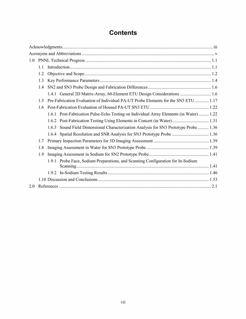
The objective of the work conducted at PNNL and reported here is to demonstrate the ability to detect a target feature, equivalent to the largest cross section of an isolated pin used within the MARICO-2 test sub-assembly, submersed in 260°C liquid sodium. Figure 1.1 illustrates the Japanese Joyo reactor fuel sub-assembly and the cross sectional dimensions of a simulated pin. In the present fiscal year (FY15), emphasis was focused on design, fabrication, and assessment of a 2D, matrix array probe, operated in TRL mode, and comprised of 10×3(×2) arrays. A performance characterization activity was conducted and testing of this immersible PA-UT probe in water was performed. In addition, a performance demonstration protocol was developed and implemented for in-sodium target detection trials using the FY14 1D linear phased-array probe ETU known as SN2. These tests were conducted at 260°C, and the results are documented in this report.

1.4

Figure 1.1. Side-view Schematic, Illustrating the Japanese Joyo Reactor Fuel Sub-assembly and the

Associated Cross-Sectional Dimensions of an Isolated Pin (simulated here), within the MARICO-2 Test Sub-assembly

The scope of the PNNL efforts conducted in FY15 includes performing an evaluation and assessment of the performance characteristics of the SN3 PA-UT matrix array probe, manufactured at PNNL. This assessment is based on probe performance in water (at room temperature). In addition, PNNL’s FY15 scope included an assessment of the 3D image quality resulting from water and in-sodium PD tests of the SN2 probe, as a function of primary inspection parameters. The PD protocol employed for these tests was documented and provided in Diaz et al. (2015), and the results of this PD are presented here. These primary inspection parameters include such factors as inspection time, spatial sampling frequency, sensor-to-target distance, sodium temperature, thermal cycling, etc. The work described here, associated with the SN3 matrix array probe, is based on technical evaluations and tests obtained at two different stages of fabrication: pre-fabrication – before the SN3 array was permanently enclosed within the sensor housing, and post-fabrication – after the SN3 array was permanently welded and enclosed within the housing.

1.3 Key Performance Parameters

This section of the report defines the key performance parameters and critical attributes that provide the criteria for assessing the performance, functionality, and effectiveness of a phased-array ultrasonic testing probe. The effort reported here is focused on analysis of data and performance metrics obtained from the 2D matrix array, PA-UT prototype probe SN3. These data are used to discuss the performance characteristics of the SN3 probe. In this section, the evaluation will not include performance of the SN3 probe in sodium, but will instead focus on the performance characteristics via direct measurements obtained prior to housing the elements, after housing the elements, and in water, at room temperature.

American Society for Testing and Materials (ASTM) E2491-13 is a standard guide for evaluating performance characteristics of phased-array ultrasonic probes (ASTM E2491-13). In addition, for PA-UT probes where single focal laws essentially fix the beam and electronic or sectorial scan modes are not employed, ASTM E1065 offers standard guidance using a ball target in an immersion test setting (ASTM E1065/E1065M-14). In FY13, PNNL reported some work in the joint technical report on USV progress with Argonne National Laboratory (ANL) that focused on obtaining data for characterization of the SN1

1.5

PA-UT probe (Braatz et al. 2013). PNNL used the key performance parameters outlined in this report, and also acquired data supporting the use of additional metrics and attributes for the prototype probes that were developed, to effectively compare performance of these ETUs. From the efforts conducted in FY13 and FY14, the following characterization tests are listed for review. Not all of these tests were conducted on the SN3 probe. During the FY15 performance testing of the SN3 ETU, it became apparent that this probe would not produce sufficient signal amplitudes to warrant further testing, and additionally, system noise became a challenge late in the evaluation process, so additional performance characterization tests were aborted. The list of tests includes:

1. Pre-fabrication pulse-echo testing on individual array elements (in water)

2. Post-fabrication pulse-echo testing on individual array elements (in water)

a. Validation of array pin connections

b. Evaluation of transmit uniformity per element (using a pinducer as the receiving probe in raster scan mode)

c. Evaluation of element-to-element cross talk (to assess inter-element coupling between neighboring elements)

d. Evaluation of selected depth focus points

e. Evaluation of selected angles (to assess how effectively the probe can skew the sound field off its 0° primary axis)

3. Post-fabrication assessment of temperature resistance and thermal cycling effects (in hot oil).

In addition to these tests, PNNL conducted post-fabrication characterization assessments aimed at quantifying a suite of additional critical attributes, including:

4. Individual voltage responses from each element after employing a standard excitation pulse, and reflected from a polished, fused silica reflector plate (conducted in pulse-echo mode, without the use of a separate pinducer for receiving signal responses)

5. Center and peak frequency responses from the fast Fourier transforms (FFTs) of individual element responses in #4 above

6. −6 dB (decibels) bandwidths (BWs) of each element, calculated from #5 above

7. Sensitivity variations (in normalized % amplitude) from element-to-element

8. Sound field dimensions (focal spot size) at −6 dB and −12 dB points at a nominal distance from the face of the probe in water, using a pinducer receiving probe

9. Spatial resolution testing using raster scanning of the probe and employing flat reflectors with various spacings to evaluate array resolution performance in water

10. Evaluation of SNR from both pre-fabrication testing of the individual elements and post-fabrication tests.

With the analyses of the data obtained from many of these performance characterization tests, PNNL was able to quantify key performance parameters used to assess the viability of implementing the SN3 ETU in sodium. In particular, sound field dimensions (spot size), resolution capabilities, SNR, frequency response, and BW characteristics constitute the suite of critical attributes used to evaluate this probe and to support any future decisions regarding viability for continued optimization in FY16. Examples of test data and results from these performance assessments are provided in Sections 1.5 and 1.6, and the conclusions obtained from the performance evaluations of both ETU probes are discussed in Section 1.10.

1.6

1.4 SN2 and SN3 Probe Design and Fabrication Differences

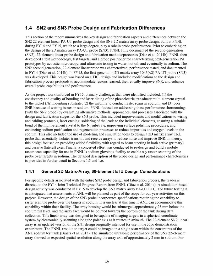
This section of the report summarizes the key design and fabrication aspects and differences between the SN2 22-element linear PA-UT probe design and the SN3 2D matrix array probe design, built at PNNL during FY14 and FY15, which to a large degree, play a role in probe performance. Prior to embarking on the design of the 2D matrix array PA-UT probe (SN3), PNNL fully documented the second-generation (SN2), 22-element linear probe design and fabrication methods/processes (Diaz et al. 2014b). PNNL then developed a test methodology, test targets, and a probe positioner for characterizing next-generation PA prototypes by acoustic microscopy, and ultrasonic testing in water, hot oil, and eventually in sodium. The SN2 second generation, 22-element linear probe was characterized, performance tested, and documented in FY14 (Diaz et al. 2014b). In FY15, the first-generation 2D matrix array 10×3(×2) PA-UT probe (SN3) was developed. This design was based on a TRL design and included modifications to the design and fabrication process protocols to accommodate lessons learned, theoretically improve SNR, and enhance overall probe capabilities and performance.

As the project work unfolded in FY15, primary challenges that were identified included: (1) the consistency and quality of bonding and laser-dicing of the piezoelectric transducer multi-element crystal to the nickel (Ni) mounting substrate; (2) the inability to conduct raster scans in sodium; and (3) poor SNR because of wetting issues in sodium. PNNL focused on addressing these performance shortcomings (with the SN2 probe) by evaluating alternative methods, approaches, and processes associated with the design and fabrication stages for the SN3 probe. This included improvements and modifications to wiring and cabling protocols, laser etching, soldering of the leads to the individual elements, ensuring a suitable bond of the multi-element crystal to the Ni substrate, improving surface polishing procedures, and enhancing sodium purification and regeneration processes to reduce impurities and oxygen levels in the sodium. This also included the use of modeling and simulation tools to design a 2D matrix array TRL probe that essentially isolates transmit and receive arrays to reduce noise and improve SNR. In theory, this design focused on providing added flexibility with regard to beam steering in both active (primary) and passive (lateral) axes. Finally, a concerted effort was conducted to re-design and build a mobile raster-scan capability for use in PNNL’s sodium glovebox facility to enable x-y raster scanning of the probe over targets in sodium. The detailed description of the probe design and performance characteristics is provided in further detail in Sections 1.5 and 1.6.

1.4.1 General 2D Matrix-Array, 60-Element ETU Design Considerations

For specific details associated with the entire SN2 probe design and fabrication process, the reader is directed to the FY14 Joint Technical Progress Report from PNNL (Diaz et al. 2014a). A simulation-based design activity was conducted in FY15 to develop the SN3 matrix array PA-UT ETU. For future testing it is anticipated that assessments at ANL will be planned as part of the scope for out-year activities on this project. However, the design of the SN3 probe incorporates specifications requiring the capability to raster scan the probe over the targets in sodium. It is unclear at this time if ANL can accommodate this capability within their facility. The array housing would be submerged approximately 25 mm below the sodium fill level, and the array face would be pointed towards the bottom of the tank during data collection. This linear array was designed to be capable of imaging targets in a spherical coordinate system by electronically scanning along the polar axis as it rotates in azimuth. The 22-element SN2 linear array is an updated version of the SN1 design originally intended for use in the Joyo demonstration experiment. The PNNL resolution target could be imaged in a single scan within the constraints of the ANL sodium test tank (Braatz et al. 2013). The simulated ultrasonic performance of the SN2 22-element array showed an expected spatial resolution along the array axis of approximately 2 mm in sodium. For

1.7

the comparative assessment of the SN2 and SN3 probes provided in this TLR, spatial resolution tests in water are used to determine and assess the performance differences.

In FY15, PNNL worked to improve the probe design in order to enhance sound field propagation and ultimately increase image resolution in sodium. The key array design parameters included moving from a 1D linear-array configuration to a 2D matrix-array, TRL configuration. This change in design and technical direction was aimed at improving resolution and sensitivity, increasing the volume of examination (via enhanced beam control and steering in primary and secondary axes), and improving signal fidelity and SNR through isolation of the transmit and receive array elements. In addition, the ability to improve sound field focal dimensions and the capability of invoking a raster-scan modality for data acquisition were viewed as positive enhancements that would lead to improved target detection and characterization performance in sodium.

1.4.1.1 SN2 and SN3 ETU Mechanical Design Differences

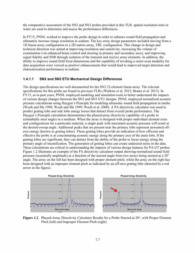
The design specifications are well documented for the SN2 22-element linear-array. The relevant specifications for this probe are found in previous TLRs (Watkins et al. 2012; Braatz et al. 2013). In FY15, as in past years, PNNL employed modeling and simulation tools to better understand the impacts of various design changes between the SN2 and SN3 ETU designs. PNNL employed normalized acoustic pressure calculations using Huygen’s Principle for modeling ultrasonic sound field propagation in media (Wooh and Shi 1998; Wooh and Shi 1999; Wooh et al. 2000). A PA directivity calculator was used to predict grating lobe and side lobe energy losses that detract from overall probe performance. The Huygen’s Principle calculation demonstrates the phased-array directivity capability of a probe to azimuthally steer angles in a medium. When the array is designed with proper individual element sizes and configurations for a particular material, a single peak with maximum acoustic pressure will result at the desired sweep angle. Additional peaks that are present near the primary lobe represent unwanted off-axis energy (known as grating lobes). These grating lobes provide an indication of how efficient and effective the probe is at concentrating acoustic energy along the primary axis of the main lobe. If the grating lobes are significant, they can detract from the ability of the probe to focus energy along the primary angle of insonification. The generation of grating lobes can create undesired noise in the data. These calculations are critical in understanding the impacts of various design features for PA-UT probes. Figure 1.2 illustrates an example of the PA directivity calculator output showing normalized sound field pressure (essentially amplitude) as a function of the steered angle from two arrays being steered at a 20° angle. The array on the left has been designed with proper element pitch, while the array on the right has been designed with an improper element pitch as indicated by an off-axis grating lobe (denoted by a red arrow in the figure).

Figure 1.2. Phased-Array Directivity Calculator Results for a Probe Steered at 20°, with Proper Element

Pitch (left) and Improper Element Pitch (right)

1.8

In addition to this tool, PNNL also employed Zetec’s UltraVision software version 3, for simulating the sound fields from various 2D matrix-array TRL designs. In order to theoretically evaluate various probe design specifications and assess the impacts of these design parameters on the resultant simulated sound fields, the following design features were considered:

1. The new probe would be comprised of separate transmit and receive arrays to better isolate transmitted and received sound energy and improve SNR. This is known as the transmit-receive longitudinal configuration.

2. A decision was made to design a planar array configuration where no roof angle would be applied. This requires electronic skewing of the planar arrays, but significantly reduces the level of complexity required for fabrication and fixturing, and provides a longer depth of field.

3. A minimum element size is needed to minimize laser dicing limitations and hand soldering issues, including the potential for shorting adjacent elements and increasing mechanical cross talk with a reduced gap size.

4. Since the Tomoscan III system (the PA-UT data acquisition instrument available for use on this project) has a limited number of total channels (64), the maximum number of transmit and receive channels are 32 simultaneous transmit channels and 32 receive. This translates into a limited set of possible array configurations to maximize the working distance along the active axis. Arrays of 8×4 and 10×3 were considered here. This correlates to a minimum aperture (in the active axis) of 15.8 mm and 19.8 mm, respectively, which are fabrication constraints.

5. It was decided to maintain the frequency requirement for this probe design. Thus, the nominal operating frequency of the probe was maintained at 2.0 MHz to be consistent with previous designs and retain a wavelength in liquid sodium of 1.23 mm). This wavelength is compatible for meeting the required resolution to detect an 11 × 6 mm Joyo fuel pin.

6. A desired working distance of 75 mm was identified as optimal, but 50 mm distance was also considered. This has impact to the array length for effective scan performance in the active axis.

7. An assumption of a 50% −6 dB BW was used as an initial design consideration for these simulations. This was consistent with other probe designs in FY13 and FY14.

The PA directivity calculator was used to assess both the 8×4 and 10×3 TRL configurations. For each array configuration, various specifications were evaluated, and these included focal distance, steering angle, probe separation, primary and secondary pitch, and element dimensions and, of course, total aperture dimensions. Table 1.1 provides the various values for these design parameters for each of the array configuration scenarios that were simulated. True-depth focusing was applied at 25, 50, and 75 mm and steering angles were incremented in 1° steps. The spatial resolution for these sodium simulations was set to 0.3 × 0.3 mm.

Simulations conducted for scenarios in Case #1 indicated that the aperture size was insufficient to provide the required beam steering performance. In addition, this design would only provide a working distance of 19 mm in sodium and the required element and gap sizes for this array design were well below current fabrication capabilities involving hand-soldering techniques. Simulations of Case #2 are illustrated in Figure 1.3 and show that, with an increased aperture, the working distance of 76 mm is achievable in sodium, but the advent of significant grating lobes limit the beam steering performance of this design.

1.9

Table 1.1. Array Design Parameter Considerations for Theoretical Assessments

Case #

Focal Distance

(mm)

Steering Angle

(°)

T-R Array Separation

(mm)

Primary Pitch (mm)

Primary Element

(mm)

Secondary Pitch (mm)

Secondary Element

(mm)

Total Aperture

(mm)

1 25/50/75 0–10 5/10 1.25 1.0 1.25 1.0 9.75×4.75 2 25/50/75 0–15 5/10 2.45 2.35 2.45 2.35 19.5×19.4 3 25/50/75 0–15 5 2.0 1.8 2.0 1.8 19.8×5.8 4 25/50/75 0–15 10 2.0 1.8 2.0 1.8 19.8×5.8

Figure 1.3. (a) Simulated Sound Field (main lobe and grating lobes) Emanating from Case #2 Design

Scenario. Phased Array Directivity Calculator Results for an 8×4 TRL Matrix PA-UT Probe Steered at (b) 0° and (c) 15° in the Active Axis.

Simulated results for the scenarios in Cases #3 and #4 exhibited similar performance at the focal depths evaluated in this study. The scenarios in both cases yielded similar sound field dimensions (spot sizes) across the spectrum of focal depths and steering angles, and grating lobes were generally well below −20 dB for both cases. Because of similarities in theoretical performance, Case #4 was selected as the final design parameter set for the SN3 2D matrix-array PA-UT ETU probe. The additional 5 mm of edge-to-edge transmit-receive array separation provided additional space for manipulation and placement of array magnet wires and provided space for hand soldering of wires to individual elements. The active axis

1.10

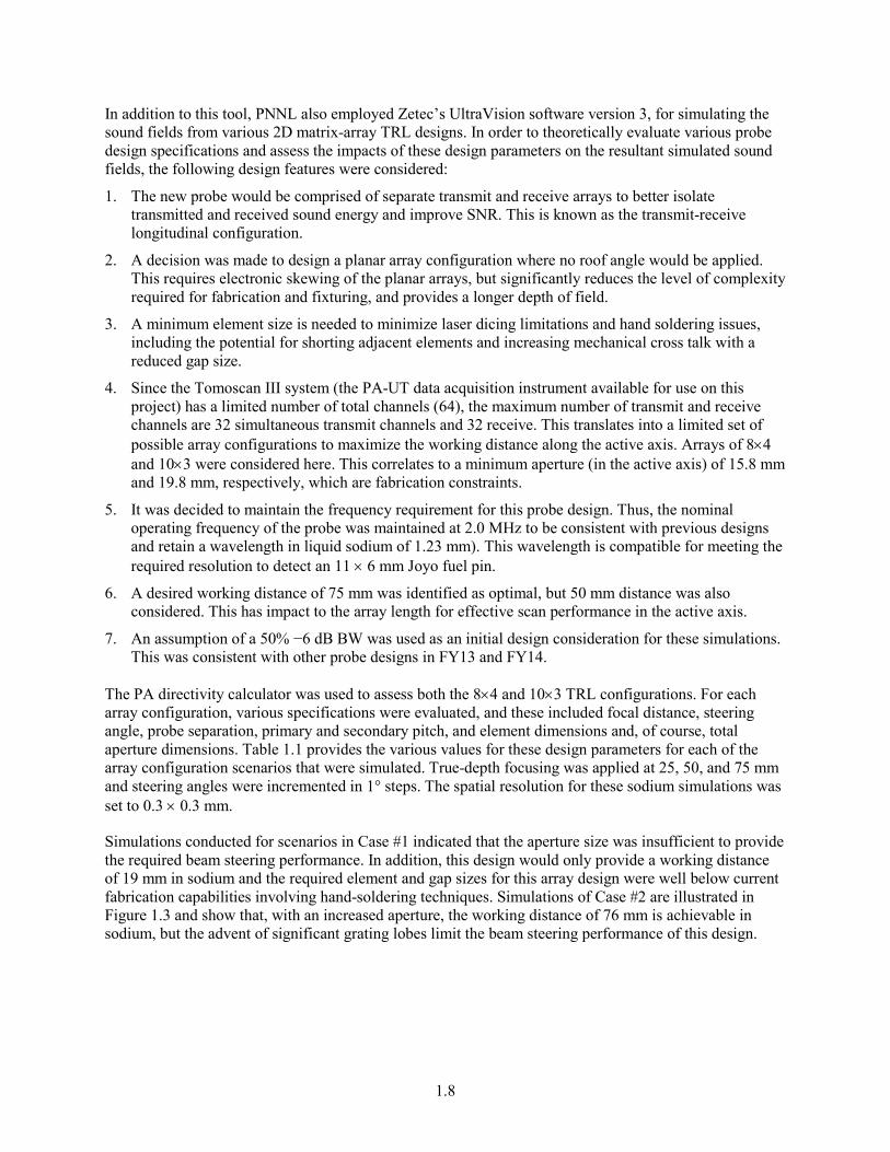
scan range of ± 12° corresponds to ± 10.5 mm of target coverage at 50 mm focal distance, while at 75 mm focal distance this target coverage region expands to ± 16 mm. Grating lobes for this case are in the −40 dB range. If the envelope is widened to include a scan range of ± 15°, this results in the generation of −20 dB grating lobes. While this would be considered the maximum extent of the scan range for this set of design parameters, the corresponding target coverage region at a 75 mm focal depth in sodium would extend to ± 20 mm. The PA directivity plots for the 10×3 matrix-array design cases are provided in Figure 1.4 for a range of active axis scan angles of up to 12°. The UltraVision-generated beam simulations for Case #4 at a 75 mm focal depth are provided in Figure 1.5.

Figure 1.4. Phased Array Directivity Calculator Results for a 10×3 TRL Matrix PA-UT Probe Steered

over a Range of Angles from 0° to 12° in the Active Axis

In Figure 1.5, at the 10° angle, a grating lobe at −40 dB is slightly noticeable to the left of the primary (main) lobe. At the 75 mm focal distance at a 0° angle, the simulated spot size dimension in the active axis was measured to be 3.71 mm and in the passive axis was measured to be 12.28 mm, with a 54 mm depth of field at the 6 dB point. These results provided information used to determine the final design parameters for the SN3 2D matrix-array PA-UT probe in FY15. The 10×3 TRL array configuration with 10 mm separation (Case #4) was the design of choice, with 2.0 mm element pitch, 1.8 mm element size and 19.8 × 5.8 mm total transmit aperture. With this design, the total number of coaxial cables and magnet wires increased from 22 to 60. Finally, the Swagelock VCR fitting was again removed from this design.

1.11

Figure 1.5. UltraVision Sound Field Simulations for a 10×3 TRL Matrix PA-UT Probe Steered over a

Range of Angles from 0° to 10° in the Active Axis at a 75 mm Focal Distance

With regard to lateral beam steering capability, the illustration in Figure 1.6 shows the simulated sound field emanating from the probe (at an angle) and skewed 10°. Lateral steering of 10° only shifts the center of the focal spot by approximately 1.5 mm at the most extreme steering angle along the active axis. The sound beam would shift more in the lateral direction if the proposed design scenarios were physically capable of steering beyond 10°, but this is not the case under the constraints identified here. Lateral sound beam steering (along the passive axis) was not evaluated in this simulation study with the 10×3 design, as steering in this direction is generally not very effective with only three elements along the passive axis. Beam steering in the lateral direction is typically more effective when significant steering in the active axis can be accomplished. The design constraints were the limiting factor in this assessment.

Figure 1.6. UltraVision Sound Field (spot) 10° Lateral Beam Steer Simulation for a 10×3 TRL Matrix

PA-UT Probe Steered at an Active Axis Angle of 10° at a 75 mm Focal Distance

1.12

1.4.1.2 SN2 and SN3 Fabrication Process Differences (Enhancements)

The fabrication process outlined previously in the FY14 Joint TLR for the SN2 22-element linear array was essentially followed for the SN3 2D matrix-array ETU. However, a few critical process modifications were introduced between the SN2 and SN3 design efforts. In particular, element isolation via an improved laser dicing process was implemented, and the transmit and receive arrays were physically sliced apart from one another to better isolate each array. Figure 1.7 shows the laser machined cup assembly for the SN3 probe. Process improvements conducted by the vendor included improved solder materials, enhanced control of solder pooling, and employed a higher process temperature. As a result of this improved process, re-poling of the elements was not required for the SN3 probe, as it was for the SN1 probe in FY13.

Figure 1.7. Laser Machined Cup Assembly for the SN3 60-Element Matrix Array PA-UT ETU

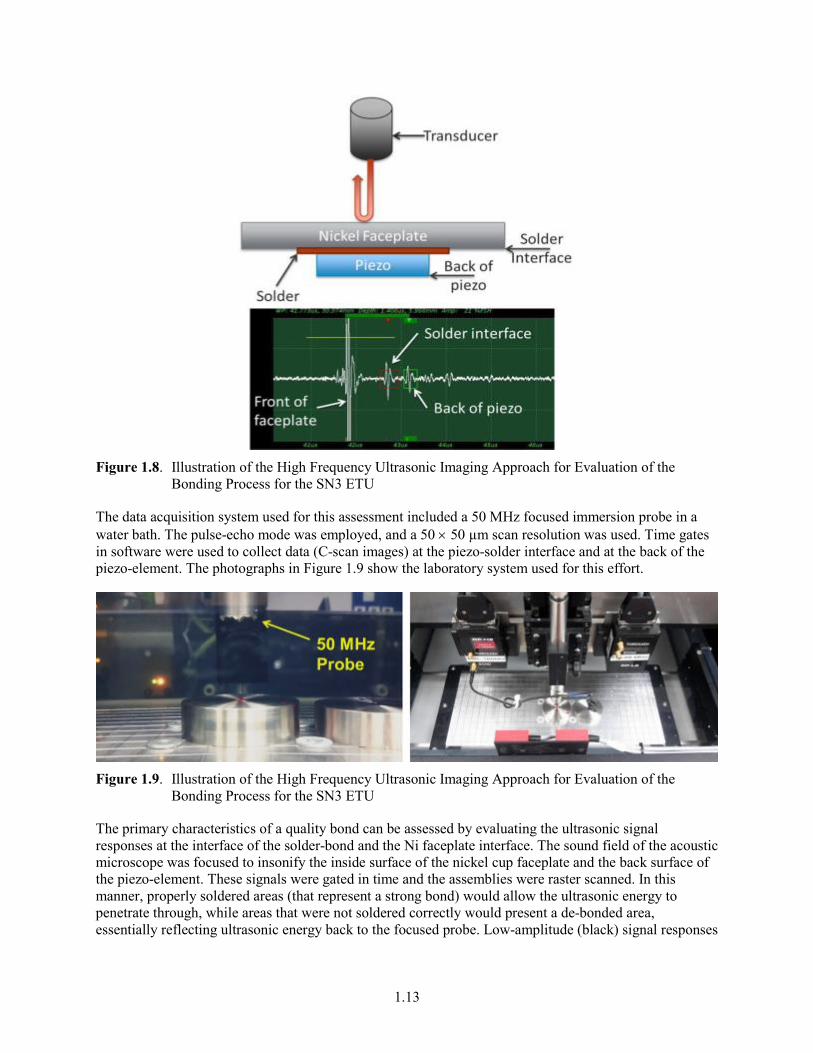
The SN3 piezo-element was bonded to the cup assembly using a solder strip in an industrial oven at a temperature of 340°C. A copper weight and associated fixture were placed on top of the piezo-element to ensure centering of the element and maintain even pressure for bonding between the element and the Ni faceplate. With the SN3 prototype, the Ni cup and faceplate were designed and fabricated as a single assembly. The faceplate thickness increased to 0.100 in. and was then subsequently machined to approximately 0.060 in. after completing the piezo-element solder/bonding process. The piezo-element was then laser diced to the specifications for a 10×3(×2) matrix array with a 10 mm separation (edge-to-edge) between transmit and receive arrays and a nominal operating frequency of 2.0 MHz. The entire PZT-5A element measured 21.6 mm × 19.8 mm (passive axis-x-active axis, respectively). Each individual element was 1.8 mm × 1.8 mm square, and each channel was laser machined to a width of 0.2 mm. The SN3 piezo-element was then evaluated for any depoling of the piezo-element after the oven-baking process. As in previous years, PNNL employed high-frequency acoustic microscopy to assess the quality and homogeneity of the high-temperature solder bond between the PZT-5A element and the Ni-200 faceplate. Figure 1.8 illustrates the technique employed to assess these bonds.

1.13

Figure 1.8. Illustration of the High Frequency Ultrasonic Imaging Approach for Evaluation of the

Bonding Process for the SN3 ETU

The data acquisition system used for this assessment included a 50 MHz focused immersion probe in a water bath. The pulse-echo mode was employed, and a 50 × 50 µm scan resolution was used. Time gates in software were used to collect data (C-scan images) at the piezo-solder interface and at the back of the piezo-element. The photographs in Figure 1.9 show the laboratory system used for this effort.

Figure 1.9. Illustration of the High Frequency Ultrasonic Imaging Approach for Evaluation of the

Bonding Process for the SN3 ETU

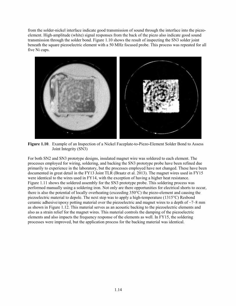
The primary characteristics of a quality bond can be assessed by evaluating the ultrasonic signal responses at the interface of the solder-bond and the Ni faceplate interface. The sound field of the acoustic microscope was focused to insonify the inside surface of the nickel cup faceplate and the back surface of the piezo-element. These signals were gated in time and the assemblies were raster scanned. In this manner, properly soldered areas (that represent a strong bond) would allow the ultrasonic energy to penetrate through, while areas that were not soldered correctly would present a de-bonded area, essentially reflecting ultrasonic energy back to the focused probe. Low-amplitude (black) signal responses

1.14

from the solder-nickel interface indicate good transmission of sound through the interface into the piezo-element. High-amplitude (white) signal responses from the back of the piezo also indicate good sound transmission through the solder bond. Figure 1.10 shows the result of inspecting the SN3 solder joint beneath the square piezoelectric element with a 50 MHz focused probe. This process was repeated for all five Ni cups.

Figure 1.10. Example of an Inspection of a Nickel Faceplate-to-Piezo-Element Solder Bond to Assess

Joint Integrity (SN3)

For both SN2 and SN3 prototype designs, insulated magnet wire was soldered to each element. The processes employed for wiring, soldering, and backing the SN3 prototype probe have been refined due primarily to experience in the laboratory, but the processes employed have not changed. These have been documented in great detail in the FY13 Joint TLR (Braatz et al. 2013). The magnet wires used in FY15 were identical to the wires used in FY14, with the exception of having a higher heat resistance. Figure 1.11 shows the soldered assembly for the SN3 prototype probe. This soldering process was performed manually using a soldering iron. Not only are there opportunities for electrical shorts to occur, there is also the potential of locally overheating (exceeding 350°C) the piezo-element and causing the piezoelectric material to depole. The next step was to apply a high-temperature (1315°C) Resbond ceramic adhesive/epoxy potting material over the piezoelectric and magnet wires to a depth of ~7–8 mm as shown in Figure 1.12. This material serves as an acoustic backing to the piezoelectric elements and also as a strain relief for the magnet wires. This material controls the damping of the piezoelectric elements and also impacts the frequency response of the elements as well. In FY15, the soldering processes were improved, but the application process for the backing material was identical.

1.15

Figure 1.11. Insulated Copper Magnet Wires Soldered to the 60-Element, Matrix Array SN3. 50%

Wired Array on the Left and Fully Wired Array on the Right.

Figure 1.12. Addition of High-Temperature Ceramic Adhesive/Epoxy Potting Material in SN3

In FY15, refinements to the manual soldering technique were applied to the fabrication process of the SN3 probe. In addition, great care was taken to physically isolate each of the individual magnet wires, by separating them during the curing process of the backing material. The design and fabrication process differences described in this section underpin some significant (anticipated) performance improvements embodied in the SN3 prototype probe, and during the pre-fabrication assessment, these improvements have been discussed here. After probe housing had been completed, the SN3 probe appears identical (from the outside) as the previous SN2 probes (built in FY14), with the exception of the connector and cabling that were streamlined for accommodating 60 wires as opposed to 22 wires. The SN3 ETU is illustrated in Figure 1.13.

1.16

Figure 1.13. Digital Photographs of the SN3 Matrix-Array ETU, Showing the Probe Housing,

Connectors, and Cabling, Prior to the Initiation of Post-Fabrication Testing and Evaluation

The magnet wire used on the 60-element SN3 array was slightly different from the previous 9- and 22-element arrays designed in previous years, to better withstand potential heating effects from the liquid sodium. The backing material used in the array cup insulated the piezo-element connections from these potential heating effects, but a decision was made to be more conservative and further protect these connections by employing a magnet wire with higher heat resistance. The only difference between the original and new magnet wire was the coating used to insulate the wire and the length of the wires. The wire gauge was identical (MWS 30 ga). The original magnet wire was rated at 140°C and the new magnet wire was rated at 240°C. Lengths were increased from 200 mm to 355 mm.

Probe cabling on previous SN1 and SN2 probe builds were fabricated with high-temperature coax cable that was used to connect the magnet wires to the Tomoscan III PA-UT data acquisition system. This was changed on the SN3 probe, as prior probes had fewer elements and the high-temperature coax cables could be readily fed down the extension tube and soldered on to a shorter length magnet wire. With the 60-element SN3 array, there was not enough room for both magnet wire and the high-temperature coax cable inside the extension tube, so a 64-conductor medical-grade coax cable was procured and used along with a 64-pin lemo connector. A lemo plug connector was mated to the extension tube and a receptacle connector was inserted on the cable assembly. This configuration provided a more durable and effective

1.17

configuration. The high-temperature coax cable was Type RG178B, 30 ga, Teflon-coated and had a temperature specification rating of 200°C. The medical coax cable was a Microcoax, 68-conductor, 38 ga, with a PVC jacket. For reference, the temperature at the top of the probe shaft has been previously measured to be approximately 100°C.

The SN3 probe was tested with the 64 pin medical coax cable, and initial testing results in water showed a loss of signal amplitude with the medical-grade coax cable compared to that of the high-temperature coax cable. Resistance measurements were taken on both cables, and the medical coax cable measured 16 ohms per individual coax. In contrast, the high-temperature coax cable measured 3 ohms per individual coax. Use of the medical coax cable resulted in a generally lower SNR in water tests. The rationale for changing cables was to reduce the effects of the higher impedance medical coax cable to reduce potential signal attenuation. This change resulted in an average improvement of approximately 10% in signal response amplitudes. A digital photograph of the final cabling configuration used on the SN3 ETU is provided in Figure 1.14.

Figure 1.14. Digital Photograph of the Final SN3 Matrix-Array ETU, Showing the Probe Housing, Final

Connectors, and Cabling Used in All Post-Fabrication Testing and Evaluation Activities

1.5 Pre-Fabrication Evaluation of Individual PA-UT Probe Elements for the SN3 ETU

This section describes the measurements and data obtained on the second build of the SN3 ETU PA-UT probe prior to housing the elements, but after potting of the laser etched, 60-element array within the Ni

1.18

cup. A set of pulse-echo tests were conducted on the post-potted assemblies to (1) ensure that each individual array element provides an acoustic response to a narrow square-wave electrical input signal, (2) to make a relative comparison of the amplitude responses of each element to determine if any are “weak” or “unresponsive,” and (3) to establish a baseline for the amplitude response. Weak or unresponsive elements would provide a qualitative indication of depoling occurring as a result of exceeding the piezoelectric Curie temperature of 350°C during the soldering processes. Depoling could be localized to a heat-affected zone in the vicinity of the magnet wire-to-piezoelectric solder joint, permitting the element to continue functioning, but with a weaker response. Unresponsive elements would indicate total depoling or alternatively an electrical disconnect of the magnet wire from the piezoelectric element. The tests were conducted by placing only the external, sodium-facing side of the cup assembly into a water bath with a 3 mm spacing away from a pinducer to obtain signal responses for these measurements. Each individual element was driven with a short-duration 180V square-wave pulse (250 ns) at a suitable repetition rate for data acquisition. This pulse length was chosen to optimally excite the piezoelectric elements at their fundamental design frequency of 2.0 MHz.

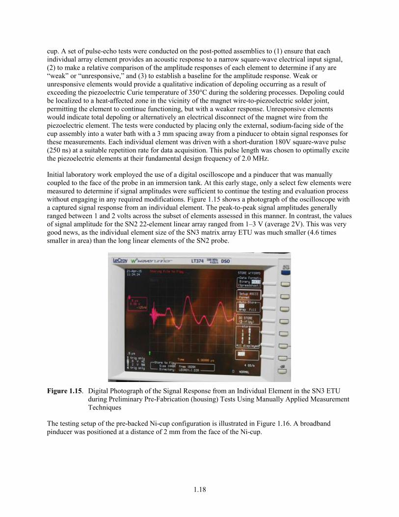
Initial laboratory work employed the use of a digital oscilloscope and a pinducer that was manually coupled to the face of the probe in an immersion tank. At this early stage, only a select few elements were measured to determine if signal amplitudes were sufficient to continue the testing and evaluation process without engaging in any required modifications. Figure 1.15 shows a photograph of the oscilloscope with a captured signal response from an individual element. The peak-to-peak signal amplitudes generally ranged between 1 and 2 volts across the subset of elements assessed in this manner. In contrast, the values of signal amplitude for the SN2 22-element linear array ranged from 1–3 V (average 2V). This was very good news, as the individual element size of the SN3 matrix array ETU was much smaller (4.6 times smaller in area) than the long linear elements of the SN2 probe.

Figure 1.15. Digital Photograph of the Signal Response from an Individual Element in the SN3 ETU

during Preliminary Pre-Fabrication (housing) Tests Using Manually Applied Measurement Techniques

The testing setup of the pre-backed Ni-cup configuration is illustrated in Figure 1.16. A broadband pinducer was positioned at a distance of 2 mm from the face of the Ni-cup.

1.19

Figure 1.16. (a) Automated X-Y Raster Scanning Platform and Immersion Tank Used for Pre- and Post-

Backed Element Testing of the SN3 ETU Probe. (b) Magnified View of the Pre-Backed Ni-Cup with Individual Magnet Wires Accessible for Element-by-Element Tests.

Figures 1.17 and 1.18 show the amplitudes of the pulse-echo signal responses (at the same gain) of a single element versus time for the SN3 prototype probe, in both pre-backed and post-backed Ni housing conditions, respectively. In addition, the FFTs of these signals are provided as well.

Figure 1.17. (a) A-scan (amplitude versus time) Signal Response from Element #8 of the SN3 Probe

Prior to Backing. (b) Frequency Spectrum Generated from FFT of Time Windowed A-scan.

1.20

Figure 1.18. (a) A-scan (amplitude versus time) Signal Response from Element #8 of the SN3 Probe

Post-Backing. (b) Frequency Spectrum Generated from FFT of Time Windowed A-scan.

From a review of the data obtained from all 60 elements (within the time-gated window as shown in Figures 1.17 and 1.18), the individual pulse-echo signal responses from the elements of the SN3 probe (with backing) were generally reduced in amplitude (dampened) and slightly cleaner (less noisy) than those collected prior to backing. For each element, at a nominal gain setting that was not changed during data acquisition, the maximum peak-to-peak signal amplitude response was recorded. These data were analyzed and the FFT results were calculated to generate bandwidth for each element. From an analysis of these signal responses (see Figures 1.19 through 1.21), it was clearly evident that the individual BW and center frequency values for the SN3 probe were substantially higher in consistency (less variation) than those resulting from the SN2 probe in water in FY14, at this same stage of the testing and evaluation process. While raw signal amplitudes were slightly lower with the SN3 probe, this was anticipated because of the smaller element sizes between the linear and matrixed array designs.

Figure 1.19. Pre- and Post-Backed Element-by-Element Amplitude Response Variation for the SN3

ETU Probe

1.21

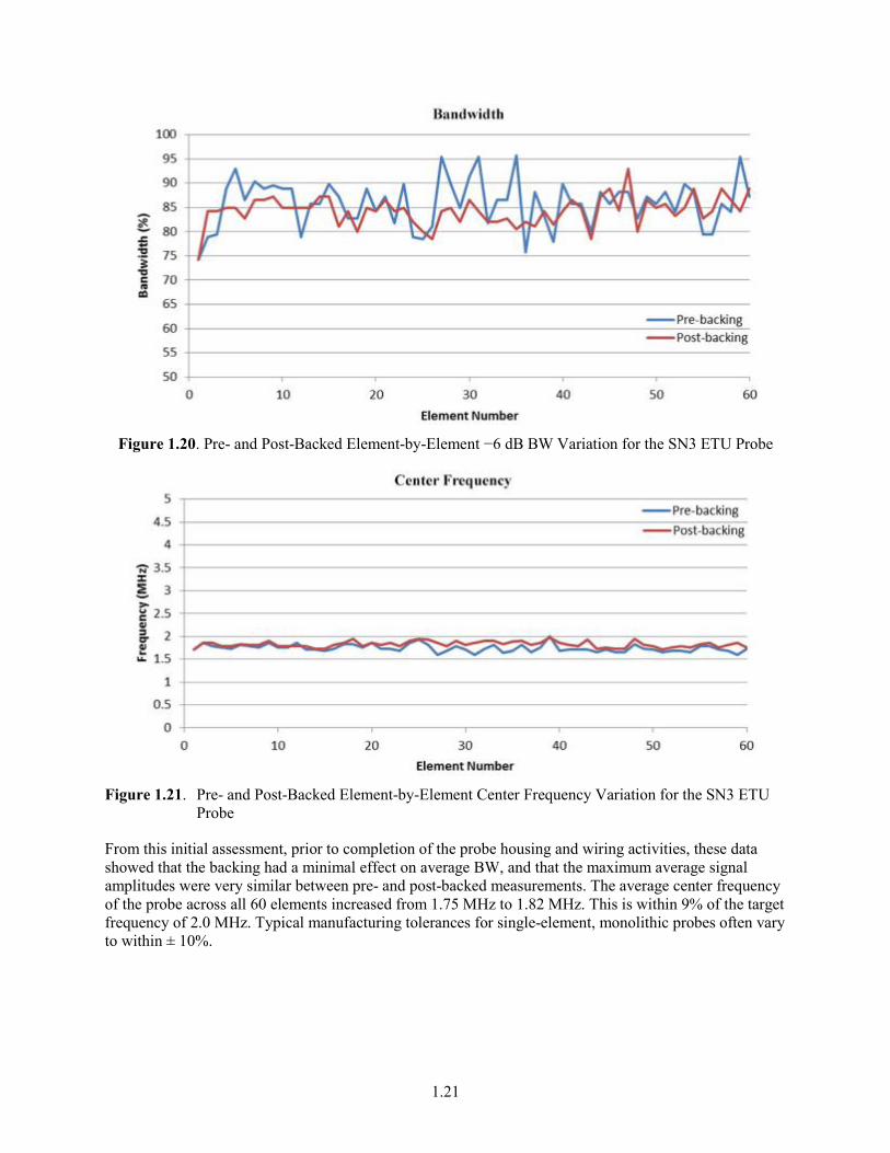
Figure 1.20. Pre- and Post-Backed Element-by-Element −6 dB BW Variation for the SN3 ETU Probe

Figure 1.21. Pre- and Post-Backed Element-by-Element Center Frequency Variation for the SN3 ETU

Probe

From this initial assessment, prior to completion of the probe housing and wiring activities, these data showed that the backing had a minimal effect on average BW, and that the maximum average signal amplitudes were very similar between pre- and post-backed measurements. The average center frequency of the probe across all 60 elements increased from 1.75 MHz to 1.82 MHz. This is within 9% of the target frequency of 2.0 MHz. Typical manufacturing tolerances for single-element, monolithic probes often vary to within ± 10%.

1.22

1.6 Post-Fabrication Evaluation of Housed PA-UT SN3 ETU

This section describes the details of performance characterization assessments and functional testing for the SN3 60-element array prototype probe, after housing had been completed. This section includes the results of post-fabrication pulse-echo testing on individual array elements (in water), for validation of array pin connections; evaluation of transmit uniformity per element (using a pinducer as the receiving probe in raster-scan mode); evaluation of element-to-element cross talk (to assess inter-element coupling between neighboring elements); evaluation of frequency response per element; evaluation of selected depth focus points; and evaluation of selected angles (to assess how effectively the probe can skew the sound field off its 0° primary axis). The center and peak frequency responses from the FFTs of these individual element responses will also be computed and evaluated here. From this information, the −6 dB BWs of each element will be calculated. The sound field dimensions (focal spot size) at −6 dB and −12 dB points at a nominal distance from the face of the probe in water, using a pinducer receiving probe, will be evaluated and contrasted. Results from spatial resolution testing using raster scanning of the probe (in pitch-catch mode) and employing elevated, flat reflectors with various spacing to evaluate array resolution performance in water, will be provided and assessed. Finally, an evaluation of SNR from both pre-fabrication testing of the individual elements and post-fabrication tests will be addressed.

1.6.1 Post-Fabrication Pulse-Echo Testing on Individual Array Elements (in Water)

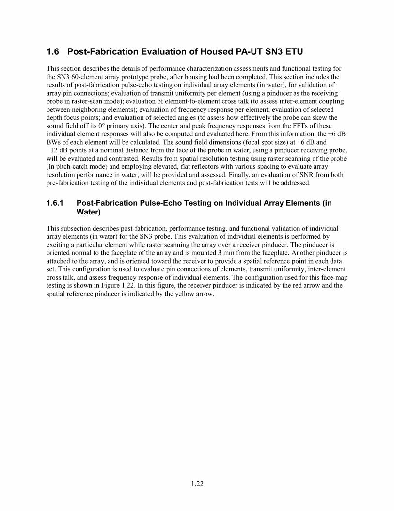
This subsection describes post-fabrication, performance testing, and functional validation of individual array elements (in water) for the SN3 probe. This evaluation of individual elements is performed by exciting a particular element while raster scanning the array over a receiver pinducer. The pinducer is oriented normal to the faceplate of the array and is mounted 3 mm from the faceplate. Another pinducer is attached to the array, and is oriented toward the receiver to provide a spatial reference point in each data set. This configuration is used to evaluate pin connections of elements, transmit uniformity, inter-element cross talk, and assess frequency response of individual elements. The configuration used for this face-map testing is shown in Figure 1.22. In this figure, the receiver pinducer is indicated by the red arrow and the spatial reference pinducer is indicated by the yellow arrow.

1.23

Figure 1.22. Facemap Assessment of Individual Elements in Water

1.6.1.1 Validation of Array Pin Connections

Centering over the fiducial pinducer (0 point) with a standoff of 3 mm (0.11 in.), raster scans were executed along the primary and secondary axis of the array where only a single element was active (0-ns delay) during a given scan. The raster scans were spatially encoded with a resolution of 0.5 mm (0.02 in.) for a scan length of 80 mm (3.1 in.) and an index length of 60 mm (2.3 in.). Each element was individually assessed for position location along the primary and secondary axis of the array and re-ordered at the Lemo connection point if necessary. In order to evaluate all elements of the array, the receiver elements were pulsed similarly to the transmitting elements. Figure 1.23 shows the UltraVision reconstruction of the raster scan of element #1 from the SN3 prototype probe. The B-scan side view (left) is along the primary axis (blue axis) and the time-gated C-scan (top) view is on the right. The purple axis (in the left image) is the time or ultrasound axis. The response from element #1 is indicated by the red arrows in the figure. For reference, the fiducial pinducer response is circled in red and appears later in time. The purpose of the fiducial is to provide a physical spatial reference point. The positional information from each element was recorded to verify that each element was wired in accordance with the element numbering produced by the UltraVision Phased-Array Calculator. The SN3 TRL array was found to have 59 of the 60 elements operational at the time these data were taken.

1.24

Figure 1.23. Raster Scan of Element #1 for the SN3 Prototype Probe. Red arrows point to element 1

response; red circle indicates the fiducial response.

1.6.1.2 Evaluation of Transmit Uniformity per Element

The previously collected raster data sets used for the validation of the array pin connections were also used to evaluate the transmit uniformity for each element. In addition, data were acquired with all elements active simultaneously with a 0 ns delay. Each element was imaged both individually as well as in concert.

Figure 1.24 shows the UltraVision reconstruction of the raster scan of element #14 (as an example) from the SN3 prototype probe using cutoff for the dynamic range. The raster scan side view (left) is along the primary axis (blue axis) and the time-gated C-scan (top) view is on the right. The purple axis (in the left image) is the time or ultrasound axis. The response from element #14 is indicated by the red arrows in the figure. Here it is shown that the element length in the active axis is 2.0 mm (0.08 in.) and 2.5 mm (0.09 in.) in the passive axis. This corresponds well with the 1.8 × 1.8 mm as-built size of the elements. Similarly, element #31 is shown in Figure 1.25, also using no dynamic range cutoff. Element #31 is an example that illustrates an over-active element where only one element is pulsed but a significant number of adjacent elements are electrically excited. In this case, the active area of the element was measured to be 5.5 × 16.0 mm, which is similar to the active area when pulsing one half of the array. This would most likely be caused by poor isolation between elements (physical or electrical) or improper element firing with the data acquisition system. This effect is present on only four excitation channels (33, 38, 40, and 53) and is not reciprocated among elements, which indicates that the cause is not related to physical/ electrical isolation but rather a pulsing issue with the data acquisition system.

1.25

Figure 1.24. Raster Scan of Element #14 for the SN3 Prototype Probe

Figure 1.25. Raster Scan of Element #31 (for the SN3 prototype probe) Showing an Over-Active

Element

Besides the nonfunctional element #18, no dead zones were identified in this evaluation for the SN3 probe; however, it is important to note that the raster scan resolution of 0.5 × 1.0 mm (002 × 0.04 in.) reduces the ability to measure amplitude variations across the small element size of 1.8 × 1.8 mm (0.07 × 0.07 in.). File size limitations imposed by the Tomoscan III data acquisition system prevented the acquisition of higher resolution data sets.

Overall, sufficient activity of all elements of the SN3 probe is shown in Figure 1.26 where the transmit side of the array is shown on top and the receive side is shown on the bottom. In this figure, the C-scan (top) view is shown on the right and B-scan (side) view is on the left. Here, all of the elements on one side of the array are pulsing simultaneously (with a delay of 0 ns between them) and the pinducer is raster scanned over the entire aperture of the array.

1.26

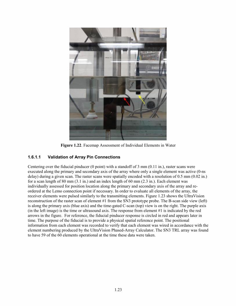
Figure 1.26. Raster Scan of Transmit and Receive Elements Pulsed at 0 ns Delay. Transmit elements are

shown above and receive elements below.

Exciting all elements of the array with no delays allows the probes to be treated as a single-element conventional array. While doing this, a pinducer was raster scanned under the array to map the signal responses and essentially capture hot/cold spots of the array in the X-Y plane under the probe at a specified distance from the probe face in water.

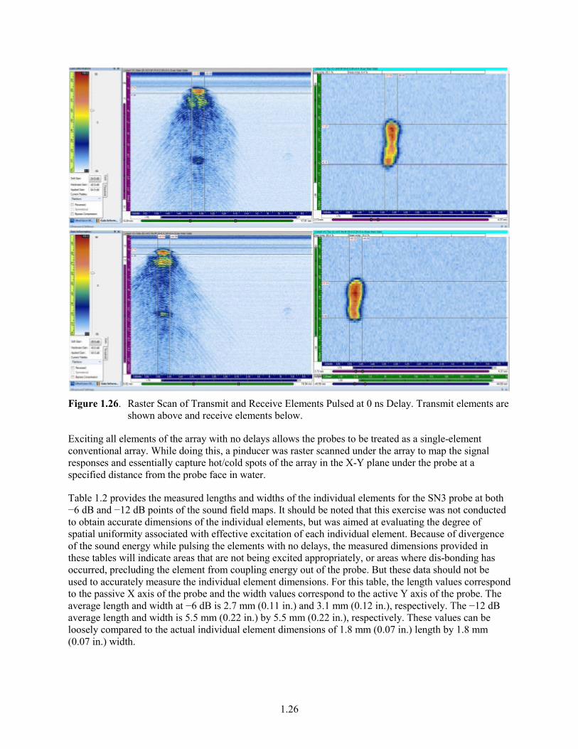
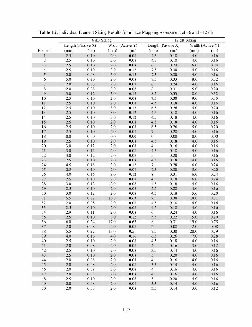
Table 1.2 provides the measured lengths and widths of the individual elements for the SN3 probe at both −6 dB and −12 dB points of the sound field maps. It should be noted that this exercise was not conducted to obtain accurate dimensions of the individual elements, but was aimed at evaluating the degree of spatial uniformity associated with effective excitation of each individual element. Because of divergence of the sound energy while pulsing the elements with no delays, the measured dimensions provided in these tables will indicate areas that are not being excited appropriately, or areas where dis-bonding has occurred, precluding the element from coupling energy out of the probe. But these data should not be used to accurately measure the individual element dimensions. For this table, the length values correspond to the passive X axis of the probe and the width values correspond to the active Y axis of the probe. The average length and width at −6 dB is 2.7 mm (0.11 in.) and 3.1 mm (0.12 in.), respectively. The −12 dB average length and width is 5.5 mm (0.22 in.) by 5.5 mm (0.22 in.), respectively. These values can be loosely compared to the actual individual element dimensions of 1.8 mm (0.07 in.) length by 1.8 mm (0.07 in.) width.

1.27

Table 1.2. Individual Element Sizing Results from Face Mapping Assessment at −6 and −12 dB

Element

−6 dB Sizing −12 dB Sizing Length (Passive X) Width (Active Y) Length (Passive X) Width (Active Y) (mm) (in.) (mm) (in.) (mm) (in.) (mm) (in.)

1 2.5 0.10 2.0 0.08 4.5 0.18 4.0 0.16 2 2.5 0.10 2.0 0.08 4.5 0.18 4.0 0.16 3 2.5 0.10 2.0 0.08 6 0.24 6.0 0.24 4 2.5 0.10 3.0 0.12 7.5 0.30 4.0 0.16 5 2.0 0.08 3.0 0.12 7.5 0.30 4.0 0.16 6 5.0 0.20 2.0 0.08 8.5 0.33 8.0 0.32 7 2.0 0.08 2.0 0.08 6 0.24 4.0 0.16 8 2.0 0.08 2.0 0.08 8 0.31 5.0 0.20 9 3.0 0.12 3.0 0.12 8.5 0.33 8.0 0.32

10 2.5 0.10 2.0 0.08 7.5 0.30 9.0 0.35 11 2.5 0.10 2.0 0.08 4.5 0.18 4.0 0.16 12 2.5 0.10 3.0 0.12 6.5 0.26 5.0 0.20 13 2.5 0.10 3.0 0.12 4.5 0.18 4.0 0.16 14 2.5 0.10 3.0 0.12 4.5 0.18 4.0 0.16 15 2.5 0.10 2.0 0.08 4.5 0.18 4.0 0.16 16 2.5 0.10 2.0 0.08 6.5 0.26 5.0 0.20 17 2.5 0.10 2.0 0.08 7 0.28 4.0 0.16 18 0.0 0.00 0.0 0.00 0 0.00 0.0 0.00 19 2.5 0.10 2.0 0.08 4.5 0.18 4.0 0.16 20 3.0 0.12 2.0 0.08 4 0.16 4.0 0.16 21 3.0 0.12 2.0 0.08 4.5 0.18 4.0 0.16 22 3.0 0.12 2.0 0.08 5 0.20 4.0 0.16 23 2.5 0.10 2.0 0.08 4.5 0.18 4.0 0.16 24 4.5 0.18 3.0 0.12 7 0.28 6.0 0.24 25 2.5 0.10 2.0 0.08 7.5 0.30 5.0 0.20 26 4.0 0.16 3.0 0.12 8 0.31 6.0 0.24 27 2.5 0.10 2.0 0.08 4.5 0.18 6.0 0.24 28 3.0 0.12 2.0 0.08 4.5 0.18 4.0 0.16 29 2.5 0.10 2.0 0.08 5.5 0.22 4.0 0.16 30 3.0 0.12 2.0 0.08 4.5 0.18 5.0 0.20 31 5.5 0.22 16.0 0.63 7.5 0.30 18.0 0.71 32 2.0 0.08 2.0 0.08 4.5 0.18 4.0 0.16 33 2.5 0.10 2.0 0.08 4.5 0.18 4.0 0.16 34 2.9 0.11 2.0 0.08 6 0.24 4.0 0.16 35 2.5 0.10 3.0 0.12 5.5 0.22 5.0 0.20 36 6.0 0.24 17.0 0.67 8 0.31 19.0 0.75 37 2.0 0.08 2.0 0.08 2 0.08 2.0 0.08 38 5.5 0.22 13.0 0.51 7.5 0.30 20.0 0.79 39 4.0 0.16 4.0 0.16 6.5 0.26 7.0 0.28 40 2.5 0.10 2.0 0.08 4.5 0.18 4.0 0.16 41 2.0 0.08 2.0 0.08 4 0.16 3.0 0.12 42 2.5 0.10 2.0 0.08 3.5 0.14 4.0 0.16 43 2.5 0.10 2.0 0.08 5 0.20 4.0 0.16 44 2.0 0.08 2.0 0.08 4 0.16 4.0 0.16 45 2.0 0.08 2.0 0.08 3.5 0.14 4.0 0.16 46 2.0 0.08 2.0 0.08 4 0.16 4.0 0.16 47 2.0 0.08 2.0 0.08 4 0.16 4.0 0.16 48 2.5 0.10 2.0 0.08 5 0.20 4.0 0.16 49 2.0 0.08 2.0 0.08 3.5 0.14 4.0 0.16 50 2.0 0.08 2.0 0.08 3.5 0.14 3.0 0.12

1.28

Element

−6 dB Sizing −12 dB Sizing Length (Passive X) Width (Active Y) Length (Passive X) Width (Active Y) (mm) (in.) (mm) (in.) (mm) (in.) (mm) (in.)

51 6.0 0.24 17.0 0.67 7.5 0.30 20.0 0.79 52 2.0 0.08 2.0 0.08 3.5 0.14 4.0 0.16 53 2.0 0.08 2.0 0.08 3.5 0.14 4.0 0.16 54 2.0 0.08 2.0 0.08 3.5 0.14 4.0 0.16 55 2.0 0.08 2.0 0.08 3.5 0.14 4.0 0.16 56 2.5 0.10 2.0 0.08 9 0.35 7.0 0.28 57 2.0 0.08 2.0 0.08 8.5 0.33 4.0 0.16 58 2.5 0.10 2.0 0.08 6.5 0.26 4.0 0.16 59 3.0 0.12 2.0 0.08 8 0.31 6.0 0.24 60 2.0 0.08 2.0 0.08 8.5 0.33 5.0 0.20

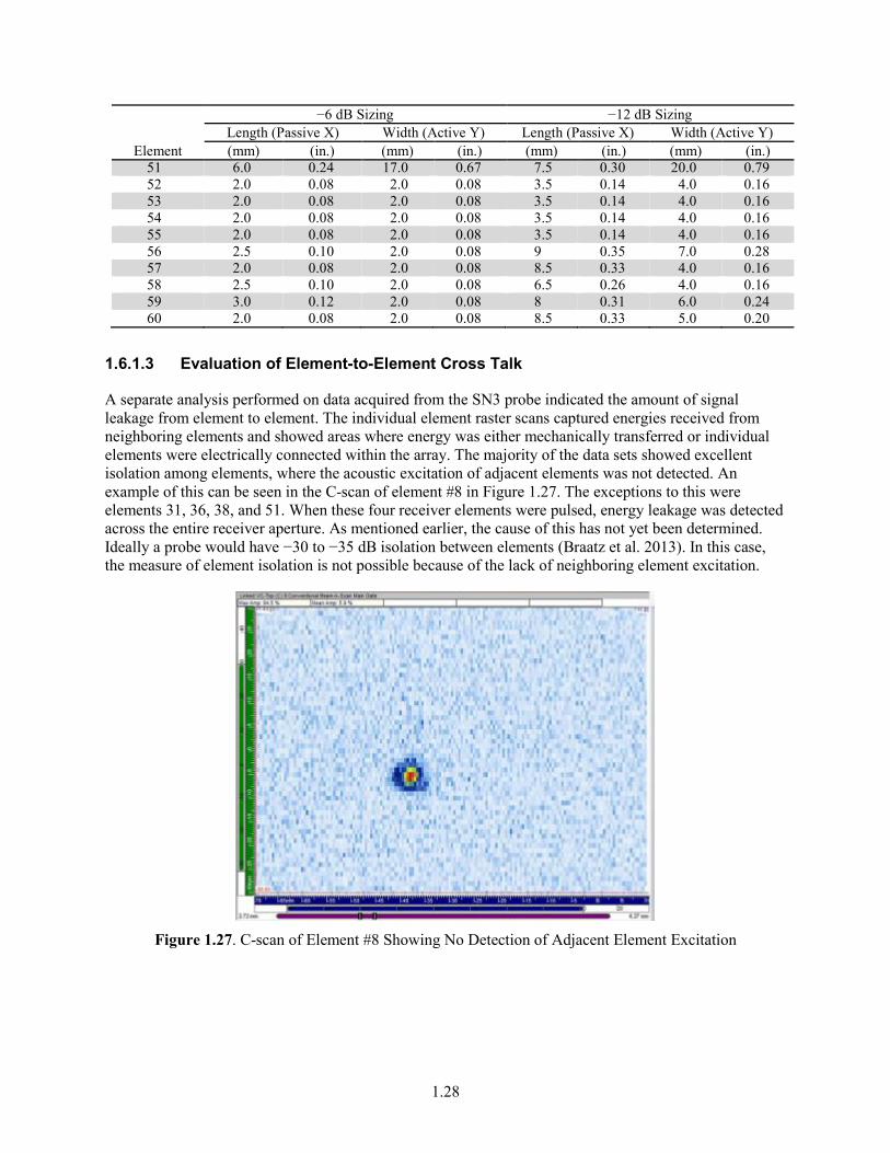
1.6.1.3 Evaluation of Element-to-Element Cross Talk

A separate analysis performed on data acquired from the SN3 probe indicated the amount of signal leakage from element to element. The individual element raster scans captured energies received from neighboring elements and showed areas where energy was either mechanically transferred or individual elements were electrically connected within the array. The majority of the data sets showed excellent isolation among elements, where the acoustic excitation of adjacent elements was not detected. An example of this can be seen in the C-scan of element #8 in Figure 1.27. The exceptions to this were elements 31, 36, 38, and 51. When these four receiver elements were pulsed, energy leakage was detected across the entire receiver aperture. As mentioned earlier, the cause of this has not yet been determined. Ideally a probe would have −30 to −35 dB isolation between elements (Braatz et al. 2013). In this case, the measure of element isolation is not possible because of the lack of neighboring element excitation.

Figure 1.27. C-scan of Element #8 Showing No Detection of Adjacent Element Excitation

1.29

1.6.1.4 Individual Element Frequency Response Analysis, and Bandwidth Calculations

This subsection describes the subsequent analysis performed on face-map data collected for each element to determine frequency response and bandwidth information. The analysis was conducted by evaluating the first arrival peak response from each element after employing a standard excitation pulse, and capturing the transmitted waveform with a pinducer as described earlier. Data were analyzed in both the time and frequency domains for each element. An example of the analysis window is shown in Figure 1.28. In this figure, the C-scan, B-scan, and D-scan views of the element response are shown along with the radio frequency (rf) waveform associated with the red reference cursors. A standard time-window was used to capture the first arrival portion of the rf-waveform response (sampling a minimum of 1½ cycles), and each individual FFT was then computed (shown center-left in Figure 1.28).

Figure 1.28. Element #11 Analysis Window for Frequency Response and Bandwidth Evaluation

From the FFTs, peak, and center frequencies were documented and the 6 dB magnitude and frequency points (both upper and lower points) were recorded as per the guidance in ASTM E-1065. Bandwidth calculations were made and are presented in Table 1.3. The average center frequency, peak frequency, and bandwidth were 1.66 MHz, 1.83 MHz, and 165%, respectively. The frequency response values are generally in agreement with the frequency response values of previously built SN1 and SN2 arrays using PZT-5A with a nickel faceplate.

1.30

Table 1.3. Element-by-Element Data and Calculations Resulting from the Frequency Response Analysis of Signal Responses from the SN3 Prototype Probe, Captured from Immersion Testing in Water Using a Pinducer as the Receiver

Element #

Center Frequency

(MHz) BW (%)

Peak Frequency

(MHz) Element

#

Center Frequency

(MHz) BW (%)

Peak Frequency

(MHz)

1 1.54 200.00 1.83 31 1.98 106.2 2 2 1.83 104.00 1.81 32 1.54 200 1.86 3 1.83 152.00 2.00 33 1.66 176.5 2 4 1.61 200.0 2 34 1.51 200 1.86 5 1.59 181.5 0.52 35 1.78 150.7 2 6 1.66 170.6 1.9 36 2.03 108.4 1.95 7 1.64 1.88 2 37 1.51 200 1.81 8 1.88 142.9 2 38 2.03 103.6 1.9 9 1.71 182.9 2 39 1.76 155.6 1.86 10 1.83 114.7 1.86 40 1.59 175.4 1.86 11 1.59 200 2 41 1.51 200 1.81 12 1.68 147.8 1.81 42 1.54 200 1.81 13 1.54 200 1.86 43 1.86 136.8 2 14 1.56 200 2 44 1.51 200 1.9 15 1.56 200 1.86 45 1.73 160.6 1.9 16 1.56 200 1.9 46 1.83 141.3 2 17 1.68 200 2 47 1.61 187.9 1.9 18 0 0 0 48 1.68 165.2 1.9 19 1.73 177.5 2 49 1.54 200 1.9 20 1.81 162.2 2 50 1.54 200 1.9 21 1.59 200 1.86 51 2.03 103.6 2.05 22 1.59 200 1.86 52 1.54 193.7 1.9 23 1.78 172.6 0.44 53 1.56 200 1.86 24 1.64 200 2 54 1.71 165.7 1.9 25 1.59 200 2 55 1.86 136.8 2 26 1.73 171.8 2 56 1.81 129.7 1.86 27 1.71 171.4 2 57 1.81 135.1 1.95 28 1.61 200 2 58 1.76 144.4 1.86 29 1.64 200 2 59 1.81 140.5 0.68 30 1.81 156.8 2 60 1.54 200 1.86

1.31

1.6.2 Post-Fabrication Testing Using Elements in Concert (in Water)

This subsection describes post-fabrication, performance testing, and functional validation of the SN3 array while using the transmitting elements in concert. This evaluation will assess the probe ability to form the sound field at specified depths and azimuthal angles in water. These evaluations were performed in similar manner to the setup used in Section 1.6.1. Unlike the individual element assessment, the receiver pinducer was not located near the faceplate of the array. Instead, the pinducer was held at a specified distance from the SN3 array for each assessment. Proper formation of the sound field at specified depths within the working distance of the array design is critical to probe performance. The performance results in these evaluations were used to determine viability of further testing.

1.6.2.1 Evaluation of Selected Depth Focus Points

The UltraVision 1.2R4 software suite was used to generate specific delay laws for the SN3 array, such that target depth focuses of 25, 50, and 75 mm (1.0, 2.0, and 3.0 in.) at 0° (azimuthal) could be achieved. The nanosecond delays are precisely timed so that the contribution from each individual element can constructively interfere with the other elements, producing a sound beam maximum at a particular depth. The reception pinducer was positioned at the depth of the focal plane and raster scanned. The raster scans were spatially encoded with a resolution of 0.5 mm (0.02 in.) in the scan direction for a scan length of 80 mm (3.1 in.) and 0.5 mm (0.02 in.) resolution in the index axis for a length of 60 mm (2.4 in.). Figures 1.29 and 1.30 show the focused beam at 0° for both 50 and 75 mm focal depths, respectively. In these figures, the top image shows the C-scan (top) view clipped at −12 dB and the lower image shows the C-scan (top) view clipped at −6 dB. Table 1.4 provides the dimensional data associated with the active and passive sound field dimensions for both the FY14 22-element linear probe and the SN3 probe as a function of focal depth. The spot sizes of the linear array are included for reference to previous performance of linear array designs.

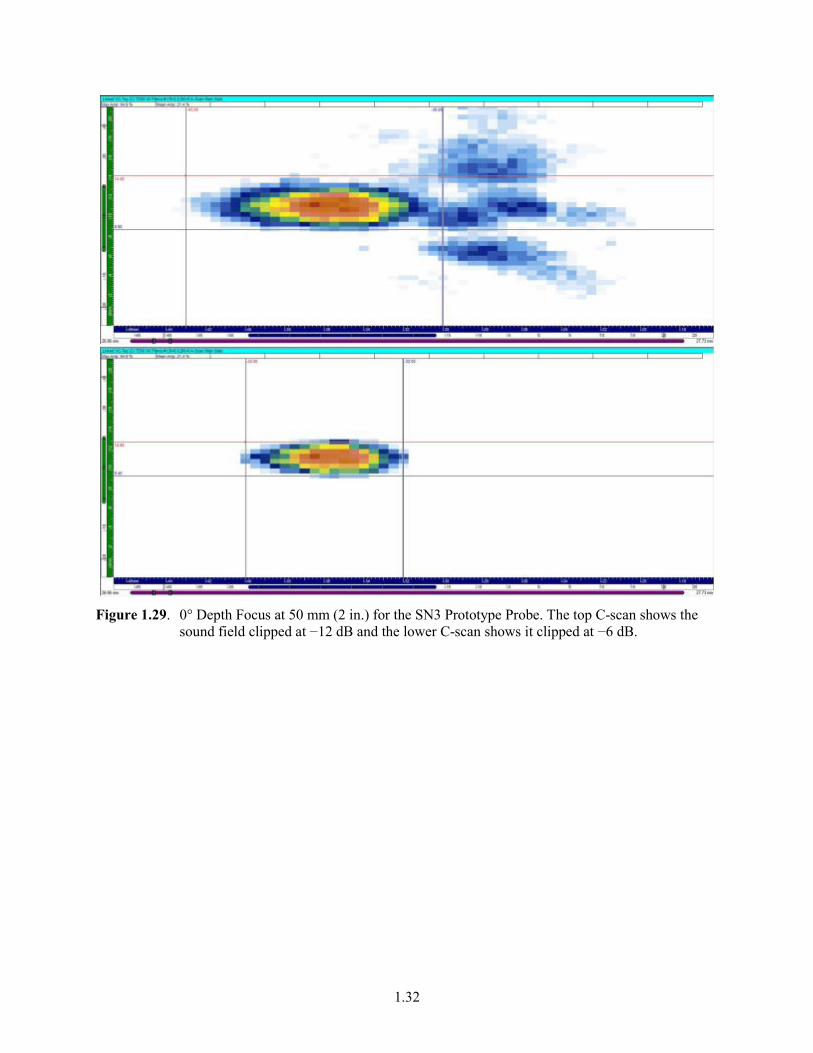
1.32

Figure 1.29. 0° Depth Focus at 50 mm (2 in.) for the SN3 Prototype Probe. The top C-scan shows the

sound field clipped at −12 dB and the lower C-scan shows it clipped at −6 dB.

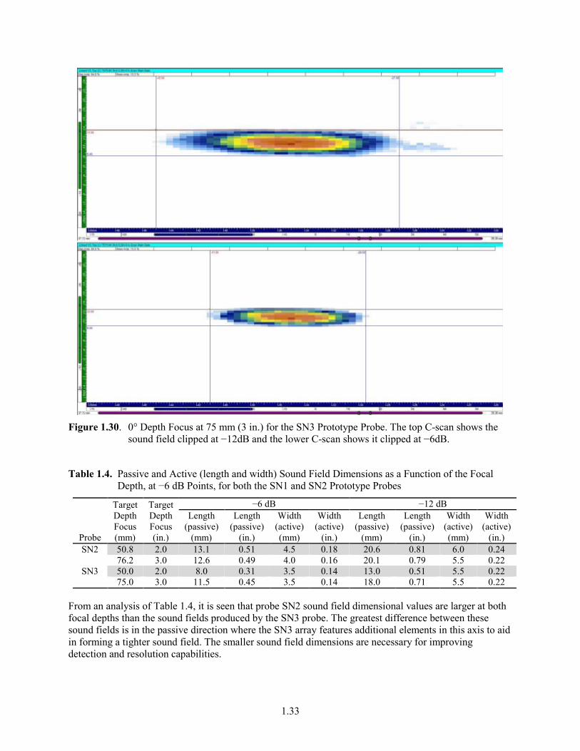
1.33

Figure 1.30. 0° Depth Focus at 75 mm (3 in.) for the SN3 Prototype Probe. The top C-scan shows the

sound field clipped at −12dB and the lower C-scan shows it clipped at −6dB.

Table 1.4. Passive and Active (length and width) Sound Field Dimensions as a Function of the Focal Depth, at −6 dB Points, for both the SN1 and SN2 Prototype Probes

Probe

Target Depth Focus (mm)

Target Depth Focus (in.)

−6 dB −12 dB Length

(passive) (mm)

Length (passive)

(in.)

Width (active) (mm)

Width (active)

(in.)

Length (passive)

(mm)

Length (passive)

(in.)

Width (active) (mm)

Width (active)

(in.) SN2 50.8 2.0 13.1 0.51 4.5 0.18 20.6 0.81 6.0 0.24

76.2 3.0 12.6 0.49 4.0 0.16 20.1 0.79 5.5 0.22 SN3 50.0 2.0 8.0 0.31 3.5 0.14 13.0 0.51 5.5 0.22

75.0 3.0 11.5 0.45 3.5 0.14 18.0 0.71 5.5 0.22

From an analysis of Table 1.4, it is seen that probe SN2 sound field dimensional values are larger at both focal depths than the sound fields produced by the SN3 probe. The greatest difference between these sound fields is in the passive direction where the SN3 array features additional elements in this axis to aid in forming a tighter sound field. The smaller sound field dimensions are necessary for improving detection and resolution capabilities.

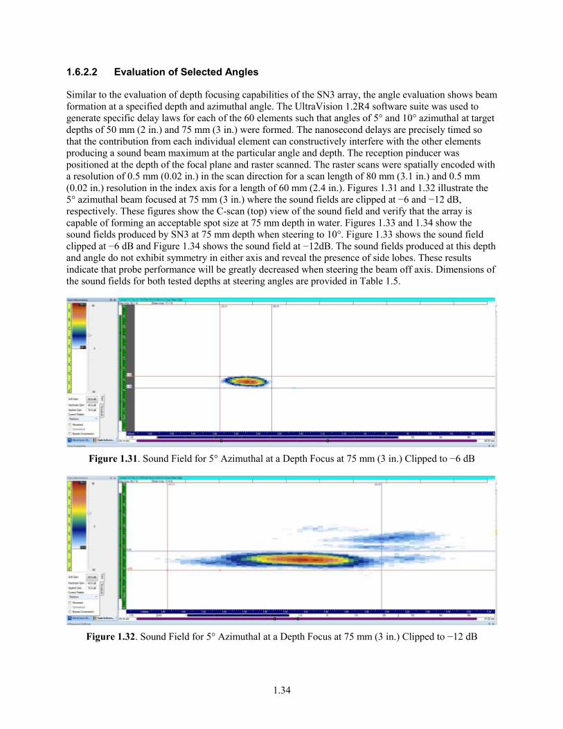
1.34

1.6.2.2 Evaluation of Selected Angles

Similar to the evaluation of depth focusing capabilities of the SN3 array, the angle evaluation shows beam formation at a specified depth and azimuthal angle. The UltraVision 1.2R4 software suite was used to generate specific delay laws for each of the 60 elements such that angles of 5° and 10° azimuthal at target depths of 50 mm (2 in.) and 75 mm (3 in.) were formed. The nanosecond delays are precisely timed so that the contribution from each individual element can constructively interfere with the other elements producing a sound beam maximum at the particular angle and depth. The reception pinducer was positioned at the depth of the focal plane and raster scanned. The raster scans were spatially encoded with a resolution of 0.5 mm (0.02 in.) in the scan direction for a scan length of 80 mm (3.1 in.) and 0.5 mm (0.02 in.) resolution in the index axis for a length of 60 mm (2.4 in.). Figures 1.31 and 1.32 illustrate the 5° azimuthal beam focused at 75 mm (3 in.) where the sound fields are clipped at −6 and −12 dB, respectively. These figures show the C-scan (top) view of the sound field and verify that the array is capable of forming an acceptable spot size at 75 mm depth in water. Figures 1.33 and 1.34 show the sound fields produced by SN3 at 75 mm depth when steering to 10°. Figure 1.33 shows the sound field clipped at −6 dB and Figure 1.34 shows the sound field at −12dB. The sound fields produced at this depth and angle do not exhibit symmetry in either axis and reveal the presence of side lobes. These results indicate that probe performance will be greatly decreased when steering the beam off axis. Dimensions of the sound fields for both tested depths at steering angles are provided in Table 1.5.

Figure 1.31. Sound Field for 5° Azimuthal at a Depth Focus at 75 mm (3 in.) Clipped to −6 dB

Figure 1.32. Sound Field for 5° Azimuthal at a Depth Focus at 75 mm (3 in.) Clipped to −12 dB

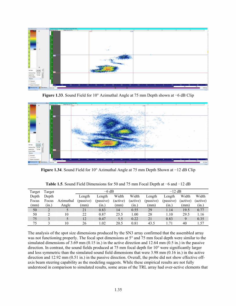
1.35

Figure 1.33. Sound Field for 10° Azimuthal Angle at 75 mm Depth shown at −6 dB Clip

Figure 1.34. Sound Field for 10° Azimuthal Angle at 75 mm Depth Shown at −12 dB Clip

Table 1.5. Sound Field Dimensions for 50 and 75 mm Focal Depth at −6 and −12 dB

Target Depth Focus (mm)

Target Depth Focus (in.)

Azimuthal Angle

−6 dB −12 dB Length

(passive) (mm)

Length (passive)

(in.)

Width (active) (mm)

Width (active)

(in.)

Length (passive)

(mm)

Length (passive)

(in.)

Width (active) (mm)

Width (active)

(in.) 50 2 5 21 0.83 14 0.55 29 1.14 19.5 0.77 50 2 10 22 0.87 25.5 1.00 28 1.10 29.5 1.16 75 3 5 12 0.47 5.5 0.22 21 0.83 9 0.35 75 3 10 26 1.02 20.5 0.81 43.5 1.71 40 1.57

The analysis of the spot size dimensions produced by the SN3 array confirmed that the assembled array was not functioning properly. The focal spot dimensions at 5° and 75 mm focal depth were similar to the simulated dimensions of 3.69 mm (0.15 in.) in the active direction and 12.64 mm (0.5 in.) in the passive direction. In contrast, the sound fields produced at 75 mm focal depth for 10° were significantly larger and less symmetric than the simulated sound field dimensions that were 3.98 mm (0.16 in.) in the active direction and 12.92 mm (0.51 in.) in the passive direction. Overall, the probe did not show effective off-axis beam steering capability as the modeling suggests. While these empirical results are not fully understood in comparison to simulated results, some areas of the TRL array had over-active elements that

1.36

may have contributed to improper phasing of the elements and thereby affected the off-axis beam formation and steering capabilities of the SN3 probe.

1.6.3 Sound Field Dimensional Characterization Analysis for SN3 Prototype Probe

This subsection describes post-fabrication testing and analysis of sound field mapping data obtained in water for the SN3 prototype probe. Sound field dimensions (focal spot size) at −6 dB and −12 dB points at a nominal distance from the face of the probe in water, using a pinducer receiving probe, will be presented, compared, and discussed.

From a review of Subsections 1.6.2.1 and 1.6.2.2, and the data provided in Tables 1.4 and 1.5, it is clear that the sound field dimensions for the focal “spot” size of the prototype array meets acceptance criteria for depth focusing without azimuthal steering. The measured focal spot sizes agree well with the simulated spot sizes presented in Section 1.4. In contrast, the focal spot sizes produced when electronic steering is invoked contradict the predicted spot sizes. These results suggest serious performance degradation when steering the beam off axis.

1.6.4 Spatial Resolution and SNR Analysis for SN3 Prototype Probe

This subsection describes post-fabrication testing of the SN3 prototype probe, focused on the acquisition of ultrasonic data describing the spatial resolution performance for this ETU. Spatial resolution data and testing procedures using raster scanning of the probe and employing flat reflectors with various spacing to evaluate array resolution performance in water are presented. Sound field dimensional analysis is presented and a comparison of the spatial resolution performance of the SN3 probe will be discussed along with results from the FY14 SN2 probe.

A simple resolution target was built from a ¾ in. thick Plexiglas plate. A set of 0.5 in. deep threaded holes were tapped into the plate to allow for the placement of six pairs of 1.5 in. hex socket-head cap screws, placed at different distances from one another. All screws were 28.57 mm (1.125 in.) above the Plexiglas back wall. Each pair of screws was separated 25.4 mm (1.0 in.) apart from the next pair. The pair with the widest center-to-center separation had a distance of 25.4 mm (1.0 in.). The next closest pair was 19.05 mm (0.75 in.), and in descending distance order, subsequent pairs were spaced at 12.7 mm (0.5 in.), 10.16 mm (0.4 in.), 7.62 mm (0.3 in.), and 6.35 mm (0.25 in.), respectively. The screw heads were filled with epoxy and surfaced to provide a flat reflector with a nominal diameter of 5.72 mm (0.225 in.). A digital photograph of the target is provided in Figure 1.35.

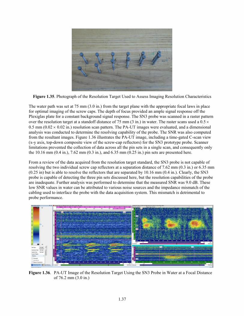
1.37

Figure 1.35. Photograph of the Resolution Target Used to Assess Imaging Resolution Characteristics

The water path was set at 75 mm (3.0 in.) from the target plane with the appropriate focal laws in place for optimal imaging of the screw caps. The depth of focus provided an ample signal response off the Plexiglas plate for a constant background signal response. The SN3 probe was scanned in a raster pattern over the resolution target at a standoff distance of 75 mm (3 in.) in water. The raster scans used a 0.5 × 0.5 mm (0.02 × 0.02 in.) resolution scan pattern. The PA-UT images were evaluated, and a dimensional analysis was conducted to determine the resolving capability of the probe. The SNR was also computed from the resultant images. Figure 1.36 illustrates the PA-UT image, including a time-gated C-scan view (x-y axis, top-down composite view of the screw-cap reflectors) for the SN3 prototype probe. Scanner limitations prevented the collection of data across all the pin sets in a single scan, and consequently only the 10.16 mm (0.4 in.), 7.62 mm (0.3 in.), and 6.35 mm (0.25 in.) pin sets are presented here.

From a review of the data acquired from the resolution target standard, the SN3 probe is not capable of resolving the two individual screw cap reflectors at a separation distance of 7.62 mm (0.3 in.) or 6.35 mm (0.25 in) but is able to resolve the reflectors that are separated by 10.16 mm (0.4 in.). Clearly, the SN3 probe is capable of detecting the three pin sets discussed here, but the resolution capabilities of the probe are inadequate. Further analysis was performed to determine that the measured SNR was 9.0 dB. These low SNR values in water can be attributed to various noise sources and the impedance mismatch of the cabling used to interface the probe with the data acquisition system. This mismatch is detrimental to probe performance.

Figure 1.36. PA-UT Image of the Resolution Target Using the SN3 Probe in Water at a Focal Distance

of 76.2 mm (3.0 in.)

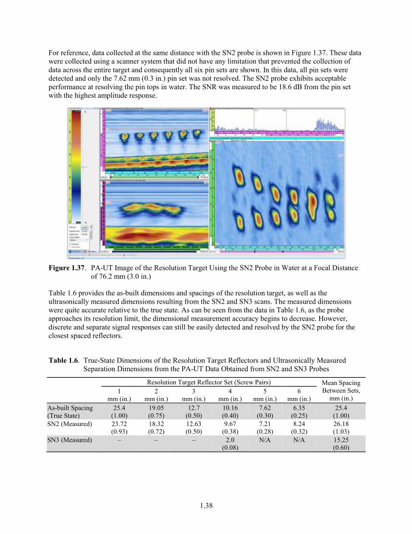
1.38

For reference, data collected at the same distance with the SN2 probe is shown in Figure 1.37. These data were collected using a scanner system that did not have any limitation that prevented the collection of data across the entire target and consequently all six pin sets are shown. In this data, all pin sets were detected and only the 7.62 mm (0.3 in.) pin set was not resolved. The SN2 probe exhibits acceptable performance at resolving the pin tops in water. The SNR was measured to be 18.6 dB from the pin set with the highest amplitude response.

Figure 1.37. PA-UT Image of the Resolution Target Using the SN2 Probe in Water at a Focal Distance

of 76.2 mm (3.0 in.)

Table 1.6 provides the as-built dimensions and spacings of the resolution target, as well as the ultrasonically measured dimensions resulting from the SN2 and SN3 scans. The measured dimensions were quite accurate relative to the true state. As can be seen from the data in Table 1.6, as the probe approaches its resolution limit, the dimensional measurement accuracy begins to decrease. However, discrete and separate signal responses can still be easily detected and resolved by the SN2 probe for the closest spaced reflectors.

Table 1.6. True-State Dimensions of the Resolution Target Reflectors and Ultrasonically Measured Separation Dimensions from the PA-UT Data Obtained from SN2 and SN3 Probes

Resolution Target Reflector Set (Screw Pairs) Mean Spacing Between Sets,

mm (in.) 1

mm (in.) 2

mm (in.) 3

mm (in.) 4

mm (in.) 5

mm (in.) 6

mm (in.) As-built Spacing (True State)

25.4 (1.00)

19.05 (0.75)

12.7 (0.50)

10.16 (0.40)

7.62 (0.30)

6.35 (0.25)

25.4 (1.00)

SN2 (Measured) 23.72 (0.93)

18.32 (0.72)

12.63 (0.50)

9.67 (0.38)

7.21 (0.28)

8.24 (0.32)

26.18 (1.03)

SN3 (Measured) – – – 2.0 (0.08)

N/A N/A 15.25 (0.60)

1.39

1.7 Primary Inspection Parameters for 3D Imaging Assessment

This section of the report defines the primary inspection parameters and critical attributes that provide the criteria for assessing the 3D image performance, functionality, and effectiveness of the SN2 and SN3 PA-UT prototypes. The effort reported here is focused on analyses of data and performance metrics obtained from imaging work conducted with both the SN2 and SN3 prototype ETUs in water and sodium.

In FY15, only the SN2 probe (from FY14) was tested in sodium. The primary inspection parameters and critical attributes for evaluating the 3D image quality of the SN2 probe in sodium included:

1. Inspection time (duration)

2. Number of scanning repetitions

3. Data sampling frequency

4. Sensor-to-target distance

5. Spatial scanning increment size

6. Sodium temperature

7. Wetting of the probe face

8. Thermal cycling

9. Target size and orientation

10. Signal-to-noise ratio

11. Ability to resolve targets in-sodium

With the analyses of data obtained from these performance characterization tests, PNNL was able to quantify key performance parameters that were compared and contrasted between the FY14 tests and the FY15 tests with the SN2 probe for in-sodium tests. Summary highlights of data and imaging results from water and in-sodium tests are provided in Sections 1.8 and 1.9, respectively, and the conclusions obtained from the evaluation of these probes are discussed in Section 1.10.

1.8 Imaging Assessment in Water for SN3 Prototype Probe

This section describes the imaging test and data obtained from the SN3 prototype probe in water (at room temperature) to provide a baseline for determination of whether or not the probe was mature enough to be tested in sodium. The scanning configuration for the water testing, only employed a single resolution target, and has been described previously in Section 1.6.4 and in Braatz et al. (2013). The probe was configured for x-y axes raster scanning in an immersion tank for data acquisition. During scanning, it became apparent that the probe was unable to acquire data with sufficient signal amplitudes to warrant further testing in sodium during FY15. The results provided in Section 1.6.4 show an ultrasonic image resulting from the testing of the SN3 matrix array in water, using the resolution target. It can be seen that the SNR in water is quite low, and noise within the probe coupled with signal losses from cabling and connector matching issues were having a significant impact on the probe’s ability to effectively transmit sufficient energy into the medium. In addition, the low SNR makes it very difficult to detect targets, discriminate relevant signals, and subsequently characterize detected target features.

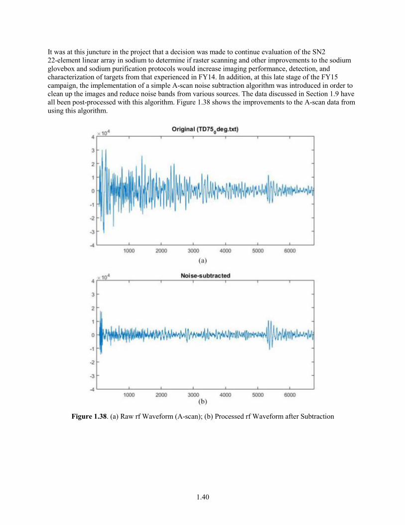
1.40

It was at this juncture in the project that a decision was made to continue evaluation of the SN2 22-element linear array in sodium to determine if raster scanning and other improvements to the sodium glovebox and sodium purification protocols would increase imaging performance, detection, and characterization of targets from that experienced in FY14. In addition, at this late stage of the FY15 campaign, the implementation of a simple A-scan noise subtraction algorithm was introduced in order to clean up the images and reduce noise bands from various sources. The data discussed in Section 1.9 have all been post-processed with this algorithm. Figure 1.38 shows the improvements to the A-scan data from using this algorithm.

Figure 1.38. (a) Raw rf Waveform (A-scan); (b) Processed rf Waveform after Subtraction

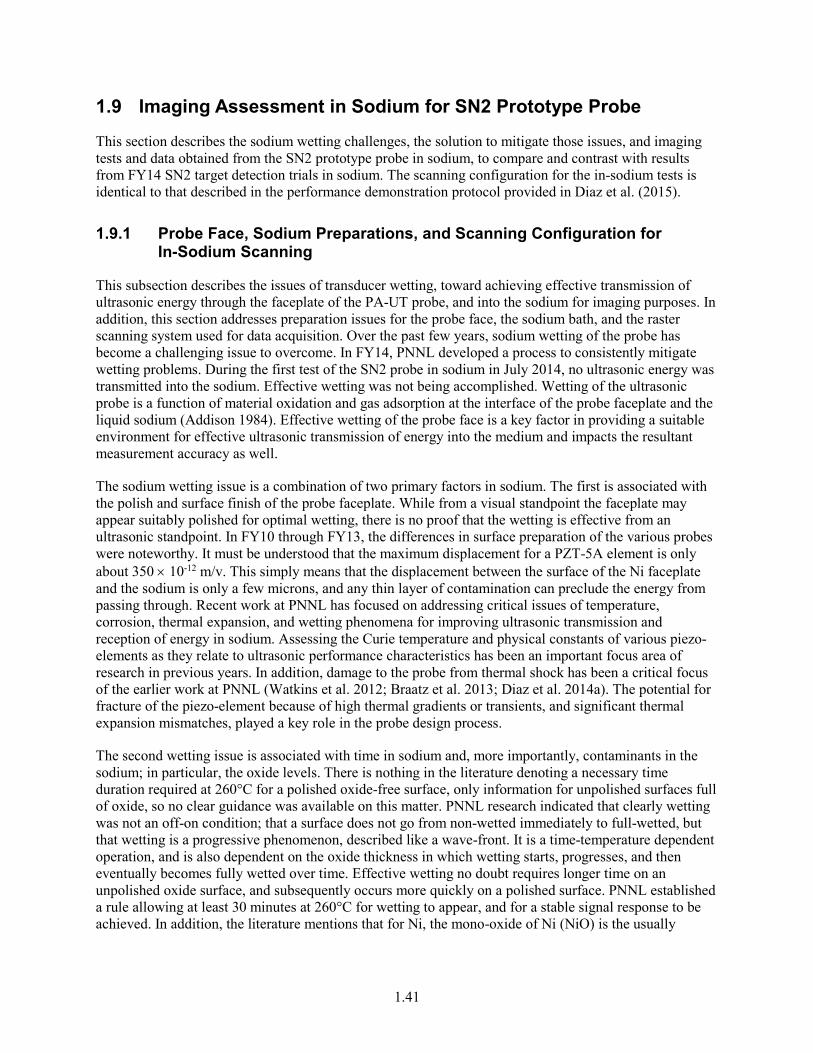
1.41

1.9 Imaging Assessment in Sodium for SN2 Prototype Probe

This section describes the sodium wetting challenges, the solution to mitigate those issues, and imaging tests and data obtained from the SN2 prototype probe in sodium, to compare and contrast with results from FY14 SN2 target detection trials in sodium. The scanning configuration for the in-sodium tests is identical to that described in the performance demonstration protocol provided in Diaz et al. (2015).

1.9.1 Probe Face, Sodium Preparations, and Scanning Configuration for In-Sodium Scanning

This subsection describes the issues of transducer wetting, toward achieving effective transmission of ultrasonic energy through the faceplate of the PA-UT probe, and into the sodium for imaging purposes. In addition, this section addresses preparation issues for the probe face, the sodium bath, and the raster scanning system used for data acquisition. Over the past few years, sodium wetting of the probe has become a challenging issue to overcome. In FY14, PNNL developed a process to consistently mitigate wetting problems. During the first test of the SN2 probe in sodium in July 2014, no ultrasonic energy was transmitted into the sodium. Effective wetting was not being accomplished. Wetting of the ultrasonic probe is a function of material oxidation and gas adsorption at the interface of the probe faceplate and the liquid sodium (Addison 1984). Effective wetting of the probe face is a key factor in providing a suitable environment for effective ultrasonic transmission of energy into the medium and impacts the resultant measurement accuracy as well.

The sodium wetting issue is a combination of two primary factors in sodium. The first is associated with the polish and surface finish of the probe faceplate. While from a visual standpoint the faceplate may appear suitably polished for optimal wetting, there is no proof that the wetting is effective from an ultrasonic standpoint. In FY10 through FY13, the differences in surface preparation of the various probes were noteworthy. It must be understood that the maximum displacement for a PZT-5A element is only about 350 × 10-12 m/v. This simply means that the displacement between the surface of the Ni faceplate and the sodium is only a few microns, and any thin layer of contamination can preclude the energy from passing through. Recent work at PNNL has focused on addressing critical issues of temperature, corrosion, thermal expansion, and wetting phenomena for improving ultrasonic transmission and reception of energy in sodium. Assessing the Curie temperature and physical constants of various piezo-elements as they relate to ultrasonic performance characteristics has been an important focus area of research in previous years. In addition, damage to the probe from thermal shock has been a critical focus of the earlier work at PNNL (Watkins et al. 2012; Braatz et al. 2013; Diaz et al. 2014a). The potential for fracture of the piezo-element because of high thermal gradients or transients, and significant thermal expansion mismatches, played a key role in the probe design process.

The second wetting issue is associated with time in sodium and, more importantly, contaminants in the sodium; in particular, the oxide levels. There is nothing in the literature denoting a necessary time duration required at 260°C for a polished oxide-free surface, only information for unpolished surfaces full of oxide, so no clear guidance was available on this matter. PNNL research indicated that clearly wetting was not an off-on condition; that a surface does not go from non-wetted immediately to full-wetted, but that wetting is a progressive phenomenon, described like a wave-front. It is a time-temperature dependent operation, and is also dependent on the oxide thickness in which wetting starts, progresses, and then eventually becomes fully wetted over time. Effective wetting no doubt requires longer time on an unpolished oxide surface, and subsequently occurs more quickly on a polished surface. PNNL established a rule allowing at least 30 minutes at 260°C for wetting to appear, and for a stable signal response to be achieved. In addition, the literature mentions that for Ni, the mono-oxide of Ni (NiO) is the usually

1.42

expected species and is expected to dissolve, but that at high solubility levels of O2 in sodium, the ternary oxides of Ni have been seen, NaNiO2 and Na2NiO2. It says some ternary oxides can be more stable, and particularly more stable when high O2 levels are present. It does say that the Ni ternary oxides are expected to dissolve, but this still may be O2-level-dependent (Addison 1984). From trials performed at PNNL in FY13 and FY14, it has been shown that excessive levels of O2 (>3 ppm) are sufficient to preclude effective wetting on the PA-UT probe faces. In order to address these issues, PNNL developed a process for effective surface preparation and polishing of the Ni faceplate of the probe prior to in-sodium testing. This process has been well documented in Diaz et al. (2014b) and Diaz et al. (2015).

Modifications to the sodium containment were made early in FY15. Heating of the sodium bath has been modified to incorporate a custom heater block and temperature controller. In addition, two custom-made sodium test vessels were fabricated. The entire system (heater block, temperature controller, and reaction test vessel) were evaluated and made fully operational in the spring of FY15. In FY14 the cabling for the ultrasonic probe and the scanner platform were inserted into the glovebox through a very small pass-through port. This port was modified to allow for a larger volume of cables as required by the FY15 data acquisition system and probe configuration. Also, large quantities of fresh sodium were procured for FY15 testing and all sodium went through a filtration process prior to use in tests.

Finally, in FY15, PNNL completed the design, fabrication, and testing of an upgraded USV scanner and controller platform for in-sodium tests. This platform was designed to provide an x-y axes raster scanning capability for PA-UT probes in sodium. In large part, it was determined in FY14 that polar (rotational) scanning of a PA-UT probe from a fixed point was insufficient for obtaining suitable amounts of specular energy and the required level of redundancy from targets immersed in sodium. In FY15, PNNL decided to invoke a raster scanning capability to translate the PA-UT probe directly over the target region of interest, and simultaneously examine the target over a range of inspection angles. Not only does this configuration provide richer ultrasonic data because of multiple points of insonification over the area of interest, but the data are visualized and presented in a much improved image that is easier to interpret. The photographs provided in Figure 1.39 show the portable, rack-mounted scanning controller and 3-axis (x-, y- and z-axes) scanner platform for use in both laboratory and sodium glovebox applications. This scanning platform provides mechanical scanning accuracy in the x- and y-axes of 0.025 mm.

This scanning platform was transported to the laboratory facility where the sodium glovebox resides, and was configured for operation just outside the glovebox. Cabling from the instrument control rack was tethered through the port, and connected to the scanner platform that was already positioned inside the glovebox over the sodium containment vessel. The vessel is pre-configured with the target placed at the bottom, and centered in the containment vessel. After pre-polishing of the probe face, the probe was covered and sealed, and then inserted through the port. These distances require long cable lengths that do affect signal amplitude because of attenuation. Once the probe and cables are routed inside the glovebox, the port is sealed and the argon atmosphere is re-established. A final polishing is conducted on the probe face as per the protocol defined in Diaz et al. (2015). Photographs of these steps are provided in Figures 1.40 through 1.43. Because these photographs are taken through a thick Plexiglas window, the clarity of these images is non-optimal.

1.43

Figure 1.39. Left: Rack Mounted Scan Controller Instrumentation and Motor Drivers. Middle: Top

View of 3-Axis Raster Scan Platform. Right: Side View of 3-Axis Raster Scan Platform.

Figure 1.40. Images of Wrapped and Sealed SN2 Probe after Pre-polishing, Prior to Insertion into the

Sodium Glovebox

1.44

Figure 1.41. Rack-Mounted Scanning Controller System, Configured for Use Near the Sodium

Glovebox

1.45

Figure 1.42. Scanning Platform, Configured over the Sodium Containment Vessel within the Sodium

Glovebox

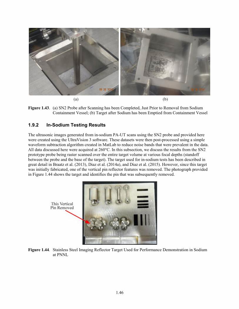
1.46

Figure 1.43. (a) SN2 Probe after Scanning has been Completed, Just Prior to Removal from Sodium

Containment Vessel; (b) Target after Sodium has been Emptied from Containment Vessel

1.9.2 In-Sodium Testing Results

The ultrasonic images generated from in-sodium PA-UT scans using the SN2 probe and provided here were created using the UltraVision 3 software. These datasets were then post-processed using a simple waveform subtraction algorithm created in MatLab to reduce noise bands that were prevalent in the data. All data discussed here were acquired at 260°C. In this subsection, we discuss the results from the SN2 prototype probe being raster scanned over the entire target volume at various focal depths (standoff between the probe and the base of the target). The target used for in-sodium tests has been described in great detail in Braatz et al. (2013), Diaz et al. (2014a), and Diaz et al. (2015). However, since this target was initially fabricated, one of the vertical pin reflector features was removed. The photograph provided in Figure 1.44 shows the target and identifies the pin that was subsequently removed.

Figure 1.44. Stainless Steel Imaging Reflector Target Used for Performance Demonstration in Sodium

at PNNL

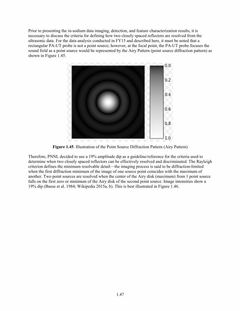
1.47

Prior to presenting the in-sodium data imaging, detection, and feature characterization results, it is necessary to discuss the criteria for defining how two closely spaced reflectors are resolved from the ultrasonic data. For the data analysis conducted in FY15 and described here, it must be noted that a rectangular PA-UT probe is not a point source; however, at the focal point, the PA-UT probe focuses the sound field as a point source would be represented by the Airy Pattern (point source diffraction pattern) as shown in Figure 1.45.

Figure 1.45. Illustration of the Point Source Diffraction Pattern (Airy Pattern)

Therefore, PNNL decided to use a 19% amplitude dip as a guideline/reference for the criteria used to determine when two closely spaced reflectors can be effectively resolved and discriminated. The Rayleigh criterion defines the minimum resolvable detail—the imaging process is said to be diffraction-limited when the first diffraction minimum of the image of one source point coincides with the maximum of another. Two point sources are resolved when the center of the Airy disk (maximum) from 1 point source falls on the first zero or minimum of the Airy disk of the second point source. Image intensities show a 19% dip (Busse et al. 1984; Wikipedia 2015a, b). This is best illustrated in Figure 1.46.

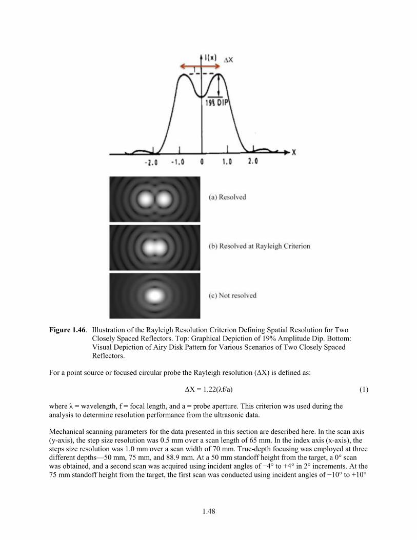
1.48

Figure 1.46. Illustration of the Rayleigh Resolution Criterion Defining Spatial Resolution for Two

Closely Spaced Reflectors. Top: Graphical Depiction of 19% Amplitude Dip. Bottom: Visual Depiction of Airy Disk Pattern for Various Scenarios of Two Closely Spaced Reflectors.

For a point source or focused circular probe the Rayleigh resolution (∆X) is defined as:

∆X = 1.22(λf/a) (1)

where λ = wavelength, f = focal length, and a = probe aperture. This criterion was used during the analysis to determine resolution performance from the ultrasonic data.

Mechanical scanning parameters for the data presented in this section are described here. In the scan axis (y-axis), the step size resolution was 0.5 mm over a scan length of 65 mm. In the index axis (x-axis), the steps size resolution was 1.0 mm over a scan width of 70 mm. True-depth focusing was employed at three different depths—50 mm, 75 mm, and 88.9 mm. At a 50 mm standoff height from the target, a 0° scan was obtained, and a second scan was acquired using incident angles of −4° to +4° in 2° increments. At the 75 mm standoff height from the target, the first scan was conducted using incident angles of −10° to +10°

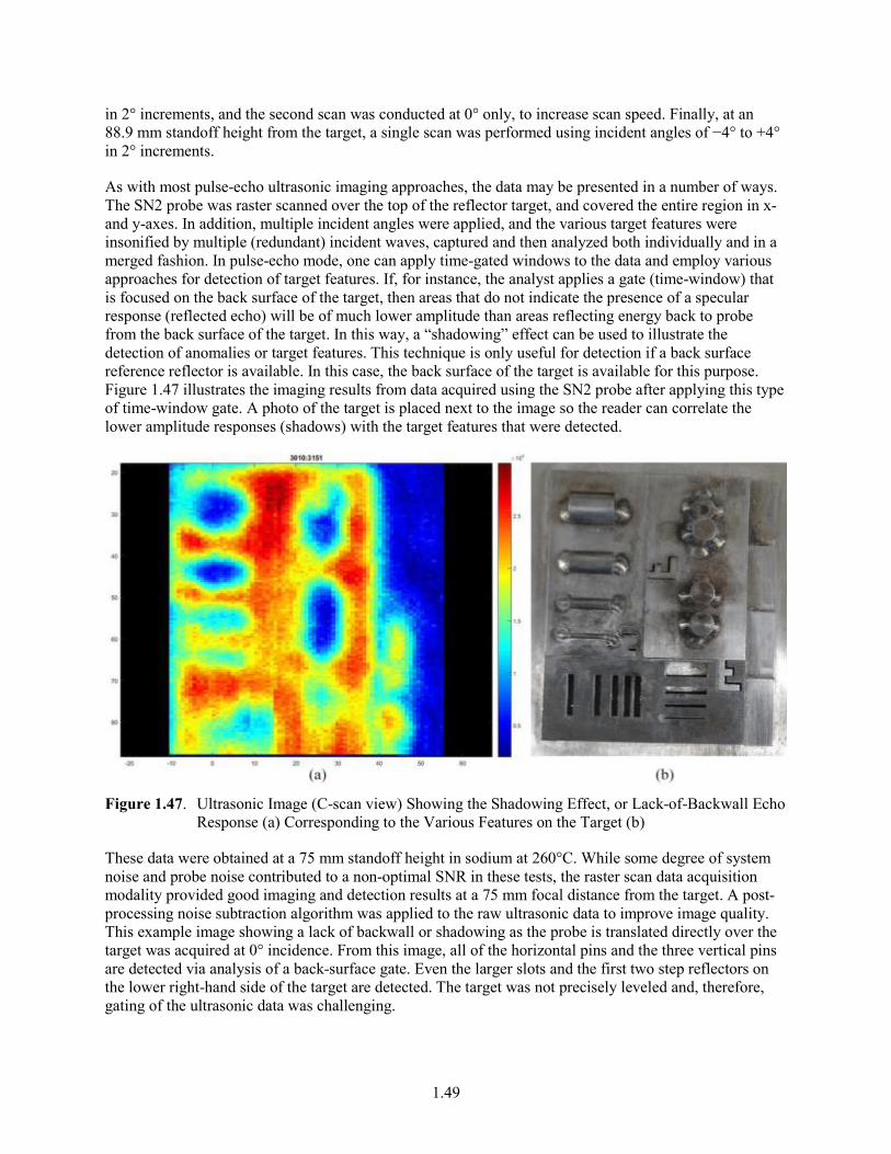
1.49

in 2° increments, and the second scan was conducted at 0° only, to increase scan speed. Finally, at an 88.9 mm standoff height from the target, a single scan was performed using incident angles of −4° to +4° in 2° increments.

As with most pulse-echo ultrasonic imaging approaches, the data may be presented in a number of ways. The SN2 probe was raster scanned over the top of the reflector target, and covered the entire region in x- and y-axes. In addition, multiple incident angles were applied, and the various target features were insonified by multiple (redundant) incident waves, captured and then analyzed both individually and in a merged fashion. In pulse-echo mode, one can apply time-gated windows to the data and employ various approaches for detection of target features. If, for instance, the analyst applies a gate (time-window) that is focused on the back surface of the target, then areas that do not indicate the presence of a specular response (reflected echo) will be of much lower amplitude than areas reflecting energy back to probe from the back surface of the target. In this way, a “shadowing” effect can be used to illustrate the detection of anomalies or target features. This technique is only useful for detection if a back surface reference reflector is available. In this case, the back surface of the target is available for this purpose. Figure 1.47 illustrates the imaging results from data acquired using the SN2 probe after applying this type of time-window gate. A photo of the target is placed next to the image so the reader can correlate the lower amplitude responses (shadows) with the target features that were detected.

Figure 1.47. Ultrasonic Image (C-scan view) Showing the Shadowing Effect, or Lack-of-Backwall Echo

Response (a) Corresponding to the Various Features on the Target (b)

These data were obtained at a 75 mm standoff height in sodium at 260°C. While some degree of system noise and probe noise contributed to a non-optimal SNR in these tests, the raster scan data acquisition modality provided good imaging and detection results at a 75 mm focal distance from the target. A post-processing noise subtraction algorithm was applied to the raw ultrasonic data to improve image quality. This example image showing a lack of backwall or shadowing as the probe is translated directly over the target was acquired at 0° incidence. From this image, all of the horizontal pins and the three vertical pins are detected via analysis of a back-surface gate. Even the larger slots and the first two step reflectors on the lower right-hand side of the target are detected. The target was not precisely leveled and, therefore, gating of the ultrasonic data was challenging.

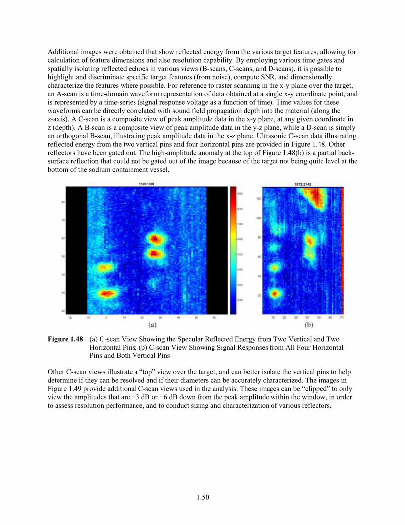
1.50

Additional images were obtained that show reflected energy from the various target features, allowing for calculation of feature dimensions and also resolution capability. By employing various time gates and spatially isolating reflected echoes in various views (B-scans, C-scans, and D-scans), it is possible to highlight and discriminate specific target features (from noise), compute SNR, and dimensionally characterize the features where possible. For reference to raster scanning in the x-y plane over the target, an A-scan is a time-domain waveform representation of data obtained at a single x-y coordinate point, and is represented by a time-series (signal response voltage as a function of time). Time values for these waveforms can be directly correlated with sound field propagation depth into the material (along the z-axis). A C-scan is a composite view of peak amplitude data in the x-y plane, at any given coordinate in z (depth). A B-scan is a composite view of peak amplitude data in the y-z plane, while a D-scan is simply an orthogonal B-scan, illustrating peak amplitude data in the x-z plane. Ultrasonic C-scan data illustrating reflected energy from the two vertical pins and four horizontal pins are provided in Figure 1.48. Other reflectors have been gated out. The high-amplitude anomaly at the top of Figure 1.48(b) is a partial back-surface reflection that could not be gated out of the image because of the target not being quite level at the bottom of the sodium containment vessel.

Figure 1.48. (a) C-scan View Showing the Specular Reflected Energy from Two Vertical and Two

Horizontal Pins; (b) C-scan View Showing Signal Responses from All Four Horizontal Pins and Both Vertical Pins

Other C-scan views illustrate a “top” view over the target, and can better isolate the vertical pins to help determine if they can be resolved and if their diameters can be accurately characterized. The images in Figure 1.49 provide additional C-scan views used in the analysis. These images can be “clipped” to only view the amplitudes that are −3 dB or −6 dB down from the peak amplitude within the window, in order to assess resolution performance, and to conduct sizing and characterization of various reflectors.

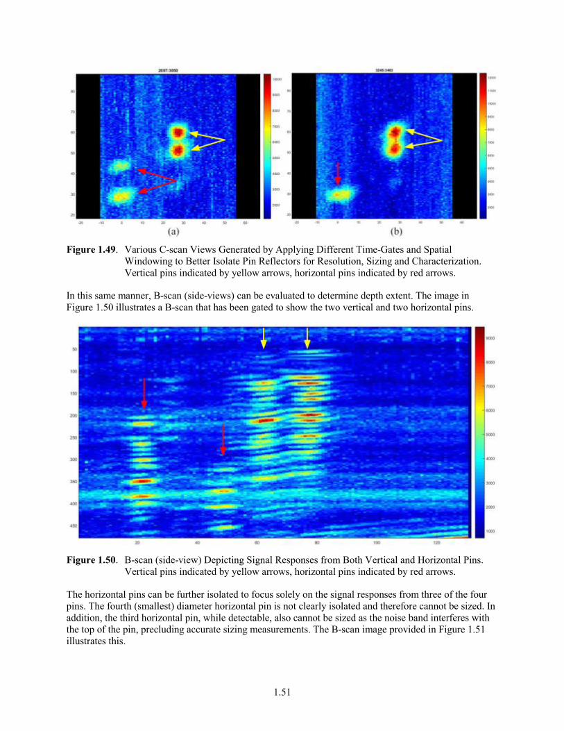
1.51

Figure 1.49. Various C-scan Views Generated by Applying Different Time-Gates and Spatial

Windowing to Better Isolate Pin Reflectors for Resolution, Sizing and Characterization. Vertical pins indicated by yellow arrows, horizontal pins indicated by red arrows.

In this same manner, B-scan (side-views) can be evaluated to determine depth extent. The image in Figure 1.50 illustrates a B-scan that has been gated to show the two vertical and two horizontal pins.

Figure 1.50. B-scan (side-view) Depicting Signal Responses from Both Vertical and Horizontal Pins.

Vertical pins indicated by yellow arrows, horizontal pins indicated by red arrows.

The horizontal pins can be further isolated to focus solely on the signal responses from three of the four pins. The fourth (smallest) diameter horizontal pin is not clearly isolated and therefore cannot be sized. In addition, the third horizontal pin, while detectable, also cannot be sized as the noise band interferes with the top of the pin, precluding accurate sizing measurements. The B-scan image provided in Figure 1.51 illustrates this.

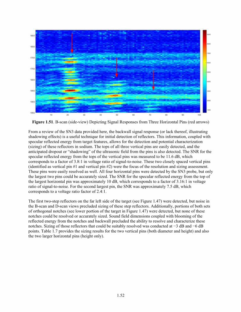
1.52

Figure 1.51. B-scan (side-view) Depicting Signal Responses from Three Horizontal Pins (red arrows)

From a review of the SN3 data provided here, the backwall signal response (or lack thereof, illustrating shadowing effects) is a useful technique for initial detection of reflectors. This information, coupled with specular reflected energy from target features, allows for the detection and potential characterization (sizing) of these reflectors in sodium. The tops of all three vertical pins are easily detected, and the anticipated dropout or “shadowing” of the ultrasonic field from the pins is also detected. The SNR for the specular reflected energy from the tops of the vertical pins was measured to be 11.6 dB, which corresponds to a factor of 3.8:1 in voltage ratio of signal-to-noise. These two closely spaced vertical pins (identified as vertical pin #1 and vertical pin #2) were the focus of the resolution and sizing assessment. These pins were easily resolved as well. All four horizontal pins were detected by the SN3 probe, but only the largest two pins could be accurately sized. The SNR for the specular reflected energy from the top of the largest horizontal pin was approximately 10 dB, which corresponds to a factor of 3.16:1 in voltage ratio of signal-to-noise. For the second largest pin, the SNR was approximately 7.5 dB, which corresponds to a voltage ratio factor of 2.4:1.

The first two-step reflectors on the far left side of the target (see Figure 1.47) were detected, but noise in the B-scan and D-scan views precluded sizing of these step reflectors. Additionally, portions of both sets of orthogonal notches (see lower portion of the target in Figure 1.47) were detected, but none of these notches could be resolved or accurately sized. Sound field dimensions coupled with blooming of the reflected energy from the notches and backwall precluded the ability to resolve and characterize these notches. Sizing of those reflectors that could be suitably resolved was conducted at −3 dB and −6 dB points. Table 1.7 provides the sizing results for the two vertical pins (both diameter and height) and also the two larger horizontal pins (height only).

1.53

Table 1.7. Vertical and Horizontal Pin Sizing Results

Pin Description Pin

Orientation True-State Dimension

(mm)

−3 dB Measured Diameter

(mm)

−6 dB Measured Diameter

(mm)

−6 dB Measured

Height (mm)

Pin #1 Vertical 6 diameter; 11 height 4.75 8.25 9.9 Pin #2 Vertical 6 diameter; 11 height 4.5 7.75 9.9 Largest Horizontal 9 height/diameter -- -- 8.7 Second Largest Horizontal 6 height/diameter -- -- 5.6

1.10 Discussion and Conclusions

This TLR provides a summary of the work conducted at PNNL in FY15 on the under-sodium viewing project, including a performance evaluation of the SN3 matrix-array PA-UT ETU probe. This evaluation established the foundation for determining the viability of conducting in-sodium tests with the SN3 probe in FY15. In addition, this TLR provides the results from a performance demonstration test using the SN2 ETU probe for target detection trials in sodium at 260°C. The activities conducted during this assessment focused on evaluating the performance characteristics and employing the primary inspection parameters described in Sections 1.3, 1.5 and 1.7 for in-sodium target detection trials.

During the first part of FY15, the PNNL designed, fabricated, and tested a 60-element TRL, matrix array, PA-UT probe and completed a set of performance evaluation tests to quantify the probe’s capabilities for target detection and characterization. A set of pre-fabrication pulse-echo tests on individual array elements (in water) were conducted, followed by a set of post-fabrication pulse-echo testing on individual array elements, also in water. This included measurements to validate the array pin connections, the transmit uniformity for each element, the cross talk (to assess inter-element coupling between neighboring elements), and an evaluation of selected depth focus points and angles (to assess how effectively the probe can skew the sound field off its 0° primary axis). Traditionally, PNNL at this stage of the evaluation would have conducted an assessment of temperature resistance and thermal cycling effects (in hot oil); however, it was determined that the probe was not mature enough to warrant high-temperature tests. A number of laboratory measurements and performance characterization scans were, however, conducted to quantify a set of critical attributes used as metrics for assessing and comparing probe performance and capabilities to the SN2 probe developed and tested in FY14. Key efforts included the acquisition of:

1. Individual voltage responses from each element after employing a standard excitation pulse, and received with a broadband pinducer for receiving signal responses.

2. Center and peak frequency responses from the FFTs of individual elements

3. −6 dB BWs of each element

4. Sound field dimensions (focal spot size) at −6 dB and −12 dB points at a nominal distance from the face of the probe in water using a pinducer receiving probe

5. Spatial resolution testing using raster scanning of the probe and employing flat reflectors with various spacings to evaluate array resolution performance in water

1.54

6. Evaluation of signal-to-noise ratio from both pre-fabrication testing of the individual elements and post-fabrication tests.

With the analyses of data obtained from these performance characterization tests, PNNL was able to quantify key performance parameters that were compared and contrasted between the two ETU probes, SN2 and SN3. In particular, sound field dimensions (spot size), resolution capabilities, SNR, frequency response, and BW characteristics constitute the suite of critical attributes used to evaluate these probes. In this discussion, the reader is referred to Diaz et al. (2014b) for pertinent characterization information associated with the SN2 probe.

From a review of the data provided in Sections 1.5 and 1.6, coupled with the results of Diaz et al. (2014b), it is clear that the various stages of fabrication and the materials and quality of the processes employed for construction of the elements, backing, soldering, and bonding, can all have critical impact on probe performance. Prior to fabrication of the housed SN3 probe array, it was shown that the SN3 probe had inherently lower noise levels and an improved SNR for the individual elements over that of the SN2 probe; on the order of 4–6 dB. In addition, all 60 elements were functional and operating properly. After fabrication and housing, as each element was being validated for connectivity, it was found that 59 of 60 elements were confirmed to be operational for the SN3 probe at the time these data were taken; however, some elements had a reduced level of efficient performance from an energy transmission perspective, and a significant amount of noise had been introduced from various sources. These sources are not yet well understood, but likely include grounding issues, electrical impedance matching issues with wires, connectors and cables, probe noise and motor/system noise. These noise sources, when combined, have a significant effect on the overall signal amplitudes of the post-fabricated SN3 probe. In addition, element #18 was found to be non-operational for the SN3 probe during the late FY15 portion of the performance characterization tests. One element out of 60 was determined to be inconsequential to the overall performance of the probe.

An assessment of the transmit uniformity on an element-by-element basis was conducted, and these measurements established a foundation for assessing areas of the arrays that were not emitting energy in an efficient manner, or where areas were dis-bonded. The SN2 array clearly illustrated some areas of complete dis-bonding where no ultrasonic energy was being emitted, but this did not have a significant effect on the overall performance of the probe, in comparison to the SN3 probe. While the overall activity of all elements (59 of 60) of the SN3 probe were demonstrated, and there was no evidence of dis-bonding over the aperture of the SN3 array, it was noted that there were elements that emitted significantly more acoustic energy than others across the 60 elements of the SN3 array. Laboratory measurements provided valuable dimensional data associated with the sound fields, and an assessment of the element-to-element cross talk showed that inter-element ultrasonic leakage was more effectively isolated for the SN3 probe over that of the SN2 probe (−26 dB as opposed to −13 dB). The SN3 probe exhibited much improved element-to-element isolation, and from a measurement perspective, the cross talk between individual elements in the 60-element SN3 probe was barely detectable. This means that the elements were truly isolated more effectively than in the SN2 probe. While both probes showed suitable capabilities for demonstrating effectiveness at generating sound fields with the appropriate focal depths and dimensions, the SN2 probe illustrated the capability to skew its primary sound field lobe over the designed range of angles (−15° to +15°) more effectively than the SN3 probe. This ability to effectively control off-axis beam steering is critical for a PA-UT probe. Phasing issues associated with individual elements having too much variability in sensitivity to the voltage excitation played a role in the reduced sound field coherence at off-angles with the SN3 probe.

Between FY14 and FY15, data were acquired to conduct an assessment of the amplitude and frequency response, BW, SNR, and element sensitivity for both probes. Individual voltage responses from each

1.55

element after employing a standard excitation pulse were captured with a pinducer for later analysis. The most obvious difference of significance between the two probes was in the signal amplitudes and general SNRs. While the operational frequencies were generally identical, the SN2 prototype array generated significantly higher sonic intensities (signal amplitudes) than the SN3 probe. The source of this difference is not fully understood, but in theory, larger piezo-elements will generate higher amplitude signal voltages over smaller piezo-elements. The 22-element linear SN2 array was comprised of individual elements with an area of 15 mm2. The individual element size of the 60 element matrix SN3 array was only 3.24 mm2. Because the SN2 array operated in pulse-echo mode, the entire aperture of the probe is employed for generating the sound field at any given focal distance, and is used to compute the effective piezo-element area responsible for transmission of ultrasonic energy. In the case of the SN3 TRL array, only half of the total probe aperture is employed for transmission of ultrasonic energy, so this translates to an effective total piezo-element area of 97.2 mm2. This is compared to an effective total piezo-element area for the SN2 probe of 330 mm2. The SN2 probe has a factor of 3.4 times the active piezo-element energy transmission area of the SN3 probe for actively generating ultrasonic energy. Coupled with the noise factors mentioned earlier, it was determined that the SN3 probe needed more work to be ready for performance demonstration in sodium in FY15.

From an analysis of the sound fields of both probes, it is clear that the sound field dimensions for the focal “spot” size of the two probes are slightly different, as was anticipated, based upon simulation and modeling results described earlier. The data showed that the SN3 probe has a sound field that is slightly improved (smaller, tighter sound field) over that of the SN2 probe in both passive and active element dimensions (length and width, respectively). With regard to resolution performance, the SN3 probe should (in theory) be capable of resolving all of the reflectors provided by the resolution target described in Section 1.6.4. However, the data show that the SN3 probe is not capable of resolving the reflectors that are separated by a distance of 7.62 mm (0.3 in.), or the reflectors that are separated by a distance of 6.35 mm (0.25 in.). The SN3 probe was able to resolve the reflectors separated by 10.16 mm (0.4 in.). The SN2 probe is capable of resolving the closest set of reflectors that are separated by 6.35 mm (0.25 in.). Only the SN2 probe demonstrated suitable detection and characterization (sizing) capability, based on the original design specifications, and it is shown that the SN2 probe has an improved resolution capability over that of the SN3 prototype probe. In large part, this is likely because of the high noise issues and low signal amplitudes generated by the SN3 probe. Throughout testing, much effort was put forth to try to reduce noise by systematically isolating and measuring various points in the system to identify areas that were contributing to the noise in the signals. In addition, bandpass filtering was applied throughout the data acquisition effort. A low-pass filter of 5 MHz and a high-pass filter of 500 kHz were applied to condition the signals in an effort to reduce noise and improve SNR. Finally, in evaluating the SNR from the water data obtained in this study, the SNR for the SN3 probe was measured to be 9 dB and the SNR for the SN2 probe was measured to be 18.6 dB. This corresponds to a difference of 9.6 dB, which corresponds to a voltage ratio difference of 3.02-to-1. The SN2 probe demonstrated a superior post-fabrication SNR level, over that of the SN3 probe, even with some areas of the SN2 probe operating at non-optimal levels (Diaz et al. 2014b).

The effects of temperature and thermal cycling on the SN3 probe were not assessed. The maturity and technical readiness of the SN3 probe was deemed too low to test any further. Therefore, at this point in the project (early August 2015) plans to conduct performance demonstration tests with the SN3 probe were scrapped. Instead, the SN2 probe was readied for additional PD tests in sodium.

While many key performance parameters and critical attributes exist to quantify the performance of a PA-UT probe, the primary characteristics are those that best describe the capability of a probe to effectively detect, resolve, and characterize the reflectors or anomalies required for identification during an examination. In light of the results in FY15 with the SN3 probe, PNNL continued efforts in late FY15

1.56

to pursue in-sodium testing of the SN2 probe to demonstrate that the next critical challenge is to overcome the wetting issue of the probe in sodium. It is believed that this issue, coupled with an inability to raster scan the probe over the target area, was the primary sources of the poor SNR and poor imaging performance of the SN2 probe in FY14. The best data obtained in FY15 performance demonstration tests came from 0° incident sound fields and shallow angled data between −4° and +4°.

During the latter portion of FY15, PNNL assessed the SN2 probe in sodium. With regard to inspection time (duration), sodium temperature, and thermal cycling, this probe provided the required level of robustness to withstand any negative effects that could potentially impact probe performance. In FY14 the SN2 probe was tested in water after the in-sodium target detection trials were completed, and this probe demonstrated normal functionality and operability, verifying that no damage was incurred during in-sodium testing from temperature, thermal cycling, or the duration of testing in the glovebox in FY14. In FY15, the SN2 probe spent an additional 5+ hours of time in sodium at 260°C. This probe now has 12+ hours of performance, immersed in sodium at 260°C, with no measurable decline in functionality or performance. This is a key positive result of USV developments at PNNL. In addition, and for the first time, the SN2 probe was provided the opportunity to function at its designed focal distance and operate in a raster scan modality, increasing the effectiveness of insonification through direct translation of the probe over the entire target area. The imaging, detection, resolution, and characterization results from the target were drastically improved over what was previously achieved in any earlier year.

In FY15 wetting of the sodium became much less of a factor because of lessons learned and enhanced processes and protocols for maintaining effective wetting of the Ni faceplate in sodium. From a review of the data obtained in sodium, it is clear that the SN2 probe showed an improved ability to detect all of the vertical and horizontal pins. Additionally, the probe showed the capability to resolve and accurately characterize the two vertical pins (pin #1 and pin #2) of the target, and also the two largest horizontal pins. Sizing of the pin spacing was more accurate and the SNR was greatly improved. In FY14, this very same probe was not capable of detecting the pin tops because no specular reflected energy was received from the top of the pins. In FY15, the SNR from direct reflected energy off the pin tops was nearly 12 dB. This corresponds to an increase of nearly 4 times the signal sensitivity over the performance from last year. The metrics of SNR and signal dropout (shadowing) indicate an improved ability of the probe to detect the zones where the pins reside, and to capture a backwall signal with higher amplitude signal responses. The two closely spaced vertical pins are separated by a distance of 1.23 mm (edge-to-edge). The longitudinal wave mode speed of sound in liquid sodium at 260°C is 2460 m/s. Using the average center frequency of the SN2 probe (1.61 MHz), the wavelength in sodium for the SN2 probe is given by the equation:

λ = c / f (2)

where λ = wavelength, c = speed of sound, and f = frequency.

Thus, the wavelength in sodium for the SN2 probe is computed as 1.53 mm. Therefore, the edge-to-edge spacing between vertical pin #1 and pin #2 is less than a wavelength. From a review of the sodium data, the measured pin separation from ultrasonic images captured at 260°C was 1.5 mm at the −6 dB point. So, the SN2 probe was capable of measuring the edge-to-edge distance between the two vertical pins to within 0.22 mm of the true-state separation. The fact that the SN2 probe was capable of resolving two reflectors spaced less than 1λ apart is an outstanding result. In addition, the data show that the probe was capable of measuring the heights of the pins (the vertical pins and the two larger horizontal pins) to within 10% or less of their true state. Sizing of the vertical pin diameters was slightly less accurate, but this was expected because of the physical size of the sound fields in the passive axis relative to the vertical pin dimensions.

1.57

PNNL assessed both probes using identical data acquisition and operational parameters. With the analyses of data obtained from these target-detection tests, PNNL was able to identify specific performance improvements between the two ETU probes, and also identify areas where more work needs to be done, if the SN3 design is deemed worthy of future evolution. In particular, major improvements in detection capability, resolution capability, SNR, and environmental robustness were identified with the SN2 probe in FY15. Now, PNNL has concluded that the primary drivers inhibiting the achievement of suitable detection and resolution capabilities in sodium are:

• Achieving a suitable array design that optimizes the balance between element size, number of elements, and matrix specifications for generating a higher energy sound field that is more symmetric and tighter in both passive and active axes

• Control of noise sources, including grounding noise, internal probe noise, cable/connector noise, and system/motor noise

• A capability to steer and control this well-focused beam within reasonable limits

• The ability to raster scan the probe over the entire target area to increase reflected energy redundancy and enhance imaging reconstruction and interpretation.

The last bullet (limitation) was addressed by PNNL in FY15, and the remaining three bullets will be the focus of work in FY16. In FY16, the primary challenge is to increase sound field propagation and image resolution in sodium by designing an array that provides a tighter, more symmetric and more focused sound field (spot size and depth of field). The decision to invoke separate transmit and receive arrays with the TRL SN3 probe design did not result in enough isolation to reduce noise sources. The pulse-echo design may likely be the most advantageous design for this application. A more symmetric 2D pulse-echo matrix array design will improve resolution and sensitivity, while increasing signal strength due to larger element sizes. In addition, this will provide a suitable ability to control/steer the sound field, focus more energy with essentially the same aperture of the 1D linear array design, and improve sound field focal dimensions. The FY16 effort will also focus on reduction of noise sources and custom designed cables from international phased array experts in France. This design will allow for an electronic scanning capability as well.

2.1

2.0 References

Addison CC. 1984. The Chemistry of the Liquid Alkali Metals. John Wiley & Sons Ltd, New York.

ASTM E1065/E1065M-14. 2014. "Standard Practice for Evaluating Characteristics of Ultrasonic Search Units." ASTM International, West Conshohocken, Pennsylvania. DOI 10.1520/E1065-08. www.astm.org.

ASTM E2491-13. 2013. "Standard Guide for Evaluating Performance Characteristics of Phased-Array Ultrasonic Testing Instruments and Systems." ASTM International, West Conshohocken, Pennsylvania. www.astm.org.

Braatz BG, CL Aardahl, DL Baldwin, AD Cinson, JL Fernandes, AM Jones, PE Keller, MR Larche, R Mathews, CA Mullen, AF Pardini, GJ Posakony, ML Watkins, HT Chien, WP Lawrence, DM Engel and SH Sheen. 2013. FY2013 Joint Technical Report on Progress in Development of Ultrasonic Under-Sodium Viewing Technology to Enable Inspection Systems for In-Service Inspection and Repair of Liquid Metal Fast Reactors. PNNL-22872, Pacific Northwest National Laboratory, Richland, Washington.

Busse LJ, HD Collins and SR Doctor. 1984. Review and Discussion of the Development of Synthetic Aperture Focusing Technique for Ultrasonic Testing, SAFT UT. NUREG/CR-3625, PNL-4957, U.S. Nuclear Regulatory Commission, Washington, D.C.

Diaz AA, DL Baldwin, CE Chamberlin, AD Cinson, MK Edwards, TS Hartman, AM Jones, MR Larche, R Mathews, CA Mullen, AF Pardini, GJ Posakony, MS Prowant, HT Chien, DM Engel, WP Lawrence and SH Sheen. 2014a. FY 2014 Joint Technical Report on Progress in Development of Ultrasonic Under-Sodium Viewing Technology to Enable Inspection Systems for In-Service Inspection and Repair of Liquid Metal Fast Reactors. PNNL-23671, Pacific Northwest National Laboratory, Richland, Washington.

Diaz AA, DL Baldwin, AD Cinson, AM Jones, MR Larche, RA Mathews, CA Mullen, AF Pardini, GJ Posakony, MS Prowant, TS Hartman and MK Edwards. 2014b. M3AR-14PN2301022 Technical Letter Report - Identify and Quantify the Mechanistic Sources of Sensor Performance Variation Between Individual Sensors SN1 and SN2. PNNL-23531, Pacific Northwest National Laboratory, Richland, Washington.

Diaz AA, MR Larche, R Mathews, KJ Neill, DL Baldwin, MS Prowant, MK Edwards and CE Chamberlin. 2015. Protocol for Performance Demonstration of Immersion Phased Array Ultrasonic Probes for Target Detection Trials in Liquid Sodium. PNNL-24625, Pacific Northwest National Laboratory, Richland, Washington.

Watkins ML, BG Braatz, AM Jones, DL Baldwin, GJ Posakony, PE Keller, AD Cinson, MS Prowant, KM Denslow, HT Chien, WP Lawrence, SH Sheen and K Wang. 2012. Joint Technical Report on Progress in Development of Ultrasonic Under-Sodium Viewing Technology to Enable Inspection Systems for In-Service Inspection and Repair of Liquid Metal Fast Reactors. PNNL-21853, Pacific Northwest National Laboratory, Richland, Washington.

Wikipedia. 2015a. Airy Disk. Accessed September 20, 2015. Available at https://en.wikipedia.org/wiki/Airy_disk.

2.2

Wikipedia. 2015b. Angular Resolution. Accessed September 20, 2015. Available at https://en.wikipedia.org/wiki/Angular_resolution.

Wooh S-C and Y Shi. 1999. "Three-Dimensional Beam Directivity of Phase-Steered Ultrasonic." Journal of the Acoustical Society of America 105(6):3275-3282.

Wooh SC and Y Shi. 1998. "Influence of Phased Array Element Size on Beam Steering Behaviour." Ultasonics 36:737-749.

Wooh SC, Y Shi and L Azar. 2000. "Beam Focusing Behaviour of Linear Phased Arrays." NDT & E International 33:189-198.