fy08 pt3 exurban travel reformatted - home - ampo covering exurban commuters and analysis of census...

1

Metropolitan Washington Council of Governments National Capital Region Transportation Planning Board

Estimating the Impact of

Exurban Commuters on Travel Demand

June 30, 2008

8300 Boone Blvd, Suite 700

Vienna, VA 22182 (703) 847-3071

2

Executive Summary

The Metropolitan Washington Council of Governments, National Capital Region Transportation Planning Board (TPB) engaged Vanasse Hangen Brustlin (VHB) to estimate the impact of exurban commuters on travel demand in the TPB modeled region. Identification of exurban travel patterns to the TPB region will allow TPB’s travel forecasting methods to continually evolve. A review of current literature covering exurban commuters and analysis of Census and other data over time tracks the growth of exurban travel in the TPB region and comparable areas. VHB attempted to develop methods for forecasting external trips by type of jurisdiction (central, inner and outer suburbs, etc.) by creating regression equations to test the relationship between external trips and the difference between employment and workers by jurisdiction. The test results show a very strong relationship between these variables for the TPB Central Jurisdictions and a less strong relationship for the outermost areas in the modeled region and for all areas with a negative difference between employment and workers. Several predictive equations for forecasting external trips in certain areas are contained in this memo. One other potential area for further analysis would be backcasting using some of the predictive equations.

Background TPB requested that VHB research the magnitude of exurban commuters and their relationship to the TPB travel forecasting process. During FY 06 VHB researched the different methods used by MPOs to forecast external trips. An initial review of data from the 2000 Census Transportation Planning Program (CTPP) indicates that the TPB region experiences a significant level of external-internal (E-I) travel from workers who live outside the region, including many “extreme commuters” who live more than 100 miles away from the Capitol. The impacts on travel demand forecasting and regional transportation planning as exurban growth patterns continue to fuel larger numbers of extreme commuters are significant. Identification of exurban travel patterns to the TPB region will allow TPB’s travel forecasting methods to continually evolve. The long travel times experienced by commuters within the TPB region (internal trips) are well documented. Data from the 2003 release of the Census Bureau’s American Community Survey (ACS) show that workers commuting from Prince William County in Virginia and Prince George’s County in Maryland have average travel times that are exceeded nationally only by the four outer boroughs of New York City. Fairfax County (21) and the District of Columbia (45) also rank in the top 50 nationally for average commute times.1 Among cities only, the District ranks in the top ten nationally for average commute times. Among the state rankings, all three TPB jurisdictions fell into the top ten for average commute times: Maryland (2), the District (4) and Virginia (9). Maryland and Virginia’s positions are influenced not only by the travel times within the TPB region but also the characteristics of the other major metropolitan areas in each state – Baltimore and Hampton Roads, respectively. Many of these same areas were highlighted by the ACS for their percentage of so-called “extreme” commuters, defined by the Census as traveling 90 minutes or more to work (one-way). Among the top ten counties with the highest average commuting times, Prince William, Prince George’s, and Montgomery counties all appeared in the Census’ subset with 4.5%, 3.8%, and 2.2% (respectively) of their workers making extreme commutes. At the state level, all three of the TPB jurisdictions also made the list of extreme commuting percentages, with 3.2% of Maryland, 2.3% of Virginia, and 2.2% of the District of

1 According to the ACS, the 2003 national commute time was 24.3 minutes; in contrast, Prince William’s average was 36.4 minutes.

3

Columbia’s workers making extreme commutes.2 Nationally only two percent of workers faced extreme commutes. The influence of the TPB region as a major job destination can even be seen in West Virginia, which ranked twelfth in commute times nationally and experienced the largest increase in average commute time between 1990 and 2000. While some of this ranking can be attributed to the dispersed employment base and difficult topography of the state (which impacts the transportation network), the eastern panhandle of West Virginia has become part of the new frontier for Washington-area workers seeking less-expensive housing and a particular lifestyle.3 While Jefferson County is part of the TPB modeled network, Berkeley County (to the northwest) is not and is just one of a number of a growing sources of E-I trips. Other areas like Berkeley County which are just outside the TPB region are not found in the top ten for average commute times and thus are not highlighted in the ACS. These are the places where we find the E-I “super-extreme” commuters. Literature Review VHB conducted a review of literature in the popular, academic, and professional press on the topics of extreme commuting and internal-external travel. The popular press in particular has given the subject of extreme commuting significant coverage in the last several years, much of it surrounding the release of national detailed data on commuting times from the ACS. Yet most of the articles we located tend to start with the ACS figures as a jumping-off point to cover the growing margins of super-extreme commuters. In most cases, as in the TPB region, these workers live outside their MPO’s modeling region. National Public Radio highlighted this segment of workers for a national audience with a story about the growth of Easton, PA, as part of the commuter-shed for New York City. Easton is 70 miles and up to two hours (one-way) away from Lower Manhattan. A 2006 Newsweek article interviews extreme commuters from the Chicago, Los Angeles, and San Francisco Bay areas and notes that the fastest growing departure time for workers nationally is between 5 and 6 am. The Newsweek article also touches on the relationship between transportation and housing costs that in many cases are causing workers to relocate their homes to these places 70, 80, even 100 miles or more from their job sites. The above points are echoed in similar articles from Business Week (referencing commuters from the Upper Hudson Valley in New York and from northeastern Pennsylvania), USA Today (commuters from the Antelope Valley outside Los Angeles, others who regularly commute by commercial airline). As befits its name, The New Yorker in a 2007 article considers the extreme commuter by actually making the trip with a resident of Pike County, PA, to Midtown Manhattan. The commute is a four-seat intermodal E-I trip consisting of a drive alone segment, two commuter rail segments (two NJ Transit trains) and heavy rail [NYC subway]). The author also rides along on commutes in the Atlanta area. The same article also provides some comparisons with international commute times (we’re better off than many Asian cities) and notes an award given by the Midas muffler company to a gentleman claiming to have the longest commute in the country – 372 miles (seven hours) round trip daily, from the Sierra Nevada mountains to Cisco Systems in San Jose, CA. A 2007 article from The Christian Science Monitor also uses Atlanta (which experienced the greatest increase in commuter times between 1990 and 2000) as its focus. The New York Times in a 2006 article examined extreme commuting in the airline industry, which may at first glance seem not relevant; however, these commuters a) are still E-I trips using part of the regional transportation network and b) depending on their work base and schedules, may be making a series of internal trips over several days once reaching the area – this is certainly the case with pilots and flight

2 Because of its unique jurisdictional status, the District of Columbia appears in both the subset of states and cities with extreme commuters. 3 West Virginia’s increase in commute times is also due to a similar pattern in the state’s Northern Panhandle and surrounding areas by people working in the Pittsburgh area, as well as people commuting from other parts of the state to major job centers in Ohio.

4

attendants based out of Dulles International Airport. Locally, The Washington Post provided coverage on the extreme commuting issue with several articles. Even the popular Internet-only media such as Investopedia (part of Forbes) tries to outline the financial and social costs and benefits associated with extreme commuting to assist household decision-makers. Yahoo! Finance weighs in on the same issues with the case of a commute from the Bay Area to the suburbs of Sacramento and also comments on the low participation in alternatives such as telecommuting. Finally, the subject of extreme commuting is now worthy of a documentary film called Subdivided: Isolation & Community in America. The director of the film is quoted in the previously-mentioned Monitor article. The 30-second trailer on the director’s website is deliberately provocative, but viewing the full film was not possible as part of this review.4 Most of the popular press articles reference at least one of the major current academic and professional publications on the subject of commuting (extreme or otherwise). The Urban Mobility Report from the Texas Transportation Institute is used as one source of baseline data. Several studies have been published over the last several years using a combination of transportation and housing costs as a metric for regional affordability and whether or not a particular jurisdiction’s essential workers (police, fire and rescue, teachers) can actually live there on their salaries – when the answer to that is consistently “no,” the likelihood of extreme commuting in the area is much higher. These studies include A Heavy Load (2006) by the Center for Housing Policy (CHP) in conjunction with Virginia Tech and the University of California, Berkeley. In this study, Lipman, et al. compare these costs across many metro areas nationally: in Metropolitan Washington working families spend 60% of their income on housing (32%) and transportation (28%), three percent higher than the average of all sampled metropolitan areas. The definition of working families used in this report and its predecessor, Something’s Gotta Give (ibid., 2005) are household incomes between $20,000 and $50,000 per year, but the challenges outlined in the report apply to higher income households as well. Cervero, Wachs, et al. (2006) provides further analysis of the CHP datasets and goes into further detail in seven metropolitan areas (including the Baltimore-Washington CMSA) using Census PUMS data. They ultimately develop logit models for different types of households and urban forms within each of the seven analyzed regions (and corresponding maps showing the breakdown and distribution of housing and transportation costs). The most significant recent publication on commuting is Pisarski’s Commuting in America III (2006, hereafter CIA III). Several key findings in CIA III apply directly to the challenges of dealing with extreme commuters and related E-I travel in transportation planning and forecasting:

• Sharp increases in the proportion of workers traveling more than 60 and more than 90 minutes to work

• Significant increases in the percentage of workers leaving for work before 6 AM

• Nationally, about 11% of work trips to the city center arrive from outside the metropolitan area The report also asks the question: will long distance commuting continue to expand? This query underscores the future concern about E-I travel. Data Analysis

4 According to the director’s website the film has won many awards and is now available on DVD for a small fee.

5

VHB reviewed journey-to-work (JTW) data from the Census Transportation Planning Package (CTPP) Part 3 and other sources in order to analyze the origin-destination patterns of external trips in the TPB region. Our analysis included a comparison with previous data (1990, 1980, 1970, etc.), to track the change in regional external travel patterns over time. The TPB modeled area contains 2,191 traffic analysis zones, including 47 external stations. Modeling external trips is an important step to ensure the accuracy in a regional travel forecast model. In addition to adding a separate commercial vehicle model, the current TPB model has revised external traffic forecasts. In previous versions of the model, the traffic growth at each external station was assumed to be three percent per year. In the current model, this growth assumption has been refined on a station-by-station basis based on an analysis of historical traffic growth, future capacity at each station, and future land use projections. The growth rate across all external stations now varies from 1.1% to 2.7% per year. External Travel in 2000 (CTPP) To examine regional exurban travel patterns, data tables from the 2000 CTPP part 3 were extracted and reviewed in detail. In this analysis, the workplaces were the counties and cities in the TPB region while the states of residence included Pennsylvania, Delaware, Maryland, Virginia, and West Virginia. These states provide a good base for capturing extra-regional work travel. Occasional trips into the modeled region from longer origins such as the New York metropolitan area were excluded from the analysis due to the infrequency of travel and small data sample. Figure 1 shows the external commuter shed for the TPB region in 2000. As expected, the likelihood of making a work trip from an extra-regional origin to a regional destination is directly related to the distance from the region. Baltimore County and Baltimore City have the highest number of commuters; the destinations of these trips are considered in the detailed analysis of county-to-county flows. Most counties that have more than 100 external trips border the TPB modeled region or are adjacent to counties that border the TPB modeled region. There are three outlier counties that are far from the region and isolated from others with high productions: Allegheny County, Pennsylvania and Montgomery and Bedford counties, Virginia.5 The CTPP 2000 data were further filtered to better analyze regional external travel patterns. The following actions were taken:

- Post-Processing 1: Howard and Anne Arundel counties were eliminated from the set of destinations. The trips from other places such as Baltimore County to these two counties are actually internal trips in the Baltimore Metropolitan Council (BMC) model, but are immediately external to the TPB modeled area.

- Post-Processing 2: It was observed that the locations with more than 1,000 external commuter

trips are generally within 100 miles of the Capitol, as shown in Figure 2. The distance of 100 miles represents a two-hour drive at an average speed of 50 miles per hour, near the upper limit

5 We speculate that these potential outliers might actually be legjtimate E-I or internal trips due to several reasons. The Allegheny, PA trips could be coded incorrectly and actually from Allegany County, MD (Cumberland area), although these would be eliminated by the post-processing step of excluding origins more than 100 miles from the Capitol. Similarly, origins from Bedford County (or Bedford City), VA (both near Lynchburg in the southwestern part of the Commonwealth), could also be incorrectly coded and attributed to Bedford County (or Bedford Borough), PA, north of Cumberland, MD. These trips would also be dropped in post-processing for being more than 100 miles from the Capitol. Finally, trips coded for Montgomery County, VA (the location of Virginia Tech’s flagship campus in Blacksburg could be internal trips to a Tech campus within the TPB region (Falls Church, Alexandria, etc.) that were coded incorrectly on either the home or work end. Overall, these trips total approximately 500-600 more in the regional total, a small but potentially significant number.

6

of what most external travelers are willing to spend commuting, Therefore, jurisdictions more than 100 miles from the Capitol were also removed from the residence list.6

The state-level trip summaries are shown in Table 1(residence end) and Table 2(work end). Since Maryland and Virginia contain both home and work locations, areas inside and outside the TPB modeled region are shown on separate rows. CTPP 2000 reports 187,887 total external trips; approximately 63% of those trips were from external jurisdictions in Maryland and 66% were to internal jurisdictions in Maryland. After excluding Anne Arundel and Howard counties, the total external trips dropped by approximately 40%, among which 96% of those trips were from Maryland. After the first post-processing step, Maryland and Virginia contributed almost equally to the external travel market. Next, by excluding areas with commutes longer than 100 miles (post-processing 2), the total external trips decreased by approximately nine percent. Figure 3 shows the external commuter shed following all post-processing steps. Table 1: External Trips from Residential Locations (State Level, CTPP 2000)

Table 2: External Trips to Work Locations (State Level, CTPP 2000)

6 The buffer 100 miles from the Capitol was created using airline distance in GIS rather than a true travel time buffer, but we believe the jurisdictions eliminated are generally representative of travel times as well.

7

Figure 1: Year 2000 External Travel for COG/TPB

8

Figure 2: Counties within 100 Miles of U.S. Capitol

9

Figure 3: Year 2000 External Travel for COG/TPB Modeled Region (After Post-Processing)

10

Year 2000 Comparison with Alternative Data Set

The Bureau of Economic Analysis (BEA) also publishes JTW data based on the Census figures.7 BEA uses county-to-county commuter flows to conduct regional and local economic analyses, including looking at personal income at the local level. BEA adds up the number of commuting workers by industry to get county totals; however, since specific industry flows with fewer than three commuters are suppressed due to confidentiality rules, the BEA data differs from those found on the Census Bureau website. Table 3 compares the external travel summary using the CTPP and BEA data sources. The BEA summary shows approximately 3.9% fewer trips than the CTPP summary with raw data and 2.3% less using post-processed data. In general, these two sources are comparable.

Table 3: Comparison of 2000 External Travel between CTPP and BEA

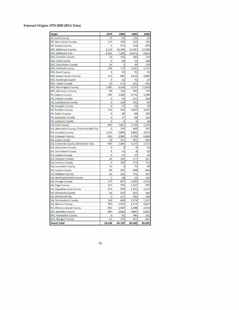
Regional E-I Travel Growth The TPB region and its surrounding areas have experienced significant housing and job growth over the past few decades; with that growth there has been a corresponding increase in external travel. VHB reviewed the BEA JTW data from 1970, 1980, and 1990 and compared them to the year 2000 data to reveal any changes in regional E-I travel patterns over time.8 The same post-processing steps applied to the year 2000 data were applied to the older data to ensure comparability. The external commuter sheds for the years 1970, 1980, 1990, and 2000 based on the BEA JTW data are depicted in Figure 4, Figure 5, Figure 6, and Figure 7, respectively. As mentioned previously, the BEA 2000 data differs slightly from the CTPP 2000 data, and some suppression was in place at the residential counties with few trips in the area to ensure confidentiality. Ultimately, the BEA 2000 JTW data are used here to provide a better comparison over time. In addition to the maps, tables of county-to-county flows for each year in the series and summaries for origins and destinations arrayed by year are contained in the appendix to this memo. As shown in Table 4, each state has grown at different levels in E-I travel between 1970 and 2000, with the highest percent growth occurring between 1970 and 1980 when total E-I trips more than doubled. The overall increase in external travel is 124% in 1970-1980, 84% in 1980-1990, and 24% in 1990-2000. The corresponding Compound Annual Growth Rate (CAGR) for each decade is eight, six, and two percent, respectively. Thus, the rate of growth in E-I travel has gone down over time.

7 Both BEA and the Census Bureau are part of the United States Department of Commerce. 8 Note that in earlier decades more of these trips would be considered E-I when compared with today, as the TPB modeled region has expanded over time.

12


13


14


15

Table 4: Regional External Travel Change from 1970 to 2000 (BEA)

Figures 8 through 10 show the change in external trips by jurisdiction between 1970 and 2000 by ten-year increments, and the CAGRs for the same periods are shown by state of residence in Figure 11 and workplace in Figure 12. There was growth in almost every external jurisdiction except for Dorchester County in Maryland and Lancaster County in Virginia. However, these two counties have zero trips to the TPB region reported in the BEA 1980 data. The highest growth for external travel occurred in Baltimore County, Baltimore City, and Washington County in Maryland. Between 1970 and 1980, all residence states experienced significant annual growth in external commuters, most of who travelled to Maryland and Virginia to work. Between 1980 and 1990, Pennsylvania, the Virginia external counties, and West Virginia continued to experience rapid growth. In terms of the destinations for those external travelers, Virginia and West Virginia had higher growth during this time. Between 1990 and 2000, Delaware had the highest percent growth but the overall number of external trips is just over 1,000, most of them from Sussex County. All the other residence states had a moderate percent growth but much more significant in absolute terms. All of the employment destinations experienced similar growth during this time.

16

Figure 8: Change in External Commuter Shed for the TPB Region from Year 1970 to 1980

17


18


20

Figure 11: Compound Annual Growth Rate for States of Residence over Time

0.0%

2.0%

4.0%

6.0%

8.0%

10.0%

12.0%

14.0%

1970-1980 1980-1990 1990-2000

CAGR

Delaware Maryland (Outside TPB Region)

Pennsylvania Virginia (Outside TPB Region)

West Virginia

Figure 12 Compound Annual Growth Rate for States of Work over Time

0.0%

2.0%

4.0%

6.0%

8.0%

10.0%

12.0%

14.0%

1970-1980 1980-1990 1990-2000

CAGR

DC Maryland (Inside TPB Region)

Virginia (Inside TPB Region) West Virginia (Jefferson)

21

E-I Travel and Comparable Regions to TPB The Federal Highway Administration report “Journey to Work in the United States and its Major Metropolitan Areas” presents the changes in terms of national and regional population and workforce, vehicle ownership, and travel to work characteristics that have occurred from 1960 to 2000 based on Census data. The following observations (many of them echoed in Pisarki’s CIA reports, based on the same datasets) were listed in the report:

• Family structure has changed over the years. In 1960, 52 percent of the family consisted of married couples with children while in 2000, there were only 35 percent. Average household size declined more than one-fifth, from 3.3 persons per household in 1960 to 2.6 in 2000.

• The increase of women in the workforce has resulted in the rise in household income and household auto ownership. For instance, average number of vehicles per household went from just over 1.0 in 1990 to approximately 1.7 in 2000 (so, while household size may be going down, trips per household are increasing across all trip purposes and major origin-destination categories, including E-I trips).

• Metropolitan Statistical Areas (MSAs) continue to grow in both area and population. Most of the population growth in the major metropolitan areas has occurred in the suburban counties (depending on how these counties are treated in MPO models, this growth results in increased I-I and / or E-I trips).

• The choice of a private vehicle as the primary transportation mode to work has increased, among which driving alone continued to increase as carpools continued to drop.

• The percent of workers with a long commute has increased. In 2000, 14 percent of commuters traveled more than 45 minutes compared to 12 percent in 1990. At the same time, 29 percent of commuters traveled less than 15 minutes compared to 31 percent in 1990. In 2000, more families are living and working in the suburbs. Workers in major MSAs are commuting 45 and even 60 minutes (or more) one way to their jobs on a regular basis. As noted previously, in 2000, the top three MSAs with the longest average travel time were New York, Washington D.C., and Atlanta.

• The 2000 Census shows a significant increase in travel time in all MSAs, which may give workers incentive for considering other modes, changing work times, or telecommuting.

Although the report provides some information before 1990, the analysis focuses on demographics and worker flow changes, specifically the growth in suburban commuting,9 from 1990 to 2000 for several large MSAs including Washington, D.C. and others that are comparable (see Table 5). Atlanta has a more detailed analysis and a longer time frame since it was selected as one of the case studies in the report. The San Francisco CMSA is similar to the TPB region in terms of both demographics and mode to work. The New York and Los Angeles CMSAs have much higher population, households, and workers, almost double or triple what the Washington D.C. CMSA has while the demographic data in the Atlanta CMSA are approximately half of those in the Washington area. Among the five CMSAs, the Washington D.C. MSA ranks number one in terms of workers per person and number four in terms of vehicles per household. The New York CMSA has the highest transit mode share and the lowest vehicles per household.

9 Suburban counties in the FHWA report are different from the external counties in the previous sections. Also, the MSAs are different (usually larger) from the regional modeled areas.

Comment [RIR1]: Maggie, please organize all the data referenced in this for each MSA into a matrix / table for quick comparison across areas and data elements and then have 1-2 paragraphs highlighting the similarities and differences compared to the TPB region

22

Table 5: Comparison of Journey to Work Profiles

Journey to Work Profile

New York-Northern New

Jersey-Long Island (NY-NJ-CT-PA CMSA)

Washington-Baltimore, DC-

MD-VA-WV CMSA

Los Angeles-Riverside-

Orange County, CA

CMSA

San Francisco-Oakland-San

Jose, CA CMSA

Atlanta, GA MSA

1990 19,549,649 6,727,050 14,531,529 6,253,311 2,959,950 Tot. Population 2000 21,199,865 7,608,070 16,373,645 7,039,362 4,112,198

1990 7,158,586 2,491,041 4,900,720 2,329,808 1,102,578 Tot. Households 2000 7,735,264 2,871,861 5,347,107 2,557,158 1,504,871

1990 9,271,089 3,611,094 6,809,043 3,200,833 1,542,948 Tot. Workers

2000 9,319,218 3,839,052 6,767,619 3,432,157 2,060,632

1990 0.47 0.54 0.47 0.51 0.52 Workers per Person 2000 0.44 0.50 0.41 0.49 0.50

1990 1.27 1.66 1.77 1.76 1.83 Vehicles per Household 2000 1.26 1.66 1.71 1.76 1.80

Mode to Work

2000 Drove alone (57%), Transit (25%), Carpool (9%), Work at

home (3%), Other (6%)

Drove Alone (71%), Carpool (13%), Transit (9%), Work at


Drove Alone (72%), Carpool (15%), Transit (5%), Work at


Drove alone (69%), Carpool (13%), Transit (9%), Work at


Drove alone (75%), Carpool (14%), Transit (3%), Work at


The New York-Northern New Jersey-Long Island (NY-NJ-CT-PA CMSA) grew approximately 8.4 percent total population between 1990 and 2000. The corresponding percent change in population in the central counties and suburban counties are 3.3 and 8.9, respectively. The growth of both population and households in the 1990s far outpaced the growth of total workers, which was approximately 0.5 percent. The number of workers with commuting time longer than 30 minutes has increased in the 1990s. The analysis on place of work and commuting flows for New York was not included in the report due to the difficulties of reconciling geographic definitions over time. The Washington-Baltimore, DC-MD-VA-WV CMSA has experienced population growth from 6.7 million in 1990 to 7.6 million in 2000, approximately 13.1 percent. Unlike New York, the central jurisdiction of Washington, D.C. had a decline of 5.7 percent in population while the suburban counties had a growth of 15.0 percent in the 1990s. The growth of households and workers from 1990 to 2000 was 15.3 percent and 6.3 percent, respectively. The number of workers with commuting time longer than 45 minutes has increased in the 1990s. There was a significant increase for the workers with more than a 60 minute commute. The analysis on journey-to-work data reveals that there was a decrease in the number of workers who live inside the MSA and work in the central city between 1990 and 2000. At the same time, there was a growth in terms of suburban internal and central-to-suburban county work flow.

23

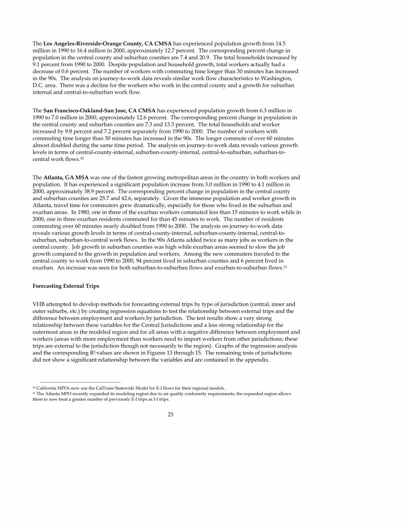
The Los Angeles-Riverside-Orange County, CA CMSA has experienced population growth from 14.5 million in 1990 to 16.4 million in 2000, approximately 12.7 percent. The corresponding percent change in population in the central county and suburban counties are 7.4 and 20.9. The total households increased by 9.1 percent from 1990 to 2000. Despite population and household growth, total workers actually had a decrease of 0.6 percent. The number of workers with commuting time longer than 30 minutes has increased in the 90s. The analysis on journey-to-work data reveals similar work flow characteristics to Washington, D.C. area. There was a decline for the workers who work in the central county and a growth for suburban internal and central-to-suburban work flow. The San Francisco-Oakland-San Jose, CA CMSA has experienced population growth from 6.3 million in 1990 to 7.0 million in 2000, approximately 12.6 percent. The corresponding percent change in population in the central county and suburban counties are 7.3 and 13.3 percent. The total households and worker increased by 9.8 percent and 7.2 percent separately from 1990 to 2000. The number of workers with commuting time longer than 30 minutes has increased in the 90s. The longer commute of over 60 minutes almost doubled during the same time period. The analysis on journey-to-work data reveals various growth levels in terms of central-county-internal, suburban-county-internal, central-to-suburban, suburban-to-central work flows.10 The Atlanta, GA MSA was one of the fastest growing metropolitan areas in the country in both workers and population. It has experienced a significant population increase from 3.0 million in 1990 to 4.1 million in 2000, approximately 38.9 percent. The corresponding percent change in population in the central county and suburban counties are 25.7 and 42.6, separately. Given the immense population and worker growth in Atlanta, travel time for commuters grew dramatically, especially for those who lived in the suburban and exurban areas. In 1980, one in three of the exurban workers commuted less than 15 minutes to work while in 2000, one in three exurban residents commuted for than 45 minutes to work. The number of residents commuting over 60 minutes nearly doubled from 1990 to 2000. The analysis on journey-to-work data reveals various growth levels in terms of central-county-internal, suburban-county-internal, central-to-suburban, suburban-to-central work flows. In the 90s Atlanta added twice as many jobs as workers in the central county. Job growth in suburban counties was high while exurban areas seemed to slow the job growth compared to the growth in population and workers. Among the new commuters traveled to the central county to work from 1990 to 2000, 94 percent lived in suburban counties and 6 percent lived in exurban. An increase was seen for both suburban-to-suburban flows and exurban-to-suburban flows.11 Forecasting External Trips VHB attempted to develop methods for forecasting external trips by type of jurisdiction (central, inner and outer suburbs, etc.) by creating regression equations to test the relationship between external trips and the difference between employment and workers by jurisdiction. The test results show a very strong relationship between these variables for the Central Jurisdictions and a less strong relationship for the outermost areas in the modeled region and for all areas with a negative difference between employment and workers (areas with more employment than workers need to import workers from other jurisdictions; these trips are external to the jurisdiction though not necessarily to the region). Graphs of the regression analysis and the corresponding R2 values are shown in Figures 13 through 15. The remaining tests of jurisdictions did not show a significant relationship between the variables and are contained in the appendix.

10 California MPOs now use the CalTrans Statewide Model for E-I flows for their regional models. 11 The Atlanta MPO recently expanded its modeling region due to air quality conformity requirements; the expanded region allows them to now treat a greater number of previously E-I trips as I-I trips.

24

Figure 13: Regression of Number of External Trips vs. (Employment minus Workers) – Central Jurisdictions

y = 0.0257x + 366.32R² = 0.9597

0

2,000

4,000

6,000

8,000

10,000

12,000

14,000

-50,000 0 50,000 100,000 150,000 200,000 250,000 300,000 350,000 400,000 450,000

Exte

rnal

Trav

el

Difference between Employment and Workers

Figure 14: Regression of Number of External Trips vs. (Employment minus Workers) for Modeled Region – Fredericksburg Area Jurisdictions and Other Jurisdictions

y = -0.2207x + 1606.2R² = 0.6852

-1,000

0

1,000

2,000

3,000

4,000

5,000

6,000

-15,000 -10,000 -5,000 0 5,000 10,000

Exte

rnal

Trav

el


25

Figure 15: Regression of Number of External Trips vs. (Employment minus Workers) for areas with Negative Values of (Employment minus Workers) (Excluding Outliers)

Implications for TPB Modeling Process The impacts on travel demand forecasting and regional transportation planning as exurban growth patterns continue to fuel larger numbers of extreme commuters are significant (pun intended). Based on our regression analysis, several predictive equations for forecasting external trips in certain areas are contained in this memo. Many references have been made in the literature to the trade-offs between the social and time costs of long-distance commuting and the corresponding decrease in housing costs by moving farther away from a region’s central jurisdictions. However, most of the traveler behavior considered by previous studies took place under (relatively) inexpensive gasoline (i.e., less than $2.50 per gallon for “regular” unleaded self-serve). The current actual price of gasoline nationally and regionally is now well beyond any of the forecast values contained in MPO models, and the most recent research is focusing on the elasticity of gas prices with regards to auto travel of all purposes and distances.12 There are early Federal reports of decreased VMT nationally, but there are not enough data to consider future trends. It does seem likely that a continued increase in gas prices will eventually temper the growth in E-I trips, but much is dependent on the impact across different economic strata, something which should be addressed by further testing. One other potential area for further analysis would be backcasting using some of the predictive equations, the historical BEA data, and the actual boundaries of the TPB modeled region for 1970, 1980, and 1990 to see how well E-I travel was forecast in the past under previous models, as well as the effect of expanding the model boundary. For example, when Frederick County was added to the TPB region one possible effect may have been increased model sensitivity to and capture of “new” E-I trips from Washington County into the TPB region. CIA III notes that detailed JTW analysis will become more challenging in the near future as some historical elements of the decennial CTPP data are replaced by the ACS and urges local supplemental data collection (and funding to support it). VHB echoes this call for more data, as the nature of E-I travel in the region will

12 Recent chatter on the TMIP listserv has referenced a January 2008 report by the Congressional Budget Office, reports from the Victoria Transport Policy Institute, and illustrated interest in this topic at the MPO, transit agency, and State DOT levels,

26

continue to change, dependent (or not) on changes in the price of gasoline. In the end, the TPB model must do a reasonable job at predicting this (for now) growing regional travel market.

References D. Cohn and R. Samuels. “Daily Misery Has a Number: Commute 2nd Longest in U.S.” The Washington Post, 6/30/2006. R.Cervero, K. Chapple, J. Landis, and M. Wachs. Making Do: How Working Families in Seven U.S. Metropolitan Areas Trade Off Housing Costs and Commuting Times. Berkeley, CA, June 2006. Conlin, M., Gard, L., Doyle, R., and M. Arndt. “Extreme Commuting,” Business Week, 2/21/2005. http://www.businessweek.com/magazine/content/05_08/b3921127.htm A. MacGills. “Ties to Far-Flung Homes Drive Commuters to Great Lengths.” The Washington Post, 4/25/2006. E. Weiss. “Va., Md. Top List for Percentage of Out-of-County Commutes.” The Washington Post, 10/17/2006. Howlett, D. and P. Overberg. “Think Your Commute is Tough?” USA Today, 11/29/2004. http://www.usatoday.com/news/nation/2004-11-29-commute_x.htm L. Smith, “Extreme Commuting: Is It For You?” Forbes Media Company, 2006. http://www.investopedia.com/articles/pf/06/extremecommute.asp L. Rowley, “Commuting is a Drag (on the Economy). Yahoo! Finance, 7/27/2006. http://finance.yahoo.com/expert/article/moneyhappy/7928 N. Paumgarten. “Annals of Transport: There and Back Again, the Soul of the Commuter.” The New Yorker, 4/16/2007. http://www.newyorker.com/reporting/2007/04/16/070416fa_fact_paumgarten A. Murray. “The Commuters of Easton.” All Things Considered, National Public Radio, 7/5/2006. http://www.npr.org/templates/story/story.php?storyId=5536306 J. Bailey. “Extreme Commutes Grow Longer in Air Industry.” The New York Times, 6/11/2006. http://www.nytimes.com/2006/06/11/business/11commute.html?_r=1&oref=slogin D. Terry. Subdivided: Isolation & Community in America, 2007 film. Film website and accompaning blog and other features at http://subdivided.net/ P. Jonsson. “Americans Adapt Creatively to Long Commutes.” The Christian Science Monitor, 9/19/2007. http://www.csmonitor.com/2007/0919/p01s01-ussc.html Nancy, M. and S. Nanda. “Journey to Work Trends in the United States and its Major Metropolitan Area” 06/30/2003. http://www.fhwa.dot.gov/ctpp/jtw/index.htm

27

Appendix

28

Jurisdiction Types: TPB Modeled Region

Central Jurisdictions District of Columbia, Arlington County, City of Alexandria

Inner Suburbs Montgomery County, Prince George’s County, Fairfax County, City of Fairfax, City of Falls Church

Outer Suburbs Loudoun County, Prince William County, City of Manassas, City of Manassas Park, Calvert County, Charles County, Frederick County, Stafford County

Modeled Region – Baltimore Area Jurisdictions

Anne Arundel County, Carroll County, Howard County

Modeled Region – Fredericksburg Area Jurisdictions

King George County, Spotsylvania County (Modeled Portion Only), Fredericksburg City

Modeled Region – Other Jurisdictions St. Mary’s County, Clarke County, Fauquier County, Jefferson County

29

Regression of Number of External Trips vs. (Employment minus Workers) -- TPB Latest Modeled Region without Baltimore Area

y = 0.017x + 3870.2R² = 0.194

0

2,000

4,000

6,000

8,000

10,000

12,000

14,000

-200,000 -100,000 0 100,000 200,000 300,000 400,000 500,000

Exte

rnal

Trav

el


Regression of Number of External Trips vs. (Employment minus Workers) -- Suburban Jurisdictions

30

Regression of Number of External Trips vs. (Employment minus Workers) for areas with Positive Values for (Employment minus Workers)

y = 0.0172x + 4272.4R² = 0.2565

0

2,000

4,000

6,000

8,000

10,000

12,000

14,000

0 50,000 100,000 150,000 200,000 250,000 300,000 350,000 400,000 450,000

Exte

rnal

Trav

el


31

Historical Employment and Household Data for TPB Region

Notes: Employment and household data were provided by MWCOG; 1980 data were from Round 3.5 - 1985 Update; 1990 data were from Round 5.1 - May 1994; 2000 data were from Round 7.0a - Oct 2006; Workers per household data were obtained from Journey to Work Trends report; External travel data were derived from BEA data.

32

County to County Flows (After Post-Processing)

33

External Origins 1970-2000 (BEA Data)

34

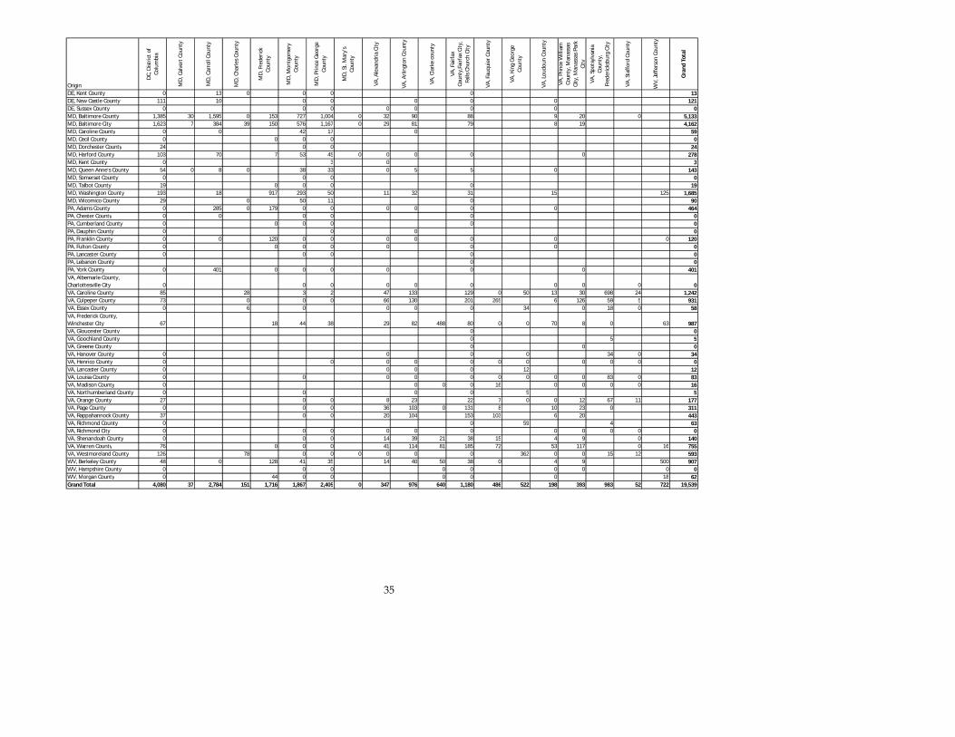
Year 1970 County-to-County Flow (BEA JTW Data)

35

Origin

DC, D

istric

t of

Colu

mbi

a

MD,

Cal

vert

Cou

nty

MD,

Car

roll

Coun

ty

MD,

Cha

rles C

ount

y

MD,

Fre

deric

k Co

unty

MD,

Mon

tgom

ery

Coun

ty

MD,

Prin

ce G

eorg

e Co

unty

MD,

St.

Mar

y's

Coun

ty

VA, A

lexa

ndria

City

VA, A

rling

ton

Coun

ty

VA, C

lark

e co

unty

VA, F

airfa

x Co

unty

,Fai

rfax C

ity,

Falls

Chu

rch

City

VA, F

auqu

ier C

ount

y

VA, K

ing

Geor

ge

Coun

ty

VA, L

oudo

un C

ount

y

VA, P

rince

Will

iam

Co

unty

, Man

assa

s Ci

ty, M

anas

sas P

ark

City

VA, S

pots

ylva

nia

Coun

ty,

Fred

erick

sbur

g Ci

ty

VA, S

taffo

rd C

ount

y

WV,

Jeffe

rson

Cou

nty

Gran

d To

tal

DE, Kent County 0 13 0 0 0 0 13DE, New Castle County 111 10 0 0 0 0 0 121DE, Sussex County 0 0 0 0 0 0 0 0MD, Baltimore County 1,385 30 1,595 0 153 727 1,004 0 32 90 88 9 20 0 5,133MD, Baltimore City 1,623 7 384 39 150 576 1,167 0 29 81 79 8 19 4,162MD, Caroline County 0 0 42 17 0 59MD, Cecil County 0 0 0 0 0MD, Dorchester County 24 0 0 24MD, Harford County 103 70 7 53 45 0 0 0 0 0 278MD, Kent County 0 3 0 3MD, Queen Anne's County 54 0 8 0 38 33 0 5 5 0 143MD, Somerset County 0 0 0 0MD, Talbot County 19 0 0 0 0 19MD, Washington County 193 18 917 293 50 11 32 31 15 125 1,685MD, Wicomico County 29 0 50 11 0 90PA, Adams County 0 285 0 179 0 0 0 0 0 0 464PA, Chester County 0 0 0 0 0 0PA, Cumberland County 0 0 0 0 0 0PA, Dauphin County 0 0 0 0PA, Franklin County 0 0 120 0 0 0 0 0 0 0 120PA, Fulton County 0 0 0 0 0 0 0 0PA, Lancaster County 0 0 0 0 0PA, Lebanon County 0 0PA, York County 0 401 0 0 0 0 0 0 401VA, Albemarle County, Charlottesville City 0 0 0 0 0 0 0 0 0 0VA, Caroline County 85 28 3 2 47 133 129 0 50 13 30 698 24 1,242VA, Culpeper County 73 0 0 0 66 130 201 265 6 126 59 5 931VA, Essex County 0 6 0 0 0 0 34 0 18 0 58VA, Frederick County, Winchester City 67 18 44 38 29 82 488 80 0 0 70 8 0 63 987VA, Gloucester County 0 0VA, Goochland County 0 5 5VA, Greene County 0 0 0VA, Hanover County 0 0 0 0 34 0 34VA, Henrico County 0 0 0 0 0 0 0 0 0 0 0VA, Lancaster County 0 0 0 0 12 12VA, Louisa County 0 0 0 0 0 0 0 0 0 83 0 83VA, Madison County 0 0 0 0 16 0 0 0 0 16VA, Northumberland County 0 0 0 0 5 5VA, Orange County 27 0 0 8 23 22 7 0 0 12 67 11 177VA, Page County 0 0 0 36 103 0 131 8 10 23 0 311VA, Rappahannock County 37 0 0 20 104 153 103 6 20 443VA, Richmond County 0 0 59 4 63VA, Richmond City 0 0 0 0 0 0 0 0 0 0 0VA, Shenandoah County 0 0 0 14 39 21 38 15 4 9 0 140VA, Warren County 76 0 0 0 41 114 81 185 72 53 117 0 16 755VA, Westmoreland County 126 78 0 0 0 0 0 0 362 0 0 15 12 593WV, Berkeley County 48 0 128 41 35 14 40 50 38 0 4 9 500 907WV, Hampshire County 0 0 0 0 0 0 0 0 0WV, Morgan County 0 44 0 0 0 0 0 18 62Grand Total 4,080 37 2,784 151 1,716 1,867 2,405 0 347 976 640 1,180 486 522 198 393 983 52 722 19,539

36


Origin

DC, D

istric

t of

Colu

mbi

a

MD,

Cal

vert

Cou

nty

MD,

Car

roll

Coun

ty

MD,

Cha

rles C

ount

y

MD,

Fre

deric

k Co

unty

MD,

Mon

tgom

ery

Coun

ty

MD,

Prin

ce G

eorg

e Co

unty

MD,

St.

Mar

y's

Coun

ty

VA, A

lexa

ndria

City

VA, A

rling

ton

Coun

ty

VA, C

lark

e co

unty

VA, F

airfa

x Co

unty

,Fai

rfax C

ity,

Falls

Chu

rch

City

VA, F

auqu

ier C

ount

y

VA, K

ing

Geor

ge

Coun

ty

VA, L

oudo

un C

ount

y

VA, P

rince

Will

iam

Co

unty

, Man

assa

s Ci

ty, M

anas

sas P

ark

City

VA, S

pots

ylva

nia

Coun

ty,

Fred

erick

sbur

g Ci

ty

VA, S

taffo

rd C

ount

y

WV,

Jeffe

rson

Cou

nty

Gran

d To

tal

DE, Kent County 35 0 0 52 12 0 99DE, New Castle County 63 0 26 41 14 43 0 187DE, Sussex County 39 0 100 0 0 32 0 171MD, Baltimore County 1,849 36 2,644 57 182 1,470 4,352 36 50 330 382 8 0 0 11,396MD, Baltimore City 2,489 0 574 53 83 808 2,873 46 51 147 134 25 0 7,283MD, Caroline County 8 0 36 95 0 139MD, Cecil County 0 0 0 28 28MD, Dorchester County 0 0 0 0MD, Harford County 184 105 0 57 254 0 14 107 51 0 772MD, Kent County 0 9 24 33MD, Queen Anne's County 207 0 0 15 56 321 0 12 50 0 661MD, Somerset County 0 43 9 52MD, Talbot County 60 0 49 55 9 173MD, Washington County 276 18 2,564 971 112 14 10 182 29 128 4,304MD, Wicomico County 14 11 29 45 27 126PA, Adams County 48 617 0 305 101 83 0 0 31 0 1,185PA, Chester County 24 0 0 0 16 40PA, Cumberland County 74 0 53 4 33 164PA, Dauphin County 32 0 0 32PA, Franklin County 35 23 226 12 17 0 13 0 0 0 326PA, Fulton County 0 26 2 0 0 0 0 28PA, Lancaster County 0 0 0 47 47PA, Lebanon County 0 0PA, York County 43 882 18 42 58 0 18 0 1,061VA, Albemarle County, Charlottesville City 15 0 32 13 11 7 0 27 0 105VA, Caroline County 156 0 36 26 87 26 213 0 199 0 49 986 106 1,884VA, Culpeper County 170 0 36 0 11 115 589 748 14 291 87 21 2,082VA, Essex County 11 43 0 24 28 69 93 0 39 0 307VA, Frederick County, Winchester City 95 29 64 12 32 36 1,396 315 86 0 276 45 12 51 2,449VA, Gloucester County 0 0VA, Goochland County 0 43 43VA, Greene County 46 21 67VA, Hanover County 0 0 28 0 55 17 100VA, Henrico County 37 36 0 49 11 0 0 0 109 0 242VA, Lancaster County 0 0 0 0 0 0VA, Louisa County 76 0 0 0 44 0 0 0 23 108 0 251VA, Madison County 13 0 0 40 18 0 45 0 0 116VA, Northumberland County 0 0 0 0 38 38VA, Orange County 57 0 28 38 39 75 93 11 0 84 459 13 897VA, Page County 56 34 37 40 59 0 370 64 3 76 0 739VA, Rappahannock County 36 0 0 42 13 201 263 13 7 575VA, Richmond County 6 0 113 24 143VA, Richmond City 66 32 0 22 0 19 0 0 78 0 217VA, Shenandoah County 88 0 19 44 0 10 277 14 6 8 0 466VA, Warren County 164 0 12 7 22 43 85 673 167 106 231 0 0 1,510VA, Westmoreland County 128 56 52 0 0 17 11 71 538 0 0 144 12 1,029WV, Berkeley County 184 0 186 154 35 27 0 53 61 0 52 0 1,067 1,819WV, Hampshire County 20 0 0 32 25 0 4 0 81WV, Morgan County 53 78 27 36 27 19 13 0 253Grand Total 6,911 36 4,863 235 3,697 4,254 8,736 82 572 1,063 1,603 4,208 1,453 992 545 911 2,144 169 1,246 43,720

37


Origin

DC, D

istric

t of

Colu

mbi

a

MD,

Cal

vert

Cou

nty

MD,

Car

roll

Coun

ty

MD,

Cha

rles C

ount

y

MD,

Fre

deric

k Co

unty

MD,

Mon

tgom

ery

Coun

ty

MD,

Prin

ce G

eorg

e Co

unty

MD,

St.

Mar

y's

Coun

ty

VA, A

lexa

ndria

City

VA, A

rling

ton

Coun

ty

VA, C

lark

e co

unty

VA, F

airfa

x Co

unty

,Fai

rfax C

ity,

Falls

Chu

rch

City

VA, F

auqu

ier C

ount

y

VA, K

ing

Geor

ge

Coun

ty

VA, L

oudo

un C

ount

y

VA, P

rince

Will

iam

Co

unty

, Man

assa

s Ci

ty, M

anas

sas P

ark

City

VA, S

pots

ylva

nia

Coun

ty,

Fred

erick

sbur

g Ci

ty

VA, S

taffo

rd C

ount

y

WV,

Jeffe

rson

Cou

nty

Gran

d To

tal

DE, Kent County 43 0 20 14 28 21 126DE, New Castle County 126 0 56 14 29 8 0 233DE, Sussex County 36 21 10 0 33 15 0 115MD, Baltimore County 2,782 9 3,059 68 257 2,466 3,926 21 214 290 599 73 23 0 13,787MD, Baltimore City 3,170 59 886 56 92 1,797 3,747 18 154 381 465 0 51 10,876MD, Caroline County 35 0 21 130 0 186MD, Cecil County 0 0 0 41 41MD, Dorchester County 20 0 0 20MD, Harford County 361 263 42 266 344 0 28 78 138 21 1,541MD, Kent County 0 45 7 52MD, Queen Anne's County 433 29 0 26 188 723 0 77 56 0 1,532MD, Somerset County 0 2 43 45MD, Talbot County 94 0 52 75 44 265MD, Washington County 561 90 5,189 2,570 194 20 37 280 174 242 9,357MD, Wicomico County 33 25 42 166 17 283PA, Adams County 106 1,246 0 949 317 71 0 0 59 25 2,773PA, Chester County 67 0 47 0 39 153PA, Cumberland County 49 0 19 20 53 141PA, Dauphin County 28 0 0 28PA, Franklin County 133 90 1,063 336 51 0 22 122 39 41 1,897PA, Fulton County 0 60 38 0 0 0 0 98PA, Lancaster County 0 34 25 9 68PA, Lebanon County 0 0PA, York County 96 1,180 85 115 172 0 80 0 1,728VA, Albemarle County, Charlottesville City 136 25 11 28 37 61 20 56 26 400VA, Caroline County 239 28 4 23 35 96 183 0 207 38 154 1,579 306 2,892VA, Culpeper County 247 0 110 0 49 72 1,483 1,646 197 669 203 123 4,799VA, Essex County 31 30 22 18 63 115 97 0 85 30 491VA, Frederick County, Winchester City 190 18 143 37 29 130 1,211 1,618 195 0 1,213 292 26 120 5,222VA, Gloucester County 0 0VA, Goochland County 0 8 8VA, Greene County 15 2 17VA, Hanover County 22 20 9 20 79 27 177VA, Henrico County 95 18 0 45 143 0 39 37 149 27 553VA, Lancaster County 47 0 0 26 0 73VA, Louisa County 13 50 0 31 115 0 0 0 76 267 56 608VA, Madison County 106 21 21 130 113 0 84 0 0 475VA, Northumberland County 27 0 0 34 0 61VA, Orange County 149 0 30 98 106 335 121 45 26 183 745 211 2,049VA, Page County 102 98 88 21 54 0 386 95 34 187 37 1,102VA, Rappahannock County 79 0 21 27 58 415 495 71 275 1,441VA, Richmond County 30 0 86 39 155VA, Richmond City 85 23 0 31 33 82 20 33 89 0 396VA, Shenandoah County 116 52 87 44 65 31 514 60 177 206 22 1,374VA, Warren County 305 0 123 80 68 154 91 1,896 333 378 1,284 0 0 4,712VA, Westmoreland County 270 112 21 82 0 64 57 174 1,249 20 0 234 85 2,368WV, Berkeley County 305 25 567 576 90 56 71 187 323 0 421 105 2,161 4,887WV, Hampshire County 50 0 35 65 99 45 52 0 346WV, Morgan County 70 57 83 11 24 80 41 65 431Grand Total 10,887 97 6,839 365 8,379 9,731 10,438 39 1,011 2,040 1,630 10,241 3,058 1,743 3,012 3,790 3,540 913 2,629 80,382

38


Origin

DC, D

istric

t of

Colu

mbi

a

MD,

Cal

vert

Cou

nty

MD,

Car

roll

Coun

ty

MD,

Cha

rles C

ount

y

MD,

Fre

deric

k Co

unty

MD,

Mon

tgom

ery

Coun

ty

MD,

Prin

ce G

eorg

e Co

unty

MD,

St.

Mar

y's

Coun

ty

VA, A

lexa

ndria

City

VA, A

rling

ton

Coun

ty

VA, C

lark

e co

unty

VA, F

airfa

x Co

unty

,Fai

rfax C

ity,

Falls

Chu

rch

City

VA, F

auqu

ier C

ount

y

VA, K

ing

Geor

ge

Coun

ty

VA, L

oudo

un C

ount

y

VA, P

rince

Will

iam

Co

unty

, Man

assa

s Ci

ty, M

anas

sas P

ark

City

VA, S

pots

ylva

nia

Coun

ty,

Fred

erick

sbur

g Ci

ty

VA, S

taffo

rd C

ount

y

WV,

Jeffe

rson

Cou

nty

Gran

d To

tal

DE, Kent County 43 0 0 0 20 0 63DE, New Castle County 87 0 24 58 38 65 19 291DE, Sussex County 132 112 151 44 54 148 29 670MD, Baltimore County 3,668 60 3,875 95 550 2,990 4,715 22 94 440 757 155 35 50 17,506MD, Baltimore City 3,040 0 965 90 113 1,760 2,915 0 204 249 410 45 30 9,821MD, Caroline County 96 19 0 131 12 258MD, Cecil County 29 38 22 29 118MD, Dorchester County 35 26 58 119MD, Harford County 465 319 16 330 695 39 34 99 154 0 2,151MD, Kent County 39 12 0 51MD, Queen Anne's County 775 0 22 18 309 1,200 33 72 135 39 2,603MD, Somerset County 24 0 0 24MD, Talbot County 175 18 73 149 28 443MD, Washington County 474 161 7,150 2,355 254 48 74 284 264 394 11,458MD, Wicomico County 42 0 45 42 0 129PA, Adams County 100 1,865 20 1,725 314 51 12 22 63 27 4,199PA, Chester County 14 19 41 44 38 156PA, Cumberland County 0 34 29 8 23 94PA, Dauphin County 29 25 24 78PA, Franklin County 48 93 1,785 378 88 24 50 139 39 28 2,672PA, Fulton County 12 61 50 8 8 12 4 155PA, Lancaster County 28 65 0 39 132PA, Lebanon County 28 28PA, York County 97 1,815 195 42 123 34 0 18 2,324VA, Albemarle County, Charlottesville City 180 0 0 0 0 67 0 0 0 247VA, Caroline County 218 0 32 26 24 54 225 19 263 0 173 1,963 574 3,571VA, Culpeper County 260 30 63 49 123 149 1,820 2,055 197 992 332 210 6,280VA, Essex County 32 0 0 0 12 56 110 20 132 42 404VA, Frederick County, Winchester City 284 71 201 26 76 80 1,507 1,900 234 20 2,074 540 0 199 7,212VA, Gloucester County 44 44VA, Goochland County 38 14 52VA, Greene County 0 35 35VA, Hanover County 53 0 80 55 141 38 367VA, Henrico County 159 34 24 88 194 25 34 59 96 40 753VA, Lancaster County 24 28 18 28 0 98VA, Louisa County 100 39 25 44 194 12 15 22 56 277 64 848VA, Madison County 0 65 0 105 119 20 100 84 14 507VA, Northumberland County 24 44 30 37 25 160VA, Orange County 163 63 19 99 95 310 183 35 48 220 1,310 375 2,920VA, Page County 123 34 18 33 8 20 392 79 94 160 14 975VA, Rappahannock County 113 18 44 34 35 316 513 93 268 1,434VA, Richmond County 22 33 50 0 105VA, Richmond City 115 0 54 0 44 124 0 55 73 35 500VA, Shenandoah County 112 44 26 29 69 98 486 77 188 158 0 1,287VA, Warren County 368 38 132 83 57 158 204 2,497 500 689 1,067 19 30 5,842VA, Westmoreland County 199 130 0 139 12 53 32 272 960 22 68 412 237 2,536WV, Berkeley County 499 25 1,075 465 64 0 85 340 369 39 605 110 3,154 6,830WV, Hampshire County 44 39 0 28 91 72 0 18 292WV, Morgan County 49 77 59 54 48 14 18 144 463Grand Total 12,593 60 9,178 383 12,946 10,198 11,412 73 1,140 2,200 2,245 12,015 3,855 1,567 4,763 4,164 4,848 1,698 3,967 99,305

fy08 pt3 exurban travel reformatted - home - ampo covering exurban commuters and analysis of census...

Documents