fuzzy systems - fuzzy control - is.ovgu.defuzzy+sets/fs_part03_control.pdf · logic fuzzy...
TRANSCRIPT

Fuzzy SystemsFuzzy Control
Prof. Dr. Rudolf Kruse Alexander Dockhorn{kruse,dockhorn}@ovgu.de
Otto-von-Guericke University of MagdeburgFaculty of Computer Science
Institute of Intelligent Cooperating Systems
R. Kruse, A. Dockhorn FS – Fuzzy Control Part 3 1 / 59

Mamdani Control

Architecture of a Fuzzy Controller
controlledsystem
measuredvalues
controlleroutput
notfuzzy
notfuzzy
fuzzificationinterface fuzzy
decisionlogic fuzzy
defuzzificationinterface
knowledgebase
R. Kruse, A. Dockhorn FS – Fuzzy Control Part 3 2 / 59

Example: Cartpole Problem (cont.)
X1 is partitioned into 7 fuzzy sets.
Support of fuzzy sets: intervals with length 14 of whole range X1.
Similar fuzzy partitions for X2 and Y .
Next step: specify rules
if ξ1 is A(1) and . . . and ξn is A(n) then η is B,
A(1), . . . , A(n) and B represent linguistic terms corresponding toµ(1), . . . , µ(n) and µ according to X1, . . . , Xn and Y .
Let the rule base consist of k rules.
R. Kruse, A. Dockhorn FS – Fuzzy Control Part 3 3 / 59
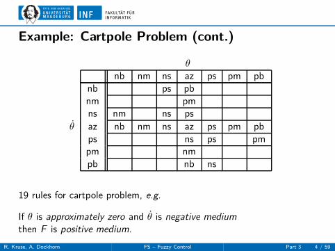
Example: Cartpole Problem (cont.)
θnb nm ns az ps pm pb
nb ps pbnm pmns nm ns ps
θ̇ az nb nm ns az ps pm pbps ns ps pmpm nmpb nb ns
19 rules for cartpole problem, e.g.
If θ is approximately zero and θ̇ is negative mediumthen F is positive medium.
R. Kruse, A. Dockhorn FS – Fuzzy Control Part 3 4 / 59

Definition of Table-based Control Function
Measurement (x1, . . . , xn) ∈ X1 × . . . × Xn is forwarded to decisionlogic.
Consider rule
if ξ1 is A(1) and . . . and ξn is A(n) then η is B.
Decision logic computes degree to ξ1, . . . , ξn fulfills premise of rule.
For 1 ≤ ν ≤ n, the value µ(ν)(xν) is calculated.
Combine values conjunctively by α = min{
µ(1), . . . , µ(n)}
.
For each rule Rr with 1 ≤ r ≤ k, compute
αr = min{
µ(1)i1,r
(x1), . . . , µ(n)in,r
(xn)}
.
R. Kruse, A. Dockhorn FS – Fuzzy Control Part 3 5 / 59
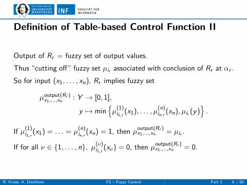
Definition of Table-based Control Function II
Output of Rr = fuzzy set of output values.
Thus “cutting off” fuzzy set µir associated with conclusion of Rr at αr .
So for input (x1, . . . , xn), Rr implies fuzzy set
µoutput(Rr )x1,...,xn
: Y → [0, 1],
y 7→ min{
µ(1)i1,r
(x1), . . . , µ(n)in,r
(xn), µir (y)}
.
If µ(1)i1,r
(x1) = . . . = µ(n)in,r
(xn) = 1, then µoutput(Rr )x1,...,xn = µir .
If for all ν ∈ {1, . . . , n}, µ(ν)i1,r
(xν) = 0, then µoutput(Rr )x1,...,xn = 0.
R. Kruse, A. Dockhorn FS – Fuzzy Control Part 3 6 / 59

Combination of Rules
The decision logic combines the fuzzy sets from all rules.
The maximum leads to the output fuzzy set
µoutputx1,...,xn
: Y → [0, 1],
y 7→ max1≤r≤k
{
min{
µ(1)i1,r
(x1), . . . , µ(n)in,r
(xn), µir (y)}}
.
Then µoutputx1,...,xn is passed to defuzzification interface.
R. Kruse, A. Dockhorn FS – Fuzzy Control Part 3 7 / 59

Rule Evaluation
θ0 15 25 30 45
1
θ0 15 25 30 45
1positive small
0.3
positive medium
0.6
min
min
θ̇−8 −4 0 8
0.5
1approx.zero
θ̇−8 −4 0 8
0.5
1approx.zero
F
1
F
1
F
1
0 3 6 9
0 3 6 9
positive small
positive medium
max
0 1 4 4.5 7.5 9
Rule evaluation for Mamdani-Assilian controller.
Input tuple (25, −4) leads to fuzzy output.
Crisp output is determined by defuzzification.
R. Kruse, A. Dockhorn FS – Fuzzy Control Part 3 8 / 59

Defuzzification
So far: mapping between each (n1, . . . , nn) and µoutputx1,...,xn .
Output = description of output value as fuzzy set.
Defuzzification interface derives crisp value from µoutputx1,...,xn .
This step is called defuzzification.
Most common methods:
• max criterion,
• mean of maxima,
• center of gravity.
R. Kruse, A. Dockhorn FS – Fuzzy Control Part 3 9 / 59

The Max Criterion Method
Choose an arbitrary y ∈ Y for which µoutputx1,...,xn reaches the maximum
membership value.
Advantages:
• Applicable for arbitrary fuzzy sets.
• Applicable for arbitrary domain Y (even for Y 6= IR).
Disadvantages:
• Rather class of defuzzification strategies than single method.
• Which value of maximum membership?
• Random values and thus non-deterministic controller.
• Leads to discontinuous control actions.
R. Kruse, A. Dockhorn FS – Fuzzy Control Part 3 10 / 59

The Mean of Maxima (MOM) Method
Preconditions:
(i) Y is interval
(ii) YMax = {y ∈ Y | ∀y ′ ∈ Y : µoutputx1,...,xn(y ′) ≤ µoutput
x1,...,xn(y)} isnon-empty and measurable
(iii) YMax is set of all y ∈ Y such that µoutputx1,...,xn is maximal
Crisp output value = mean value of YMax.
if YMax is finite:
η =1
|YMax|
∑
yi ∈YMax
yi
if YMax is infinite:
η =
∫
y∈YMaxy dy
∫
y∈YMaxdy
MOM can lead to discontinuous control actions.
R. Kruse, A. Dockhorn FS – Fuzzy Control Part 3 11 / 59
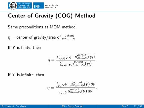
Center of Gravity (COG) Method
Same preconditions as MOM method.
η = center of gravity/area of µoutputx1,...,xn
If Y is finite, then
η =
∑
yi∈Y yi · µoutputx1,...,xn(yi )
∑
yi ∈Y µoutputx1,...,xn(yi)
.
If Y is infinite, then
η =
∫
y∈Y y · µoutputx1,...,xn(y) dy
∫
y∈Y µoutputx1,...,xn(y) dy
.
R. Kruse, A. Dockhorn FS – Fuzzy Control Part 3 12 / 59

Center of Gravity (COG) Method
Advantages:
• Nearly always smooth behavior,
• If certain rule dominates once, not necessarily dominating again.
Disadvantage:
• No semantic justification,
• Long computation,
• Counterintuitive results possible.
Also called center of area (COA) method :
take value that splits µoutputx1,...,xn into 2 equal parts.
R. Kruse, A. Dockhorn FS – Fuzzy Control Part 3 13 / 59
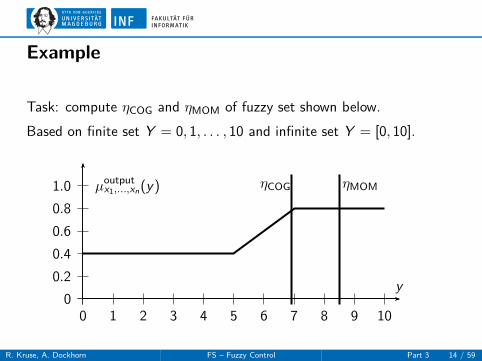
Example
Task: compute ηCOG and ηMOM of fuzzy set shown below.
Based on finite set Y = 0, 1, . . . , 10 and infinite set Y = [0, 10].
0 1 2 3 4 5 6 7 8 9 100
0.2
0.4
0.6
0.8
1.0 ηCOG ηMOMµoutputx1,...,xn(y)
y
R. Kruse, A. Dockhorn FS – Fuzzy Control Part 3 14 / 59

Example for COGContinuous and Discrete Output Space
ηCOG =
∫ 100 y · µoutput
x1,...,xn(y) dy∫ 10
0 µoutputx1,...,xn(y) dy
=
∫ 50 0.4y dy +
∫ 75 (0.2y − 0.6)y dy +
∫ 107 0.8y dy
5 · 0.4 + 2 · 0.8+0.42 + 3 · 0.8
≈38.7333
5.6≈ 6.917
ηCOG =0.4 · (0 + 1 + 2 + 3 + 4 + 5) + 0.6 · 6 + 0.8 · (7 + 8 + 9 + 10)
0.4 · 6 + 0.6 · 1 + 0.8 · 4
=36.8
6.2≈ 5.935
R. Kruse, A. Dockhorn FS – Fuzzy Control Part 3 15 / 59

Example for MOMContinuous and Discrete Output Space
ηMOM =
∫ 107 y dy∫ 10
7 dy
=50 − 24.5
10 − 7=
25.5
3
= 8.5
ηMOM =7 + 8 + 9 + 10
4
=34
4
= 8.5
R. Kruse, A. Dockhorn FS – Fuzzy Control Part 3 16 / 59

Problem Case for MOM and COG
−2 −1 0 1 20
1µoutput
x1,...,xn
What would be the output of MOM or COG?
Is this desirable or not?
R. Kruse, A. Dockhorn FS – Fuzzy Control Part 3 17 / 59

Example: Engine Idle Speed ControlVW 2000cc 116hp Motor (Golf GTI)
R. Kruse, A. Dockhorn FS – Fuzzy Control Part 3 18 / 59
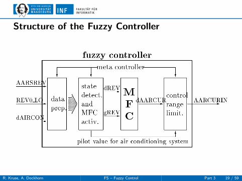
Structure of the Fuzzy Controller
R. Kruse, A. Dockhorn FS – Fuzzy Control Part 3 19 / 59

Deviation of the Number of RevolutionsdREV
−70 −50 −30 −10 10 30 50 700
0.25
0.50
0.75
1.00
nb nm ns zr ps pm pb
R. Kruse, A. Dockhorn FS – Fuzzy Control Part 3 20 / 59

Gradient of the Number of RevolutionsgREV
0
0.25
0.50
0.75
1.00
-400 -400-70 70-40 40-30 30-20 20
nb nm ns zr ps pm pb
R. Kruse, A. Dockhorn FS – Fuzzy Control Part 3 21 / 59

Change of Current for Auxiliary Air RegulatordAARCUR
−25 −20 −15 −10 −5 0 5 10 15 20 250
0.25
0.50
0.75
1.00
nh nb nm ns zr ps pm pb ph
R. Kruse, A. Dockhorn FS – Fuzzy Control Part 3 22 / 59
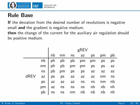
Rule BaseIf the deviation from the desired number of revolutions is negativesmall and the gradient is negative medium,then the change of the current for the auxiliary air regulation shouldbe positive medium.
gREVnb nm ns az ps pm pb
nb ph pb pb pm pm ps psnm ph pb pm pm ps ps azns pb pm ps ps az az az
dREV az ps ps az az az nm nsps az az az ns ns nm nbpm az ns ns ns nb nb nhpb ns ns nm nb nb nb nh
R. Kruse, A. Dockhorn FS – Fuzzy Control Part 3 23 / 59
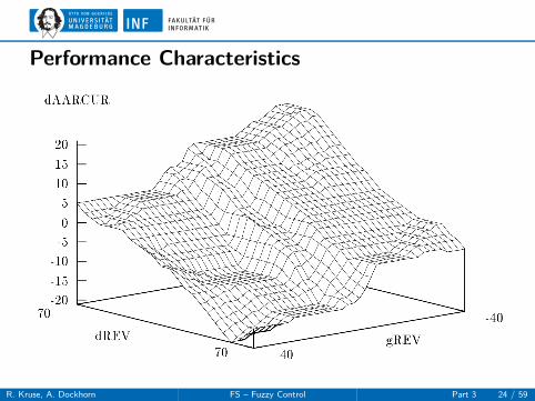
Performance Characteristics
R. Kruse, A. Dockhorn FS – Fuzzy Control Part 3 24 / 59
Example: Automatic Gear Box I
VW gear box with 2 modes (eco, sport) in series line until 1994.
Research issue since 1991: individual adaption of set points and noadditional sensors.
Idea: car “watches” driver and classifies him/her into calm, normal,sportive (assign sport factor [0, 1]), or nervous (calm down driver).
Test car: different drivers, classification by expert (passenger).
Simultaneous measurement of 14 attributes, e.g. , speed, position ofaccelerator pedal, speed of accelerator pedal, kick down, steeringwheel angle.
R. Kruse, A. Dockhorn FS – Fuzzy Control Part 3 25 / 59

Example: Automatic Gear Box IIContinuously Adapting Gear Shift Schedule in VW New Beetle
R. Kruse, A. Dockhorn FS – Fuzzy Control Part 3 26 / 59
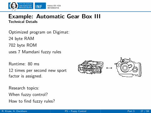
Example: Automatic Gear Box IIITechnical Details
Optimized program on Digimat:
24 byte RAM
702 byte ROM
uses 7 Mamdani fuzzy rules
Runtime: 80 ms
12 times per second new sportfactor is assigned.
Research topics:
When fuzzy control?
How to find fuzzy rules?
R. Kruse, A. Dockhorn FS – Fuzzy Control Part 3 27 / 59

Takagi Sugeno Control

Takagi-Sugeno Controller
Proposed by Tomohiro Takagi and Michio Sugeno.
Modification/extension of Mamdani controller.
Both in common: fuzzy partitions of input domain X1, . . . , Xn.
Difference to Mamdani controller:
• no fuzzy partition of output domain Y ,
• controller rules R1, . . . , Rk are given by
Rr : if ξ1 is A(1)i1,r
and . . . and ξn is A(n)in,r
then ηr = fr (ξ1, . . . , ξn),
fr : X1 × . . . × Xn → Y .
• Generally, fr is linear, i.e. fr (x1, . . . , xn) = a(r)0 +
∑ni=1 a
(r)i xi .
R. Kruse, A. Dockhorn FS – Fuzzy Control Part 3 28 / 59

Takagi-Sugeno Controller: Conclusion
For given input (x1, . . . , xn) and for each Rr , decision logic computestruth value αr of each premise, and then fr (x1, . . . , xn).
Analogously to Mamdani controller:
αr = min{
µ(1)i1,r
(x1), . . . , µ(n)in,r
(xn)}
.
Output equals crisp control value
η =
∑kr=1 αr · fr (x1, . . . , xn)
∑kr=1 αr
.
Thus no defuzzification method necessary.
R. Kruse, A. Dockhorn FS – Fuzzy Control Part 3 29 / 59
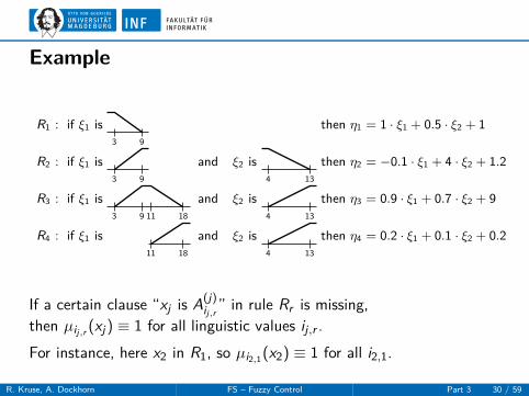
Example
R1 : if ξ1 is
3 9
then η1 = 1 · ξ1 + 0.5 · ξ2 + 1
R2 : if ξ1 is
3 9
and ξ2 is
4 13
then η2 = −0.1 · ξ1 + 4 · ξ2 + 1.2
R3 : if ξ1 is
3 9 11 18
and ξ2 is
4 13
then η3 = 0.9 · ξ1 + 0.7 · ξ2 + 9
R4 : if ξ1 is
11 18
and ξ2 is
4 13
then η4 = 0.2 · ξ1 + 0.1 · ξ2 + 0.2
If a certain clause “xj is A(j)ij,r
” in rule Rr is missing,
then µij,r (xj) ≡ 1 for all linguistic values ij,r .
For instance, here x2 in R1, so µi2,1(x2) ≡ 1 for all i2,1.
R. Kruse, A. Dockhorn FS – Fuzzy Control Part 3 30 / 59

Example: Output Computation
input: (ξ1, ξ2) = (6, 7)
α1 = 1/2 ∧ 1 = 1/2 η1 = 6 + 7/2 + 1 = 10.5
α2 = 1/2 ∧ 2/3 = 1/2 η2 = −0.6 + 28 + 1.2 = 28.6
α3 = 1/2 ∧ 1/3 = 1/3 η3 = 0.9 · 6 + 0.7 · 7 + 9 = 19.3
α4 = 0 ∧ 1/3 = 0 η4 = 6 + 7/2 + 1 = 10.5
output: η = f (6, 7) =1/2 · 10.5 + 1/2 · 28.6 + 1/3 · 19.3
1/2 + 1/2 + 1/3= 19.5
R. Kruse, A. Dockhorn FS – Fuzzy Control Part 3 31 / 59

Example: Passing a Bend
ξ3
ξ1
ξ2ξ4
b
Pass a bend with a car at constant speed.
Measured inputs:
ξ1 : distance of car to beginning of bend
ξ2 : distance of car to inner barrier
ξ3 : direction (angle) of car
ξ4 : distance of car to outer barrier
η = rotation speed of steering wheel
X1 = [0 cm, 150 cm], X2 = [0 cm, 150 cm]
X3 = [−90 ◦, 90 ◦], X4 = [0 cm, 150 cm]
R. Kruse, A. Dockhorn FS – Fuzzy Control Part 3 32 / 59
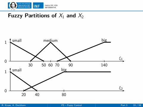
Fuzzy Partitions of X1 and X2
0
1
ξ1
50
small
30 60 90
medium
70 140
big
0
1
ξ2
40
small
20 80
big
R. Kruse, A. Dockhorn FS – Fuzzy Control Part 3 33 / 59
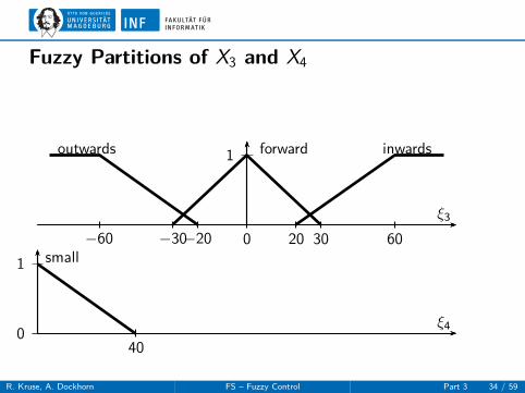
Fuzzy Partitions of X3 and X4
1
ξ3
−20−60
outwards
−30 0 30
forward
20 60
inwards
0
1
ξ4
40
small
R. Kruse, A. Dockhorn FS – Fuzzy Control Part 3 34 / 59

Form of Rules of Car
Rr : if ξ1 is A and ξ2 is B and ξ3 is C and ξ4 is D
then η = p(A,B,C ,D)0 + p
(A,B,C ,D)1 · ξ1 + p
(A,B,C ,D)2 · ξ2
+ p(A,B,C ,D)3 · ξ3 + p
(A,B,C ,D)4 · ξ4
A ∈ {small , medium, big}
B ∈ {small , big}
C ∈ {outwards , forward , inwards}
D ∈ {small}
p(A,B,C ,D)0 , . . . , p
(A,B,C ,D)4 ∈ IR
R. Kruse, A. Dockhorn FS – Fuzzy Control Part 3 35 / 59
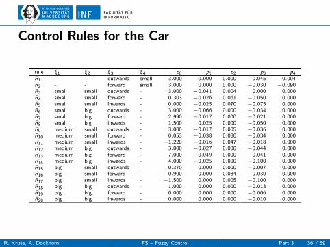
Control Rules for the Car
rule ξ1 ξ2 ξ3 ξ4 p0 p1 p2 p3 p4R1 - - outwards small 3.000 0.000 0.000 −0.045 −0.004R2 - - forward small 3.000 0.000 0.000 −0.030 −0.090R3 small small outwards - 3.000 −0.041 0.004 0.000 0.000R4 small small forward - 0.303 −0.026 0.061 −0.050 0.000R5 small small inwards - 0.000 −0.025 0.070 −0.075 0.000R6 small big outwards - 3.000 −0.066 0.000 −0.034 0.000R7 small big forward - 2.990 −0.017 0.000 −0.021 0.000R8 small big inwards - 1.500 0.025 0.000 −0.050 0.000R9 medium small outwards - 3.000 −0.017 0.005 −0.036 0.000R10 medium small forward - 0.053 −0.038 0.080 −0.034 0.000R11 medium small inwards - −1.220 −0.016 0.047 −0.018 0.000R12 medium big outwards - 3.000 −0.027 0.000 −0.044 0.000R13 medium big forward - 7.000 −0.049 0.000 −0.041 0.000R14 medium big inwards - 4.000 −0.025 0.000 −0.100 0.000R15 big small outwards - 0.370 0.000 0.000 −0.007 0.000R16 big small forward - −0.900 0.000 0.034 −0.030 0.000R17 big small inwards - −1.500 0.000 0.005 −0.100 0.000R18 big big outwards - 1.000 0.000 0.000 −0.013 0.000R19 big big forward - 0.000 0.000 0.000 −0.006 0.000R20 big big inwards - 0.000 0.000 0.000 −0.010 0.000
R. Kruse, A. Dockhorn FS – Fuzzy Control Part 3 36 / 59

Sample Calculation
Assume that the car is 10 cm away from beginning of bend (ξ1 = 10).
The distance of the car to the inner barrier be 30 cm (ξ2 = 30).
The distance of the car to the outer barrier be 50 cm (ξ4 = 50).
The direction of the car be “forward” (ξ3 = 0).
Then according to all rules R1, . . . , R20,only premises of R4 and R7 have a value 6= 0.
R. Kruse, A. Dockhorn FS – Fuzzy Control Part 3 37 / 59

Membership Degrees to Control Car
small medium big
ξ1 = 10 0.8 0 0
small big
ξ2 = 30 0.25 0.167
outwards forward inwards
ξ3 = 0 0 1 0
small
ξ4 = 50 0
R. Kruse, A. Dockhorn FS – Fuzzy Control Part 3 38 / 59

Sample Calculation (cont.)
For the premise of R4 and R7, α4 = 1/4 and α7 = 1/6, resp.
The rules weights α4 = 1/41/4+1/6 = 3/5 for R4 and α5 = 2/5 for R7.
R4 yields
η4 = 0.303 − 0.026 · 10 + 0.061 · 30 − 0.050 · 0 + 0.000 · 50
= 1.873.
R7 yields
η7 = 2.990 − 0.017 · 10 + 0.000 · 30 − 0.021 · 0 + 0.000 · 50
= 2.820.
The final value for control variable is thus
η = 3/5 · 1.873 + 2/5 · 2.820 = 2.2518.
R. Kruse, A. Dockhorn FS – Fuzzy Control Part 3 39 / 59
Fuzzy Control as Similarity-Based
reasoning

Interpolation in the Presence of Fuzziness
Both Takagi-Sugeno and Mamdani are based on heuristics.
They are used without a concrete interpretation.
Fuzzy control is interpreted as a method to specify a non-lineartransition function by knowledge-based interpolation.
A fuzzy controller can be interpreted as fuzzy interpolation.
Now recall the concept of fuzzy equivalence relations (also calledsimilarity relations).
R. Kruse, A. Dockhorn FS – Fuzzy Control Part 3 40 / 59
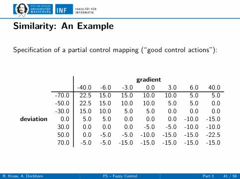
Similarity: An Example
Specification of a partial control mapping (“good control actions”):
gradient-40.0 -6.0 -3.0 0.0 3.0 6.0 40.0
-70.0 22.5 15.0 15.0 10.0 10.0 5.0 5.0-50.0 22.5 15.0 10.0 10.0 5.0 5.0 0.0-30.0 15.0 10.0 5.0 5.0 0.0 0.0 0.0
deviation 0.0 5.0 5.0 0.0 0.0 0.0 -10.0 -15.030.0 0.0 0.0 0.0 -5.0 -5.0 -10.0 -10.050.0 0.0 -5.0 -5.0 -10.0 -15.0 -15.0 -22.570.0 -5.0 -5.0 -15.0 -15.0 -15.0 -15.0 -15.0
R. Kruse, A. Dockhorn FS – Fuzzy Control Part 3 41 / 59

Interpolation of Control Table
There might be additional knowledge available:
Some values are “indistinguishable”, “similar” or “approximatelyequal”.
Or they should be treated in a similar way.
Two problems:
a) How to model information about similarity?
b) How to interpolate in case of an existing similarity information?
R. Kruse, A. Dockhorn FS – Fuzzy Control Part 3 42 / 59

How to Model Similarity?Proposal 1: Equivalence Relation
Definition
Let A be a set and ≈ be a binary relation on A. ≈ is called anequivalence relation if and only if ∀a, b, c ∈ A,(i) a ≈ a (reflexivity)(ii) a ≈ b ↔ b ≈ a (symmetry)(iii) a ≈ b ∧ b ≈ c → a ≈ c (transitivity).
Let us try a ≈ b ⇔ |a − b| < ε where ε is fixed.
≈ is not transitive, ≈ is no equivalence relation.
Recall the Poincaré paradox: a ≈ b, b ≈ c , a 6≈ c .
This is counterintuitive.
R. Kruse, A. Dockhorn FS – Fuzzy Control Part 3 43 / 59

How to Model Similarity?Proposal 2: Fuzzy Equivalence Relation
Definition
A function E : X 2 → [0, 1] is called a fuzzy equivalence relation withrespect to the t-norm ⊤ if it satisfies the following conditions
∀x , y , z ∈ X(i) E (x , x) = 1 (reflexivity)(ii) E (x , y) = E (y , x) (symmetry)(iii) ⊤(E (x , y), E (y , z)) ≤ E (x , z) (t-transitivity).
E (x , y) is the degree to which x ≈ y holds.
E is also called similarity relation, t-equivalence relation,indistinguishability operator, or tolerance relation.
Note that property (iii) corresponds to the vague statement if(x ≈ y) ∧ (y ≈ z) then x ≈ z .
R. Kruse, A. Dockhorn FS – Fuzzy Control Part 3 44 / 59

Fuzzy Equivalence Relations: An Example
Let δ be a pseudo metric on X .
Furthermore ⊤(a, b) = max{a + b − 1, 0} Łukasiewicz t-norm.
Then Eδ(x , y) = 1 − min{δ(x , y), 1} is a fuzzy equivalence relation.
δ(x , y) = 1 − Eδ(x , y) is the induced pseudo metric.
Here, fuzzy equivalence and distance are dual notions in this case.
DefinitionA function E : X 2 → [0, 1] is called a fuzzy equivalence relation if∀x , y , z ∈ X(i) E (x , x) = 1 (reflexivity)(ii) E (x , y) = E (y , x) (symmetry)(iii) max{E (x , y) + E (y , z) − 1, 0} ≤ E (x , z) (Łukasiewicz transitivity).
R. Kruse, A. Dockhorn FS – Fuzzy Control Part 3 45 / 59

Fuzzy Sets as Derived Conceptδ(x , y) = |x − y | metricEδ(x , y) = 1 − min{|x − y |, 1} fuzzy equivalence relation
0
1 µx0
x0 − 1 x x0 x0 + 1
µx0 : X → [0, 1]
x 7→ Eδ(x , x0) fuzzy singleton
µx0 describes “local” similarities.
R. Kruse, A. Dockhorn FS – Fuzzy Control Part 3 46 / 59

Extensional Hull
E : IR × IR → [0, 1], (x , y) 7→ 1 − min{|x − y |, 1} is fuzzyequivalence relation w.r.t. ⊤Łuka.
DefinitionLet E be a fuzzy equivalence relation on X w.r.t. ⊤.µ ∈ F(X ) is extensional if and only if∀x , y ∈ X : ⊤(µ(x), E (x , y)) ≤ µ(y).
DefinitionLet E be a fuzzy equivalence relation on a set X .Then the extensional hull of a set M ⊆ X is the fuzzy set
µM : X → [0, 1], x 7→ sup{E (x , y) | y ∈ M}.
The extensional hull of {x0} is called a singleton.
R. Kruse, A. Dockhorn FS – Fuzzy Control Part 3 47 / 59

Specification of Fuzzy Equivalence Relation
Given a family of fuzzy sets that describes “local” similarities.
0
1
X0
µ1 µ2 µ3 µ4 µ5 µ6 µ7 µ8 µ9
There exists a fuzzy equivalence relation on X with induced singletonsµi if and only if
∀i , j : supx∈X
{µi (x) + µj(x) − 1} ≤ infy∈X
{1 − |µi(y) − µj(y)|}.
If µi(x) + µj(x) ≤ 1 for i 6= j , then there is a fuzzy equivalencerelation E on X
E (x , y) = infi∈I
{1 − |µi(x) − µi(y)|}.
R. Kruse, A. Dockhorn FS – Fuzzy Control Part 3 48 / 59
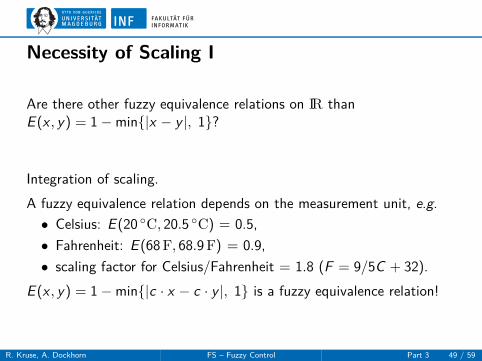
Necessity of Scaling I
Are there other fuzzy equivalence relations on IR thanE (x , y) = 1 − min{|x − y |, 1}?
Integration of scaling.
A fuzzy equivalence relation depends on the measurement unit, e.g.
• Celsius: E (20 ◦C, 20.5 ◦C) = 0.5,
• Fahrenheit: E (68 F, 68.9 F) = 0.9,
• scaling factor for Celsius/Fahrenheit = 1.8 (F = 9/5C + 32).
E (x , y) = 1 − min{|c · x − c · y |, 1} is a fuzzy equivalence relation!
R. Kruse, A. Dockhorn FS – Fuzzy Control Part 3 49 / 59

Necessity of Scaling II
How to generalize scaling concept?
X = [a, b].
Scaling c : X → [0, ∞).
Transformation
f : X → [0, ∞), x 7→
∫ x
ac(t)dt.
Fuzzy equivalence relation
E : X × X → [0, 1], (x , y) 7→ 1 − min{|f (x) − f (y)|, 1}.
R. Kruse, A. Dockhorn FS – Fuzzy Control Part 3 50 / 59

Fuzzy Equivalence Relations: Fuzzy Control
The imprecision of measurements is modeled by a fuzzy equivalencerelations E1, . . . , En and F on X1, . . . , Xn and Y , resp.
The information provided by control expert are
• k input-output tuples (x(r)1 , . . . , x
(r)n , y (r)) and
• the description of the fuzzy equivalence relations for input andoutput spaces, resp.
The goal is to derive a control function ϕ : X1 × . . . × Xn → Y fromthis information.
R. Kruse, A. Dockhorn FS – Fuzzy Control Part 3 51 / 59

Determine Fuzzy-valued Control Functions I
The extensional hull of graph of ϕ must be determined.
Then the equivalence relation on X1 × . . . × Xn × Y is
E ((x1, . . . , xn, y), (x ′1, . . . , x ′
n, y ′))
= min{E1(x1, x ′1), . . . , En(xn, x ′
n), F (y , y ′)}.
R. Kruse, A. Dockhorn FS – Fuzzy Control Part 3 52 / 59
Determine Fuzzy-valued Control Functions II
For Xi and Y , define the sets
X(0)i =
{
x ∈ Xi | ∃r ∈ {1, . . . , k} : x = x(r)i
}
andY (0) =
{
y ∈ Y | ∃r ∈ {1, . . . , k} : y = y (r)}
.
X(0)i and Y (0) contain all values of the r input-output tuples
(x(r)1 , . . . , x
(r)n , y (r)).
For each x0 ∈ X(0)i , singleton µx0 is obtained by
µx0(x) = Ei (x , x0).
R. Kruse, A. Dockhorn FS – Fuzzy Control Part 3 53 / 59
Determine Fuzzy-valued Control Functions III
If ϕ is only partly given, then use E1, . . . , En, F to fill the gaps of ϕ0.
The extensional hull of ϕ0 is a fuzzy set
µϕ0(x′1, . . . , x ′
n, y ′)
= maxr∈{1,...,k}
{
min{E1(x(r)1 , x ′
1), . . . , En(x (r)n , x ′
n), F (y (r), y ′)}}
.
µϕ0 is the smallest fuzzy set containing the graph of ϕ0.
Obviously, µϕ0 ≤ µϕ
µ(x1,...,xn)ϕ0
: Y → [0, 1],
y 7→ µϕ0(x1, . . . , xn, y).
R. Kruse, A. Dockhorn FS – Fuzzy Control Part 3 54 / 59

Reinterpretation of Mamdani Controller
For input (x1, . . . , xn), the projection of the extensional hull of graphof ϕ0 leads to a fuzzy set as output.
This is identical to the Mamdani controller output.
It identifies the input-output tuples of ϕ0 by linguistic rules:
Rr : if X1 is approximately x(r)1
and. . .
and Xn is approximately x (r)n
then Y is y (r).
A fuzzy controller based on equivalence relations behaves like aMamdani controller.
R. Kruse, A. Dockhorn FS – Fuzzy Control Part 3 55 / 59

Reinterpretation of Mamdani Controller
3 fuzzy rules (specified by 3 input-output tuples).
The extensional hull is the maximum of all fuzzy rules.
R. Kruse, A. Dockhorn FS – Fuzzy Control Part 3 56 / 59

References I
R. Kruse, A. Dockhorn FS – Fuzzy Control Part 3 57 / 59

References II
Jantzen, J. (2013).Foundations of fuzzy control: a practical approach.John Wiley & Sons.
Klawonn, F., Gebhardt, J., and Kruse, R. (1995).Fuzzy control on the basis of equality relations with an example from idle speedcontrol.IEEE Transactions on Fuzzy Systems, 3(3):336–350.
Kruse, R., Borgelt, C., Braune, C., Mostaghim, S., and Steinbrecher, M. (2016).Computational intelligence: a methodological introduction.Springer.
Mamdani, E. H. and Assilian, S. (1975).An experiment in linguistic synthesis with a fuzzy logic controller.International journal of man-machine studies, 7(1):1–13.
Michels, K., Klawonn, F., Kruse, R., and Nürnberger, A. (2006).Fuzzy Control: Fundamentals, Stability and Design of Fuzzy Controllers, volume 200of Studies in Fuzziness and Soft Computing.Springer, Berlin / Heidelberg, Germany.
R. Kruse, A. Dockhorn FS – Fuzzy Control Part 3 58 / 59
References III
Sugeno, M. (1985).An introductory survey of fuzzy control.Information sciences, 36(1-2):59–83.
R. Kruse, A. Dockhorn FS – Fuzzy Control Part 3 59 / 59