fuzzy parameters estimation via hybrid...

Fuzzy Parameters Estimation via Hybrid Methods

Sedigheh Danesh ∗†

Abstract

Fuzzy regression analysis is one of the most widely used statistical tech-niques which represents the relation between variables. In this paper,the crisp inputs and the symmetrical triangular fuzzy output are consid-ered. Two hybrid algorithms are considered to fit the fuzzy regressionmodel. In this study, algorithms are based on adaptive neuro-fuzzyinference system. The results are derived based on the V -fold crossvalidation, so that the validity and quality of the suggested methodscan be guaranteed. Finally, using the numerical examples, the perfor-mance of the suggested methods are compared with the other ones,such as linear programming (LP) and quadratic programming (QP).Based on examples, hybrid methods are verified for the prediction.

Keywords: linear programming, quadratic programming, adaptive neuro-fuzzyinference system.

2000 AMS Classification: 92B20, 03B52

1. Introduction

The concept of fuzzy regression analysis was introduced by Tanaka et al. [39]in 1982. Tanaka et al. [38] regarded fuzzy data as a possibility distribution. So,they supposed the deviations between the observed values and the estimated val-ues are due to the fuzziness of the system structure. In general, several fuzzyregression techniques have been proposed based on fuzzy least squares (FLS) andmathematical programming methods, such as linear programming (LP) or qua-dratic programming (QP) that minimize the total spread of the output. FLS andmathematical programming methods were initially proposed by Diamond [11] andTanaka et al. (see, e.g. [36, 37, 38]) respectively. Moreover, the several variantsFLS (see, e.g. [1, 5, 24, 29]) and mathematical programming (see, e.g. [27, 28])have been applied for the fuzzy linear regression problem. In the fuzzy literatures,the several extensions of these methods have been proposed in a non-parametriccontext. For fuzzy nonparametric regression, Cheng and Lee [6] proposed k-NNand kernel smoothing techniques, Farnoosh et al. [14] introduced a modificationon ridge estimation and Wang et al. [40] proposed local linear smoothing tech-nique. Razzaghnia and Danesh [30] analyzed local linear smoothing technique innonparametric regression with trapezoidal fuzzy data. In the recent years, theartificial intelligent modeling techniques have been utilized to approximate thenon-linear problems, the complex behaviors and the prediction of the regression

∗Department of Mathematics, East Tehran Branch, Islamic Azad university, Tehran, Iran,

Email: [email protected], [email protected].†Corresponding Author.

2

parameters. Ishibuchi et al. (see, e.g. [16, 17, 18]) have introduced fuzzy regres-sion analysis by using neural networks and proposed a learning algorithm of thefuzzy neural networks with the triangular fuzzy weights. Mosleh et al. [25, 26]used a novel hybrid method based on fuzzy neural network for fuzzy coefficientsprediction of fuzzy linear and nonlinear regression models and for solving a systemof fuzzy differential equations. Shapiro [32] proposed the merge of neural networks,fuzzy logic, and genetic algorithms. Kraily et al. [23] have utilized k-NN graphof high dimensional data as efficient representation of the hidden structure of theclustering problem. Cluster centers are fine-tuned by minimizing fuzzy-weightedgeodesic distances. Their algorithm is capable to cluster networks. In 1993, Jang[20] proposed adaptive network based on inference systems (ANFIS) that com-bines the artificial neural networks and the fuzzy systems. It has the benefits ofthe two models. In 1998, Cheng and Lee [2, 4] formulated the ANFIS model andradial basis function networks for the fuzzy regression and Dalkilic and Apaydin[7, 8] used the ANFIS model to analyze the switching regression and estimate thefuzzy regression parameters in 2009 and 2014. Also, Danesh et al. [9] proposedthe fuzzy least squares problem based on Diamond’s distance to optimize the con-sequent parameters in the hybrid algorithm of the adaptive neuro-fuzzy inferencesystem method. Kayacan and Khanesar [21] have been proposed a novel hybridtraining method that uses particle swarm optimization (PSO) for the training ofthe antecedent parts of type 2 fuzzy neural networks (T2FNNs) and SMC-basedtraining methods for the training of parameters of their consequent parts. Gaxiolaet al. [15] presented the optimization of type-2 fuzzy inference systems using ge-netic algorithms (GAs) and PSO. So in recently years, ANFIS has been applied indifferent areas such as medicine, industry, geography, and econometrics. In medicalfield, Sridevi and Nirmala [33] utilized ANFIS to perceive and show clinical resultsof prenatal Truncus Arteriosus congenital heart defect, and in geography, Dewanet al. [10] proposed that ANFIS model could be utilized for prediction of ultimatetensile strength of Friction-stir-welding joints. They considered three critical pro-cess parameters including spindle speed, plunge force and welding speed. Fangand Lee [13] have used a self-tuning controller based on a neuro-fuzzy algorithmto control the rotation speed of the outboard thrusters for the optimal adjustmentof the ship position, heading and for path tracking. In industry, Sarhadi et al.[31] have proposed a novel adaptive predictive control method based on adaptiveneuro-fuzzy inference system for a class of nonlinear industrial processes. Linearpart is approximated using least squares estimation technique, and the nonlin-ear part is identified using an ANFIS-based identifier. In econometrics, Cheng etal. [3] presented that artificial intelligence approaches are applicable to cost esti-mating problems related to expert systems, case based reasoning (CBR), neuralnetwork (NN), fuzzy logic (FL), genetic algorithms (GA) and derivatives. In thisstudy, the linear programming method is proposed to optimize the consequentparameters in the hybrid algorithm of the adaptive neuro-fuzzy inference systemmethod. Also, hybrid algorithms based on linear programming and fuzzy leastsquare are designed to predict fuzzy regression model and reduce error. In thesealgorithms, the gradient descent method is used to compute the premise parame-ters (fuzzy weights). Also, the linear programming method (FWLP) and the fuzzy

3

least squares (FWLS) to optimize the consequent parameters. Hybrid methods arecompared with LP and QP methods. It is demonstrated that hybrid methods havelower error than LP and QP in the prediction.

This paper includes four sections. In section 2, the concepts and formulationsof the different models are explained. In section 3, ANFIS method is extended infuzzy regression and the consequent parameters are obtained by using the linearprogramming and fuzzy least squares based on Diamond’s distance. Two examplesare used to illustrate the methods in section 4, and the analysis of the results isdiscussed in section 5.

2. Material and Methods

Definition 1 : Suppose that X = (lX , aX , rX) is a triangular fuzzy number sothat aX , lX and rX and are the center, the lower and the upper limits beingthis fuzzy number, respectively. The membership function of X = (lX , aX , rX) isdefined as follows:

µx(z) =

L( aX−z

aX−lX), lX < z < aX ,

R( z−aX

rX−aX), aX < z < rX ,

0, otherwise.

.(2.1)

Let A = (lA, aA, rA) and B = (lB , aB , rB), lA, rA, lB , rB ≥ 0 be any twotriangular fuzzy numbers. So, the distance between A and B can be expressed as[11]:

d2(A,B) = (lB − lA)2

+ (aB − aA)2

+ (rB − rA)2.(2.2)

This distance measures the closeness between the membership functions of twotriangular fuzzy numbers. The membership functions A and B are equal whend2(A,B) = 0. Also, the result of addition of triangular fuzzy numbers is a trian-gular fuzzy number again.

Definition 2 : The function f(x) is a mapping from x to Y where xj =(xj0, xj1, . . . , xjp)(j = 1, . . . , n) is a p-dimentional vector crisp independent vari-able and domain is assumed to be D⊂Rp. Consider the following the fuzzy regres-sion model:

Y = f(x) {+} ε = (l(x), a(x), r(x))LR {+} ε,(2.3)

where Y has the fuzzy structure and ε represents the regression error with con-ditional mean zero and variance σ2(x) given x. Y is the response variable. Asymmetric triangular fuzzy number Yj can be written as Yj = (aj , βj) where ajand βj are the center and the spread of a symmetric triangular fuzzy numberrespectively, and βj = rj − aj = aj − lj .

2.1. Forecasting methods. In this section, we will briefly describe LP and QPmethods.

2.1.1. Fuzzy regression with linear programming (LP). In this study, we considera fuzzy regression model with crisp inputs and triangular fuzzy output. Considerthe following fuzzy regression model as:

Yj = p0 + p1xj1 + p2xj2 + . . .+ ppxjp = Pxj , j = 1, . . . , n,(2.4)

4

where n is the number of data points, xj = (xj0, xj1, . . . , xjp) is a p-dimensional in-put vector of the independent variables at the jth observation, P = (p0, p1, . . . , pp)is a vector of unknown fuzzy parameters and Yj is the jth observed value ofthe dependent variables. P can be denoted in vector form as P = {a, b} whereb = (b0, b1, . . . , bp), α = (α0, α1, . . . , αp), bi is the center value and αi is the spreadvalue of pi, i = 0, . . . , p. Also, Yj = (aj , βj) is symmetric triangular fuzzy numberwhere aj and βj are the center and the spread, respectively. Also according to theproposed method by Tanaka et al. [38], the fuzzy regression parameters can beobtained by solving the following linear programming (LP) model:

min L =

n∑j=1

p∑i=0

αi|xji|,(2.5)

so that, the following two constraints must be established:

p∑i=0

bi|xji| − (1− h)

p∑i=0

αi|xji| ≤ aj − (1− h)βj ,(2.6)

p∑i=0

bi|xji|+ (1− h)

p∑i=0

αi|xji| ≥ aj + (1− h)βj ,(2.7)

and, αi ≥ 0, i = 0, . . . , p, j = 1, . . . , n. In this model, the constrains guaranteethat the support of the estimated values from the regression model includes thesupport of the observed values in h-level (0 < h ≤ 1).

2.1.2. Quadratic programming. Let the observed values Yj = (lyj, ayj

, ryj) and

the predicted values Yj = (lyj , ayj , ryj ) are asymmetric triangular fuzzy numbers(j = 1, . . . , n) where lyj , ayj and ryj are the lower, the center and the upper limits

of the observed fuzzy outputs and lyj , ayj and ryj are the lower, the center, andthe upper limits of the predicted fuzzy outputs. In this method, the proposedobjective function in [12] is applied for the crisp inputs and the asymmetric fuzzyoutput that is defined as follows:

n∑j=0

k1(ayj− ayj

)2 + (k2(lyj− lyj

)2 + (ryj− ryj

)2).(2.8)

Where k1 > k2 allow to give more importance to the central tendency and k1 < k2to reduce of estimates uncertainty in the process. Suppose Yj = (ayj , βyj ) and

Yj = (ayj , βyj) are two symmetric fuzzy numbers, where ayj

and βyjare the center

and the spread of the observed fuzzy outputs, ayjand βyj

are the center and spread

of the predicted fuzzy outputs, lyj= ayj

− βyj, ryj

= ayj+ βyj

, lyj= ayj

− βyj

and ryj= ayj

+ βyj. In this study, k1 = k2 is considered. By substituting lyj

, ryj,

lyjand ryj

in Eq. (2.8), it can be rewritten as follows:

n∑j=0

((ayj − βyj )− (ayj − βyj ))2 + (ayj − ayj )2 + ((ayj + βyj )− (ayj + βyj ))2

5

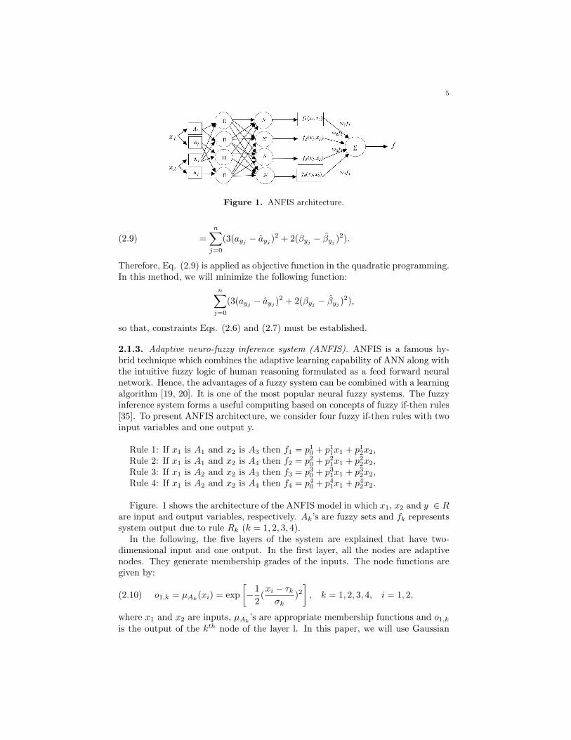
Figure 1. ANFIS architecture.

=

n∑j=0

(3(ayj− ayj

)2 + 2(βyj− βyj

)2).(2.9)

Therefore, Eq. (2.9) is applied as objective function in the quadratic programming.In this method, we will minimize the following function:

n∑j=0

(3(ayj− ayj

)2 + 2(βyj− βyj

)2),

so that, constraints Eqs. (2.6) and (2.7) must be established.

2.1.3. Adaptive neuro-fuzzy inference system (ANFIS). ANFIS is a famous hy-brid technique which combines the adaptive learning capability of ANN along withthe intuitive fuzzy logic of human reasoning formulated as a feed forward neuralnetwork. Hence, the advantages of a fuzzy system can be combined with a learningalgorithm [19, 20]. It is one of the most popular neural fuzzy systems. The fuzzyinference system forms a useful computing based on concepts of fuzzy if-then rules[35]. To present ANFIS architecture, we consider four fuzzy if-then rules with twoinput variables and one output y.

Rule 1: If x1 is A1 and x2 is A3 then f1 = p10 + p11x1 + p12x2,Rule 2: If x1 is A1 and x2 is A4 then f2 = p20 + p21x1 + p22x2,Rule 3: If x1 is A2 and x2 is A3 then f3 = p30 + p31x1 + p32x2,Rule 4: If x1 is A2 and x2 is A4 then f4 = p40 + p41x1 + p42x2.

Figure. 1 shows the architecture of the ANFIS model in which x1, x2 and y ∈ Rare input and output variables, respectively. Ak’s are fuzzy sets and fk representssystem output due to rule Rk (k = 1, 2, 3, 4).

In the following, the five layers of the system are explained that have two-dimensional input and one output. In the first layer, all the nodes are adaptivenodes. They generate membership grades of the inputs. The node functions aregiven by:

o1,k = µAk(xi) = exp

[−1

2(xi − τkσk

)2], k = 1, 2, 3, 4, i = 1, 2,(2.10)

where x1 and x2 are inputs, µAk’s are appropriate membership functions and o1,k

is the output of the kth node of the layer l. In this paper, we will use Gaussian

6

membership function where parameters τk and σk represent the center and thewidth, respectively.

In the second layer, the nodes are also fixed. The outputs of this layer can becalculated as:

o2,k = ωk = µAk(x1).µAk

(x2), k = 1, 2, 3, 4.(2.11)

In Figure. 1, implication has been shown with notation∏

.. In the third layer, thenodes are fixed nodes. It calculates the ratio of a rule’s firing of all the rules. Theoutputs of this layer can be calculated as:

o3,k = ωk =ωk∑4j=0 ωk

, k = 1, 2, 3, 4.(2.12)

This is called normalized firing strength and it has been shown with notation Nin Figure. 1. In the fourth layer, the node is an adaptive node. The node functionassociated in the level 4 is a linear function. The outputs of this layer can berepresented as below:

o4,k = ωkfk = ωk(pk0 + pk1x1 + pk2x2), k = 1, 2, 3, 4.(2.13)

In this work, pki will be assumed to be a triangular fuzzy number for k = 1, . . . , 4and i = 0, 1, 2.

In the fifth layer, the single node carries out the sum of inputs of all the layers.The overall output of the structure is expressed as:

o5,k =

4∑j=0

ωkfk.(2.14)

3. Methodology of the proposed method

In Eq. (2.14), assume that the consequence parameter pki is a symmetric trian-gular fuzzy number and is represented as pk

j = (bki , αki ), i = 0, . . . , p, k = 1, . . . ,m.

Also, Yj and Yj are symmetric triangular fuzzy numbers and are represented by

Yj = (ayj, βyj

) and Yj = (ayj, βyj

), j = 1, . . . , n, where n is the number of datapoints, ayj

is center value and βyjis spread value of Yj , and ayj

is center value

and βyj is spread value of Yj .Suppose xj = (xj0, xj1, . . . , xjp) is a p-dimensional input vector of the inde-

pendent variables at the jth observation, also, P = (p0, p1, . . . , pp) is a vectorof unknown fuzzy parameters and Yj is the jth observed value of the dependentvariables.pi, i = 0, . . . , p, can be denoted in vector form as pi = {a, b} whereb = (bk0 , b

k1 , . . . , b

kp) and α = (αk

0 , αk1 , . . . , α

kp), k = 1, . . . ,m, where bki is center

value and αk is spread value of pi, i = 0, . . . , p. So from the above definitions,using fuzzy arithmetic and substituting pki into Eq. (2.14), it can be expressed as:

Yj =

m∑k=1

p∑i=0

bki ωxji +

m∑k=1

p∑i=0

αki ωxji.(3.1)

So,

ay =

m∑k=1

p∑i=0

bki ωxji,(3.2)

7

and

βyj=

m∑k=1

p∑i=0

αki ωxji.(3.3)

where wk is known. In this paper, the fuzzy weights (premise parameters) areupdated by using the back propagation. In this method, we only use the first partof the Eq. (2.9) to update fuzzy weights that is defined as:

e =

n∑j=1

e2j =

n∑j=1

(aj − aj)2,(3.4)

and the influence of the spread is ignored. So, the back propagation error for eachlayer is obtained as follows [2, 20]:

el,k =

Ml+1∑r=1

el+1∂Al+1,r

∂ol,k,(3.5)

el,k is the back propagation error of the kth node of the layer l. Al+1,r, is the node

function of the rth node of (l + 1)th

layer, ol,k represents the output kth node of

the layer l and Ml+1 is the total number of nodes in the (l + 1)th

layer. So, errorof the final output node is calculated as:

e5,1 =∂e2j∂yj

= −(aj − aj).(3.6)

So, the gradient vector is defined as the error measure derivatives with respectto each parameter. The derivative of the overall error measure e with respect toparameter δ is:

∂e

∂δ=

1

n

n∑j=1

∂e2j∂δ

=

n∑j=1

el,k∂ol,k∂δ

.(3.7)

Thus, the updating formula for δ is defined as:

∆δ = −ϑ∂e∂δ,(3.8)

where ϑ is the learning rate. In this paper, the consequence parameters pki areobtained by solving linear programming (LP) and fuzzy least squares problem.Two hybrid methods will be explained in the following.

3.1. Linear programming in the prediction of the consequence param-eters. In Eq. (3.1), it was shown that

Yj =∑m

k=1

∑pi=0 b

ki ωxji +

∑mk=1

∑pi=0 α

ki ωxji.

The consequence parameters bki and αki can be obtained by solving the following

linear programming (LP) model:

min∑m

k=1

∑pi=0 α

ki ωxji

8

So that, the following two constraints must be established:m∑

k=1

p∑i=0

bki ωxji − (1− h)

m∑k=1

p∑i=0

αki ωxji ≤ aj − (1− h)βj ,(3.9)

m∑k=1

p∑i=0

bki ωxji + (1− h)

m∑k=1

p∑i=0

αki ωxji ≥ aj + (1− h)βj ,(3.10)

and, αiω ≥ 0, i = 0, . . . , p, k = 1, . . . ,m, j = 1, . . . , n.

3.2. Fuzzy least squares problem in the prediction of the consequenceparameters. By using fuzzy least squares problem, we can obtain the conse-quence parameters estimation for the fuzzy regression model as follows:

(bki )T = (XTX)−1XTAY ,(3.11)

(αki )T = (XTX)

−1XTαY ,(3.12)

where,

X =

ω11 ω12 . . . ω1m ω11x11 . . . ω1mx11 . . . ω11x1p . . . ω1mx1pω21 ω22 . . . ω2m ω21x21 . . . ω2mx21 . . . ω21x2p . . . ω2mx2p. . . . . . .. . . . . . .. . . . . . .ωn1 ωn2 . . . ωnm ωn1xn1 . . . ωnmxn1 . . . ωn1xnp . . . ωnmxnp

AY =

ay1

ay2

.

.

.ayn

, αY =

αy1

αy2

.

.

.αyn

, (bki )T =

b10...

bm0...

b1p...

bmp

, (αki )T =

α10

.

.

.αm0

.

.

.α1p

.

.

.αmp

.

3.3. Modelling Performance Criterion. In the following, we putERROR = 1

n

∑nj=1(Yj − Yj)2

=1

n

n∑j=0

(3(ayj−

m∑k=1

p∑i=0

bki ωxji)2 + 2(βyj

−m∑

k=1

p∑i=0

αki ωxji)

2).(3.13)

and use Eq. (3.13) as a quantity to measure bias between the observed values,

Yj = (lj , aj , rj), and the predicted values, Yj = (lj , aj , rj), for all Xjs (j =

1, . . . , n) where lj , aj , rj , lj , aj , and rj are lower, center and upper of the observed

9

fuzzy outputs and, lower, center and upper of the estimated fuzzy outputs. Largevalue of this quantity indicates lack-of-fit and too small value reflects over-fit forthe observed fuzzy outputs. Also, we use the method of Kim and Bishu (1998) [22]for evaluation of the performance of the suggested models. In this method, theabsolute difference between the observed membership values and the estimatedvalues are calculated. This method is defined as:

Ej =

∫S(Yj)

⋃S(Yj)

|Yj − Yj |dy,(3.14)

where S(Yj) and S(Yj) are support of Yj and Yj , respectively. In other words, Ej

is the error in our estimation. If Ej trend to zero, then the fitting is the best. Inthis study, an ’epoch’ (EP) means a complete presentation of the entire set of thetraining data.

3.4. The learning algorithm of FWLP method. For forecasting model pa-rameters, the steps taken can be summarized as follows:

Step 1: Input value h and EP.Step 2: Divide all data into two subsets, train data (TRD) and test data set

(TED) by V-fold cross validation technique. For each of V folds, use V-1 folds fortraining and the remaining one for testing.

Step 3: Determine the initial values of the premise parameters (fuzzy weights)by using Eq. (3.8).

Step 4: Identify the consequent parameters by solving the linear programmingEqs. (3.9) and (3.10).

Step 5: Terminate the training of network when average of ERROR in Eq. (3.4)is smaller than a predefined small number or reach the last number of predefinedepoch, otherwise go to Step 2 and update the premise parameters.

Step 6: Determine the error values of Ej and ERROR in Eqs. (3.13) and (3.14)for the evaluation of the designed method.

Step 7: Repeat steps 3 to 6 for each of the V-folds.

3.5. The learning algorithm of FWLS method. This algorithm is similarto FWLP’s except that the consequent parameters are identified by fuzzy leastsquares problem Eqs. (3.11) and (3.12) in step 4. In this paper, we use MATLABsoftware tool for codding.

4. Numerical examples

In order to demonstrate the applicability of the hybrid algorithms, numericalexamples are used. Also, the obtained results of the different methods are com-pared.

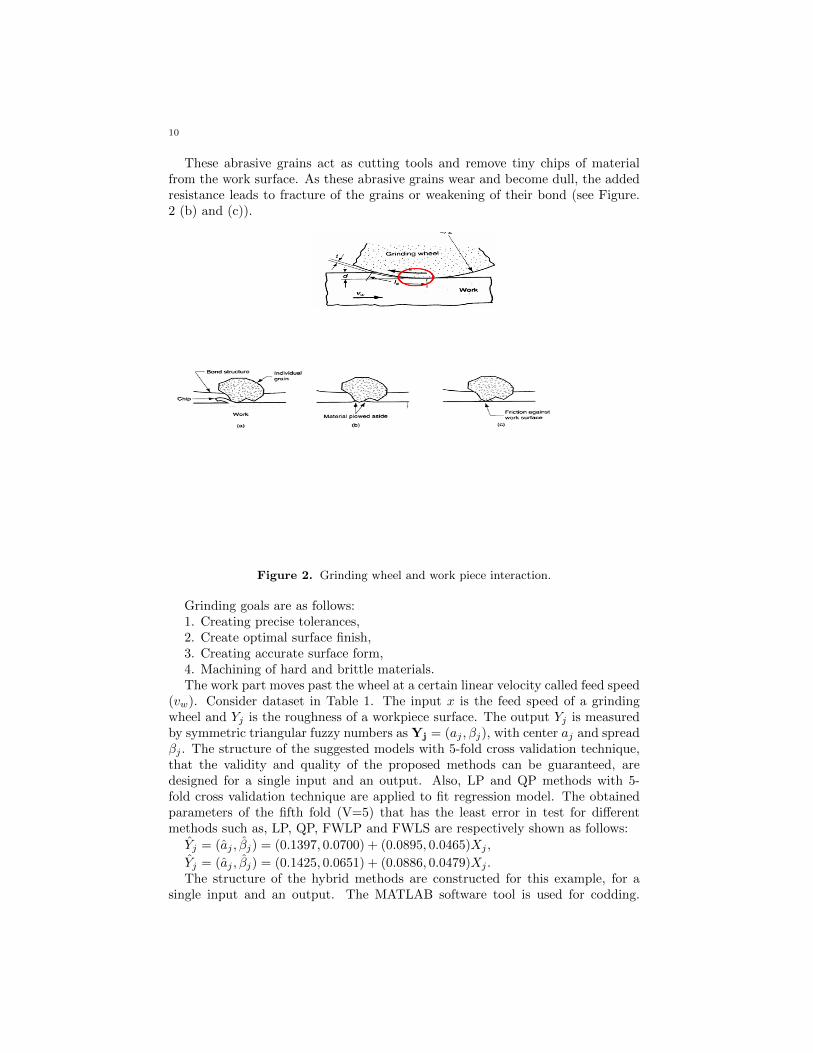
Example 1: Grinding is a material removal and surface generation processused to shape and finish components made of metals and other materials. Theprecision and the finish surface obtained through grinding can be up to ten timesbetter than either turning or milling. As seen in Figure. 2(a), grinding employs anabrasive product and usually a rotating wheel brought into controlled contact witha work surface. The grinding wheel is composed of abrasive grains held togetherin a binder.

10

These abrasive grains act as cutting tools and remove tiny chips of materialfrom the work surface. As these abrasive grains wear and become dull, the addedresistance leads to fracture of the grains or weakening of their bond (see Figure.2 (b) and (c)).

Figure 2. Grinding wheel and work piece interaction.

Grinding goals are as follows:1. Creating precise tolerances,2. Create optimal surface finish,3. Creating accurate surface form,4. Machining of hard and brittle materials.The work part moves past the wheel at a certain linear velocity called feed speed

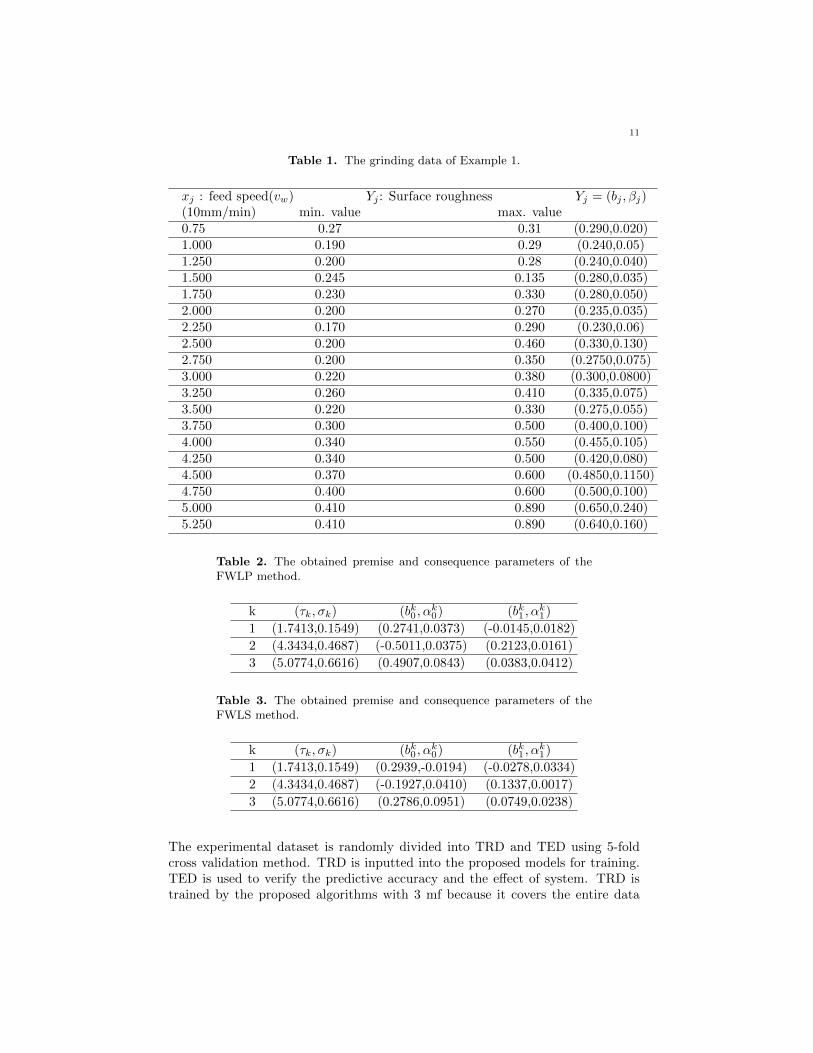
(vw). Consider dataset in Table 1. The input x is the feed speed of a grindingwheel and Yj is the roughness of a workpiece surface. The output Yj is measuredby symmetric triangular fuzzy numbers as Yj = (aj , βj), with center aj and spreadβj . The structure of the suggested models with 5-fold cross validation technique,that the validity and quality of the proposed methods can be guaranteed, aredesigned for a single input and an output. Also, LP and QP methods with 5-fold cross validation technique are applied to fit regression model. The obtainedparameters of the fifth fold (V=5) that has the least error in test for differentmethods such as, LP, QP, FWLP and FWLS are respectively shown as follows:

Yj = (aj , βj) = (0.1397, 0.0700) + (0.0895, 0.0465)Xj ,

Yj = (aj , βj) = (0.1425, 0.0651) + (0.0886, 0.0479)Xj .The structure of the hybrid methods are constructed for this example, for a

single input and an output. The MATLAB software tool is used for codding.

11

Table 1. The grinding data of Example 1.

xj : feed speed(vw) Yj : Surface roughness Yj = (bj , βj)(10mm/min) min. value max. value0.75 0.27 0.31 (0.290,0.020)1.000 0.190 0.29 (0.240,0.05)1.250 0.200 0.28 (0.240,0.040)1.500 0.245 0.135 (0.280,0.035)1.750 0.230 0.330 (0.280,0.050)2.000 0.200 0.270 (0.235,0.035)2.250 0.170 0.290 (0.230,0.06)2.500 0.200 0.460 (0.330,0.130)2.750 0.200 0.350 (0.2750,0.075)3.000 0.220 0.380 (0.300,0.0800)3.250 0.260 0.410 (0.335,0.075)3.500 0.220 0.330 (0.275,0.055)3.750 0.300 0.500 (0.400,0.100)4.000 0.340 0.550 (0.455,0.105)4.250 0.340 0.500 (0.420,0.080)4.500 0.370 0.600 (0.4850,0.1150)4.750 0.400 0.600 (0.500,0.100)5.000 0.410 0.890 (0.650,0.240)5.250 0.410 0.890 (0.640,0.160)

Table 2. The obtained premise and consequence parameters of theFWLP method.

k (τk, σk) (bk0 , αk0) (bk1 , α

k1)

1 (1.7413,0.1549) (0.2741,0.0373) (-0.0145,0.0182)

2 (4.3434,0.4687) (-0.5011,0.0375) (0.2123,0.0161)

3 (5.0774,0.6616) (0.4907,0.0843) (0.0383,0.0412)

Table 3. The obtained premise and consequence parameters of theFWLS method.

k (τk, σk) (bk0 , αk0) (bk1 , α

k1)

1 (1.7413,0.1549) (0.2939,-0.0194) (-0.0278,0.0334)

2 (4.3434,0.4687) (-0.1927,0.0410) (0.1337,0.0017)

3 (5.0774,0.6616) (0.2786,0.0951) (0.0749,0.0238)

The experimental dataset is randomly divided into TRD and TED using 5-foldcross validation method. TRD is inputted into the proposed models for training.TED is used to verify the predictive accuracy and the effect of system. TRD istrained by the proposed algorithms with 3 mf because it covers the entire data

12

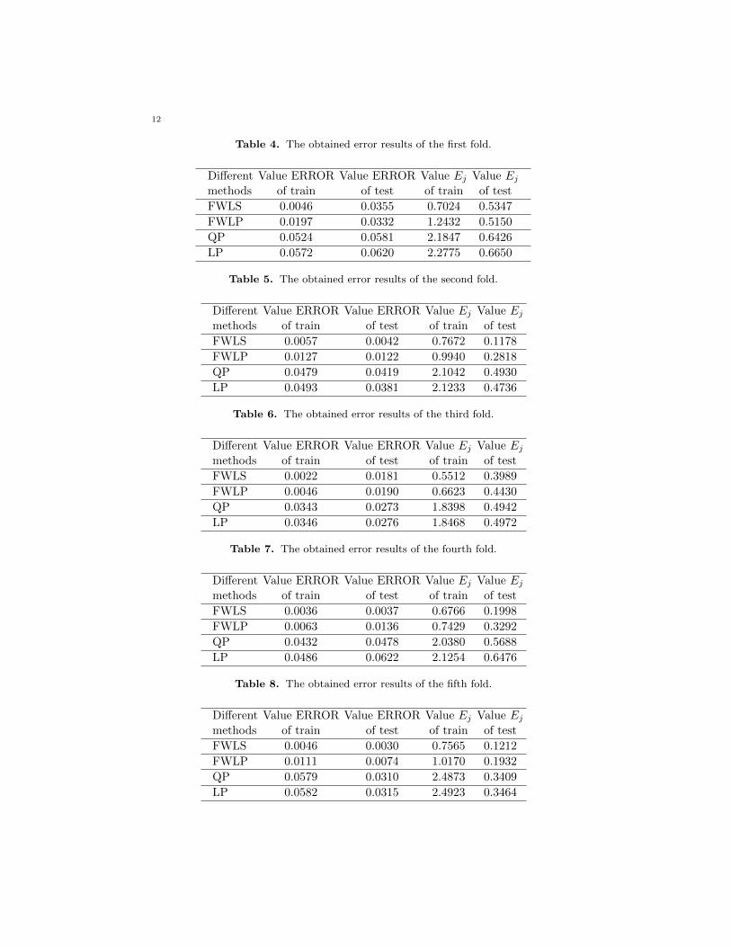
Table 4. The obtained error results of the first fold.

Different Value ERROR Value ERROR Value Ej Value Ej

methods of train of test of train of test

FWLS 0.0046 0.0355 0.7024 0.5347

FWLP 0.0197 0.0332 1.2432 0.5150

QP 0.0524 0.0581 2.1847 0.6426

LP 0.0572 0.0620 2.2775 0.6650

Table 5. The obtained error results of the second fold.



FWLS 0.0057 0.0042 0.7672 0.1178

FWLP 0.0127 0.0122 0.9940 0.2818

QP 0.0479 0.0419 2.1042 0.4930

LP 0.0493 0.0381 2.1233 0.4736

Table 6. The obtained error results of the third fold.



FWLS 0.0022 0.0181 0.5512 0.3989

FWLP 0.0046 0.0190 0.6623 0.4430

QP 0.0343 0.0273 1.8398 0.4942

LP 0.0346 0.0276 1.8468 0.4972

Table 7. The obtained error results of the fourth fold.



FWLS 0.0036 0.0037 0.6766 0.1998

FWLP 0.0063 0.0136 0.7429 0.3292

QP 0.0432 0.0478 2.0380 0.5688

LP 0.0486 0.0622 2.1254 0.6476

Table 8. The obtained error results of the fifth fold.



FWLS 0.0046 0.0030 0.7565 0.1212

FWLP 0.0111 0.0074 1.0170 0.1932

QP 0.0579 0.0310 2.4873 0.3409

LP 0.0582 0.0315 2.4923 0.3464

13

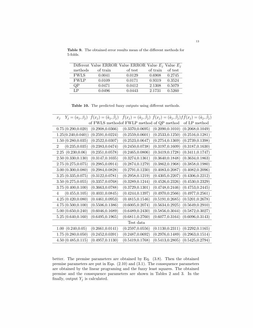
Table 9. The obtained error results mean of the different methods for5-folds.


methods of train of test of train of testFWLS 0.0041 0.0129 0.6908 0.2745FWLP 0.0109 0.0171 0.9319 0.3524QP 0.0471 0.0412 2.1308 0.5079LP 0.0496 0.0443 2.1731 0.5260

Table 10. The predicted fuzzy outputs using different methods.

xj Yj = (aj , βj) f(xj) = (aj , βj) f(xj) = (aj , βj) f(xj) = (aj , βj)ff(xj) = (aj , βj)

of FWLS methodof FWLP method of QP method of LP method

0.75 (0.290,0.020) (0.2908,0.0366) (0.3370,0.0695) (0.2090,0.1010) (0.2068,0.1049)

1.25(0.240,0.040)) (0.2591,0.0224) (0.2559,0.0601) (0.2533,0.1250) (0.2516,0.1281)

1.50 (0.280,0.035) (0.2522,0.0307) (0.2523,0.0647) (0.2754,0.1369) (0.2739,0.1398)

2 (0.235,0.035) (0.2383,0.0474) (0.2450,0.0738) (0.3197,0.1609) (0.3187,0.1630)

2.25 (0.230,0.06) (0.2351,0.0578) (0.2465,0.0806) (0.3419,0.1728) (0.3411,0.1747)

2.50 (0.330,0.130) (0.3147,0.1035) (0.3274,0.1361) (0.3640,0.1848) (0.3634,0.1863)

2.75 (0.275,0.075) (0.2985,0.0914) (0.2874,0.1279) (0.3862,0.1968) (0.3858,0.1980)

3.00 (0.300,0.080) (0.2984,0.0828) (0.2791,0.1230) (0.4083,0.2087) (0.4082,0.2096)

3.25 (0.335,0.075) (0.3122,0.0781) (0.2958,0.1219) (0.4305,0.2207) (0.4306,0.2212)

3.50 (0.275,0.055) (0.3357,0.0768) (0.3289,0.1244) (0.4526,0.2326) (0.4530,0.2329)

3.75 (0.400,0.100) (0.3663,0.0788) (0.3729,0.1301) (0.4748,0.2446) (0.4753,0.2445)

4 (0.455,0.105) (0.4031,0.0845) (0.4244,0.1397) (0.4970,0.2566) (0.4977,0.2561)

4.25 (0.420,0.080) (0.4461,0.0953) (0.4815,0.1546) (0.5191,0.2685) (0.5201,0.2678)

4.75 (0.500,0.100) (0.5506,0.1386) (0.6005,0.2074) (0.5634,0.2925) (0.5649,0.2910)

5.00 (0.650,0.240) (0.6046,0.1689) (0.6489,0.2430) (0.5856,0.3044) (0.5872,0.3027)

5.25 (0.640,0.160) (0.6495,0.1965) (0.6811,0.2760) (0.6077,0.3164) (0.6096,0.3143)

Test data

1.00 (0.240,0.05) (0.2661,0.0141) (0.2597,0.0556) (0.1130,0.2311) (0.2292,0.1165)

1.75 (0.280,0.050) (0.2452,0.0391) (0.2487,0.0692) (0.2976,0.1489) (0.2963,0.1514)

4.50 (0.485,0.115) (0.4957,0.1130) (0.5419,0.1768) (0.5413,0.2805) (0.5425,0.2794)

better. The premise parameters are obtained by Eq. (3.8). Then the obtainedpremise parameters are put in Eqs. (2.10) and (3.1). The consequence parametersare obtained by the linear programing and the fuzzy least squares. The obtainedpremise and the consequence parameters are shown in Tables 2 and 3. In thefinally, output Yj is calculated.

14

For example, f(x18) can be calculated using the FWLP method as follows. Inthe first, w18,k are calculated for k = 1, 2, 3. So using the premise parameters ofTable 2, Eqs. (2.10) and (2.12), and x18 = 5, w18,k are equivalent:

w18,1 = exp

[−1

2(5− 1.7431

0.1549)2]

= 6.8674e− 97, w18,2 = 0.3749, w18,3 = 0.9932,

and,∑3k=1 w18,k = 6.8674e− 97 + 0.3749 + 0.9932 = 1.3681.

Therefore, w18,1 = 6.8674e−971.3681 = 5.0197e − 97, w18,2 = 0.3749

1.3681 = 0.2740, w18,3 =0.99321.3681 = 0.7260.

In the following, w18,k and the obtained consequence parameters (bki , aki , k =

1, 2, 3, i = 0, 1) of Table 2 are substituted in Eqs. (3.11) and (3.12). In the finally,

f(x18) is computed as follows:

a18 = (5.0197e−97)(0.2741)+(0.274)(−0.5011)+(0.726)(0.4907)+(5.0197e−97)

(−0.0145)(5) + (0.2740)(0.2123)(5) + (0.7260)(0.0383)(5) = 0.6488,and,

β18 = (5.0197e−97)(0.0373)+(0.274)(0.0375)+(0.726)(0.0843)+(5.0197e−97)(0.0182)(5) + (0.2740)(0.0161)(5) + (0.7260)(0.0412)(5) = 0.2431.

Thereupon,

f(x18) = (a18, β18) = (0.6488, 0.2431).

Also in the FWLS method, f(x18) is calculated as the FWLP method.The obtained results of the different methods are displayed in Tables 4-9. Also,

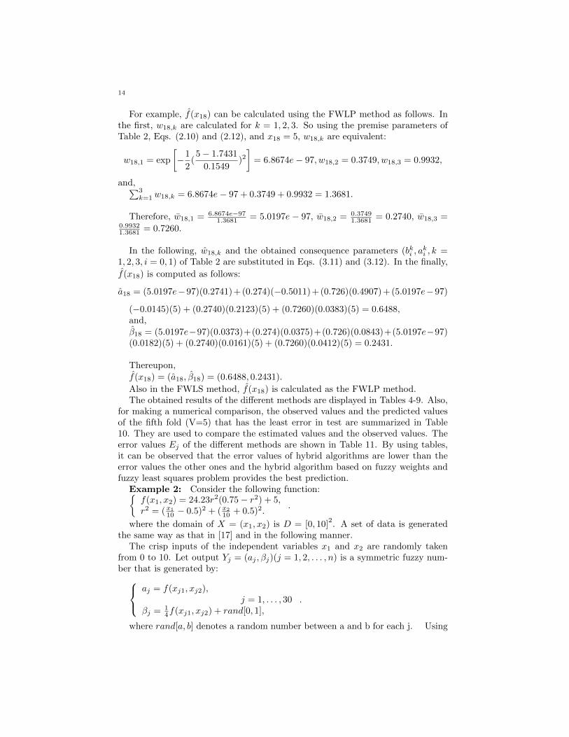
for making a numerical comparison, the observed values and the predicted valuesof the fifth fold (V=5) that has the least error in test are summarized in Table10. They are used to compare the estimated values and the observed values. Theerror values Ej of the different methods are shown in Table 11. By using tables,it can be observed that the error values of hybrid algorithms are lower than theerror values the other ones and the hybrid algorithm based on fuzzy weights andfuzzy least squares problem provides the best prediction.

Example 2: Consider the following function:{f(x1, x2) = 24.23r2(0.75− r2) + 5,r2 = (x1

10 − 0.5)2 + (x2

10 + 0.5)2..

where the domain of X = (x1, x2) is D = [0, 10]2. A set of data is generated

the same way as that in [17] and in the following manner.The crisp inputs of the independent variables x1 and x2 are randomly taken

from 0 to 10. Let output Yj = (aj , βj)(j = 1, 2, . . . , n) is a symmetric fuzzy num-ber that is generated by: aj = f(xj1, xj2),

j = 1, . . . , 30βj = 1

4f(xj1, xj2) + rand[0, 1],.

where rand[a, b] denotes a random number between a and b for each j. Using

15


xj Ej Ej Ej Ej

of FWLS method of FWLP method of QP method of LP method

0.75 0.0166 0.0694 0.1078 0.1110

1.25 0.0324 0.0302 0.0860 0.0888

1.50 0.0438 0.0478 0.1020 0.1049

2 0.0131 0.0405 0.1463 0.1473

2.25 0.0100 0.0319 0.1700 0.1697

2.50 0.0343 0.0072 0.0722 0.0726

2.75 0.0437 0.0550 0.1778 0.1778

3.00 0.0037 0.0510 0.1792 0.1795

3.25 0.0422 0.0719 0.1775 0.1779

3.5 0.0934 0.0951 0.2455 0.2459

3.75 0.0610 0.0513 0.1671 0.1673

4 0.0896 0.0579 0.1584 0.1581

4.25 0.0483 0.1092 0.2124 0.2123

4.75 0.0905 0.1686 0.2031 0.2023

5.00 0.0950 0.0034 0.1212 0.1183

5.25 0.0387 0.1260 0.1609 0.1583

Test data

1.00 0.0442 0.0357 0.0638 0.0676

1.75 0.0560 0.0544 0.1005 0.1027

4.50 0.0209 0.1031 0.1766 0.1761

Table 12. The obtained premise and consequence parameters of theFWLP method.

k (τk, σk) (bk0 , αk0) (bk1 , α

k1) (bk2 , α

k2)

1 (-0.1313,1.0728) (-8.6242,1.0819) (2.3234,0.3206) (2.8434,0.0797)

2 (10.2741,1.7615) (-18.5882,0.4728) (1.1806,0.6415) (1.9722,0.0711)

3 (1.6331,4.3634) (-5.2832,1.5163 ) (2.4173,0.2220) (-0.6884,0.2267)

4 (11.3822,4.0364) (17.3542,1.0915) (0.9686,0.3688) (-0.8430,0.0349)

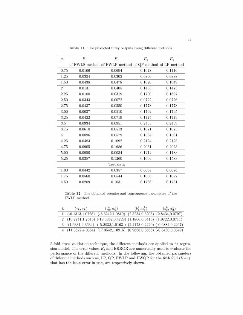
5-fold cross validation technique, the different methods are applied to fit regres-sion model. The error values Ej and ERROR are numerically used to evaluate theperformance of the different methods. In the following, the obtained parametersof different methods such as, LP, QP, FWLP and FWQP for the fifth fold (V=5),that has the least error in test, are respectively shown.

16

Table 13. The obtained premise and consequence parameters of theFWLS method.

k (τk, σk) (bk0 , αk0) (bk1 , α

k1) (bk2 , α

k2)

1 (-0.1313,1.0728) (-10.0164,3.4735) (2.5053,0.2557) (3.295,-0.7969)

2 (10.2741,1.7615) (-24.3085,8.1058) (1.1930,0.4945) (2.4987,0.6068)

3 (1.6331,4.3634) (-3.9404,0.0396) (2.1887,0.4699) (-0.5228,-0.3314)

4 (11.3822,4.0364) (15.1877,10.5082) (1.1195,0.2425) (-0.7718, 0.8392)

Table 14. The obtained error results of the first fold.



FWLS 0.2507 3.2065 10.3372 8.7480

FWLP 0.8923 2.5053 15.4732 7.7833

QP 4.2831 5.6830 35.4783 9.8158

LP 4.7131 5.8636 36.8859 10.1274

Table 15. The obtained error results of the second fold.



FWLS 0.6737 1.3293 15.0116 6.0966

FWLP 1.7938 4.5294 19.9959 9.3311

QP 4.5529 4.6121 36.1482 9.1455

LP 4.7448 5.0400 36.9513 9.5492

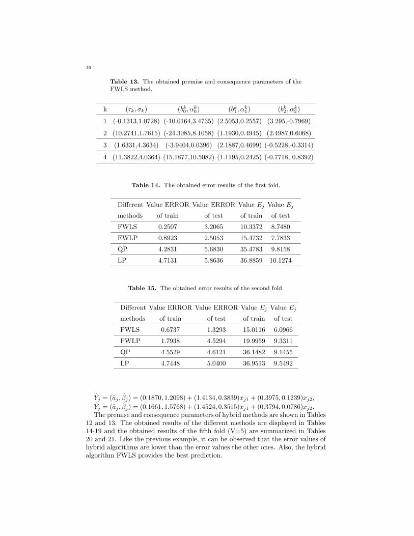
Yj = (aj , βj) = (0.1870, 1.2098) + (1.4134, 0.3839)xj1 + (0.3975, 0.1239)xj2,

Yj = (aj , βj) = (0.1661, 1.5768) + (1.4524, 0.3515)xj1 + (0.3794, 0.0786)xj2.The premise and consequence parameters of hybrid methods are shown in Tables

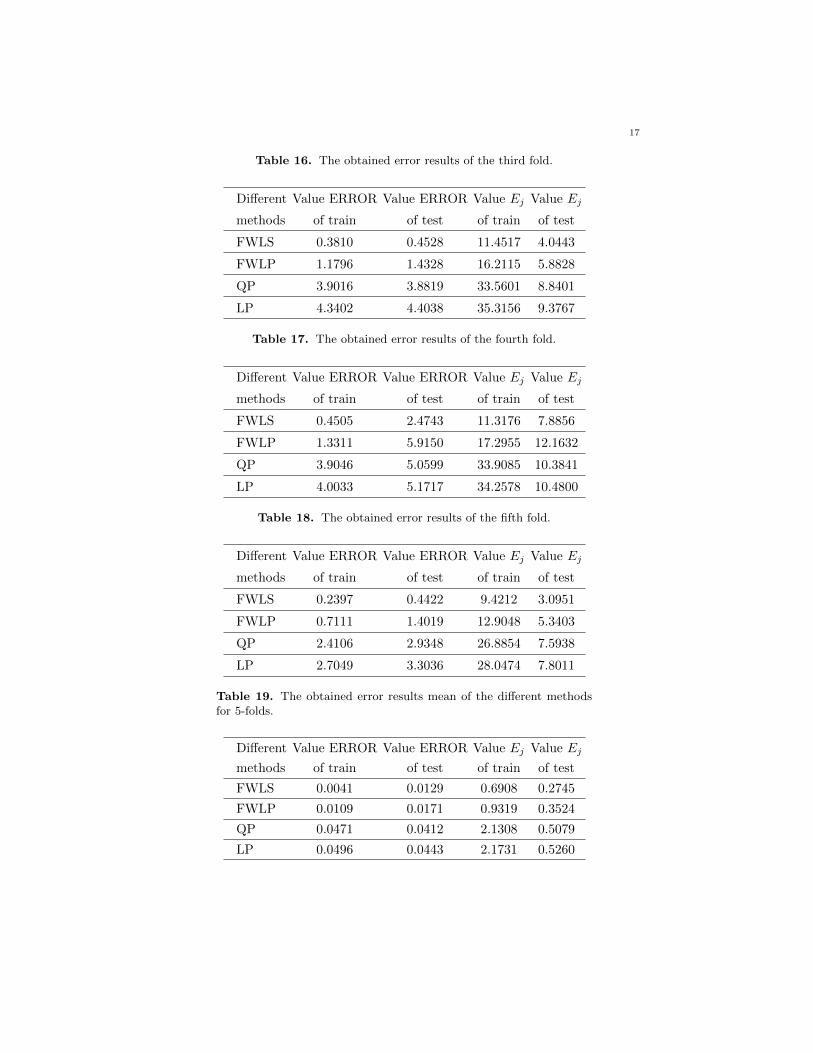
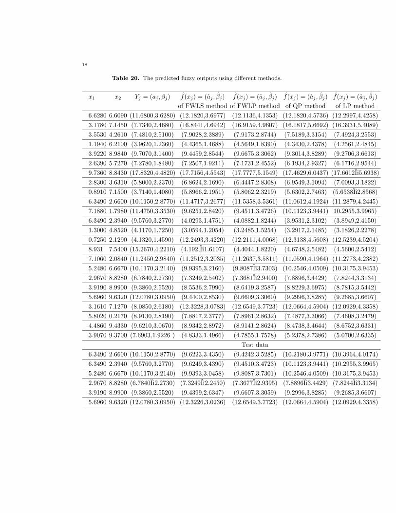
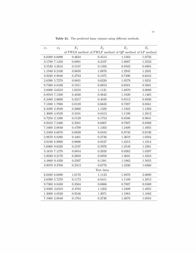
12 and 13. The obtained results of the different methods are displayed in Tables14-19 and the obtained results of the fifth fold (V=5) are summarized in Tables20 and 21. Like the previous example, it can be observed that the error values ofhybrid algorithms are lower than the error values the other ones. Also, the hybridalgorithm FWLS provides the best prediction.

17

Table 16. The obtained error results of the third fold.



FWLS 0.3810 0.4528 11.4517 4.0443

FWLP 1.1796 1.4328 16.2115 5.8828

QP 3.9016 3.8819 33.5601 8.8401

LP 4.3402 4.4038 35.3156 9.3767

Table 17. The obtained error results of the fourth fold.



FWLS 0.4505 2.4743 11.3176 7.8856

FWLP 1.3311 5.9150 17.2955 12.1632

QP 3.9046 5.0599 33.9085 10.3841

LP 4.0033 5.1717 34.2578 10.4800

Table 18. The obtained error results of the fifth fold.



FWLS 0.2397 0.4422 9.4212 3.0951

FWLP 0.7111 1.4019 12.9048 5.3403

QP 2.4106 2.9348 26.8854 7.5938

LP 2.7049 3.3036 28.0474 7.8011

Table 19. The obtained error results mean of the different methodsfor 5-folds.



FWLS 0.0041 0.0129 0.6908 0.2745

FWLP 0.0109 0.0171 0.9319 0.3524

QP 0.0471 0.0412 2.1308 0.5079

LP 0.0496 0.0443 2.1731 0.5260

18


x1 x2 Yj = (aj , βj) f(xj) = (aj , βj) f(xj) = (aj , βj) f(xj) = (aj , βj) f(xj) = (aj , βj)


6.6280 6.6090 (11.6800,3.6280) (12.1820,3.6977) (12.1136,4.1353) (12.1820,4.5736) (12.2997,4.4258)

3.1780 7.1450 (7.7340,2.4680) (16.8441,4.6942) (16.9159,4.9607) (16.1817,5.6692) (16.3931,5.4089)

3.5530 4.2610 (7.4810,2.5100) (7.9028,2.3889) (7.9173,2.8744) (7.5189,3.3154) (7.4924,3.2553)

1.1940 6.2100 (3.9620,1.2360) (4.4365,1.4688) (4.5649,1.8390) (4.3430,2.4378) (4.2561,2.4845)

3.9220 8.9840 (9.7070,3.1400) (9.4459,2.8544) (9.6675,3.3062) (9.3014,3.8289) (9.2706,3.6613)

2.6390 5.7270 (7.2780,1.8480) (7.2507,1.9211) (7.1731,2.4552) (6.1934,2.9327) (6.1716,2.9544)

9.7360 8.8430 (17.8320,4.4820) (17.7156,4.5543) (17.7777,5.1549) (17.4629,6.0437) (17.6612Iı5.6938)

2.8300 3.6310 (5.8000,2.2370) (6.8624,2.1690) (6.4447,2.8308) (6.9549,3.1094) (7.0093,3.1822)

0.8910 7.1500 (3.7140,1.4080) (5.8966,2.1951) (5.8062,2.3219) (5.6302,2.7463) (5.6538Iı2.8568)

6.3490 2.6600 (10.1150,2.8770) (11.4717,3.2677) (11.5358,3.5361) (11.0612,4.1924) (11.2879,4.2445)

7.1880 1.7980 (11.4750,3.3530) (9.6251,2.8420) (9.4511,3.4726) (10.1123,3.9441) 10.2955,3.9965)

6.3490 2.3940 (9.5760,3.2770) (4.0293,1.4751) (4.0882,1.8244) (3.9531,2.3102) (3.8949,2.4150)

1.3000 4.8520 (4.1170,1.7250) (3.0594,1.2054) (3.2485,1.5254) (3.2917,2.1485) (3.1826,2.2278)

0.7250 2.1290 (4.1320,1.4590) (12.2493,3.4220) (12.2111,4.0068) (12.3138,4.5608) (12.5239,4.5204)

8.931 7.5400 (15.2670,4.2210) (4.192,Iı1.6107) (4.4044,1.8220) (4.6748,2.5482) (4.5600,2.5412)

7.1060 2.0840 (11.2450,2.9840) (11.2512,3.2035) (11.2637,3.5811) (11.0590,4.1964) (11.2773,4.2382)

5.2480 6.6670 (10.1170,3.2140) (9.9395,3.2160) (9.8087Iı3.7303) (10.2546,4.0509) (10.3175,3.9453)

2.9670 8.8280 (6.7840,2.2730) (7.3249,2.5402) (7.3681Iı2.9400) (7.8896,3.4429) (7.8244,3.3134)

3.9190 8.9900 (9.3860,2.5520) (8.5536,2.7990) (8.6419,3.2587) (8.8229,3.6975) (8.7815,3.5442)

5.6960 9.6320 (12.0780,3.0950) (9.4400,2.8530) (9.6609,3.3060) (9.2996,3.8285) (9.2685,3.6607)

3.1610 7.1270 (8.0850,2.6180) (12.3228,3.0783) (12.6549,3.7723) (12.0664,4.5904) (12.0929,4.3358)

5.8020 0.2170 (8.9130,2.8190) (7.8817,2.3777) (7.8961,2.8632) (7.4877,3.3066) (7.4608,3.2479)

4.4860 9.4330 (9.6210,3.0670) (8.9342,2.8972) (8.9141,2.8624) (8.4738,3.4644) (8.6752,3.6331)

3.9070 9.3700 (7.6903,1.9226 ) (4.8333,1.4966) (4.7855,1.7578) (5.2378,2.7386) (5.0700,2.6335)

Test data

6.3490 2.6600 (10.1150,2.8770) (9.6223,3.4350) (9.4242,3.5285) (10.2180,3.9771) (10.3964,4.0174)

6.3490 2.3940 (9.5760,3.2770) (9.6249,3.4390) (9.4510,3.4723) (10.1123,3.9441) (10.2955,3.9965)

5.2480 6.6670 (10.1170,3.2140) (9.9393,3.0458) (9.8087,3.7301) (10.2546,4.0509) (10.3175,3.9453)

2.9670 8.8280 (6.7840Iı2.2730) (7.3249Iı2.2450) (7.3677Iı2.9395) (7.8896Iı3.4429) (7.8244Iı3.3134)

3.9190 8.9900 (9.3860,2.5520) (9.4399,2.6347) (9.6607,3.3059) (9.2996,3.8285) (9.2685,3.6607)

5.6960 9.6320 (12.0780,3.0950) (12.3226,3.0236) (12.6549,3.7723) (12.0664,4.5904) (12.0929,4.3358)

19


x1 x2 Ej Ej Ej Ej


6.6280 6.6090 0.3634 0.4514 1.1563 1.0756

3.1780 7.1450 0.0881 0.2107 1.0887 1.2523

3.5530 4.2610 0.5187 0.1492 0.8502 0.8905

1.1940 6.2100 0.8658 1.0876 1.2945 1.2831

3.9220 8.9840 0.2783 0.1075 0.7496 0.6244

2.6390 5.7270 0.0831 0.6228 1.9579 1.9231

9.7360 8.8430 0.1911 0.0853 0.6501 0.5601

2.8300 3.6310 1.0210 1.1131 1.8870 2.0009

0.8910 7.1500 0.4040 0.3842 1.1820 1.1465

6.3490 2.6600 0.3317 0.4828 0.8512 0.8940

7.1880 1.7980 0.8189 0.6633 0.7287 0.8561

6.3490 2.3940 0.2660 1.1328 1.1924 1.1203

1.3000 4.8520 0.3101 0.8413 1.1189 1.2812

0.7250 2.1290 0.5129 0.1753 0.8586 0.9041

8.9310 7.5400 0.3501 0.6867 0.7807 0.8569

7.1060 2.0840 0.4799 1.1202 1.2409 1.4955

5.2480 6.6670 0.0839 0.0434 0.8748 0.9136

2.9670 8.8280 0.4401 0.2730 1.3678 1.0584

3.9190 8.9900 0.9696 0.8537 1.2315 1.1814

5.6960 9.6320 0.2197 0.5976 1.2549 1.2361

3.1610 7.1270 0.0854 0.2028 0.9262 1.0207

5.8020 0.2170 0.2682 0.8050 1.3031 1.3310

4.4860 9.4330 0.2397 0.1381 1.1062 1.5055

3.9070 9.3700 0.2313 0.6770 1.2330 1.6360

Test data

6.6280 6.6090 1.0170 1.1123 1.8870 2.0009

2.6390 5.7270 0.1173 0.8411 1.1189 1.2812

9.7360 8.8430 0.3504 0.6866 0.7807 0.8569

2.8300 3.6310 0.4794 1.1202 1.2409 1.4955

1.3000 4.8520 0.9546 1.3071 1.1984 1.1082

7.1060 2.0840 0.1764 0.2730 1.3678 1.0584

20

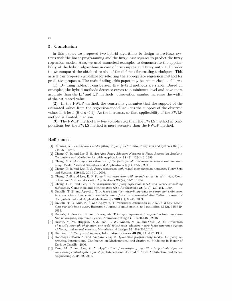
5. Conclusion

In this paper, we proposed two hybrid algorithms to design neuro-fuzzy sys-tems with the linear programming and the fuzzy least squares to predict the fuzzyregression model. Also, we used numerical examples to demonstrate the applica-bility of the hybrid algorithms in case of crisp inputs and fuzzy output. In orderto, we compared the obtained results of the different forecasting techniques. Thisarticle can propose a guideline for selecting the appropriate regression method forpredictive proposes. The main findings this paper may be summarized as follows:

(1). By using tables, it can be seen that hybrid methods are stable. Based onexamples, the hybrid methods decrease errors to a minimum level and have moreaccurate than the LP and QP methods. observation number increases the widthof the estimated value

(2). In the FWLP method, the constrains guarantee that the support of theestimated values from the regression model includes the support of the observedvalues in h-level (0 < h ≤ 1). As the increases, so that applicability of the FWLPmethod is limited in action.

(3). The FWLP method has less complicated than the FWLS method in com-putations but the FWLS method is more accurate than the FWLP method.

References

[1] Celmins, A. Least-squares model fitting to fuzzy vector data, Fuzzy sets and systems 22 (3),245-269, 1987.

[2] Cheng, C.-B. and Lee, E. S. Applying Fuzzy Adoptive Network to Fuzzy Regression Analysis,

Computers and Mathematics with Applications 38 (2), 123-140, 1999.[3] Cheng, M.Y. An improved estimator of the finite population mean in simple random sam-

pling, Model Assisted Statistics and Applications 6 (1), 47-55, 2011.

[4] Cheng, C.-B. and Lee, E. S. Fuzzy regression with radial basis function networks, Fuzzy Setsand Systems 119 (3), 291-301, 2001.

[5] Cheng, C.-B. and Lee, E. S. Fuzzy linear regression with spreads unrestricted in sign, Com-

puters and Mathematics with Applications 28 (4), 61-70, 1994.[6] Cheng, C.-B. and Lee, E. S. Nonparametric fuzzy regression k-NN and kernel smoothing

techniques, Computers and Mathematics with Applications 38 (3-4), 239-251, 1999.

[7] Dalkilic, T. E. and Apaydin, T. A fuzzy adaptive network approach to parameter estimationin cases where independent variables come from an exponential distribution, Journal of

Computational and Applied Mathematics 233 (1), 36-45, 2009.[8] Dalkilic, T. E. Kula, K. S. and Apaydin, T. Parameter estimation by ANFIS Where depen-

dent variable has outlier, Hacettepe Journal of mathematics and statistics, 43 (2), 315-329,

2014.[9] Danesh, S. Farnoosh, R. and Razzaghnia, T Fuzzy nonparametric regression based on adap-

tive neuro-fuzzy inference system, Neurocomputing 173, 1450-1460, 2016.

[10] Dewan, M. W. Huggett, D. J. Liao, T. W. Wahab, M. A. and Okeil, A. M. Predictionof tensile strength of friction stir weld joints with adaptive neuro-fuzzy inference system

(ANFIS) and neural network, Materials and Design 92, 288-299,2016.

[11] Diamond, P. Fuzzy least squares, Information Sciences 46 (3), 141-157, 1988.[12] Donoso, S. Marin N. and Amparo Vila, M. Quadratic programming models for fuzzy re-

gression, International Conference on Mathematical and Statistical Modeling in Honor of

Enrique Castillo, 2006.[13] Fang, M. C. and Lee, Zi. Y. Application of neuro-fuzzy algorithm to portable dynamic

positioning control system for ships, International Journal of Naval Architecture and Ocean

Engineering 8, 38-52, 2016.

21

[14] Farnoosh, R. Ghasemian, J. and Solaymani fard, O. A modification on ridge estimation for

fuzzy nonparametric regression, Iranian Journal of Fuzzy System 9 (2), 75-88, 2012.

[15] Gaxiola, F. Melin, P. Valdez, F. Castro, J. R. and Castillo, O. Optimization of type-2 fuzzyweights in back propagation learning for neural networks using GAs and PSO, Applied Soft

Computing 38, 860OCo871, 2016.[16] Ishibuchi, H. Kwon, K. and Tanaka, H. A learning algorithm of fuzzy neural networks with

triangular fuzzy weights, Fuzzy Sets and Systems 71 (3), 277-293, 1995.

[17] Ishibushi, H. Tanaka, H. and Okado, H. An architecture of neural networks with intervalweights and its application to fuzzy regression analysis, Fuzzy Sets and Systems 57 (1),27-39,

1993.

[18] Ishibushi, H. and Tanaka, H. Fuzzy regression analysis using neural networks, Fuzzy Setsand systems 50 (3), 257-265, 1992.

[19] Jang, J.S.R. Self-learning fuzzy controllers based on temporal back-propagation, IEEE

Transactions on Neural Network , IEEE Transactions on Neural Network 3, 714-723, 1992.[20] Jang, J.S.R. ANFIS: adaptive-network-based fuzzy inference system, IEEE Trans Syst Man

Cyber 23 (3), 665-685, 1993.

[21] Kayacan, E. and Khanesar, M. A. Chapter 8 OCo Hybrid Training Method for type-2 fuzzy

Neural networks using particle swarm optimization, Fuzzy Neural Networks for Real Time

Control Applications, 133OCo160, 2016.

[22] Kim, B. and Bishu, R. R. Evaluation of fuzzy linear regression models by comparing mem-

bership functions, Fuzzy Sets and Systems 100 (1-3), 343-351, 1998.[23] Kiraly, A. Fogarassy, A. V. and Abonyi, J. Geodesic distance based fuzzy c-medoid clustering

OCo searching for central points in graphs and high dimensional data, Fuzzy Sets and

Systems 286 , 157OCo172, 2016.

[24] Ming, M. Friedman, M. and Kandel, A. General fuzzy least squares, Fuzzy Sets and Systems

88 (1), 107OCo118, 1997.

[25] Mosleh, M. Otadi, M. and abbasbandy, S. Evaluation of fuzzy regression model by fuzzyneural networks, Journal of Computational and Applied Mathematics 234 (1), 825- 834,

2010.[26] Mosleh, M. Fuzzy neural network for solving a system of fuzzy differential equations, Applied

Soft Computing 13, 3597-3607, 2013.

[27] Nasrabadi, M.M. and Nasrabadi, E. A. mathematical-programming approach to fuzzy linearregression analysis, Applied Mathematics and Computation 155 (3), 873-881, 2004.

[28] Pasha, E. Razzaghnia, T. Allahviranloo, T. Yari, Gh. and Mostafaei, H. R. A new math-

ematical programming approach in fuzzy linear regression models, Applied MathematicalSciences 35, 1715, 2007.

[29] Razzaghnia, T. Danesh, S.and Maleki, A. Hybrid fuzzy regression with trapezoidal fuzzy

data, Proc. SPIE 8349 (834921), 2011.[30] Razzaghnia, T. and Danesh, S. Nonparametric Regression with Trapezoidal Fuzzy Data,

International Journal on Recent and Innovation Trends in Computing and Communication

(IJRITCC) 3 (6), 3826 OCo 3831, 2015.

[31] Sarhadi, P. Rezaie, B. and Rahmani, Z. Adaptive predictive control based on adaptive neuro-

fuzzy inference system for a class of nonlinear industrial processes, Journal of the TaiwanInstitute of Chemical Engineers 61, 132-137, 2016.

[32] Shapiro, A. The merge of neural networks, fuzzy logic, and genetic algorithms, Insurance:

Mathematics and Economics 31 (1), 115-131, 2002.[33] Sridevi, S. and Nirmal, S. ANFIS based decision support system for prenatal detection of

Truncus Arteriosus congenital heart defect, Applied Soft Computing 46, 577OCo587, 2016.

[34] Stone, M. Cross validation choice and assessment of statistical predictions, Journal of theRoyal Statistical Society 36 (series B), 111-147, 1974.

[35] Takagi, T. and Sugeno, M. Fuzzy identification of systems and its application to modelling

and control, IEEE Transactions on Systems, Man and Cybernetics 15, 116-132, 1985.

[36] Tanaka, H. Fuzzy data analysis by possibilistic linear models, Fuzzy Sets and Systems 24(3), 363-375, 1987.

22

[37] Tanaka, H. Hayashi, I. and Watada, J. Possibilistic linear regression analysis for fuzzy data,

European Journal of Operational Research 40 (3), 389-396, 1989.

[38] Tanaka, H. and Watada, J. Possibilistic linear systems and their application to the linearregression model, Fuzzy Sets and Systems 27 (3), 275-289, 1988.

[39] Tanaka, H. Uejima, S. K. and Asia, K. Linear regression analysis with fuzzy model, IEEE

Transactions on Systems, Man and Cybernetics 12, 903-907, 1982.[40] Wang, N. Zhang, W. X. and Mei, C. L. Fuzzy nonparametric regression based on local linear

smoothing technique,Information Sciences 177 (18), 3882-3900, 2007.

[41] Zhang, P. Model selection via multifold cross validation, Annals of Statistics 21 (1),299-313, 1993.

fuzzy parameters estimation via hybrid...

Documents