fuzzy logic, control and optimisation
TRANSCRIPT

Fuzzy Logic, Control, and timisation
A Thesis
submitted in partial fulfilment
of the requirements for the Degree
of
Master of Engineering (Mechanical)
in the
University of Canterbury
by
W. J. Hoyle RE.
University of Canterbury
1996

Abstract
This thesis examines the utility of fuzzy logic in the field of control engineering. A tutorial
introduction to the field offuzzy control is presented during the development of an efficient
fuzzy controller. Using the controller as a starting point, a set of criteria are developed that
ensure a close connection between rule base construction and control surface geometry. The
properties of the controller are exploited in the design of a global controller optimiser based
on a genetic algorithm, and a tutorial explaining how the optimiser may be used to effect
automatic controller design is given. A library of software that implements a fast fuzzy
controller, a genetic algorithm, and various utility routines is included.

Acknowledgments
I wish to thank: my supervisor O.R. Dunlop and my parents, Steve and Cheryl Hoyle, for their support and encouragement during the writing of this thesis.

Cont nts 1. Introduction ............ 111111 ••••••••••••••••••••••••••••••••••••••••••••••••••••••• 1 1.1 Description ................................................................. 1 1.2 Fuzzy Logic and Control Engineering ......................... 1 1.2.1 Some Limitations of Modern Control Methods .... 1 1.2.2 An Alternative: Rule Based Control ..................... 2 1.3 An Outline of this Thesis ............................................. 2
2. Basic Fuzzy Logic ............................................................ 4 2.1 The Fuzzy Rule Base ................................................. 4 2.2 Fuzzy Sets .................................................................. 6 2.2.1 Membership functions ......................................... 6 2.2.2 Fuzzy Relations ................................................... 7 2.2.3 Height .................................................................. 8 2.2.4 Support ................................................................ 8 2.2.5 Core .................................................................... 8 2.2.6 Fuzzy Partitions ................................................... 8 2.3 Operations on Fuzzy Sets .......................................... 9 2.3.1 Union and Intersection ........................................ 9 2.3.2 Degree of Matching ........................................... 10 2.3.3 Projection .......................................................... 10 2.3.4 Cylindrical Extension .......................................... 11 2.3.4 Composition ....................................................... 11 2.4 Fuzzy Rules ............................................................ " ... 11 2.4.1 Fuzzy Connectives ............................................. 11 2.4.2 Fuzzy Implication .............................................. 12 2.4.3 Reasoning with a Fuzzy Rule ............................ 12 2.5 An Example of Inference with a Fuzzy Rule ............. 13 2.6 The Fuzzy Rule Base ............................................... 16 2.6.1 Reasoning with a Fuzzy Rule Base ................... 16 2.6.2 The Completeness of a Rule Base ................... 17 2.7 Example Continued .................................................. 17 2.8 Defuzzi"fication .......................................................... 19 2.8.1 Maximum-Membership Defuzzification ............. 19 2.8.2 Centroidal Defuzzification ................................. 19 2.8.3 Consequent Set Modelling ................................ 21 2.9 Summary .................................................................. 23
3. Fuzzy Rule Base Design ............................................... 24 3.1 Rule Base Legibility .................................................. 24 3.2 The Well Conditioned Rule Base .............................. 25

3.2.1 Rules as Points on a Control Surface ............... 25 3.2.2 Output Set Weighting ........................................ 27 3.2.4 Writing a Well Conditioned Rule Base .............. 31 3.3 Writing a Rule Base for a Fuzzy Controller .............. 31 3.3.1 Choice of control variables ................................ 32 3.3.2 Input Set Design ................................................ 32 3.3.3 Rule Design ....................................................... 32 3.3.4 Output Set Weighting ........................................ 32 3.3.5 Performance Tuning .......................................... 33 3.3.6 Rule Base Tuning .............................................. 33 3.4 Traditional Design Methods and Fuzzy Logic ........... 34 3.5 Global Optimisation Methods ................................... 34 3.6 Combining Methods .................................................. 34 3.7 Stability ..................................................................... 35 3.8 Summary .................................................................. 35
4. The Optimisation of a Fuzzy Controller ....................... 37 4.1 Fuzzy logic and Genetic Algorithms ......................... 38 4.2 Genetic Algorithms ................................................... 40 4.2.1 The SGA Chromosome ..................................... 41 4.2.2 The SGA Population ......................................... 41 4.2.2 The SGA Evaluation Function ........................... 41 4.2.3 The SGA Generation Function .......................... 42 4.2.4 The SGA Selection Function ............................. 43 4.2.5 The SGA Crossover Function ........................... 43 4.2.6 The SGA Mutation Function .............................. 43 4.3 Some Properties of the SGA .................................... 44 4.4 An Efficient Parameterisation of a Fuzzy Controller. 44 4.5 Incorporating Expert Knowledge .............................. 46 4.6 Summary .................................................................. 46
5. The Design of a Fuzzy Inference Engine ..................... 48 5.1 Design concerns ....................................................... 48 5.2 Representing Fuzzy Sets in C .................................. 48 5.3 Representing Fuzzy Rules in C ................................ 49 5.4 Possible Optimisations ............................................. 51 5.5 Summary .................................................................. 51
6. Example: Velocity Control of a Variable Pitch Fan ..... 52 6.1 A Simple Model of a Variable Pitch Propeller ........... 52 6.2 The Control Problem ................................................ 54 6.2.1 Input Sensor ...................................................... 54 6.2.2 Sampling Period ................................................ 54

6.2.3 Output ............................................................... 54 6.2.4 The Task ............................................................ 55 6.3 A Fuzzy Controller .................................................... 55 6.3.1 Input Set Design ................................................ 55 6.3.2 The Rule Base .................................................. 57 6.4 Optimisation of the Controller ................................... 58 6.4.1 Incorporation of Expert Knowledge ................... 59 6.4.2 The Main Loop .................................................. 59 6.4.3 The Fitness Fu nction ......................................... 60 6.4.4 The Optimisation Run ....................................... 64 6.5 Results ..................................................................... 65 6.6 Examination of Results ............................................. 66 6.6.1 Calculating Rule Usage ..................................... 66 6.6.2 Rule Reduction .................................................. 67 6.7 Discussion ................................................................ 69
7. Conclusion .................................... It- •••••••••••••••••••••••••••••••• 71 7.1 Suggested Further Work .......................................... 72
References ........................................... " ...... 111 ••• IIIII •• IS •••••••••••••••••••••••••• 73
A. Software .......................................................................... 76
1
This thesis examines both fuzzy logic and genetic algorithms, discusses the possibili
ties inherent in the combination of the two technologies, and describes the develop
ment of software to implement them in conjunction with each other.
Fuzzy logic has a wide variety of applications. This thesis examines the use of fuzzy
logic methods in control.
1.1 Description
Fuzzy Logic was developed by Zadeh (1965) to provide a set of tools for manipulating
imprecise data. Since its introduction, fuzzy logic has been applied in many areas,
some of which include: systems analysis, signal processing, pattern recognition,
decision analysis, diagnostics, and controL
Fuzzy logic was first introduced to the area of control by Mamdani (1975), with the
intent of duplicating the behaviour of human system operators. Imprecise descrip
tions of a control task that are obtained from operators can be modelled with fuzzy
logic, allowing automated control without the need for a formal analysis of the
system.
Discussion of fuzzy technology is limited to the calculus of fuzzy if/then rules (CFR)
for purposes of concision and clarity; from Zadeh (1992):
The calculus offuzzy if/then rules is simple and close to intuition. Furthermore, it is largely self contained and does not require an extensive familiarity with fuzzy logic.
Controllers can be designed and built from the tools of CFR.
1.2 Fuzzy Logic and Control Engineering
On the most abstract level, all controllers are simply mapping functions-they map
their inputs and their state to their outputs. S tandard controllers do this computationally;
fuzzy logic controllers use a rule base.
1.2.1 Some limitations of Modern Control Methods
The majority of the literature on modern control methods concerns linear control.
Nonlinear problems are usually dealt with by approximating them with a linear

2
model. Those solutions that do address nonlinear problems lack generality; they are
only applicable to a specific type of problem.
1.2.2 An Alternative: Rule Based Control
Fuzzy logic may be viewed as a language for describing arbitrary control surfaces. As
such, it is not restricted, as classical controllers are, to the description oflinear control
surfaces, and it is not restricted by the complexities of nonlinear math, as some
possible solutions to the control of nonlinear systems are.
1.3 An Outline of this Thesis
Since the introduction of fuzzy logic to the field of control engineering, many
variations on the basic design of fuzzy controllers have been presented. Proceeding
from the point of view that a practical design should lead to a fast, compact
representation on a microcontroller, chapter 2 begins with an introduction to the
calculus of fuzzy rules. The standard simplifications to the theory are presented and
controller design that takes advantage of several less well known optimisations is
described.
If fuzzy logic is viewed as a language for describing control surfaces, then the utility
of any definition of a fuzzy controller is determined not only by the speed and
compactness of the resulting code, but additionally by how easily a control surface
can be built using it. Chapter 3 addresses a problem in the traditional design
methodology of fuzzy controllers - discussion in the current literature invariably
fails to address the connection between fuzzy rule bases and the control surfaces that
they describe; given a fuzzy rule base there is no way to discover the geometry of the
control surface (other than by extensive calculation), and given a control surface there
is no way that a defining rule base can be built easily.
A set of criteria, referred to as "the well conditioned rule base," that enable the
construction of rule bases with a strong connection to their control surfaces is defined,
and methods of determining control surface geometry are presented. The chapter
concludes with a description of the traditional method offuzzy controller design from
the point of view of the well conditioned rule base.
In chapter 4 it is noted that the traditional method of fuzzy controller design can be
viewed as a hand optimisation scheme. Design consists of iterated testing and
adjustment, which is conducted until a solution is found. A summary of other
optimisation design techniques is presented, and it is noted that fuzzy logic has
particular promise in the field of computer aided controller design because 1) it allows

3
an arbitrary control surface and 2) the result of optimisation is presented in an easily
understandable form (that is, a set of simple, English-like rules).
A survey of the various global optimisation schemes that have been used with fuzzy
logic is presented and it is noted that particular attention has been paid to the use of
genetic algorithms. Using the well conditioned rule base as a model, it is shown that
previous schemes have used inefficient parameterisations of the fuzzy controllers that
they optimised. An introduction to the use of genetic algorithms is presented, and an
efficient parameterisation of a fuzzy controller (based on the well conditioned rule
base) is developed. Software that implements a simple genetic algorithm was written
to test these ideas. Listings appear in appendix A.
Chapter 5 describes the development of efficient fuzzy controller software that
implements the controller design developed in chapter 2 and makes use of several
optimisations that the well conditioned rule base makes possible.
The concluding chapter contains a tutorial that shows how the software in appendix
A may be used to automatically design a controller (specifically, a speed controller
for a variable pitch propeller), and demonstrates the utility ofthe well conditioned rule
base.

4
The following is a brief introduction to the calculus of fuzzy rules. It includes only
those parts of fuzzy theory that will be used in this thesis. A more comprehensive
introduction can be found in Jager (1995) and Kruse (1994).
2.1 The Fuzzy Rule Base
Traditional rule bases are bivalent. If a controller is implemented with a bivalent rule
base, the control surface generated will suffer from heavy quantisation. As an
example, consider a set of rules for stopping a car:
In this rule base the speed of the car is represented by the variable s (in km/h), where
s is in the set S of applicable car velocities: S = {s I S E [0,180]}.
The variable d (in metres) represents the position of the car relative to the point where
it must be stopped; d is in the set D of applicable stopping distances: D = (d IdE
[0,140]).
Braking effort (a percentage of maximum possible braking effort) is represented by
the variable b.
Partition S into the following subsets: slow = [0,10), med = [10, 50), fast = [50, 80]
Partition D into the following subsets: short = [0 ,30), mid = [30, 100), long = [100, 140]
Now, define some rules:
if s is fast and d is long then b is 50% if s is fast and d is mid then b is 100% if s is fast and d is short then b is 100% if s is med and d is long then b is 50% if s is med and d is mid then b is 50% if s is med and d is short then b is 100% if s is slow and d is long then b is 5% if s is slow and d is mid then b is 5% if s is slow and d is short then b is 50%
Table 2.1 Rule Base For Stopping a Car.
Note that the subsets ofS fom1 apartition, as do the subsets ofD. If they did not, the

5
rule base might be ambiguous; if some of the sets intersected it would be possible for
two or more contradictory rules to be true at the same time (for example, if the speed
was fast, and the distance fell somewhere in the intersection of mid and long, the first
and second rules would contradict); if some elements of S or D were not included in
any of the subsets, the rule base would not produce any corresponding output for
them.
The control surface that this rule base defines appears in figure 2.1. Obviously, the
coarse surface pictured will not result in good control- it is unlikely that the car will
stop at the desired point.
80
Velocity
'---------~C----.. 40 (km/h)
140
BrakIng Effort
(%)
Figure 2.1: Control sUrface generated by a bivalent rule base
The stepped surface is not bad in itself - quantisation is always a factor in digital
control but the size of the bivalent rule base needed to gain adequate resolution
for good control would be prohibitive.
One solution to this problem is to use fuzzy logic. The central idea of fuzzy logic is
that membership in sets may be partial; the practical effect of this concept is a
smoother control surface. A fuzzy logic controller may be viewed as a combination
of a bivalent rule base and an interpolative mechanism.
Figure 2.2 shows a non-quantised control surface generated by the fuzzy equivalent
of the bivalent rule base in table 1. The process of fuzzy control is explained in the
next section.

140 Distance
(m)
80
(%)
Figure 2.2 Control surface generated by afuzzy rule base
2.2 Fuzzy Sets
6
A problem arises when classical sets are used to model vague concepts like "a
medium velocity." The classification ofvelocities into the setmed is difficult because
it is not obvious which velocities belong to the set. Is 10 km/h a medium velocity? If
it is, is then 9.99 km/h a medium velocity? A distinction between med and not med
must be made somewhere, so at some point a group of very similar velocities must
be divided into two differing classifications.
Fuzzy logic addresses this problem by allowing graded set membership. All elements
of a fuzzy set have a membership grade in the interval [0,1]. The interval [0,1]
corresponds to the truth set {O, I} used in bivalent logic (where 1 means true and ° means false). So while 30 km/h may be considered an archetypal medium velocity,
and assigned a membership of 1.0 in the set med, 20 km/h may be considered to be
only 0.5 med, and it may be decided that 9.99 km/h is not a medium velocity (and so
it would be assigned a membership of 0.0 in the set med.)
2.2.1 Membership functions
A function that maps a set of elements to their corresponding grades of truth in a fuzzy
set is called a membership function. The membership of an element x; x E X, in the
fuzzy set A is denoted:
and X is called the universe of discourse of A.

7
(that is, the membership function either increases or decreases monotonically either
side of its maximum) then the set A is called a convex fuzzy set.
Figure 2.3 shows the fuzzy set med that will be used in this thesis to model the concept
of a medium velocity. It is convex.
1.0
.fi 2 0.5
E-i
0.0 o 10 20 30 40 50 60 70 80
Velocity (km/h)
Figure 2.3: A membership junction jar the set med.
2.2.2 Fuzzy Relations
A fuzzy set with a membership function in two or more variables is called ajuzzy
relation. Fuzzy relations can be used to represent the relationship between two or
more variables in the same way that an ordinary relation can. For example, the relation
x =ydefines the set of pairs {{x,y} Ix E Real,y E Real,x =y}. A fuzzy relation may
be constructed that defines a similar but less precise relation, for example the
linguistic statement "approximately equal",
Jager (1995, p. 34) gives the following example of a membership function expressing
the concept x "'" y:
,.tjx, y) = max(O, 1 - O.51x - yl)

8
truth
o x
Figure 2.4: Ajuzzy relationship expressing x"" y.
2.2.3 Height
The heig ht of a fuzzy set is defined as the supremum of its membership function over
its universe of discourse:
hgt(A) == sup ~A(X) XE X
A fuzzy set with a height of 1 is called a normal fuzzy set, a fuzzy set with a height
less than 1 is called a subnormal fuzzy set.
The set in figure 2.3 has a height of 1, and is thus a normal fuzzy set.
2.2.4 Support
The support of a fuzzy set A is defined .as the set of elements that have a non zero
membership in A:
supp(A) = {x E X I ~A (x) > O)}
The support of the set in figure 2.3 is the interval (10, 50).
2.2.5 Core
The core of a fuzzy set A is defined as the set of elements that have a membership of
1 in A:
core(A) = {x E X I ~A(X) == I)}
The core of the set in figure 2.3 consists of a single element, {30}.
2.2.6 Fuzzy Partitions
A group of sets on the universe X form a fuzzy partition on X if for all x E X the sum
of the membership grades of x in the sets is 1. That is, a group of n sets (AI' A2, ••• ,
All) on the universe X is called a fuzzy partition when:

9
11
\/x E X, LJ.1A-(x) = 1 1=1 1
Provided that there is more than one set and none of the sets are empty. A fuzzy
partition that is formed from normal, convex sets does not contain more than two
overlapping sets.
2.3 Operations on Fuzzy Sets
2.3.1 Union and Intersection
Fuzzy sets can be combined by union and intersection in a similar manner to classical
sets. Zadeh (1965) defined the union of two fuzzy sets by the maximum of their
membership functions:
And the intersection oftwofuzzy sets by the minimum of their membership functions:
Figure 2.5 gives an example of these operators in use:
1.0
.d
~ 0.5
0.0 .1..-..--'-__ -'--_---1. __ ----'-_
(a)
1.0 1.0
.d
~ 0.5 ~ 0.5
0.0 .l---'-_______ .....I.-_ 0.0 .l--___ ..L-_---l. ___ _
(b)
Figure 2.5: (a) Two!uzzysets, A andB, and (b) their union J.1AVB(X) = max(mA(x), ~(x», and (c) their intersection J.1AnB(x) = min(mA (x), mB(x)).
These are not the only definitions of union and intersection, but they are the most
widely used in practice.
Many other operators have been suggested for the union and intersection of fuzzy sets.

10
To varying degrees all the suggestions are based on three main criteria:
1) The result of their operation is intuitive (that is, it models the human notion of
intersection/union between two fuzzy sets).
2) They have properties that may be exploited in other areas of fuzzy logic.
3) The calculation can be easily performed.
Any binary operator that maps [0,1] x [0,1] to [0,1] may be used tomodelintersection
or union. With 1) and 2) in mind, the functions that are used to model intersection are
restricted to triangular norms (t-norms), and those that are used to model union are
restricted to triangular conorms (t-conorms or s-norms).
T-norms are binary operators that map the space [0,1] x [0,1] to [0,1] and conform to
the following criteria:
(1) T(a, 1) ;;;::: a
(2) T(a, b) ::; T(c, d) whenever a S;; c and b S;; d
(3) T(a, b) == T(b, a)
(4) T(T(a, b), c) == T(a, T(b, c»
S-norms conform to the criterion:
(1) S(a, 0) = a
and (2), (3), (4) above.
A summary of the various T-norms and S-norms that have been suggested is given
by Bellman (1973). For the purposes of this thesis, the norms suggested by Zadeh
(1965) suffice.
2.3.2 Degree of Matching
The degree of matching between two relations is defined as:
match(A, B) = hgt(A (1 B)
2.3.3 Projection
If a fuzzy relation Z is a fuzzy subset of the space Xi x yi, where Xi Xl x ... X Xi
and yi == Yl X ••• x Yi , then the projection of Z in Xi is defined:
proj(Z; Xi) ;;;::: IlzproJXi(Xl' ... , x) = sup IlZ<X1, ... , xi' Yl' ... , Yj )
Yi
The projection of a fuzzy relation is the profile of the relation as it appears from
Xi (the set of supremums over Yi),

11
2.3.4 Cylindrical Extension
If a fuzzy relation, Z, is a fuzzy subset of the space Xi, where Xi = Xl X ••• X Xi' then
its cylindrical extension ofZ into the space Xi x YJ, where YJ= Y1 x ... xYj' is defined:
cext(Z; Xi x yJ) = J.LzcextXixyixp ... , Xi' Yl' .. ,' Yj ) = Ilz(xl' ... , Xi)
so cylindrical extension simply expands the product space of a relation,
2.3.4 Composition
Cylindrical extension and projection can be used to infer a set on one universe given
a set on another universe and a fuzzy relation between the two universes. The process,
called composition, is conducted by taking the cylindrical extension of the set to be
composed, finding the intersection of the extension and the relation, and projecting
the result into the second universe. For example, given a set A on a universe X and
a fuzzy relation R in the space X x Y, a set B can be inferred by composition:
B = proj(Rncext(A; X x Y); Y)
The membership function of B is then:
Composition is annotated with the symbol 0, so the above would be written:
B=AoR
Composition is analog to the process of "lookup" that may be used to find pairs of sets
defined by discrete relations. Take, for example, the discrete relation X = Y, which
defines the set of pairs { {x, y} I x E X, Y E Y, x = y}. A specific member of Y, yp can
be extended into the space X x Y to create the set of pairs { {x, Yi } I x EX}. Taking
the intersection of the two sets yields a single pair {xi' Yj } that can be projected onto
X to yield the value of Xi that the relation x = Y maps Yi to. A similar process is used
when working with relations that are represented with Cartesian graphs.
2.4 Fuzzy Rules
To model a rule of the form "if A and B then C" (where A, B, and C are fuzzy sets)
with fuzzy logic, two definitions need to be made: how the connective, "and," is
modelled in fuzzy logic; and how implication, "if ... then" is modelled.
2.4.1 Fuzzy Connectives
The connective "and" is usually modelled with the fuzzy intersection (from 2.3.1, the
min operator), and the connective "or" is usually modelled with fuzzy union (the max
operator). Thus, if two propositions on the same universe are linked by a connective,
the result is a fuzzy set on that universe, and if two fuzzy propositions on differing

12
universes are linked by a connective the result is a fuzzy relation on the product space
of the two universes.
2.4.2 Fuzzy Implication
There are several models offuzzy implication. In general, the fuzzy relation mapping
the antecedent of a rule to the consequent of a rule is annotated:
R = I(A, C)
where R is the fuzzy relation that defines the rule, A is the fuzzy relation that defines
the antecedent of the rule, and C is the fuzzy relation that defines the consequent of
the rule.
The most popular definitions of I(a, c) are min inference, where
I(a, c) = min(a, c)
and product inference, where
I(a, c) = ac
2.4.3 Reasoning with a Fuzzy Rule
Zadeh (1973) introduced the compositional rule of inference along with the above
definitions of a fuzzy rule. It states that, given a rule that has been modelled with the
fuzzy relation R, an output set C' can be inferred from an input set (or proposition
relation) P by composition:
C'=poR
For example, ifR describes the rule "if A and B then C", the proposition "a is A and
b is B" (where a and b are fuzzy variables) can be tested by constructing the input
relation "P = a and b" and composing it with R. The resulting set, on the universe of
C, will be equal to C if the proposition is true; will be some subset of C if the
proposition is partly true; and will be empty if the proposition is false. The match
between C and C' gives a fuzzy measure of the truth of the proposition.
It can be shown that, when using the min operator for conjunction (c.f. §2.4.1) and
implication (c.f. §2.4.2), a major simplification can be made to the calculations
required for compositional inference ( Jager, 1995, p. 68-71). In this case composi tion
reduces to clipping the consequent relation to the degree of matching (c.f. §2.3.2)
between the input relation and the antecedent relation (called the input match).
Further, the input match can be determined by finding the minimum degree of
matching that occurs between any input/antecedent set pair on the same universe of
discourse (for example, "a is A" defines a pair),

13
If the min operator is used for conjunction and the product operator is used for
implication, it can be shown that composition reduces to scaling the consequent
relation by the input match (Jager, 1995, p. 68-71).
By way of example, the rule base in table 2.1 will be recast as a fuzzy rule base, and
used to demonstrate the above methods of fuzzy reasoning.
2 .. 5 An Example of Inference with a Fuzzy Rule
The sets from table 2.1 may be modified for use in a fuzzy rule base. Some simple
membership functions for the sets on S are shown in figure 2.6, and some simple
membership functions for the sets on D appear in figure 2.7. Note that the sets form
a fuzzy partition.
1.0 --\ /\ /-------------
__________ \ ___ ---__ l ___ ~\-------/~ .s s 0.5 F-'
0.0
, / ',': \' , , I \ I: \ , " : V d 1 /' /\ : , \ / \ 1
/ \ " : -----------{-- -- ---\ -------1~- -- ----\--
, \, :\ / \ / i " ' \ , i •
slow
med
f~t
o 10 20 30 40 50 60 70 80 Velocity (km/h)
Figure 2.6: Membership junctions on S.
1.0 - - - - \ ," ,- - - - - - - - - - '" \ / " ' \ ' '
/ \ / \ / . / \. "
.s .-- ---------------------*;.;:''-- \ / S 0.5 ,,: \: F-' ---------------------;1-\-- / \
/ i \ " , '\ / \.
/ \ / \. / \ I \ . \ / .
short
mid
long
0.0 o 20 40 60 80 100 120 140
Distance (m)
Figure 2.7: Membership junctions on D.
The braking efforts used in the consequent sets of the rules, 5%, 50%, and 100%, are

14
replaced with the fuzzy sets light, average, and hard (figure 2.8).
1.0 - - \ ,,,,, ,- - - - - - - - -/ . ,
\ , \ , \ /. , \ , \ " \ / \
\' \,' \ .I \ "
--- light
11 \ I '\ ~
/ 1\ . \ " \ / \ '\ '-------' / \ ' \
, \,' \ / \' '\ . \ " ,
--- average
- - - - hard
o 50 100 Braking Effort (percentage)
Figure 2.8: Membership junctions on B.
The hairlines on figures 2.6 and 2.7 are guides for the example condition where s =
45 km/h and d = 50 m.
In this case, the rule "if sis med and d is mid then b is average" would be interpreted as follows:
Firstly, the degree of match between the input relation, snd, and the antecedent
relation, mednmid, must be found. That is,
match(snd, mednmid)
must be calculated. From §2.4.3, this can be calculated by finding the minimum match
between an input/antecedent set pair. In this case the pairs are "s is med" and "d is
mid", and the minimum degree of match is:
min(match(s, med), match(d, mid)
or, substituting from §2.3.2,
min(hgt(snmed), hgt(dnmid»
Where an input set is discrete (as is the case in control engineering) it must bejuzzijied
before it can be intersected with a fuzzy set. The possibility exists that a discrete input
be represented with a fuzzy set that models its precision (for example, sensor
precision), but this is seldom done in practice. The usual method of fuzzification is
to represent the input with ajuzzy sing feton, which is a singleton set with an associated
truth grade of 1.
The intersection of a singleton and non-singleton fuzzy set is:
snmed = min(m.(s), mmed(S»

where s is a singleton representing some discrete value of s, say sinput:
II (s) = (1, if s = s. .; 0, otherwise} /""$ mpu.
therefore,
snmed :::: {min(l, Ilmeis)), if s = sinput; mineO, Ilmeis», otherwise}
== {Il des), if s == s. ; 0, otherwise} me mput
15
The height of the resulting singleton is then the membership of the discrete value in
the fuzzy set. This further simplifies the calculations required to find the input match:
match(snd, mednmid) = min(match(s, med), match(d, mid))
:::: min(hgt(snmed), hgt(dnmid»
when sand d are fuzzy singleton models of the discrete values sand d respectively.
The task is now to find the minimum membership of an input in its associated
antecedent set. From figure 2.6, the membership Ilmeis) for the example condition s :::: 45 is 0.25. From figure 2.7, the membership Ilmid(d) for the example condition d
50 is 0.57. The minimum of these two values is 0.25, which is the input match for the
example conditions.
Having found the input match, composition can be completed by modifying the
consequent relation (in this case the set average). From§ 2.4.3, when using the min
operator for implication the output set is created by clipping the consequent set by the
input match (figure 2.9), and when using the product operator for implication the
output set is created by scaling the consequent set by the input match (figure 2.10).
1.0
0.25 -
0.0
o
I 1\
I \ ----- Input match I \
,/ \ ---~e~~:~ ~~~~~ent I \
" ,,- Output set I \ '----------'
I \ I \
I \ I \
I \ I \
\
50 100 Braking Effort (percentage)
Figure 2.9: An output set created by composition with min implication

1.0
0.25
0.0
o
\ '\
1 \ 1 \
""""" Input match
I \ I \
1 \
___ MF of the consequent statement of rule 5
I \
/ '- - Output set I \
I \ I \
I \ 1 \
I \ I \
50 100 Braking Effort (percentage)
Figure 2.10: An output set created by composition with product implication
16
Kosko (1992, p. 312) gives some motivation to select product implication as the
method of choice, in that it "preserves more information" than minimum implication.
This point is largely irrelevant when simple membership functions are used, because
simple membership functions contain little information to begin with (consider the
case of a trapezoidal membership function-composition by minimum implication
does not alter its shape). In practice most fuzzy rule bases use simple membership
functions (triangles or trapezoids) in their consequent statements, so it would seem
that there is little reason to choose one method of implication over the other.
In any case, the software developed in this thesis uses discrete sets in its consequent
statements, and minimum and product implication produce identical output sets
under this condition.
2.6 The Fuzzy Rule Base
To construct the fuzzy rule base described by a set of fuzzy rules, the relations that
describe each individual rule are aggregated into a single relation. Aggregation is
usually conducted by taking the union of the rule relations.
2.6.1 Reasoning with a Fuzzy Rule Base
Inference with a fuzzy rule base is conducted in the same way as inference with a
single rule - the input relation is composed with the rule base relation to infer an
output relation:
C'==PoR
However, C' cannot be found as easily as for a single rule. To ease the computational
burden a scheme called local inference is used. In local inference, composition is
conducted with each individual rule relation and the resulting output relations are

17
aggregated by taking their union. It can be shown that, for methods of composition
employing T-norms (such as the min and product operator) for implication, local
inference is equivalent to normal, or global, inference.
Some confusion exists in the literature over the difference between composition and
aggregation - many authors refer to aggregation after local inference as "composi
tion," probably because it produces an equivalent set to composition with global
inference.
The previous example will be extended in section 2.7 to illustrate inference using a
fuzzy rule base.
2.6.2 The Completeness of a Rule Base
It is useful to have some measure of the quality of the information that is inferred from
an input relation for a given rule base. The standard measure is the completeness of
the rule base, defined:
where r is the number of rules in the rule base, n is the number of input universes, and
x is a vector containing the inputs. A rule base is said to be incomplete at a point x if
CM(x) = O. A rule base will produce no output from input relations that lie within its
incomplete regions. Points with a completeness between 0 and 1 are called subcomplete
points; points with a completeness of 1 are called strict complete, and points with a
completeness greater than 1 are called overcomplete.
If the sets on each input universe of a rule base form fuzzy partitions, and the rule base
contains one rule for each possible combination of input sets, then the rule base will
be strict complete with respect to all points within the product space of its input
universes. If some of the rules from such a rule base are omitted, some parts of the rule
base will be subcomplete, or possibly incomplete. A rule base will produce no output
from a proposition relation that falls within an incomplete region.
2.7 Example Continued
Continuing with the example given in section 2.5, the rule base specified in table 2.1
can be used together with the fuzzy sets specified in figures 2.6,2.7, and 2.8 to infer
an output set from the example conditions s = 45 and d = 50. Firstly the input match
for each rule must be determined. From section 2.5, the input match for rule 5 is 0.57.
All of the other rules in the table have an input match of 0, except for rule 3 (if s is fast
and d is short then b is hard), which has an input match of 0.43:

18
match(s(ld, fast(lshort) = min(~fast(s), ~Short<d))
min(0.75,0.43)
=0.43
The output set generated by composition using product implication appears in figure
2.11. All of the output sets generated by the rules with zero input match are empty,
so the output set of the entire rule base can be found by aggregating the output sets
from rules 3 and 5. The output set of the rule base is the union of these sets. It is
depicted in figure 2.12.
1.0
o
----- Input match
___ MF of the consequent statement of rule 3
50
I I
I I
I I
I
I
,- --I
Braking Effort (percentage) 100
Figure 2.11: The output set of rule three, inferredfrom the inputs s = 45 and d = 50 by composition using product implication.
1.0
0.43 - --- -- -- -- -- ------- ---- -- -- -------------------"" -"" ----"r-----
0.25 --- -- --- ----- ------ --------- ------
o 50 100 Braking Effort (percentage)
Figure 2.12: The aggregated outputs of rules threeandfive.

19
2 .. 8 Defuzzification - Discrete Output from Fuzzy Rule Bases
If the output of the rule base is to be used for control it must be transformed from fuzzy
set form into a more usable form, usually a discrete value.
The process of transformation is called DeJuzzijication.
2.8.1 Maximum-Membership Defuzzification
There are several popular defuzzification schemes, the simplest is called maximum
membership deJuzzijication, in which the point of maximum truth is chosen as the
output value. This method has two fundamental problems, as Kosko (1992, p. 315)
points out.
Firstly, the point of maximum truth may not be unique. Most notably, this occurs
when an output set has a membership function with a flat top (resulting, for example,
from composition with the min implication), and results in a region of maximum truth
rather than a point. This problem is usually resolved by averaging multiple points.
Secondly, the output value tends to change in discontinuous steps when the point of
maximum truth moves from one output set to another. In practice, maximum
membership defuzzification finds most use as a method of conflict resolution for
bivalent rule bases.
2.8.2 Centroidal DefuzzHication
A more sophisticated alternative is centroidal deJuzzijication, in which the abscissa
of the centre of gravity of the output membership function is chosen as the discrete
output value (hereinafter the abscissa oj the centre oj gravity oj the membership
Junction oj a set will be referred to as the centre of the set).
Kosko (1986) has suggested a modification to classical fuzzy logic which simplifies
the process of finding the centre of the output set. He notes that aggregation by
summation (rather than the classical method of union) preserves the area of the local
output membership functions. Thus, the centre of an output set produced by additive
aggregation is the same as that found by combining the centres of the local ou tput sets.
Therefore, in the situation where additive aggregation and defuzzification by the
centroidal method is used, aggregation (and its accompanying calculations) may be
omitted.
Additive aggregation does not conform to the classical model of fuzzy logic; it admits
the possibility of supernormal output sets, which have no defined meaning. It is a
modification of the model that is made in an attempt to justify the omission of the
aggregation step. As defuzzification is a heuristic process to begin with, the proof of

20
the validity of this modification is its utility. rather that its consistency with fuzzy
theory. There are further reasons (beyond the simplification of the necessary
calculations) to make this modification. They will be presented in the remainder of
this chapter and in the next.
The example calculation from section 2.7 may now be concluded.
In the example situation the rule base has two non-zero output sets. generated by rules
3 and 5. They appear in figure 2.11.
1.0
0.25
0.0 ,
0 50
_.- Outputsetofrule5
- - - - Output set of rule 3
Additive aggregation of3 and 5.
C ofg --4--I ,
80.55 100 Braking Effort (percentage)
Figure 2.11: Some example output sets.
The centres of the output sets of rules 3 and 5 occur at b = 80.55% and b = 50%
respectively. Their areas are 16.13 and 6.25.
Taking moments about O. the combined centre of the two sets may be calculated as
follows:
;where
Now.
~ = the area of the output set of rule 3
as the area of the output set of rule 5
c3 == the centre of output set 3
Cs == the centre of output set 5
c, the combined centre of the two sets.
16.13 x 80.55 + 6.25 x 50 c, = 16.13 + 6.25
== 72.02
Which is the defuzzified output of the rule base for the example conditions s == 45 and

21
d= 50.
2.8.3 Consequent Set Modelling
The defuzzification calculations may be simplified by noting that product implication
scales the area of the consequent set membership function linearly, and does not move
the abscissa of the centre of gravity of the function. Consequent sets may therefore
be represented by their area and centre alone, a representation familiar to engineers
as the "lumped mass model."
For example, the area of the consequent set average is 25, and its centre falls at b = 50%. Product inference can be conducted simply by multiplying the area of the
consequent set by the input match. In the case of the example this is 50 x 0.25 = 6.25,
which is the area of the output set of rule 5. The centre of the output set is the same
as that of the consequent set, that is, 50.
This method of modelling consequent sets has obvious parallels with the use of
singleton sets in consequent statements. The model is a singleton set (the centre of the
set) with an associated weighting.
To make an intelligent choice of weighting, some knowledge of the effects of
consequent set area on the control surface is needed. It can be shown that, if linear
membership functions are used, a choice of identical weights for all consequent sets
results in linear output. A short proof of this and a description of the effects of alternate
weighting schemes are given in section 3.2.2.
The choice of a weighting of 1 is desirable because it simplifies the defuzzification
calcula tions.
Under the above conditions the example rule base with the singleton consequent
statements b = 5%, b = 50%, and b = 100% (Table 2.1) would be defuzzified as
follows:
1 x (50 x 0.25) + 1 x (100 x 0.43) c =
I 0.25 + 0.43
= 81.62
This output value is different from that obtained when using the fuzzy consequent sets
from figure 2.8, simply because the sets are notequivalent-thatis, the crisp sets used
are not singleton models of the fuzzy sets given in figure 2.8.
The crisp sets result in better output, as can be seen in the example where all output
is derived from the maximal braking set, which occurs when only rules 2, 3, or 6
produce output (in which case one would expect maximum braking). In this situation
centroidal defuzzification will pick the centre of the set that represents maximal

22
braking as an output, because no other sets make a contribution. The use of a crisp set
with a centre at 100 will produce 100% braking, whereas the use of the fuzzy set hard,
with its centre at 80.55, will produce only 80.55% braking.
This is not due to any fault in the fuzzy consequen t sets they adequately model the
concepts oflight, average, and hard braking - but is, rather, an artefact of centroidal
defuzzification.
The determining property of consequent sets is the position of the centroids of their
membership functions, the abscissa of which falls somewhere around the middle of
the set. Accordingly, the centroid of a consequent set should be placed so that correct
defuzzification occurs when all output is derived from that set. Furthermore, the
centroid should coincide with the point of maximum membership so that the
membership function can be easily read and manipulated by designers. These two
restrictions lead to counter-intuitive set constructions-for instance, to place the
centroid of the set hard at 100% would require that it span the range of braking from
50% to 150%; the need for such contortions indicates that there is something wrong
with the system as it is currently described.
To understand the problem some knowledge of the origins of fuzzy logic and its use
in control is needed. When Lotfi Zadeh developed fuzzy logic in 1964, he thought that
it would find use mainly in the fields in which analytic techniques had been
ineffectual; for work outside of the hard sciences in fields such as philosophy,
psychology, linguistics and biology (Perry 1995), He designed the system to mani pu
late the vague and qualitative notions of sets that humans use - the use of fuzzy logic
in control engineering and other fields requiring quantitative output came later.
When Mamdani made the first use of fuzzy logic as a control method he was seeking
a way to incorporate expert knowledge into a controller (Mamdani 1975). The
antecedent side of Zadeh 's fuzzy rule base was well suited to Mamdani' s purpose, but
the consequent side needed modification to make its output usable as a control signal.
Mamdani used a heuristic to convert the fuzzy output of his rule base into a control
signal - defuzzification.
Many defuzzification schemes have been suggested with the aim of providing a better
interface between the fuzzy output of a rule base and the discrete output required by
controllers (Mizmoto 1989). In practice, however, centroidal defuzzification is used
most often because it is simple and fast. The problem of non-intuitive output is
circumvented by working directly with discrete consequent sets an approach that
Sugeno (1985) is generally credited with formalising.

23
2.9 Summary
A tutorial introduction to the use offuzzy logic in control has been presented, and the
various aspects of fuzzy logic that effect the efficiency of fuzzy inference in fuzzy
controllers discussed. It has been shown that an efficient controller can be built using
the following methods for inference:
1) The min operator for conjunction in rules.
2) The product operator for implication.
3) Fuzzy singleton modelling of input sets.
4) Additive local aggregation.
5) Centroidal defuzzification.
6) Lumped mass modelled (singleton) output sets.

24
This chapter explains the various methods used to develop fuzzy logic con trollers. It
begins by describing a method that may be used to construct an arbitrary control
surface, and works through several popular development strategies. The latter part of
this chapter describes how the various methods may be used together for greater
flexibility.
3 .. 1 Rule Base Legibility
One of the most useful properties of the fuzzy controller arises from its rule based
design - it is easy for a designer to predict how a controller will behave because its
action is described in simple, English-like statements.
This openness makes tuning the controller easy - an important property when initial
design work is done with a simulated plant, because computer models seldom match
real systems exactly, and fine tuning is usually req uired after the con troller i s installed
in the real plant.
Both of the above claims - that fuzzy controllers are open and easy to tune are
only true if the "simple, English-like statements" that describe a controller are not
confusing or misleading. Unfortunately; it is quite possible to write illegible fuzzy
controllers. It is difficult to predict the output of long, complicated rules cons tructed
with many statements and a variety of operators. Even if the rules are kept simple,
multiple rules may produce output from the same inputs, making lengthy calculations
necessary before their combined (defuzzified) output can be found. And even if all
rules are simple and produce cohesive output, the geometry of the control surface is
hard to predict because it depends on so many variables set overlap, membership
function shape, and output set position and weighting.
Most examples of fuzzy controller design reflect the need for simple rules, simple
sets, and simple membership functions. However, the literature omits descriptions of
methods that may be used to translate between rule base and control surface, and
usually authors provide little justification for using the membership functions and
rule forms that they do select. Typical is Kosko (1992, p. 382), who presented the
following heuristic:
Fuzzy membership functions can have different shapes depending on the designer's preference or experience. In practice fuzzy engineers have found triangular and trapezoidal shapes help capture the modeller's sense offuzzy

25
numbers and simplify computation. " .The [example] fuzzy controller uses trapezoidal fuzzy-set values .... The lengths of the upper and lower bases provide design parameters that we must calibratefor satisfactory performance. A good rule of thumb is adjacent fuzzy-set values should overlap approximately 25 percent.
A more formal methodology for designing and reading fuzzy logic controllers
follows. It allows the simple prediction of control surface geometry from a rule base.
It may also be used to move the other way from control surface to rule base - a
technique which can be used to bring the openness and adjustability of fuzzy
controllers to other controller designs.
3.2 The Well Conditioned Rule Base
The concept of a well conditioned rule base will now be developed. In this thesis the
term will be used to refer to a rule base with sets and rules that meet certain criteria.
Conformance to these criteria ensures that the output of a rule base can be easily read
and modified; the form of the control surface can be deduced from the rule base
without calculation and it can be modified easily with predictabe results.
To be well conditioned, a rule base must conform to 5 criteria.
1) Each input must be represented exactly once in every rule.
2) The propositions in every antecedent statement are connected with
"and".
3) Every set must have at least one unique member.
4) The slopes of the membership functions of intersecting sets are opposite.
5) The unique members of a set have a membership of 1.
Table 3.1
3.2.1 Rules as POints on a Control Surface
Taken together, the first three criteria provide a simple way to place characteristic
points on a control surface. Every rule has a characteristic point. A characteristic point
is a point on the control surface defined by the combination of input values for which
only one rule produces output (the characteristic input values of that rule), and that
output.
The first three criteria, and their utility, will now be addressed in turn:
1) Each input must be represented exactly once in every rule.

26
That is, the antecedent statement of each rule includes a proposition about each input
(a proposition statement is a statement of the form: x is A; where x is the input and
A is a fuzzy set).
2) The propositions in every antecedent statement are connected with "and".
Here, the "and" conjunction is assumed to be modelled with fuzzy intersection and
performed with the min operator (c.f. §2.4).
3) Every set must have at least one unique member.
That is, every set must have at least one member with non-zero membership that has
zero membership in all other sets.
The characteristic input values of a rule are simply the input values that are unique to
the scope of the rule. By criterion three every set must contain at least one unique
member. Therefore, for every proposition there must be some input value for which
the input of the proposition matches (see §2.3.2 and §2.5 for an explanation and
example of input matching) the antecedent set of that proposition and matches no
other antecedent set (that is, no other proposition will have a non-zero match). If all
the antecedents in a rule base consist only of membership statements combined by
"and," then no antecedent will have a non-zero input match unless everyone of its
propositions have a non-zero match. It follows that, for a rule in a well conditioned
rule base, some unique combination of input values exist for which it alone has a non
zero antecedent, and therefore it alone produces an output.
Because only one output set exists for .each combination of characteristic inputs,
defuzzification is not complicated by the necessity to combine the output sets of
several rules, and the defuzzified output corresponding to a combination of charac
teristic points may be easil y found. In the case where the consequent set that the ou tput
set is derived from is a singleton, or is represented by a lumped mass model, the
defuzzified output can be read directly it is simply the discrete value.
The procedure for placing a characteristic point is then:
a) For each of the characteristic input values of the point, design a set that uniquely
includes the input value.
b) Write a rule that includes a membership statement for each input. It should take the
form: x is A; where A is the set that contains the characteristic value of the input x.
c) Write a consequent statement for the rule of the form: y is B; where B is the value
that output y should take on when the inputs match the characteristic values of the rule.
For example, when the rule base in chapter two was written, it was desired that the
rule base should output a median braking signal when the distance and velocity inputs

27
were at the middle of their ranges. That is, it was desired that the rule base produce
the output 50% when the velocity input is 30 krn/h and the distance input is 65 m (the
characteristic point (50, 30, 65}). To place this point, the set med was designed to
uniquely include the velocity 30 krn/h (Figure 2.6); the set mid was designed to
uniquely include the distance 65 m (Figure 2.7); and the rule "if sis med and d is mid
then b = 50%" was written (Table 2.1) to set the value of b when s is uniquely in mid
and d is uniquely in med.
Because points on the control surface can be placed independently of each other, any
surface that can be represented with a table can be represented with a fuzzy rule base.
In practice the number of characteristic points needed to adequately define a
particular control surface with a fuzzy rule base is small, because the rule base will
interpolate any points not explicitly provided. Understanding the nature of the
interpolative mechanism makes it easier to design controllers with a minimum
number of rules, which makes them easier to read and faster operating.
3.2.2 Output Set Weighting and Control Surface Geometry.
Firstly, the nature of interpolation in a SISO fuzzy controller will be investigated.
Interpolation occurs where more than one rule produces output. The output is the
defuzzified output of the rule base; in the case of centroidal defuzzification this is the
weighted average of the centres of the output sets. In section 3.2.1 was shown that,
in a rule base that conforms to the first three criteria, a single output set will be
produced when all inputs are unique to the scope of a single set. Conversely, it can
be deduced that multiple output sets will be produced when some inputs fall in the
scope of more than one set; one output set being produced by each rule with a non
zero input match. Interpolation occurs when all or some of the inputs fall in regions
where sets overlap.
In any rule base that conforms to criterion 3, all set overlaps involve exactly 2 sets
(three or more continuous sets on a line cannot intersect without at least one set being
a subset of another, a condition which contradicts the requirement that every set have
at least one unique member).
The interpolative equation mapping the inputs to the outputs depends on the shape of
the membership functions of the overlapping sets, the position of the centres of the
output sets, and the weights associated with the output sets. The following derivation
establishes the nature of the interpolative equation for a SISO controller:
Figure 3.1 shows a region of overlap of two membership functions. To make this
derivation simpler, both membership functions are linear and continuous in the
region. In the region in question, the equation of the membership function of set a is:

28
II (z)=kz+c t"a a a (3.1)
and that of set b is:
(3.2)
where z is the input variable, kaand kbare constants determining line slope, and caand
cb are constants determining line offset.
region of overlap
1.0
0.0 Za Zb
z (Input Variable)
Figure 3.1: A region of overlap in a fuzzy partition.
Figure 3.2 shows some output sets. They have been represented using the lumped
mass model; the centre of set c occurs at xc' the centre of set d occurs at xd
; the centres
are xed apart. The sets c and d have the associated weights Wc and Wd respectively.
1.0 -
:s ~ 0.5 '-" .....
0.0 I I
Set c, Weight we
~ Set d, Weight W d
\'------1»
I I I I I I I I I I
Xc x (Output Variable) Xd
Figure 3.2: Some examples of lumped mass modelled consequent sets.
In the case of a single input system, two rules will produce output when the input lies
in a region where two input sets overlap. For this derivation, the two rules are

represented arbitrarily:
if Z is a then x is c
if Z is b then x is d
29
These rules represent the characteristic points {za' xc} and {~, xd } respectively (see
figure 3.1 for the location of the constants za and ~, and figure 3.2 for Xc and xd).
Inference proceeds as described in section 2.5, with each rule producing an output set.
The output set produced by the first rule is a modification of set c, achieved by
composition using product or minimum implication. As set c is discrete, both methods
of implication result in the same output set - the result is identical to set c, but with
a height clipped to match(z, a). In section 2.5, it was shown that match(z, a) Il/z)
when z is represented by a singleton. That is, the height of the output set is Ila(z). In
the region in question, Ila(z) may be found using (3.1). Similarly, for rule 2, the height
of the output set may be found from (3.2).
If centroidal defuzzification is used, the defuzzified output,x, is simply the combined
centre of mass of the two output sets, the "mass" of each output set being the truth of
the set multiplied by the weight associated with the set (c.f. §3.8.3).
Taking moments about X : c
x=X + c
Xcdlla(z)wd
Ila(z)wc + Jlb(z)Wd
Which is the equation that describes how the output, x, varies with the input, z.
Substituting from (3.1) and (3.2):
X=X + c
Xci1<;,z + Cb)Wd
(k.z + ca)wc + (1<;,z + Cb)Wd
Collecting terms in z:
The term in z in the denominator of (3.3) will be zero when:
... yielding the linear equation:
where
(3.3)
(3.4)
(3.5)

k= t
and
30
Ifka = -~, then (3.4) will be true when we = wd' in which case equation 3.3 will reduce
to the linear equation 3.5. That is, if the slopes of the overlapping input membership
functions are opposite, and the weights associated with the output sets are equal, then
the interpolative equation will be linear. This suggests the fourth criterion:
4) The slopes of the membership functions of intersecting sets are opposite.
In practice this is most simply achieved by using triangular or trapezoidal member
ship functions with opposing, overlapping sides (see figures 2.7 and 2.7). More
elaborately shaped membership functions behave identically to these simple func
tions in the case where output set weightings are the same (that is, the output is still
linearly interpolated). When the weightings differ, output is biased more towards
heavily weighted sets when the inputis in a region of high slope, and approaches linear
interpolation when the input is in a region of low slope (see equation 3.4).
In a rule base that adheres to the first four criteria and uses linear membership
functions, the nature of control surface interpolation is determined solely by the
weights associated with the output sets. Figure 3.3 gives some examples of interpo
lation for differing set weightings.
Xd
31' ~ .~
:> -= & ::I
0 ......"
~
Xc
Za z (Input Variable)
Figure 3.3: The effect ojvarying the ratio oj consequent set weightings.
The behaviour illustrated in figure 3.3 is close to intuition output is biased toward
consequent sets with higher weightings, and varies about a neutral, linear midpoint

31
that occurs when the consequent set weightings are equal.
This result may be extended to higher dimensions (multiple input systems) by noting
that multi-input rules behave like single input rules when the input match of one
proposition in the antecedent of the rule varies and the others have a match of 1. That
is, a statement
reduces to:
if XI is SI then ...
because inference is conducted with the minimum proposition match (c.f. § 2.3.3) and
min (x, 1) =xwhenxE {G ... 1}.
If all characteristic input values have a membership of 1 in their associated antecedent
sets, then the nature of interpolation between adjacent characteristic points will be as
for the single input system. That is, when all input variables are held constant at
characteristic values, varying one input between characteristic values will cause the
output to change as per equation 3.3. This suggests the fifth and last criterion:
5) The unique members of a set have a membership of 1.
The nature of the control surface of a well conditioned rule base can be easily deduced
without calculation; rules represent points on the surface, and output set weights
determine the shape of the control surface between those points.
3.2.4 Writing a Well Conditioned Rule Base
Any rule base that uses fuzzy partitions on its input universes (c.f. §2.2.6), which are
constructed from normal triangular or trapezoidal sets, will conform to criteria 3, 4
and 5.
It remains only to write a complete set of rules (criteria 1 and 2), and the rule base will
be well conditioned.
Further, such a rule base will be strict complete (c.f. §2.6.2) with respect to all points
in its input space.
3.3 Writing a Rule Base for Fuzzy ntroller
There are many introductions to fuzzy controller design technique.
The following section contains a general introduction, from the view point of working

32
with a well conditioned rule base.
3.3.1 Choice of control variables
First, pick the input and output variables for the controller. Some initial assumptions
regarding controllability/observability may have to be made if a formal physical
model has not been constructed.
3.3.2 Input Set Design
Cover the range of each input with overlapping triangular sets. The sets should form
a fuzzy partition. The number of sets is determined by how nonlinear the control
surface needs to be two sets is sufficient for a linear control surface, five or seven
sets are usually used as a starting point. An odd number of sets is usually chosen, with
one set positioned at the set-point of the controller, and an equal number of sets
positioned either side of it. Sets are usually concentrated around the set point to allow
more precise control in that area.
3.3.3 Rule Design
Next, write the rules to determine the action of the controller. This procedure is
usually done systematically: for every combination of input sets that may reasonably
be expected to occur in practice, the necessary output value is estimated by the expert,
and a rule is written expressing the relation. This requires that the designer has
sufficient knowledge of the plant to be able to predict its reaction to a given control
signal (the output) in a given situation (the state of the plant for the given input region).
This does not imply that a complete and accurate mathematical model of the plant is
needed. However, it does imply that some form of model must exist, even if it is only
a linguistic one (that is, a description based on the designers empirical experience of
the plant). Knowledge may be incorporated from many sources: from empirical
models, from locally approximated mathematical models, from the observations of
plant operators, and from trial and error methods.
3.3.4 Output Set Weighting
At this point every rule has its own unique output set. The weighting associated with
the set can therefore be viewed as being associated with the rule, or with the
characteristic point that the rule defines. Weightings are assigned to output sets to
achieve the desired transition between characteristic points, the nature of the
transition being determined by the ratio of the weights associated with adjacent
characteristic points. A ratio of 1 results in a linear transition. A ratio of 3 produces
a strong bias towards the more heavily weighted output. During the initial design
phase it is usual to select identical weights for all output sets. This results in a linearly
interpolated control surface. Set weightings are then adjusted during the tuning phase

33
of design.
3.3.5 Performance Tuning
After the controller is installed (in either a real or simulated situation) performance
measurements can be made. Tuning is an iterative process. The performance of the
controller is measured on a region by region basis, the regions being defined by the
input coverage of individual rules. The output of the rules is then adjusted with the
aim of improving performance at characteristic points. The performance of the
controller in regions that are covered by more than one rule must be adjusted by
changing the weights associated with the output sets of the rules. Higher weights will
bias the output towards the associated output.
If the desired performance cannot be obtained by adjusting the output sets, the number
of input sets in the region of inadequate performance should be increased. This may
be achieved by concentrating existing input sets, or by adding more input sets. Design
then proceeds from the beginning, with new rules being written for the newly
introduced combinations of sets.
If satisfactory control still cannot be achieved, further investigation of the physical
characteristics of the plant-with particular reference to any initial assumptions of
controllability/observability-will be necessary.
3.3.6 Rule Base Tuning
Next, steps may be taken to simplify the rule base to make it easier to read and faster
executing. This is generally referred to as rule reduction.
There are two basic methods of rule reduction.
1) Where output behaviour does not vary between adjacent sets, the sets may be
collected together under one set.
For example, for two adjacent sets a l and a2, the rules involving them and other set
combinations may all result in the same output:
if x is al
andy is b. then z is c. J J
if x is a2 and y is b. then z is d. J J
If cj = d j for all j, then a 1 and a2 may be replaced by their union. The membership
function of the new set should be constructed to conform with the criteria that define
a well conditioned rule base. It will be trapezoidal if a l and a 2 are triangular.
2) Where output remains constant for all rules that include one particular set, the rules
may be represented by one rule.
For example, for some rules involving combinations of the set a1
and the sets bj:

34
if x is at and y is b. then z is k. J J
If k. does not vary with j (that is, it has the same centre and weighting for all j), then J
the rules may be represented with the single rule:
if x is at then z is k
Finally, a check should be made for redundant rules (rules that contain combinations
of inputs that do not occur in practice), and any found should be removed.
3.4 Traditional Design Methods and Fuzzy Logic
It is possible to employ both classical and modern design methods with fuzzy logic.
This is accomplished by first designing a traditional controller and then translating it
into an equivalent fuzzy logic controller. The translation may be of use in illuminating
the workings of the traditional controller and assisting in the tuning process.
Table based controllers (such as fuzzy logic controllers) differ from many traditional
controllers in that they have no internal state. In order to translate a controller that has
some internal state into a fuzzy controller, the internal state must be factored out. The
part of the controller that is translated into its fuzzy equivalent is then the function that
transforms the internal state of the controller and the state of the plant into the output
signal.
3.5 Global Optimisation Methods
Chapter 4 discusses methods of designing a controller by global optimisation.
Although this method does offer the possibility of automatic controller design, it
cannot be used if a mathematical description of the system is not available.
3.6 Combining Methods
Fuzzy logic can be used to define control surfaces in a piecewise way. Thus, all of the
above design methods can be used in the creation of a controller. For instance, the
control surface of a linear design that is known to have good performance in a certain
region may be modelled with fuzzy logic. The areas away from the region, corre
sponding to extremes where the linear controller performs poorly, can then be
adjusted with traditional fuzzy controller techniques. This approach can be used to
make controllers that have been designed for linearised plants more robust.

35
3.7 Stability
There have been several papers published that describe methods of determining the
stability of fuzzy controllers. However, Jager (1995, p. 8-9) notes that in most cases
the stability proofs are trivial due to the simplicity of the controller and process.
Fuzzy control methods have often been criticised on the basis that stability must be
verified by extensive testing. However, the traditional design process of fuzzy
controllers involves the iterative testing and modification of the controller, so the
designer can be reasonably sure of the stability of a controller. This suffices for non
critical systems, but is obviously inadequate for systems where stability must be
guaranteed. Mamdani (1993) said the following in response to criticism of the use of
fuzzy controllers in critical systems:
Industry has never put forward a view that the mathematical stability analysis is a necessary and sufficient requirementfor the acceptance of a well designed control system. That is merely the view that control system scientists wished to putforward, but has never gained currency outside academic circles ... .Prototype testing is more important than stability analysis .. stability analysis by itself can never be considered a sufficient test. Moreover, in any practically useful methodology, a stability analysis step would need to be made a desirable but optional step; it cannot be a necessary step.
Stability proofs for controllers designed using traditional, linear control methods
often rely on system models that are only approximations of reality, and thus
extensive testing is required for almost all controllers that will be used in critical
systems. Further, fuzzy methods are often applied in situations where it is not possible
to model the system (see Ostergaard, 1990, for an example involving the control of
a cement kiln), and no stability proof can be made without a system model.
Mamdani (1993) makes the following comment about the current state of research in
fuzzy stability:
Stability is still an important issue but a different way has to be found to study it. In the final analysis all one may be able to do is to build prototypes for the purpose of approval certification. This is a well tried and tested approach used in industry and there is no reason why it may not SUffice with control infuzzy systems as well .
. 8 Summary
The concept of a "well conditioned rule base" has been put forward with the aim of
providing guidelines which will ensure that there is a strong connection between rule
base and control surface geometry. It has been shown that, in a rule base adhering to
the following 5 criteria:

36
1) Each input must be represented exactly once in every rule.
2) The propositions in every antecedent statement are connected with
"and".
3) Every set must have at least one unique member.
4) The slopes of the membership functions of intersecting sets are opposite.
5) The unique members of a set have a membership of 1.
... and using the method of inference defined in chapter 2, each rule represents a
characteristic point on the control surface, and the weights associated with the output
sets determine the nature of inter-rule interpolation.
It was noted that if a controller of the type developed in chapter 2 employs fuzzy
partitions on its input universes, and has a full set of rules, it will conform to the above
5 criteria.
An introduction to the design of fuzzy controllers from the point of view of working
with a well conditioned rule base has also been presented.

37
In section 3.3 the traditional method of fuzzy controller design was described. The
system can be viewed as a hand optimisation scheme: the designer conducts an
iterative search for the best control sUliace. With the aim of automating this process,
several machine optimisation schemes specific to fuzzy controllers have been
developed. They fall into two main categories:
1) On-line optimisers, which improve the performance of a fuzzy controller while the
controller is operating. They seek a performance goal, and use performance statistics
for feedback.
2) Off-line optimisers, which create an optimal fuzzy controller for a given system.
They seek an optimal controller for a given system model and performance goal.
The first variety of optimiser is useful for finishing the traditional design process of
a fuzzy controller (c.f. §4.3), and for maintaining control quality in a changing plant.
The traditional design process is iterative - the rule base is created using a pool of
expert knowledge (and as such is an estimated solution), the controller is tested, and
the rule base is revised. Testing and revision are repeated until the desired quality of
control is achieved. On-line optimisers can automate this iteration process by tuning
the first design as it runs. Also, they are inherently robust because they seek to
optimise the performance characteristics of a controller over time, and so cope well
with any changes in system parameters. However, on-line optimisers must be
designed specifically for use with one type of control problem, because their
behaviour depends on the characteristics of the plant that they are used with. Mamdani
(1979), Lee (1989), Patrikar (1989), Lemke (1992) and Tanscheit (1992) describe
different approaches to creating on-line fuzzy optimisers, variously referred to as
"self organising process controllers", "fuzzy PID supervisors", "self tuning fuzzy
rule based controllers" and so on.
This chapter is concerned with the second approach to the problem - off-line
optimisation. The goal of off-line optimisation is the automated design of the whole
controller. Off-line optimisers attempt to minimise a cost function for a given system.
Usually, the cost function specifies the desired operation of the controller in terms of
relevant control parameters, for example: rise time, settling time and tracking error.
The value of such a cost function must be determined by simulation. Robustness can
be built into the optimisation scheme by running the simulation with varying system
parameters and summing the cost function for all the simulations.

38
On-line optimisers need only track the movement of a known optimum. The situation
is different for off-line optimisation schemes, which must search for an unspecified
global optimum in a much larger search space that potentially has many local optima.
While on-line optimisers may make use of standard search techniques, off-line
optimisers require the use of more powerful algorithms, such as simulated annealing
(Ingber, 1992), dynamic hill climbing (de la Maza and Yuret, 1994), genetic
algorithms (Goldberg, 1989a), and neural network techniques (Kosko, 1992).
4.1 Fuzzy logic and Genetic Algorithm
Most efforts to date have focused on the use of genetic algorithms, probably because
it is easy to parameterise the many variables of fuzzy controllers with a genetic
algorithm, and because the method is topical.
The papers surveyed by the author all suffer, to differing extents, from the same fault:
they describe methods of optimising the data structure that they use to represent their
fuzzy controllers, rather than methods of optimising the control surface. The problem
lies not so much in the approach - it is obvious that some data structure must be used
to represent the control surface during optimisation - but in the implicit assumption
that the data structure used efficiently represents the control surface (that is, none of
the parameters in the data structure are redundant). An efficient parameterisation of
the control surface is desirable because the size of the search space, and thus the
difficul ty of the search, increases exponentially with the number of parameters to be
optimised.
While complex membership functions, complex rule forms, and the use of linguistic
hedges may aid in the design stages of a controller (when it is being created from a
pool of linguistically specified knowledge), they do not extend the range of possible
control surface geometries that may be represented with simple sets and operators.
Thus they should not be included in the search for an optimum control surface.
One of the earliest attempts at the optimisation of a fuzzy controller by genetic
algorithm was made by Karr (1991). Karr used equilateral triangular sets, parameterised
by their left and right bounds. This method of coding admits a group of controllers
with incomplete regions into the search space (because the possibility exists that some
region of the input space will not be covered by any set).
In section 3.2, a model of fuzzy logic was developed in which the coarse geometry
of the control surface is specified by the rules, which define characteristic points on
the surface, and in which the fine geometry (that is, the nature of interpolation
between the characteristic points on the surface) is specified by the weights associated
with the output sets. During the derivation of the interpolation equation for the model

39
it was noted that the nature of interpolation between characteristic points depends on
two things: the ratio of overlapping membership functions, and the weights associated
with the output sets. It was recommended that interpolation be adjusted solely by
varying just one of these parameters, as it is easier to divine the nature of a control
surface from a rule base when there are a minimum number of variables to consider
(output set weight was the preferred variable; c.f. §3.2.2). Karr's parameterisation
varies both output set weighting (area) and membership function shape, and thus
redundantly parameterises control surface interpolation, adding extra dimensions to
the search space for no gain in possible controller performance.
Lee and Takagi (1993) attempted to improve upon Karr's method by extending the
search to include the minimisation of the number of rules. This approach extends the
search space while introducing a variable that is not associated with controller
performance. The suggested gain in utility was automatic rule reduction, but it is hard
to justify the expense of increased search space when rule reduction can be accom
plished easily by hand (c.f. §3.3.6). Additionally, Lee and Takagi encoded each input
and output set with three parameters: left bound, centre, and right bound, adding
redundancy to Karr's already redundant parameterisation, and not addressing the
problem of rule base incompleteness.
Cooper and Vidal (1993) attempted to improve on Lee and Takagi's method by
allowing the number of rules, and thus the size of the search space, to vary
dynamically during the search. Although they achieved reasonable results with their
test case, it is not clear how their novel variation impacts the general efficacy of the
genetic algorithm. They encoded the membership functions in their controller
redundantly, using two parameters - cen tre and half length - to specify equilateral
triangles. They did not address the problem of incompleteness.
The authors of the final paper surveyed, Homaifar and McCormick (1995), also
included incomplete rule bases in the search space. They used five output sets with
fixed centres and weights, effectively fixing the resolution of their controller's output
at one quarter of the size of the output space. While it is desirable to limit the precision
of a search when using a genetic algorithm (c.f. §4.3), this seems excessive. Limiting
the number of output sets does not reduce the number of parameters in the search
space - one output parameter is still required for each rule output - so this
restriction would not make sense if an optimisation scheme other than the genetic
algorithm were to be used. The cen tres of the input sets were fixed as well, but the base
lengths were included in the optimisation. Thus Homaifar and McCormick's method
searches a limited set of characteristic points (because the core points of the sets are
all fixed the number of possible locations for each characteristic point is fixed), and
attempts to optimise the in terpolation between them (by varying the shape of the input
membership functions).

40
Before developing an efficient parameterisation for a fuzzy controller the basic theory
of genetic algorithms will be outlined.
4.2 Genetic Algorithms
Holland (1975) is generally acknowledged as the beginning of genetic algorithm
research, although several authors have previously published work in the area: Fraser
(1962), Bremmermann (1965), and Reed (1967).
These authors made the observation that the process of natural selection has created
many optimal structures in a chaotic environment. They sought to capture the
qualities of this natural optimisation in an algorithm. Fogel (1994) outlines the
qualities of natural selection that make evolutionary optimisation an attractive
proposition:
Darwinian evolution is intrinsically a robust search and optimisation mechanism. Evolved biota demonstrate optimised complex behaviour at every level: the cell, the organ, the individual, and the popUlation. The problems that biological species have solved are typified by chaos, chance, temporality, and nonlinear interactivity. These are also characteristics of problems that have proved to be especially intractable to classic methods of optimisation. The evolutionary process can be applied to problems where heuristic solutions are not available or generally lead to unsatisfactory results.
Holland's success in capturing the most important aspect of natural selection in an
optimisation algorithm lead many other researches to investigate the area. There now
exist a large number of variations on the algorithm, all of which conform to the same
general structure:
initialise population, 0(0)
evaluate 0(0)
t :== 0
repeat
t := t + 1
generate O(t) using O(t-l)
evaluate O(t)
until stopping condition
The population is composed of a group of chromosomes. At the beginning of the
search, the population is initialised with randomly constructed chromosomes.
Each chromosome in the population is then evaluated and assigned a measure of
fitness. The next population is generated by constructing new chromosomes from
the fittest chromosomes in the population. Each succeeding population (genera
tion) is evaluated and used to generate another until some stopping condition is

encountered. The iteration is usually stopped when the average fitness in the
population plateaus (convergence), or when a predefined level of fitness is
achieved, or after a certain number of generations.
41
Although there are many variations on this algorithm, the most important aspects
of the various methods are captured in the simple genetic algorithm, or SGA
(Goldberg, 1989a):
4.2.1 The SGA Chromosome
A chromosome oflength n is a vector of the form: <gl' gz' ... , gil>' where each gj is
called a gene. The set of the possible values that a gene may take on is called the
alphabet of the problem, and a specific member of the alphabet is called an allele. The
SGA uses a binary alphabet for all problems.
4.2.2 The SGA Population
A population of size m is a vector of the form: <c1' cz, .. ,' cm>, where each cj is a
chromosome of identical length. The optimal choice of population size depends on
the computation methods in use (serial or parallel), the length of the chromosomes in
the population, and to some extent on the variety of problem. Goldberg (1989b)
discusses each of these variables in depth. Population size is generally chosen on a
heuristic basis; a general guide is: chromosome lengths of below 20 genes require
popUlations of about 50, lengths of 20-50 require populations from 50-100, and
populations of 100-200 are used for larger chromosomes.
4.2.2 The SGA Evaluation Function
Each chromosome encodes a possible solution to the given problem. The fitness
function decodes the chromosome into solution form and evaluates the fitness of the
solution. Consider the problem of minimising the stress in the truss shown in figure
4.1.

42
lOOOmm F
Figure 1: Truss with appliedjorce F.
The problem is to find the lengths of the beams a and b that minimise the stress in the
truss. The size of the chromosome required to encode the two lengths depends on the
size of the search space and the precision of the search. For example, a search
including all beam lengths from 0 to 1 m, with a resolution of 4 mm, would require
that each length be represented to a precision of at least 8 bits.
If eight bits of precision were used to encode both a and b, then the total length of the
chromosome required to encode a possible solution would be 16 bits. The first eight
bits of the chromosome would represent one of the lengths, and the next eight bits
would represent the other length.
The fitness function would then decode the beam lengths by extracting each eight bit
number from the chromosome and scaling it into the range 0 to 1 m. The function
could then determine the maximum stress in the truss for the encoded geometry, and
rate the chromosomes fitness accordingly. A suitable measure of fitness might be the
difference between the maximum allowable stress and the maximum stress in the
truss.
4.2.3 The SGA Generation Function
Generation of a new chromosome from chromosomes in the current population is
accomplished in three steps: selection of two parent chromosomes, reproduction by
crossover, and finally mutation. New populations are built by the successive genera
tion of new chromosomes. The transfer of the fittest chromosome from one genera
tion to the next (called elitist selection), ensures that the best solution is always
available for inspection and improves the rate of convergence slightly.

43
4.2.4 The SGA Selection Function
Roulette wheel selection is used to pick chromosomes from the population for
reproduction. Firstly, the fitness values for the entire population are scaled into the
range a to 1. The fitness values are then summed, and a random number between a and the total is generated. The fitness values are then summed again in order. When
the sum exceeds the random number, the chromosome corresponding to the last
fitness value to be added to the sum is selected. This scheme ensures that each
chromosome has a probability of being selected proportional to its fitness. The term
"roulette wheel" comes from an analogy with a biased roulette wheel; each chromo
some being associated with a slot sized in proportion to the chromosomes fitness.
4.2.5 The SGA Crossover Function
After two chromosomes are selected, they are combined by crossover to form a new,
chromosome. Crossover is the central operator of all genetic algorithms. It is derived
from an analogy with sexual reproduction; two "parent" chromosomes are selected
from the population with a probability proportional to their fitness; they "reproduce"
to form a "child" chromosome; the child receives some of its genes from one parent
and some of its genes from the other. It is the crossover fu nction that determines which
genes come from which parent.
The SGA uses single point crossover. In a population with chromosomes oflength n,
single point crossover is accomplished by generating a random in teger, r, in the range
I to n-I. The first parent selected contributes its genes gl' ... , gr to the child, and the
second parent contributes its genes gr+J' •.. , gJl' This processis depicted in figure 4.2.
Crossover Point
ParentI 01111010100101110110101000000101 Parent2 10100001010110101011010111010100
Child 01111010100110101011010111010100
Figure 4.2: Single point crossover.
4.2.6 The SGA Mutation Function
Once a new chromosome has been created by crossover, it is mutated by randomly
changing its genes. Only a small number of genes in the population should be mutated
(typical mutation rates are about 0.005), or the algorithm will become inefficient.
Mutation is applied to guard against the situation where one of a gene's alleles does
not exist in any chromosome in the population (called allele loss). If this occurs the
allele can only be returned to the population by mutation.

44
4 .. 3 Some Properties of the SGA
Holland (1975) demonstrated that the process of selection and crossover exponentially
increases the frequency with which "fit" genes occur in the population. This property
has been termed "implicit parallelism," because the increase in frequency occurs for
all the genes simultaneously. Because fit genes spread at an exponential rate
throughout the population, initial convergence is very fast. Later in the search, when
the population largely consists of chromosomes with similar fitnesses, the rate of
convergence slows because there is little difference in selection probability from one
chromosome to the next. This slow down later in the search has lead some authors,
like Davis (1991) to suggest that genetic algorithms be used to find approximate
solutions to problems, and that more traditional techniques, like hill climbing, be used
to finish the search.
Search time is proportional to the size of the search space. For a population of
chromosomes of length n, Goldberg (1989a) defined each possible solution as a
hyperplane in n-dimensional binary space (assuming a binary alphabet). The number
of possible hyperplanes is 2n, so the number of solutions in the search increases
exponentially with the length of the chromosome. Although the algorithm converges
exponentially, the rate at which it converges seldom approaches order n, so it is
desirable to keep chromosome length to a minimum. Any efficient parameterisation
of a fuzzy controller must take this restriction into account.
4.4 An Efficient Parameterisation of a Fuzzy Controller
It was noted in section 2.6.2 that the use of fuzzy partitions to cover the input space
of a controller guaranteed that the controller would be complete if a full rule base was
written. A variety of fuzzy controller was developed which allowed control surface
interpolation to be specified entirely by weights associated with the singleton output
sets. It was further noted that if all the weights associated with the output sets were
equal, interpolation would be linear.
The controller presented in chapter 2 may be used to efficiently parameterise a control
surface. If triangular fuzzy sets are used to form the inpu t parti tion s, the parti tions may
be completely specified with one parameter to locate the core of each of the central
sets; the locations of the bounding sets are fixed by the bounds of the partition. As the
output sets are singleton, only one parameter is needed to specify the output of each
rule. If the search is to include control surfaces with nonlinear interpolation, an extra
parameter must be added to specify the weight associated with each rule output. Thus,
for a controller with n1, nz, ... , nj input sets on each of its respective i input universes,

45
the total number of parameters required to specify a complete controller is:
x x
Ln.+ fIn. ;=1' ;=1 I
and the total number of parameters required to specify a complete controller with
nonlinear interpolation is:
x x
Ln.+2fIn. ;=1' i=1'
These parameterisations are adequate for use with algorithms in which the precision
of the search varies dynamically. However, the precision to which a parameter is
specified affects the size of the search space for a genetic algorithm, so it is desirable
to make the most efficient possible use of precision when parametising for a genetic
algorithm.
The fact that the sets on each input partition are ordered can be exploited to increase
the precision of a genetic search. If the relative distance between set cores is
parameterised, rather than the absolute location of each core, a much more efficient
encoding can be achieved. Here, relative distance means that each parameter encodes
the distance between two sets as a fraction of the sum of all the parameters on the same
input universe. For example, the partition in figure 4.3 is encoded with four
parameters, r1' r2
, r3
, r4
, which specify the distances between the five cores on the
universe. The location of the centre of the set at xcore
can be found from:
x = (x - x ) core righl lefl
Figure 4.3: Relative parameterisation of a fuzzy partition.
This method of encoding a partition requires one more parameter than absolute

46
encoding, but it greatly increases the precision of a genetic search without increasing
the size of the search space. If a the values of n relative parameters are assumed to be
randomly distributed, then the average value will be half of the maximum value of the
parameters. The input universe will be divided with an average resolution of
nr p= max
2x
where r max is the maximum value of one of the parameters and x is the size of the inpu t
universe. Compare this with the precision achieved with absolute parameters:
r p = max
X
and it becomes apparent that the cost of the extra parameter is justifiable when
more than two sets are used on an input universe.
4.5 Incorporating Expert Knowledge
The size of a search space can be further reduced by predefining rules and sets that
must obviously be part of a valid solution. For example, the lUles defining the
behaviour of a controller at its set-point can often be predefined. In the case where
a system is at its set-point, and is not moving away from its set-point, the output of
the controller is obviously correct, and should not be changed. In lUle form: if input
state is set-point then output change = O.
Fuzzy logic provides an easy way to predefine those parts of the control surface that
are already known, so that only the unknown parts of the controller need be optimised.
4.6 Summary
In the introduction of this chapter the traditional fuzzy controller design process was
compared to an iterative optimisation algorithm. This analogy was presented to
highlight the goal of the various optimisation schemes that exist for fuzzy controllers:
automated design of a controller.
The differences between the two main approaches to the optimisation of fuzzy
controllers - on-line and off-line optimisation were explained, and off-line
optimisation was selected for further investigation because it offers the most promise
for automated controller design.
Of the available off-line optimisation schemes, the genetic algorithm was selected for
investigation because several authors have published some preliminary work in the
area. A survey of the work revealed that all the previous methods used to parameterise

47
fuzzy controllers could be improved, and so an effort was made to develop a more
efficient parameterisation scheme.
Further to the goal of reducing the search space, it was noted that known parts of the
controller can be predefined (and thus removed from the search) because fuzzy logic
allows the piecewise construction of a control surface.
Fuzzy logic provides a good interface to control surface optimisation algorithms: it
can be used to parameterise an arbitrary surface with reasonable efficiency, and its
easily readable format provides a way of investigating the solution that was found and
tuning the solution for real world use.
As a final note to this chapter: A library of C++ code that implements a SGA has been
written and appears in listings 6 through 11. A tutorial in its use and application to the
field of fuzzy control appears in section 6.4.

48
The main features to be considered in the design of a fuzzy inference engine are the
speed and compactness of the software. These criteria, and their relation to currently
available solutions, are discussed in the first half of this chapter. The development of
fuzzy control software with good speed and compactness is discussed in the
remaining sections of this chapter.
5.1 Design concerns
There are several public domain software libraries available for the implementation
of fuzzy controllers. However, all of these libraries are geared towards the study of
fuzzy control, rather than its practical application; they are optimised for flexibility
rather than speed and size. Practical solutions to fuzzy controller design are generally
proprietary in nature, so there is some motivation to develop a fast, compact library
of fuzzy controller software for the public domain.
In chapters 2 and 3 a controller design was developed that provides for flexible
definition of a control surface and at the same time requires a minimum amount of
calculation to perform inference. As the inference method of this type of controller
is predefined, and the construction of rules and sets is restricted to a predefined
format, it is possible to make several software optimisations specific to the design.
The C programming language was selected for use in the library, because it is compact
and widely available in a standard form. A description of the development of software
which implements the controller design specified in chapters 2 and 3 follows. The
final design appears in listings 1 and 2 in appendix A.
5 Representing Fuzzy Sets in C
In 3.2.4 the format of fuzzy sets used in the well conditioned rule base (3.2) were
restricted to fuzzy partitions constructed from normal triangular or trapezoidal sets.
Noting that:
1) Triangular sets are a special case of trapezoidal sets; a triangular set is a trapezoidal
set with a zero length top.
and:
2) A normal, trapezoidal set can be described by four points, one delimiting the left

49
bound of the set, one delimiting the left bound of the core of the set, one delimiting
the right bound of the core of the set, and a final point delimiting the right bound of
the set, because the bounds of the set must have a membership grade of 0 and the core
of the set must have a membership grade of 1.
Both types of set can be described with the same data structure. In listing 2, a set is
implicitly an array of integers oflength 4. Sets are accessed via a pointer to the array.
The type of the integer that is used to hold a set point is defined in listing 1:
typedef short set;
It is, by default, a short. In the C programming language a short can, at minimum, hold
values in the range -32767 to +32767. When running on a small microprocessor, it
may be desirable to change this definition to a smaller integer type.
Integers are used for all calculations in the controller software, so membership grades
cannot be represented, as they usually are, in the interval [0, 1]. The constant
MAX_GRADE is used to represent the maximum membership grade. It is defined in
listing 1, and defaults to 255 (the maximum number representable with an unsigned
8 bit integer). The minimum grade of membership is implicitly assumed to be O.
Making the further observation that:
3) In a fuzzy partition constructed from normal, trapezoidal sets, the bounds of each
set correspond with the bounds of the cores of the sets to either side of it (or with one
of the bounds of the partition) .
... a fuzzy partition can be represented compactly by an array of integers that delimit
the core points of the sets. Thus, the sets in figure 2.6 could be represented with the
array:
set velocitySets = {o, 0, 10, 30, 30, 50, 80, 80};
Array members 0 through 3 define the set slow, members 2 through 5 define the set
mid, and members 4 through 7 define the set fast.
5.3 Representing Fuzzy Rules in C
In 3.2 the conjunctions that may be used to combine the propositions in the rules of
a well conditioned rule base were restricted to just one, "and," which was assumed
to be modelled with fuzzy union. Thus the conjunctive operator may be implicitly
assumed to be "and" and a rule may be defined with only an array of propositions and
a consequent set. In listing 1 a proposition is defined:
struct proposition {
} ;
set* short*
antecedent; input;

50
typedef struct proposition proposition;
The member antecedent is assumed to point to an array of set 4 long. The
member input is a pointer to the input that is to be associated with the antecedent
set by the proposition. Thus the input match of the proposition can be determined by
finding the height of the trapezoidal set antecedent at the point * input. The
function Match (proposi tion * p) in listing 2 returns the input match
of a proposition that it is passed. It has been optimised for use with trapezoidal
membership functions.
A proposition is declared:
proposition propl = {&velocitySets[Ol, &velocity};
; where velocity is a short that holds the input value.
In listing 1, a rule is defined:
struct rule { proposition* short short
} ;
propositions[TOTAL_INPUTS1; consequent; weight;
typedef struct rule rule;
Here the consequent set is assumed to be a lumped mass model (c.f. §2.8. 3). The array
that holds the pointers to the propositions is of a fixed length, TOTAL INPUTS, that
is defined in listing 1. When a rule has fewer propositions than TOTAL_ INPUT S, the
remainder of array must be filled with null pointers.
An array of rules may be declared:
rule rules(] = {
{
{&propl, &prop2, &prop3}, /* propositions */ 127, /* consequent position */ 1 /* weight */
},
/* ... more rules here */ } ;
Thus the entire data structure of a rule base may be declared in a compact, intuitive
manner. Listing 3 gives an example of a fuzzy rule base that has been declared in the
above manner. It describes the example controller from chapter 2, and was used to
generate figure 2.2.
One final data structure must be defined to hold the other data structures. The structure
engine is defined in listing 1:
struct engine short ruleCount; rule* rules; short output;
} ;
typedef struct engine;

51
The member ru 1 eCount should hold the number of rules in the rule base, and the
member rules should point to the array of rules. Inference is conducted by setting
up the inputs and passing the engine structure to the procedure RunEngine (engine *
theEng ine), which is defined in listing 1 and declared in listing 2. When
RunEngine returns the output member of the engine structure will contain the
results of the fuzzy inference.
5.4 Possible Optimisations
If maximum performance is required from the code, there are several optimisations
that can be made.
1) If triangular sets are used to partition the input spaces, rather than trapezoidal sets,
the partition may be defined using only one point per set, and the process of input
matching is simplified slightly.
2) If the controller is restricted to linear interpolation, consequent set weights need not
be stored, and the process of defuzzification is simplified slightly.
3) The function short RunRule (rule* theRule) (see listing 2) may be
moved in-line, as may the function short Match (proposition* p).
Listings 4 and 5 show the software with these modifications in place.
4) As a last resort, the software may be hand coded in assembler.
Some effort has been made to create a fast fuzzy inference library, so there is little to
be gained from these optimisations.
5 .. 5 Summary
A fast, compact library of software that implements the type of fuzzy controller that
was defined in chapters 2 and 3 of this thesis has been developed, and a short
introduction to its use has been given. Chapter 6 gives a practical example of the use
of the software.
A short list of possible optimisations was presented, but the software, which appears
in listings 1 and 2, is close to optimal, and little can gained from the optimisations.

52
This chapter presents a worked example demonstrating the use of the software
package described in the previous sections of this thesis.
The package will be used to solve a simple control problem for a nonlinear plant: the
speed control of a variable pitch propeller. A model of the propeller is developed in
the first section and the control problem defined in the second. The third section
discusses the use of the genetic algorithm library to evolve a fuzzy controller for the
plant. The design solution is presented and discussed in the conclusion to this chapter.
6.1 A Simple Model of a Variable Pitch Propeller
The plant that will be used to demonstrate the software is a statically mounted,
variable pitch propeller spinning in air. In 1991 the task of designing a test rig for
frigate propellers was given to a third year mechanical engineering class at Canter
bury University. The rig was to be used in the balancing of propellers and the testing
of their control hydraulics. Students were asked to design a rig capable of spinning
the large propellers up to a speed of approximately 190 rpm, and keeping the speed
stable so that measurements could be made to detect any imbalances. The physical
dimensions used in the following model are taken from one of the design solutions
found by the class (Forster, 1991).
The following are the estimated specifications of the test rig:
Power required to drive a propeller with a pitch of 45° at 19.9 rad/s: 69.5kW
Rotational inertia: 5350 kgm2
Maximum output of drive unit: 4000 Nm
Pitch variation: 5° to 45°
The power required to turn a propeller at a constant rate may be approximated:
(6.1)
where n is the rotational velocity of the propeller and k is some constant of
proportionality.
Furthermore, if the air velocity in front of the propeller is small relative to its velocity
behind the propeller, the power required to turn a variable pitch propeller may be
approximated:

53
P == kn3 (sin a + cos a) (6.2)
where a is the blade pitch.
From (6.2) a constant of proportionality (k) may be found that relates required power
to rotational velocity for these dimensions:
:. k == 6.236
and the equation describing the relationship is:
P == 6.236n3( sin a + cos a)
Dividing by n, the torque required to turn the prop at a constant speed is:
T = 6.236n2 (sin a + cos a) prop
for positive n. The equation of motion for the plant is then:
T -T ==In' oul prop
(6.3)
(6.4)
(6.5)
where Tout is the torque applied to the propeller shaft, J is the rotational moment of
inertia of the propeller, andn' is the acceleration of the propeller. By substituting (6.4)
and the specified value of J into (6.5) an explicit equation for the acceleration of the
propeller is obtained:
, T - 6.236n2 (sin a + cos a) (6.6) n = out
5350
Equation (6.6) is a very simple model of the plant in question it is not accurate
enough to be used in the design of a good controller for a real test rig. However, in
this case on-line tuning of the controller is possible (that is, there is no danger of
damage to the plant if the controller is tuned on-line), and the open nature of the fuzzy
logic controller will aid in any such effort. Additionally, the solution to (6.6) can be
found quickly, which was an important factor during the computationally expensive
optimisation phase of the design.
The plant may be simulated by numerically integrating (6.6). The C code which was
used to simulate the test rig appears in listing 17 of Appendix A. Equation (6.6)
appears towards the end of the listing, in the function Accn:
double Accn(double n) {
return (gTorque + ((n<O)?l:-l) * (n*n * 6.236 * (sin (gPitch) + cos (gPitch) ») / 5350.0;
As (6.4) is only valid for positive n, the sense ofTpropmust be calculated explicitly.

54
This is done by multiplying by the factor ( (n < 0) ? 1 : -1) ,which ensures that the
sense of Tprop is always opposite to that of n.
6.2 The Control Problem
The task of the controller is to vary the output torque, Toul
' in such a way that the
rotational velocity of the propeller remains constant at 18.0 rad/s.
6.2.1 Input Sensor
From (6.6) it is apparent that the blade angle, a, is observable from Tout' n, and n' .
Therefore, it should be possible to design a controller that requires only one sensor,
measuring n, because Tout is determined by the controller and n' may be calculated
from n.
When choosing the input precision of a controller, care must be taken to ensure that
quantisation does not affect the quality of control. If a typical 8 bit precision is
assumed, the entire range of propeller speeds cannot be represented with great
accuracy (the range 0-25 rad/s can only be represented with a resolution of approxi
mately 0.1 rad/s). For this reason a reduced control region spanning the range of
speeds from 17.5 to 18.5 rad/s was chosen. The resolution of the sensor must
approximately match or be greater than the resolution of the controllerinputs for good
control. The sensor chosen for the test rig was an 8 bit rotary encoder geared to run
at 8 times the speed of the propeller shaft. The output of the encoder is fed into an
accumulator that is sampled once every quarter second, giving a measure of the
average speed during that time. This achieves a resolution ofO.006rad/s in the control
region. Code for simulating the sensor appears in listing 17 of Appendix C.
6.2.2 Sampling Period
It is usually desirable to have as short a sampling period as the available hardware will
allow. In this case, however, the sampling period chosen (0.25 s) was determined not
by the proposed hardware, but by the time required to simulate the plant. The
optimisation of the controller (c.f. §6.4) required that the plant be simulated many
times. As the time that each simulation took was directly proportional to the sampling
period, a longer than usual sampling period was chosen to reduce the design time.
6.2.3 Output
In the interests of robustness, the output of the controller was taken to represent the
change in the controller output (that is, the controller output was designated to be the
integral of the rule base output), rather than an absolute value. Assuming an 8 bit
precision, the range of output torques (0 Nm to 4000 Nm) can be represented with a

55
resolution of 15.7 Nm. As the output of the fuzzy rule base was taken to represent the
change in output torque, the actual resolution of the output is half this (that is, 31.4
Nm), because the eight bit rule base output must be scaled into the range -4000 Nm
to 4000 Nm. This proved to be an adequate precision in this case.
6.2.4 The Task
The task of the controller is, then, to drive the propeller into the control region
(without feedback), and then hold the speed steady at 18.0 rad/s (with speed feedback)
regardless of propeller pitch.
6.3 A Fuzzy Controller
This section outlines the design of the input side of the fuzzy controller and the rule
base needed to drive the output side.
6.3.1 Input Set Design
The first step taken in designing the fuzzy controller was the selection of sui table input
sets.
The inputs to the controller are torque, acceleration, and speed. The most important
aspect offuzzy set design is correct coverage at the set-point of the controller, in this
case 18.0 rad/s and 0 acceleration. The torque required at the set-point can be
calculated from (6.4), and varies widely with blade angle.
A minimum number of sets were used on each ihput universe. Six sets were chosen
for the speed input; they appear in figure 6.1. One, labelled off, represents speeds
below the control region. The set just above it, vlow, represents speeds in the low end
of the control region; right represents the set-point, and vhigh represents speeds in
the high end of the control region. The sets either side of the set-point, low and high,
were included to allow better control near the set-point they may be used to adjust
the control strategy when the propeller nears the set-point. The separation oflow and
high from the set-point was determined by the sampling period; they are far enough
apart that the propeller cannot overshoot the region they define in one sampling
period. That is, at maximum acceleration (-0.75 rad/s2) the speed of the propeller will
change 0.1875 rad/s in one sampling period (0.25 s), and so the speed cannot pass
through the central part of the control region (delimited by the core points oflow and
high) without at least one sample being taken either side of the set point.
Three sets were used to cover the acceleration input: neg, for negative accelerations,
zero for no acceleration (the set-point), and pos for positive accelerations.
At the set-point, the required change in output torque is zero for all input torques. To

56
reflect this linear variation, only two sets were chosen to represent the range of
possible input torques: min, to represent zero input torque, and max to represent
maximum input torque (4000 Nm). See section 4.2.2 for notes on the nature of
interpolation in fuzzy rule bases.
In accordance with the theory presented in chapter 3, the sets on each universe form
a fuzzy partition.
neg 1.0
~ 0.5
zero pos off vlow 1.0
oS ~ 0.5
low rigbt high vblgh
0.0 "'----____ ~L.-____ ~ 0.0 '-'----"-----''----''------' "().4 0.0
Acceleration (rad/s.)
(a)
oS
min 1.0
~ O.S
0.4 17.5 18.0 18.S Speed (rod)
(b)
max
0.0 IL-__________ ~
o 4000 Input Torque (Nm)
(c)
Figure 6.1: The sets chosen to cover (a) the range o/input velocities, (b) the possible range 0/ acceleration, and (c) the range o/the applied torque.
Triangular sets were used (as opposed to trapezoidal sets) because rules that use them
define characteristic points (rather than regions); a property that aids in the translation
from rule base to control surface. This will be useful during the discussion of the final
design. Also, the version of the fuzzy controller software that uses only triangular sets
runs faster, a factor that was important given the limited computing resources
available and the lengthy simulations that were required to evolve the controller.
The C code description of the fuzzy controller appears in Listing 5 of Appendix A.
The input sets are represented using the compact triangular set data structure
developed in section 5.2.
set speedSets[l {O, 0, 10, 77, 127, 177, 255, 255};

57
set accnSets[] - {O, 0, 127. 255. 255};
set torqueSets[] {D. 0, 255, 255};
This method of set representation needs some explanation. A normal, triangular set
can be defined by three points: its left bound, its core, and its right bound. In a
triangular fuzzy partition the core of a set coincides with the bounds of the sets to
either side of it. This property can be exploited to reduce the storage requirements of
the set data. All of the sets on a fuzzy partition can be defined using only the left and
right bounds of the partition, and the core points of the sets. An individual set can then
be referred to with a pointer to the number that defines its left bound. This is depicted
in figure 6.2:
data for pos data for zero
data for
Set Pointers
set accnSets[) - {O 0 127
r ~ntJ '/, I
-, &zero L &pOs
255. 255};
Figure 6.2: The compact storage of triangular fuzzy sets.
6.3.2 The Rule Base
From chapter 5, the definition if a proposition is:
struct rule ( proposition* short
} ;
propositions[TOTAL_lNPUTS); consequent;
typedef struct rule rule;
where propos it ions is an array that holds all the propositions that make up the
rule and consequent is the singleton output set of the rule.
The definition if a proposition is:
struct proposition { set* short *
antecedent; input;
} ; typedef struct proposition proposition;
where antecedent is a pointer to an input set and input is a pointer to an input.
Assuming that the inputs to the controller are held in an array input s [] , and that
the propeller speed is held in input [0] , then the proposition "speed is low" may
be written:
proposition slsRight {&speedSets[41. &inputs[O)};

58
and the rule "speed is right and acceleration is zero and torque is min then output is
0" may be written:
rule rulel {
&sIsRight, /* proposition 1: speed is right */ &aIsZero, /* proposition 2: acceleration is zero */ &tIsMin /* proposition 3: torque is min */
) ;
), o /* consequent: output is 0
A rule base is represented by an array of rules:
rule rules [J = {
} ;
({&sIsOff, &aIsNeg, &tIsMin), 0), {{&sIsOff, &aIsNeg, &tIsMax}, OJ,
{{&sIsVHigh, &alsPos, &tIsMinL OJ, {{&sIsVHigh, &aIsPos, &tIsMax}, 0)
*/
A definition of a complete rule base using the above sets appears in Appendix A,
listing 19.
Finally, to complete the controller, a data structure to hold all the above structures
must be declared. The structure engine is defined:
struct engine short rule* short
) ;
ruleCount; rules; output;
typedef struct engine engine;
Only the first two variables need be declared outside the engine, so the controller may
be declared simply by:
engine controller =
TOTAL_RULES, rules
} ;
where TOTAL_RULES is the total number of rules in the array rules [] . In this case
it is 36 the number of rules needed for a complete rule base, as defined in 2.6.2.
The controller may now be compiled and used. However, as it is currently declared,
the controller will not be of any practical use, because the output of all the rules
defined in the listing is zero. The following section describes how the genetic
algorithm software was used to find output values for the rules.
Optimisation of the Controller
Although an optimisation algorithm may be used to find the optimal position of each
of the characteristic points defined in the rule base, and thus optimise the entire rule

59
base, in this case only the rule output values were optimised. This choice was made
partly to increase the clarity of this example through concision, but the main
motivation was a lack of computing power. The entire optimisation takes approxi
mately 100 minutes on a personal computer, and so the time required to optimise the
entire rule base (a procedure which would have added another 3 dimensions to the
search) was prohibitive.
6.4.1 Incorporation of Expert Knowledge
A further way to cut down the time taken to optimise the controller is to predefine the
outputs of some rules, and thus cut down the size of the search space.
Obviously, the controller must output a maximum torque signal when the speed of the
propeller is below the control region. The output of the first six rules in the listing (of
the fonn "if speed is off and ... ") should therefore be maximum (that is, 127). The two
rules that define the behaviour of the controller at the set-point can also be predefined:
it is obvious that if the propeller is spinning at the target speed, and is not accelerating,
then the rule base should specify zero change in torque. Thus, eight of the most
important rules can be completely specified before optimisation begins, leaving only
28 outputs to be found in the search. The eight rules with predefined outputs appear
fITst in listing 19.
To run the genetic algorithm two small pieces of code must be written -one, the main
loop, to iterate the algorithm, and another, the fitness function, to provide an interface
between the genetic algorithm and the fuzzy logic controller.
6.4.2 The Main Loop
The iterative loop that was used to optimise the fuzzy controller appears in listing 15
of appendix A. It is, in outline:
#include <iostream.h> #include <stdlib.h> #include <math.h> #include "Dawkins.h"
FILE_NAME "Fan .pop" OUTPUT PRECISION 6 SIZE 100
#define #define #define #define #define #define #define
LENGTH MUTATE GAP GREED
OUTPUT PRECISION*TOTAL RULES-PREDEFINED RULES
void main ()
0.005 0.05 1.0
Population* pop; unsigned short generations;
if (InitPopulation(FILE_NAME, pop)) {
- -

cout « "How many generations? "; cin » generations;
for (int i=O; i<g; i++) pop->TheNextGeneration(); pop->Stats(cout);
60
fstream popFile popFile « *pop;
ios::inlios::outlios::trunc);
else cout « "Not enough memory to store the population."; cout « endl;
The listing is fairly self explanatory; the function InitPopulation attempts to
restore a population from the file FILE NAME, if it fails it creates a new population
from scratch, using the constants defined at the beginning of the listing; the central
loop then iterates the algorithm by calling P opu 1 at ion: : TheN ext Gene r at ion
the requested number of times; after each generation some statistics are dumped to the
standard output so that the progress of the algorithm may be monitored. An
explanation of the use and design of genetic algorithms appears in chapter 4.
6.4.3 The Fitness Function
The genetic algorithm calls the fitness function for each new member (Chromosome)
of the population that it generates to determine the fitness of the new member relative
to the rest of the population. New members are created by "breeding" from only the
fittest members of the population. In this a way fitter population is evolved.
The algorithm passes the fitness function a reference to a Chr omo s orne object, and
expects the fitness function to pass back a measure of the fitness of the Chromosome.
A fitness function should be defined like this:
'include "Dawkins.h"
fitnessFunction MyFF;
and declared like this:
double MyFF(const Chromosome &it) {
double fitness = /* your code here */ return fitness;
In general, the task of the fitness function is to translate the Chromosome into a
useable data structure and evaluate it against the optimisation criteria. In the case of
a controller, it is usual to simulate the operation of the controller and rank its
performance using measures of control (for example, rise time and tracking error).
The fitness function used in the optimisation of the propeller controller was defined

as:
double MyFF(Chromosome &it) {
double fitness; BuHdEngine (it); fitness = -FanFitness(&controller, 5.0*DEG_TO_RAD); fitness -= FanFitness(&controller, 22.5*DEG_TO_RAD); fitness -= FanFitness(&controller, 45.0*DEG_TO_RAD);
return fitness;
61
The function BuildEngine translates the Chromosome object (which is just a bit
string) into a fuzzy controller data structure that can be passed to the simulation code.
BuildEngine looks like this:
void BuildEngine(Chromosome &it) {
static Chromosome bits (OUTPUT_PRECISION);
it.SetMarker (0);
for (int i=PREDEFINED_RULES; i<TOTAL_RULES; i++) ( it » bits; bits. UnGray () ; short raw = bits.CastToWord(); short scaled =
raw*(double) MAX_GRADEl (pow(2,OUTPUT_PRECISION)-1) - 127.5;
controller.rules[i] • consequent = scaled;
It extracts bits from the Chromosome it is passed OUTPUT_PRECISION bits at a
time (in this case, 6), scales the numbers into the range -127 to + 127, and inserts them
into the consequent parts of the undefined rules. The required length of every
Chromosome in the population is the product of the number of undefined outputs
in the controller and the number of bits of precision chosen for the controller outputs.
A low output precision is desirable from the point of view of search time, whereas a
high precision is desirable from the point of view of potential controller performance.
The six bit precision chosen was a compromise between the two. It proved to be
adequate.
After BuildEngine returns to the fitness function the controller data structure is
passed to the simulation software for evaluation. The function FanF i tnes stakes
a pointer to a controller and a propeller pitch angle as arguments, and returns a
measure of fitness, namely the error integral over a simulation time of 80 seconds.
The fitness function calls F anF i tne s s three times, once with a propeller pitch of
5°, once with a pitch of 20°, and once with 45°. The fitness that it returns to the genetic
algorithm is the sum of the three error integrals, with its sign reversed. It is necessary

62
to reverse the sign of the error integral because the genetic algorithm seeks to
maximise fitness, and the desired outcome of the controller optimisation is a minimal
error integral. FanFitness is a fairly simple function:
double FanFitness(engine* controller, double p) {
double* simArray FanSimulation(controller, p); double totalErr ~ 0.0;
for (int i=O; i<STEPS; i++) { totalErr += fabs«18.0-simArray[i])
return totalErr;
ZE) ;
It calls the function FanSimulation to obtain an array of speed values for the 80
second simulation run. It then integrates the speed error (using a simple, but fast,
integration scheme) and returns the error integral to the fitness function.
The function FanSimulation demonstrates the use of the fuzzy logic controller
in context:
'include "rk4.h" II include the integration package.
double* FanSimulation(engine* controller, double p) {
static vector short short short
double simArray[STEPS]; initCond (1) ; lastTorque = 0; nextTorque = 0: lastRawSpeed = 0;
gPitch = p; gTorque = 0.0; initCond[O] 0; rk4 r(initCond, myDFunc, TZERO, STEP_SIZE);
for (int i=O; i<STEPS; i++) {
1* Fetch the sensor output:
*1 short rawSpeed
1*
Sensor(r(O»;
Now, scale the raw sensor reading into the range O-MAX_GRADE. 5867 sensor clicks/quarter second corresponds to a propeller speed of 18.0 rad/s, which is out . Subtracting this from the raw reading gives us a zero. In order to scale the zeroed reading into eight bits (representing the range 17.5 to 18.5 rad/sl, we multiply by 4/5 and add 127.
*1
1*
short n = (rawSpeed n += MAX_GRADE/2;
if (n < 0) n = 0; if (n > MAX_GRADE) n
5867)*415;
II clip n

63
Now calculate the acceleration and scale it into 0-255, with 127 representing the set-point (that is, 0 acceleration). The maximum acceleration is about 0.75 rad/s/s. After scaling by 0.5 and adding 127, the range of accelerations represented is about -0.75 to +0.75 rad/s/s.
*1 short a = (rawSpeed - lastRawSpeed) 12; a += MAX_GRADE/2;
if (a < 0) a = 0; if (a > MAX_GRADE) a = MAX_GRADE;
1* Plug the inputs into the controller:
*1
1*
controller->inputs[O] n; controller->inputs[l] = a; controller->inputs[2] = lastTorque;
Find the output: *1
RunEngine(controller);
1* Calculate the output torque:
*1
I I clip a
next Torque = last Torque + controller->output * 2;
if (nextTorque < 0) nextTorque = 0; II nextTorque if (nextTorque > MAX_GRADE) nextTorque = MAX_GRADE;
lastTorque = nextTorque;
1* Calculate the real torque for simulation:
*1 gTorque = nextTorque * 4000.0/MAX_GRADE;
1* simulate the fan by integrating the system under this torque:
*1 r. Step ();
1* save the result:
*1 lastRawSpeed = rawSpeed; simArray[i] = reO);
return simArray;
The object r of class rk4 is a Runge-Kutta (order 4) integrator. The integrator's state
vector (in this case the single state n) is accessed with or () ; n is referred
to in the above code as r (0) . The function myDFunc that is passed to the constructor
of r is used by r to obtain a state derivative; it returns a state derivative vector, in this
case the single derivative n', calculated from (6.6).
All of the necessary software for the genetic optimisation of a fuzzy logic controller
has now been described. It remains only to execute the main loop and collect the

64
results when the algorithm converges.
6.4.4 The Optimisation Run
The software detailed in the previous sections was run on a Macintosh 660AV. The
statistics produced at the end of each generation were directed into a file and
monitored to detect convergence of the algorithm. Figure 6.3 shows the rise of fitness
with successive generations. After about 50 generations it became apparent that the
algorithm had converged. This took approximately 60 minutes.
fitness o
-2
-4
-6
-8
-10
Figure 6.3: Convergence oj a genetic algorithm while optimising a Juzzy propeller controller.

65
6.5 Results
Performance graphs for the fuzzy controller appear in figure 6.4. It is apparent from
the graphs that the optimiser produced a reasonably efficient controller. The speed
settles to 18.0±O.Ol radlsafter-l s for all propeller pitches in the range 5° to 45°. Best
case performance occurs at a pitch of 45°, with control to within ±O.005 rad/s.
rad/s
1a
!£----------------------;;aoseconds
(a)
rad/s
1a
() O'f;;--------------------;;ao seconds
(b)
rad/s
---------zs'O. seconds
(c)
Figure 6.4: Performance of the optimised controller for propeller pitches (a) 5°, (b) 20°, and (c) 45°.

66
6.6 Examination of Results
The control strategy that the genetic algorithm found can now be read from the
optimised rule base, which appears in table 6.1. The table lists each rule, its output,
and the percentage use it had during the simulations.
#
1. 2. 3. 4. 5. 6. 7. 8. 9. 10. 11. 12. 13. 14. 15. 16. 17. 18. 19. 20. 21. 22. 23. 24. 25. 26. 27. 28. 29. 30. 31. 32. 33. 34. 35. 36.
Rule
if n is off and n' is neg and T is min then output is if n is off and n' is neg and T is max then output is if n is off and n' is zero and T is min then output is if n is off and n' is zero and T is max then output is if n is off and n' is pos and T is min then output is if n is off and n' is pos and T is max then output is if n is right and n' is zero and T is min then output is if n is right and n' is zero and T is max then output is if n is vlow and n' is neg and T is min then output is if n is vlow and n' is neg and T is max then output is if n is vlow and n' is zero and T is min then output is if n is vlow and n' is zero and T is max then output is if n is vlow and n' is pos and T is min then output is if n is vlow and n' is pos and T is max then output is if n is low and n' is neg and T is min then output is if n is low and n' is neg and T is max then output is if n is low and n' is zero and T is min then output is if n is low and n' is zero and T is max then output is if n is low and n' is pos and T is min then output is if n is low and n' is pos and T is max then output is if n is right and n' is neg and T is min then output is if n is right and n' is neg and T is max then output is if n is right and n' is pos and T is :min then output is if n is right and n' is pos and T is max then output is if n is high and n' is neg and T is min then output is if n is high and n' is neg and T is max then output is if n is high and n' is zero and T is min then output is if n is high and n' is zero and T is max then output is if n is high and n' is pos and T is min then output is if n is high and n' is pos and T is max then output is if n is vhigh and n'is neg and T is min then output is if n is vhigh and n' is neg and T is max then output is if n is vhigh and n' is zero and T is min then output is if n is vhigh and n' is zero and T is max then output is if n is vhigh and n' is pos and T is min then output is if n is vhigh and n' is pos and T is max then output is
Table 6.1: A rule base generated by genetic optimisation.
6.6.1 Calculating Rule Usage
Output
127 127 127 127 127 127
o o
46 26 99 14
-115 -38 62
127 10 10
-50 -123
58 123
-115 -107 -111 -111
-22 -99 10
-22 -115
18 -54 -18 74 18
% Use
0.000% 0.087% 0.011%
10.937% 0.087%
10.937% 19.898% 19.800% 0.000% 0.000% 0.087% 0.293% 0.087% 0.293% 1.227% 1.227% 8.244% 8.407% 0.858% 1.021% 2.411% 2.313% 1.640% 1.615% 0.141% 0.065% 3.780% 3.693% 0.402% 0.402% 0.000% 0.000% 0.000% 0.000% 0.000% 0.000%
The percentage use was found by modifying the fuzzy inference code so that it
counted the uses of each rule (see listing 5). The modifications can be automatically
compiled in by defining the constant HIT LIS T in the header file fuzz. h.

67
This causes the structure rule to be modified to include the member hi t s, and the
routine RunEngine to be modified to increment the hi ts member of a rule each
time the rule returns a non-zero grade. To count the number of uses of a particular rule
during a simulation, set its hi ts member to zero and then run the simulation. After
the simulation completes hit s will contain the number of uses.
6.6.2 Rule Reduction
From table 6.1, it is obvious that some rules have not been used during the simulations.
Specifically, rules 1,9, 10, and 31 through 36 were not used in the simulation. They
had no effect on the fitness of any controller, and therefore, because there was no
selection pressure associated with them, their outputs are purely random (except for
rule 1, which was predefined in section 6.4.1). They can be dropped from the rule base
with no effect on the quality of control.
Rules 31-36 concern the behaviour of the controller in the vhigh part of the cO,!ltrol
region. In fact, the set vhigh is involved in no other rules, so its declaration can be
dropped from the rule base as well.
As per section 3.3.6, some of the rules that have identical outputs can be rolled
together. Rules 2 through 5 all have an output of 127 regardless of the acceleration
or torque sets that they involve. They can be combined into the single rule:
if n is off then output is 127
which would be written in Cas:
rule rl = ((&sIsOff, NULL, NULL), O}i
The fuzzy inference code ignores NULL pointers, so only the first proposition in the
above rule will be involved in determining the output grade.
Similarly, rules 7 and 8 (the set-point rules) can be combined into:
if n is right and n' is zero then output is 0
rules 17 and 18 can be combined into:
if n is low and n' is zero then output is 10
and rules 25 and 26 can be combined into:
if n is high and n' is neg then output is -111
The final rule base consists of 10 sets which are used in just 20 rules. A full C
description of the controller appears in listing 20.
The control surface that the rules describe appears in figure 6.5. The plots were
generated by the procedure WalkEngine (see listing 15), which creates a three

68
dimensional Mathematica plot showing the control surface of the strict complete
parts of the rule base. Subcomplete and incomplete parts of the rule base correspond
to regions where unused rules have been removed (c.f. §2.6.2), and thus are not
involved in the production of output; only the parts of the control surface that were
used in the simulation are shown in the plots.
40DOr-~===
eMl'li_ !n
Qutput; 0 forqu/I , .. ,
4000
e~tI'f. in
Output 0 Torq\l. , .. ,
,. 5p .. <1
tr.td/e)
(a)
(c)
4000
chll'l~ .. ,. 01.lt~t 0 'torque
hllllJ
1. Spud
(Tad/al
(b)
Figure 6.5: The control suiface described by the optimised JuzzycontrollerJor: (a) constantaccelerationat-0.75 radls2, (b) zero acceleration, and (c) constant acceleration at +0.75 rad/s2.

69
6.7 Discussion
The model that the fuzzy rule base was created to control is fairly simple, but does
demonstrate the main physical characteristics of a variable pitch propeller. In reality
a better model of the test rig would be required in the design of the controller, but
without real test data it is difficult to create one.
No attempt was made to design robustness into the controller. This could have been
accomplished by writing a fitness function that better modelled real world conditions;
for instance by simulating the operation of the test rig with varying propeller
characteristics, but the increased computational requirements made this undesirable.
In any case, this would not have been necessary because the final controller is quite
robust, as is demonstrated by the performances shown in figure 6.6.
The graphs show the behaviour of the test rig when fitted with a considerably
underweight propeller (J = 2675 kgm2, a 50% reduction in rotational inertia) and a
considerably overweight propeller (J = 8025 kgm2, a 50% increase in rotational
inertia). In both cases good control is maintained (±0.01 radls).
Finally, the size of the code needed to effect the fuzzy controller and describe the rule
base is 336 bytes and 418 bytes respectively. These figures are for a 32 bit machine
the expected size of the controller on an 8 bit microprocessor is under 500 bytes.

rad/s
18
o;!;-------------------;:;" seconds
(a)
rad/s
18
O:!-o -------------------:Cao' seconds
(b)
Figure 6.6: Performance o/the controller at (a) 5 °propeller pitch and a 50% reduction in propeller rotational inertia, and (b) 45 ° propeller pitch and a 50% increase in propeller rotational inertia.
70

71
It has been shown that a controller that uses the following methods for inference can
be used to conduct efficient fuzzy inference from a rule base:
1) The min operator for conjunction in rules.
2) The product operator for implication.
3) Fuzzy singleton modelling of input sets.
4) Additive local aggregation.
5) Centroidal defuzzification.
6) Lumped mass modelled (singleton) output sets.
Taking the point of view that fuzzy logic is a language that may be used to define a
control surface, it was detennined to construct a set of criteria that lead to a close
connection between rule base and control surface. This lead to the additional
restrictions that:
7) Each input must be represented exactly once in every rule.
8) The propositions in every antecedent statement are connected with
"and".
9) Every set must have at least one unique member.
10) The slopes of the membership functions of in tersecting sets are opposite.
11) The unique members of a set have a membership of 1.
If these restrictions are made, then any rule base constructed will have a strong
connection to the control smface; each rule will define a characteristic point on the
surface, and the output set weightings will determine the nature of the interpolation
between those points.
It was noted that 7 through 10 are true of a controller with fuzzy partitions on its input
universes and a fully defined rule base.
The qualities of the controller defined above were exploited in the design of global
optimisation software that made use offast, compact fuzzy inference software and an
efficient parameterisation of the control surface to be optimised.

72
A comprehensive software package for the optimisation and implementation offuzzy
controllers has been written (appendix A), and a tutorial describing its use was
presented in chapter 6.
7.1 Suggested Further Work
Further investigation of the many possible alternatives to the genetic algorithm as an
optimiser for fuzzy controllers is warranted, as the identification of the most efficient
algorithm is desirable. Ingber (1992) has suggested that simulated annealing is
superior to the genetic algorithm, and de la Maza (1994) claims that the dynamic hill
climbing algorithm is superior to both. However, the types of problem that both
authors investigate differ from those found in control, so it would be necessary to test
all of these algorithms against a suite of "typical" control problems to establish their
relative utility in optimising control surfaces.
The efficiency of the various possible methods of representing an arbitrary control
surface (for example, fuzzy rule bases, Kohonen maps, neural nets, and more
traditional table based interpolation methods) could be investigated in conjunction
with the optimisation algorithms to find an efficient way of producing arbitrary
optimal control surfaces.
If a general numerical method of measuring stability were to be developed, it could
be used to prove the validity of any control surface produced by the discovered
optimiser, without the need for extensive testing.
A combination of the above tools (an optimisation algorithm, an efficient control
surface representation, and a general measure of stability) would provide a general
method of generating optimal controllers for any given system model. Fuzzy logic
would then provide a flexible interface to the method, allowing easy investigation and
tuning of the resulting controllers, and the use of other design methods such as
linguistic modelling in conjunction with the general optimisation method.

73
BELLMAN, R.E. and GIERTS, M. (1973) "On the analytical formalism of the theory of
fuzzy sets," Information Sciences: vol 5, 149-156.
BREMERMANN, H.J. and others (1965) "Search by Evolution," Biophysics and Cyber
netic Systems, Washington, DC, Spartan Books: 157-167.
COOPER, M.G and VIDAL, 1.J (1993) "Genetic Design of Fuzzy Controllers," The
Proceedings of the Second International Conference on Fuzzy Theory and Technol
ogy, Durham, NC.
DAVIS, L. (1991) Handbook of Genetic Algorithms, New York, Van Nostrand Reinhold:
26-27.
FORSTER, D. et al (1991) "ANZAC Frigate Propeller Test Rig for Mace Engineering,"
Department of Mechanical Engineering Design 3 (Mech) Project Two, Christchurch,
University of Canterbury.
FRASER, A.S. (1962) "Simulation of Genetic Systems," Journal of Theoretical Biology,
vol 2: 329-346.
GAINS, B.R. (1976) "Foundations of Fuzzy Reasoning," International Journal of Man
Machine Studies, vol. 8: 623-668.
GOLDBERG, D.E. (1989a) Genetic Algorithms in search, Optimisation, and Machine
Learning: Reading, MA, Addison-Wesley.
GOLDBERG, D.E. (1989b) "Sizing Populations for Serial and Parallel Genetic Algo
rithms," The Proceedings of the Third International Conference on Genetic Algo
rithms, San Mateo, California, Morgan Kaufmann.
HOLLAND, J.H. (1975) Adaption in Natural and Artificial Systems, Ann Arbour, Univer
sity of Michigan Press.
INGBER, L. (1992) "Genetic Algorithms and Very Fast Simulated Reannealing; a
Comparison," Mathematical and Computer Modelling, November: 87-100.
JAGER,R. (1995) Fuzzy Logic in Control, Amsterdam, Technische UniversiteitDelft: 34p.
(Thesis: PhD: Electrical Engineering)
KARR, C. (1991) "Genetic Algorithms for Fuzzy Controllers," AI Expert, February: 26-33.
KOSKO, B. (1986) "Fuzzy knowledge combination," International Journal of Intelligent

74
Systems: vol. 1, 293-320.
KOSKO, B. (1992) Neural Networks and Fuzzy Systems, New Jersey, Prentice-Hall.
KRUSE, R. and others (1994) Foundations of Fuzzy Systems, West Sussex, England, John
Wiley & Sons Ltd.
LEE, C.C and BERNJI, H.R. (1989) "An Intelligent Controller Based On Approximate
Reasoning and Reinforcement Learning," Procedures of the IEEE International
Symposium on Intelligent Control, Albany, New York: 200-205.
LEE, M.A. and TAKAGI, H. (1993) "Integrating Design Stages of Fuzzy Systems Using
Genetic Algorithms," Proceedings of the Second IEEE International Conference on
Fuzzy Systems. New York, NY, Institute of Electrical and Electronics Engineers: 612-
617.
LEMKE, H.R. and KRIJGSMAN, A.I. (1992) "Design of Fuzzy PID Supervisors for
Systems with Different Performance Requirements," Mathematic of the Analysis and
Design of Process Control, Amsterdam, North-Holland Press: 593-602.
MAMDANI, E.H. (1975) "An Experiment in Linguistic Synthesis with a Fuzzy Control
ler," International Journal of Man Machine Studies, vol 8: 669-678.
MAMDANI, E.H. and PROCYK, T.J. (1979) "A Self-Organising linguistic process
controller," Automatica, vol 15: 15-30.
DE LA MAZA, M. and YURET, D. (1994) "Dynamic Hill Climbing," AI Expert, March:
26-31.
MIZMOTO, M. (1989) "Improvement Methods of Fuzzy Controls," Proceedings of the 3rd
IFSA Congress: 60-62.
OSTERGAARD, J.J (1990) "Fuzzy II - the new generation of high level kiln control,"
Zement-Kalk-Gips, vol 11.
PA TRICAR, A. and PROVENCE, J. (1989) "Neural Network Implementation ofLinguis
tic Controllers," Procedings of the 12th lASTED International Symposium on
Robotics and Manufacturing, Santa Barbara, California.
PERRY, T.S. (1995) "Profile: Lotfi A. Zadeh," IEEE Spectrum, June: 32-35.
REED, J. and others (1967) "Simulation of Biological Evolution and Machine Learning,"
Journal of Theoretical Biology, vol 17: 319-342.
SUGENO, M. (1985) "An Introductory Survey of Fuzzy Control," Information Sciences,
vol. 36: 59-83.
TANSCHEIT, R, and LEMBESSIS, E (1992) "On the Behaviour and Tuning of a Fuzzy

75
Rule-Based Self-Organising Controller," Mathematics of the Analysis and Design of
Process Control, Amsterdam, North-Holland Press: 603-612.
ZADEH, L.A. (1965) "Fuzzy Sets," Information and Control, vol 8: 338-353.
ZADEH, L.A. (1973) "Outline of a New Approach to the analysis of complex systems and
Decision Processes," IEEE Transactions on Systems, Man, and Cybernetics SMC-3:
28-44
ZADEH, L.A. (1992) "The calculus of fuzzy if/then rules," Al Expert: March, 23-27.

Listing 1: FastFuzz.h,· Public interfaces for a fast fuzzy controller.
/* Public interface for a small, fast, fuzzy inference engine. Version 1. W. J. Hoyle, February 1996.
This version assumes trapezoidal (4 point) set definitions. */
#ifndef FASTFUZZ HEADER #define FASTFUZZ HEADER
#ifdef extern "C ft
(
#endif
#define TOTAL INPUTS fdefine MAX GRADE #define NO OUTPUT
3 255 256
/* The number of inputs */ /* The maximum truth of a set /* signals an inference error
*/ */
fundef HIT LIST /* define this to generate a hit count
typedef short set; /* should be able to hold MAX GRADE */
struct set* short*
antecedent: input;
} i typedef struct proposition proposition;
struct rule ( proposition* propositions[TOTAL_INPUTSli short consequent; short weight; Hfdef HIT LIST unsigned long hits; ltendif
} ; typedef struct rule rule;
struct engine ( short ruleCount; rule* rules; short output;
} ; typedef struct engine engine;
void RunEngine(engine *theEngine); short fuzzify(proposition* p);
tifdef __ cplusplus }
itendif
tendif
76
*/

77
listing 2: FastFuzz.c Routines for implementing afastfuzzy controller.
/************************************************************************ A simple, fast fuzzy toolkit. Version 1. W. J. Hoyle, February 1996.
This version assumes trapezoidal (4 point) set definitions.
Minimal C code for a fuzzy logic controller.
See fastfuzz.h for an explanation of the data structures.
****************************************************** *******************1
ltinclude "fastfuzz.h"
short RunRule(rule *theRule);
/***********************************************************************/
/* This routine runs the fuzzy inference engine through one inference.
The engine inputs must be set by the calling routine. The results of the inference are returned in the engine output. */
void RunEngine(engine *theEngine) {
/*
short i; long massSum 0; long moment Sum = 0: short grade; rule*theRule;
This loop runs the rules: */
/*
for (i=O; i<theEngine->ruleCount; i++) theRule = &theEngine->rules[ij; grade = RunRule(theRule); if (grade) {
massSum += theRule->weight * grade; moment Sum += theRule->consequent * theRule->weight * grade; hfdef HIT_LIST theEngine->rules[i] .hits++; ltendif
This defuzzes the engine: */
if (massSum) theEngine->output
else theEngine->output
momentSum/massSum;

78
1***********************************************************************1 1* This routine finds the input match for the rule that it is passed.
*1
short RunRule(rule *theRule) {
1*
short short long proposition**
i; minGrade; grade; propositions theRule->propositions;
This loop finds the minimum input match in the rule. *1
1
minGrade = MAX_GRADE; for (i=O; i<TOTAL_INPUTS && propositions[il: i++)
grade = Match(propositions[i); if (minGrade > grade) minGrade grade;
return minGrade;
******************************************************************************1
short Match (proposition* p) {
short setO; 1* position short setl; 1* position short set2; 1* position short set3: 1* position
short input; long grade MAX_GRADE:
if (p)
1*
of of of of
left set point (grade = 0) second set point (grade = MAX_GRADE) third set point (grade MAX_GRADE) right set point (grade = 0)
*1 *1 *1 *1
Find the membership grade of the input in the antecedent set. Points 0 and 3 are assumed to have a grade of 0, points 1 and 2 are assumed to have a grade of MAX GRADE.
*1
1*
setO p->antecedent[O); setl p->antecedent[l]: set2 p->antecedent[2]; set3 p->antecedent[3]; input = * (p->input);
first check to see if the input is outside the set: *1
if (input >= set3 I I input <= setO) return (input setl I I input set2) ? MAX GRADE
1*
0;
do an intersection with the left diagonal of the set if the input is left of the second set point:
*1

else
/*
if (input < setl) { grade *= (input - seta); grade /= (set1 - seta);
otherwise do an intersection with the right diagonal of the set: */
else if (input> set2) {
grade *= (input set2);
79
grade = (long) MAX_GRADE - grade/(set3 - set2);
return grade;
listing 3: The example controller from chapter 2, declared in C.
#include "controller.h"
short inputs [TOTAL_INPUTS] ;
set distSets [1 a, a, 54, 118, 118, 182, 255, 255
) ;
set speedSets [] a, a, 32, 96, 96, 159, 255, 255
) ;
proposition sIsSlow {&speedSets[Ol, {&speedSets[21, {&speedSets[41,
proposition sIsMed proposition sIsFast
proposition dIsShort {&distSets [01, {&distSets[21, {&distSets[41 ,
proposition dIsMid proposition dIsLong
rule rules [] ({&sIsFast, &dIsLongl, 127, 1), ({&sIsFast, &dIsMidl, 255, 1) , {{&sIsFast, &dIsShortl, 255, 31,
{ {&sIsMed, &dIsLongl, 127, 11, {{&sIsMed, &dIsMidl, 127, 11, {{&sIsMed, &dIsShortl, 255, 11,
{{&sIsSlow, &dIsLongl, 13, l},
&inputs [0] I; &inputs[O] I; &inputs[O] I;
&inputs [11 I; &inputs[11 I; &inputs[1] I;

} ;
{{&sIsSlow, &dlsMidl, 13, 11, {{&sIsSlow, &dlsShort}, 127, 11,
engine controller TOTAL_RULES, rules, inputs
} ;
listing 4: FastFuzz2.h; Public interfaces for optimised controller software.
/* Public interface for a small, fast, fuzzy inference engine. Version 2. W. J. Hoyle, February 1996.
This version implements a minimal controller; Sets are assumed to be triangular, and output set weights are not used, so control surface interpolation will be linear. */
#ifndef FASTFUZZ HEADER #define FASTFUZZ HEADER
#ifdef __ cplusplus extern "C ff
{
#endif
#define #define #define #undef
TOTAL INPUTS MAX GRADE NO OUTPUT HIT LIST
3 /* 255 /* 256 /*
/*
The number of inputs */ The maximum truth of a set */ signals an inference error */ define this to generate a hit count
typedef short set; /* should be able to hold MAX GRADE */
struct proposition set* short*
antecedent; input;
} ; typedef struct proposition proposition;
struct rule { proposition* propositions[TOTAL_INPUTS): short consequent; Hfdef HIT LIST unsigned long hits: tendif
} ; typedef struct rule rule;
struct engine { short ruleCount; rule* rules; short output;
} ; typedef struct engine engine;
void RUnEngine(engine *theEngine): short fuzzify(proposition* pI;
tifdef __ cplusplus }
#endif
#endif
80
*/
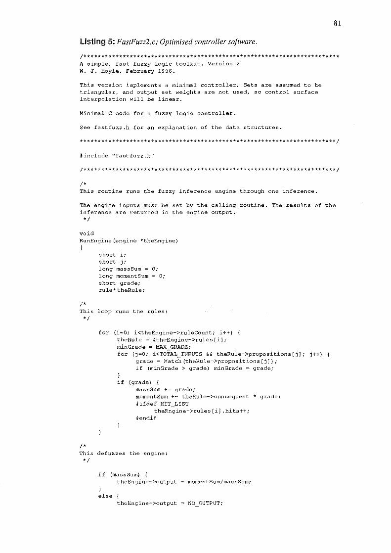
81
listing 5: FastFuzz2.c; Optimised controller software.
/************************************************************************ A simple, fast fuzzy logic toolkit. Version 2 W. J. Hoyle, February 1996.
This version implements a minimal controller; Sets are assumed to be triangular, and output set weights are not used, so control surface interpolation will be linear.
Minimal C code for a fuzzy logic controller.
See fastfuzz.h for an explanation of the data structures.
************************************************************************/
#inc1ude "fastfuzz.h"
/***********************************************************************/
/* This routine runs the fuzzy inference engine through one inference.
The engine inputs must be set by the calling routine. The results of the inference are returned in the engine output. */
void RunEngine(engine *theEngine) {
/*
short i; short j; long massSum 0; long momentSum = 0; short grade; rule * theRu1e;
This loop runs the rules: */
/*
for (i=O; i<theEngine->ru1eCount; i++) theRu1e = &theEngine->ru1es[i]; minGrade = MAX_GRADE: for (j=O; i<TOTAL_INPUTS && theRu1e->propositions[j); j++) (
grade = Match(theRule->propositions[j); if (minGrade > grade) min Grade grade;
if (grade) massSum += grade; momentSum += theRule->consequent * grade; Hfdef
theEngine->ru1es[i] .hits++; #endif
This defuzzes the engine: */
if (massSum) { theEngine->output
else
momentSum/massSum;
theEngine->output = NO_OUTPUT;

82
/***********************************************************************/
short Match(proposition* p) {
short setO; short setl: short set2: short input; long grade
if (p) {
/*
/* position /* position /* position
MAX_GRADE;
of of of
left set point (grade 0) * / second set point (grade MAX_GRADE) */ right set point (grade = O) */
Find the membership grade of the input in the antecedent set. Points 0 and 2 are assumed to have a grade of 0, point 1 is assumed to have a grade of MAX GRADE. */
/*
setO setl set2 input
p->antecedent[Oli p->antecedent[l]; p->antecedent[2]i
*(p->input}i
first check to see if the input is outside the set: */
if (input >= set2 I I input <= setO) { return (input setl)? MAX GRADE 0;
/* do an intersection with the left diagonal of the set if the input is left of the second set point: */
else
1*
if (input < setl) { grade *= (input setO); grade /= (set1 setO):
otherwise do an intersection with the right diagonal of the set: *1
else grade *= (input - set1); grade (long) MAX GRADE - grade / (set2 - set1);
return grade;
listing 6: Chromo.h; Public inteifaces for a chromosome class
/* chromo.h, Chromosome object for Dawkins vl.O: Genetic algorithm software for optimising stuff. W. J. Hoyle, Feb 1994.
*/

#include <fstream.h> #include <limits.h>
83
/************************************************************************ * A Chromosome's bit string is stored as an array of "word".
* * The following definitions are for portability. "word" should be * some native, unsigned int type that gives good speed on your machine. * WORD BIT then needs to be defined as the number of bits in the "word" * type.
* * The define "WORD" gives the array index of the word where the bit at * position "pos" is stored. Bit numbering in this implementation is * done according to the BigEndian convention (ie. MSB is at position 0).
* * The define "BASE_MASK" gives a mask of the base-most n bits in a word; * by base-most I mean lowest in memory (that is, the MS n bits on a * BigEndian machine, or the LS n bits on a LittleEndian machine). */
typedef #define #define
unsigned WORD BIT BIT (pos)
int word: (sizeof (word)*CHAR BIT) (~(~(word)O»l) » (pos)%WORD_BIT)
#ifdef BIG END IAN
#else
#define WORD (pos) #define BASE_MASK(n)
#define WORD (pos) #define BASE_MASK(n)
hndif
( (pos) /WORD_BIT) (~(word)O « WORD_BIT-(n»
«wordCount-l) - (pos)/WORD_BIT) (~(word)O » WORD_BIT-(n»
/************************************************************************ Chromosome class. This is the basic working object for managing bitstring storage and manipulation. */
class Population;
class Chromosome (
friend class Population:
Chromosome() {status = allocationError;
void ChromosomeInit(int theLength): void Copy (const Chromosome &it):
inline void Randomise(); void Mutate (double frequency); // crossOVer:
NULL;}
const Chromosome operator & (const Chromosome &mate) const:
unsigned int length: unsigned int wordCount; word * unsigned int marker; int status;
public:
enum
J ;
good, allocationError
inline Chromosome(unsigned int len) (ChromosomeInit(len);} inline Chromosome(const Chromosome &it);

inline Chromosome &operator (const Chromosome &it);
double fitness;
virtual -Chromosome() {delete[) string;}
int Status() const {return status;} int Good() const {return (status good);} inline void SetMarker(unsigned int point); inline word GetBit(unsigned int pos) const; inline void SetBit(word state, unsigned int pos); inline void ToggleBit(unsigned int pos); word CastToWord()
(return string[WORD(length») »WORD_BIT - length;) void UnGray(); Chromosome &operator »(Chromosome &dest): int operator =~(Chromosome& it);
84
friend ostream &operator «(ostream &out, const Chromosome &it); friend fstream &operator »(fstream &in, Chromosome &it):
} ;
1***************************************************** ******************* * Sets the current bit marker for a chromosome. Legal values are 0 to * length-I. *1
inline void Chromosome::SetMarker (unsigned int point)
marker ~ (point >= length) ? length-I : point;
1***************************************************** ******************* * To randomise a Chromosome's bits: *1
inline void Chromosome: :Randomise ()
Mutate(O.5);
1***************************************************** ******************* * Assignment ... *1
inline Chromosome &Chromosome::operator = (const Chromosome &it)
if (this != &it) II beware of *this *this. if (it.length > length)
delete string; II reallocate if we don't have enough space. string new word[it.wordCount);
Copy (it);
return *this;
1***************************************************** ******************* * Initialisation ••• *1
inline Chromosome::Chromosome(const Chromosome &it)
string = new word[it.wordCount]; Copy (it);

listing 6: Chromo.cpp; routines/or a C++ chromosome class
/* chromo.cpp, Chromosome object methods for Dawkins v1.0: Genetic algorithm software for optimising stuff. W. J. Hoyle, Feb 1994.
*/
#include <float.h> #include <iostream.h> #include "chromo.h" #include "utilities.h"
#define #define
CHROMOSOME HDR "Bit:" FITNESS "Fit:"
85
/************************************************************************ * These are the constructors for the Chromosome type, The null constructor * and initialiser function are provided to facillitate dynamic allocation.
* * This is the basic working object for managing bitstring storage and * manipulation.
* * The methods and operators are explained in the commented code. */
void Chromosome::ChromosomeInit (int theLength)
if (theLength > O) length = theLength: wordCount = length/WORD_BIT: if (length%WORD_BIT != 0) {
wordCount++;
string = new word[wordCount]; if (string) {
status = good; marker = 0; return;
status allocationError;
// success
/************************************************************************ * Bit fetch. Returns the bit at position pos. */
inline word Chromosome::GetBit (unsigned int pos) const
int theWord = WORD(pos}: word theBit = BIT(pos};
return string [theWord] & theBit;
/************************************************************************ * Sets the bit at position pos to (theBit) ? 1:0. */
inline void Chromosome::SetBit (word state, un
int theWord = WORD(pos); word theBit = BIT(pos};
int pos)

86
state? (string [theWord] 1= theBit) (string [theWord) &= ~theBit);
1***************************************************** ******************* * To toggle a bit. *1
inline void Chromosome::ToggleBit (unsigned int pos)
int theWord WORD(poS)i word theBit = BIT(pos);
string [theWord) A= theBit;
1************************************************************************ * This operator reads bits from *this, starting from bit this->marker, and * writes them to the dest Chromosome, from bit 0, until either we * run out of bits or fill up dest. See the file test.cpp for an example of * its use. *1
Chromosome &Chromosome::operator »(Chromosome &dest)
for (dest.marker=Oi dest.marker<dest.length && marker<length;) dest.SetBit(GetBit(marker++), dest.marker++);
return *this;
1***************************************************** ******************* * To mutate a Chromosome's bits with probability "frequency": *1
void Chromosome::Mutate (double frequency)
for (int i=O; i<length: i++) if (RandomOtol () < freque,ncy)
ToggleBit (i) ;
1************************************************************************ * The crossover operator: * This method fills a Chromosome with bits from two "parents" by crossing * their bit strings at some random point. It should only be used in * populations with constant length Chromosomes. *1
const Chromosome Chromosome::operator & (const Chromosome &mate) const
Chromosome kid(length); II assume length == this->length
1* generate a random cut point in the range 1 to length-I:
*1 int cut = RandomOtol()*(length-l) + 1;
1* copy some bits from the calling parent:
*1 for (int i=O: i<cut/WORD_BIT: i++)
kid.string[i] string [i 1 ;

87
1* copy some bits from both parents to make up the word where the cut point occurs:
*1
1*
word baseBits kid.string[i]
BASE_MASK(cut%WORD_BIT); string[i]&baseBits I mate.string[i]&-baseBits;
copy some bits from the mate: *1
while (++i < mate.wordCount) kid.string[i] = mate.string[il;
return kid;
1***************************************************** ******************* * == operator (for debugging) . *1
int Chromosome::operator (Chromosome& it) {
if (length != it. length) return 0;
for tint i=O; i<length; i++) if (GetBit(i) != it.GetBit(i») return 0;
return 1;
1***************************************************** ******************* * This method dumps a text representation of a Chromosome to the * specified ostream. *1
ostream &operator «(ostream &out, const Chromosome &it)
out « CHROMOSOME_HDR; for (int pos=O; pos<it.length; pos++) (
out « (it.GetBit(pos) ? 'I': '0');
out « n\n" « FITNESS_HDR; int Oldprecision = out.precision out « it.fitness; out.precision(Oldprecision);
return out;
1***************************************************** ******************* * Restore a Chromosome from a file: *1
fstream &operator »(fstream &in, Chromosome &it)
char bit;
in »WaitFor(CHROMOSOME_HDR); if (in) {
II wait for the header •••
for (int pos=O; pos<it.length; pos++) { in » bit; it.SetBit(bit-'O', pos);
in » WaitFor(FITNESS_HDR) » it. fitness;

88
return in;
1***************************************************** ******************* * Copier ••• for assignment and initialisation. *1
void Chromosome::Copy (const Chromosome &it)
1
length = it. length; wordCount = it.wordCount; marker = it. marker; fitness = it.fitness;
if (string) { status good;
else
for (int i=O; i<wordCount; i++) string[ij = it.string[i];
status allocationError;
*************************************************************************** * This method changes a Chromosome from Gray coding to binary coding. * It is intended that the large Chromosomes in the population are read, * in sections, into smaller ones for decoding by your fitness * function. See the test.cpp file for examples. Gray coding can be * helpful in genetic algorithms because it spreads the selection pressure * on an allele more evenly over its component bits. For example: if * the optimum value for a gene (say 8 bits out of the Chromosome) is * 128, and our fitness function simply returns the error, there will be * a strong selection pressure on the MSB, and minimal pressure on the low * order bits but the final accuracy relies on the algorithm selecting * the low order bits correctly. Gray coding encourages more accurate * results, and prevents premature convergence. *1
void Chromosome::UnGray()
for (int i = 0 ; i < length-1; i++) if (GetBit(i» ToggleBit(i+1);
Listing 7: Pop.h; public inteifacesfor a C++ popUlation class
1* pop.h, Population object for Dawkins v1.0: Genetic algorithm software for optimising stuff. W. J. Hoyle, Feb 1994.
*1
#include <fstream.h>
1***************************************************** ******************* * Your fitness function must be of this type. It should evaluate the fitness * of the Chromosome passed to it and save the value in the Chromosome's * fitness variable (a double). The fitness variables can have values anywhere * in the range that double covers. This code works to maximise "fitness" * if it is more convenient to work to minimum "fitness" just change *1

89
typedef void fitnessFunction (Chromosome &); typedef fitnessFunction *fitnessFunctionPtr;
I ***************************************************************************
* Population Type. This class holds the population of Chromosomes, and * provides functions for selecting and combining them to implement the GA. * See the file pop.cpp for a full explanation of the use of this type. *1
class Population { unsigned int size; unsigned int length; int generation: double mutationRate: unsigned int gap; double
lithe number of Chromosomes lithe length of Chromosomes lithe number of this generation Ilyep. lithe generation gap.
double totalFitness; int status;
Iisimple Population fitness profiler Iisum of scaled fitness values. Iiallocation status.
Chromosome* currentPop; Chromosome* nextPop; double* rouletteWheel; Chromosome** rank;
Ilpointer to the current array Ilwhere to build the next one. Ilholds scaled fitness values. Ilholds a ranked list of pointers to
Chromosomes.
void Populationlnit(); Population &operator =(const Population&); Population (const Population&); const Chromosome &Select() const; void Sort(); inline void Swap(int a, int b); void CrapSort () ; void Breed () ; void Mutate () ; void Evaluate(); void Rank () :
fitnessFunctionPtr FitnessFunction:
pUblic:
enum
} ;
good, allocationError, zeroFitness
Population (
) ;
unsigned int size, unsigned int length, fitnessFunctionPtr theFF, double mutation 0.001, double theGap 0.02, double greed = 1.0
II can't assign II or copy
Population (fstream &in, fitnessFunctionPtr theFF); virtual -Population():
int Status() const {return status;} int Good() const {return (status good):} void TheNextGeneration(); void Stats(ostream &out) const; double AverageFitness() const; double MaxFitness() const (return BestChromosome() .fitness;} Chromosome &BestChromosome() const {return *rank[O];}

90
friend ostream &operator «(ostream &out, const Population &it)i } :
listing 8: Pop.cpp,· a c++ population class
/* pop.cpp, Population methods for Dawkins v1.0: Genetic algorithm software for optimising stuff. W. J. Hoyle, Feb 1994. */
#include <math.h> #include <iostream.h> #include "Dawkins.h"
#define file:" #define #define #define #define #define #define #define
FILE HDR
SIZE HDR LENGTH HDR MUTATION HDR GAP HDR GREED HDR GENERATION HDR FILE END
"Dawkins.cpp GA library, v1.0. Population
"Population size:" "Chromosome length:" "Probability of bit mutation:" "Generation gap:" "Greedy selection exponent:" "Generation:" "End of file."
#ifdef HAVE CONSTANT FF ltdefine EVALUATE FROM gap
#else #define
#endif EVALUATE FROM o
/************************************************************************ The constructor for the Population class: This is the heart of the library. To work the algorithm, first create a popUlation object by passing the following parameters to its constructor:
int theSize: the number of Chromosome objects in the population. The optimum depends mainly on Chromosome size -- a population of 100 is plenty for Chromosomes of 30-40 bits in length, but after 40 bits optimal popUlation size grows rapidly (at least in theory), and time constraints tend to govern the choice. See Goldberg, D.E. "Sizing Populations for Serial and Parallel Genetic Algorithms", the Proceedings of the Third International Conference on Genetic Algorithms, 1989.
int theLength: the number of bits in each Chromosome in the popUlation. Try not to go overboard on accuarcy, the algorithm will take forever to reach a solution if the Chromosomes are too long. Consider using the GA to find the correct global maximum/minimum and then conducting a finer search in that area.
fitnessFunctionPtr theFF: a pointer to your fitness function. This is the function that you provide to rank the Chromosomes in the population. Your function will be passed a reference to a Chromosome, it should store some index of performance in Chromosome. fitness. The performance index can have a value anywhere in the range that type "double" covers. This code in this library works to maximise "fitness" if it is more convenient to work to minimum "fitness" just change sign.
double mutation: the likleyhood of a particular bit in the population undergoing mutation. This is a secondary search operator: it is included to guard against the loss of information from the bit pool during the later stages of the run, when the alleles assosiated with fitter Chormosomes begin to dominate population. To put it another way, if one particular bit (say position one) of every Chromosome in the population holds an identical value (say 1) then the crossover operator

91
cannot reintroduce the lost information (ie no Chromosome can gain a o in bit one). The mutation operator has a default value of 0.001. Values above 0.05 tend to do more harm than good, by giving the algorithm too much of a random search characteristic.
double theGap: A coefficient for the generation gap. Legal values are 0-1. This specifies the fraction of the population that is copied to the next without alteration. Doing this ensures that the best Chromosomes are never lost. It also gives them a better chance of being chosen for crossover (that is, it implements a "greedy" selection scheme), because they will take part in subsequent selection rounds. The default value for this variable is 0.02. If this code has compiled with the switch HAVE_CONSTANT-YF fdefined, it will not pass your fitness function the Chromosomes that have been copied directly, and will therefore run somewhat faster.
double greediness: exponent for a simple greedy selection scheme. This uses dynamic fitness scaling over a scaling window of 1 -- after
one generation of Chromosomes has been evaluated by your fitness function their fitness values are scaled into the range 0 to 1. This approach was taken because it allows your fitness function to return some arbitary index of performance (some schemes require the index of fitness to be positive and in some range), and because emperical evidence suggests that a scaling window of 1 generation gives better performance (see Greffenstette, J.J. "Optimisation of Control Parameters for Genetic Algorithms", IEEE Transactions on Systems, Man, and Cybernetics, 16, Number 1, 1986). Greedy selection involves giving fitter organisms a better chance of reproduction than their index of fitness would indicate
with the objective of faster convergence. This can be useful, but if abused will lead to premature convergence (ie the loss of useful alleles from the population see the discussion on mutation, above). This library implements a simple greedy selection scheme by raising the scaled fitness of every Chromosome to a power (the greed exponent) • This depresses the fitness values of the lesser Chromosomes, but leaves the fittest (which always has a fitness of 1 after scaling) untouched. The default greediness of 1.0 has no effect (ie no greedy selection), 2.0 is mild, and 5.0 is heavy. Values from 0.0 to 1.0 have the opposite effect, (sort of egalitarian ... ) and may have some use in preventing premature convergence in cases where selection pressure is already profound.
*1
Population::Population( unsigned int theSize, unsigned int theLength, fitnessFunctionPtr theFF, double mutation, double theGap, double greediness
size (theSize) , length(theLength}, FitnessFunction(theFF}, mutationRate(mutation}, gap (theGap) , greed(greediness}, generation (0)
PopulationInit(); if (Good ()) {
gap theGap*size; if (gap >= size) gap = size-1; for (int i=O; i<size; i++) {
currentPop[il.Randomise();
Evaluate () i
Rank () i
II what have we got? II sort them out.

92
1***************************************************** ******************* * Construct a population from a file: *1
Population::Population(fstream &in, fitnessFunctionPtr theFF) FitnessFunction(theFF)
in.seekp(O); in » WaitFor(FILE_HDR); if (in) {
in » WaitFor(SIZE_HDR) » size; if (in) {
status
in » WaitFor(LENGTH_HDR) » length; if (in) {
in » WaitFor(MUTATION_HDR) » mutationRate; if (in) {
in » WaitFor(GAP_HDR) » gap; if (in) {
allocationError;
in » WaitFor(GREED_HDR) » greed; if (in) {
in » WaitFor(GENERATION_HDR) » generation; if (in) {
Populationlnit(); if (Good () {
for (int i=O; i<size && (in); i++) {
in » currentPop[ij;
in »WaitFor(FILE_END); if (in) {
Rank () ; return; II success
1***************************************************** ******************* * Memory allocation for the Population class: *1
void Population::Populationlnit()
status good; nextPop NULL; rouletteWheel rank = NULL;
I I optimism ... II in case we fail, and have to call the dtor.
NULL; II ditto. II double ditto.
currentPop = new Chromosome[sizel; if (currentPop) {
nextPop = new Chromosome[size); if (nextPop) {
for (int i=O; i<size; i++) currentPop[i] .Chromosomelnit(length); if (!currentPop[i) .Good(» {

status break:
allocationError:
nextPop[ij.ChromosomeInit(length): if (!nextPop[i].Good(» {
if (Good()}
status = allocationError: break:
rouletteWheel = new double[size]: if (rouletteWheel) {
rank = new Chromosome*[size]: if (rank) {
return; II success at last ...
status allocationError;
93
1***************************************************** ******************* * Memory deallocation for the Population class: *1
Population::-Population() {
delete[] currentPop; delete[J nextPop; delete[] rouletteWheel; delete[] rank;
1***************************************************** ******************* * This is where everything comes just allocate your population * ob , and apply this method to it until the answer looks good enough. *1
void Population::TheNextGeneration()
Breed(); Mutate(): Evaluate(); Rank();
1***************************************************** ******************* * This function calls your fitness fUnction for each Chromosome in the * population. *1
void Population::Evaluate()
1* Call the fitness function for every Chromosome in the Population. Unless the switch HAVE CONSTANT FF has beed #defined.
If a Chromosome has been copied directly (by the Breed() method, in accordance with the generation gap coefficient) - the fitness func-tion remains constant from generation to generation - then its fitness will already be correct (that is, it will have been evaluated correctly during a previous . Define the switch HAVE_CONSTANT_FF (to save time by avioding needless re-evaluation) if this is the case. If this is the first we have to evaluate everything anyway.
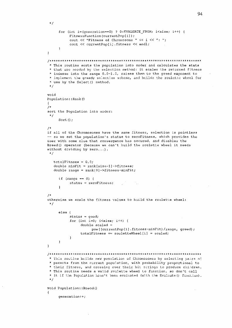
*/
for (int i=(generation==O) ? O:EVALUATE_FROM; i<size; i++) FitnessFunction(currentPop[ij); cout « "Fitness of Chromosome II « i « ": "; cout « currentPop[ij .fitness « endl;
94
/************************************************************************ * This routine sorts the population into order and calculates the stats * that are needed by the selection method: it scales the returned fitness * indexes into the range 0.0-1.0, raises them to the greed exponent to * implement the greedy selection scheme, and builds the roulette wheel for * use by the Select() method. */
void Population::Rank() {
/* sort the Population into order: */
Sort () i
/* if all of the Chromosomes have the same fitness, selection is pointless
so we set the population's status to zeroFitness, which provides the user with some clue that convergence has occured, and disables the Breed() operator (because we can't build the roulette wheel it needs without dividing by zero ... ). */
/*
totalFitness = 0.0; double minFit = rank[size-l]->fitness; double range = rank[O]->fitness-minFit;
if (range == 0) { status zeroFitness;
otherwise we scale the fitness values to build the roulette wheel: */
else status good; for (int i=O; i<size; i++) (
double scaled =
pow«currentPop[i] .fitness-minFit)/range, greed); totalFitness += rouletteWheel[i] = scaled;
/************************************************************************ * This routine builds new population of Chromosomes by select pairs of * parents from the current population, with probability proportional to * their fitness, and crossing over their bit strings to produce children. * This routine needs a valid roulette wheel to function, so don't call * it if the Population hasn I t been evaluated (with the Evaluate () function). */
void Population::Breed()
generation++;

1* first, check to see that the population has some range of fitness:
*1 if (status != zeroFitness) {
1* transfer the best Chromosomes without alteration:
*1
1*
for (int i=O; i<gap; i++) { nextPop[i] = *rank[i];
make some kids: *1
1*
while (i<size) ( nextPop[i++] Select() & Select(); II crossover.
swap the new population and current population: *1
Chromosome *temp = currentPop; currentPop = nextPoPi nextPop = tempi
95
1***************************************************** ******************* * This routine applies the mutation operator to every Chromosome in the * population except those preserved by the generation gap constant. *1
void Population::Mutate()
for (int i=gapi i<size; i++) { currentPop[i] .Mutate(mutationRate);
1***************************************************** ******************* * This selects a Chromosome from the population with a probability * proportional to its scaled fitness. *1
const Chromosome &Population::Select() const
1* spin the wheel ... *1
1*
double spot = RandomOtol() * totalFitness; double currentSpot = 0.0; int i=O;
find where it landed ... *1
while «currentSpot += rouletteWheel[i]) < spot) i++;
1* return the lucky punter:
*1 return currentPop[i];
1***************************************************** ******************* * A simple reporting function:

*1
void Population::Stats(ostream &out) const
out « "generation: " « generation « "\n"; out« "average:"« AverageFitness()« "\n"; out « "best: .. « "\n" « BestChromosome () « endl;
96
1***************************************************** ******************* * This function returns the population's average (unsealed) fitness: *1
double Population::AverageFitness() const {
double total 0; for (int i=O; i<size; i++) {
total += currentPop[i] .fitness;
return total/size;
1***************************************************** ******************* * Dump a text representation of a Population to an ostream: *1
ostream &operator «(ostream &out, const Population &it)
out « FILE HDR « "\n\n"; out « SIZE HDR « it. size « "\n"; out « LENGTH HDR « it.length « "\n"; out « MUTATION HDR « it.mutationRate « "\n"; out « GAP HDR « it.gap « "\n"; out « GREED HDR « it. « "\n\n"; out « GENERATION HDR « it.generation « "\n\n"; for (int i=O; i<it. size && out; i++) {
out « *it.rank[i] « "\n";
out « "\n" « FILE END « end~;
return out;
1***************************************************** ******************* * CrapSort: * This sorts the current population into * swapping pointers (held in the array "rank") * Population. *1
void Population::Sort()
order (of fitness) by to the individuals in the
for (int i=O; i<size; i++) { rank[il = currentPop+i; II initialise pointers.
CrapSort () ;
inline void Population::Swap(int at int b) {
void
Chromosome* temp = rank[a]; rank[a] rank[bJ; rank[b] = temp;

Population::CrapSort() {
for (int i=O; i<size-1; i++) { for (int j=i+1; j<size; ) {
if (rank[ij->fitness < rank[jj->fitness) Swap(i,j):
Listing 9: utilities.h; public interfaces for some SGA utility functions
1*
97
utilities.h, miscellaneous declarations and definitions for Dawkins v1.0: Genetic algorithm software for optimising stuff. W. J. Hoyle, Feb 1994.
*1
finclude <iomanip.h>
1***************************************************** ******************* * This should return a double in the range 0.0 to 1.0. * Patch in your favourite random number generator here .••
* * I use the fdefine ULTRA to patch in a random number generator (see * below, and Dawkinslnit: :Dawkinslnit(), in "utilities.cppn. Either lundef * ULTRA, in which case the standard C RNG will be used, or patch in your own * RNG. *1
Hfdef ULTRA
#else
4finclude "Ultra.h" #define MY_RANDOM
#include <stdlib.h>
--------- ()
#define MY RANDOM ((double) rand()/RAND_MAX) #endif
inline double RandomOto1() ( return MY_RANDOM:
1***************************************************** ******************* * The waitfor ..• operator. This waits for the string in the * specified fstream. *1
lMANIP<char *> WaitFor(char *theString);
Listing 10: utilities.cpp; some utilitiesfunctionsfor a SGA
1* utilities.cpp, Miscellaneous functions for Dawkins v1.0: Genetic algotithm software for optimising stuff. W. J. Hoyle, Feb 1994.
*1
#include <fstream.h> #include <time.h> #include "utilities.h"
1***************************************************** ******************* * This manipulator waits for the delimiting "theString" in an * istream and then returns. The stream will be EOF if the operation fails. *1
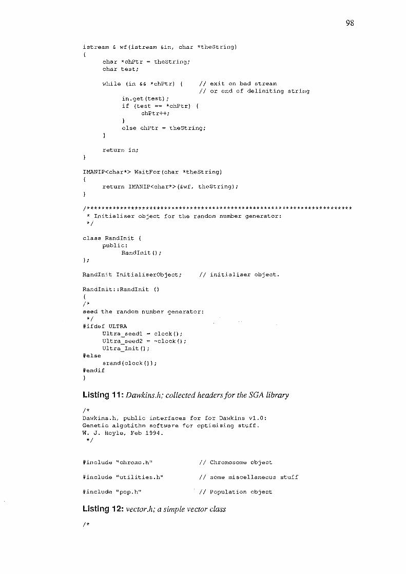
istream & wf(istream &in, char *theString)
char *chptr = theString; char test;
while (in && *chptr)
in.get(test); if (test == *chPtr)
chPtr++;
II exit on bad stream II or end of delimiting string
else chPtr = theStringi
return in;
lMANIP<char*> WaitFor(char *thestring) {
return lMANIP<char*> (&wf, theString);
98
1***************************************************** ******************* * Initialiser object for the random number generator: *1
class Randlnit { public:
Randlnit () ; } ;
Randlnit InitialiserObject;
Randlnit::Randlnit ()
1*
II initialiser object.
seed the random number generator: *1
/Hfdef ULTRA
ltelse
Ultra seedl Ultra seed2 Ultra_Init ();
clock (); ~clock () ;
srand(clock (); ltendif }
listing 11: Dawkins.h; collected headers for the SGA library
1* Dawkins.h, public interfaces for for Dawkins vl.O: Genetic algotithm software for optimising stuff. W. J. Hoyle, Feb 1994.
*1
ltinclude "chromo.h" II Chromosome object
ltinclude "utilities.h" II some miscellaneous stuff
ltinclude "pop.h" II Population object
listing 12: vector.h; a simple vector class
1*

A vector class: */
*ifndef VECTOR HEADER *define VECTOR HEADER
*include <math.h>
class vector ( unsigned int size; double *numbers;
inline void copy(const vector &it);
public: vector() (numbers = 0;)
99
vector(unsigned int size) : size (size) (numbers inline vector(const vector &it);
new double[size]:}
-vector() {delete[] numbers:}
inline vector *vectorInit(const unsigned int size); inline unsigned int Size() {return size;} inline void abs(): inline void pow (double exponent); inline double minI) const: inline double maxI) const; friend inline vector abs(const vector &it): friend inline vector pow(const vector &it, double exponent); inline vector &operator =(const vector &it); inline double &operator [] (const uns int i) (return numbers[i];) inline double operator (I (canst unsigned int i) canst (return numbers[il;) inline vector &operator +=(const vector&it); inline vector &operator -=(const vector&it); inline vector &operator *=(const vector&it): inline vector &operator /=(const vector&it);
inline vector operator + (const vector&it) ; inline vector operator (const vector&it) ; inline vector operator * (const v'ector&it) ; inline vector operator /(const vector&it) ;
inline vector &operator +=(const double scalar); inline vector &operator -=(const double scalar): inline vector &operator *=(const double scalar) : inline vector &operator /=(const double scalar);
inline vector operator + (const double scalar) ; inline vector operator -(const double scalar); inline vector operator * (const double scalar): inline vector operator /(const double scalar):
friend inline vector operator + (const double scalar, friend inline vector operator -(const double scalar, friend inline vector operator * (const double scalar, friend inline vector operator /(const double scalar,
} ;
inline void vector: :copy(const vector &it) {
size = it. size; for (unsigned int
numbers [i) i=O: i<size; i++) it.numbers[il:
inline vector::vector(const vector &it)
canst vector &it) : canst vector &i t) ; const vector &i t) ; const vector &it) :

numbers = new double[it.sizel; copy(it);
inline vector *vector::vectorlnit(const unsigned int size)
numbers = new double[sizel; vector::size = size;
return (vector *) numbers;
inline vector &vector::operator (const vector &it)
if (it. size ! = size) { delete numbers; numbers = new double[it.sizel;
copy (it); return *this;
inline void vector::abs()
for (unsigned int i=O; i<size; i++) { if (numbers[il < 0) (
numbers[ij O-numbers[il;
inline vector abs(vector &it)
vector v = it; v.abs(): return v;
inline void vector: :pow(double exponent)
for (unsigned int i=O; i<size; i++) numbers[il : :pow(numbers[il, exponent);
inline vector pow (vector &it, double exponent)
vector v = it; v.pow(exponent); return v;
inline double vector: :min() const
double min numbers[O); for (unsigned int i=l; i<size; i++) {
if (numbers[il < min) { min = numbers[il;
return min;
inline double vector::max() const
double max numbers [OJ; for (unsigned int i=l; i<size; i++) {
if (numbers[il > max) { max = numbers[il:
100

return max;
inline vector &vector::operator +=(const vector &it)
for (unsigned int i=O; i<size; i++) numbers [i) += it.numbers[i);
return *this;
inline vector &vector::operator -=(const vector &it)
for (unsigned int i=O; i<size; i++) numbers [i) -= it.numbers[i);
return *this;
inline vector &vector::operator *=(const vector &it)
for (unsigned int i=O; i<sizei i++) numbers [i) *= it.numbers[i);
return *this;
inline vector &vector::operator /=(const vector &it)
for (unsigned int i=O; i<size; i++) numbers [i) /= it.numbers[ili
return *this;
inline vector vector: :operator +(const vector &it)
vector v *this; v += it; retprn v;
inline vector vector::operator -(const vector &it)
vector v = *this; v it; return Vi
inline vector vector: :operator *(const vector &it)
vector v = *this; v *= it; return v;
inline vector vector::operator /(const vector &it)
vector v *this; v /= it; return v;
inline vector operator + (const double scalar, const vector &it)
vector v = it; for (unsigned int i=O; i<v.size; i++)
v.numbers[i) = scalar/v.numbers[i]:
return v;
inline vector operator -(const double scalar, const vector &it)
101

vector v = it; for (unsigned int i=O; i<v.size; i++)
v.numbers[i] = scalar-v.numbers[il;
return v;
inline vector operator * (const double scalar, const vector &it)
vector v = it; for (unsigned int i=O; i<v.size; i++)
v.numbers[i] = scalar*v.numbers[il;
return v;
inline vector operator 1 (const double scalar, const vector &it)
vector v = it; for (unsigned int
v.numbers[i]
return v;
i=O; i<v.size; i++) scalar/v.numbers[il;
inline vector &vector::operator +=(const double scalar)
for (unsigned int i=O; i<size; i++) numbers[iJ += scalar;
return *this;
inline vector &vector::operator -=(const double scalar)
for (unsigned int i=O; i<size; i++) numbers[iJ scalar;
return *this:
inline vector &vector::operator *=(const double scalar)
for (unsigned int i=O; i<size; i++) numbers[i] *= scalar;
return *this;
inline vector &vector::operator I=(const double scalar)
for (unsigned int i=O; i<size; i++) numbers[iJ 1= scalar;
return *this;
inline vector vector: :operator +(const double scalar)
vector v *this; v += scalar; return v;
inline vector vector: :operator (const double scalar)
vector v *this; v -= scalar; return Vj
102

inline vector vector::operator * (const double scalar) (
vector v = *this; v *= scalari return v;
inline vector vector::operator I(const double scalar)
vec.tor v = *this; v 1= scalar; return Vi
#endif
listi ng 13: sint.h; an abstract base class/or a simple integrator
1* Simple integrator, abstract base class:
*1
#ifndef SINT HEADER #define SINT HEADER
#include "vector.hl!
typedef vector &dFunc(double t, const vector &state, vector& stateD); typedef dFunc *dFuncPtr;
class SIntegrator ( protected:
double h, hmax; double t; dFuncPtr dfn; vector state; vector stateD;
II step size II time II pointer to your derivative function II the state vector II the state derivative
public:
} ;
SIntegrator(vector &init, dFuncPtr dfn, double t, double h); virtual ~SIntegrator() ()
virtual void Step() = 0; virtual void StepTo(const double endT)i double Time() const {return til vector State() const {return state:} double operator () (const unsigned int i) const (return state(i):}
#endif
listing 13: sint.cpp,· utilities/or the abstract base class 0/ a simple integrator
1* Base class utilities for a simple
*1
#include "sint.h"
103
SIntegrator::Slntegrator(vector &init, dFuncPtr dfn, double t, double h): state (init) , stateD(init.Size(», dfn (dfn), t (t),
h(h) , hmax(h)
{}
void SIntegrator::StepTo(const double endT)

h '= hmax: while (t<endT)
if (t+h > endT) h = endT-t:
Step () ;
Listing 13: rk4 .h; public interfaces for a Runge-Kutta (order 4) integrator
1* Public interfaces for a Runge-Kutta (order 4) de solver:
*1
'include "sint.h"
class rk4 : public SIntegrator vector kl, k2, k3, k4i
pUblic:
II working variables
rk4(vector &init, dFuncptr dfn, double t, double h): virtual -rk4() I}
virtual void Step(); } ;
Listing 14: rk4.cpp; a Runge-Kutta (order 4) integrator
1* Runge-Kutta (order 4) de solver:
*1
#include "rk4.h"
rk4::rk4(vector &init, dFuncPtr dfn, double t, double h):
{}
SIntegrator(init, dfn, t, h), kl (init.Size (»,
k2 (init. Size (»,
k3 (init. Size (»,
k4 (init. Size (»
void rk4:: Step ()
1* pretty: kl h * dfn(t, state, stateD) : k2 h * dfn(t + h/2, state + kl/2, stateD): k3 h * dfn(t + h/2, state + k2/2, stateD) ; k4 h * dfn(t + h, state + k3, stateD) ;
state += (kl + 2*k2 + 2*k3 + k4)/6; t += h; *1
II ugly but generally faster:
kl dfn(t, state, stateD) ; kl *= h/2; k2 dfn(t + h/2, state + kl, stateD); k2 *= h/2; k3 dfn(t + h/2, state + k2, stateD) ; k3 *""- h; k4 = dfn(t + h, state + k3, stateD); k4 *= hi kl *= 2;
104

k2 *'" 4; k3 *'" 2; k1 +'" k2; k1 += k3; k1 + .. k4; k1 /'" 6; state +'" k1;
t += hI
listing 15: main.cpp; example codefor the SGA
/* test.cpp, testbed for for Dawkins v1.0: Genetic algotithm software for optimising stuff. W. J. Hoyle, Feb 1994. */
#include #include #inc1ude #include #include #include #include
#define #define
#define
<iostream.h> <stdlib.h> <math.h> "Dawkins.h" "SimFan.h" IMatArray" "controller.h"
DEG TO RAD ROUND_SHORT (x)
FILE_NAME "Fan.pop"
(2.0*3.141592653589793/360.0) «short) «x)+0.5»
OUTPUT PRECISION 6 SIZE 100
105
#define #define #define #define #define #define
LENGTH MUTATE
GAP GREED
OUTPUT_PRECISION*(TOTAL_RULES-PREDEFINED_RULES) 0.005 0.05 1.0
fitnessFunction MyFF; int InitPopulation(fstream& popFile); void BuildEngine(Chromosome &it); void WalkEngine(engine* theEngine, int input1, int input2, fstream& out); double Completeness (engine *e):
Population* pop;
void main ()
cout « "Testbed for Dawkins vI. 0 SGA ... \n" « endl;
fstream popFile(FILE_NAME);
if (InitPopulation(popFile»
int i;
unsigned short g;
cout « "How many generations? It;
cin » g;
fstream mon(IIMonitor", ios: :outlios: :applios: :translated);
for (i=O: i<g; i++) ( pop->TheNextGeneration();

pop->Stats(cout); cout « endl; mon « pop->BestChromosome () . fitness « ", \n";
cout « "Saving population to file " « FILE NAME « endl; popFile. close () ; popFile.open (FILE_NAME, ios::inlios::outlios::translatedlios::trunc); popFile « *pop;
BuildEngine(pop->BestChromosome(»;
#ifdef HIT LIST for (i=O; i<TOTAL_RULES; i++) {
controller.rules[i] .hits 0:
#endif
fstream graphFile5 ("5 deg Graph", ios::outlios::trunclios::translated); FanGraph(graphFile5, &controller, 5.0*DEG_TO_RAD); fstream graphFile20 ("20 deg Graph", ios::outlios::trunclios::translated); FanGraph(graphFile20, &controller, 20.0*DEG_TO_RAD); fstream graphFile45 ("45 deg Graph", ios::outlios::trunclios::translated): FanGraph(graphFile45, &controller, 45.0*DEG_TO_RAD);
#ifdef HIT LIST fstream hitFile ("Rule hits", ios:: out I ios: :trunc I ios: : translated) ; hitFile « setprecision(3) « showpoint « fixed; int totalHits = 0: for (i=O: i<TOTAL_RQLES; i++)
totalHits += controller.rules[il .hits;
for (i=O: i<TOTAL_RULES; i++) ( hitFile « setw(6);
106
hitFile « controller.rules[i] .hits/totalHits*100: hitFi1e « "%, ";
#endif
hitFile « controller.rules[i].hits; hitFile « " hits on rule" « i+1 « "\n";
fstream outFile ("Rule outputs", ios: lout I ios: :trunc I ios: :translated) ; outFile « setprecision(2) « showpoint « fixed: for (i=O; i<TOTAL_RULES; i++) (
outFile « setw(10); outFile « controller.rules[il .consequent*aOOO.O/MAX_GRADE; outFile « " Nm, "; outFile « controller. rules [i) . consequent; outFile « ", output from rule" « setw(3) « i+1 « endl;
controller. inputs [0] 10; controller. inputs [1] 0; controller. inputs [2] 10; RunEngine(&controller);
controller. inputs [1] = 0; II acceleration 0

else
fstream surfaceD ("surfaceO", ios: :outlios: :trunclios: :translated); WalkEngine(&controller, 0, 2, surfaceO); controller. inputs [1] = 127: fstream surfacel (" surface1", ios:: out I ios : : trunc I ios: : trans lated) :
WalkEngine (&controller, 0, 2, surface1); controller. inputs [1] 255; fstream surface2 ("surface2", ios::outlios::trunclios::translated); WalkEngine(&controller, 0, 2, surface2);
107
cout « "Error: couldn't initialise the population." « endl;
void MyFF(Chromosome &it) (
BuildEngine (it) ; it.fitness ~ -FanFitness(&controller, 5.0*DEG_TO_RAD); it.fitness FanFitness(&controller, 22.5*DEG_TO_RAD); it.fitness -= FanFitness(&controller, 45.0*DEG_TO_RAD);
void BuildEngine(Chromosome lit) (
int
static Chromosome bits(OUTPUT_PRECISION);
it .SetMarker (0);
for (int i=PREDEFINED_RULES; i<TOTAL_RULES; i++) { it » bits; bi ts . Un Gray () ; short raw = bits.CastToWord(); short scaled raw* (double) /lJAX_GRADE/ (pow (2, OUTPUT_PRECISION) -1)
127.5; controller.rules[iJ . consequent = scaled;
InitPopulation(fstream& popFile) {
popFile.seekp(O, ios::end); if (popFile.tellg(» (
else
pop = new Population(popFile, MyFF);
pop = new Population (SIZE, LENGTH, MyFF, MUTATE, GAP, GREED); if (pop) {
if (pop->Good(» { popFile « *pop;
if (!pop) return 0;
if (! pop->Good () ) return 0;

108
return 1;
1* This procedure creates a Mathematica Graphics3D file that describes the control surface of an It will only plot the complete parts of the rule base. *1
#define RESOLUTION 25 #define SURFACE STEP «double)MAX_GRADE/RESOLUTION)
void WalkEngine(engine* theEngine , int input1, int input2, fstream& out) (
out « "Graphics3D[{\n"i out « setprecision(3) « fixed; for (double x=O; ROUND_SHORT(x)<MAX_GRADE; x+=SURFACE_STEP) {
double x2 = x+SURFACE_STEP; for (double y=O; ROUND_SHORT(y)<MAX_GRADE; y+=SURFACE_STEP)
double y2 y+SURFACE_STEPi theEngine->inputs[inputl] = ROUND_SHORT(x); theEngine->inputs[input2] = ROUND_SHORT (y); if (Completeness (theEng ine) > 0.99) ( I I allow for errors.
RunEngine(theEngine); short zl = theEngine->outputi theEngine->inputs[input2] = ROUND_SHORT (y2);
if (Completeness (theEngine) > 0.99) RunEngine(theEngine)i short z2 = theEngine->outpUti theEngine->inputs[input1j = ROUND_SHORT(x2); if (Completeness (theEngine) > 0.99)
RunEngine(theEngine); short z3 theEngine->output; theEngine->inputs[input2J = ROUND_SHORT (y) ; if (Completeness (theEngine) >
RunEngine(theEngine); short z4 = theEngine->output; out « "Polygon[{"i out « "l" « x « II " « y « fI II « I , out « ul U « x « " " « y2 « fI II « , I
out « "( II « x2 « " " « y2 « " II « I ,
0.99) (
zl « ") I
22 « "),
23 « "),
II. , II. , II.
I
out « 11 {U « x2 « !! " « y « II TI « z4 « " ) ) ]" i I I
out « ",\nll;
out.seekp(-2, ios::cur); II get rid of out last comma and newline out « "\n}]" « endl;
1* This function calculates the completeness of the rule base for the current eng ine input s .
o is incomplete. (0, 1) is subcomplete. 1 is strict complete. > 1 is overcomplete.
There may be some rounding error.

*/
double Completeness(engine *e) (
double completeness 0; for (int r=O; r<e->ruleCount; r++) {
double ruleProduct (double) Match(e->rules[rj.propositions[O])/MAX_GRADE;
for (int p=l; p<TOTAL_INPUTS; p++) { ruleProduct *=
(double) Match(e->rules[rJ .propositions[pJ)/MAX_GRADE; }
completeness += ruleProduct;
return completeness;
109
listing 16: simfan.h; public interfaces for a variable pitch propeller simulation
/* SimFan .h Public interface for a propel lor simulation. */
#ifndef SIMFAN HEADER #define SIMFAN HEADER
#include <iostream.h> 'include "fastfuzz.h"
double FanFitness(engine* controller, double pI;
void FanGraph(ostream& out, engine* controller, double pI;
double* FanSimulation(engine* controller, double pI;
'endif
listing 17: simfan.cpp; a variable pitch propeller simulation
/* Fan Simulator: */
'include "rk4.h" #include "SimFan.h" 'include <math.h> #include <iostream.h>
0.25 #define 'define 'define #define
STEPS 320 TZERO 0.0 RAD TO_REV (1.0/(2.0*3.141592653589793»
dFunc myDFunc; double Accn(double n); short Sensor(double currentN);
double gTorque; double gPitch;
double FanFitness(engine* controller, double p) {
double* simArray = FanSimulation(controller, pI;

/* Our fitness is the error integral relative to a set point of 18 rad/s: */
double totalErr = 0.0;
int i=O; while(simArray[i]<17.5 && i<STEPS) i++; while (i<STEPS) {
totalErr += fabs«18.0-simArray[i])*STEP_SIZE); i++;
return totalErr;
void FanGraph(ostream& out, engine* controller, double p) {
double* simArray = FanSimu1ation(controller, p);
out « "ListPlot[{\n"; for (int i=O; i<STEPS; i++) {
out « simArray[i] « ",\n";
out.seekp(-2, ios::cur); out « "\n}, \n"; out « "{\n"; out « "PlotJoined->True,\n"; out « "AxesLabel->{\"seconds\", \"rad/s\"},\n"; out « "PlotRange->{{O,I! « STEPS « "},{O,20»,\n"; out « "Ticks->{ { {I, 0), {I! « STEPS « out « ") \n] \n";
double* FanSimulation(engine* controller, double p) {
static double simArray[STEPS]; vector initCond (1) ; short last Torque = 0; short next Torque 0; shortlastRawSpeed 0;
gPitch = p; gTorque = 0.0; initCond[O] = 0;
" ,
rk4 r(initCond, myDFunc, TZERO, STEP_SIZE);
for (int i=O; i<STEPS; i++) {
/* Set up controller inputs: */
/*
short rawSpeed = Sensor(r(O»; double speed = reO);
80}}, {O, 18)}\n";
First, scale the raw sensor reading into the range O-MAX_GRADE. 5867 sensor clicks/quarter second corresponds to a propellor speed of 18.0 rad/s , which is out set-point. Subtracting this from the raw
110
gives us a zero. In order to scale the zeroed reading so that the raw readings that represent the range 17.5-18.5 rad/s, we multiply by 4/5 and add 127. */

111
short n (rawSpeed - 5867)*4/5; II scale n into O-MAX GRADE n += MAX_GRADE/2;
if (n < 0) n 0; II clip if (n > MAX_GRADE) n = MAX_GRADE;
1* Now calculate the acceleration and scale it into 0-255, with 127 representing the set-point (that is, 0 acceleration). The maximum acceleration is about 0.75 rad/s/s. After scaling by 0.5 and adding 127, the range of accelerations represented is about -0.75 to +0.75 rad/s/s.
*1
1*
short a (rawSpeed - lastRawSpeed)/2; a +~ MAX_GRADE/2i
if (a < 0) a = 0; II clip if (a > MAX_GRADE) a = MAX_GRADE;
Put the inputs in the controller: *1
1*
controller->inputs[Oj controller->inputs[1j controller->inputs[2]
n; a; lastTorque;
Find the output: *1
1*
RunEngine(controller);
next Torque = lastTorque + controller->output * 2 ; if (nextTorque < 0) next Torque = 0; if (nextTorque > MAX_GRADE) nextTorque MAX_GRADE;
last Torque = next Torque;
gTorque = nextTorque * 4000.0/MAX_GRADE; II scale torque into 0 to 4000 Nm
simulate the fan by integrating the system under this torque: *1
r.Step();
1* save the result: *1
lastRawSpeed = rawSpeed; simArray[i] = reO);
return simArray;
vector &myDFunc(double t, const vector &state, vector& stateD) (
stateD[O] = Accn(state(O»;
return stateD;

/* Sensor simulator. This is supposed to approximate an 8 bit encoder (that is, 256 clicks per revolution) which is driven at 8 times the shaft • The encoder feeds into an accumulator that is sampled
112
and reset every quarter second. The accumulated total of clicks over the interval between samples represents the average speed during that time. */
short Sensor(double currentN) {
static double lastN 0;
/* We have to approximate the average speed by interpolation:
*/
double average (currentN + lastN)/2.0;
/* We can accumulate 32767 clicks in 15 bits without overflowing. This gives us a max speed of about 100 rad/s, which is plenty. */
short clicks RAD TO REV * average * 256 * 8;
/*
/* Remember N for next time: */
lastN = currentN;
return clicks;
A simple dynamic model of a variable pitch propeller in air: */
double Accn(double n) {
return {gTorque + {{n<O)?l: 1)*(n*n*12.47*sin{gPitch»)/5350.0;
Listing 18: controller.h; public intefaces to a fan controller data structure
#ifndef CONTROLLER HEADER #define CONTROLLER HEADER
#include "fastfuzz.h"
#ifdef __ cplusplus extern "C" { #endif
TOTAL RULES DEAD RULES
ACCN SETS
TORQUE_SETS*SPEED_SETS*ACCN_SETS-DEAD_RULES o 6 3 2
#define #define #define #define #define #define PREDEFINED RULES 8
extern engine controller;
#ifdef __ cplusplus }

41endif
41endif
Listing 19: controller.c; a fan controller data structure
41include "controller.h"
short inputs[TOTAL_INPUTS]i
set speedSet s [ I 0, 0, 10, 77, 127, 177, 255, 255
) i
set accnSets [) 0, 0, 127, 255, 255
} ;
set torqueSets [) 0, 0, 255, 255
} i
41define sIsOff 41define sIsVLow 41define sIsLow 41define sIsRight 41define sIsHigh 41define sIsVHigh
41define aIsNeg 41define aIsZero 41define aIsPos
41define tIsZ 41define tIsMax
rule rules[] =
{ {sIsOff, { {sIsOff,
({sIsOff, ({sIsOff,
{{sIsOff, { {sIsOff,
({sIsRight, {{slsRight,
{{sIsVLow, {{slsVLow,
{{slsVLow,
= (
1* set *1
{&speedSets[O) , &inputs [O]} {&speedSets[l], &inputs [O)} {&speedSets [2 J , &inputs [0] } {&speedSets [3], &inputs [O]} {&speedSets [4] , &inputs[O]} {&speedSets [5], &inputs[O]}
(&accnSets [0] , &inputs [1] ) (&accnSets[l], &inputs[ll) (&accnSets[21, &inputs[l])
(&torqueSets[OJ, &inputs [2]) (&torqueSets[lJ, & inputs [2])
aIsNeg, tIsZ ), 127) , aIsNeg, tIsMax) , 127),
aIsZero, tIsZ ), 127), aIsZero, tIsMax) , 127) ,
alsPos, tIsZ ) , 127L alsPos, tIsMax) , 127) ,
alsZero, tlsZ ), OJ, alsZero, tlsMax} , O},
aIsNeg, tlsZ), 0), alsNeg, tlsMax), 0),
aIsZero, tIsZ ), 0),
113

{{slsVLow, alsZero, tlsMax} , OJ,
{{slsVLow, aIsPos, tlsZ } , 0) ,
{{slsVLow, alsPos, tlsMax}, O} ,
{ {slsLow, alsNeg, tlsZ } , 0) ,
{{slsLow, aIsNeg, tlsMax} , OJ,
{{slsLow, alsZero, tlsZ It OJ, { {slsLow, alsZero, tlsMax} , OIl
{ {sIsLow, aIsPos, tIsZ J, OJ, {{sIsLow, aIsPos, tIsMax} , OJ,
{{slsRight, alsNeg, tlsZ } , OJ, ({slsRight, alsNeg, tlsMax) , 0) ,
({slsRight, alsPos, tlsZ ), OJ, {{slsRight, alsPos, tlsMaxJ, OJ,
({slsHigh, aIsNeg, tlsZ ) , OJ, {{sIsHigh, aIsNeg, tlsMaxJ, OJ,
{ (slsHigh, alsZero, tlsZ J, 0) ,
{ {sIsHigh, aIsZero, tIsMax} , 0) ,
{{sIsHigh, aIsPos, tIsZ j, OJ, ({slsHigh, alsPos, tlsMax) , OJ,
({sIsVHigh, alsNeg, tIsZ ) , OJ, {{slsVHigh, alsNeg, tIsMaxj, OJ,
{{slsVHigh, alsZero, tlsZ J, OJ, {{slsVHigh, alsZero, tIsMax} , OJ,
({sIsVHigh, aIsPos, tlsZ J, 0) ,
{{sIsVHigh, alsPos, tIsMax} , OJ } ;
engine controller TOTAL_RULES, rules
} ;
listing 20: controller.c; an optimised/an controller data structure
#include "controller.h"
short inputs[TOTAL_INPUTS];
set speedSets [J 0, 0, 10, 77, 127, 177, 177
J ;
set accnSets [1 0, 0, 127, 255, 255
} ;
/* set point */
114
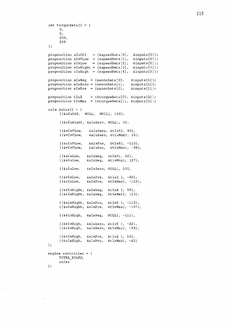
set torqueSets[] 0, 0, 255, 255
I ;
proposition sIsOii proposition sIsVLow
{&speedSets [0],
{&speedSet s (1] , {&speedSets (2], {&speedSets (3], { & speedSet s ( 4] ,
&inputs[O] ); &inputs [0]);
&inputs [0]);
&inputs(O]}; &inputs[O]};
proposition sIsLow proposition sIsRight proposition sIsHigh
proposition aIsNeg proposition aIsZero
{&accnSets (0], {&accnSets(1] , {&accnSet s [2],
&inputs[1] }; &input s [1] ); &inputs[1] ); proposition aIsPos
proposition tIsZ proposition tIsMax
rule rules[] = {
(&torqueSets[O] , &inputs(2]); {&torqueSets[1], &inputs(2]}i
{{&sIsOif, NULL, NULL}, 128},
{{&sIsRight, &aIsZero, NULL} , 0),
{ (&sIsVLow, &aIsZero, &tIsZL 99), { {&sIsVLow, &aIsZero, &tIsMax} , HI,
{ {&sIsVLow, &aIsPos, &tIsZ}, -115} , { {&sIsVLow, &aIsPos, &tIsMax} , -38) ,
{{&sIsLow, &aIsNeg, &tIsZ} , 62} , {{&sIsLow, &aIsNeg, &tIsMax} , 127},
{{&sIsLow, &aIsZero, NULL} , 10L
{ (&sIsLow, &aIsPos, &tIsZ ), -50) , { (&sIsLow, &aIsPos, &tIsMax) , -123),
{{&sIsRight, &aIsNeg, &tIsZ } , 58}, {{&sIsRight, &aIsNeg, &tIsMax} , 123) ,
{(&sIsRight, &aIsPos, &tIsZ ), -115} , {{&sIsRight, &aIsPos, &tIsMax} , -107L
{{&sIsHigh, &aIsNeg, NULL}, -111} ,
{{&sIsHigh, &aIsZero, &tIsZ }, -22}, { {& sI sHigh, &aIsZero, &tIsMax} , -99} ,
{ {& &aIsPos, &tIsZ }, 10 }, {{&sIsHigh, &aIsPos, &tIsMax} , -22)
} ;
engine controller TOTAL_RULES, rules
} i
115