Accepted Manuscript

Fuzzy differential equation with completely correlated parameters

V.M. Cabral, L.C. Barros

PII: S0165-0114(14)00374-1DOI: 10.1016/j.fss.2014.08.007Reference: FSS 6615

To appear in: Fuzzy Sets and Systems

Received date: 2 October 2012Revised date: 15 August 2014Accepted date: 18 August 2014

Please cite this article in press as: V.M. Cabral, L.C. Barros, Fuzzy differential equation withcompletely correlated parameters, Fuzzy Sets and Systems (2014),http://dx.doi.org/10.1016/j.fss.2014.08.007

This is a PDF file of an unedited manuscript that has been accepted for publication. As a service toour customers we are providing this early version of the manuscript. The manuscript will undergocopyediting, typesetting, and review of the resulting proof before it is published in its final form.Please note that during the production process errors may be discovered which could affect thecontent, and all legal disclaimers that apply to the journal pertain.

Fuzzy Differential Equation with Completely Correlated Parameters

V. M. Cabrala, L. C. Barrosb,∗

aDepartment of Mathematics, Federal University of Amazonas, Manaus, AM, BrazilbDepartment of Applied Mathematics, IMECC, University of Campinas, Campinas, SP, Brazil

Abstract

In this paper we study fuzzy differential equations with parameters and initial conditions interactive.The interactivity is given by means of the concept of completely correlated fuzzy numbers. We considerthe problem in two different ways: the first by using a family of differential inclusions; in the second theextension principle for completely correlated fuzzy numbers is employed to obtain the solution of the model.We conclude that the solutions of the fuzzy differential equations obtained by these two approaches are thesame. The solutions are illustrated with the radioactive decay model where the initial condition and thedecay rate are completely correlated fuzzy numbers. We also present an extension principle for completelycorrelated fuzzy numbers and we show that Nguyen’s theorem remains valid in this environment. In addition,we compare the solution via extension principle of the fuzzy differential equation when the parameters arenon-interactive fuzzy numbers and when the parameters are completely correlated fuzzy numbers. Finally,we study the SI-epidemiological model in two forms: first considering that the susceptible and infectedindividuals are completely correlated and then assuming that the transfer rate and the initial conditions arecompletely correlated.

Keywords: Completely Correlated Fuzzy Numbers; Extension Principle; Fuzzy Differential Inclusion;Fuzzy Differential Equation; SI-model.

1. Introduction

We begin by considering the initial value problem{x′(t) = f(x(t), w)x(t0) = x0,

(1)

where x0, w ∈ R and f is a continuous function.By making the change of variables y = (x,w), the initial value problem (1) may be rewritten as{

y′(t) = F (y(t))y(t0) = y0,

(2)

where F (y(t)) = (f(x(t), w), 0) and y0 = (x0, w).Supposing that x0 and w are uncertain and given by completely correlated fuzzy numbers X0 and W ,

y0 can be modeled by the joint possibility distribution C of X0 and W (see Section 2). So, it is possible torelate the deterministic problem (2) with the fuzzy initial value problem{

y′(t) = F (y(t))y(t0) ∈ C.

(3)

∗Corresponding authorEmail addresses: valtemircabral@yahoo.com.br (V. M. Cabral), laeciocb@ime.unicamp.br (L. C. Barros)

Preprint submitted to Elsevier August 20, 2014

The problem (3) is merely a notation, which can be approached in two different ways. The first approachis suggested by Hullermeier [1], in which the solution is given by the following family of differential inclusions:{

y′(t) = F (y(t))y(t0) ∈ [C]α.

(4)

where [C]α are the α-levels of the fuzzy subset C.The second approach is obtained by means of the application of the extension principle for completely

correlated fuzzy numbers to the deterministic solution of the problem (2) as made in [2, 3]. In Mizukoshiet al. [2] the study was made for the case that the joint possibility distribution C is given by the minimumt-norm of two fuzzy numbers, that is, the fuzzy numbers are non-interactive.

Oberguggenberger and Pittschmann in [3] studied the equation (1) for the case in which the coefficientsand initial conditions are fuzzy. They defined the operators fuzzy equation, fuzzy restriction and fuzzysolution of the equation (1) and apply the Zadeh’s extension principle in these operators as model forobtaining the solution of the fuzzy equation associated to the equation (1). Besides, they established theconcepts of fuzzy solution and for parts component fuzzy solution for the fuzzy differential equation insubject.

Bede and Gal in [4] presented a new approach to solve fuzzy differential equations. They introduced andstudied a new generalized concept of differentiability which extends usual known concept of differentiabilityof fuzzy-number-valued functions [5, 6, 7]. Following this idea, Chalco-Cano and Roman-Flores [8] introducedthe concept of fuzzy lateral H-derivative for fuzzy mapping and also demonstrated that the fuzzy solutionis equivalent to the solution via differential inclusion [9, 1].

J. Baetens and B. Baets [10] applied the concept of completely correlated fuzzy number for a discretemodel to study the evolution of a disease in space and time. Those approaches have been recently extendedto the case where two kinds of uncertainties, fuzziness and randomness, are present on the phenomenon.However, we do not threat this case here. This theory is called fuzzy stochastic differential equations, whichis based on stochastic differential equations. The reader can refer to [11, 12, 13, 14].

In section 2, we define the extension principle for completely correlated fuzzy numbers and show thatNguyen’s theorem [15] remains valid. In section 3, we show that a solution of (3) can be obtained throughextension principle, similarly to [2, 3]. We conclude that this fuzzy solution coincides with the solutionobtained by using Hullermeier’s approach, via differential inclusions. In order to exemplify we study theradioactive decay model with fuzzy intrinsic rate of decay and fuzzy initial conditions. In section 4, weapply the studied methods to the SI-model with susceptible individuals completely correlated with infectedindividuals and also considering the transfer rate completely correlated with the initial conditions.

2. Basic concepts

We denote by Kn the family of all the non-empty compact subsets of Rn. For A,B ∈ Kn and λ ∈ R theoperations of addition and scalar multiplication are defined by

A+B = {a+ b : a ∈ A, b ∈ B} and λA = {λa : a ∈ A}.A fuzzy subset A of Rn is given by a function

μA : Rn −→ [0, 1].

The α-levels or α-cuts of the fuzzy subset A are defined by

[A]α = {x ∈ Rn : μ

A(x) ≥ α} for 0 < α ≤ 1.

If α = 0, we define [A]0 = cl({x ∈ Rn : μA(x) > 0}), which is the closure of the support of A.

The family of the fuzzy subsets A, with [A]α ∈ Kn of Rn, will be denoted by F(Rn).The fuzzy subset A of the real line is a fuzzy number if all the α-levels of A are non-empty closed intervals

of R and the support of Asupp(A) = {x ∈ R : μ

A(x) > 0}

2

is bounded.We denote by E(R) the family of the fuzzy numbers.The following definition can be found in [16].

Definition 2.1. An n-dimensional possibility distribution on Rn is a fuzzy subset C with membership func-

tion μC: Rn −→ [0, 1] satisfying μ

C(x0) = 1 for some x0 ∈ R

n.

The family of the n-dimensional possibility distribution will be denoted Fc(Rn).

Definition 2.2. Let A1, A2, ..., An ∈ E(R) be fuzzy numbers, then C ∈ Fc(Rn) is called a joint possibility

distribution if

μAi(xi) = max

xj∈R, j �=iμC(x1, x2, ..., xn), ∀xi ∈ R, i = 1, 2, ..., n.

Furthermore, μAi is called the i-th marginal possibility distribution of C.

Definition 2.3. The fuzzy numbers A1, A2, ..., An ∈ E(R) are said to be non-interactive if and only if theirjoint possibility distribution C is given by

μC (x1, x2, ..., xn) = min{μA1(x1), μA2

(x2), ..., μAn(xn)}

for all x = (x1, x2, ..., xn) ∈ Rn, or equivalently,

[C]α = [A1]α × [A2]

α × ...× [An]α,

for all α ∈ [0, 1].

On the other hand, A1, A2, ..., An ∈ E(R) are said to be interactive if they cannot take their valuesindependently of each other [17, 18].

Definition 2.4. The fuzzy numbers A1, A2, ..., An ∈ E(R) are said to be weakly non-interactive accordingto the t-norm T if and only if their joint possibility distribution C is given by

μC (x1, x2, ..., xn) = T (μA1(x1), μA2

(x2), ..., μAn(xn))

for all x = (x1, x2, ..., xn) ∈ Rn.

In Definition 2.5 we present an important class of interactive fuzzy numbers called completely correlated[19, 17]. Applications of this concept appear in [20, 10].

Definition 2.5. Two fuzzy numbers A and B are said to be completely correlated if there exist q, r ∈ R,with q �= 0, such that their joint possibility distribution is given by

μC (x, y) = μA(x)X{qx+r=y}(x, y) (5)

= μB(y)X{qx+r=y}(x, y)

where

X{qx+r=y}(x, y) ={

1 if qx+ r = y0 if qx+ r �= y

is the characteristic function of the line {(x, y) ∈ R2 : qx+ r = y}.

In this case we have:

[C]α = {(x, qx+ r) ∈ R2 : x = (1− s)aα1 + saα2 , s ∈ [0, 1]}

where [A]α = [aα1 , aα2 ]; [B]α = q[A]α + r, for any α ∈ [0, 1] Moreover, if q �= 0,

μB(x) = μA(x− r

q), ∀x ∈ R.

3

In Definition 2.5 if q is positive (negative), the fuzzy numbers A and B are said to be completely positively(negatively) correlated. In this case, if [B]α = q[A]α + r, then the correlated addition of A and B is thefuzzy number A+B with α-cuts

[A+B]α = (q + 1)[A]α + r. (6)

In what follows, we will formulate the extension principle for completely correlated fuzzy numbers [19] .

Definition 2.6. Let C be a joint possibility distribution with marginal possibility distributions A and B,and let f : R2 −→ R

2 be a continuous function. If A and B are completely correlated fuzzy numbers, thenthe extension of f applied in (A,B) is the fuzzy set f

C(A,B) whose membership function is defined by

μfC

(A,B)(u, v) =

⎧⎪⎨⎪⎩sup

(x,y)∈f−1(u,v)

μC(x, y), if f−1(u, v) �= ∅

0 , if f−1(u, v) = ∅,

where f−1(u, v) = {(x, y) : f(x, y) = (u, v)}.

The next theorem can be interpreted as a generalization of Nguyen’s theorem [15].

Theorem 2.7. Let A,B ∈ E(R) be completely correlated fuzzy numbers, let C be their joint possibilitydistribution, and let f : R2 −→ R

2 be a continuous function. Then,

[fC(A,B)]α = f([C]α).

Proof: Let g : R −→ R2 be the continuous function g(x) = f(x, qx+ r).

We will divide the proof in two cases: α > 0 and α = 0.1) For α > 0.

Let (u, v) ∈ f([C]α), then there exist (x0, y0) ∈ [C]α, with μC(x0, y0) ≥ α and (u, v) = f(x0, y0). Then

μfC

(A,B)(u, v) = sup

(x,y)∈f−1(u,v)

μC (x, y) ≥ μC (x0, y0) ≥ α,

that is,(u, v) ∈ [fC (A,B)]α.

Reciprocally, let (u, v) ∈ [fC (A,B)]α, then

μfC

(A,B)(u, v) = sup

(x,y)∈f−1(u,v)

μC(x, y) ≥ α,

so that f−1(u, v) �= ∅.Now,

μfC

(A,B)(u, v) = sup

(x,y)∈f−1(u,v)

μC(x, y)

= sup(x,y)∈f−1(u,v)

μA(x)X{qx+r=y}(x, y)

= sup(x,xq+r)∈f−1(u,v)

μA(x)X{qx+r=y}(x, xq + r)

= supx∈g−1(u,v)

μA(x)

= supx∈[A]0∩g−1(u,v)

μA(x)

= μA(x1) ≥ α,

4

for some x1 ∈ [A]0 ∩ g−1(u, v) since μA is upper semicontinuous and [A]0 ∩ g−1(u, v) is a compact set of R.Thus, (u, v) ∈ f([C]α).

2) For α = 0.Consider U = {(u, v) : μ

fC

(A,B)(u, v) > 0} and V = {(u, v) : μ

C(u, v) > 0}.

We will show that U = f(V ), where U = cl(U).Let (u, v) ∈ U , then μ

fC

(A,B)(u, v) = sup

(x,y)∈f−1(u,v)

μC(x, y) > 0. Hence there exists (a, b) ∈ R

2 with

f(a, b) = (u, v) and μC(a, b) > 0. Therefore

(u, v) ∈ f(V ) and U = f(V ).

Thus,

U ⊂ f(V ) ⊂ f(V ) = f(V ),

because V is compact and f is continuous.On the other hand, let (u, v) ∈ f(V ). Then there exists (a, b) ∈ V such that f(a, b) = (u, v) and

μC (a, b) > 0.And since sup

(x,y)∈f−1(u,v)

μC (x, y) ≥ μC (a, b) > 0, we have (u, v) ∈ U .

Thus,f(V ) ⊂ f(V ) ⊂ U,

because f is continuous. �

2.1. Differential Inclusion

Consider the following differential inclusion,{x′(t) ∈ F (t, x(t))

x(t0) = x0 ∈ X0,(7)

where F : [t0, T ]× Rn −→ Kn is a set-valued function and X0 ∈ Kn.

A function x(., x0), with x0 ∈ X0, is a solution of (7) in interval [t0, T ] if it is absolutely continuous andsatisfies (7) for almost all t ∈ [t0, T ]. The attainable set at time t ∈ [t0, T ], associated to problem (7), is thesubset of Rn given by

At(X0) = {x(t, x0) : x(., x0) is solution of (7) }.The set-valued function F allows the modeling of some types of uncertainty, because for each pair

(t, x) ∈ [t0, T ] × Rn, the derivative cannot be precisely known, but the derivative is an element of the set

F (t, x).A generalization of problem (7), to model fuzzy dynamical systems, is obtained by replacing the set

F (t, x) in (7) by a fuzzy set, that is, we consider the fuzzy initial value problem{x′(t) ∈ F (t, x(t))

x(t0) = x0 ∈ X0,(8)

where F : [t0, T ]× Rn −→ F(Rn) is a fuzzy set-valued function and X0 ∈ F(Rn).

In agreement with Hullermeier [1], the problem (8) is interpreted as the family of differential inclusions{x′(t) ∈ [F (t, x(t))]α

x(t0) = x0 ∈ [X0]α,

(9)

where [F (t, x(t))]α are the α-levels of fuzzy set F (t, x(t)).In order to simplify the notation, we will denote by X0 the fuzzy set of the initial condition.For each α ∈ [0, 1], we say that xα : [t0, T ] −→ R

n, is an α-solution of (8) if it is a solution of (9).The attainable set of the α-solutions will be denoted by At([X0]

α) := Aαt , t0 ≤ t ≤ T , that is,

5

Aαt = At([X0]

α) = {xα(t, x0) : xα(., x0) is a solution of (9)}.Aα

t are the α-levels of a fuzzy set At(X0) ∈ F(Rn) for all t0 ≤ t ≤ T (for more details, see [9]). The fuzzyset At(X0) is named the attainable set of problem (7).

3. Differential equations with fuzzy coefficient and fuzzy initial condition

In this section we will study the fuzzy differential equations with both coefficient and initial conditionuncertain and modeled by completely correlated fuzzy numbers. The fuzzy differential equations are obtainedfrom deterministic differential equations by introducing the uncertain elements mentioned. Mizukoshi et al.[2] studied this problem supposing that the coefficient and the initial condition were non-interactive.

We begin with the initial value problem{x′(t) = f(x(t), w)x(t0) = x0,

(10)

where f is a continuous function and x0, w ∈ R.By making the change of variables y = (x,w), the initial value problem (10) may be rewritten as{

y′(t) = F (y(t))y(t0) = y0,

(11)

where y′(t) = (x′(t), 0), F (y(t)) = (f(x(t), w), 0), and y0 = (x0, w).Supposing that x0 and w are uncertain and modeled by completely correlated fuzzy numbers X0 and

W , the problem (11) is replaced by {y′(t) = F (y(t))y(t0) = (x0, w) ∈ C,

(12)

where C is the joint possibility distribution of the completely correlated fuzzy numbers X0 and W .

3.1. Solution via extension principle

Let U be an open subset of R2 such that there exists a unique solution y(., y0) of (11) with y0 ∈ U andfor all t ∈ [t0, T ], y(t, .) is continuous in U . Consider the operator

Lt : U −→ R2,

with Lt(y0) = y(t, y0), which is the unique solution of (11) and is continuous with respect to y0.The solution of problem (12), via extension principle, is given by the operator (Lt)C which is obtained

applying the extension principle in the operator Lt.The following theorem presents a relation between the solutions of the problem (12) when X0 and W

are non-interactive fuzzy numbers and when X0 and W are completely correlated fuzzy numbers.

Theorem 3.1. Suppose that for every (x0, w) ∈ R2 there is a unique solution to the problem (11) in the

interval [t0, T0]. Then, the solution of the problem (12) via extension principle when X0 and W are non-interactive, and when X0 and W are completely correlated satisfies the following relation

[(Lt)C(X0,W )]α ⊆ [(Lt)TM(X0,W )]α, ∀α ∈ [0, 1],

where TM (x0, w) = min(μX0(x0), μW (w)), that is, TM is the joint possibility distribution of the non-interactive fuzzy numbers X0 and W .

Proof: From Theorem 2.7,

[(Lt)C(X0,W )]α = Lt([C]α) = {Lt(x0, w) : (x0, w) ∈ [C]α}= {Lt(x0, qx0 + r) : x0 ∈ [X0]

α, for some r and q �= 0}⊂ {Lt(x0, w) : (x0, w) ∈ [X0]

α × [W ]α}= [(Lt)TM

(X0,W )]α.

(13)

It is clear that if (11) is deterministic, that is, X0 and W are real numbers, the (Lt)C = (Lt)TM.

6

3.2. Solution via differential inclusions

The problem (12), according to Hullermeier’s interpretation, can be written as a family of differentialinclusions {

y′(t) = F (y(t))y(t0) ∈ [C]α.

(14)

Following Diamond [9], the attainable sets Aαt = At([C]α) are the α-levels of a fuzzy set At(C), where

At(C) ⊂ R2, for each α ∈ [0, 1] and each t ∈ [t0, T ].

At this point we are able to state the following theorem.

Theorem 3.2. Let U be an open subset in R2 and C the joint possibility distribution of X0,W ∈ F(R).

Suppose that F , in (12), is a continuous function, that for each y0 = (x0, w) ∈ U there exists an uniquesolution y(., y0) of the problem (11) and that y(t, .) is continuous in U . Then, for all t ∈ [t0, T ] we have

(Lt)C (X0,W ) = At(C).

In words, the solution via differential inclusions of (11) and the solution via extension principle coincide.

Proof: In order to prove this result we must show that

[(Lt)C (X0,W )]α = At([C]α), ∀α ∈ [0, 1].

We have that F is a continuous function and for each y0 = (x0, w) ∈ U there exists a unique solutionfor the problem (11) in the interval [t0, T ]. Consequently, for each t ∈ [t0, T ], the operator Lt : U −→ R

2

defined by Lt(y0) = y(t, y0) is the unique solution of the problem (11) and it is continuous relative toy0 = (x0, w). Then, the operator (Lt)C is the solution of the problem (12), via extension principle andaccording to Theorem 2.7, we have

[(Lt)C (X0,W )]α = Lt([C]α), ∀α ∈ [0, 1].

Given α ∈ [0, 1], we can write

At([C]α) = {(y(t, y0) : y(., y0) is solution of (11) }= {(y(t, y0) : y′(t) = F (y(t)), y0 = (x0, w) ∈ [C]α}= {Lt(y0) : y0 = (x0, w) ∈ [C]α}= Lt([C]α).

(15)

Hence [(Lt)C(X0,W )]α = Lt([C]α) = At([C]α).

Example 3.3. (Radioactive decay model with uncertain decay rate and initial condition)

Here we consider a radioactive decay model where the decay rate and the initial conditions are interactivefuzzy numbers. This interaction is due to the fact that (intuitively) an amount of radioactive substancewith big initial condition presents big rate of decay. In this example the interactivity is given by means ofcompletely correlated fuzzy numbers, according to definition 2.5.

Let us consider the problem {x′(t) = wx(t)x(0) = x0,

(16)

where w is the decay rate and x0 is the initial condition. The problem (16) may be rewritten as{(x′(t), w′(t)) = (wx(t), 0)(x(0), w(0)) = (x0, w).

(17)

Suppose that x0 and w are uncertain and modeled by completely correlated triangular fuzzy numbersX0 = (2; 3; 4) and W = (−2;−1; 0). Then, the joint possibility distribution C is given by

μC(x0, w) = μX0(x0)X{x0+w=2}(x0, w) (18)

7

= μW (w)X{x0+w=2}(x0, w).

Problem (17) is replaced by {(x′(t), 0) = (wx(t), 0)(x0, w) ∈ C

(19)

and problem (19) is interpreted as {(x′(t), 0) = (wx(t), 0)(x0, w) ∈ [C]α

(20)

with [X0]α = [α+2, 4−α], [W ]α = [α−2,−α] and [C]α = {(x0, 2−x0) ∈ R

2 : x0 = (1−s)(α+2)+s(4−α),s ∈ [0, 1]}.

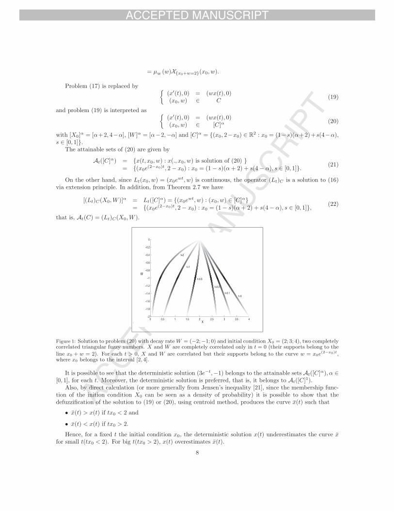
The attainable sets of (20) are given by

At([C]α) = {x(t, x0, w) : x(., x0, w) is solution of (20) }= {(x0e

(2−x0)t, 2− x0) : x0 = (1− s)(α+ 2) + s(4− α), s ∈ [0, 1]}. (21)

On the other hand, since Lt(x0, w) = (x0ewt, w) is continuous, the operator (Lt)C is a solution to (16)

via extension principle. In addition, from Theorem 2.7 we have

[(Lt)C(X0,W )]α = Lt([C]α) = {(x0ewt, w) : (x0, w) ∈ [C]α}

= {(x0e(2−x0)t, 2− x0) : x0 = (1− s)(α+ 2) + s(4− α), s ∈ [0, 1]}, (22)

that is, At(C) = (Lt)C(X0,W ).

0 0.5 1 1.5 2 2.5 3 3.5 4−2

−1.8

−1.6

−1.4

−1.2

−1

−0.8

−0.6

−0.4

−0.2

0

W

X

t=0

t=0.2

t=0.1

t=0.5

t=1

t=2

Figure 1: Solution to problem (20) with decay rateW = (−2;−1; 0) and initial conditionX0 = (2; 3; 4), two completelycorrelated triangular fuzzy numbers. X and W are completely correlated only in t = 0 (their supports belong to the

line x0 + w = 2). For each t > 0, X and W are correlated but their supports belong to the curve w = x0e(2−x0)t,

where x0 belongs to the interval [2, 4].

It is possible to see that the deterministic solution (3e−t,−1) belongs to the attainable sets At([C]α), α ∈[0, 1], for each t. Moreover, the deterministic solution is preferred, that is, it belongs to At([C]1).

Also, by direct calculation (or more generally from Jensen’s inequality [21], since the membership func-tion of the inition condition X0 can be seen as a density of probability) it is possible to show that thedefuzzification of the solution to (19) or (20), using centroid method, produces the curve x(t) such that

• x(t) > x(t) if tx0 < 2 and

• x(t) < x(t) if tx0 > 2.

Hence, for a fixed t the initial condition x0, the deterministic solution x(t) underestimates the curve xfor small t(tx0 < 2). For big t(tx0 > 2), x(t) overestimates x(t).

8

4. The fuzzy SI-model

The simplest mathematical model that describes the dynamics of diseases transmitted by direct contactbetween susceptible and infected individuals is called SI [22, 23, 24]. In this model the individual does notrecover from the disease. A typical example is AIDS, wherein once infected by the virus, the individual willremain with it for the rest of his life.

In the study we will consider uncertain parameters modeled by completely correlated fuzzy numbers.We will analyse the model using the two techniques already presented this article: via differential inclusionand via principle of extension.

Usually, the SI-model is described by the system of differential equations⎧⎪⎪⎪⎨⎪⎪⎪⎩dS

dt= −mSI, S(0) = S0

dI

dt= mSI, I(0) = I0 > 0,

(23)

where S(t) and I(t) are, respectively, the fractions of susceptible and infected individuals at the time t. Theparameter m is a positive constant representing the rate of contact of the disease.

Suppose that there is no variation in the total number of the population, i.e., consider the model withoutvital dynamics:

S(t) + I(t) = 1, ∀t ≥ 0. (24)

Thus, S(t) = 1− I(t) and replacing in the system (23), we get⎧⎪⎨⎪⎩dI

dt= m(1− I)I

I(0) = I0 > 0

, (25)

whose solution is given by

I(t) =I0e

mt

S0 + I0emtand S(t) = 1− I(t) =

S0

S0 + I0emt. (26)

Therefore, for each t ≥ 0, the deterministic solution of the problem (23) is given by

Lt(S0, I0) =

(S0

S0 + I0emt,

I0emt

S0 + I0emt

). (27)

4.1. The SI-model with completely correlated initial conditions

We will consider in the system (23) that the initial conditions are uncertain and modeled by fuzzynumbers. Since S0 + I0 = 1, we are dealing with completely correlated fuzzy numbers with r = 1 andq = −1. This means that the joint possibility distribution C of S0 and I0 is such that

μC(s0, i0) = μS0(s0)X{s0+i0=1}(s0, i0) = μI0(i0)X{s0+i0=1}(s0, i0). (28)

In the case, for each α ∈ [0, 1], we have

μI0(i0) = μS0

(1− i0), [I0]α = [aα1 , a

α2 ], [S0]

α = (−1)[I0]α + 1

and[C]α = {(1− i0, i0) ∈ R

2 : i0 = (1− γ)aα1 + γaα2 , γ ∈ [0, 1]}. (29)

Thus, according to Formula (6), S0 + I0 = 1, since q = −1 and r = 1.

9

Taking into consideration (28), the equation (23) becomes⎧⎪⎪⎨⎪⎪⎩(dS

dt,dI

dt

)=

(−mSI,mSI

)(I0, S0) ∈ C

. (30)

Solution of the fuzzy SI-model via differential inclusion

In order to obtain the solution to the equation (30) via fuzzy differential inclusion, we will apply themethod described in subsection 3.2.

The solution of the problem (30), using differential inclusion, is obtained from the solution of the auxiliaryproblem ⎧⎨⎩ (dSdt ,

dIdt ) = (−mSI,mSI)

(S0, I0) ∈ [C]α,(31)

where [C]α is given by equation (29).The attainable sets of the problem (31) are given by

At([C]α) =

{x(t, S0, I0) : x(., S0, I0) is solution of (31)

}=

{x(t, S0, I0) : x

′(t, S0, I0) = (−mSI,mSI), (S0, I0) ∈ [C]α}

=

{(s0

s0+i0emt ,i0e

mt

s0+i0emt

): (s0, i0) ∈ [C]α

}=

{(1−i0

(1−i0)+i0emt ,i0e

mt

(1−i0)+i0emt

): i0 = (1− γ)aα1 + γaα2 , γ ∈ [0, 1]

}.

(32)

Solution of the fuzzy SI-model via extension principle

We will study the fuzzy SI-model given by equation (30) using as tool the extension principle via Defi-nition 2.6. In this case, the solution is obtained by applying the extension principle using Definition 2.6 inEquation (27).

According to Theorem 2.7 the α-levels of the solution obtained by the extension principle of the problem(30) are given by the expression

[(Lt)C(S0, I0)]α = Lt([C]α).

Therefore, the α-levels of the solution of the problem (30) are

[(Lt)C(S0, I0)]α = Lt([C]α)

=

{Lt(s0, i0) : (s0, i0) ∈ [C]α

}=

{Lt(1− i0, i0) : i0 = (1− γ)aα1 + γaα2 , γ ∈ [0, 1]

}=

{(1−i0

(1−i0)+i0emt ,i0e

mt

(1−i0)+i0emt

): i0 = (1− γ)aα1 + γaα2 , γ ∈ [0, 1]

}.

(33)

That is, as predicted by Theorem 3.2, for every t ≥ 0, the sets (Lt)C(S0, I0) and At(C) are identical.Figure 2 represents the solution to the problem (30) employing the completely correlated triangular fuzzy

numbers I0 = (0.05; 0.08; 0.11) and S0 = (0.89; 0.92; 0.95) as initial conditions, with S0 + I0 = 1 (accordingto Formula (6)), and contact rate m = 0.3.

10

Figure 2: Fuzzy solution to the problem (30) in the phase-portrait. The dots correspond to the deterministic solutionfor different values of time t. The initial conditions are the completely correlated triangular fuzzy numbers I0 =(0.05; 0.08; 0.11) and S0 = (0.89; 0.92; 0.95), with S0 + I0 = 1, and the contact rate is m = 0.3. Darker regions (foreach t ≥ 0) mean greater possibility (membership) of the number of susceptible and infected to the solution of theproblem. The deterministic solution has membership degree equal to 1 in the fuzzy solution.

The fact that the fuzzy numbers are completely correlated makes the solution to the problem (30) be acurve contained in the line S + I = 1, for each t ≥ 0.

A study about interactivity between the contact rate (m) and the initial condition (I0) can be made.The justification for this consideration is similar to the one argumented in Example 3.3, that is, the biggerthe initial condition, the smaller the contact rate. The analysis of the solution is made in a similar form towhat has been done to the solution of the SI model above. For this specific case, the force of infection f(the probability of a susceptible individual being infected per unit of time) is given by f = m · I. For t = 0,we have f = m · I0.

Barros et al. [22] also studied the SI model with contact rate given by fuzzy number, but not consideringI0 fuzzy. So, there was no interactivity between the initial condition I0 and m. They have concluded that,with this hypothesis, it is possible to show that the number of infected individuals given by the deterministicmodel and that one from the fuzzy model become very different.

4.2. Number of Infected Individuals via classical and fuzzy models

First, notice that both the deterministic and the fuzzy solutions to (23) belong to the line S + I = 1.While the deterministic solution has precise values for each t, the fuzzy solution is given by possibilitydistributions on the line S+ I = 1. However, it is possible to show that the former is preferred to the latter,i. e., for each t > 0, the former belongs to the later with membership equal to 1 (see Figure 2).

Our main goal in this subsection is to compare the number of individuals predicted by both models:deterministic and fuzzy. For this we need to have a deterministic curve obtained from the fuzzy solution.

Since the initial conditions are uncertain and modeled by completely correlated fuzzy numbers, a com-parison between infected individuals number, given by both the classical model and the fuzzy model, is onlypossible if the fuzzy solution is “defuzzified”. We will do it just to case where the intial conditions are fuzzy,that is, we will not study the case where the contact rate is fuzzy.

Thus, according to Formula (26), for each t > 0 consider the number of infected individuals

It(I0) =I0e

mt

(1− I0) + I0emt,

where m is the contact rate.

11

The defuzzification for It(I0), given by the centroid method is

E[It(I0)] =

∫RIt(i0)μI0(i0)di0∫RμI0(i0)di0

(34)

whose value depends of membership function μI0 adopted for fuzzy set I0.Formula (34) can be seen as the Classical Expectancy of Infected Individuals whose probability density

function isμI0(i0)∫

RμI0(i0)di0

.

Since the function

gt(x) =xemt

(1− x) + xemt,

for each t > 0 and m > 0, is a strictly concave function, according to Jensen’s inequality [21], we have

E[It(I0)] < It[E(I0)]. (35)

Note that It[E(I0)] represents the number of infected individuals of the deterministic model, where theaverage of I0 (E(I0)), is the initial condition. So, if we adopt the deterministic curve x(t) = E[It(I0)] topredict the number of infected, it is possible to conclude that the curve given by expectancy of fuzzy solutionis smaller than the one given by the deterministic model.

A defuzzification procedure, at appropriate moment t, makes the fuzzy model more general than thedeterministic one. The deterministic case does not admit any kind of uncertainty and, consequently, thedefuzzification is necessary at t = 0. So, the defuzzification of initial condition at t = 0 yields the determin-istic solution It[E(I0)] to represent the evolution of the disease. However, as we have seen in the previoussection, It[E(I0)] is very different from the expectancy (E[It(I0)]) of the fuzzy solution.

5. Final considerations

The SI-epidemiologial model is traditionally studied assuming that the transfer rate and the initialconditions are real numbers. Moreover, there are no hypothesis about the interaction between these pa-rameters. In this paper, we have explored the SI-model with the hypothesis that the parameters are givenby interactive fuzzy numbers. In this case, the solution obtained via the extension principle is contained inthe solution that has non-interactive fuzzy parameters. In other words, the solution with interactive fuzzyparameters is less fuzzy than the solution with non-interactive parameters.

We have also studied the radioative decay model (Example 3.3) with interactive rate and initial condition.Mizukoshi et al. in [2] studied the same model assuming that these parameters are non-interactive. Thesolution with non-interactive parameters is more fuzzy than the solution with interactive parameters. Fur-thermore, the solution obtained via the differential inclusion of the decay model coincides with the solutionobtained via the extension principle.

Finally, we compared the quantities predicted from both methods, deterministic and fuzzy. For theExample 3.3 of radioactive decay, in the beginning of the process the fuzzy model predicts bigger value thanthe deterministic one. At the end of the process, the opposite has happened. On the other hand, for the SImodel, according to (35) the deterministic case predicts bigger values than the fuzzy case, for all t > 0.

Acknowledgements

The authors would like to thank CNPq (Brazil) for providing the financial support needed in this research(grant No. 305862/2013-8).

12

References

[1] E. Hullermeier, An approach to modelling and simulation of uncertain dynamical systems, Int. J. Uncertainty, FuzzinessKnowledge-Bases Syst. 5 (2) (1997) 117–137.

[2] M. T. Mizukoshi, L. C. Barros, Y. Chalco-Cano, H. Roman-Flores, R. C. Bassanezi, Fuzzy differential equations and theextension principle, Information Sciences 177 (2007) 3627–3635.

[3] M. Oberguggenberger, S. Pittschmann, Differential equations with fuzzy parameters, Math. Mod. Systems 5 (1999) 181–202.

[4] B. Bede, S. Gal, Generalizations of the differentiability of fuzzy-number-valued functions with applications to fuzzydifferential equations, Fuzzy set and systems 151 (2005) 581–599.

[5] B. Bede, S. Gal, Almost periodic fuzzy-number-valued functions, Fuzzy Sets and Systems 147 (2004) 385–403.[6] G. A. Anastassiou, On H-fuzzy differentiation, Math. Balkanica 16 (2002) 155–193.[7] C. Wu, Z. Gong, On Henstock integral of fuzzy-number-valued functions, Fuzzy Sets and Systems 120 (2001) 523–532.[8] Y. Chalco-Cano, H. Roman-Flores, On new solutions of fuzzy differential equations, Chaos, solitons and fractals 38 (2008)

112–119.[9] P. Diamond, Time-dependent differential inclusions, cocycle attractors an fuzzy differential equations, IEEE Trans. Fuzzy

Systems 7 (1999) 734–740.[10] J. M. Baetens, B. D. Baets, Incorporating fuzziness in spatial susceptible-infected epidemic models, in: Proceeding of

IFSA-EUSFLAT Conference, Lisbon, Portugal, CD-ROM, 2009.[11] S. Busenberg, P. van Driessche, Analysis of a disease transmission model in a population with varying size, J. Math. Biol.

28 (1990) 257–270.[12] M. T. Malinowski, M. Michta, Fuzzy stochastic integral equations, Dynam. Systems Appl. 19 (2010) 473–494.[13] M. Michta, Set-valued stochastic integrals and fuzzy stochastic equations, Fuzzy Sets and Systems 177 (2011) 1–19.[14] M. T. Malinowski, M. Michta, Stochastic fuzzy differential equations with an application, Kybernetika 47 (2011) 123–143.[15] H. T. Nguyen, A note on the extension principle for fuzzy sets, J. Math. Analysis and Applications 64 (1978) 369–380.[16] C. Carlsson, R. Fuller, On possibilistic mean value and variance of fuzzy numbers, Fuzzy sets and systems 122 (2001)

315–326.[17] C. Carlsson, R. Fuller, T. Keresztfalvi, On Possibilistic correlation, Fuzzy Sets and Systems 155 (2005) 425–445.[18] D. Dubois, H. Prade, Additions of Interactive Fuzzy Numbers, IEEE Transaction on Automatic Control 26 (1981) 926–936.[19] C. Carlsson, R. Fuller, T. Keresztfalvi, Additions of completely correlated fuzzy numbers, in: Fuzzy IEEE 2004 CD-ROM

Conference Proceedings, Budapest, 26–29, 2004.[20] M. Z. Ahmad, B. D. Baets, A predator-prey model with fuzzy initial populations, in: Proceeding of IFSA-EUSFLAT

Conference, Lisbon, Portugal, CD-ROM, 2009.[21] S. M. Ross, A first course in probability, Prentice Hall, Upper Saddle River, N.J., 2010.[22] L. C. Barros, R. C. Bassanezi, M. B. F. Leite, The epidemiological model SI with a fuzzy transmission parameter, Computer

and Mathematics with Applications 45 (2003) 1619–1628.[23] L. Edelstein-Keshet, Mathematical models in biology, Classics in applied mathematics, SIAM, Philadelphia, 2005.[24] J. D. Murray, Mathematical Biology I. An Introduction, vol. 1, Springer, New York, 2002.

13