fuzzy: a program for performing qualitative comparative...

The Stata Journal (2008)8, Number 1, pp. 79–104

fuzzy: A program for performing qualitativecomparative analyses (QCA) in Stata

Kyle C. LongestDepartment of Sociology

University of North Carolina at Chapel HillChapel Hill, NC

[email protected]

Stephen VaiseyDepartment of Sociology

University of North Carolina at Chapel HillChapel Hill, NC

Abstract. Qualitative comparative analysis (QCA) is an increasingly popularanalytic strategy, with applications to numerous empirical fields. This articlebriefly discusses the substantive motivation and technical details of QCA, as wellas fuzzy-set QCA, followed by an in-depth discussion of how the new programfuzzy performs these techniques in Stata. An empirical example is presented thatdemonstrates the full suite of tools contained within fuzzy, including creatingconfigurations, performing a series of statistical tests of the configurations, andreducing the identified configurations.

Keywords: st0140, fuzzy, cmvom, cnfgen, coincid, coverage, fzplot, mavmb, re-duce, setgen, suffnec, truthtab, yavyb, yvn, yvo, yvv, yvy, qualitative comparativeanalysis, QCA, fuzzy sets, Boolean logic, Boolean data, postestimation command

1 Introduction

In recent years, researchers in a number of fields have begun using qualitative compar-ative analysis (QCA) or its fuzzy-set variant to analyze multivariate data (Ragin 1987,2000). For examples, see Kalleberg and Vaisey (2005), Mahoney (2003), Roscigno andHodson (2004), and Vaisey (2007). Rather than estimate the net effects of single vari-ables, QCA employs Boolean logic to examine the relationship between an outcome andall binary combinations of multiple predictors. The advantage of QCA is that it allowsthe researcher to find distinct combinations of causal variables that, in turn, suggest dif-ferent theoretical pathways to given outcomes. Although early versions of QCA (Ragin1987) were criticized on the grounds that they were deterministic and that they bore lit-tle relation to commonly used variants of the general linear model, recent developmentsare now integrating QCA-based strategies with more formal statistical distributions andprocedures (Ragin 2006; Smithson and Verkuilen 2006).

c© 2008 StataCorp LP st0140

80 fuzzy: A program for performing QCA in Stata

2 Why QCA?

Because QCA is still a relatively new strategy, we illustrate its utility by describing onesubstantive topic that might benefit from its application. The stress process model hasinspired a wealth of research in the mental health field that has shown the deleteriousconsequences of an accumulation of stressors on increased negative health outcomes. Yetpersonal resources, active coping strategies, and social support can buffer these stressors,thereby reducing their harmful impact (for reviews, see Lin and Ensel [1989] and Thoits[1995]). The strength of this research notwithstanding, Thoits (1995) argued that theremay be important pathways to negative health outcomes that have remained unseenbecause investigators typically apply linear estimation models to the stress process.

Just as there may be different combinations of conditions across countrieswhich lead to political revolution, there may be different configurations offactors across individuals which lead to heart attack or to the onset of majordepression. . . . The assumption of one process for becoming depressed or illand the concomitant use of the general linear model to test it requires us toreject or ignore other possible processes which are less frequently observedand do not manage to achieve statistical significance. (Thoits 1995, 68)

In this observation, Thoits was advocating the use of QCA in tests of the stressprocess model. That is, high levels of conjunction among stressors and buffering agentscould define multiple routes to the same level of distress.

In addition to finding multiple paths to an outcome, QCA is especially appropri-ate for testing models, like that underlying stress theory, that involve a multitude of“interacting” factors. More precisely, QCA effectively addresses theoretical hypothesesthat predict multiple variables will operate in tandem at specific levels (e.g., high stressevents, low coping resources, and low social support) to produce particular outcomes(e.g., high distress). For example, stress theory predicts that numerous negative eventsshould interact with chronic strain to produce high levels of distress, but the use of sev-eral active coping strategies should moderate this interaction, reducing the likelihood ofelevated distress. Furthermore, high levels of mastery may enhance the buffering influ-ence of active coping efforts, and high social support might further increase mastery’smoderating influence on the interaction of active coping with stressors. This hypothesismodeled in a regression framework would involve a five-way interaction term, whichwould have to be interpreted along with all of its component interactions, an obviouslydifficult and inefficient task. QCA, on the other hand, explicitly and straightforwardlytests each possible combination of factors at specific levels with a given outcome. Theresults then can be interpreted more clearly, making QCA a potentially more effectiveanalytic strategy for complex theoretical processes such as those posed by stress theory.

The stress process model is just one specific case that would benefit from the ap-plication of QCA.1 QCA’s utility as an analytic strategy stands to augment research innumerous fields. Greckhamer and his colleagues (2007) have recently argued for QCA’s

1. Longest and Thoits (2007) have tested this model with QCA and found several intriguing results.

K. C. Longest and S. Vaisey 81

application in strategic management research because of its ability to analyze complexrelationships between different industry- and corporate-level mechanisms in predictingbusiness success. Similarly, researchers in epidemiology would benefit from QCA’s capac-ity to capture holistically individuals’ experience of risk and protective characteristics(Schuit et al. 2002). Finally, Shanahan et al. (2007) have demonstrated how QCA canbe employed to examine the complex relationship between environmental and geneticfactors leading to adult success.

We believe that part of the reason QCA has not been utilized more widely in empiricalresearch across fields is because no software presently exists that easily combines QCA

with conventional data management and statistical tests. The primary stand-aloneprogram, fuzzy-set QCA, is able to compute logical truth tables for both fuzzy-set anddichotomous-set data, but it has no built-in capacity for probabilistically testing logicalnecessity and sufficiency, as advocated by Ragin (2006). There is also a program for theR statistics language that can perform logical reductions of Boolean data, but it lacksthe ability to perform useful statistical tests. Further, there is no program in Stata thatcan perform the necessary analyses or reductions in fuzzy-set analyses.

In this paper, we present and outline fuzzy, a new Stata command we have developedthat is capable of creating, testing, and performing logical reductions on both fuzzy anddichotomous (crisp) set-theoretic data. We will first outline some of the backgroundof the technique and then provide a detailed explanation of the functionality of thecommand.

3 Statistical background

QCA evaluates the relationship between an outcome and all possible Boolean combina-tions of predictors. For example, given an outcome set Y and predictor sets A and B,QCA examines which combinations of A and B (i.e, A · B, A · b, a · B, a · b) are most likelyto produce Y. In a QCA framework, the term “set” is used rather than “variable” to em-phasize the idea that each variable has been transformed to represent the individual’slevel of membership in a given condition, for example, his or her level of membershipin “heavy alcohol users”. The combination of individual “sets”—for example, high de-pression and low self esteem—is then referred to as a “configuration”. Sets are labeled,according to convention, with capital and lowercase letters. In the crisp-set case (i.e., allsets are dichotomous indicators) capital letters signify 1 (i.e., fully in A) and lowercaseletters signify 0 (i.e., fully out of A). When using fuzzy sets, where set membership cantake on any value between 0 and 1, uppercase simply means the level of set membership(e.g., value of A) and lowercase means 1 minus the set membership (e.g., 1−A). Theoperator “·” stands for the Boolean “and”.

In the crisp-set case, the relationship between the predictors and the outcome canbe evaluated using conditional probabilities—e.g., Pr(Y | A · B). In set-theoretic terms,higher conditional probabilities indicate greater empirical correspondence with the state-ment “A · B is a subset of Y”, or, in logical terms, “if A · B, then Y”. Evaluating thislogical or subset relationship becomes more problematic in the fuzzy-set case, however,


because unlike crisp sets, fuzzy sets can range between 0 (completely exclusive) and 1(completely inclusive). Thus individuals can be more or less a member of a particularset (e.g., 0.33 would indicate something like “more out than in, but still somewhat in”the set, whereas 0.7 would signify something like “more in than out, but not entirely in”the set). Combining fuzzy sets into configurations is usually done using the minimumoperator, so A · B = min(A,B), or a · B = min{(1−A) , B}.

The advantage of fuzzy sets over crisp sets is that we can transform our originalmeasures without losing the variation associated with dichotomizing categorical or con-tinuous measures. Using the minimum operation to calculate configuration membershipmore precisely defines the degree to which an individual experiences the combinationof factors (i.e., individuals do not have to be completely in or completely out of everypossible configuration). But this added nuance prohibits the use of a simple conditionalprobability to evaluate the degree of subsetness of each configuration in a given out-come. The most common approach to evaluating this relationship when using fuzzy setsis the inclusion ratio:

IXY = Σmin(xi, yi)/Σxi (1)

where X signifies the predictor configuration (e.g., A · B), Y signifies the outcome set, xistands for each case’s membership in the configuration X, and yi stands for each case’smembership in the set Y (see Ragin [2000, 2006] and Smithson and Verkuilen [2006] fordiscussions of other methods). As with conditional probabilities, the closer the valueof IXY to unity, the greater the consistency of the data with the assertion that X is asubset of Y or, in logical terms, with the statement “if X, then Y ”. (For this reason,this value is often referred to below as the “consistency score”.)

Also there are a number of methods for deciding whether each configuration ofpredictors (X) should “count” as a (probabilistically) sufficient condition for Y . Oneway, advocated by Ragin (2000, 2006), is to determine a numeric benchmark (say, 0.8)and code all configurations, for which IXY > 0.8, as sufficient. We take no positionon any particular method here, and the fuzzy program allows multiple types of testsof probabilistic sufficiency. This flexibility is beneficial because the methods are stillbeing refined and because several types of tests can support the robustness of claims ofsufficiency.

The ultimate classification of some configurations as sufficient, however, is an im-portant part of QCA. Once the sufficient configurations have been determined, one canuse Boolean algebra to reduce the configurations into a more parsimonious solution.For example, if both a · B · C and A · B · C were coded as sufficient, this would reduceto B · C. This type of logical reduction can be extended to more complicated solutionsets of configurations through the use of the Quine–McCluskey algorithm (see Ragin[1987]). In this way, one can obtain a logical description of the conditions sufficient toproduce (probabilistically speaking) a particular outcome.


Finally, each final solution is evaluated with respect to its coverage of the outcome.Coverage is simply an indicator of how much of Y is covered by X; it is computed asfollows:

CXY = Σmin(xi, yi)/Σyi

Although computationally similar, coverage addresses a different aspect than doesthe consistency score. Primarily, it helps to answer how much of the outcome is under-stood by taking into account the final solution set. For example, the set of skydivingparachute failures would be a near-perfect subset (i.e., high consistency) of the set ofdeaths, but this combination might not be very helpful (i.e., low coverage) in determin-ing the most common or meaningful pathways to mortality in a given population.

The fuzzy program allows the user to create configurations from single sets codedas dichotomous or as fuzzy, to evaluate the sufficiency of these configurations statisti-cally by using a variety of benchmarks, and to reduce the configurations determinedsufficient to their common logical elements. The remainder of this paper describes thefunctionality of the program.

4 Creating, testing, and reducing sets

4.1 Syntax

fuzzy varlist[if

] [weight

] [, label(capital letter list) keepsets drop

settest(testlist) group(varname) conval(#) sigonly slevel(#)

greater(col1 | col2) common cluster(varname) necessity matx(matlist)

standardized altdisplay reduce remainders(#) dnc(configlist)

truthtab(filename) keepconfigs]

where testlist is yvn, yvo, yvv, yavyb, cmvom, or mavmb; and matlist is suffnec orcoincid.

fweights, iweights, and pweights are allowed with fuzzy; see [U] 11.1.6 weight.

The weights are applied with the ratio command, which is used to calculate the con-sistency score for each configuration, but are not used in any other parts of the routine(such as the creation of the bestfit variable).

4.2 Description

fuzzy is a suite of tools to perform QCA, as previously described. Without any optionsspecified, it will create the bestfit variable that displays the number of cases that scoregreater than 0.500 on each configuration (which each case can only do for one config-uration). The varlist should be treated similarly to other Stata commands, such that


the first variable listed is the outcome variable followed by the individual set variables.All variables entered must range from 0 to 1 (or be dichotomous coded 0/1).2

To create the configurations, fuzzy requires that all of the variables in the varlistbe named with single, capital letters. If the user enters variables named as such, thenfuzzy, without any options, will simply create the bestfit variable. But if any of thevariables in the varlist are not named with single, capital letters, fuzzy will generatea copy variable of each variable in the varlist, naming them with single, capital letters,which are automatically deleted when the program is terminated. The user can con-trol what letters are used to designate these copies by invoking the label() option,and when done the new variables will remain in the dataset, unless the drop optionalso is specified. Additionally, specifying keepconfigs will prevent the deletion of thegenerated configurations.

The primary advantages of fuzzy, compared to other QCA programs, lie in its op-tions, most notably settest() and reduce. The settest() option defines the tests(each to be fully explained later) to be performed on the configurations’ means or con-sistency scores. These tests help determine each configuration’s degree of inclusion withthe given outcome. sigonly, slevel(), conval(), and greater() all alter the config-urations that are displayed by the given test and determine which configurations enterthe reduction (if reduce is specified). At least one of these options (hereafter referredto as settest() options) must be specified for reduce to work, otherwise it would tryto logically reduce every possible configuration (i.e., it would reduce to a logical con-tradiction). common can be used when multiple tests are run in a single call and willdisplay (and send to reduce) only the configurations that pass all the tests designated.

reduce uses the Quine–McCluskey algorithm (Ragin 1987) to logically reduce theconfigurations specified by settest() and its options. Further, it displays the coveragestatistics for each of the reduced configurations and for the total final solution set. Ifnonsingle, capital letter variables are entered in varlist , reduce will display its outputusing the original variable names.

Finally, the option matx() can be used to produce matrices of descriptive statistics.matx(coincid) will display the coincidence matrix for the varlist, and invoking thestandardized option will produce the standardized scores. Similarly, matx(suffnec)produces a matrix showing the sufficiency and necessity scores for each variable enteredinto the varlist, and using the altdisplay option will produce a “flipped” matrix,placing the values where they are generally visualized graphically (i.e., sufficiency in theupper left and necessity in the lower right).

4.3 Options

label(capital letter list) allows the user to specify what sets should be named whenused in creating and displaying the resulting configurations. If all variables in varlistare already named as single, capital letters, then there is no reason to specify thisoption (unless the user would like copies of the variables with new designations).

2. See setgen for a useful way to create such variables.


Further, this option is not required, but if any of the variables in varlist are notnamed with a single, capital letter and this option is not specified, then the generatedcopies of those variables will be named with a random single, capital letter, whichwill be used in displaying the configurations but dropped when fuzzy is terminated.

keepsets prevents the generic single, capital letter version of each variable from beingdeleted. This is only applicable when the label() option has not been specified andthe original variables are not already named as single, capital letters.

drop automatically deletes any single, capital letter copies of variables entered in varlistwhen the program is terminated (only applicable if label() is also specified).

settest(testlist) defines which tests will be run and displayed:

yvn performs and displays the results (configuration; y consistency; n consistency;F distribution; p-value; number of best-fitting observations) of the test betweeneach configuration’s y consistency (inclusion in y) versus its n consistency (inclu-sion in not-y, or 1−y). The test is performed using a Wald test (which uses an Fdistribution) comparing the consistency scores [i.e., equation (1)] derived usingthe ratio command; a similar test procedure is used for all the tests availablein settest(). Thus a significant p-value means that the y consistency and then consistency of a particular configuration are statistically different.

yvo performs and displays the results (configuration; y consistency; all other sets’ yconsistency; F distribution; p-value; number of best-fitting observations) of a testbetween each set’s y consistency and the y consistency of all other configurations(excluding only the configuration in question). This “other” y consistency iscalculated by taking the maximum value of every other configuration, excludingthe configuration to be tested, and computing its inclusion in the outcome set.This test is generally applicable only if the configurations comprise binary crispsets.

yvv performs a test of each configuration’s y consistency versus a given numericalvalue (default is 0.800) and displays the configuration, y consistency, test value,F distribution, p-value, and number of best-fitting observations.

yavyb tests each configuration’s y consistency for each of the subgroups defined ingroup(). The y consistency for each configuration is calculated separately foreach subgroup, and then they are tested against each other. Hence this testwill indicate, for each configuration, whether the y consistency of the first groupdefined in group() is significantly different from the y consistency of the secondgroup. It displays the configuration; the first group’s y consistency; the secondgroup’s y consistency; the F distribution; and the p-value. group() must bespecified with settest(yavyb).

cmvom operates similarly to yvo, but rather than using the configuration’s consis-tency, it calculates and displays each configuration’s weighted mean. The con-figuration’s mean on the outcome is weighted by the membership in that con-figuration. This value is then tested against the mean as weighted by the max-imum value of the other configurations. It displays each configuration’s mean;


the “other” cumulative configuration’s mean; the t value; the p-value; and thenumber of best-fitting observations.

mavmb operates similarly to yavyb, but it conducts the test using the configuration’sweighted mean by each group specified by group(). The adjusted mean is cal-culated using the membership in that configuration for each subgroup. It thendisplays the weighted mean for the first group, weighted mean for the secondgroup, t value, and p-value. group() must be specified with settest(mavmb).

group(varname) defines the group variable used when invoking the yavyb or mavmbtest. varname must be a 2-category variable.

conval(#) changes the value against which to test each configuration’s y consistencyif settest(yvv) is specified. The value can be any number between 0 and 1. Thedefault is conval(.800).

sigonly restricts the display of any tests specified in settest() to only those withsignificant p-values.

slevel(#) changes the significance level to be used in determining sigonly. Thedefault is slevel(.05).

greater(col1 | col2) restricts the display of any test specified by settest() to onlythose in which the value in the designated column (of the output) is greater thanthe other column. The first column is always the consistency (or mean) for eachconfiguration, while the second column is what that consistency is being testedagainst.

Note: sigonly and greater(col1 | col2) can be used in conjunction. Thus, forexample, if sigonly and greater(col1) were specified, any test designated insettest() would display only the results for those configurations that had a signif-icant p-value on the test and that had a first column value greater than the secondcolumn.

common displays only the configurations that pass all of the tests and conditions specifiedby settest(). For example, if settest(yvn yvv) sigonly common was entered,common would display the configurations that had a significantly greater y consistencythan n consistency and a y consistency significantly greater than 0.800.

Note: At least one of the settest() options must be used if reduce is invoked, inorder to specify which configurations should be entered into the reduction. Further,if one (or more) of these restrictions is invoked along with reduce, only those con-figurations that are displayed will be entered into the reduction. Finally, if multipletests are specified in settest(), without common, the last displayed configurations(regardless of the order in which the tests are specified) will be entered into thereduction (the order of the display will follow the order listed in the syntax above).Specifying common will send those common configurations to reduce.

cluster(varname) allows the standard errors produced by the ratio command whencalculating consistencies to adjust for intragroup correlation.


necessity produces a table of each configuration’s necessity value (similar to consis-tency except the denominator is the sum of the outcome instead of the sum of theconfiguration).

matx(matlist) defines which matrix to produce:

suffnec produces a sufficiency and necessity matrix for all the variables entered invarlist . Thus this option can be used to help determine the relationship betweenindividual sets with each other and with the outcome. Sufficiency, in this case,is equivalent to computing individual set consistency scores.

coincid produces a coincidence matrix for all the variables entered in varlist. Againthis is useful to help understand the relationship between the independent vari-ables by using methods in line with fuzzy-set theory. Coincidence measures theamount of overlap or coincidence between the two sets or configurations (seeRagin [2006] for full details).

standardized alters the coincidence scores by taking into account the size of the sets.Coincidence is, in part, determined by the size of the sets because the larger theyare the more room there is to overlap. This standardizing procedure divides thecoincidence score by the total membership of the smaller set. The values in thismatrix thus indicate the proportion of the total possible overlap between the sets.

altdisplay flips the suffnec matrix so that the sufficiency scores are in the upperleft and the necessity scores are in the lower right (which is how these values aregenerally portrayed graphically).

reduce uses the elements passed by settest() to implement the Quine–McCluskeyalgorithm to produce a reduced final solution set and its accompanying coveragestatistics. For example, if the input

. fuzzy Y A B C, settest(yvn) sigonly

displayed the configurations ABc and ABC, then reduce would produce AB and displaythis reduced configuration’s coverage statistics. Again, when invoking reduce, it isalso necessary to give some criteria to prevent the total possible configuration setfrom being entered into the reduction, which would reduce to a logical contradiction.Thus, when reduce is specified, settest() and sigonly or greater() must bespecified.

remainders(#) runs the reduction twice: once with those configurations specified asremainders included in the reduction as “do-not-care” configurations, and once withthem excluded. The # determines that any configuration with fewer or equal to #best-fitting observations are treated as remainders. This is highly advisable whenthe configuration contains many sets or when the sample size is small.

dnc(configlist) specifies configurations as “do-not-care” configurations. The enteredconfigurations are treated as do-not-care configurations regardless of whether theypass any specified tests. These configurations are used in the first step of the reduc-tion but not in the second step (see Ragin [2000] for a full explanation of do-not-careconfigurations).


truthtab(filename) outsheets (and replaces) a file containing the resulting truth table.If no options are specified, it will outsheet the entire truth table; otherwise, it op-erates similarly to reduce in how it defines which configurations are included. Thefilename should end in the desired output type (.dta, .csv, etc.).

keepconfigs prevents the generated configuration variables from being deleted whenfuzzy is terminated.

4.4 Saved results

Macrosr(y) outcome variabler(sets) total possible configuration setr(start) independent variable setsr(colsig) configurations passing the last displayed results (if settest() is specified)r(comm) common configurations (if common is specified)r(reducsols) final reduced configurations (if reduce is specified)

Matricesr(coincid) coincidence matrix (if matx(coincid) is specified)r(suffnec) sufficiency and necessity matrix (if matx(suffnec) is specified)

4.5 Postestimation commands and stand-alones

In addition to the base command and its options, the fuzzy program also includes manyof the same options as stand-alone programs, to be used in testing specific configura-tions or as “postestimation” commands. Specifically, all the possible tests specified insettest(), the matrices in matx(), truthtab(), coverage, and reduce can all be usedas stand-alone or postfuzzy commands. In both cases, they accept all the options thatwould pertain to them if specified in fuzzy.

When run as stand-alone programs, the user can enter specific configurations thatdo not have to exist in the dataset, but if they do not, their set components (namedwith single, capital letters) must. For example, if the user was specifically interested inthe consistencies of two particular configurations (A · B · C and a · B · C), the command

. yvn Y ABC abc

could be run, which would produce the typical yvn output, but only for ABC and abc.Variables representing the configurations ABC and abc do not need to be present in thedataset for this command to work, but the individual set variables Y, A, B, and C do.The user could also specify the sigonly, the greater(), or both options, just as wouldbe done if yvn was used in the fuzzy command.

These commands can also be used as postestimation commands. So, for example,if the user ran a simple fuzzy command with no options, yvn could be entered subse-quently, which would produce the same output as if yvn had been included in settest()with the original fuzzy command. When these postestimation commands are used inthis manner, they use the full varlist from the last run fuzzy command unless last isspecified as an option, which will then use the last “displayed” configurations resultingfrom any invoked settest() options. If the user wishes to run the test on the final


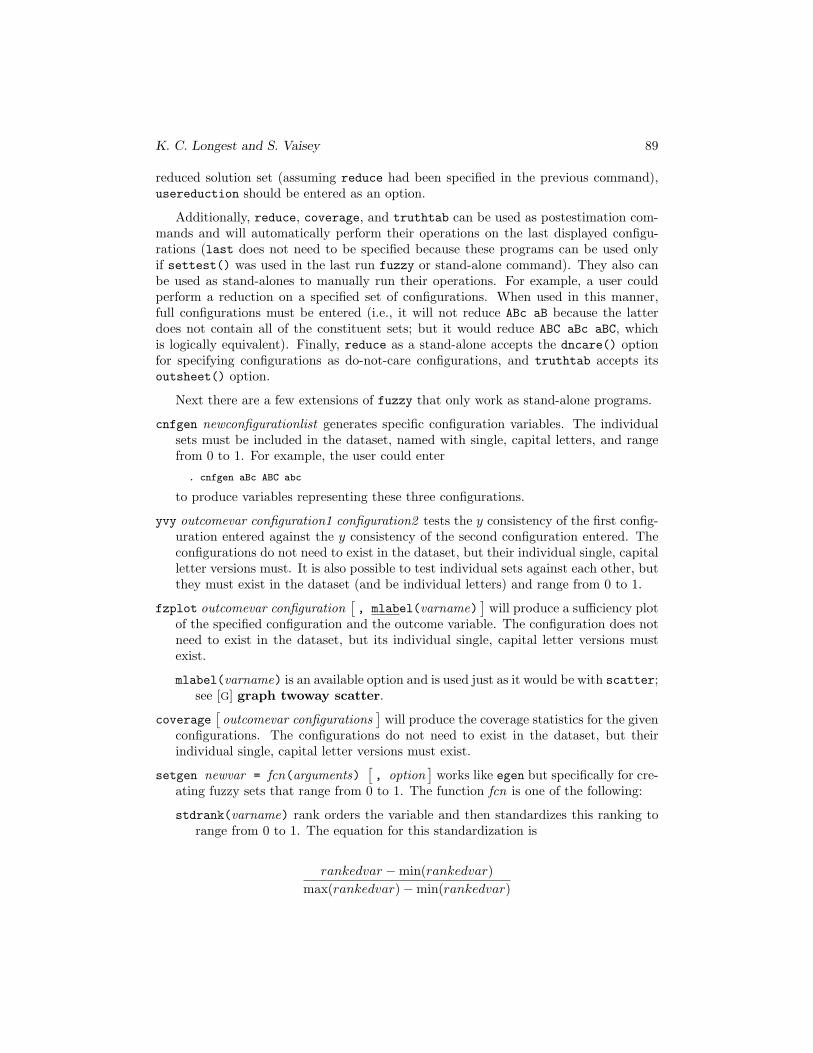
reduced solution set (assuming reduce had been specified in the previous command),usereduction should be entered as an option.

Additionally, reduce, coverage, and truthtab can be used as postestimation com-mands and will automatically perform their operations on the last displayed configu-rations (last does not need to be specified because these programs can be used onlyif settest() was used in the last run fuzzy or stand-alone command). They also canbe used as stand-alones to manually run their operations. For example, a user couldperform a reduction on a specified set of configurations. When used in this manner,full configurations must be entered (i.e., it will not reduce ABc aB because the latterdoes not contain all of the constituent sets; but it would reduce ABC aBc aBC, whichis logically equivalent). Finally, reduce as a stand-alone accepts the dncare() optionfor specifying configurations as do-not-care configurations, and truthtab accepts itsoutsheet() option.

Next there are a few extensions of fuzzy that only work as stand-alone programs.

cnfgen newconfigurationlist generates specific configuration variables. The individualsets must be included in the dataset, named with single, capital letters, and rangefrom 0 to 1. For example, the user could enter

. cnfgen aBc ABC abc

to produce variables representing these three configurations.

yvy outcomevar configuration1 configuration2 tests the y consistency of the first config-uration entered against the y consistency of the second configuration entered. Theconfigurations do not need to exist in the dataset, but their individual single, capitalletter versions must. It is also possible to test individual sets against each other, butthey must exist in the dataset (and be individual letters) and range from 0 to 1.

fzplot outcomevar configuration[, mlabel(varname)

]will produce a sufficiency plot

of the specified configuration and the outcome variable. The configuration does notneed to exist in the dataset, but its individual single, capital letter versions mustexist.

mlabel(varname) is an available option and is used just as it would be with scatter;see [G] graph twoway scatter.

coverage[outcomevar configurations

]will produce the coverage statistics for the given

configurations. The configurations do not need to exist in the dataset, but theirindividual single, capital letter versions must exist.

setgen newvar = fcn(arguments)[, option

]works like egen but specifically for cre-

ating fuzzy sets that range from 0 to 1. The function fcn is one of the following:

stdrank(varname) rank orders the variable and then standardizes this ranking torange from 0 to 1. The equation for this standardization is

rankedvar − min(rankedvar)max(rankedvar) − min(rankedvar)


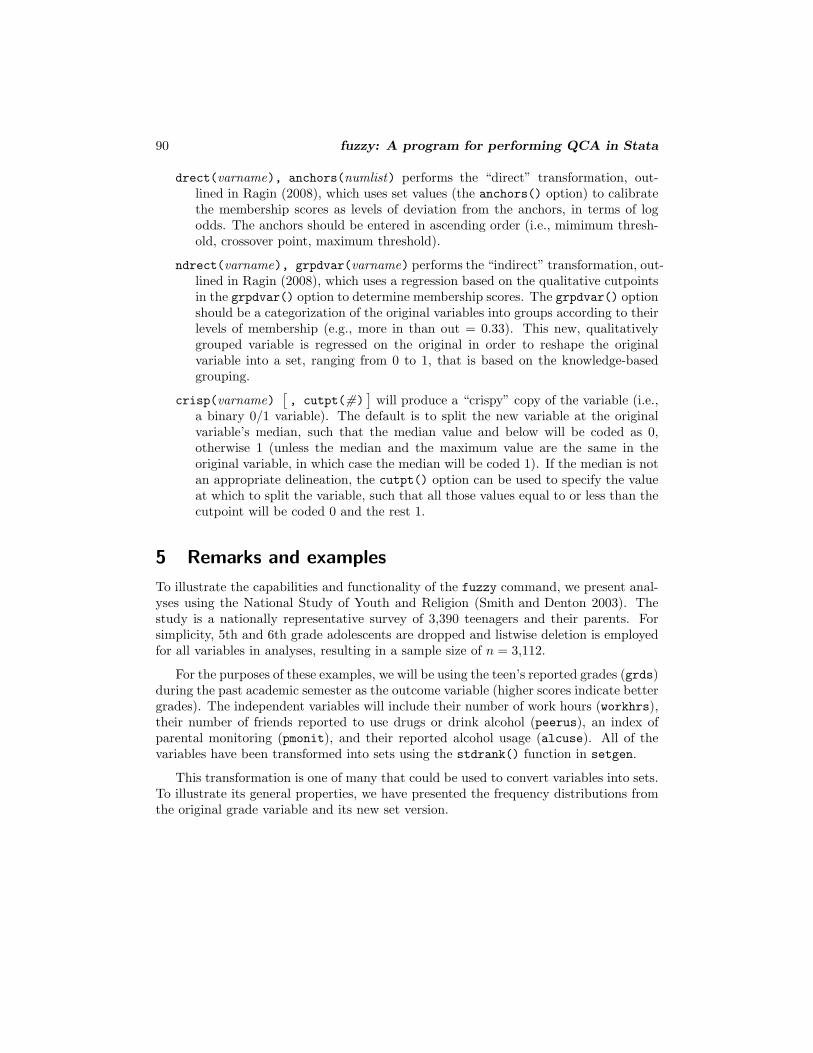
drect(varname), anchors(numlist) performs the “direct” transformation, out-lined in Ragin (2008), which uses set values (the anchors() option) to calibratethe membership scores as levels of deviation from the anchors, in terms of logodds. The anchors should be entered in ascending order (i.e., mimimum thresh-old, crossover point, maximum threshold).

ndrect(varname), grpdvar(varname) performs the “indirect” transformation, out-lined in Ragin (2008), which uses a regression based on the qualitative cutpointsin the grpdvar() option to determine membership scores. The grpdvar() optionshould be a categorization of the original variables into groups according to theirlevels of membership (e.g., more in than out = 0.33). This new, qualitativelygrouped variable is regressed on the original in order to reshape the originalvariable into a set, ranging from 0 to 1, that is based on the knowledge-basedgrouping.

crisp(varname)[, cutpt(#)

]will produce a “crispy” copy of the variable (i.e.,

a binary 0/1 variable). The default is to split the new variable at the originalvariable’s median, such that the median value and below will be coded as 0,otherwise 1 (unless the median and the maximum value are the same in theoriginal variable, in which case the median will be coded 1). If the median is notan appropriate delineation, the cutpt() option can be used to specify the valueat which to split the variable, such that all those values equal to or less than thecutpoint will be coded 0 and the rest 1.

5 Remarks and examples

To illustrate the capabilities and functionality of the fuzzy command, we present anal-yses using the National Study of Youth and Religion (Smith and Denton 2003). Thestudy is a nationally representative survey of 3,390 teenagers and their parents. Forsimplicity, 5th and 6th grade adolescents are dropped and listwise deletion is employedfor all variables in analyses, resulting in a sample size of n = 3,112.

For the purposes of these examples, we will be using the teen’s reported grades (grds)during the past academic semester as the outcome variable (higher scores indicate bettergrades). The independent variables will include their number of work hours (workhrs),their number of friends reported to use drugs or drink alcohol (peerus), an index ofparental monitoring (pmonit), and their reported alcohol usage (alcuse). All of thevariables have been transformed into sets using the stdrank() function in setgen.

This transformation is one of many that could be used to convert variables into sets.To illustrate its general properties, we have presented the frequency distributions fromthe original grade variable and its new set version.


. use nsyr_example_data

. tabulate grds, nol

grds Freq. Percent Cum.

1 13 0.42 0.422 11 0.35 0.773 19 0.61 1.384 88 2.83 4.215 387 12.44 16.656 503 16.16 32.817 402 12.92 45.738 1,088 34.96 80.699 325 10.44 91.1310 276 8.87 100.00

Total 3,112 100.00

. setgen G = stdrank(grds)

. tabulate G

rank of(grds) Freq. Percent Cum.

0 13 0.42 0.42.0040438 11 0.35 0.77.0090986 19 0.61 1.38.0271272 88 2.83 4.21.1071609 387 12.44 16.65.2571188 503 16.16 32.81.409604 402 12.92 45.73.6606571 1,088 34.96 80.69.8987363 325 10.44 91.13

1 276 8.87 100.00

Total 3,112 100.00

The distribution of cases has not changed, but the scale has been “fuzzified” torange between 0 and 1, with the values now representing the level of membership inthe set “good grades”. The similarity of distributions is not required, and in fact thereare situations that may call for more user-knowledge-based coding (for a discussion ofthis type of transformation, see Ragin [2000]). In the current example, we have chosento use the standardized rank transformation because it is a relatively straightforwardconversion.

The following is the distribution of each variable and its corresponding set:

Variable Original range Original mean Set mean

Grades 1–10 7.26 0.52Work hours 0–40 3.31 0.19Peer substance use 0–5 0.70 0.25Parent monitoring 0–4 2.62 0.51Alcohol use 0–5.5 0.60 0.27


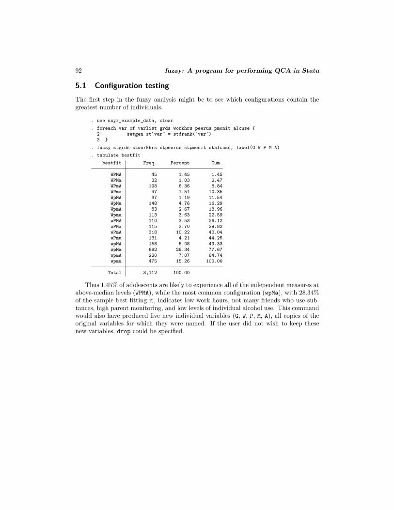
5.1 Configuration testing

The first step in the fuzzy analysis might be to see which configurations contain thegreatest number of individuals.

. use nsyr_example_data, clear

. foreach var of varlist grds workhrs peerus pmonit alcuse {2. setgen st`var´ = stdrank(`var´)3. }

. fuzzy stgrds stworkhrs stpeerus stpmonit stalcuse, label(G W P M A)

. tabulate bestfit

bestfit Freq. Percent Cum.

WPMA 45 1.45 1.45WPMa 32 1.03 2.47WPmA 198 6.36 8.84WPma 47 1.51 10.35WpMA 37 1.19 11.54WpMa 148 4.76 16.29WpmA 83 2.67 18.96Wpma 113 3.63 22.59wPMA 110 3.53 26.12wPMa 115 3.70 29.82wPmA 318 10.22 40.04wPma 131 4.21 44.25wpMA 158 5.08 49.33wpMa 882 28.34 77.67wpmA 220 7.07 84.74wpma 475 15.26 100.00

Total 3,112 100.00

Thus 1.45% of adolescents are likely to experience all of the independent measures atabove-median levels (WPMA), while the most common configuration (wpMa), with 28.34%of the sample best fitting it, indicates low work hours, not many friends who use sub-tances, high parent monitoring, and low levels of individual alcohol use. This commandwould also have produced five new individual variables (G, W, P, M, A), all copies of theoriginal variables for which they were named. If the user did not wish to keep thesenew variables, drop could be specified.


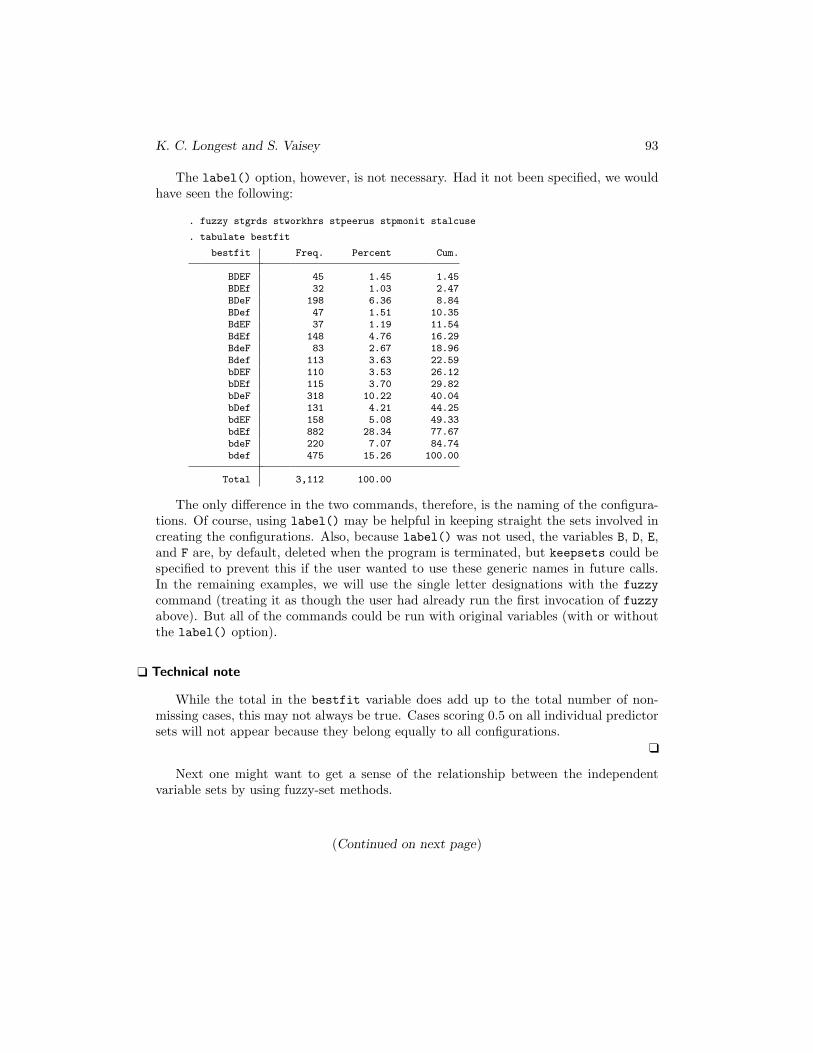
The label() option, however, is not necessary. Had it not been specified, we wouldhave seen the following:

. fuzzy stgrds stworkhrs stpeerus stpmonit stalcuse

. tabulate bestfit

bestfit Freq. Percent Cum.

BDEF 45 1.45 1.45BDEf 32 1.03 2.47BDeF 198 6.36 8.84BDef 47 1.51 10.35BdEF 37 1.19 11.54BdEf 148 4.76 16.29BdeF 83 2.67 18.96Bdef 113 3.63 22.59bDEF 110 3.53 26.12bDEf 115 3.70 29.82bDeF 318 10.22 40.04bDef 131 4.21 44.25bdEF 158 5.08 49.33bdEf 882 28.34 77.67bdeF 220 7.07 84.74bdef 475 15.26 100.00

Total 3,112 100.00

The only difference in the two commands, therefore, is the naming of the configura-tions. Of course, using label() may be helpful in keeping straight the sets involved increating the configurations. Also, because label() was not used, the variables B, D, E,and F are, by default, deleted when the program is terminated, but keepsets could bespecified to prevent this if the user wanted to use these generic names in future calls.In the remaining examples, we will use the single letter designations with the fuzzycommand (treating it as though the user had already run the first invocation of fuzzyabove). But all of the commands could be run with original variables (with or withoutthe label() option).

❑ Technical note

While the total in the bestfit variable does add up to the total number of non-missing cases, this may not always be true. Cases scoring 0.5 on all individual predictorsets will not appear because they belong equally to all configurations.

❑

Next one might want to get a sense of the relationship between the independentvariable sets by using fuzzy-set methods.

(Continued on next page)


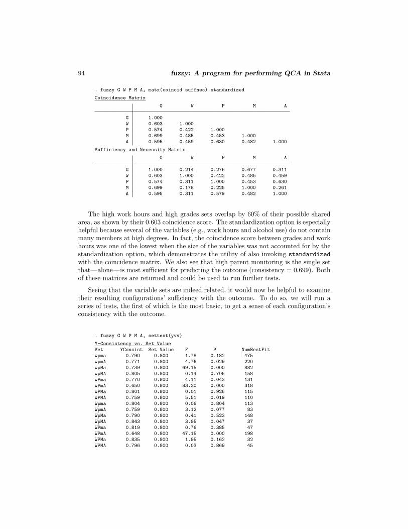
. fuzzy G W P M A, matx(coincid suffnec) standardized

Coincidence Matrix

G W P M A

G 1.000W 0.603 1.000P 0.574 0.422 1.000M 0.699 0.485 0.453 1.000A 0.595 0.459 0.630 0.482 1.000

Sufficiency and Necessity Matrix

G W P M A

G 1.000 0.214 0.276 0.677 0.311W 0.603 1.000 0.422 0.485 0.459P 0.574 0.311 1.000 0.453 0.630M 0.699 0.178 0.225 1.000 0.261A 0.595 0.311 0.579 0.482 1.000

The high work hours and high grades sets overlap by 60% of their possible sharedarea, as shown by their 0.603 coincidence score. The standardization option is especiallyhelpful because several of the variables (e.g., work hours and alcohol use) do not containmany members at high degrees. In fact, the coincidence score between grades and workhours was one of the lowest when the size of the variables was not accounted for by thestandardization option, which demonstrates the utility of also invoking standardizedwith the coincidence matrix. We also see that high parent monitoring is the single setthat—alone—is most sufficient for predicting the outcome (consistency = 0.699). Bothof these matrices are returned and could be used to run further tests.

Seeing that the variable sets are indeed related, it would now be helpful to examinetheir resulting configurations’ sufficiency with the outcome. To do so, we will run aseries of tests, the first of which is the most basic, to get a sense of each configuration’sconsistency with the outcome.

. fuzzy G W P M A, settest(yvv)

Y-Consistency vs. Set ValueSet YConsist Set Value F P NumBestFitwpma 0.790 0.800 1.78 0.182 475wpmA 0.771 0.800 4.76 0.029 220wpMa 0.739 0.800 69.15 0.000 882wpMA 0.805 0.800 0.14 0.705 158wPma 0.770 0.800 4.11 0.043 131wPmA 0.650 0.800 83.20 0.000 318wPMa 0.801 0.800 0.01 0.926 115wPMA 0.759 0.800 5.51 0.019 110Wpma 0.804 0.800 0.06 0.804 113WpmA 0.759 0.800 3.12 0.077 83WpMa 0.790 0.800 0.41 0.523 148WpMA 0.843 0.800 3.95 0.047 37WPma 0.819 0.800 0.76 0.385 47WPmA 0.648 0.800 47.15 0.000 198WPMa 0.835 0.800 1.95 0.162 32WPMA 0.796 0.800 0.03 0.869 45


Each configuration’s consistency is displayed, as well as the resulting test against0.800. The results indicate that only the configuration WpMA is significantly more consis-tent than 0.800 at the 0.05 level. Of course, one of the primary advantages of the fuzzycommand is that it can perform more stringent tests of each configuration’s consistencyvalue. We look for the configurations that have y consistencies significantly greater than0.700, as well as significantly greater than their n consistencies.

. fuzzy G W P M A, settest(yvv yvn) sigonly greater(col1) conval(.700) common

Y-CONSISTENCY vs N-CONSISTENCYSet YCons NCons F P NumBestFitwpma 0.790 0.734 16.49 0.000 475wpMa 0.739 0.646 45.83 0.000 882Wpma 0.804 0.727 6.79 0.009 113WpMa 0.790 0.698 9.46 0.002 148WPma 0.819 0.715 5.70 0.017 47

Y-Consistency vs. Set ValueSet YConsist Set Value F P NumBestFitwpma 0.790 0.700 136.51 0.000 475wpmA 0.771 0.700 27.69 0.000 220wpMa 0.739 0.700 27.20 0.000 882wpMA 0.805 0.700 68.45 0.000 158wPma 0.770 0.700 21.90 0.000 131wPMa 0.801 0.700 48.95 0.000 115wPMA 0.759 0.700 11.33 0.001 110Wpma 0.804 0.700 43.85 0.000 113WpmA 0.759 0.700 6.45 0.011 83WpMa 0.790 0.700 31.27 0.000 148WpMA 0.843 0.700 43.19 0.000 37WPma 0.819 0.700 29.96 0.000 47WPMa 0.835 0.700 28.48 0.000 32WPMA 0.796 0.700 12.50 0.000 45

Common Setswpma wpMa Wpma WpMa WPma

Notice that the sigonly and greater() options apply to both the yvv and yvntests, while conval() pertains only to yvv. Using the common option is a quick wayto see the configurations that pass both tests. From the given output, it appears thatwpma, wpMa, Wpma, WpMa, and WPma are the most highly consistent configurations withgood grades. It is possible though that these configurations may logically overlap. Toperform the reduction:



. fuzzy G W P M A, settest(yvv yvn) sigonly greater(col1) conval(.700)> common reduce

(output omitted )


5 Solutions Entered as True

Minimum Configuration Reduction SetWma pa

Final Reduction Set

CoverageSet Raw Coverage Unique Coverage Solution ConsistencyW*m*a 0.113 0.017 0.778p*a 0.732 0.636 0.603

Total Coverage = 0.749Solution Consistency = 0.604

The five initial configurations have been collapsed into two. (The “Minimum Con-figuration Reduction Set” displays the reduced configurations from the initial step.In certain cases, this will be different than the “Final Reduction Set”, which resultsfrom the second step—employing prime implicants—of the Quine–McCluskey algo-rithm.) We also can tell that low personal alcohol use (a) is key to higher grades.When this base set is conjoined with either low peer substance use (p) or high workhours combined with low parent monitoring (W * m), the adolescent is also likely tobe achieving higher grades.3 Additionally, this example displays the benefit of fuzzymethods more generally, as we find a somewhat surprising relationship between workhours and a positive outcome. Normally, higher work hours have been found to in-crease the likelihood of a number of delinquent activities (Bachman and Schulenberg1993; Safron, Schulenberg, and Bachman 2001; and Paschall, Ringwalt, and Flewelling2002). When this high work intensity, however, is concurrently combined with lowpersonal alcohol use and low parent monitoring, it is associated with higher academicachievement. Understanding why low parent monitoring is included in this configura-tion is difficult without further examination although it may indicate independent youth(i.e., working many hours breaks them from parent monitoring, but they still do notparticipate in delinquent activities, which all conjoins to be associated with positiveacademic outcomes).

Finally, it would have been possible to run the entire set of analyses in the followingsingle command:

3. We recognize that the reduced configuration p*a has a consistency below the 0.7 set value. This dropin value (i.e., increased coverage but reduced effectiveness) is due to the increased amount of people whobelong to the minimized configuration. We recognize this difference as an important methodological(and substantive) issue that should be addressed in future research.


. drop G W P M A

. fuzzy stgrds stworkhrs stpeerus stpmonit stalcuse, label(G W P M A)> matx(coincid suffnec) standard settest(yvv yvn) sigonly greater(col1)> conval(.700) common reduce

(output omitted )



Minimum Configuration Reduction SetWma pa

Final Reduction Set

CoverageSet Raw Coverage Unique Coverage Solution ConsistencySTWORKHRS*stpmonit*stalcuse 0.113 0.017 0.778stpeerus*stalcuse 0.732 0.636 0.603


When the original variables are used along with reduce, the reduction output usesthe original variable names, making it possible to use this output in potential tables.

❑ Technical note

It is possible to pass configurations to that have consistency scores that are greaterwith the negation (i.e., 1 − outcome) than the outcome to reduce (e.g., fuzzy varlist,settest(yvn) greater(col2) reduce), but if this is done, reduce still uses the out-come to compute the coverage and consistency scores of the reduced configurations.If these values are desired for the negation, we suggest the user create a specific vari-able, to be used as the outcome, that represents 1 − outcome and revert to specifyinggreater(col1) with the yvn test.

❑

5.2 Postestimation testing and stand-alones

Many of the options within fuzzy have been constructed to be used as stand-aloneprograms, which may be highly useful to test specific configurations. For example,perhaps one is interested in the coincidence of the configurations, in addition to theindividual variables:



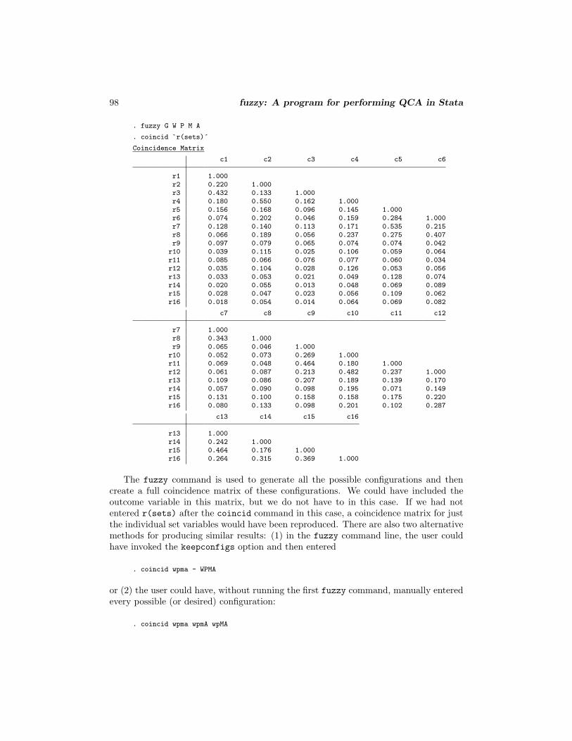
. fuzzy G W P M A

. coincid `r(sets)´

Coincidence Matrix

c1 c2 c3 c4 c5 c6

r1 1.000r2 0.220 1.000r3 0.432 0.133 1.000r4 0.180 0.550 0.162 1.000r5 0.156 0.168 0.096 0.145 1.000r6 0.074 0.202 0.046 0.159 0.284 1.000r7 0.128 0.140 0.113 0.171 0.535 0.215r8 0.066 0.189 0.056 0.237 0.275 0.407r9 0.097 0.079 0.065 0.074 0.074 0.042r10 0.039 0.115 0.025 0.106 0.059 0.064r11 0.085 0.066 0.076 0.077 0.060 0.034r12 0.035 0.104 0.028 0.126 0.053 0.056r13 0.033 0.053 0.021 0.049 0.128 0.074r14 0.020 0.055 0.013 0.048 0.069 0.089r15 0.028 0.047 0.023 0.056 0.109 0.062r16 0.018 0.054 0.014 0.064 0.069 0.082

c7 c8 c9 c10 c11 c12

r7 1.000r8 0.343 1.000r9 0.065 0.046 1.000r10 0.052 0.073 0.269 1.000r11 0.069 0.048 0.464 0.180 1.000r12 0.061 0.087 0.213 0.482 0.237 1.000r13 0.109 0.086 0.207 0.189 0.139 0.170r14 0.057 0.090 0.098 0.195 0.071 0.149r15 0.131 0.100 0.158 0.158 0.175 0.220r16 0.080 0.133 0.098 0.201 0.102 0.287

c13 c14 c15 c16

r13 1.000r14 0.242 1.000r15 0.464 0.176 1.000r16 0.264 0.315 0.369 1.000

The fuzzy command is used to generate all the possible configurations and thencreate a full coincidence matrix of these configurations. We could have included theoutcome variable in this matrix, but we do not have to in this case. If we had notentered r(sets) after the coincid command in this case, a coincidence matrix for justthe individual set variables would have been reproduced. There are also two alternativemethods for producing similar results: (1) in the fuzzy command line, the user couldhave invoked the keepconfigs option and then entered

. coincid wpma - WPMA

or (2) the user could have, without running the first fuzzy command, manually enteredevery possible (or desired) configuration:

. coincid wpma wpmA wpMA


Again, when these postestimation commands are used, only the individual sets(named as capital letters) must exist in the dataset. For example, we could run thefollowing command as long as the set variables G, W, P, M, and A existed in the dataset(even if the configuration variables did not):

. yvn G wpma Wpma WPma

Y-CONSISTENCY vs N-CONSISTENCYSet YCons NCons F P NumBestFitwpma 0.790 0.734 16.49 0.000 475Wpma 0.804 0.727 6.79 0.009 113WPma 0.819 0.715 5.70 0.017 47

When using the options as primary programs, they will accept all of the options as-sociated with them in the main fuzzy (e.g., we could have specified sigonly, slevel(),greater(), or a combination of these in the above example). When using the tests inthis manner, it is still necessary to specify the dependent variable in addition to theconfigurations to be tested.

❑ Technical note

If yvo or cmvom is used in this manner, the “other” configuration that each config-uration is tested against consists only of those configurations that are entered into thecommand line. For example, had yvo been used instead of yvn in the last example, eachconfiguration would have been tested against the other two configurations instead ofthe full possible configuration set. Additionally, if yvo or cmvom is used in this manner,at least two configurations must be specified.

❑



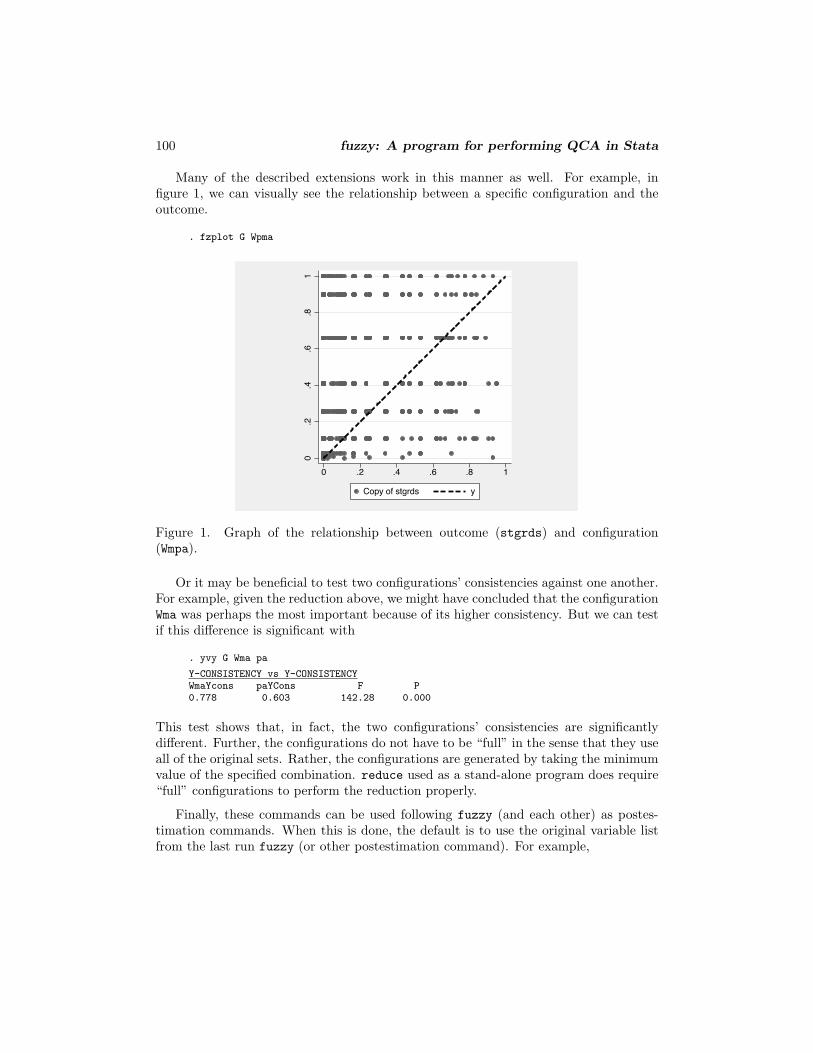
Many of the described extensions work in this manner as well. For example, infigure 1, we can visually see the relationship between a specific configuration and theoutcome.

. fzplot G Wpma

0.2

.4.6

.81

0 .2 .4 .6 .8 1

Copy of stgrds y

Figure 1. Graph of the relationship between outcome (stgrds) and configuration(Wmpa).

Or it may be beneficial to test two configurations’ consistencies against one another.For example, given the reduction above, we might have concluded that the configurationWma was perhaps the most important because of its higher consistency. But we can testif this difference is significant with

. yvy G Wma pa

Y-CONSISTENCY vs Y-CONSISTENCYWmaYcons paYCons F P0.778 0.603 142.28 0.000

This test shows that, in fact, the two configurations’ consistencies are significantlydifferent. Further, the configurations do not have to be “full” in the sense that they useall of the original sets. Rather, the configurations are generated by taking the minimumvalue of the specified combination. reduce used as a stand-alone program does require“full” configurations to perform the reduction properly.

Finally, these commands can be used following fuzzy (and each other) as postes-timation commands. When this is done, the default is to use the original variable listfrom the last run fuzzy (or other postestimation command). For example,


. fuzzy G W P M A

. yvv

Y-Consistency vs. Set ValueSet YConsist Set Value F P NumBestFitwpma 0.790 0.800 1.78 0.182 475wpmA 0.771 0.800 4.76 0.029 220wpMa 0.739 0.800 69.15 0.000 882wpMA 0.805 0.800 0.14 0.705 158wPma 0.770 0.800 4.11 0.043 131wPmA 0.650 0.800 83.20 0.000 318wPMa 0.801 0.800 0.01 0.926 115wPMA 0.759 0.800 5.51 0.019 110Wpma 0.804 0.800 0.06 0.804 113WpmA 0.759 0.800 3.12 0.077 83WpMa 0.790 0.800 0.41 0.523 148WpMA 0.843 0.800 3.95 0.047 37WPma 0.819 0.800 0.76 0.385 47WPmA 0.648 0.800 47.15 0.000 198WPMa 0.835 0.800 1.95 0.162 32WPMA 0.796 0.800 0.03 0.869 45

This is similar to running the command on one line. But it is also possible to run posthoc examination of limited sets of configurations. For example, if in the last run fuzzycommand the display was altered using one of the settest() options or reduce, thenit is possible to specify last or usereduction as an option with the postestimationcommands to restrict their analyses to the last displayed set of configurations.

. fuzzy G W P M A, settest(yvv yvn) sigonly greater(col1) conval(.700) common> reduce

(output omitted )

. yvv, usered conv(.700)

Y-Consistency vs. Set ValueSet YConsist Set Value F P NumBestFitWma 0.778 0.700 27.39 0.000 160pa 0.603 0.700 233.46 0.000 1618

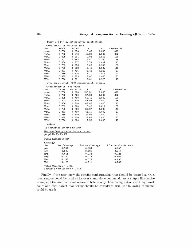
The use of the options as postestimation commands also allows for more complexand flexible sets of tests. For example, if the user wanted to identify and reduce all theconfigurations having consistencies with the outcome that were greater than with thenegation (but not necessarily significantly so) and that were also significantly greaterthan 0.700, it would be impossible to do in one call to fuzzy (because the settest()options apply to all of the tests in settest()). But the user could accomplish this goalusing a simple series of commands:



. fuzzy G W P M A, settest(yvn) greater(col1)

Y-CONSISTENCY vs N-CONSISTENCYSet YCons NCons F P NumBestFitwpma 0.790 0.734 16.49 0.000 475wpMa 0.739 0.646 45.83 0.000 882wpMA 0.805 0.801 0.03 0.855 158wPMa 0.801 0.768 1.50 0.220 115Wpma 0.804 0.727 6.79 0.009 113WpmA 0.759 0.756 0.00 0.949 83WpMa 0.790 0.698 9.46 0.002 148WpMA 0.843 0.796 1.48 0.223 37WPma 0.819 0.715 5.70 0.017 47WPMa 0.835 0.753 3.07 0.080 32WPMA 0.796 0.791 0.01 0.925 45

. yvv, last conval(.700) greater(col1) sigonly

Y-Consistency vs. Set ValueSet YConsist Set Value F P NumBestFitwpma 0.790 0.700 136.51 0.000 475wpMa 0.739 0.700 27.20 0.000 882wpMA 0.805 0.700 68.45 0.000 158wPMa 0.801 0.700 48.95 0.000 115Wpma 0.804 0.700 43.85 0.000 113WpmA 0.759 0.700 6.45 0.011 83WpMa 0.790 0.700 31.27 0.000 148WpMA 0.843 0.700 43.19 0.000 37WPma 0.819 0.700 29.96 0.000 47WPMa 0.835 0.700 28.48 0.000 32WPMA 0.796 0.700 12.50 0.000 45

. reduce


Minimum Configuration Reduction Setpa pM Ma Wp Wa WM

Final Reduction Set

CoverageSet Raw Coverage Unique Coverage Solution Consistencyp*a 0.732 0.134 0.603p*M 0.602 0.026 0.717M*a 0.611 0.034 0.721W*p 0.152 0.013 0.666W*a 0.153 0.012 0.696W*M 0.129 0.011 0.750


Finally, if the user knew the specific configurations that should be treated as true,then reduce could be used as its own stand-alone command. As a simple illustrativeexample, if the user had some reason to believe only those configurations with high workhours and high parent monitoring should be considered true, the following commandcould be used:


. reduce G WpMa WPMa WpMA WPMA


Minimum Configuration Reduction SetWM

Final Reduction Set

CoverageSet Raw Coverage Unique Coverage Solution ConsistencyW*M 0.129 0.129 0.750


As expected, the configuration set reduces to just high work hours (W) and high parentmonitoring (M).

6 Acknowledgments

We would like to thank Nick Cox (University of Durham, UK) for early help with theprogramming that got the larger program off the ground. We also appreciate CharlesRagin and Sarah Strand (University of Arizona) for useful testing and feedback ofearlier versions. The development of this program was supported in part by the Centerfor Developmental Sciences, University of North Carolina at Chapel Hill.

7 ReferencesBachman, J. G., and J. E. Schulenberg. 1993. How part-time work intensity relates to

drug use, problem behavior, time use, and satisfaction among high school seniors: Arethese consequences or merely correlates? Developmental Psychology 29: 220–235.

Greckhamer, T., V. F. Misangyi, H. Elms, and R. Lacey. 2007. Using QualitativeComparative Analysis in Strategic Management Research: An Examination of Com-binations of Industry, Corporate, and Business-unit Effects. Organizational ResearchMethods OnlineFirst 1–32.

Kalleberg, A. L., and S. Vaisey. 2005. Pathways to a good job: Perceived work qualityamong the machinists in North America. British Journal of Industrial Relations 43:431–454.

Lin, N., and W. M. Ensel. 1989. Life stress and health: Stressors and resources. Amer-ican Sociological Review 54: 382–399.

Longest, K. C., and P. Thoits. 2007. The stress process and physical health: A config-urational approach. Paper presented at the American Sociological Annual Meeting.

Mahoney, J. 2003. Long-run development and the legacy of colonialism in SpanishAmerica. American Journal of Sociology 109: 50–106.


Paschall, M. J., C. Ringwalt, and R. L. Flewelling. 2002. Explaining higher levels of al-cohol use among working adolescents: An analysis of potential explanatory variables.Journal of Studies on Alcohol 63: 169–178.

Ragin, C. 2000. Fuzzy-Set Social Science. Chicago: University of Chicago Press.

———. 2006. Set relations in social research: Evaluating the consistency and coverage.Political Analysis 14: 291–310.

———. 2008. Fuzzy set analysis: Calibration versus measurement. In Oxford Handbookof Political Methodology, ed. J. Box-Steffensmeier, H. Brady, and D. Collier. Oxford:Oxford University Press.

Ragin, C. C. 1987. The Comparative Method: Moving Beyond Qualitative and Quan-titative Strategies. Berkeley: University of California Press.

Roscigno, V. J., and R. Hodson. 2004. The organizational and social foundations ofworker resistance. American Sociological Review 69: 14–39.

Safron, D. J., J. E. Schulenberg, and J. G. Bachman. 2001. Part-time work and hurriedadolescence: The links among work intensity, social activities, health behaviors, andsubstance use. Journal of Health and Social Behavior 42: 425–449.

Schuit, A. J., A. J. M. Van Loon, M. Tijhuis, and M. C. Ocke. 2002. Clustering oflifestyle risk factors in a general adult population. Preventive Medicine 35: 219–224.

Shanahan, M. J., L. D. Erikson, S. Vaisey, and A. Smolen. 2007. Helping relationshipsand genetic propensities: A combinatoric study of DRD2, mentoring, and educationalcontinuation. Twin Research and Human Genetics 10: 285–298.

Smith, C., and M. L. Denton. 2003. Methodological design and procedures for theNational Study of Youth and Religion. Technical report, University of North Carolina,Chapel Hill, NC. http://www.youthandreligion.org/.

Smithson, M., and J. Verkuilen. 2006. Fuzzy Set Theory: Applications in the SocialSciences. Thousand Oaks, CA: Sage.

Thoits, P. A. 1995. Stress, coping, and social support processes: Where are we? Whatnext? Journal of Health and Social Behavior 35: 53–79.

Vaisey, S. 2007. Culture, structure, and community: The search for belonging in 50urban communes. American Sociological Review 72: 851–873.

About the authors

Kyle C. Longest is a PhD candidate in the department of sociology at the University of NorthCarolina at Chapel Hill. His research interests focus on adolescent development with specialattention to identity, education, substance use, and the transition out of high school.

Stephen Vaisey is a doctoral student in the department of sociology at the University of NorthCarolina at Chapel Hill. His research focuses on the relationship between culture and cognition.

fuzzy: a program for performing qualitative comparative...

Documents