fundamentals of multilinear subspace learning - sheffieldstaff · fundamentals of multilinear...

Chapter 3

Fundamentals of Multilinear SubspaceLearning

The previous chapter covered background materials on linear subspace learn-ing. From this chapter on, we shall proceed to multiple dimensions with tensor-level computational thinking. Multilinear algebra is the foundation of multi-linear subspace learning (MSL). Thus, we first review the basic notations andoperations in multilinear algebra, as well as popular tensor decompositions.In the presentation, we include some discussions of the second-order case (formatrix data) as well, which can be understood in the context of linear algebra.Next, we introduce the important concept of multilinear projections for directmapping of tensors to a lower-dimensional representation, as shown in Figure3.1. They include elementary multilinear projection (EMP), tensor-to-vectorprojection (TVP), and tensor-to-tensor projection (TTP), which project aninput tensor to a scalar, a vector, and a tensor, respectively. Their relation-ships are analyzed in detail subsequently. Finally, we extend commonly usedvector-based scatter measures to tensors and scalars for optimality criterionconstruction in MSL.

FIGURE 3.1: Multilinear subspace learning finds a lower-dimensional rep-resentation by direct mapping of tensors through a multilinear projection.

49

50 Multilinear Subspace Learning

3.1 Multilinear Algebra Preliminaries

Multilinear algebra, the basis of tensor-based computing, has been studied inmathematics for several decades [Greub, 1967]. A tensor is a multidimensional(multiway) array. As pointed out by Kolda and Bader [2009], this notion oftensors is different from the same term referring to tensor fields in physicsand engineering. In the following, we review the notations and some basicmultilinear operations needed in introducing MSL.

3.1.1 Notations and Definitions

In this book, we have tried to remain consistent with the notations and termi-nologies in applied mathematics, particularly the seminal paper by De Lath-auwer et al. [2000b] and the recent SIAM review paper on tensor decomposi-tion by Kolda and Bader [2009].

Vectors are denoted by lowercase boldface letters, for example, a; matricesby uppercase boldface, for example, A; and tensors by calligraphic letters,for example, A. Indices are denoted by lowercase letters and span the rangefrom 1 to the uppercase letter of the index whenever appropriate, for example,n = 1, 2, ..., N . Throughout this book, we restrict the discussions to real-valuedvectors, matrices, and tensors.

Definition 3.1. The number of dimensions (ways) of a tensor is its order,denoted by N . Each dimension (way) is called a mode.

As shown in Figure 3.2, a scalar is a zero-order tensor (N = 0), a vector isa first-order tensor (N = 1), and a matrix is a second-order tensor (N = 2).Tensors of order three or higher are called higher-order tensors. An Nth-ordertensor is an element in a tensor space of degree N , the tensor product (outerproduct) of N vector spaces (Section A.1.4) [Lang, 1984].

Mode addressing: There are two popular ways to refer to a mode: n-mode or mode-n. In [De Lathauwer et al., 2000b], only n-mode is used. In[De Lathauwer et al., 2000a], n-mode and mode-n are used interchangeably.In [Kolda and Bader, 2009], n-mode and mode-n are used in different contexts.In this book, we prefer to use mode-n to indicate the nth mode for clarity.

FIGURE 3.2: Illustration of tensors of order N = 0, 1, 2, 3, 4.

Fundamentals of Multilinear Subspace Learning 51

For example, “1-mode” (referring to the mode index) may be confused withone mode (referring to the number of modes).

An Nth-order tensor has N indices {in}, n = 1, ..., N , with each indexin(= 1, ..., In) addressing mode-n of A. Thus, we denote an Nth-order tensorexplicitly as A ∈ RI1×I2×...×IN .

When we have a set of N vectors or matrices, one for each mode, we denotethe nth (i.e., mode-n) vector or matrix using a superscript in parenthesis,for example, as u(n) or U(n) and the whole set as {u(1),u(2), ...,u(N)} or{U(1),U(2), ...,U(N)}, or more compactly as {u(n)} or {U(n)}. Figures 3.5,3.9, and 3.10 provide some illustrations.

Element addressing: For clarity, we adopt the MATLAB style to addresselements (entries) of a tensor (including vector and matrix) with indices inparentheses. for example, a single element (entry) is denoted as a(2), A(3, 4),or A(5, 6, 7) in this book, which are denoted as a2, a34, or a567 in conventionalnotations1. To address part of a tensor (a subarray), “:” denotes the full rangeof the corresponding index and i : j denotes indices ranging from i to j, forexample, a(2 : 5), A(3, :) (the third row), or A(1 : 3, :, 4 : 5).

Definition 3.2. The mode-n vectors2 of A are defined as the In-dimensional vectors obtained from A by varying the index in while keepingall the other indices fixed.

For example, A(:, 2, 3) is a mode-1 vector. For second-order tensors (matri-ces), mode-1 and mode-2 vectors are the column and row vectors, respectively.Figures 3.3(b), 3.3(c), and 3.3(d) give visual illustrations of the mode-1, mode-2, and mode-3 vectors of the third-order tensorA in Figure 3.3(a), respectively.

Definition 3.3. The inth mode-n slice of A is defined as an (N−1)th-ordertensor obtained by fixing the mode-n index of A to be in: A(:, ..., :, in, :, ..., :).

For example, A(:, 2, :) is a mode-2 slice of A. For second-order tensors(matrices), a mode-1 slice is a mode-2 (row) vector, and a mode-2 slice is amode-1 (column) vector. Figures 3.4(b), 3.4(c), and 3.4(d) give visual illus-trations of the mode-1, mode-2, and mode-3 slices of the third-order tensor Ain Figure 3.4(a), respectively. This definition of a slice is consistent with thatin [Bader and Kolda, 2006]; however, it is different from the definition of aslice in [Kolda and Bader, 2009], where a slice is defined as a two-dimensionalsection of a tensor.

Definition 3.4. A rank-one tensor A ∈ RI1×I2×...×IN equals the outerproduct3 of N vectors:

A = u(1) ◦ u(2) ◦ ... ◦ u(N), (3.1)

1In Appendix A, we follow the conventional notations of an element.2Mode-n vectors are renamed as mode-n fibers in [Kolda and Bader, 2009].3Here, we use a notation ‘◦’ different from the conventional notation ‘⊗’ to better

differentiate the outer product of vectors from the Kronecker product of matrices.


(a) (b) (c) (d)

FIGURE 3.3: Illustration of the mode-n vectors: (a) a tensor A ∈ R8×6×4,(b) the mode-1 vectors, (c) the mode-2 vectors, and (d) the mode-3 vectors.

(a) (b) (c) (d)

FIGURE 3.4: Illustration of the mode-n slices: (a) a tensor A ∈ R8×6×4, (b)the mode-1 slices, (c) the mode-2 slices, and (d) the mode-3 slices.

which means that

A(i1, i2, ..., iN ) = u(1)(i1) · u(2)(i2) · ... · u(N)(iN ) (3.2)

for all values of indices.

A rank-one tensor for N = 2 (i.e., a second-order rank-one tensor) is arank-one matrix, with an example shown in Figure 3.5. Some examples ofrank-one tensors for N = 2, 3 learned from real data are shown in Figures1.10(c) and 1.11(c) in Chapter 1.

Definition 3.5. A cubical tensor A ∈ RI1×I2×...×IN has the same size forevery mode, that is, In = I for n = 1, ..., N [Kolda and Bader, 2009].

Thus, a square matrix is a second-order cubical tensor by this definition.


FIGURE 3.5: An example of second-order rank-one tensor (that is, rank-one

matrix): A = u(1) ◦ u(2) = u(1)u(2)T .

FIGURE 3.6: The diagonal of a third-order cubical tensor.

Definition 3.6. A diagonal tensor A ∈ RI1×I2×...×IN has non-zero entries,i.e., A(i1, i2, ..., iN ) 6= 0, only for i1 = i2 = ... = iN [Kolda and Bader, 2009].

A diagonal tensor of order 2 (N = 2) is simply a diagonal matrix. Adiagonal tensor of order 3 (N = 3) has non-zero entries only along its diagonalas shown in Figure 3.6. A vector d ∈ RI consisting of the diagonal of a cubicaltensor can be defined as

d = diag(A), where d(i) = A(i, i, ..., i). (3.3)

3.1.2 Basic Operations

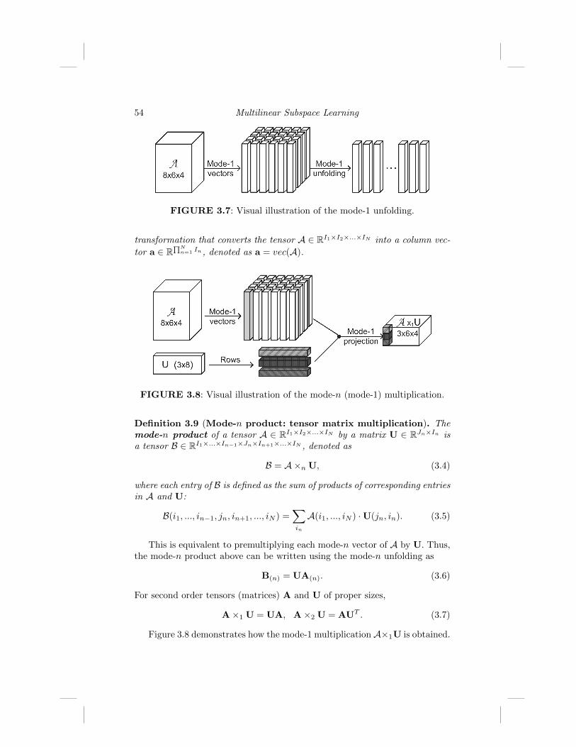
Definition 3.7 (Unfolding: tensor to matrix transformation4). A ten-sor can be unfolded into a matrix by rearranging its mode-n vectors. Themode-n unfolding of A is denoted by A(n) ∈ RIn×(I1×...×In−1×In+1×...×IN ),where the column vectors of A(n) are the mode-n vectors of A.

The (column) order of the mode-n vectors in A(n) is usually not importantas long as it is consistent throughout the computation. For a second-ordertensor (matrix) A, its mode-1 unfolding is itself A and its mode-2 unfoldingis its transpose AT . Figure 3.7 shows the mode-1 unfolding of the third-ordertensor A on the left.

Definition 3.8 (Vectorization: tensor to vector transformation). Sim-ilar to the vectorization of a matrix, the vectorization of a tensor is a linear

4Unfolding is also known as flattening or matricization [Kolda and Bader, 2009].


FIGURE 3.7: Visual illustration of the mode-1 unfolding.

transformation that converts the tensor A ∈ RI1×I2×...×IN into a column vec-

tor a ∈ R∏Nn=1 In , denoted as a = vec(A).

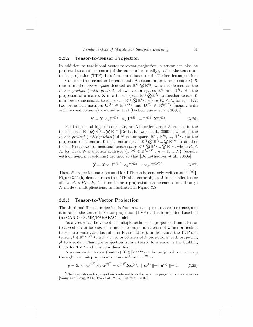
FIGURE 3.8: Visual illustration of the mode-n (mode-1) multiplication.

Definition 3.9 (Mode-n product: tensor matrix multiplication). Themode-n product of a tensor A ∈ RI1×I2×...×IN by a matrix U ∈ RJn×In isa tensor B ∈ RI1×...×In−1×Jn×In+1×...×IN , denoted as

B = A×n U, (3.4)

where each entry of B is defined as the sum of products of corresponding entriesin A and U:

B(i1, ..., in−1, jn, in+1, ..., iN ) =∑in

A(i1, ..., iN ) ·U(jn, in). (3.5)

This is equivalent to premultiplying each mode-n vector of A by U. Thus,the mode-n product above can be written using the mode-n unfolding as

B(n) = UA(n). (3.6)

For second order tensors (matrices) A and U of proper sizes,

A×1 U = UA, A×2 U = AUT . (3.7)

Figure 3.8 demonstrates how the mode-1 multiplicationA×1U is obtained.


The product A×1 U is computed as the inner products between the mode-1vectors of A and the rows of U. In the mode-1 multiplication in Figure 3.8,each mode-1 vector of A (∈ R8) is projected by U ∈ R3×8 to obtain a vector(∈ R3), as the differently shaded vector indicates in the right of the figure.

Tensor matrix multiplication has the following two properties [De Lath-auwer et al., 2000b].

Property 3.1. Given a tensor A ∈ RI1×I2×...×IN , and two matrices U ∈RJn×In and V ∈ RJm×Im , where m 6= n, we have

(A×m U)×n V = (A×n V)×m U. (3.8)

Property 3.2. Given a tensor A ∈ RI1×I2×...×IN , and two matrices U ∈RJn×In and V ∈ RKn×In , we have

(A×n U)×n V = A×n (V ·U). (3.9)

Definition 3.10 (Mode-n product: tensor vector multiplication). Themode-n product of a tensor A ∈ RI1×I2×...×IN by a vector u ∈ RIn×1 is atensor C ∈ RI1×...×In−1×1×In+1×...×IN , denoted as

C = A×n uT , (3.10)

where each entry of C is defined as

C(i1, ..., in−1, 1, in+1, ..., iN ) =∑in

A(i1, ..., iN ) · u(in). (3.11)

Multiplication of a tensor by a vector can be viewed as a special case oftensor matrix multiplication with Jn = 1 (so U ∈ RJn×In = uT ). This productA×1 uT can be computed as the inner products between the mode-1 vectorsof A and u. Note that the nth dimension of C is 1, so effectively the order ofC is reduced to N − 1. The squeeze() function in MATLAB can remove allmodes with dimension equal to one.

Definition 3.11. The scalar product (inner product) of two same-sizedtensors A,B ∈ RI1×I2×...×IN is defined as

< A,B >=∑i1

∑i2

...∑iN

A(i1, i2, ..., iN ) · B(i1, i2, ..., iN ). (3.12)

This can be seen as a generalization of the inner product in linear algebra(Section A.1.4).

Definition 3.12. The Frobenius norm of A is defined as

‖ A ‖F=√< A,A >. (3.13)

This is a straightforward extension of the matrix Frobenius norm (SectionA.1.5).


3.1.3 Tensor/Matrix Distance Measure

The Frobenius norm can be used to measure the distance between tensors Aand B as

dist(A,B) =‖ A − B ‖F . (3.14)

Although this is a tensor-based measure, it is equivalent to a distance measureof corresponding vector representations denoted as vec(A) and vec(B), as tobe shown in the following. We first derive a property regarding the scalarproduct between two tensors:

Proposition 3.1. < A,B >=< vec(A), vec(B) >= [vec(B)]Tvec(A).

Proof. Let a = vec(A) and b = vec(B) for convenience. From Equation (3.12),< A,B > is the summing the products between all corresponding entries inA and B. We can have the same results by the sum of products between allcorresponding entries in a and b, their vectorizations. Thus, we have

< A,B > =

I1∑i1=1

I2∑i2=1

...

IN∑iN=1

A(i1, i2, ..., iN ) · B(i1, i2, ..., iN )

=

∏Nn=1 In∑i=1

a(i) · b(i)

= < a,b >

= [b]T

a.

Then, it is straightforward to show the equivalence.

Proposition 3.2. dist(A,B) =‖ vec(A)− vec(B) ‖2.

Proof. From Proposition 3.1,

dist(A,B) = ‖ A − B ‖F=

√< (A− B), (A− B) >

=√< vec(A)− vec(B), vec(A)− vec(B) >

= ‖ vec(A)− vec(B) ‖2 .

Proposition 3.2 indicates that the Frobenius norm of the difference betweentwo tensors equals the Euclidean distance between their vectorized represen-tations. The tensor Frobenius norm is a point-based measurement [Lu et al.,2004] without taking the tensor structure into account.

For second-order tensors, that is, matrices, their distance can be measured


by the matrix Frobenius norm, which equals the square root of the trace ofthe difference matrix:

dist(A,B) =‖ A−B ‖F=√

tr ((A−B)T (A−B)). (3.15)

An alternative for matrix distance is the so-called volume measure used in[Meng and Zhang, 2007]. The volume measure between matrices A and B isdefined as

dist(A,B) = vol(A−B) =√|(A−B)T (A−B)|, (3.16)

where | · | denotes the determinant.The matrix Frobenius norm is further generalized as the assembled matrix

distance (AMD) in [Zuo et al., 2006] as

dAMD(A,B) =

I1∑i1=1

(I2∑i2=1

(A(i1, i2)−B(i1, i2))2

)p/21/p

, (3.17)

where the power p weights the differences between elements. AMD is a vari-ation of the p-norm for vectors and it treats a matrix as a vector effectively.AMD with p = 2 is equivalent to the matrix Frobenius norm and the Eu-clidean norm for vectors. The AMD measure can be generalized to generalhigher-order tensors, or it can also be modified to take data properties (suchas shape and connectivity) into account as in [Porro-Munoz et al., 2011].

Distance measures are frequently used by classifiers to measure similarityor dissimilarity. Furthermore, it is possible to design classifiers by taking intoaccount the matrix/tensor representation or structure. For example, Wanget al. [2008] proposed a classifier specially designed for matrix representa-tions of patterns and showed that such a classifier has advantages in featuresextracted from matrix representations.

3.2 Tensor Decompositions

Multilinear subspace learning is based on tensor decompositions. This sectionreviews two most important works in this area.

3.2.1 CANDECOMP/PARAFAC

Hitchcock [1927a,b] first proposed the idea of expressing a tensor as thesum of rank-one tensors in polyadic form. It became popular in the psycho-metrics community with the independent introduction of canonical decom-position (CANDECOMP) by Carroll and Chang [1970] and parallel factors(PARAFAC) by Harshman [1970].


FIGURE 3.9: The CANDECOMP/PARAFAC decomposition of a third-order tensor.

FIGURE 3.10: The Tucker decomposition of a third-order tensor.

With the CANDECOMP/PARAFAC decomposition (CP decomposition),a tensor A can be factorized into a linear combination of P rank-one tensors:

A =

P∑p=1

λpu(1)p ◦ u(2)

p ◦ ... ◦ u(N)p , (3.18)

where P ≤∏Nn=1 In. Figure 3.9 illustrates this decomposition.

3.2.2 Tucker Decomposition and HOSVD

The Tucker decomposition [Tucker, 1966] was introduced in the 1960s. It de-composes an Nth-order tensor A into a core tensor S multiplied by N matri-ces, one in each mode:

A = S ×1 U(1) ×2 U(2) × ...×N U(N), (3.19)

where Pn ≤ In for n = 1, ..., N , and U(n) =[u

(n)1 u

(n)2 ...u

(n)Pn

]is an In ×

Pn matrix often assumed to have orthonormal column vectors. Figure 3.10illustrates this decomposition.

The Tucker decomposition was investigated mainly in psychometrics afterits initial introduction. It was reintroduced by De Lathauwer et al. [2000b] asthe higher-order singular value decomposition (HOSVD) to the communitiesof numerical algebra and signal processing, followed by many other disciplines.When Pn = In for n = 1, ..., N and {U(n), n = 1, ..., N} are all orthogonal


In × In matrices, then from Equation (3.19), the core tensor can be writtenas

S = A×1 U(1)T ×2 U(2)T ...×N U(N)T . (3.20)

Because U(n) has orthonormal columns, we have [De Lathauwer et al., 2000a]

‖ A ‖2F=‖ S ‖2F . (3.21)

A matrix representation of this decomposition can be obtained by unfoldingA and S as

A(n) = U(n) · S(n) ·(U(n+1) ⊗ ...⊗U(N) ⊗U(1) ⊗ ...⊗U(n−1)

)T, (3.22)

where ⊗ denotes the Kronecker product (Section A.1.4). The decompositioncan also be written as

A =

I1∑i1=1

I2∑i2=1

...

IN∑iN=1

S(i1, i2, ..., iN )u(1)i1◦ u

(2)i2◦ ... ◦ u

(N)iN

, (3.23)

that is, any tensor A can be written as a linear combination of∏Nn=1 In rank-

one tensors. Comparison of Equation (3.23) against Equation (3.18) revealsthe equivalence between Tucker decomposition and CP decomposition.

3.3 Multilinear Projections

A tensor subspace is defined through a multilinear projection that maps theinput data from a high-dimensional space to a low-dimensional space [Heet al., 2005a]. Therefore, multilinear projection is an important concept tograsp before proceeding to multilinear subspace learning.

This section presents three basic multilinear projections named in terms ofthe input and output representations of the projection: the traditional vector-to-vector projection, the tensor-to-tensor projection, and the tensor-to-vectorprojection. Furthermore, we investigate the relationships among these projec-tions.

3.3.1 Vector-to-Vector Projection

Linear projection is a standard transformation used widely in various applica-tions [Duda et al., 2001; Moon and Stirling, 2000]. A linear projection takes avector x ∈ RI as input and projects it to a vector y ∈ RP using a projectionmatrix U ∈ RI×P :

y = UTx = x×1 UT . (3.24)


(a)

(b)

(c)

FIGURE 3.11: Illustration of (a) vector-to-vector projection, (b) tensor-to-tensor projection, and (c) tensor-to-vector projection, where EMP stands forelementary multilinear projection.

If we name this projection according to its input and output representations,linear projection is a vector-to-vector projection because it maps a vector toanother vector. When the input data is a matrix or a higher-order tensor,it needs to be vectorized (reshaped into a vector) before projection. Figure3.11(a) illustrates the vector-to-vector projection of a tensor object A.

Denote each column of U as up, so U = [u1 u2 ... uP ]. Then each columnup projects x to a scalar y(p) or yp:

yp = y(p) = uTp x. (3.25)


3.3.2 Tensor-to-Tensor Projection

In addition to traditional vector-to-vector projection, a tensor can also beprojected to another tensor (of the same order usually), called the tensor-to-tensor projection (TTP). It is formulated based on the Tucker decomposition.

Consider the second-order case first. A second-order tensor (matrix) Xresides in the tensor space denoted as RI1

⊗RI2 , which is defined as the

tensor product (outer product) of two vector spaces RI1 and RI2 . For theprojection of a matrix X in a tensor space RI1

⊗RI2 to another tensor Y

in a lower-dimensional tensor space RP1⊗

RP2 , where Pn ≤ In for n = 1, 2,two projection matrices U(1) ∈ RI1×P1 and U(2) ∈ RI2×P2 (usually withorthonormal columns) are used so that [De Lathauwer et al., 2000a]

Y = X×1 U(1)T ×2 U(2)T = U(1)TXU(2). (3.26)

For the general higher-order case, an Nth-order tensor X resides in thetensor space RI1

⊗RI2 ...

⊗RIN [De Lathauwer et al., 2000b], which is the

tensor product (outer product) of N vector spaces RI1 , RI2 , ..., RIN . For theprojection of a tensor X in a tensor space RI1

⊗RI2 ...

⊗RIN to another

tensor Y in a lower-dimensional tensor space RP1⊗

RP2 ...⊗

RPN , where Pn ≤In for all n, N projection matrices {U(n) ∈ RIn×Pn , n = 1, ..., N} (usuallywith orthonormal columns) are used so that [De Lathauwer et al., 2000a]

Y = X ×1 U(1)T ×2 U(2)T ...×N U(N)T . (3.27)

These N projection matrices used for TTP can be concisely written as {U(n)}.Figure 3.11(b) demonstrates the TTP of a tensor object A to a smaller tensorof size P1 × P2 × P3. This multilinear projection can be carried out throughN mode-n multiplications, as illustrated in Figure 3.8.

3.3.3 Tensor-to-Vector Projection

The third multilinear projection is from a tensor space to a vector space, andit is called the tensor-to-vector projection (TVP)5. It is formulated based onthe CANDECOMP/PARAFAC model.

As a vector can be viewed as multiple scalars, the projection from a tensorto a vector can be viewed as multiple projections, each of which projects atensor to a scalar, as illustrated in Figure 3.11(c). In the figure, the TVP of atensor A ∈ R8×6×4 to a P ×1 vector consists of P projections, each projectingA to a scalar. Thus, the projection from a tensor to a scalar is the buildingblock for TVP and it is considered first.

A second-order tensor (matrix) X ∈ RI1×I2 can be projected to a scalar ythrough two unit projection vectors u(1) and u(2) as

y = X×1 u(1)T ×2 u(2)T = u(1)TXu(2), ‖ u(1) ‖=‖ u(2) ‖= 1, (3.28)

5The tensor-to-vector projection is referred to as the rank-one projections in some works[Wang and Gong, 2006; Tao et al., 2006; Hua et al., 2007].


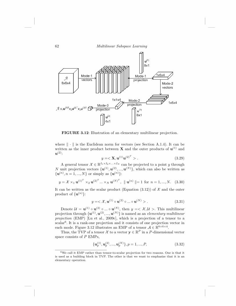
FIGURE 3.12: Illustration of an elementary multilinear projection.

where ‖ · ‖ is the Euclidean norm for vectors (see Section A.1.4). It can bewritten as the inner product between X and the outer products of u(1) andu(2):

y =< X,u(1)u(2)T > . (3.29)

A general tensor X ∈ RI1×I2×...×IN can be projected to a point y throughN unit projection vectors {u(1),u(2), ...,u(N)}, which can also be written as{u(n), n = 1, ..., N} or simply as {u(n)}:

y = X ×1 u(1)T ×2 u(2)T ...×N u(N)T , ‖ u(n) ‖= 1 for n = 1, ..., N. (3.30)

It can be written as the scalar product (Equation (3.12)) of X and the outerproduct of {u(n)}:

y =< X ,u(1) ◦ u(2) ◦ ... ◦ u(N) > . (3.31)

Denote U = u(1) ◦ u(2) ◦ ... ◦ u(N), then y =< X ,U >. This multilinearprojection through {u(1),u(2), ...,u(N)} is named as an elementary multilinearprojection (EMP) [Lu et al., 2009c], which is a projection of a tensor to ascalar6. It is a rank-one projection and it consists of one projection vector ineach mode. Figure 3.12 illustrates an EMP of a tensor A ∈ R8×6×4.

Thus, the TVP of a tensor X to a vector y ∈ RP in a P -dimensional vectorspace consists of P EMPs,

{u(1)p ,u(2)

p , ...,u(N)p }, p = 1, ..., P, (3.32)

6We call it EMP rather than tensor-to-scalar projection for two reasons. One is that itis used as a building block in TVP. The other is that we want to emphasize that it is anelementary operation.


which can be written concisely as {u(n)p , n = 1, ..., N}Pp=1 or simply as {u(n)

p }PN .The TVP from X to y is then written as

y = X ×Nn=1 {u(n)p , n = 1, ..., N}Pp=1 = X ×Nn=1 {u(n)

p }PN , (3.33)

where the pth entry of y is obtained from the pth EMP as

yp = y(p) = X ×1 u(1)T

p ×2 u(2)T

p ...×N u(N)T

p = X ×Nn=1 {u(n)p }. (3.34)

Figure 3.11(c) shows the TVP of a tensor A to a vector of size P × 1.

3.4 Relationships among Multilinear Projections

With the introduction of the three basic multilinear projections, it is worth-while to investigate their relationships.

Degenerated conditions: It is easy to verify that the vector-to-vectorprojection is the special case of the tensor-to-tensor projection and the tensor-to-vector projection for N = 1. The elementary multilinear projection is thedegenerated version of the tensor-to-tensor projection with Pn = 1 for all n.

EMP view of TTP: Each projected element in the tensor-to-tensor pro-jection can be viewed as the projection by an elementary multilinear pro-jection formed by taking one column from each modewise projection matrix.Thus, a projected tensor in the tensor-to-tensor projection is obtained through∏Nn=1 Pn elementary multilinear projections with shared projection vectors

(from the projection matrices) in effect, while in the tensor-to-vector projec-tion, the P elementary multilinear projections do not have shared projectionvectors.

Equivalence between EMP and VVP: Recall that the projection usingan elementary multilinear projection {u(1),u(2), ...,u(N)} can be written as

y =< X ,U >=< vec(X ), vec(U) >= [vec(U)]Tvec(X ), (3.35)

by Proposition 3.1. Thus, an elementary multilinear projection is equivalent toa linear projection of vec(X ), the vectorized representation of X , by a vectorvec(U) as in Equation (3.25). Because U = u(1) ◦ u(2) ◦ ... ◦ u(N), Equation(3.35) indicates that the elementary multilinear projection is equivalent to alinear projection for P = 1 with a constraint on the projection vector suchthat it is the vectorized representation of a rank-one tensor.

Equivalence between TTP and TVP: Given a TVP {u(n)p }PN , we can

form N matrices {V(n)}, where

V(n) = [u(n)1 , ...,u(n)

p , ...,u(n)P ] ∈ RIn×P . (3.36)

These matrices can be viewed as a TTP with Pn = P for n = 1, ..., N (equal


subspace dimensions in all modes). Thus, the TVP of a tensor by {u(n)p }PN

is equivalent to the diagonal of a corresponding TTP of the same tensor by{V(n)} as defined in Equation (3.36):

y = X ×Nn=1 {u(n)p }PN (3.37)

= diag(X ×1 V(1)T ×2 V(2)T ...×N V(N)T

). (3.38)

In the second-order case, this equivalence is

y = diag(V(1)TXV(2)

). (3.39)

Number of parameters to estimate: The number of parameters to beestimated in a particular projection indicates model complexity, an impor-tant concern in practice. Compared with a projection vector of size I × 1 ina VVP specified by I parameters (I =

∏Nn=1 In for an Nth-order tensor),

an EMP in a TVP is specified by∑Nn=1 In parameters. Hence, to project a

tensor of size∏Nn=1 In to a vector of size P × 1, TVP needs to estimate only

P ·∑Nn=1 In parameters, while VVP needs to estimate P ·

∏Nn=1 In param-

eters. The implication is that TVP has fewer parameters to estimate whilebeing more constrained on the solutions, and VVP has less constraint on thesolutions sought while having more parameters to estimate. In other words,TVP has a simpler model than VVP. For TTP with the same amount of di-mensionality reduction

∏Nn=1 Pn = P ,

∑Nn=1 Pn × In parameters need to be

estimated. Thus, due to shared projection vectors, TTP may need to estimateeven fewer parameters and its model can be even simpler.

Table 3.1 contrasts the number of parameters to be estimated by the threeprojections for the same amount of dimensionality reduction for several cases.Figure 3.13 further illustrates the first three cases, where the numbers of pa-rameters are normalized with respect to that by VVP for better visualization.From the table and figure, we can see that for higher-order tensors, the con-ventional VVP model becomes extremely complex and parameter estimationbecomes extremely difficult. This often leads to the small sample size (SSS)problem in practice when there are limited number of training samples avail-able.

3.5 Scatter Measures for Tensors and Scalars

3.5.1 Tensor-Based Scatters

In analogy to the definitions of scatters in Equations (2.1), (2.27), and (2.25)for vectors used in linear subspace learning, we define tensor-based scattersto be used in multilinear subspace learning (MSL) through TTP.


TABLE 3.1: Number of parameters to be estimated by three multilinearprojections.

Input Output VVP TVP TTP∏Nn=1 In P P ·

∏Nn=1 In P ·

∑Nn=1 In

∑Nn=1 Pn × In

10× 10 4 400 80 40 (Pn = 2)

100× 100 4 40,000 800 400 (Pn = 2)

100× 100× 100 8 8,000,000 2,400 600 (Pn = 2)∏4n=1 100 16 1,600,000,000 6,400 800 (Pn = 2)

FIGURE 3.13: Comparison of the number of parameters to be estimatedby VVP, TVP, and TTP, normalized with respect to the number by VVP forvisualization.

Definition 3.13. Let {Am,m = 1, ...,M} be a set of M tensor samples inRI1

⊗RI2 ...

⊗RIN . The total scatter of these tensors is defined as

ΨTA =

M∑m=1

‖ Am − A ‖2F , (3.40)

where A is the mean tensor calculated as

A =1

M

M∑m=1

Am. (3.41)

The mode-n total scatter matrix of these samples is then defined as

S(n)TA

=M∑m=1

(Am(n) − A(n)

) (Am(n) − A(n)

)T, (3.42)


where Am(n) and A(n) are the mode-n unfolding of Am and A, respectively.

Definition 3.14. Let {Am,m = 1, ...,M} be a set of M tensor samples inRI1

⊗RI2 ...

⊗RIN . The between-class scatter of these tensors is defined as

ΨBA =

C∑c=1

Mc ‖ Ac − A ‖2F , (3.43)

and the within-class scatter of these tensors is defined as

ΨWA =

M∑m=1

‖ Am − Acm ‖2F , (3.44)

where C is the number of classes, Mc is the number of samples for class c, cmis the class label for the mth sample Am, A is the mean tensor, and the classmean tensor is

Ac =1

Mc

∑m,cm=c

Am. (3.45)

Next, the mode-n between-class and within-class scatter matrices are de-fined accordingly.

Definition 3.15. The mode-n between-class scatter matrix of these samplesis defined as

S(n)BA

=

C∑c=1

Mc ·(Ac(n) − A(n)

) (Ac(n) − A(n)

)T, (3.46)

and the mode-n within-class scatter matrix of these samples is defined as

S(n)WA

=

M∑m=1

(Am(n) − Acm(n)

) (Am(n) − Acm(n)

)T, (3.47)

where Acm(n) is the mode-n unfolding of Acm .

From the definitions above, the following properties are derived:

Property 3.3. Because tr(AAT ) =‖ A ‖2F and ‖ A ‖2F=‖ A(n) ‖2F ,

ΨBA = tr(S

(n)BA

)=

C∑c=1

Mc ‖ Ac(n) − A(n) ‖2F (3.48)

and

ΨWA = tr(S

(n)WA

)=

M∑m=1

‖ Am(n) − Acm(n) ‖2F (3.49)

for all n.


Scatters for matrices: As a special case, when N = 2, we have a setof M matrix samples {Am,m = 1, ...,M} in RI1

⊗RI2 . The total scatter of

these matrices is defined as

ΨTA=

M∑m=1

‖ Am − A ‖2F , (3.50)

where A is the mean matrix calculated as

A =1

M

M∑m=1

Am. (3.51)

The between-class scatter of these matrix samples is defined as

ΨBA=

C∑c=1

Mc ‖ Ac − A ‖2F , (3.52)

and the within-class scatter of these matrix samples is defined as

ΨWA=

M∑m=1

‖ Am − Acm ‖2F , (3.53)

where A is the mean matrix, and the class mean matrix is

Ac =1

Mc

∑m,cm=c

Am. (3.54)

3.5.2 Scalar-Based Scatters

While the tensor-based scatters defined above are useful for developing MSLalgorithms based on TTP, they are not applicable to those based on theTVP/EMP. Therefore, scalar-based scatters need to be defined for MSLthrough TVP/EMP. They can be viewed as the degenerated versions of thevector-based or tensor-based scatters.

Definition 3.16. Let {am,m = 1, ...,M} be a set of M scalar samples. Thetotal scatter of these scalars is defined as

STa =

M∑m=1

(am − a)2, (3.55)

where a is the mean scalar calculated as

a =1

M

M∑m=1

am. (3.56)


Thus, the total scatter for scalars is simply a scaled version of the samplevariance.

Definition 3.17. Let {am,m = 1, ...,M} be a set of M scalar samples. Thebetween-class scatter of these scalars is defined as

SBa =

C∑c=1

Mc(ac − a)2, (3.57)

and the within-class scatter of these scalars is defined as

SWa=

M∑m=1

(am − acm)2, (3.58)

where

ac =1

Mc

∑m,cm=c

am. (3.59)

3.6 Summary

• An Nth-order tensor is an N -dimensional array with N modes.

• Most tensor operations can be viewed as operations on the mode-n vec-tors. This is key to understanding the connections between tensor oper-ations and matrix/vector operations.

• Linear projection is a vector-to-vector projection. We can project a ten-sor directly to a tensor or vector through a tensor-to-tensor projectionor a tensor-to-vector projection, respectively. Most of the connectionsamong them can be revealed through elementary multilinear projection,which maps a tensor to a scalar.

• For the same amount of dimensionality reduction, TTP and TVP needto estimate many fewer parameters than VVP (linear projection) forhigher-order tensors. Thus, TTP and TVP tend to have simpler modelsand lead to better generalization performance.

• Scatter measures (and potentially other measures/criteria) employed inVVP-based learning can be extended to tensors for TTP-based learningand to scalars for TVP-based learning.


3.7 Further Reading

De Lathauwer et al. [2000b] give a good introduction to multilinear algebrapreliminaries for readers with a basic linear algebra background, so it is rec-ommended to those unfamiliar with multilinear algebra. Those interested inHOSVD can find an in-depth treatment in this seminal paper. Its companionpaper [De Lathauwer et al., 2000a] focuses on tensor approximation and it isalso worth reading.

Kolda and Bader [2009] give a very comprehensive review of tensor decom-positions. This paper also covers the preliminaries of multilinear algebra verywell, with much additional material. It discusses many variations and variousissues related to tensor decompositions. Cichocki et al. [2009] provides anothergood reference, where Section 1.4 covers the basics of multilinear algebra andSection 1.5 covers tensor decompositions.

We first named the tensor-to-vector projection and the elementary mul-tilinear projection in [Lu et al., 2007b], commonly referred to as rank-onedecomposition/projection. We then named the Tucker/HOSVD-style projec-tion as the tensor-to-tensor projection in [Lu et al., 2009c] to suit subspacelearning context better. Our survey paper [Lu et al., 2011] further examinedthe relationships among various projections, formulated the MSL framework,and gave a unifying view of the various scatter measures for MSL algorithms.

For multilinear algebra in a broader context, there are books that areseveral decades old [Greub, 1967; Lang, 1984], and there is also a book bymathematician Hackbusch [2012] with a modern treatment, which can be agood resource to consult for future development of MSL theories.

fundamentals of multilinear subspace learning - sheffieldstaff · fundamentals of multilinear...

Documents