fundamentals of modified release formulations

FUNDAMENTALS OF MODIFIED

RELEASE FORMULATIONS

Dr. Basavraj K. Nanjwade M. Pharm., Ph. D

Professor of Pharmaceutics

Department of Pharmaceutics

KLE University College of Pharmacy

BELGAUM – 590010, Karnataka, INDIA

1

CONTENTS:

Diffusion controlled

Dissolution controlled

Erosion controlled and hybrid system in drug

delivery

Mathematical models

Design and optimization of release rates based

desired pharmacokinetic profile2

DIFFUSION CONTROLLED

In these type of system the rate controlling step is not dissolution rate

but the diffusion of dissolved drug through a polymeric barrier.

Since the diffusional path length increases with time as the insoluble

matrix is gradually depleted by the drug and the release of drug is

never zero order.

This system are broadly classified into two categories reservoir system

and monolithic system.

3

DIFFUSION CONTROLLED

There are following type of diffusion controlled system

1. Reservoir devices

2. Matrix devices

1. Reservoir devices:-

Drug will partition in to the membrane and exchange with fluid

surrounding the particle or tablet.

The water soluble polymer material encases a core of drug.

Additional drug will enter the membrane, diffuse to the

periphery and exchange with the surrounding media.4

RESERVOIR DIFFUSION CONTROLLED

SYSTEM These systems are hollow in which core of drug is surrounded in

water insoluble polymer membrane.

Coating or microencapsulation technique are

used to apply polymer.

The permeability of membrane depend on thickness

of the coat/concentration of coating solution & on the nature of

polymer, ethyl cellulose and polyvinyl acetate are the commonly

used polymer in such devices.5

RESERVOIR DIFFUSION CONTROLLED

SYSTEM

The mechanism of drug release across the membrane

involves partitioning into the membrane with subsequent

release into the surrounding fluid by diffusion.

The rate of drug release from the reservoir system can be

explained by Fick ’s Law of diffusion as per the following

equation.

dm/dt = DSK(ΔC)/l6

dm/dt = DSK(ΔC)/l

Where,

S = is the active diffusion area.

D = is the diffusion coefficient of the drug across the coating

membrane.

l = is the diffusional path length (thickness of polymer coat)

ΔC = is the concentration difference across l.

K = is the partition coefficient of the drug between polymer

and the external medium.7

METHODS TO DEVELOP THE RESERVOIR

DEVICES

There are 2 processes used to apply insoluble polymeric materials

to enclose drug containing core in tablets.

Press coating & Air suspension techniques

Microencapsulation process is commonly used.

In most cases drug is incorporated in coating film as well as in

the microcapsule.

Care should be taken during placement into tablet or capsule

dosage forms to minimize fragmentation or fusion of the particle

both effects will alter release characteristics.8

2. MATRIX DIFFUSION CONTROLLED SYSTEM

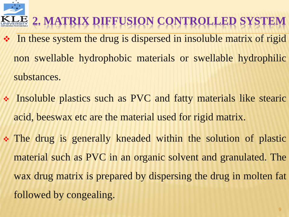
In these system the drug is dispersed in insoluble matrix of rigid

non swellable hydrophobic materials or swellable hydrophilic

substances.

Insoluble plastics such as PVC and fatty materials like stearic

acid, beeswax etc are the material used for rigid matrix.

The drug is generally kneaded within the solution of plastic

material such as PVC in an organic solvent and granulated. The

wax drug matrix is prepared by dispersing the drug in molten fat

followed by congealing.

9

MATRIX DIFFUSION CONTROLLED SYSTEM

10


• The equation describing drug release for this system is given

by T. Higuchi.

Q=[Dἐ /T (La-ἐCs)Cs t]1/2

Q = weight in gram of drug release/unit surface area

D = diffusion coefficient

Cs = solubility of drug in the release medium

ἐ = Porosity of matrix

T = tourtuosity of matrix

A = Concentration of drug in the tablet express as g/ml11


Assumptions made in the previous equations :

A pseudo-steady state is maintained during release .

A>>Cs , i.e. , excess solute is present .

C=0 in solution at all times ( perfect sink ) .

Drug particles are much smaller than those in the matrix .

The diffusion coefficient remains constant .

No interaction between the drug and the matrix occurs .

12


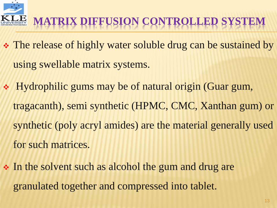
The release of highly water soluble drug can be sustained by

using swellable matrix systems.

Hydrophilic gums may be of natural origin (Guar gum,

tragacanth), semi synthetic (HPMC, CMC, Xanthan gum) or

synthetic (poly acryl amides) are the material generally used

for such matrices.

In the solvent such as alcohol the gum and drug are

granulated together and compressed into tablet.

13


The mechanism of drug release from this system involves

initial dehydration of hydrogel followed by absorption of

water and desorption of drug via swelling controlled

diffusion mechanism.

As the gum swells and the drug diffuses out of it, the

swollen mass devoid of drug appear transparent or glass like

and so the system is sometimes called as glassy hydrogel.

14

Advantages and Disadvantages of Matrix and

Reservoir system

Matrix system Reservoir system

Suitable for both non- Degradable reservoir systems

degradable and degradable system. may be difficult to design

No danger of ‘dose dumping’ Rupture can result in dangerous

in case of rupture. Dose dumping.

Achievement of ‘zero order’ Achievement of zero order

release is difficult. release is easy.

15

DISSOLUTION CONTROLLED RELEASE

These system are easiest to design.

The drug with slow dissolution rate is inherently sustained.

E.g. Griseofulvin, Digoxin and Saliyclamide & they act as

natural prolonged release products.

16

Aluminum aspirin and ferrous sulfate produce slow

dissolving form when it comes in contact with GI fluids.

Drugs having high aqueous solubility & dissolution rate

E.g. Pentoxifylline steroid undergo transformation into less

soluble polymorphs during dissolution in absorption pool.


17


The basic principle of dissolution control is as follows: If the

dissolution process is diffusion layer controlled where the rate

of diffusion from the solid surface through a unstirred liquid

film to the bulk solution is rate limiting, the flux ‘J’ is given by

J= -D(dc/dx)

Where,

D = Diffusion coefficient.

Dc/ dx = Concentration gradient between the solid surface and

bulk of solution.18

In terms of flow rate of material (dm/dt) through unit area (A), the

flux can be given as

J = (1/A) dm/dt

For the system with linear concentration gradient and thickness of the

diffusion layer ‘h’

dc/ dx = (Cb - Cs)

Where Cs represents the concentration at the solid surface and Cb is

the bulk solution concentration. A combined equation for rate of

material is given as

dm/dt = - (DA/h) (Cb - Cs) = kA (Cs - Cb)

Where, k is intrinsic dissolution rate constant.


19

Dissolution controlled release products are divided

in two classes:

1) Encapsulation dissolution control.

2) Matrix dissolution control.

1. Encapsulation/Coating dissolution controlled system

(Reservoir Devices):

Encapsulation involves coating of individual particles, or

granules of drug with the slowly dissolving material.

The particles obtained after coating can be compressed

directly into tablets as in spacetabs or placed in capsules as

in the spansule products.20

Encapsulation/Coating dissolution controlled

system (Reservoir Devices):

As the time required for dissolution of coat is a function of

its thickness and the aqueous solubility of the polymer one

can obtain the coated particles of varying thickness in the

range of 1- 200 micron.

21



By using one of several microencapsulation techniques the

drug particles are coated or encapsulated with slowly

dissolving materials like cellulose, PEGs, olymethacrylates,

waxes etc.

Two methods of preparation are employed :

1. Seed or granule coating

2. Microencapsulation

22

Seed or Granule Coated Products :

Procedure:

Non pareil seeds are coated with drug

This followed with by a coat of slowly dissolving material such as

carbohydrate sugars & cellulose , PEG , polymeric material & wax.

Coated granules can be placed in a capsule for administration.

E.g. amobarbital & dextroamphetamine sulfate

Microencapsulation :

• This method can be used to encase liquids , solids , or gases.

E.g. aspirin & potassium chloride

• Advantage of this method is that sustained drug release can be

achieved with taste abatement & better GI tolerability.



23

MICROENCAPSULATION PROCESSES

PROCESSES TYPES OF MATERIALS FOR

COATING

COASERVATION/ PHASE

SEPARATION

WATER –SOLUBLE POLYMER

INTERFACIAL

POLYMERIZATION

WATER-INSOLUBLE &WATER

SOLUBLE MONOMER

ELECTOSTATIC METHOD OPPOSITELY CHARGED

AEROSOLS

PRECIPITATION WATER OR SOLVENT-SOLUBLE

POLYMER

HOT MELT LOW MOLECULAR WEIGHT

LIPIDS

SALTING OUT WATER-SOLUBLE POLYMERS

SOLVENT EVAPORATION SOLVENT-SOLUBLE POLYMERS

24

2. Matrix (or Monolith)/ Embedded dissolution controlled system.

Since the drug is homogeneously dispersed throughout a rate

controlling medium matrix system are also called monoliths.

The waxes used for such system are beeswax, carnauba wax,

hydrogenated castor oil etc.

These waxes control the drug dissolution by controlling the rate

of dissolution fluid penetration into the matrix by altering the

porosity of tablet, decreasing its wettability or by itself dissolved

at a slower rate. 25

Matrix (or Monolith)/ Embedded dissolution

controlled system.

The dispersion of drug wax is prepared by dispersing the drug in

the molten wax followed by congealing and granulating the

same.

The process, compression parameters and size of particles

formed determine the release rate from this system. The drug

release is often first order from such matrices.

26

Matrix (or Monolith)/ Embedded dissolution

controlled system.

27

MARKETED FORMULATIONS

Dosage form Nature of chemical

entity

Release

mechanism

Company

Geomatrix Multilayered

tablets

- Dissolution Skye

pharmaceuticals,p

lc., (USA).

Reduced irritation

system

Capsules - Dissolution DepoMed, Inc.

Dimatrix

(Diffusion

consulted matrix

system)

Tablets - Dosage form Biovail

corporation

international,

IDDAS (Intestinal

Protective Drug

Absorption)

system

Tablets Hydrophillic

compounds

Diffusion Elan corporation

Multipor Tablets - Diffusion Ethical

Holding,plc.,

(UK).

PPDS (Pellatized

Pulsatile Delivery

Pellets (tablets) - Diffusion Andrx

pharmaceuticals. 28

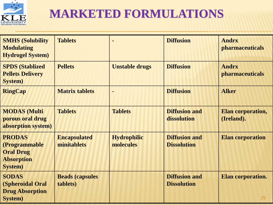
SMHS (Solubility

Modulating

Hydrogel System)

Tablets - Diffusion Andrx

pharmaceuticals

SPDS (Stablized

Pellets Delivery

System)

Pellets Unstable drugs Diffusion Andrx

pharmaceuticals

RingCap Matrix tablets - Diffusion Alker

MODAS (Multi

porous oral drug

absorption system)

Tablets Tablets Diffusion and

dissolution

Elan corporation,

(Ireland).

PRODAS

(Programmable

Oral Drug

Absorption

System)

Encapsulated

minitablets

Hydrophilic

molecules

Diffusion and

Dissolution

Elan corporation

SODAS

(Spheroidal Oral

Drug Absorption

System)

Beads (capsules

tablets)

Diffusion and

Dissolution

Elan corporation.

MARKETED FORMULATIONS

29

EROSION CONTROLLED DRUG DELIVERY

SYSTEM

Erosion is defined as the disintegration of the polymer/ wax

matrix, as a result of degradation and is characterized by

material loss from the polymer generally in the physical state.

Polymer or wax degradation or hydrolysis is brought by

enzyme, pH change or due to osmotic pressure or hydrodynamic

pressure that causes fragmentation.

Erosion is effected by external stimuli, such systems can be

classified under stimuli activated drug delivery system.30


SYSTEM

It is classified on the type of stimuli:

1. Physical e.g. (osmotic pressure)

2. Chemical e.g.(pH)

3. Biological e.g. (enzyme)

Examples of erodible matrices include hydrophobic

materials ethyl cellulose and waxes.

Depending on the erosion mechanism, polymer or waxes

undergo either surface erosion or bulk erosion31


SYSTEM

a) SURFACE EROSION:

It occurs from the surface layers of the device only.

It results in gradual decrease in the size of the device while

the bulk phase remain un-degraded.

There is a difference in erosion rate between the surface

and centre of matrix, the process is also called as

heterogeneous erosion.

Surface erosion occurs when water penetration is

restricted to device surface.32


SYSTEMb) BULK EROSION:

it occurs throughout the polymer bulk and the process is

thus called as homogenous erosion.

Bulk erosion occurs when the water is readily able to

penetrate the matrix of the device.

34

HYBRID SYSTEM IN DRUG DELIVERY

They are also called as membrane cum matrix drug delivery

system.

These systems are those where the drug in matrix of release-

retarding material is further coated with a release

controlling polymer membrane.

It combines constant release kinetics of reservoir system

with mechanical robustness of matrix system. 35


SYSTEM

Degradation by erosion normally takes place in devices that are

prepared from soluble polymers.

In such instances, the device erodes as water is absorbed into the

systems causing the polymer chains to hydrate, swell, and ultimately

dissolved away from the dosage form.

Degradation can also result from chemical changes to the polymer

including cleavage of covalent bonds, ionization and protonation

either along the polymer backbone or on pendent side chains.36

MATHEMATICAL MODELS

There are various mathematical models

1) Zero order kinetics

2) First order kinetics

3) Weibull model

4) Higuchi model

5) Hixson Crowell model

6) Korsmeyer Peppas model

7) Baker- Lonsdale model

8) Hopfenberg model37

ZERO ORDER KINETICS

This model is used for dosage forms that do not

disaggregate and release the drug slowly (assuming that

area does not change and no equilibrium conditions are

obtained).

It can be represented by the following equation:

Wo - Wt = Kt

39

Wo - Wt = Kt

Where W is the initial amount of drug in the pharmaceutical

dosage form, W is the amount of drug in the pharmaceutical

dosage form at time t and K is a proportionality constant.

Dividing this equation by W0 and simplifying.

ft= kot

Where ft = 1-(Wt –W0) and f represents the fraction of drug

dissolved in time t and k0 the apparent dissolution rate

constant or zero order release constant.40

FIRST ORDER KINETICS

This model is applied for dissolution studies, and also

describe the absorption and elimination of some drugs.

ln Qt = ln Q0 + Kt

Qt = Drug amounts remaining to be released at time t

Q0 = Drug amounts remaining to be released at zero hr

Kt = First order release constant.

A graph of drug release versus time will be linear.

41

WEIBULL MODEL

A general empirical equation adopted by Weibull was used

to describe the release process.

Erodible matrix formulations follow this model.

M = 1- e[-(t-Ti)b/a

42

HIGUCHI MODEL

Diffusion matrix formulations follow this model.

This model is used to study the release of water soluble and

low soluble drugs incorporated in semisolid and / or solid

matrixes.

It is denoted by the following equation

ft = KHt1/2

ft = fraction of drug released at time t

KH = Higuchi release rate constant

t = time43

HIXSON – CROWELL MODEL

Erodible matrix systems follow this model.

When this model is used, it is assumed that release rate is

limited by the drug particles dissolution rate, and not by the

diffusion that may occur through polymeric matrix.

It is represented by the following equation

Wo1/3 – Wt1/3= Kst

44

HIXSON – CROWELL MODEL

Wo1/3 – Wt1/3= Kst

Where,

Wo = initial amount of drug present in the matrix.

Wt = amount of drug released in time t.

Ks = release rate constant.

45

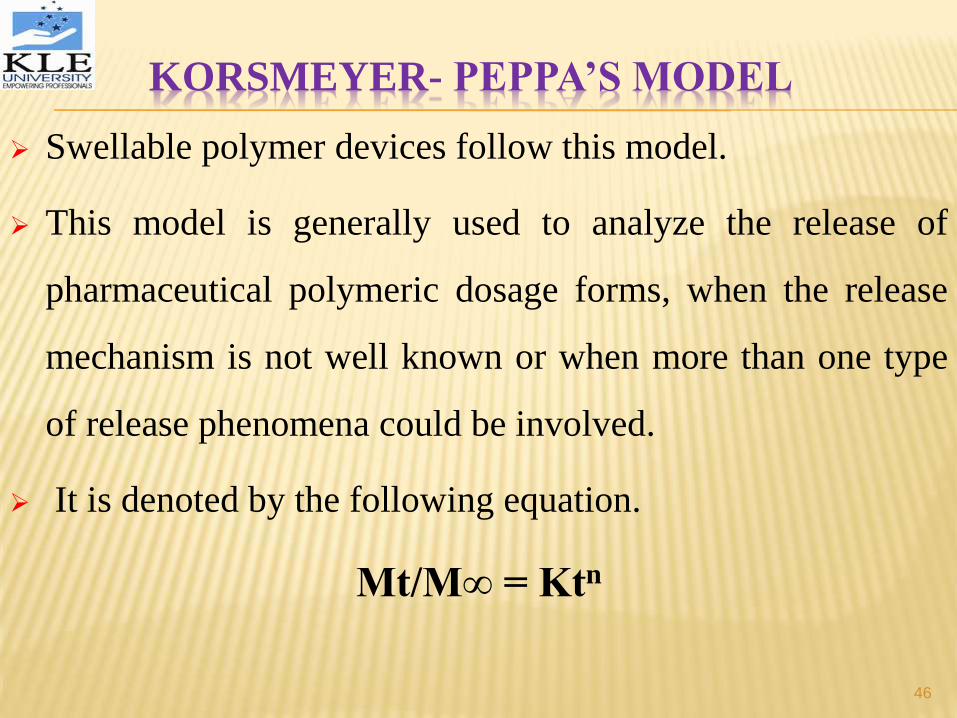
KORSMEYER- PEPPA’S MODEL

Swellable polymer devices follow this model.

This model is generally used to analyze the release of

pharmaceutical polymeric dosage forms, when the release

mechanism is not well known or when more than one type

of release phenomena could be involved.

It is denoted by the following equation.

Mt/M∞ = Ktn

46

KORSMEYER- PEPPA’S MODEL

Mt/M∞ = Ktn

Where,

Mt = amount released at time t

M∞= amount released at infinite time

K = release rate constant

n = release exponents

47

BAKER- LANSDALE MODEL

This model is suitable for microcapsules or microspheres.

It describes the drug controlled release from a spherical

matrix.

ft = 3/2[1-(1-Mt/M∞)2/3] – Mt/M∞= Kt

Where,

Ft = fraction of drug released at time t


M∞ = amount released at infinite time48

HOPFENBERG MODEL

This model was used for the release of drugs from surface-

eroding devices with several geometries.

This equation describes drug release from slabs, spheres and

infinite cylinders displaying heterogeneous erosion.

It is given by the following the equation.

Mt/M∞ 1 – [1-k1t(t-l)]n

49

HOPFENBERG MODEL


M∞ = amount released at infinite time

K = rate constant

Mt/M∞ 1 – [1-k1t(t-l)]n

50

OPTIMIZATION TECHNIQUES IN

PHARMACEUTICAL FORMULATION

AND PROCESSING

51

CONTENTS

CONCEPT OF OPTIMIZATION

OPTIMIZATION PARAMETERS

CLASSICAL OPTIMIZATION

STATISTICAL DESIGN

DESIGN OF EXPERIMENT

OPTIMIZATION METHODS

52

INTRODUCTION

The term Optimize is defined as “to make perfect”.

It is used in pharmacy relative to formulation and processing

Involved in formulating drug products in various forms

It is the process of finding the best way of using the existing

resources while taking in to the account of all the factors that

influences decisions in any experiment53

In development projects , one generally experiments by a

series of logical steps, carefully controlling the variables &

changing one at a time, until a satisfactory system is

obtained

It is not a screening technique.

Optimization tech provide both depth of understanding &

ability to explore & defend range for formulation &

processing factors.

INTRODUCTION

54

OPTIMIZATION PARAMETERS

optimization parameters

Problem types variable

Constrained unconstrained dependent independent

55

VARIABLES

Independent Dependent

Formulating processing

Variables Variables

56

Independent variables or primary variables :

Formulations and process variables are directly

under control of the formulator. These includes

ingredients

Dependent or secondary variables :

These are the responses of the in progress material

or the resulting drug delivery system. It is the result of

independent variables

VARIABLES

57

Relationship between independent variables and response

defines response surface.

Representing >2 becomes graphically impossible

Higher the variables , higher are the complications hence it

is to optimize each & everyone.

VARIABLES

58

Response surface representing the relationship between the

independent variables X1 and X2 and the dependent variable

Y.

VARIABLES

59

CLASSIC OPTIMIZATION

It involves application of calculus to basic problem for

maximum/minimum function.

Applications:

i. Problems that are not too complex

ii. They do not involve more than two variables

For more than two variables graphical representation is

impossible.

It is possible mathematically.

60

GRAPH REPRESENTING THE RELATION

BETWEEN THE RESPONSE VARIABLE AND

INDEPENDENT VARIABLE

61

Using calculus the graph obtained can be solved.

Y = f (x)

When the relation for the response y is given as the function of two

independent variables,X1 &X2

Y = f(X1 , X2)

The above function is represented by contour plots on which the axes

represents the independent variables X1& X2

CLASSIC OPTIMIZATION

62

STATISTICAL DESIGN

These Techniques are divided in to two types.

Experimentation continues as optimization proceeds

It is represented by evolutionary operations(EVOP) and

simplex methods.

Experimentation is completed before optimization takes

place.

It is represented by classic mathematical & search

methods.63

There are two possible approaches

Theoretical approach- If theoretical equation is known , no

experimentation is necessary.

Empirical or experimental approach – With single

independent variable formulator experiments at several

levels.

STATISTICAL DESIGN

64

The relationship with single independent variable can be obtained by

simple regression analysis or by least squares method.

The relationship with more than one important variable can be

obtained by statistical design of experiment and multi linear

regression analysis.

Most widely used experimental plan is factorial design.

STATISTICAL DESIGN

65

TERMS USED

FACTOR: It is an assigned variable such as concentration ,Temperature etc..,

Quantitative: Numerical factor assigned to it

Ex; Concentration- 1%, 2%,3% etc..

Qualitative: Which are not numerical

Ex; Polymer grade, humidity condition etc

LEVELS: Levels of a factor are the values or designationsassigned to the factor

FACTOR LEVELS

Temperature 300 , 500

Concentration 1%, 2%

66

RESPONSE: It is an outcome of the experiment.

It is the effect to evaluate.

Ex: Disintegration time etc..,

EFFECT: It is the change in response caused by varying the levels

It gives the relationship between various factors & levels

INTERACTION: It gives the overall effect of two or more variables

Ex: Combined effect of lubricant and glidant on hardness of the tablet

TERMS USED

67

Optimization by means of an experimental design may be helpful in

shortening the experimenting time.

The design of experiments is a structured , organized method used to

determine the relationship between the factors affecting a process and

the output of that process.

Statistical DOE refers to the process of planning the experiment in

such a way that appropriate data can be collected and analyzed

statistically.

TERMS USED

68

TYPES OF EXPERIMENTAL DESIGN

Completely randomized designs

Randomized block designs

Factorial designs

Full

Fractional

Response surface designs

Central composite designs

Box-Behnken designs

Adding centre points

Three level full factorial designs

69

Completely randomised Designs

These experiments compares the values of a response variable based

on different levels of that primary factor.

For example ,if there are 3 levels of the primary factor with each level

to be run 2 times then there are 6 factorial possible run sequences.

Randomised block designs

For this there is one factor or variable that is of primary interest.

To control non-significant factor, an important technique called

blocking can be used to reduce or eliminate the contribution of these

factors to experimental error.

TYPES OF EXPERIMENTAL DESIGN

70

Full: used for small set of factors

Fractional: used to examine multiple factors efficiently with fewer

runs than corresponding full factorial design

Types of fractional factorial designs

Homogenous fractional

Mixed level fractional

Box-Hunter

Plackett-Burman

Taguchi

Latin square

FACTORIAL DESIGN

71

Homogenous fractional

Useful when large number of factors must be screened.

Mixed level fractional

Useful when variety of factors need to be evaluated for main

effects and higher level interactions can be assumed to be

negligible.

Box-hunter

Fractional designs with factors of more than two levels can be

specified as homogenous fractional or mixed level fractional.

FACTORIAL DESIGN

72

PLACKETT-BURMAN

It is a popular class of screening design.

These designs are very efficient screening designs when only the

main effects are of interest.

These are useful for detecting large main effects economically

,assuming all interactions are negligible when compared with

important main effects.

Used to investigate n-1 variables in n experiments proposing

experimental designs for more than seven factors and especially

for n*4 experiments.

73

TAGUCHI:

It allows estimation of main effects while minimizing variance.

LATIN SQUARE:

They are special case of fractional factorial design where there is

one treatment factor of interest and two or more blocking

factors.

FACTORIAL DESIGN

74

RESPONSE SURFACE DESIGNS

This model has quadratic form

Designs for fitting these types of models are known as response

surface designs.

If defects and yield are the outputs and the goal is to minimize

defects and maximize yield

γ =β0 + β1X1 + β2X2 +….β11X12 + β22X2

2

75

Two most common designs generally used in this response surface

modeling are :

Central composite designs

Box-Behnken designs

Box-Wilson central composite Design

This type contains an embedded factorial or fractional factorial design

with centre points that is augmented with the group of ‘star points’.

These always contains twice as many star points as there are factors in

the design.


76

The star points represent new extreme value (low & high) for each factor in

the design.

To picture central composite design, it must imagined that there are several

factors that can vary between low and high values.

Central composite designs are of three types

Circumscribed designs-Cube points at the corners of the unit cube ,star

points along the axes at or outside the cube and centre point at origin

Inscribed designs-Star points take the value of +1 & -1 and cube points lie

in the interior of the cube

Faced –star points on the faces of the cube.


77

BOX-BEHNKEN DESIGN

They do not contain embedded factorial or fractional

factorial design.

Box-Behnken designs use just three levels of each factor.

These designs for three factors with circled point appearing

at the origin and possibly repeated for several runs.

78

Three-level full factorial designs

It is written as 3k factorial design.

It means that k factors are considered each at 3 levels.

These are usually referred to as low, intermediate & high

values.

These values are usually expressed as 0, 1 & 2

The third level for a continuous factor facilitates

investigation of a quadratic relationship between the

response and each of the factors.

79

FACTORIAL DESIGN

These are the designs of choice for simultaneous determination

of the effects of several factors & their interactions.

They are used in experiments where the effects of different

factors or conditions on experimental results are to be elucidated.

Two types

Full factorial- Used for small set of factors

Fractional factorial- for optimizing more number of factors

80

LEVELS OF FACTORS IN THIS FACTORIAL DESIGN

FACTOR

LOWLEVEL(mg)

HIGH LEVEL(mg)

A:stearate 0.5 1.5

B:Drug 60.0 120.0

C:starch 30.0 50.0

81

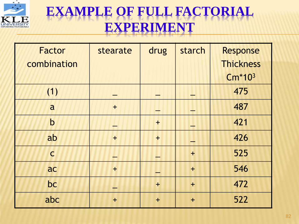
EXAMPLE OF FULL FACTORIAL

EXPERIMENT

Factor

combination

stearate drug starch Response

Thickness

Cm*103

(1) _ _ _ 475

a + _ _ 487

b _ + _ 421

ab + + _ 426

c _ _ + 525

ac + _ + 546

bc _ + + 472

abc + + + 522

82

Calculation of main effect of A (stearate)

The main effect for factor A is

{-(1)+a-b+ab-c+ac-bc+abc] 10-3

Main effect of A =

=

= 0.022 cm

4

a + ab + ac + abc

4

_ (1) + b + c + bc

4

[487 + 426 + 456 + 522 – (475 + 421 + 525 + 472)] 10-3

EXAMPLE OF FULL FACTORIAL

EXPERIMENT

83

GENERAL OPTIMIZATION

By the relationships are generated from experimental data ,

resulting equations are on the basis of optimization.

These equation defines response surface for the system

under investigation.

After collection of all the runs and calculated responses

,calculation of regression coefficient is initiated.

Analysis of variance (ANOVA) presents the sum of the

squares used to estimate the factor main effects.

84

FLOW CHART FOR OPTIMIZATION

85

APPLIED OPTIMIZATION METHODS

Evolutionary operations

Simplex method

Lagrangian method

Search method

Canonical analysis

86

EVOLUTIONARY OPERATIONS (EVOP)

It is a method of experimental optimization.

Technique is well suited to production situations.

Small changes in the formulation or process are

made (i.e. repeats the experiment so many times)

& statistically analyzed whether it is improved.

It continues until no further changes takes place

i.e., it has reached optimum-the peak

87

Applied mostly to TABLETS.

Production procedure is optimized by careful

planning and constant repetition

It is impractical and expensive to use.

It is not a substitute for good laboratory scale

investigation

EVOLUTIONARY OPERATIONS (EVOP)

88

SIMPLEX METHOD

It is an experimental method applied for

pharmaceutical systems.

Technique has wider appeal in analytical method other

than formulation and processing.

Simplex is a geometric figure that has one more point

than the no. of factors.

It is represented by triangle.

It is determined by comparing the magnitude of the

responses after each successive calculation

89

GRAPH REPRESENTING THE SIMPLEX MOVEMENTS TO THE

OPTIMUM CONDITIONS

90

The two independent variables show pump speeds for the two

reagents required in the analysis reaction.

Initial simplex is represented by lowest triangle.

The vertices represents spectrophotometric response.

The strategy is to move towards a better response by moving

away from worst response.

Applied to optimize CAPSULES, DIRECT COMPRESSION

TABLET (acetaminophen), liquid systems (physical stability)

SIMPLEX METHOD

91

LAGRANGIAN METHOD

It represents mathematical techniques.

It is an extension of classic method.

It is applied to a pharmaceutical formulation and processing.

This technique follows the second type of statistical design.

Limited to 2 variables - disadvantage

92

STEPS INVOLVED

Determine objective formulation

Determine constraints.

Change inequality constraints to equality constraints.

Form the Lagrange function F

Partially differentiate the lagrange function for each variable

& set derivatives equal to zero.

Solve the set of simultaneous equations.

Substitute the resulting values in objective functions93

Optimization of a tablet.

phenyl propranolol (active ingredient)- kept constant

X1 – disintegrate (corn starch)

X2 – lubricant (stearic acid)

X1 & X2 are independent variables.

Dependent variables include tablet hardness, friability

,volume, in-vitro release rate etc.,

STEPS INVOLVED (EXAMPLE)

94

Polynomial models relating the response variables to independents

were generated by a backward stepwise regression analysis program.

Y= B0+B1X1+B2X2+B3 X12 +B4 X2

2 +B+5 X1 X2 +B6 X1X2

+ B7X12+B8X1

2X22

Y – response

Bi – regression coefficient for various terms containing the levels of

the independent variables.

X – independent variables

STEPS INVOLVED (EXAMPLE)

95

TABLET FORMULATIONS

Formulation

no,.

Drug Dicalcium

phosphate

Starch Stearic acid

1 50 326 4(1%) 20(5%)

2 50 246 84(21%) 20

3 50 166 164(41%) 20

4 50 246 4 100(25%)

5 50 166 84 100

6 50 86 164 100

7 50 166 4 180(45%)

96

Constrained optimization problem is to locate the levels of stearic

acid (x1) and starch (x2).

This minimize the time of in-vitro release(y2),average tablet

volume(y4), average friability (y3)

To apply the lagrangian method, problem must be expressed

mathematically as follows

Y2 = f2(X1,X2) - in vitro release

Y3 = f3(X1,X2) < 2.72-Friability

Y4 = f4(x1,x2) < 0.422-avg tab.vol

LAGRANGIAN METHOD

97

CONTOUR PLOT FOR TABLET HARDNESS

98

CONTOUR PLOT FOR TABLET

DISSOLUTION(T50%)

99

GRAPH OBTAINED BY SUPER IMPOSITION OF

TABLET HARDNESS & DISSOLUTION

100

CONTOUR PLOT FOR TABLET FRIABILITY

101

SEARCH METHOD

It is defined by appropriate equations.

It do not require continuity or differentiability of function.

It is applied to pharmaceutical system

For optimization 2 major steps are used

Feasibility search - used to locate set of response constraints

that are just at the limit of possibility.

Grid search – experimental range is divided in to grid of

specific size & methodically searched102

STEPS INVOLVED IN SEARCH METHOD

Select a system

Select variables

Perform experiments and test product

Submit data for statistical and regression analysis

Set specifications for feasibility program

Select constraints for grid search

Evaluate grid search printout

103

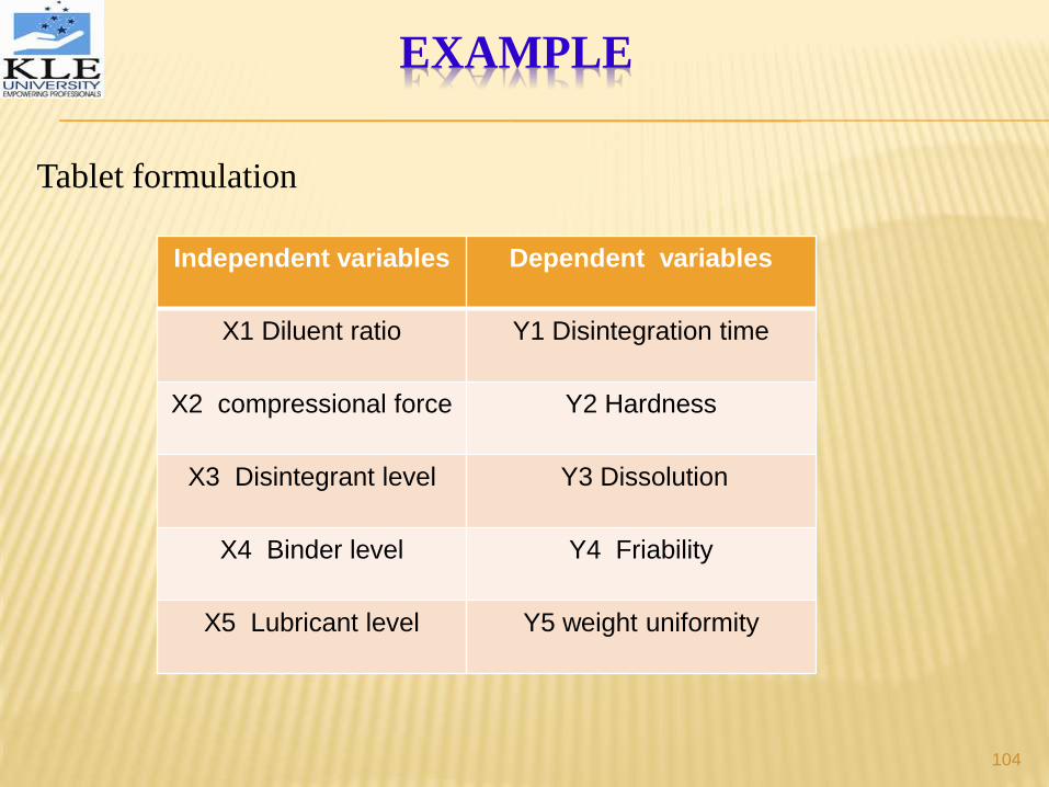
EXAMPLE

Tablet formulation

Independent variables Dependent variables

X1 Diluent ratio Y1 Disintegration time

X2 compressional force Y2 Hardness

X3 Disintegrant level Y3 Dissolution

X4 Binder level Y4 Friability

X5 Lubricant level Y5 weight uniformity

104

Five independent variables dictates total of 32

experiments.

This design is known as five-factor,orthagonal,central

,composite , second order design.

First 16 formulations represent a half-factorial design for

five factors at two levels .

The two levels represented by +1 & -1, analogous to high

& low values in any two level factorial.

SEARCH METHOD

105

TRANSLATION OF STATISTICAL DESIGN IN TO PHYSICAL UNITS

Experimental conditions

Factor -1.54eu -1 eu Base0 +1 eu +1.54eu

X1=

ca.phos/lactose

24.5/55.5 30/50 40/40 50/30 55.5/24.5

X2= compression

pressure( 0.5 ton)

0.25 0.5 1 1.5 1.75

X3 = corn starch

disintegrant

2.5 3 4 5 5.5

X4 = Granulating

gelatin(0.5mg)

0.2 0.5 1 1.5 1.8

X5 = mg.stearate

(0.5mg)

0.2 0.5 1 1.5 1.8

106

Again formulations were prepared and are measured.

Then the data is subjected to statistical analysis followed by

multiple regression analysis.

The equation used in this design is second order

polynomial.

y = a0+a1x1+…+a5x5+a11x12+…+a55x

25+a12x1x2

+a13x1x3+a45 x4x5

SEARCH METHOD

107

A multivariant statistical technique called principle

component analysis (PCA) is used to select the best

formulation.

PCA utilizes variance-covariance matrix for the

responses involved to determine their interrelationship.

SEARCH METHOD

108

PLOT FOR A SINGLE VARIABLE

109

PLOT OF FIVE VARIABLES

110

PLOT OF FIVE VARIABLES

111

ADVANTAGES OF SEARCH METHOD

It takes five independent variables in to account.

Persons unfamiliar with mathematics of optimization &

with no previous computer experience could carryout an

optimization study.

112

CANONICAL ANALYSIS

It is a technique used to reduce a second order

regression equation.

This allows immediate interpretation of the

regression equation by including the linear and

interaction terms in constant term.

113

It is used to reduce second order regression equation to an

equation consisting of a constant and squared terms as

follows.

It was described as an efficient method to explore an

empherical response.Y = Y0 +λ1W1

2 + λ2W22 +..

CANONICAL ANALYSIS

114

Thank you

E-mail: [email protected]

Cell No:00919742431000

115

fundamentals of modified release formulations

Education

release of drug

diffusion of dissolved

core of drug

rate of drug release

cases drug

additional drug

diffusion coefficient

diffusion controlledthere