fundamentals of control systemshthoang/cstd/fundctrlsys_chapter6.pdf · fundamentals of control...
TRANSCRIPT

Lecture NotesLecture Notes
Fundamentals of Control SystemsFundamentals of Control Systems
Instructor: Assoc. Prof. Dr. Huynh Thai HoangDepartment of Automatic Control
Faculty of Electrical & Electronics EngineeringHo Chi Minh City University of Technology
Email: [email protected]@yahoo.com
Homepage: www4.hcmut.edu.vn/~hthoang/
6 December 2013 © H. T. Hoang - www4.hcmut.edu.vn/~hthoang/ 1

Chapter 6Chapter 6
DESIGN OF CONTINUOUS DESIGN OF CONTINUOUS CONTROL SYSTEMSCONTROL SYSTEMS
6 December 2013 © H. T. Hoàng - www4.hcmut.edu.vn/~hthoang/ 2

Introduction
ContentContent
Introduction Effect of controllers on system performance Control systems design using the root locus method Control systems design using the root locus method Control systems design in the frequency domain Design of PID controllersg Control systems design in state-space Design of state estimators
6 December 2013 © H. T. Hoàng - www4.hcmut.edu.vn/~hthoang/ 3
IntroductionIntroduction
6 December 2013 © H. T. Hoàng - www4.hcmut.edu.vn/~hthoang/ 4
Introduction to design processIntroduction to design process
Design is a process of adding/configuring hardware as well assoftware in a system so that the new system satisfies thed i d ifi tidesired specifications.
6 December 2013 © H. T. Hoàng - www4.hcmut.edu.vn/~hthoang/ 5

The controller is connected in series with the plant
Series compensatorSeries compensator
The controller is connected in series with the plant.
R(s)G(s)+
Y(s)GC(s)
Controllers: phase lead, phase lag, lead-lag compensator, P,PD PI PIDPD, PI, PID,…
Design method: root locus frequency response
6 December 2013 © H. T. Hoàng - www4.hcmut.edu.vn/~hthoang/ 6
Design method: root locus, frequency response

State feedback controlState feedback control
All the states of the system are fed back to calculate the control All the states of the system are fed back to calculate the controlrule.
+r(t) u(t)
C y(t))()()( tutt BAxx
x(t)
K
State feedback controller: )()()( ttrtu Kx
Design method: pole placement LQR
nkkk 21K
6 December 2013 © H. T. Hoàng - www4.hcmut.edu.vn/~hthoang/ 7
Design method: pole placement, LQR,…

Effects of controller on systemEffects of controller on systemEffects of controller on system Effects of controller on system performanceperformance
6 December 2013 © H. T. Hoàng - www4.hcmut.edu.vn/~hthoang/ 8

The addition of a pole (in the left-half s-plane) to the open-
Effects of the addition of polesEffects of the addition of poles The addition of a pole (in the left half s plane) to the open
loop transfer function has the effect of pushing the root locusto the right, tending to lower the system’s relative stability andt l d th ttli f thto slow down the settling of the response.
Im s Im s Im s
Re s Re s Re s
6 December 2013 © H. T. Hoàng - www4.hcmut.edu.vn/~hthoang/ 9
The addition of a zero (in the left-half s-plane) to the open-
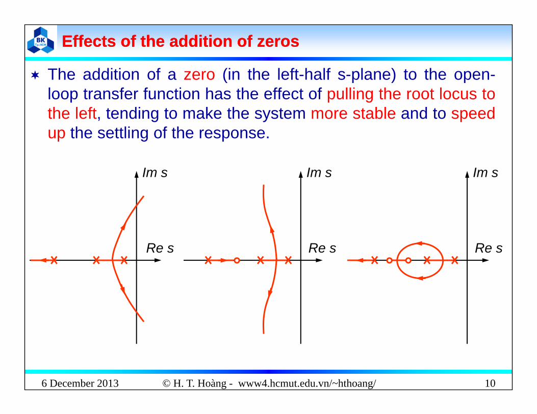
Effects of the addition of zerosEffects of the addition of zeros
The addition of a zero (in the left half s plane) to the openloop transfer function has the effect of pulling the root locus tothe left, tending to make the system more stable and to speed
th ttli f thup the settling of the response.
Im s Im s Im s
Re s Re s Re s
6 December 2013 © H. T. Hoàng - www4.hcmut.edu.vn/~hthoang/ 10
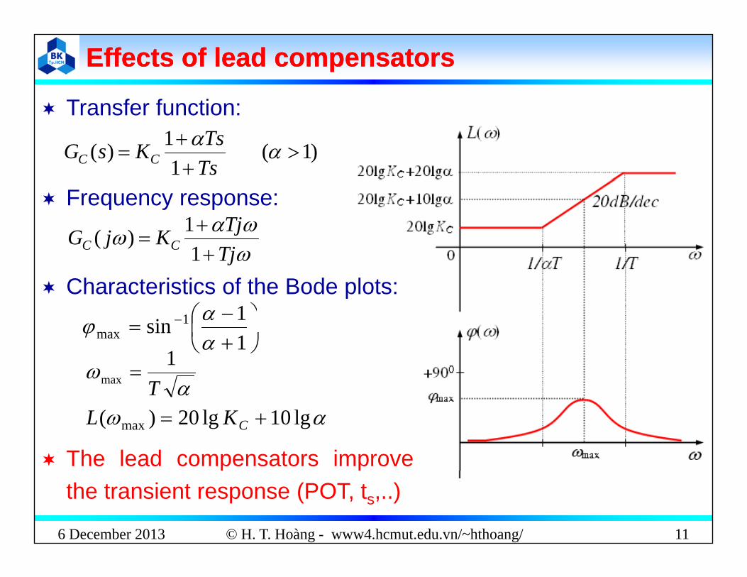
Effects of lead compensatorsEffects of lead compensators
Transfer function:
)1( 1
1)(
TsTsKsG CC
Transfer function:
Frequency response:
TjTjKjG CC
11)(
Tj1
1sin 1
Characteristics of the Bode plots:
1
sinmax
T1
max
lg10lg20)( max CKL
The lead compensators improve
6 December 2013 © H. T. Hoàng - www4.hcmut.edu.vn/~hthoang/ 11
the transient response (POT, ts,..)
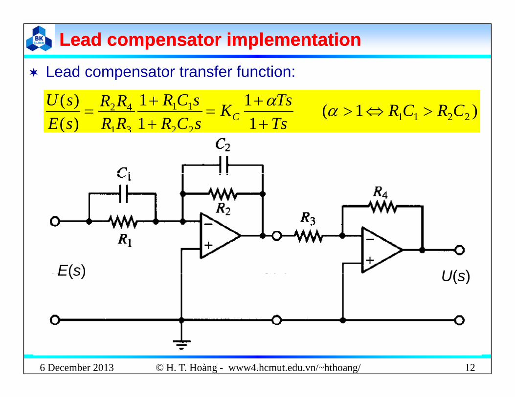
Lead compensator implementationLead compensator implementation Lead compensator transfer function:
)1( 1
1 11
)()(
22111142 CRCR
TsTsK
sCRsCR
RRRR
sEsU
C
Lead compensator transfer function:
11)( 2231 TssCRRRsE
E(s) U(s)E(s) U(s)
6 December 2013 © H. T. Hoàng - www4.hcmut.edu.vn/~hthoang/ 12
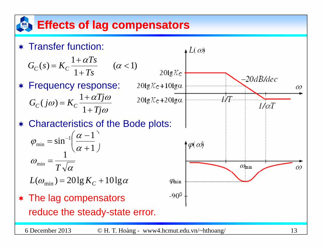
Effects of lag compensatorsEffects of lag compensators
Transfer function:
)1( 1
1)(
TsTsKsG CC
Transfer function:
Frequency response:
TjTjKjG CC
11)(
Tj1
1sin 1
Characteristics of the Bode plots:
1
sinmin
T1
min
lg10lg20)( min CKL
The lag compensators
6 December 2013 © H. T. Hoàng - www4.hcmut.edu.vn/~hthoang/ 13
greduce the steady-state error.

Lag compensator implementationLag compensator implementation Lag compensator transfer function:
)1( 1
1 11
)()(
221122
11
31
42 CRCRTsTsK
sCRsCR
RRRR
sEsU
C
Lag compensator transfer function:
11)( 2231 TssCRRRsE
E(s) U(s)E(s) U(s)
6 December 2013 © H. T. Hoàng - www4.hcmut.edu.vn/~hthoang/ 14

Effects of leadEffects of lead--lag compensatorslag compensators11
sTsT )1,1(
11
11)( 21
2
22
1
11
sTsT
sTsTKsG CC Transfer function:
Bode diagram
The lead lag compensators improve transient response and
6 December 2013 © H. T. Hoàng - www4.hcmut.edu.vn/~hthoang/ 15
The lead-lag compensators improve transient response andreduces the steady-state error.

Effects of proportional controller (P)Effects of proportional controller (P)
G )(T f f ti
Increasing proportional gain leads to decreasing steady-stateh h b l bl d h POT
PC KsG )( Transfer function:
error, however, the system become less stable, and the POTincreases.
(t) Ex: response of a
proportional control t h
y(t)
system whose plant has the transfer functiontransfer function below:
10)(G
6 December 2013 © H. T. Hoàng - www4.hcmut.edu.vn/~hthoang/ 16
)3)(2()(
sssG
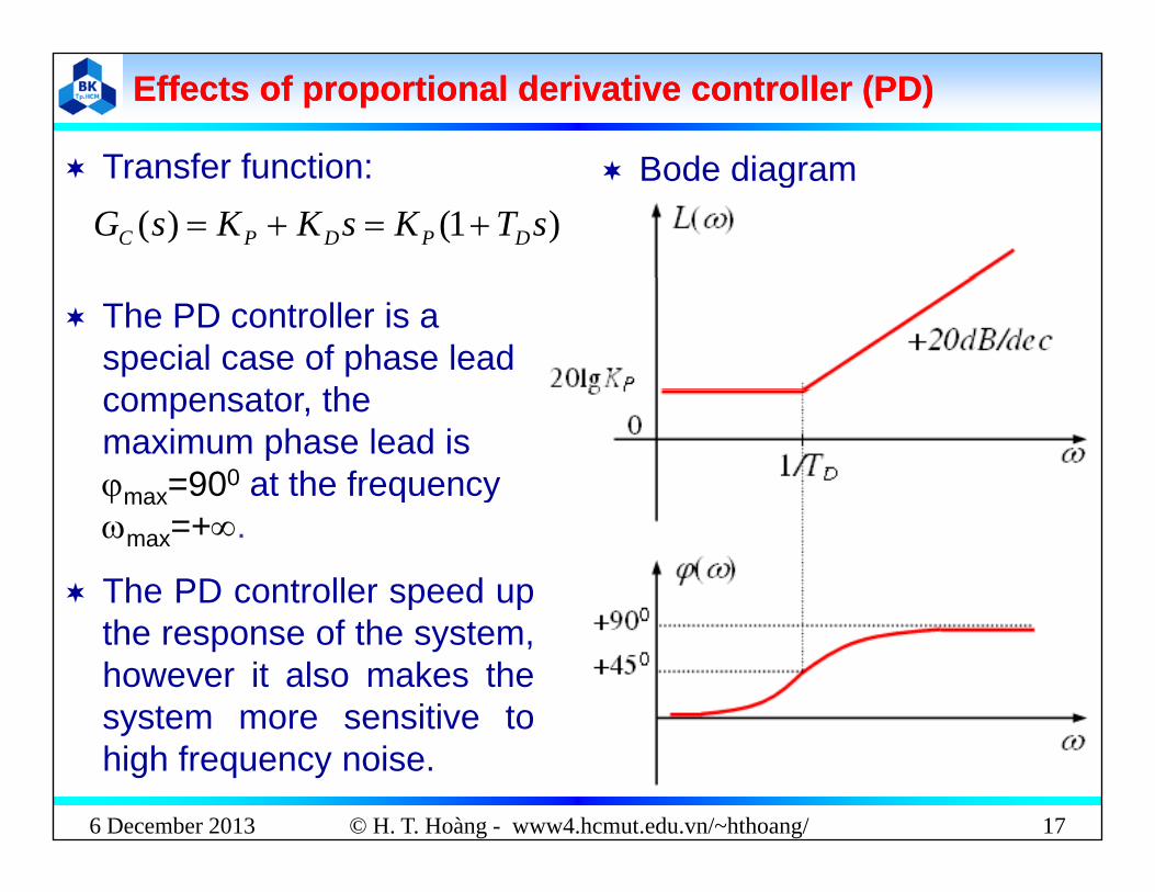
Effects of proportional derivative controller (PD)Effects of proportional derivative controller (PD)
Bode diagram Transfer function: Bode diagram Transfer function:)1()( sTKsKKsG DPDPC
The PD controller is a special case of phase lead
t thcompensator, the maximum phase lead is max=900 at the frequency max q ymax=+.
The PD controller speed upthe response of the system,however it also makes thesystem more sensitive to
6 December 2013 © H. T. Hoàng - www4.hcmut.edu.vn/~hthoang/ 17
system more sensitive tohigh frequency noise.

Effects of proportional derivative controller (PD)Effects of proportional derivative controller (PD)
Note: The larger the derivative constant the faster the Note: The larger the derivative constant, the faster theresponse of the system.
y(t)y( )
unompensated
6 December 2013 © H. T. Hoàng - www4.hcmut.edu.vn/~hthoang/ 18

PD controller implementationPD controller implementation PD controller transfer function:
sKKsCRRRRR
sEsU
DP )1()()(
1142
PD controller transfer function:
RRsE )( 31
E(s)( )U(s)
6 December 2013 © H. T. Hoàng - www4.hcmut.edu.vn/~hthoang/ 19

Effects of proportional integral controller (PI)Effects of proportional integral controller (PI) Transfer function: Bode diagram Transfer function:
)11()(sT
Ks
KKsGI
PI
PC
Bode diagram
The PI controller is a special case of phase lag
t th i icompensator, the minimum phase lag is min= 900 at the frequency min=+.q y min
PI controllers eliminate stead state error to stepsteady state error to step input, however it can increase POT and settling
6 December 2013 © H. T. Hoàng - www4.hcmut.edu.vn/~hthoang/ 20
time.

Effects of proportional integral controller (PI)Effects of proportional integral controller (PI) Note: The larger the integral constant the larger the POT Note: The larger the integral constant, the larger the POT
of response of the system.y(t)y( )
uncompensated
6 December 2013 © H. T. Hoàng - www4.hcmut.edu.vn/~hthoang/ 21

PI controller implementationPI controller implementation PI controller transfer function:
1)()( 2242
sKK
sCRsCR
RRRR
sEsU I
P
PI controller transfer function:
)( 2231 ssCRRRsE
E(s)U( )U(s)
6 December 2013 © H. T. Hoàng - www4.hcmut.edu.vn/~hthoang/ 22
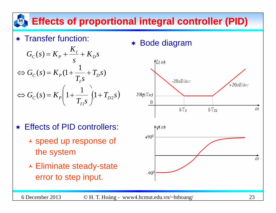
Effects of proportional integral controller (PID)Effects of proportional integral controller (PID) Transfer function:
Bode diagram Transfer function:
sKs
KKsG DI
PC )(
1 )11()( sTsT
KsG DI
PC
TKG 111)(
sT
sTKsG D
IPC 2
1
11)(
Effects of PID controllers:
speed up response of the system
Eliminate steady-state
6 December 2013 © H. T. Hoàng - www4.hcmut.edu.vn/~hthoang/ 23
error to step input.

Comparison of PI, PD and PID controllersComparison of PI, PD and PID controllers
(t)y(t)
U t dUncompensated
6 December 2013 © H. T. Hoàng - www4.hcmut.edu.vn/~hthoang/ 24

Control systems design Control systems design y gy gusing the root locus methodusing the root locus method
6 December 2013 © H. T. Hoàng - www4.hcmut.edu.vn/~hthoang/ 25
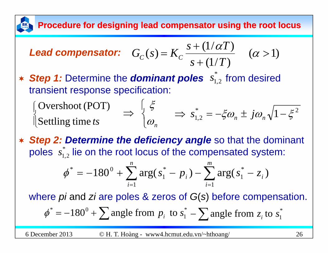
Procedure for designing lead compensator using Procedure for designing lead compensator using the root locusthe root locus
)/1( Ts )1( )/1()/1()(
TsTsKsG CCLead compensator:
Step 1: Determine the dominant poles from desired*s
(POT)Overshoot
2* 1 j
Step 1: Determine the dominant poles from desired transient response specification:
2,1s
Step 2: Determine the deficiency angle so that the dominant
ts timeSettling
( )
n 2
2,1 1 nn js
Step 2: Determine the deficiency angle so that the dominant poles lie on the root locus of the compensated system: *
2,1s
mn
zsps **0* )arg()arg(180
i
ii
i zsps1
11
1 )arg()arg(180
where pi and zi are poles & zeros of G(s) before compensation.
6 December 2013 © H. T. Hoàng - www4.hcmut.edu.vn/~hthoang/ 26
*1
0* to from angle180 spi *1to from angle szi

Procedure for designing lead compensator using the root locusProcedure for designing lead compensator using the root locus
Step 3: Determine the pole & zero of the lead compensator Step 3: Determine the pole & zero of the lead compensatorDraw 2 arbitrarily rays starting from the dominant pole such that the angle between the two rays equal to *. The
*1s
intersection between the two rays and the real axis are the positions of the pole and the zero of the lead compensator. Two methods often used for drawing the rays:Two methods often used for drawing the rays: Bisector method Pole elimination methodPole elimination method
Step 4: Calculate the gain KC using the formula:
1)()( *1
ssC sGsG
6 December 2013 © H. T. Hoàng - www4.hcmut.edu.vn/~hthoang/ 27
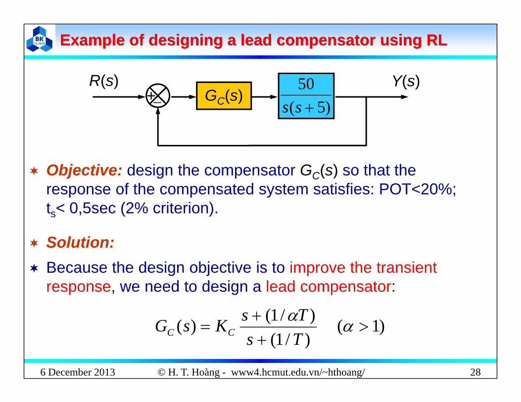
Example of designing a lead compensator using RLExample of designing a lead compensator using RL
( )R(s)+
Y(s)GC(s)
)5(50ss
Objective: design the compensator GC(s) so that the j g p C( )response of the compensated system satisfies: POT<20%; ts< 0,5sec (2% criterion).
Solution: Because the design objective is to improve the transient
)1()/1()(
TsKsG
response, we need to design a lead compensator:
6 December 2013 © H. T. Hoàng - www4.hcmut.edu.vn/~hthoang/ 28
)1( )/1(
)(
Ts
KsG CC

Example of designing a lead compensator using RL (cont’)Example of designing a lead compensator using RL (cont’)
Step 1 Determine the dominant poles Step 1: Determine the dominant poles:
2.01
exp2
POT 6,12.0ln
1
2
45,0
1 2
1 2
707,0Chose
5,04
nt
qñ
5,04 n 4,11 n
15nChose
The dominant poles are:22*
2,1 707,011515707,01 jjs nn
*
p
6 December 2013 © H. T. Hoàng - www4.hcmut.edu.vn/~hthoang/ 29
5,105,10*2,1 js

Example of designing a lead compensator using RL (cont’)Example of designing a lead compensator using RL (cont’)
Step 2: Determine the deficiency angle: Step 2: Determine the deficiency angle:
)]5()510510arg[(]0)510510arg[(1800* jjMethod 1:
)]5()5,105,10arg[(]0)5,105,10arg[(180 jj
5,55,10arctan
5,105,10arctan1800
5,55,10)6,117135(1800
0* 6,72Im s
s*j10,5s
Method 2:)(1800*
Re s12O
)(180 210
)6,117135(180 000
6 December 2013 © H. T. Hoàng - www4.hcmut.edu.vn/~hthoang/ 30
5 O10,50* 6,72
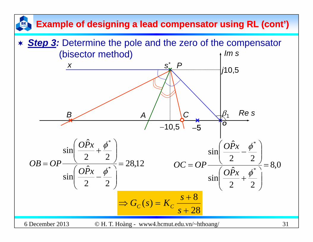
Example of designing a lead compensator using RL (cont’)Example of designing a lead compensator using RL (cont’)
Step 3: Determine the pole and the zero of the compensator Step 3: Determine the pole and the zero of the compensator(bisector method)
s* PxIm s
j10,5
1O
AB C Re s
510,5 5
12,28ˆ22
ˆsin
*
*
xPO
OPOB 0,822
ˆsin
*
xPO
OPOC,
22ˆ
sin*
xPO
0,8
22ˆ
sin*
xPO
OPOC
8s
6 December 2013 © H. T. Hoàng - www4.hcmut.edu.vn/~hthoang/ 31
288)(
ssKsG CC
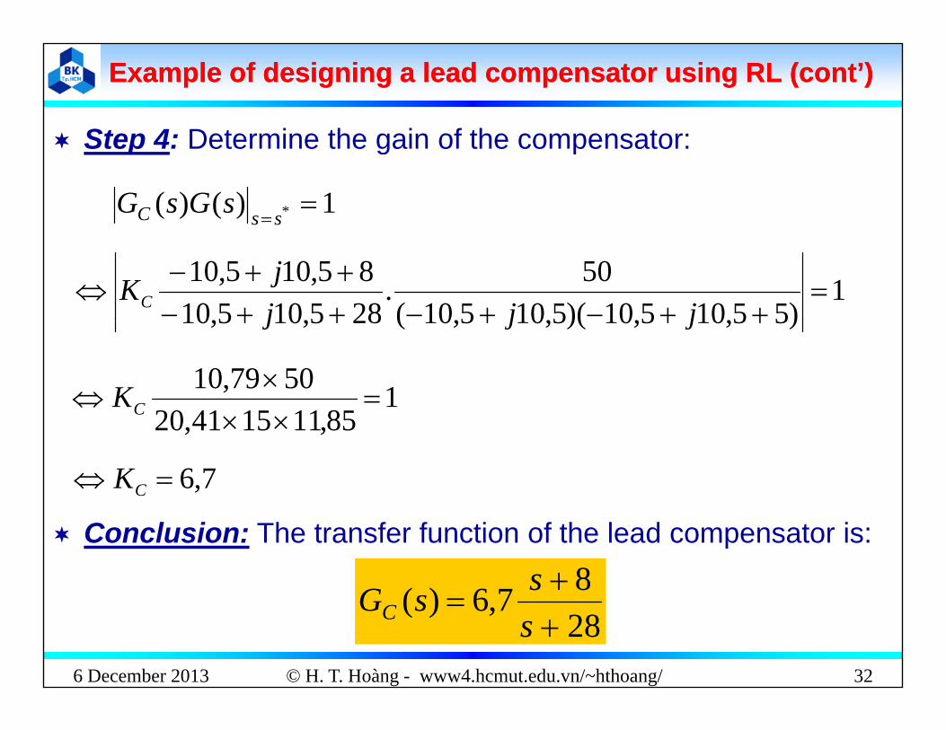
Example of designing a lead compensator using RL (cont’)Example of designing a lead compensator using RL (cont’)
Step 4: Determine the gain of the compensator: Step 4: Determine the gain of the compensator:
1)()( * ssC sGsG
1)5510510)(510510(
50.2851051085,105,10
jjjjKC )55,105,10)(5,105,10(285,105,10 jjj
18511154120
5079,10
CK
85,111541,20 C
7,6 CK
876)( sG
Conclusion: The transfer function of the lead compensator is:
6 December 2013 © H. T. Hoàng - www4.hcmut.edu.vn/~hthoang/ 32
287,6)(
ssGC

Root locus of the systemRoot locus of the system
Root locus of the Root locus of the
6 December 2013 © H. T. Hoàng - www4.hcmut.edu.vn/~hthoang/ 33
uncompensated system compensated system
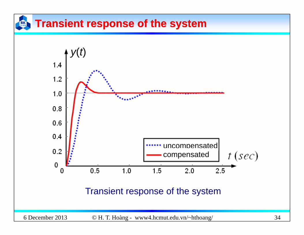
Transient response of the systemTransient response of the system
y(t)
uncompensatedcompensated
Transient response of the system
6 December 2013 © H. T. Hoàng - www4.hcmut.edu.vn/~hthoang/ 34
Transient response of the system

Procedure for designing lag compensator using the root locusProcedure for designing lag compensator using the root locus
)/1( Ts )1( )/1()/1()(
TsTsKsG CCLag compensator:
Step 1: Determine to meet the steady-state error requirement: Step 1: Determine to meet the steady-state error requirement:
*P
KK
*V
KK
*a
KK
or orPK VK aK
Step 2: Chose the zero of the lag compensator: )Re(1 *21s Step 2: Chose the zero of the lag compensator: )( 2,1T
11 Step 3: Calculate the pole of the compensator:
TT . Step 3: Calculate the pole of the compensator:
Step 4: Calculate K satisfying the condition: 1)()( * sGsG
6 December 2013 © H. T. Hoàng - www4.hcmut.edu.vn/~hthoang/ 35
Step 4: Calculate KC satisfying the condition: 1)()( *2,1
ssC sGsG

Example of designing a lag compensator using RLExample of designing a lag compensator using RL
( )R(s)+
Y(s)GC(s)
)4)(3(10
sss
Objective: design the compensator GC(s) so that the j g p C( )compensated system satisfies the following performances: steady state error to ramp input is 0,02 and transient response of the compensated system is nearly unchangedresponse of the compensated system is nearly unchanged.
Solution:
)1()/1()(
TsKsG
The compensator to be design is a lag compensator:
6 December 2013 © H. T. Hoàng - www4.hcmut.edu.vn/~hthoang/ 36
)1( )/1(
)(
Ts
KsG CC
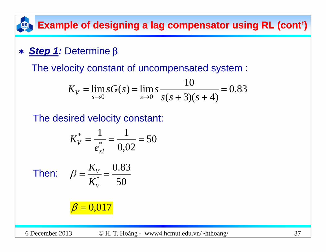
Example of designing a lag compensator using RL (cont’)Example of designing a lag compensator using RL (cont’)
Step 1: Determine
The velocity constant of uncompensated system :
83.0)4)(3(
10lim)(lim00
sss
sssGKssV
5011*
* VK
The desired velocity constant:
5002,0*
xlV e
K
83.0 VKThen:
50* VK
Then:
0170
6 December 2013 © H. T. Hoàng - www4.hcmut.edu.vn/~hthoang/ 37
017,0

Example of designing a lag compensator using RL (cont’)Example of designing a lag compensator using RL (cont’)
Step 2: Chose the zero of the lag compensator Step 2: Chose the zero of the lag compensatorThe pole of the uncompensated system:
10 1 js0)(1 sG 0)4)(3(
101
sss
51
3
2,1
sjs
Th d i t l f th t d t j1 The dominant poles of the uncompensated system: js 12,1
1Re11 s
TChose: 1,01
T
T T
Step 3: Calculate the pole of the compensator:11 1
)1,0)(017,0(11
TT 0017,01
T
1,0)(
sKsG
6 December 2013 © H. T. Hoàng - www4.hcmut.edu.vn/~hthoang/ 38
0017,0)(
sKsG CC
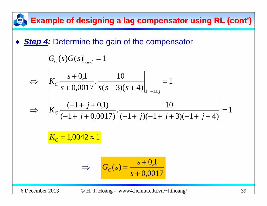
Example of designing a lag compensator using RL (cont’)Example of designing a lag compensator using RL (cont’)
Step 4: Determine the gain of the compensator
1)()( * ssC sGsGss
1)4)(3(
10.0017,0
1,0 1
jC ssss
sK))((7, 1 js
1)41)(31)(1(
10.)001701(
)1,01(
jjjjjKC )41)(31)(1()0017,01( jjjj
10042,1 CK
1,0)(
ssG
6 December 2013 © H. T. Hoàng - www4.hcmut.edu.vn/~hthoang/ 39
0017,0)(
ssGC
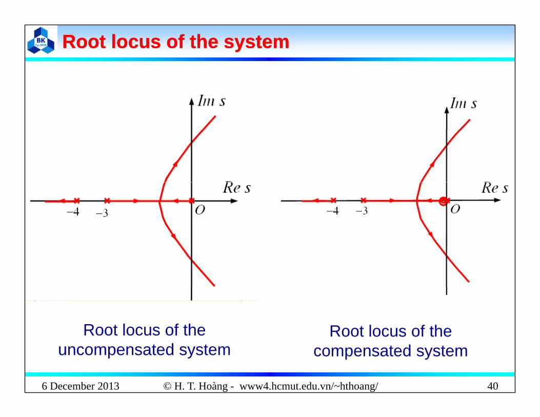
Root locus of the systemRoot locus of the system
Root locus of the Root locus of the
6 December 2013 © H. T. Hoàng - www4.hcmut.edu.vn/~hthoang/ 40
uncompensated system compensated system

Transient response of the systemTransient response of the system
( )y(t)
uncompensatedt dcompensated
6 December 2013 © H. T. Hoàng - www4.hcmut.edu.vn/~hthoang/ 41
Transient response of the system

Procedure for designing lead lag compensator using the RLProcedure for designing lead lag compensator using the RL
The compensator to be designed
)()()( 21 sGsGsG CCC
The compensator to be designed
phaselead
phaselag
Step 1: Design the lead compensator GC1(s) to satisfy thetransient response performances.
Step 2: Let G1(s)= G (s). GC1(s)D i h l G ( ) i i i h G ( )Design the lag compensator GC2(s) in series with G1(s) tosatisfy the steady-state performances (and not to degrade thetransient response obtained after phase lead compensating)
6 December 2013 © H. T. Hoàng - www4.hcmut.edu.vn/~hthoang/ 42
transient response obtained after phase lead compensating)
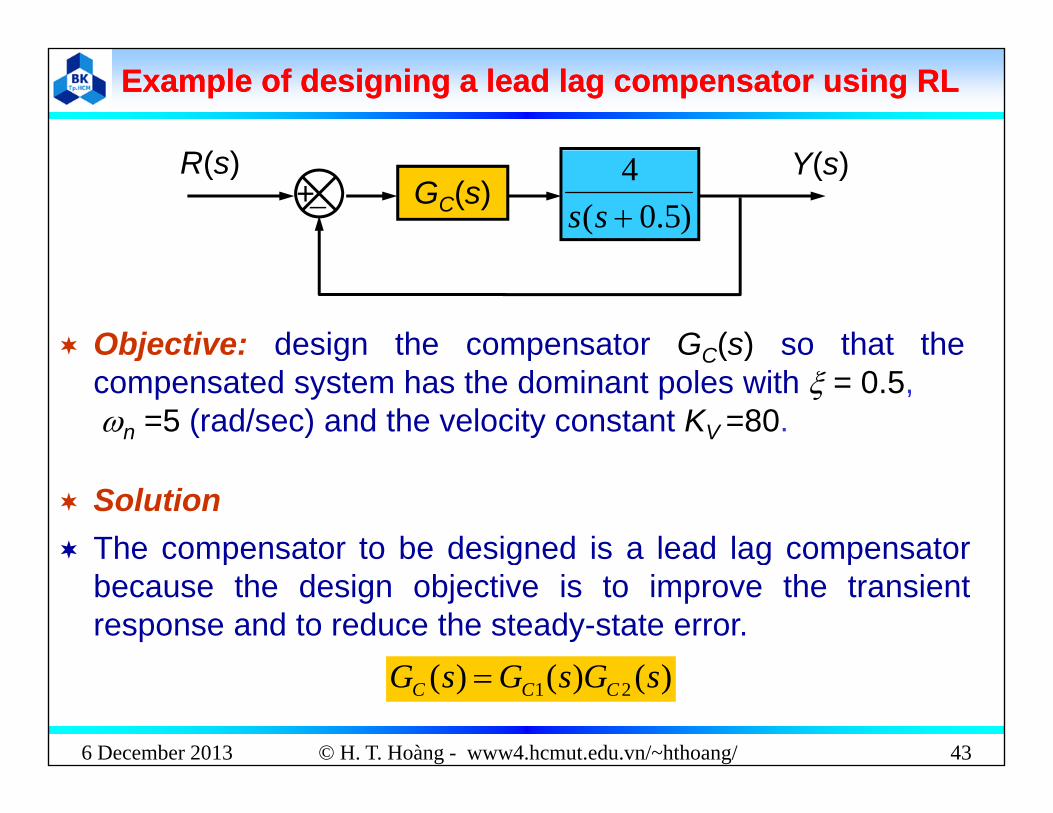
Example of designing a lead lag compensator using RLExample of designing a lead lag compensator using RL
( )R(s)+
Y(s)GC(s)
)5.0(4ss
Objective: design the compensator GC(s) so that thej g p C( )compensated system has the dominant poles with = 0.5,n =5 (rad/sec) and the velocity constant KV =80.
Solution The compensator to be designed is a lead lag compensatorp g g p
because the design objective is to improve the transientresponse and to reduce the steady-state error.
6 December 2013 © H. T. Hoàng - www4.hcmut.edu.vn/~hthoang/ 43
)()()( 21 sGsGsG CCC
Example of designing a lead lag compensator using RL (cont’)Example of designing a lead lag compensator using RL (cont’)
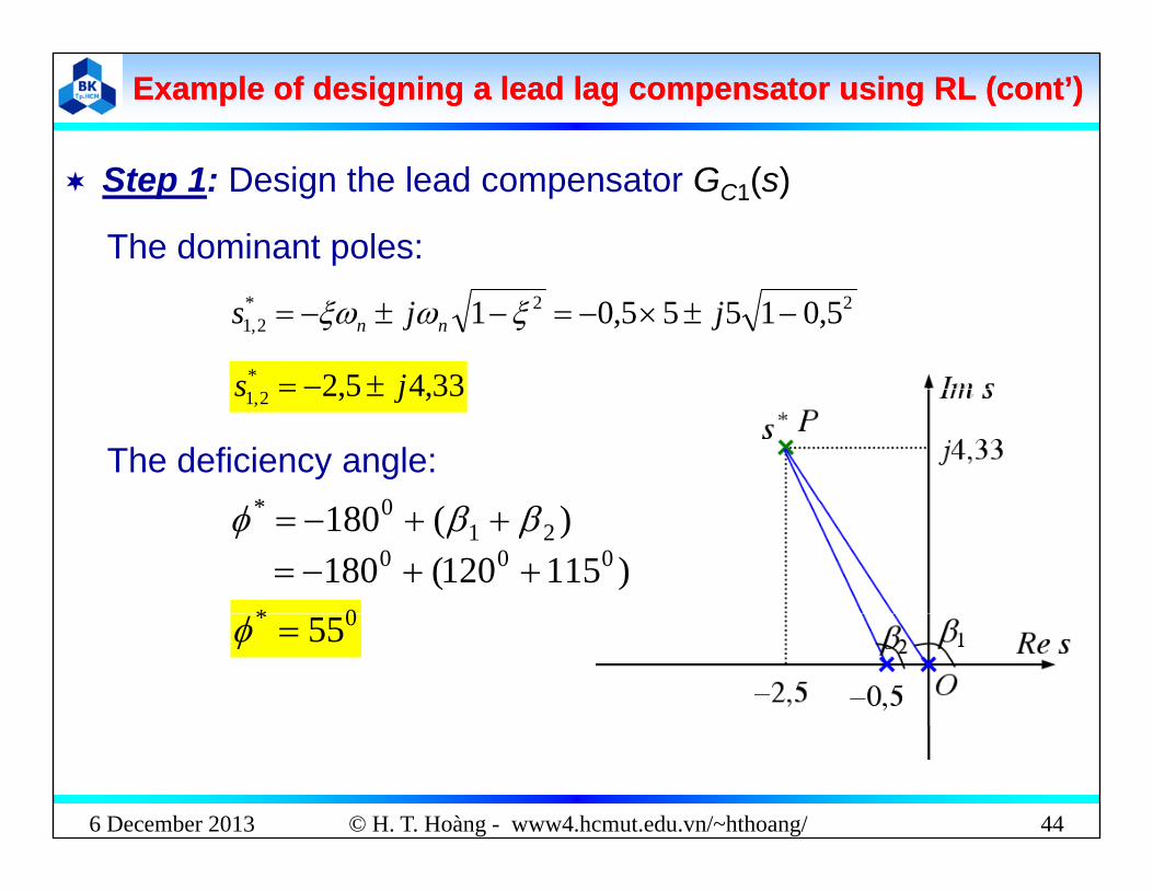
Step 1: Design the lead compensator GC1(s)
The dominant poles:22*
2,1 5,01555,01 jjs nn
33452* js 33,45,22,1 js
The deficiency angle:0* )(180 210*
)115120(180 000 0* 0* 55
6 December 2013 © H. T. Hoàng - www4.hcmut.edu.vn/~hthoang/ 44

Example of designing a lead lag compensator using RL (cont’)Example of designing a lead lag compensator using RL (cont’)
Chose the zero of the lead compensator so that it eliminatesChose the zero of the lead compensator so that it eliminatesthe pole at –0.5 of G(s) (pole elimination method)
501
5,01
T
5,0OA
5.460sin55sin76.4
sin
ˆsin0
0
PAB
BPAPAAB
5,0OA
AB51
1 ABOA
T–1/T1–1/T1
1
55,0)( 11
sKsG CC
6 December 2013 © H. T. Hoàng - www4.hcmut.edu.vn/~hthoang/ 45
5s

Example of designing a lead lag compensator using RL (cont’)Example of designing a lead lag compensator using RL (cont’)
C l l KCalculate KC1: 1)()( *1 ssC sGsG
145,0sK 1)5,0(
.5,
33,45,21
jsC sss
K
256K 25,61 CK
5,025,6)(1
ssGC
The lead-compensated open-loop system:
525,6)(1 s
sGC
)5(25)()()( 11
ss
sGsGsG C
The lead-compensated open-loop system:
6 December 2013 © H. T. Hoàng - www4.hcmut.edu.vn/~hthoang/ 46
)5( ss

Example of designing a lead lag compensator using RL (cont’)Example of designing a lead lag compensator using RL (cont’)
Step 2: Design the lag compensator GC2(s)1T
s
2
222 1)(
Ts
TKsG CC
2T Determine :
525lim)(lim 1 sssGKV 5)5(
lim)(lim010 sssssGK
ssV
80* VKV
161
805
* V
KK
6 December 2013 © H. T. Hoàng - www4.hcmut.edu.vn/~hthoang/ 47
1680VK

Example of designing a lead lag compensator using RL (cont’)Example of designing a lead lag compensator using RL (cont’)
D i h f h l Determine the zero of the lag compensator:
5,2)33,45,2Re()Re(1 * jsT 2T
16,01
Chose: ,
2T
)16,0.(1611.1
Calculate the pole of the lag compensator:
),(1622 TT
01.01
6 December 2013 © H. T. Hoàng - www4.hcmut.edu.vn/~hthoang/ 48
2T
Example of designing a lead lag compensator using RL (cont’)Example of designing a lead lag compensator using RL (cont’)
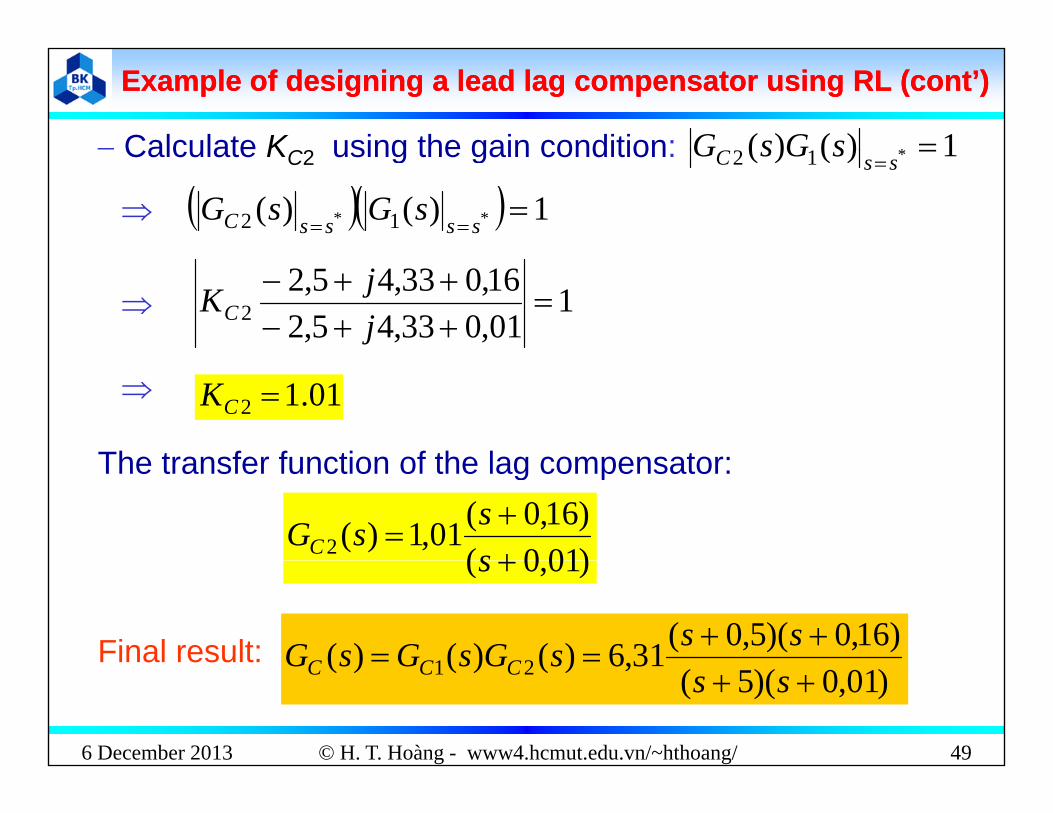
Calculate KC2 using the gain condition: 1)()( *12 C sGsGCalculate KC2 using the gain condition: 1)()( *12 ssC sGsG
1)()( ** 12 ssssC sGsG
101,033,45,216,033,45,2
2
jjKC
The transfer function of the lag compensator:
01.12 CK
)010()16,0(01,1)(2
sssGC
The transfer function of the lag compensator:
)16,0)(5,0(31,6)()()( 21
sssGsGsG CCCFinal result:
)01,0( s
6 December 2013 © H. T. Hoàng - www4.hcmut.edu.vn/~hthoang/ 49
)01,0)(5(31,6)()()( 21 ss
sGsGsG CCC
Control system Control system design in design in yy ggfrequency domainfrequency domain
6 December 2013 © H. T. Hoàng - www4.hcmut.edu.vn/~hthoang/ 50
Procedure for designing lead compensators in frequency domainProcedure for designing lead compensators in frequency domain
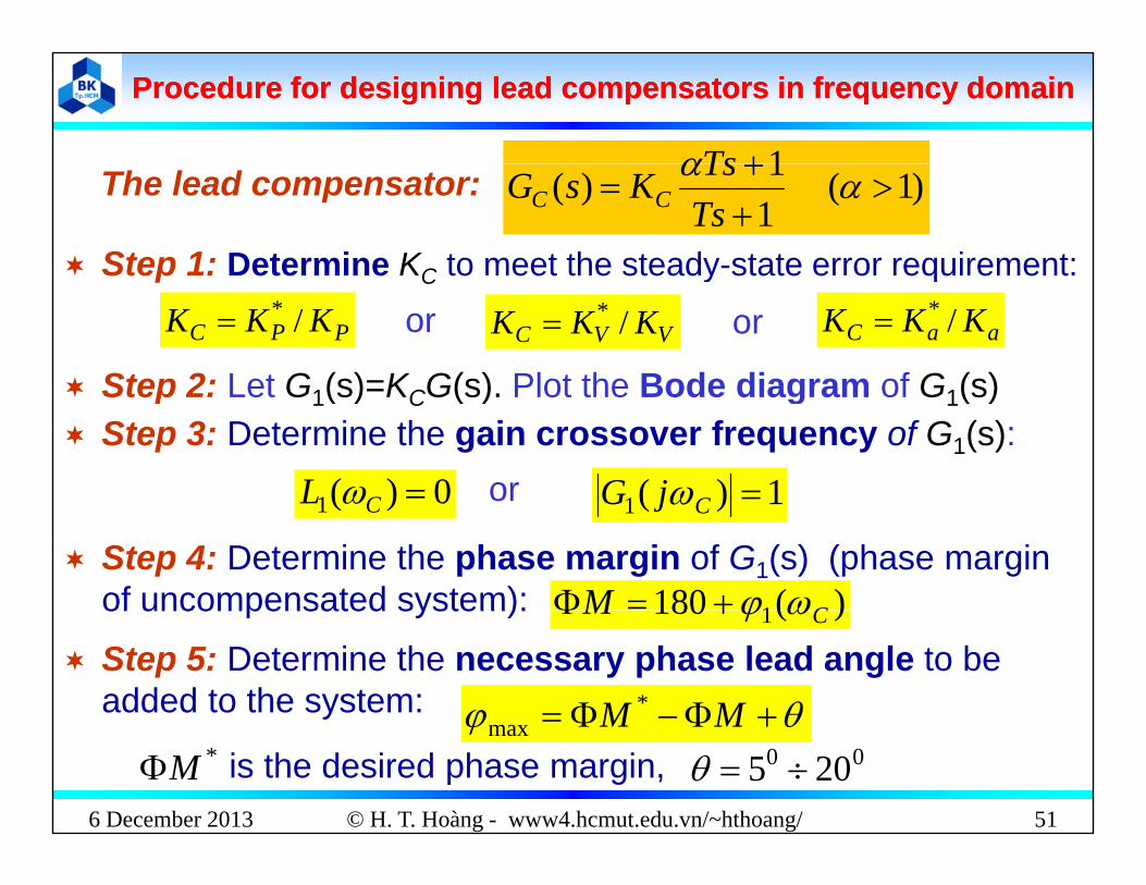
1Ts )1( 11)(
TsTsKsG CCThe lead compensator:
Step 1: Determine KC to meet the steady-state error requirement: Step 1: Determine KC to meet the steady state error requirement:
PPC KKK /* VVC KKK /* aaC KKK /*or or
Step 2: Let G (s)=K G(s) Plot the Bode diagram of G (s) Step 2: Let G1(s)=KCG(s). Plot the Bode diagram of G1(s) Step 3: Determine the gain crossover frequency of G1(s):
0)(1 CL 1)(1 CjG or0)(1 CL 1)(1 CjG or
Step 4: Determine the phase margin of G1(s) (phase margin of uncompensated system): )(180 1 CM of uncompensated system): )(180 1 CM
Step 5: Determine the necessary phase lead angle to be added to the system: MM *
6 December 2013 © H. T. Hoàng - www4.hcmut.edu.vn/~hthoang/ 51
MMmax
is the desired phase margin,*M 00 205

Procedure for designing lead compensators in frequency domainProcedure for designing lead compensators in frequency domain
sin1
St 7 D t i th i f ( f
Step 6: Calculate :max
max
sin1sin1
Step 7: Determine the new gain crossover frequency (ofthe compensated open-loop system) using the conditions:
lg10)(1 CL /1)( jGor lg10)(1 CL /1)(1 CjGor
Step 8: Calculate the time constant T: T 1pC
Step 9: Check if the compensated system satisfies the gainmargin? If not repeat the design procedure from step 5margin? If not, repeat the design procedure from step 5.
Note: It is possible to determine C (step 3), M (step 4) and’C (step 7) by using Bode diagram instead of using analytic
6 December 2013 © H. T. Hoàng - www4.hcmut.edu.vn/~hthoang/ 52
C (step 7) by using Bode diagram instead of using analyticcalculation.
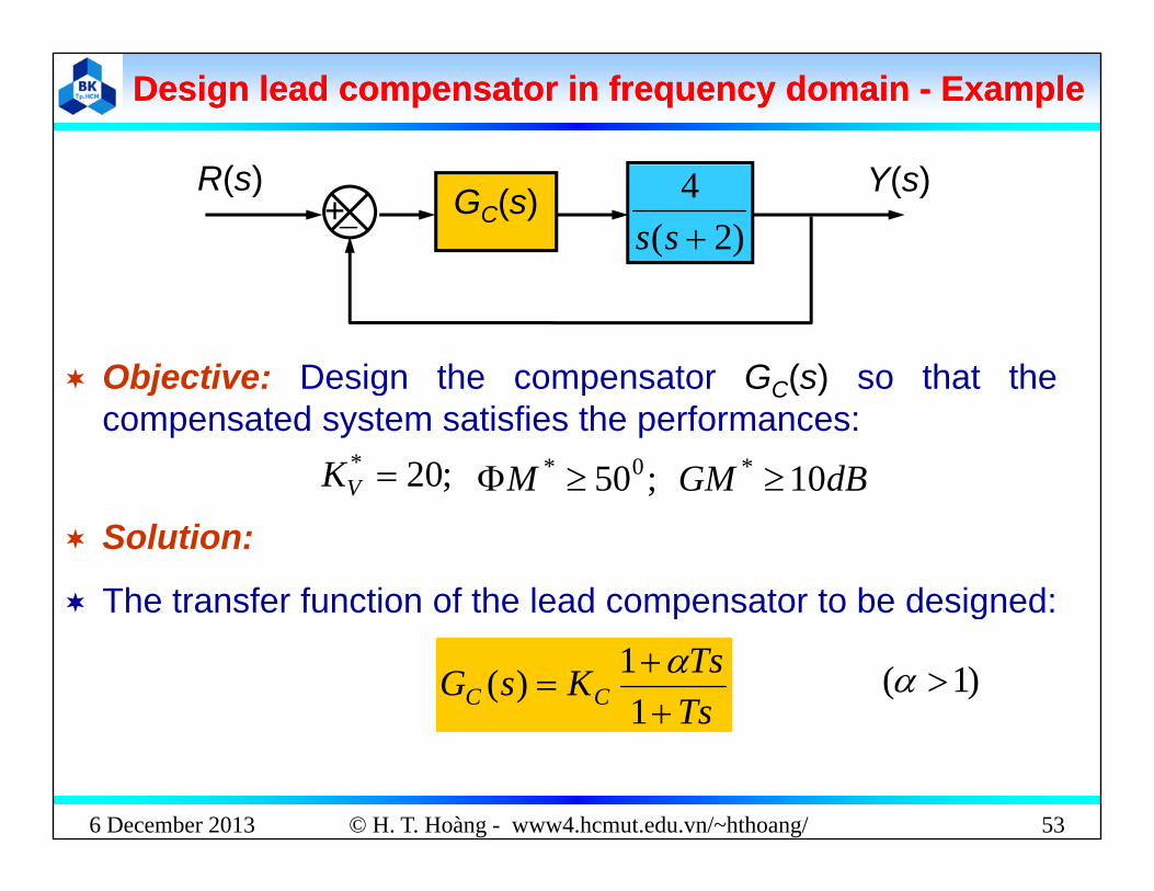
Design lead compensator in frequency domain Design lead compensator in frequency domain -- ExampleExample
( )R(s)+
Y(s)GC(s))2(
4ss
Objective: Design the compensator GC(s) so that thej g p C( )compensated system satisfies the performances:
;20* VK ;500* M dBGM 10*
Solution:
The transfer function of the lead compensator to be designed:p g
TsTsKsG CC
11)( )1(
6 December 2013 © H. T. Hoàng - www4.hcmut.edu.vn/~hthoang/ 53

Design lead compensator in frequency domain Design lead compensator in frequency domain –– Example (cont’)Example (cont’)
Step 1: Determine K Step 1: Determine KC
The velocity constant of the uncompensated system:
24li)(li GK 2)2(
lim)(lim00
ss
sssGKssV
The desired velocity constant: 20* VK
220*
V
VC K
KK 10CK
y V
V
Step 2: Denote)2(
4.10)()(1
sssGKsG C
)15,0(20)(1
ss
sG
6 December 2013 © H. T. Hoàng - www4.hcmut.edu.vn/~hthoang/ 54
Draw the Bode diagram of G1(s)

Design lead compensator in frequency domain Design lead compensator in frequency domain –– Example (cont’)Example (cont’)
-20dB/dec26
-40dB/dec
c=62
160
M
6 December 2013 © H. T. Hoàng - www4.hcmut.edu.vn/~hthoang/ 55
-160
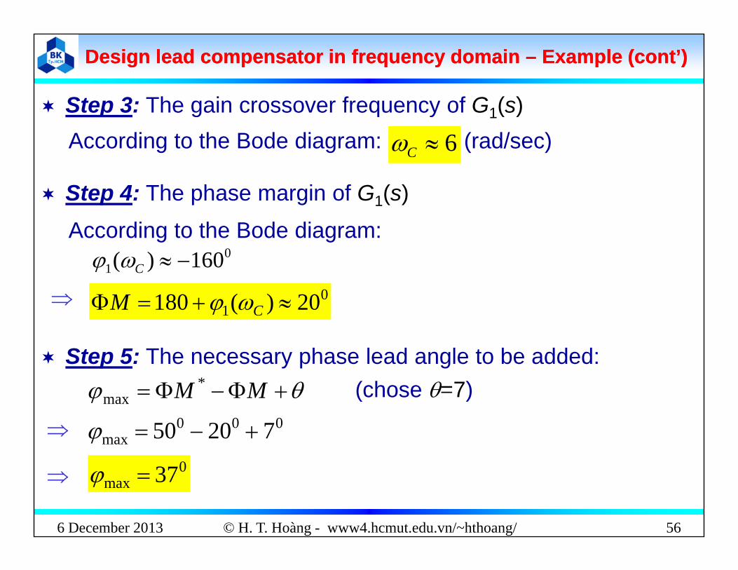
Design lead compensator in frequency domain Design lead compensator in frequency domain –– Example (cont’)Example (cont’)
Step 3: The gain crossover frequency of G (s) Step 3: The gain crossover frequency of G1(s)According to the Bode diagram: 6C (rad/sec)
Step 4: The phase margin of G1(s)
According to the Bode diagram:00
1 160)( C0
1 20)(180 CM
Step 5: The necessary phase lead angle to be added: MM * (chose =7)
000max 72050
0
MMmax (chose 7)
6 December 2013 © H. T. Hoàng - www4.hcmut.edu.vn/~hthoang/ 56
0max 37

Design lead compensator in frequency domain Design lead compensator in frequency domain –– Example (cont’)Example (cont’)
Step 6: Calculate Step 6: Calculate
0
0max
37sin137sin1
sin1sin1
4
Step 7: Determine the new gain crossover frequency using Bode plot
max 37sin1sin1
dBL 64lg10lg10)( p dBL C 64lg10lg10)(1
The abscissa of the intersection between Bode magnitudediagram and the horizontal line with ordinate of 6dB is thed ag a a d e o o a e o d a e o 6d s enew gain crossover frequency. According to the plot (in slide54), we have:
9C (rad/sec)9C (rad/sec) Step 8: Calculate T
11T
6 December 2013 © H. T. Hoàng - www4.hcmut.edu.vn/~hthoang/ 57
)4)(9(
C
T 056,0T 224,0T
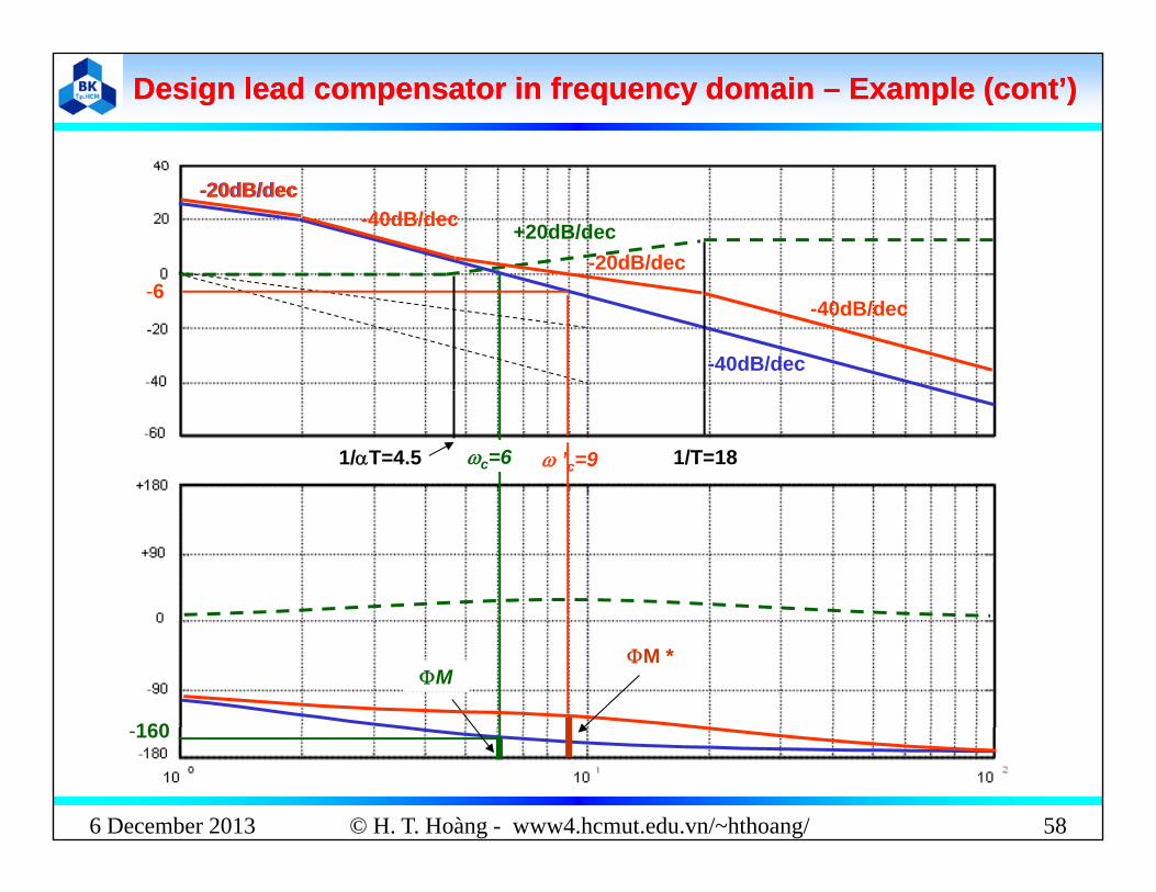
Design lead compensator in frequency domain Design lead compensator in frequency domain –– Example (cont’)Example (cont’)
-20dB/dec
+20dB/dec
-20dB/dec-40dB/dec
-20dB/dec
-40dB/dec
-6-40dB/dec
c=6 ’c=9 1/T=181/T=4.5
160
MM *
6 December 2013 © H. T. Hoàng - www4.hcmut.edu.vn/~hthoang/ 58
-160
Design lead compensator in frequency domain Design lead compensator in frequency domain –– Example (cont’)Example (cont’)
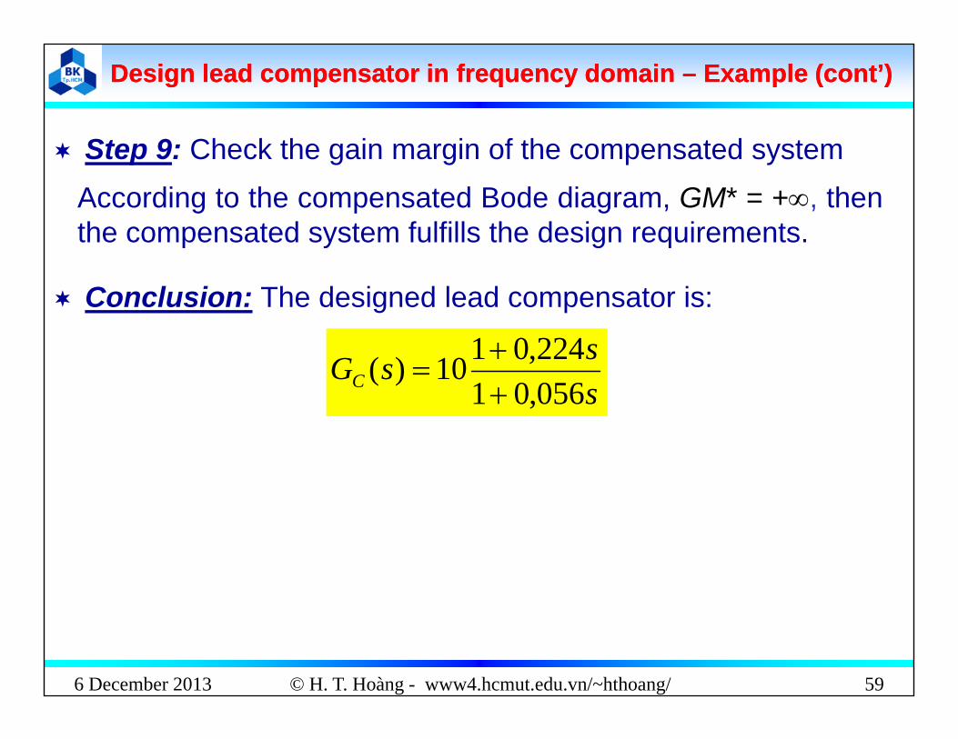
Step 9: Check the gain margin of the compensated system
According to the compensated Bode diagram, GM* = +, thenthe compensated system fulfills the design requirementsthe compensated system fulfills the design requirements.
Conclusion: The designed lead compensator is:
sssGC 056,01
224,0110)(
6 December 2013 © H. T. Hoàng - www4.hcmut.edu.vn/~hthoang/ 59

Design lead compensator in frequency Design lead compensator in frequency domain domain –– Example 2Example 2
( )R(s)+
Y(s)GC(s) G(s)
16)(02.0eG
s
Objective: Design the compensator G (s) so that the
)2510)(2()( 2
ssssG
Objective: Design the compensator GC(s) so that thecompensated system has: andsteady-state error to unit step input ;05.0* sse
;500* M dBGM 10* steady state error to unit step input ;05.0sse
Solution:
6 December 2013 © H. T. Hoàng - www4.hcmut.edu.vn/~hthoang/ 60

Procedure for designing lag compensators in frequency domainProcedure for designing lag compensators in frequency domain
1Ts )1( 11)(
TsTsKsG CCThe lag compensator:
Step 1: Determine KC to meet the steady-state error requirement: Step 1: Determine KC to meet the steady state error requirement:
PPC KKK /* VVC KKK /* aaC KKK /*or or
Step 2: Let G (s)=K G(s) Plot the Bode diagram of G (s) Step 2: Let G1(s)=KCG(s). Plot the Bode diagram of G1(s) Step 3: Determine the new gain crossover frequency
satisfying the following condition:C
satisfying the following condition:
is the desired phase margin*M 00 205 *0
1 180)( MC
is the desired phase margin,M 205 Step 4: Calculate using the condition:
l20)( L 1)( jGor
6 December 2013 © H. T. Hoàng - www4.hcmut.edu.vn/~hthoang/ 61
lg20)(1 CL
)(1 CjGor

Procedure for designing lag compensators in frequency domainProcedure for designing lag compensators in frequency domain
St 5 Ch th f th l t th t Step 5 : Chose the zero of the lag compensator so that:
CT
1 TT
Step 6: Calculate the time constant T:
TT 11
T
Step 7: Check if the compensated system satisfies the gainmargin? If not, repeat the design procedure from step 3.
Note: It is possible to determine , (step 3), (step 4) by using Bode diagram instead of using analytic
C)(1 C )(1 CL
6 December 2013 © H. T. Hoàng - www4.hcmut.edu.vn/~hthoang/ 62
calculation.

Design lag compensator in frequency domain Design lag compensator in frequency domain –– ExampleExample
( )R(s)+
Y(s)GC(s))15.0)(1(
1 sss
Objective: design the lag compensator GC(s) so that thatj g g p C( )compensated system satisfies the following performances:
;5* VK ;400* M dBGM 10*
Solution The transfer function of the lag compensator to be designed: The transfer function of the lag compensator to be designed:
TsTsKsG CC
11)( )1(
6 December 2013 © H. T. Hoàng - www4.hcmut.edu.vn/~hthoang/ 63
Ts1

Design lag compensator in frequency domain Design lag compensator in frequency domain –– Example (cont’)Example (cont’)
Step 1: Determine KC Step 1: Determine KC
The velocity constant of the uncompensated system:
11lim)(lim GK 1)15.0)(1(
lim)(lim00
sss
sssGKssV
The desired velocity constant: 5* VK
5*
V
VC K
KK
y V
V
Step 2: Denote )()(1 sGKsG C5
)15.0)(1(
5)(1
ssssG
6 December 2013 © H. T. Hoàng - www4.hcmut.edu.vn/~hthoang/ 64
Draw the Bode diagram of G1(s)
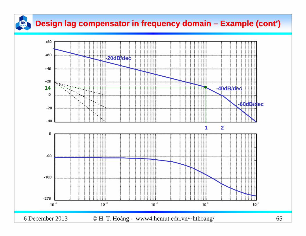
Design lag compensator in frequency domain Design lag compensator in frequency domain –– Example (cont’)Example (cont’)
-20dB/dec
60dB/dec
-40dB/dec14
-60dB/dec
21
6 December 2013 © H. T. Hoàng - www4.hcmut.edu.vn/~hthoang/ 65

Design lag compensator in frequency domain Design lag compensator in frequency domain –– Example (cont’)Example (cont’)
Step 3: Determine the new gain crossover frequency:
*01 180)( MC
01 135)( C
0001 540180)( C
According to the Bode diagram: 5.0C (rad/sec)
St 4 C l l t i th diti
1 135)( C
Step 4: Calculate using the condition: lg20)(1 CL
( )According the Bode diagram: (dB)18)(1 CL lg2018 9,0lg 9,010
6 December 2013 © H. T. Hoàng - www4.hcmut.edu.vn/~hthoang/ 66
126,0
Design lag compensator in frequency domain Design lag compensator in frequency domain –– Example (cont’)Example (cont’)
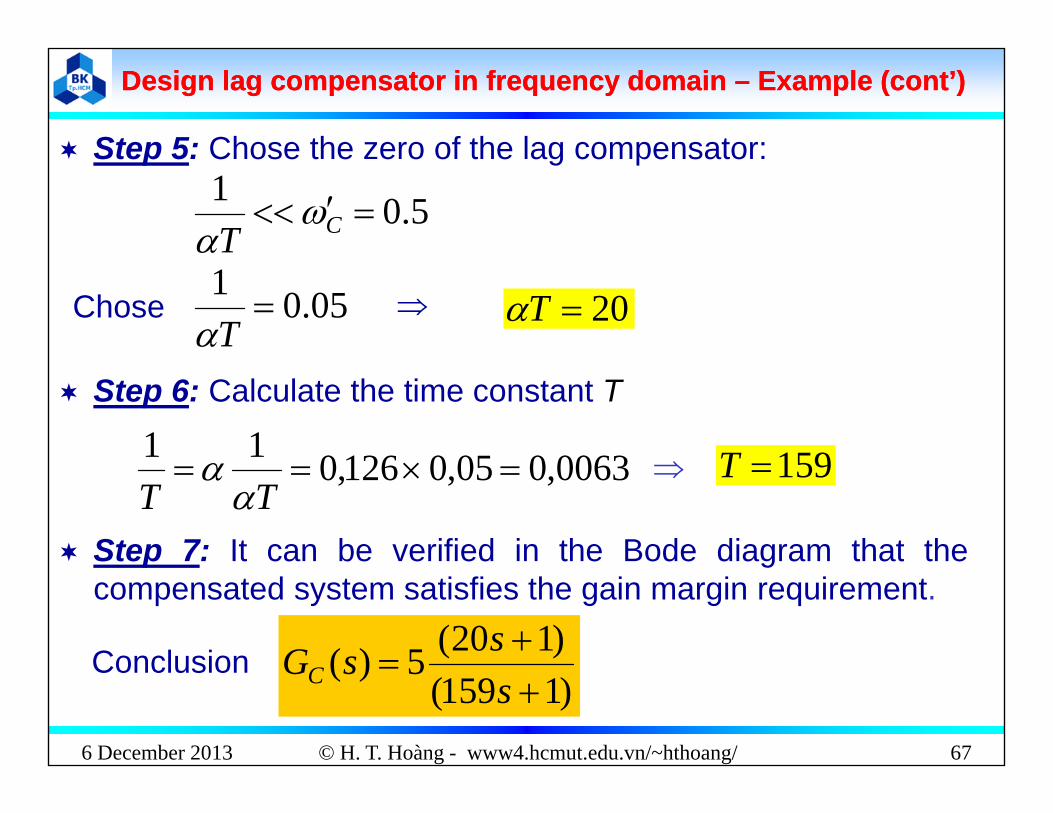
Step 5: Chose the zero of the lag compensator: Step 5: Chose the zero of the lag compensator:
5.01 CT
Chose 05.01
T 20T
159T
Step 6: Calculate the time constant T
00630050126011 159T0063,005,0126,0
TT
Step 7: It can be verified in the Bode diagram that the Step 7: It can be verified in the Bode diagram that thecompensated system satisfies the gain margin requirement.
)120(5)(
ssGConclusion
6 December 2013 © H. T. Hoàng - www4.hcmut.edu.vn/~hthoang/ 67
)1159(5)(
ssGCConclusion
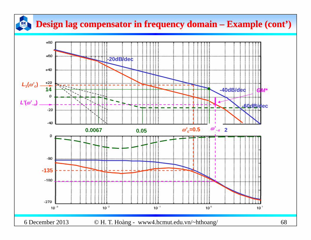
Design lag compensator in frequency domain Design lag compensator in frequency domain –– Example (cont’)Example (cont’)
-20dB/dec
60dB/dec
-40dB/dec14L1(’c)
L’(’)
GM*
-60dB/dec
21’c=0.50.0067 0.05 ’
( )
-135
6 December 2013 © H. T. Hoàng - www4.hcmut.edu.vn/~hthoang/ 68

Design lag Design lag compensator in frequency compensator in frequency domain domain –– Example 2Example 2
( )R(s)+
Y(s)GC(s) G(s)
16)(02.0eG
s
Objective: Design the compensator G (s) so that the
)2510)(2()( 2
ssssG
Objective: Design the compensator GC(s) so that thecompensated system has: andsteady-state error to unit step input ;05.0* sse
;500* M dBGM 10* steady state error to unit step input ;05.0sse
Solution:
6 December 2013 © H. T. Hoàng - www4.hcmut.edu.vn/~hthoang/ 69

Comparison of phase lead and phase lag compensatorComparison of phase lead and phase lag compensator
6 December 2013 © H. T. Hoàng - www4.hcmut.edu.vn/~hthoang/ 70
(Dorf and Bishop (2008), Modern control system –p.729)

D i f PIDD i f PID t llt llDesign of PID Design of PID controllers controllers
6 December 2013 © H. T. Hoàng - www4.hcmut.edu.vn/~hthoang/ 71

Zeigler Zeigler Nichols method 1Nichols method 1
Determine the PID parameters based on the step response of Determine the PID parameters based on the step response ofthe open-loop system.
Plantu(t) y(t)
y(t)
K
t
6 December 2013 © H. T. Hoàng - www4.hcmut.edu.vn/~hthoang/ 72
T1 T2
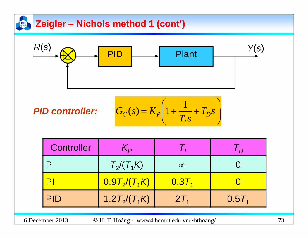
Zeigler Zeigler Nichols method 1 (cont’) Nichols method 1 (cont’)
R( )R(s)+
Y(s)PlantPID
1PID controller:
sT
sTKsG D
IPC
11)(
Controller KP TI TD
P T /(T K) 0P T2/(T1K) 0
PI 0.9T2/(T1K) 0.3T1 0
6 December 2013 © H. T. Hoàng - www4.hcmut.edu.vn/~hthoang/ 73
PID 1.2T2/(T1K) 2T1 0.5T1

Zeigler Zeigler Nichols method 1 Nichols method 1 –– Example Example
Problem: Design a PID y(t) Problem: Design a PID controller to control a furnace providing the open-loop h t i ti f th f
y(t)
characteristic of the furnace obtained from a experiment beside.
150
t (min)( )
8 24150K
sec480min81 T
024014402121 2 TKP
ssGPID 240110240)(
sec1440min242 T
024.0150480
2.12.11 KT
KP
sec96048022 1 TTI
ss
sGPID 240960
1024.0)(
6 December 2013 © H. T. Hoàng - www4.hcmut.edu.vn/~hthoang/ 74
sec2404805.05.0 1 TTD

Zeigler Zeigler Nichols method 2Nichols method 2 Determine the PID parameters based on the response of the Determine the PID parameters based on the response of the
closed-loop system at the stability boundary.
Plant+ KKcr
y(t)
Tcr
6 December 2013 © H. T. Hoàng - www4.hcmut.edu.vn/~hthoang/ 75
t

Zeigler Zeigler Nichols method 2 (cont’)Nichols method 2 (cont’)
R(s)+
Y(s)PlantPID
1PID controller:
sT
sTKsG D
IPC
11)(
Controller KP TI TD
P 0 5K 0P 0.5Kcr 0
PI 0.45Kcr 0.83Tcr 0
6 December 2013 © H. T. Hoàng - www4.hcmut.edu.vn/~hthoang/ 76
PID 0.6Kcr 0.5Tcr 0.125Tcr
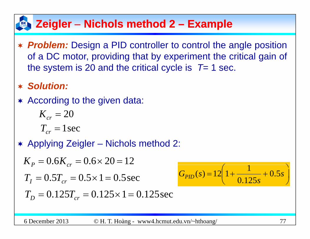
Zeigler Zeigler Nichols method 2 Nichols method 2 –– ExampleExample
Problem: Design a PID controller to control the angle position Problem: Design a PID controller to control the angle positionof a DC motor, providing that by experiment the critical gain ofthe system is 20 and the critical cycle is T= 1 sec.
According to the given data: Solution:
20crKsec1crT
g g
Applying Zeigler – Nichols method 2:
12206.06.0 crP KK
s
ssGPID 5.0
125.01112)(
crP
sec5.015.05.0 crI TTsec1250112501250 TT
6 December 2013 © H. T. Hoàng - www4.hcmut.edu.vn/~hthoang/ 77
sec125.01125.0125.0 crD TT
Analytical method for designing PID controller Analytical method for designing PID controller
St 1 E t bli h ti ( ) ti th l ti hi Step 1: Establish equation(s) representing the relationship between the controller to be designed and the desired performances.
Step 2: Solve the equation(s) obtained in step 1 for the t ( ) f th t llparameter(s) of the controller.
6 December 2013 © H. T. Hoàng - www4.hcmut.edu.vn/~hthoang/ 78

Analytical method for designing PID controller Analytical method for designing PID controller
Example: Design PID controller so that the control system Example: Design PID controller so that the control system satisfies the following requirements: Closed-loop complex poles with =0.5 and n=8. Velocity constant KV = 100.
R(s) Y(s)100( )+
( )GPID(s)
10010100
2 ss
Solution: The transfer function of the PID controller to be Solution: The transfer function of the PID controller to be designed
sKKKsG DI
PC )(
6 December 2013 © H. T. Hoàng - www4.hcmut.edu.vn/~hthoang/ 79
sKs
KsG DPC )(
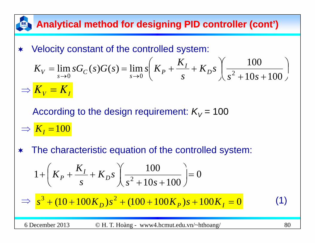
Analytical method for designing PID controller (cont’)Analytical method for designing PID controller (cont’)
Velocity constant of the controlled system:
10010100lim)()(lim 200 ss
sKs
KKssGssGK DI
PsCsV 1001000 sssss
IV KK
According to the design requirement: KV = 100
100IK
The characteristic equation of the controlled system:
100 K 010010
1001 2
sssK
sKK D
IP
0100)100100()10010( 23 KKK (1)
6 December 2013 © H. T. Hoàng - www4.hcmut.edu.vn/~hthoang/ 80
0100)100100()10010( 23 IPD KsKsKs (1)

Analytical method for designing PID controller (cont’)Analytical method for designing PID controller (cont’)
The desired characteristic equation: The desired characteristic equation:
0)2)(( 22 nnssas
0)648)(( 2 0)648)(( 2 ssas
064)648()8( 23 asasas (2)
Balancing the coefficients of the equations (1) and (2), we have:
aK 810010 25156
aKaK
aK
P
D
64100648100100
810010
54114,1225.156
P
KKa
aKI 64100 54,1DK
Conclusion: G 5411006412)(
6 December 2013 © H. T. Hoàng - www4.hcmut.edu.vn/~hthoang/ 81
Conclusion: ss
sGC 54,164,12)(
Manual tuning of PID controllersManual tuning of PID controllers
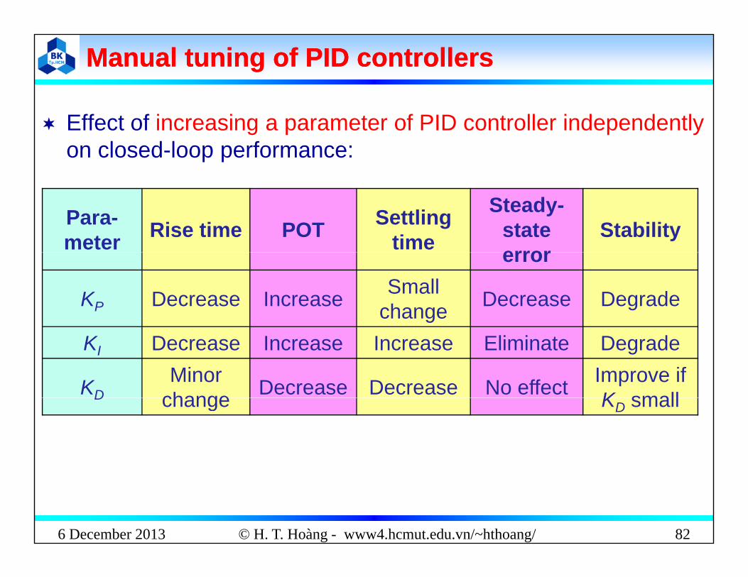
Effect of increasing a parameter of PID controller independently on closed-loop performance:
Para-meter Rise time POT Settling
time
Steady-stateerror
Stabilityerror
KP Decrease Increase Smallchange Decrease Degrade
KI Decrease Increase Increase Eliminate Degrade
KDMinor
change Decrease Decrease No effect Improve ifK smallD change KD small
6 December 2013 82© H. T. Hoàng - www4.hcmut.edu.vn/~hthoang/

A d f l t i f PID t ll
Manual tuning of PID controllers (cont.)Manual tuning of PID controllers (cont.)
A procedure for manual tuning of PID controllers:
1. Set KI and KD to 0, gradually increase KP to the critical i K (i th i k th l d l tgain Kcr (i.e. the gain makes the closed-loop system
oscilate)
2. Set KP Kcr /2
3. Gradually increase KI until the steady-state error is eliminated in a sufficient time for the process (Note that too much KI will cause instability).
4. Increase KD if needed to reduce POT and settling time (Note that too much KD will cause excessive response and overshoot)
6 December 2013 83© H. T. Hoàng - www4.hcmut.edu.vn/~hthoang/
Control systems design in stateControl systems design in state--spacespaceusing pole placement methodusing pole placement method
6 December 2013 © H. T. Hoàng - www4.hcmut.edu.vn/~hthoang/ 84
ControllabilityControllability
)()()( tutt BAxxC id t
)()()()()(
ttytutt
CxBAxx
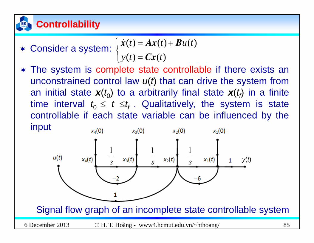
Consider a system:
The system is complete state controllable if there exists anunconstrained control law u(t) that can drive the system froman initial state x(t0) to a arbitrarily final state x(tf) in a finitetime interval t0 t tf . Qualitatively, the system is statetime interval t0 t tf . Qualitatively, the system is statecontrollable if each state variable can be influenced by theinput.
y(t)
6 December 2013 © H. T. Hoàng - www4.hcmut.edu.vn/~hthoang/ 85
Signal flow graph of an incomplete state controllable system

Controllability conditionControllability condition
)()()( ttt BAxx
)()()()()(
ttytutt
CxBAxx
System:
Controllability matrix
][ 12 BABAABB nC ][ BABAABB C
The necessary and sufficient condition for the controllability is:
nrank )(C
N t th t “ t ll bl ” i t d f “ l t Note: we use the term “controllable” instead of “complete state controllable” for short.
6 December 2013 © H. T. Hoàng - www4.hcmut.edu.vn/~hthoang/ 86

Controllability Controllability –– ExampleExample
)()()( tutt BAxx
)()()()()(
ttytutt
CxBAxx
Consider a system
where: 10 5where:
3210
A
25
B 31C
E l h ll bili f h
Solution: Controllability matrix:
Evaluate the controllability of the system.
ABBC Because:
162
25
C
Because:
84)det( C 2)( Crank
6 December 2013 © H. T. Hoàng - www4.hcmut.edu.vn/~hthoang/ 87
The system is controllable

State feedback controlState feedback controlr(t) u(t) y(t)x(t)
+r(t) u(t)
C y(t))()()( tutt BAxx
x(t)
K
Consider a system described by the state equations:
)()()()()(
ttytutt
CxBAxx
Consider a system described by the state equations:
The state feedback controller: )()()( ttrtu Kx )()( tty Cx
)()(][)( trtt BxBKAx
The state equations of the closed-loop system:
6 December 2013 © H. T. Hoàng - www4.hcmut.edu.vn/~hthoang/ 88
)() ty(t Cx

Pole placement methodPole placement method
If the system is controllable then it is possible to determineIf the system is controllable, then it is possible to determinethe feedback gain K so that the closed-loop system has thepoles at any location.
Step 1: Write the characteristic equation of the closed-loopsystem 0]det[ BKAIs (1)0]det[ BKAIs ( )
Step 2: Write the desired characteristic equation:n
0)(1
n
iips
)1( nip th d i d l
(2)
Step 3: Balance the coefficients of the equations (1) and (2),
),1( , nipi are the desired poles
6 December 2013 © H. T. Hoàng - www4.hcmut.edu.vn/~hthoang/ 89
we can find the state feedback gain K.

Pole placement method Pole placement method –– ExampleExample
Problem: Given a system described by the state state Problem: Given a system described by the state-state equation:
)()()( tutt BAxx
)()( tty Cx
010 0 100C
100010
A
30
B 374 1
Determine the state feedback controller )()()( ttrtu Kx Determine the state feedback controller so that the closed-loop system has complex poles with
and the third pole at 20. 10;6,0 n
)()()( ttrtu Kx
6 December 2013 © H. T. Hoàng - www4.hcmut.edu.vn/~hthoang/ 90
n

Pole placement method Pole placement method –– Example (cont’)Example (cont’)
Solution
The characteristic equation of the closed-loop system:0]det[ BKAIs
Solution
0]det[ BKAIs
030
100010
010001
d t
kkk 013
374100
100010det 321
kkks
The desired characteristic equation:
(1)0)12104()211037()33( 313212
323 kkskkkskks
The desired characteristic equation:
0)2)(20( 22 nnsss (2)23
6 December 2013 © H. T. Hoàng - www4.hcmut.edu.vn/~hthoang/ 91
(2)0200034032 23 sss

Pole placement method Pole placement method –– Example (cont’)Example (cont’)
B l th ffi i t f th ti (1) d (2) h Balance the coefficients of the equations (1) and (2), we have:
3233 32 kk
200012104340211037
21
321
kkkkk
Solve the above set of equations, we have:
578220k
48217839,3
578,220
2
1
kkk
482,173k
482178393578220K Conclusion:
6 December 2013 © H. T. Hoàng - www4.hcmut.edu.vn/~hthoang/ 92
482,17839,3578,220K Conclusion:
D i f t t ti tD i f t t ti tDesign of state estimatorsDesign of state estimators
6 December 2013 © H. T. Hoàng - www4.hcmut.edu.vn/~hthoang/ 93
The concept of state estimationThe concept of state estimation
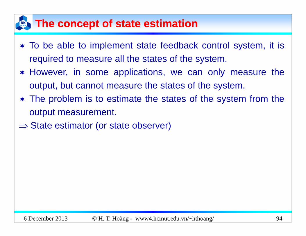
To be able to implement state feedback control system it is To be able to implement state feedback control system, it isrequired to measure all the states of the system.
However in some applications we can only measure the However, in some applications, we can only measure theoutput, but cannot measure the states of the system.
The problem is to estimate the states of the system from thep youtput measurement.
State estimator (or state observer)
6 December 2013 © H. T. Hoàng - www4.hcmut.edu.vn/~hthoang/ 94

ObservabilityObservability
)()()( tutt BAxx
)()()()()(
ttytutt
CxBAxx
Consider a system:
The system is complete state observable if given the control y p glaw u(t) and the output signal y(t) in a finite time interval t0 t tf , it is possible to determine the initial states x(t0). Qualitatively the system is state observable if all state variableQualitatively, the system is state observable if all state variable x(t) influences the output y(t).
y(t)
6 December 2013 © H. T. Hoàng - www4.hcmut.edu.vn/~hthoang/ 95
Signal flow graph of an incomplete state observable system
Observability conditionObservability condition
)()()( tutt BAxxS t
)()()()()(
ttytutt
CxBAxx System
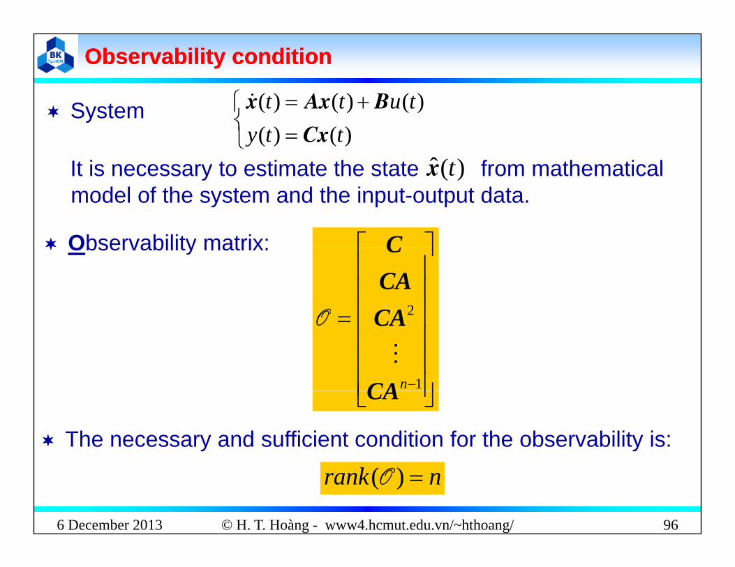
It is necessary to estimate the state from mathematical )(ˆ tx
Observability matrix: C
ymodel of the system and the input-output data.
)(
Observability matrix:
2CACAC
O
1nCA
CA
O
CA
The necessary and sufficient condition for the observability is:
6 December 2013 © H. T. Hoàng - www4.hcmut.edu.vn/~hthoang/ 96
nrank )(O

Observability Observability –– ExampleExample
)()()( tutt BAxx
)()()()()(
ttytutt
CxBAxx
Consider the system
10 1where:
32
10A
21
B 31C
Solution: Observability matrix:
Evaluate the observability of the system.
CAC
O
8
36
1O
Because 10)det( O 2)( Orank
6 December 2013 © H. T. Hoàng - www4.hcmut.edu.vn/~hthoang/ 97
The system is observable

State estimatorState estimator
u(t) y(t)x(t)r(t) u(t) y(t))()()( tutt BAxx x(t)
C
+
r(t)
CB
L)(ˆ tx
+++ C
)(ˆ tyB
A
+
K
)(ˆ)(ˆ))(ˆ)(()()(ˆ)(ˆ
ttytytytutt
xCLBxAx State estimator:
6 December 2013 © H. T. Hoàng - www4.hcmut.edu.vn/~hthoang/ 98
yT
nlll ][ 21 Lwhere:

Design of state estimatorsDesign of state estimators Requirements: Requirements:
The state estimator must be stable, estimation errorshould approach to zero.
Dynamic response of the state estimator should be fast Dynamic response of the state estimator should be fastenough in comparison with the dynamic response of thecontrol loop.
All the roots of the equation locates i th h lf l ft l
It is required to chose L satisfying:0)det( LCAsI
in the half-left s-plane. The roots of the equation are further
from the imaginary axis than the roots of the equation0)det( LCAsI
0)det( BKAsI Depending on the design of L, we have different state estimator:
Luenberger state observer
6 December 2013 © H. T. Hoàng - www4.hcmut.edu.vn/~hthoang/ 99
Luenberger state observer Kalman filter
Procedure for designing the Luenberger state observerProcedure for designing the Luenberger state observer
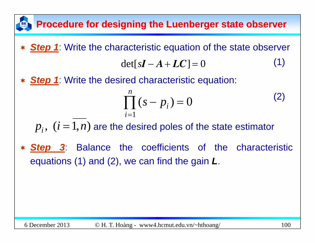
St 1 W it th h t i ti ti f th t t b Step 1: Write the characteristic equation of the state observer
0]det[ LCAIs (1)
Step 1: Write the desired characteristic equation:
0)( n
ips (2))(1i
ip
),1( , nipi are the desired poles of the state estimator
Step 3: Balance the coefficients of the characteristicequations (1) and (2), we can find the gain L.
6 December 2013 © H. T. Hoàng - www4.hcmut.edu.vn/~hthoang/ 100

Design of state estimators Design of state estimators –– ExampleExample
Problem: Given a system described by the state equation: Problem: Given a system described by the state equation:
)()()()()( tutt
CBAxx
)()( tty Cx
010 0 001C
100010
A
30
B 374 1
Assuming that the states of the system cannot be directly Assuming that the states of the system cannot be directlymeasured. Design the Luenberger state estimator so that thepoles of the state estimator lying at 20, 20 and 50.
6 December 2013 © H. T. Hoàng - www4.hcmut.edu.vn/~hthoang/ 101
p y g ,

Design of state estimators Design of state estimators –– Example (cont’)Example (cont’)
Solution The characteristic equation of the Luenberger state estimator:
0]det[ LCAIs
Solution
0]det[ LCAIs
0001100010
010001
d t1
ll
0001374
100100010det
3
2
lls
The desired characteristic equation:
(1)0)457()73()3( 321212
13 lllsllsls
The desired characteristic equation:
0)50()20( 2 ss23
6 December 2013 © H. T. Hoàng - www4.hcmut.edu.vn/~hthoang/ 102
(2)020000240090 23 sss
Design of state estimators Design of state estimators –– Example (cont’)Example (cont’)
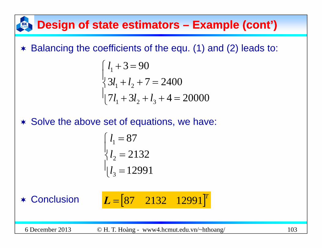
B l i th ffi i t f th (1) d (2) l d t Balancing the coefficients of the equ. (1) and (2) leads to:
9031l
20000437240073
321
21
lllll
Solve the above set of equations, we have:
87l
12991213287
2
1
lll
129913l
T12991213287L Conclusion
6 December 2013 © H. T. Hoàng - www4.hcmut.edu.vn/~hthoang/ 103
12991213287L Conclusion