fundamentals of probabilitybayanbox.ir/view/1975415597659025907/fundamentals-of... ·...
TRANSCRIPT

Instructor's Solutions Manual
Third Edition
F u n d a m e n t a l s o f
P r o b a b i l i t YWith Stochastic Processes
SAEED GHAHRAMANI
Western New England College
Upper Saddle River, New Jersey 07458


Contents
� 1 Axioms of Probability 1
1.2 Sample Space and Events 11.4 Basic Theorems 21.7 Random Selection of Points from Intervals 7
Review Problems 9
� 2 Combinatorial Methods 13
2.2 Counting Principle 132.3 Permutations 162.4 Combinations 182.5 Stirling’ Formula 31
Review Problems 31
� 3 Conditional Probability and Independence 35
3.1 Conditional Probability 353.2 Law of Multiplication 393.3 Law of Total Probability 413.4 Bayes’ Formula 463.5 Independence 483.6 Applications of Probability to Genetics 56
Review Problems 59
� 4 Distribution Functions andDiscrete Random Variables
63
4.2 Distribution Functions 634.3 Discrete Random Variables 664.4 Expectations of Discrete Random Variables 714.5 Variances and Moments of Discrete Random Variables 774.6 Standardized Random Variables 83
Review Problems 83

iv Contents
� 5 Special Discrete Distributions 87
5.1 Bernoulli and Binomial Random Variables 875.2 Poisson Random Variable 945.3 Other Discrete Random Variables 99
Review Problems 106
� 6 Continuous Random Variables 111
6.1 Probability Density Functions 1116.2 Density Function of a Function of a Random Variable 1136.3 Expectations and Variances 116
Review Problems 123
� 7 Special Continuous Distributions 126
7.1 Uniform Random Variable 1267.2 Normal Random Variable 1317.3 Exponential Random Variables 1397.4 Gamma Distribution 1447.5 Beta Distribution 1477.6 Survival Analysis and Hazard Function 152
Review Problems 153
� 8 Bivariate Distributions 157
8.1 Joint Distribution of Two Random Variables 1578.2 Independent Random Variables 1668.3 Conditional Distributions 1748.4 Transformations of Two Random Variables 183
Review Problems 191
� 9 Multivariate Distributions 200
9.1 Joint Distribution of n > 2 Random Variables 2009.2 Order Statistics 2109.3 Multinomial Distributions 215
Review Problems 218

Contents v
� 10 More Expectations and Variances 222
10.1 Expected Values of Sums of Random Variables 22210.2 Covariance 22710.3 Correlation 23710.4 Conditioning on Random Variables 23910.5 Bivariate Normal Distribution 251
Review Problems 254
� 11 Sums of Independent RandomVariables and Limit Theorems
261
11.1 Moment-Generating Functions 26111.2 Sums of Independent Random Variables 26911.3 Markov and Chebyshev Inequalities 27411.4 Laws of Large Numbers 27811.5 Central Limit Theorem 282
Review Problems 287
� 12 Stochastic Processes 291
12.2 More on Poisson Processes 29112.3 Markov Chains 29612.4 Continuous-Time Markov Chains 31512.5 Brownian Motion 326
Review Problems 331


Chapter 1
Axioms of Probability
1.2 SAMPLE SPACE AND EVENTS
1. For 1 ≤ i, j ≤ 3, by (i, j) we mean that Vann’s card number is i, and Paul’s card number isj . Clearly, A = {
(1, 2), (1, 3), (2, 3)}
and B = {(2, 1), (3, 1), (3, 2)
}.
(a) Since A ∩ B = ∅, the events A and B are mutually exclusive.
(b) None of (1, 1), (2, 2), (3, 3) belongs to A∪B. Hence A∪B not being the sample spaceshows that A and B are not complements of one another.
2. S = {RRR, RRB, RBR, RBB, BRR, BRB, BBR, BBB}.3. {x : 0 < x < 20}; {1, 2, 3, . . . , 19}.4. Denote the dictionaries by d1, d2; the third book by a. The answers are
{d1d2a, d1ad2, d2d1a, d2ad1, ad1d2, ad2d1} and {d1d2a, ad1d2}.5. EF : One 1 and one even.
EcF : One 1 and one odd.
EcF c: Both even or both belong to {3, 5}.6. S = {QQ, QN, QP, QD, DN, DP, NP, NN, PP }. (a) {QP }; (b) {DN, DP, NN}; (c) ∅.
7. S = {x : 7 ≤ x ≤ 9 1
6
};{x : 7 ≤ x ≤ 7 1
4
} ∪ {x : 7 34 ≤ x ≤ 8 1
4
} ∪ {x : 8 34 ≤ x ≤ 9 1
6
}.
8. E ∪ F ∪ G = G: If E or F occurs, then G occurs.
EFG = G: If G occurs, then E and F occur.
9. For 1 ≤ i ≤ 3, 1 ≤ j ≤ 3, by aibj we mean passenger a gets off at hotel i and passenger b
gets off at hotel j . The answers are {aibj : 1 ≤ i ≤ 3, 1 ≤ j ≤ 3} and {a1b1, a2b2, a3b3},respectively.
10. (a) (E ∪ F)(F ∪ G) = (F ∪ E)(F ∪ G) = F ∪ EG.

2 Chapter 1 Axioms of Probability
(b) Using part (a), we have
(E ∪ F)(Ec ∪ F)(E ∪ Fc) = (F ∪ EEc)(E ∪ Fc) = F(E ∪ Fc) = FE ∪ FFc = FE.
11. (a) ABcCc; (b) A ∪ B ∪ C; (c) AcBcCc; (d) ABCc ∪ ABcC ∪ AcBC;
(e) ABcCc ∪ AcBcC ∪ AcBCc; (f) (A − B) ∪ (B − A) = (A ∪ B) − AB.
12. If B = ∅, the relation is obvious. If the relation is true for every event A, then it is true for S,the sample space, as well. Thus
S = (B ∩ Sc) ∪ (Bc ∩ S) = ∅ ∪ Bc = Bc,
showing that B = ∅.
13. Parts (a) and (d) are obviously true; part (c) is true by DeMorgan’s law; part (b) is false: throwa four-sided die; let F = {1, 2, 3}, G = {2, 3, 4}, E = {1, 4}.
14. (a)⋃∞
n=1 An; (b)⋃37
n=1 An.
15. Straightforward.
16. Straightforward.
17. Straightforward.
18. Let a1, a2, and a3 be the first, the second, and the third volumes of the dictionary. Let a4, a5,a6, and a7 be the remaining books. Let A = {a1, a2, . . . , a7}; the answers are
S = {x1x2x3x4x5x6x7 : xi ∈ A, 1 ≤ i ≤ 7, and xi �= xj if i �= j
}and {
x1x2x3x4x5x6x7 ∈ S : xixi+1xi+2 = a1a2a3 for some i, 1 ≤ i ≤ 5},
respectively.
19.⋂∞
m=1
⋃∞n=m An.
20. Let B1 = A1, B2 = A2 − A1, B3 = A3 − (A1 ∪ A2), . . . , Bn = An −⋃n−1i=1 Ai , . . . .
1.4 BASIC THEOREMS
1. No; P(sum 11) = 2/36 while P(sum 12) = 1/36.
2. 0.33 + 0.07 = 0.40.

Section 1.4 Basic Theorems 3
3. Let E be the event that an earthquake will damage the structure next year. Let H be theevent that a hurricane will damage the structure next year. We are given that P(E) = 0.015,P(H) = 0.025, and P(EH) = 0.0073. Since
P(E ∪ H) = P(E) + P(H) − P(EH) = 0.015 + 0.025 − 0.0073 = 0.0327,
the probability that next year the structure will be damaged by an earthquake and/or a hurricaneis 0.0327. The probability that it is not damaged by any of the two natural disasters is 0.9673.
4. Let A be the event of a randomly selected driver having an accident during the next 12 months.Let B be the event that the person is male. By Theorem 1.7, the desired probability is
P(A) = P(AB) + P(ABc) = 0.12 + 0.06 = 0.18.
5. Let A be the event that a randomly selected investor invests in traditional annuities. Let B bethe event that he or she invests in the stock market. Then P(A) = 0.75, P(B) = 0.45, andP(A ∪ B) = 0.85. Since,
P(AB) = P(A) + P(B) − P(A ∪ B) = 0.75 + 0.45 − 0.85 = 0.35,
35% invest in both stock market and traditional annuities.
6. The probability that the first horse wins is 2/7. The probability that the second horse winsis 3/10. Since the events that the first horse wins and the second horse wins are mutuallyexclusive, the probability that either the first horse or the second horse will win is
2
7+ 3
10= 41
70.
7. In point of fact Rockford was right the first time. The reporter is assuming that both autopsiesare performed by a given doctor. The probability that both autopsies are performed by the samedoctor–whichever doctor it may be–is 1/2. Let AB represent the case in which Dr. A performsthe first autopsy and Dr. B performs the second autopsy, with similar representations for othercases. Then the sample space is S = {AA, AB, BA, BB}. The event that both autopsies areperformed by the same doctor is {AA, BB}. Clearly, the probability of this event is 2/4=1/2.
8. Let m be the probability that Marty will be hired. Then m + (m + 0.2) + m = 1 which givesm = 8/30; so the answer is 8/30 + 2/10 = 7/15.
9. Let s be the probability that the patient selected at random suffers from schizophrenia. Thens + s/3 + s/2 + s/10 = 1 which gives s = 15/29.
10. P(A ∪ B) ≤ 1 implies that P(A) + P(B) − P(AB) ≤ 1.
11. (a) 2/52 + 2/52 = 1/13; (b) 12/52 + 26/52 − 6/53 = 8/13; (c) 1 − (16/52) = 9/13.

4 Chapter 1 Axioms of Probability
12. (a) False; toss a die and let A = {1, 2}, B = {2, 3}, and C = {1, 3}.(b) False; toss a die and let A = {1, 2, 3, 4}, B = {1, 2, 3, 4, 5}, C = {1, 2, 3, 4, 5, 6}.
13. A simple Venn diagram shows that the answers are 65% and 10%, respectively.
14. Applying Theorem 1.6 twice, we have
P(A ∪ B ∪ C) = P(A ∪ B) + P(C) − P((A ∪ B)C
)= P(A) + P(B) − P(AB) + P(C) − P(AC ∪ BC)
= P(A) + P(B) − P(AB) + P(C) − P(AC) − P(BC) + P(ABC)
= P(A) + P(B) + P(C) − P(AB) − P(AC) − P(BC) + P(ABC).
15. Using Theorem 1.5, we have that the desired probability is
P(AB − ABC) + P(AC − ABC) + P(BC − ABC)
= P(AB) − P(ABC) + P(AC) − P(ABC) + P(BC) − P(ABC)
= P(AB) + P(AC) + P(BC) − 3P(ABC).
16. 7/11.
17.∑n
i=1 pij .
18. Let M and F denote the events that the randomly selected student earned an A on the midtermexam and an A on the final exam, respectively. Then
P(MF) = P(M) + P(F) − P(M ∪ F),
where P(M) = 17/33, P(F) = 14/33, and by DeMorgan’s law,
P(M ∪ F) = 1 − P(McF c) = 1 − 11
33= 22
33.
Therefore,
P(MF) = 17
33+ 14
33− 22
33= 3
11.
19. A Venn diagram shows that the answers are 1/8, 5/24, and 5/24, respectively.
20. The equation has real roots if and only if b2 ≥ 4c. From the 36 possible outcomes for (b, c),in the following 19 cases we have that b2 ≥ 4c: (2, 1), (3, 1), (3, 2), (4, 1), . . . , (4, 4), (5, 1),. . . , (5, 6), (6, 1), . . . , (6, 6). Therefore, the answer is 19/36.
21. The only prime divisors of 63 are 3 and 7. Thus the number selected is relatively prime to 63if and only if it is neither divisible by 3 nor by 7. Let A and B be the events that the outcome

Section 1.4 Basic Theorems 5
is divisible by 3 and 7, respectively. The desired quantity is
P(AcBc) = 1 − P(A ∪ B) = 1 − P(A) − P(B) + P(AB)
= 1 − 21
63− 9
63+ 3
63= 4
7.
22. Let T and F be the events that the number selected is divisible by 3 and 5, respectively.
(a) The desired quantity is the probability of the event T F c:
P(T F c) = P(T ) − P(T F) = 333
1000− 66
1000= 267
1000.
(b) The desired quantity is the probability of the event T cF c:
P(T cF c) = 1 − P(T ∪ F) = 1 − P(T ) − P(F) + P(T F)
= 1 − 333
1000− 200
1000+ 66
1000= 533
1000.
23. (Draw a Venn diagram.) From the data we have that 55% passed all three, 5% passed calculusand physics but not chemistry, and 20% passed calculus and chemistry but not physics. So atleast (55+5+20)% = 80% must have passed calculus. This number is greater than the given78% for all of the students who passed calculus. Therefore, the data is incorrect.
24. By symmetry the answer is 1/4.
25. Let A, B, and C be the events that the number selected is divisible by 4, 5, and 7, respectively.We are interested in P(ABcCc). Now ABcCc = A − A(B ∪ C) and A(B ∪ C) ⊆ A. So byTheorem 1.5,
P(ABcCc) = P(A) − P(A(B ∪ C)
) = P(A) − P(AB ∪ AC)
= P(A) − P(AB) − P(AC) + P(ABC)
= 250
1000− 50
1000− 35
1000+ 7
1000= 172
1000.
26. A Venn diagram shows that the answer is 0.36.
27. Let A be the event that the first number selected is greater than the second; let B be theevent that the second number selected is greater than the first; and let C be the event thatthe two numbers selected are equal. Then P(A) + P(B) + P(C) = 1, P(A) = P(B), andP(C) = 1/100. These give P(A) = 99/200.
28. Let B1 = A1, and for n ≥ 2, Bn = An − ⋃n−1i=1 Ai . Then {B1, B2, . . . } is a sequence of
mutually exclusive events and⋃∞
i=1 Ai = ⋃∞i=1 Bi. Hence

6 Chapter 1 Axioms of Probability
P( ∞⋃
n=1
An
)= P
( ∞⋃n=1
Bn
)=
∞∑n=1
P(Bn) ≤∞∑
n=1
P(An),
since Bn ⊆ An, n ≥ 1.
29. By Boole’s inequality (Exercise 28),
P( ∞⋂
n=1
An
)= 1 − P
( ∞⋃n=1
Acn
)≥ 1 −
∞∑n=1
P(Acn).
30. She is wrong! Consider the next 50 flights. For 1 ≤ i ≤ 50, let Ai be the event that the ithmission will be completed without mishap. Then
⋂50i=1 Ai is the event that all of the next 50
missions will be completed successfully. We will show that P(⋂50
i=1 Ai
)> 0. This proves
that Mia is wrong. Note that the probability of the simultaneous occurrence of any number ofAc
i ’s is nonzero. Furthermore, consider any set E consisting of n (n ≤ 50) of the Aci ’s. It is
reasonable to assume that the probability of the simultaneous occurrence of the events of E isstrictly less than the probability of the simultaneous occurrence of the events of any subset ofE. Using these facts, it is straightforward to conclude from the inclusion–exclusion principlethat,
P( 50⋃
i=1
Aci
)<
50∑i=1
P(Aci ) =
50∑i=1
1
50= 1.
Thus, by DeMorgan’s law,
P( 50⋂
i=1
Ai
)= 1 − P
( 50⋃i=1
Aci
)> 1 − 1 = 0.
31. Q satisfies Axioms 1 and 2, but not necessarily Axiom 3. So it is not, in general, a probabilityon S. Let S = {1, 2, 3, }. Let P
({1}) = P({2}) = P
({3}) = 1/3. Then Q({1}) = Q
({2}) =1/9, whereas Q
({1, 2}) = P({1, 2})2 = 4/9. Therefore,
Q({1, 2, }) �= Q
({1})+ Q({2}).
R is not a probability on S because it does not satisfy Axiom 2; that is, R(S) �= 1.
32. Let BRB mean that a blue hat is placed on the first player’s head, a red hat on the secondplayer’s head, and a blue hat on the third player’s head, with similar representations for othercases. The sample space is
S = {BBB, BRB, BBR, BRR, RRR, RRB, RBR, RBB}.This shows that the probability that two of the players will have hats of the same color andthe third player’s hat will be of the opposite color is 6/8 = 3/4. The following improvement,

Section 1.7 Random Selection of Points from Intervals 7
based on this observation, explained by Sara Robinson in Tuesday, April 10, 2001 issue ofthe New York Times, is due to Professor Elwyn Berlekamp of the University of California atBerkeley.
Three-fourths of the time, two of the players will have hats of the same color andthe third player’s hat will be the opposite color. The group can win every time thishappens by using the following strategy: Once the game starts, each player looksat the other two players’ hats. If the two hats are different colors, he [or she] passes.If they are the same color, the player guesses his [or her] own hat is the oppositecolor. This way, every time the hat colors are distributed two and one, one playerwill guess correctly and the others will pass, and the group will win the game. Whenall the hats are the same color, however, all three players will guess incorrectly andthe group will lose.
1.7 RANDOM SELECTION OF POINTS FROM INTERVALS
1.30 − 10
30 − 0= 2
3.
2.0.0635 − 0.04
0.12 − 0.04= 0.294.
3. (a) False; in the experiment of choosing a point at random from the interval (0, 1), letA = (0, 1) − {1/2}. A is not the sample space but P(A) = 1.(b) False; in the same experiment P
({1/2}) = 0 while { 12 } �= ∅.
4. P(A ∪ B) ≥ P(A) = 1, so P(A ∪ B) = 1. This gives
P(AB) = P(A) + P(B) − P(A ∪ B) = 1 + 1 − 1 = 1.
5. The answer is
P({1, 2, . . . , 1999}) =
1999∑i=1
P({i}) =
1999∑i=1
0 = 0.
6. For i = 0, 1, 2, . . . , 9, the probability that i appears as the first digit of the decimal represen-
tation of the selected point is the probability that the point falls into the interval[ i
10,i + 1
10
).
Therefore, it equalsi + 1
10− i
101 − 0
= 1
10.
This shows that all numerals are equally likely to appear as the first digit of the decimalrepresentation of the selected point.

8 Chapter 1 Axioms of Probability
7. No, it is not. Let S = {w1, w2, . . . }. Suppose that for some p > 0, P({wi}
) = p, i = 1, 2,. . . . Then, by Axioms 2 and 3,
∑∞i=1 p = 1. This is impossible.
8. Use induction. For n = 1, the theorem is trivial. Exercise 4 proves the theorem for n = 2.Suppose that the theorem is true for n. We show it for n + 1,
P(A1A2 · · · AnAn+1) = P(A1A2 · · · An) + P(An+1) − P(A1A2 · · · An ∪ An+1)
= 1 + 1 − 1 = 1,
where P(A1A2 · · · An) = 1 is true by the induction hypothesis, and
P(A1A2 · · · An ∪ An+1) ≥ P(An+1) = 1,
implies that P(A1A2 · · · An ∪ An+1) = 1.
9. (a) Clearly,1
2∈
∞⋂n=1
(1
2− 1
2n,
1
2+ 1
2n
). If x ∈
∞⋂n=1
(1
2− 1
2n,
1
2+ 1
2n
), then, for all n ≥ 1,
1
2− 1
2n< x <
1
2+ 1
2n.
Letting n → ∞, we obtain 1/2 ≤ x ≤ 1/2; thus x = 1/2.
(b) Let An be the event that the point selected at random is in(1
2− 1
2n,
1
2+ 1
2n
); then
A1 ⊇ A2 ⊇ A3 ⊇ · · · ⊇ An ⊇ An+1 ⊇ · · · .
Since P(An) = 1
n, by the continuity property of the probability function,
P({1/2}) = lim
n→∞ P(An) = 0.
10. The set of rational numbers is countable. Let Q = {r1, r2, r3, . . . } be the set of rationalnumbers in (0, 1). Then
P(Q) = P({r1, r2, r3, . . . }
) =∞∑i=1
P({ri}
) = 0.
Let I be the set of irrational numbers in (0, 1); then
P(I) = P(Qc) = 1 − P(Q) = 1.
11. For i = 0, 1, 2, . . . , 9, the probability that i appears as the nth digit of the decimal represen-tation of the selected point is the probability that the point falls into the following subset of(0, 1):
10n−1−1⋃m=0
[10m + i
10n,
10m + i + 1
10n
).

Chapter 1 Review Problems 9
Since the intervals in this union are mutually exclusive, the probability that the point falls intothis subset is
10n−1−1∑m=0
10m + i + 1
10n− 10m + i
10n
1 − 0= 10n−1 · 1
10n= 1
10.
This shows that all numerals are equally likely to appear as the nth digit of the decimalrepresentation of the selected point.
12. P(Bm) ≤ ∑∞n=m P (An). Since
∑∞n=1 P(An) converges,
limm→∞ P(Bm) ≤ lim
m→∞
∞∑n=m
P (An) = 0.
This gives limm→∞ P(Bm) = 0. Therefore,
B1 ⊇ B2 ⊇ B3 ⊇ · · · ⊇ Bm ⊇ Bm+1 ⊇ · · ·implies that
P( ∞⋂
m=1
∞⋃n=m
An
)= P
( ∞⋂m=1
Bm
)= lim
m→∞ P(Bm) = 0.
13. In the experiment of choosing a random point from (0, 1), let Et = (0, 1)−{t}, for 0 < t < 1.Then P(Et) = 1 for all t , while
P( ⋂
t∈(0,1)
Et
)= P(∅) = 0.
14. Clearly rn ∈ (αn, βn). By the geometric series theorem,
∞∑n=1
(βn − αn) =∞∑
n=1
ε
2n+1= ε
1
4
1 − 1
2
= ε
2< ε.
REVIEW PROBLEMS FOR CHAPTER 1
1.3.25 − 2
4.3 − 2= 0.54.
2. We have that
S ={(∅, {1}), (∅, {2}), (∅, {1, 2}), ({1}, {2}), ({1}, {1, 2}), ({2}, {1, 2})}.

10 Chapter 1 Axioms of Probability
The desired events are
(a){(∅, {1}), (∅, {2}), (∅, {1, 2}), ({1}, {2})}; (b)
{(∅, {1, 2}), ({1}, {2})};(c)
{(∅, {1}), (∅, {2}), (∅, {1, 2}), ({1}, {1, 2}), ({2}, {1, 2})}.3. Since A ⊆ B, we have that Bc ⊆ Ac. This implies that (a) is false but (b) is true.
4. In the experiment of tossing a die let A = {1, 3, 5} and B = {5}; then both (a) and (b) arefalse.
5. We may define a sample space S as follows.
S = {x1x2 · · · xn : n ≥ 1, xi ∈ {H,T}; xi �= xi+1, 1 ≤ i ≤ n − 2; xn−1 = xn
}.
6. A venn diagram shows that 18 are neither male nor for surgery.
7. We have that ABC ⊆ BC, so P(ABC) ≤ P(BC) and hence P(BC) − P(ABC) ≥ 0. Thisand the following give the result.
P(A ∪ B ∪ C) = P(A) + P(B) + P(C) − [P(AB) + P(AC) + P(BC) − P(ABC)
]≤ P(A) + P(B) + P(C).
8. If P(AB) = P(AC) = P(BC) = 0, then P(ABC) = 0 since ABC ⊆ AB. These imply that
P(A ∪ B ∪ C) = P(A) + P(B) + P(C) − P(AB) − P(AC) − P(BC) + P(ABC)
= P(A) + P(B) + P(C).
Now suppose thatP(A ∪ B ∪ C) = P(A) + P(B) + P(C).
This relation implies that
P(AB) + P(BC) + [P(AC) − P(ABC)
] = 0. (1)
Since P(AC) − P(ABC) ≥ 0 we have that the sum of three nonnegative quantities is 0; soeach of them is 0. That is,
P(AB) = 0, P (BC) = 0, P (AC) = P(ABC). (2)
Now rewriting (1) as
P(AB) + P(AC) + [P(BC) − P(ABC)
] = 0,
the same argument implies that
P(AB) = 0, P (AC) = 0, P (BC) = P(ABC). (3)
Comparing (2) and (3) we have
P(AB) = P(AC) = P(BC) = 0.

Chapter 1 Review Problems 11
9. Let W be the event that a randomly selected person from this community drinks or serveswhite wine. Let R be the event that she or he drinks or serves red wine. We are given thatP(W) = 0.40, P(R) = 0.50, and P(W ∪ R) = 0.70. Since
P(WR) = P(W) + P(R) − P(W ∪ R) = 0.40 + 0.50 − 0.70 = 0.20,
20% percent drink or serve both red and white wine.
10. No, it is not right. The probability that the second student chooses the tire the first studentchose is 1/4.
11. By De Morgan’s second law,
P(AcBc) = 1 − P((AcBc)c
) = 1 − P(A ∪ B) = 1 − P(A) − P(B) + P(AB).
12. By Theorem 1.5 and the fact that A − B and B − A are mutually exclusive,
P((A − B) ∪ (B − A)
) = P(A − B) + P(B − A) = P(A − AB) + P(B − AB)
= P(A) − P(AB) + P(B) − P(AB) = P(A) + P(B) − 2P(AB).
13. Denote a box of books by ai , if it is received from publisher i, i = 1, 2, 3. The sample spaceis
S = {x1x2x3x4x5x6 : two of the xi’s are a1, two of them are a2, and the remaining two are a3
}.
The desired event is E = {x1x2x3x4x5x6 ∈ S : x5 = x6
}.
14. Let E, F , G, and H be the events that the next baby born in this town has blood type O, A, B,and AB, respectively. Then
P(E) = P(F), P (G) = 1
10P(F), P (G) = 2P(H).
These implyP(E) = P(F) = 20P(H).
Therefore, fromP(E) + P(F) + P(G) + P(H) = 1,
we get20P(H) + 20P(H) + 2P(H) + P(H) = 1,
which gives P(H) = 1/43.
15. Let F , S, and N be the events that the number selected is divisible by 4, 7, and 9, respectively.We are interested in P(F cScNc) which is equal to 1 − P(F ∪ S ∪ N) by DeMorgan’s law.

12 Chapter 1 Axioms of Probability
Now
P(F ∪ S ∪ N) = P(F) + P(S) + P(N) − P(FS) − P(FN) − P(SN) + P(FSN)
= 250
1000+ 142
1000+ 111
1000− 35
1000− 27
1000− 15
1000+ 3
1000= 0.429.
So the desired probability is 0.571.
16. The number is relatively prime to 150 if is not divisible by 2, 3, or 5. Let A, B, and C be theevents that the number selected is divisible by 2, 3, and 5, respectively. We are interested inP(AcBcCc) = 1 − P(A ∪ B ∪ C). Now
P(A ∪ B ∪ C) = P(A) + P(B) + P(C) − P(AB) − P(AC) − P(BC) + P(ABC)
= 75
150+ 50
150+ 30
150− 25
150− 15
150− 10
150+ 5
150= 11
15.
Therefore, the answer is 1 − 11
15= 4
15.
17. (a) Uci Dc
i ; (b) U1U2 · · · Un; (c) (Uc1 Dc
1) ∪ (Uc2 Dc
2) ∪ · · · ∪ (UcnDc
n);(d) (U1D2U
c3 Dc
3) ∪ (U1Uc2 Dc
2D3) ∪ (D1U2Uc3 Dc
3) ∪ (D1Uc2 Dc
2U3)
∪(Dc1U
c1 D2U3) ∪ (Dc
1Uc1 U2D2) ∪ (Dc
1Uc1 Dc
2Uc2 Dc
3Uc3 );
(e) Dc1D
c2 · · · Dc
n.
18.199 − 96
199 − 0= 103
199.
19. We must have b2 < 4ac. There are 6 × 6 × 6 = 216 possible outcomes for a, b, and c. Forcases in which a < c, a > c, and a = c, it can be checked that there are 73, 73, and 27 casesin which b2 < 4ac, respectively. Therefore, the desired probability is
73 + 73 + 27
216= 173
216.
Chapter 2
Combinatorial Methods
2.2 COUNTING PRINCIPLES
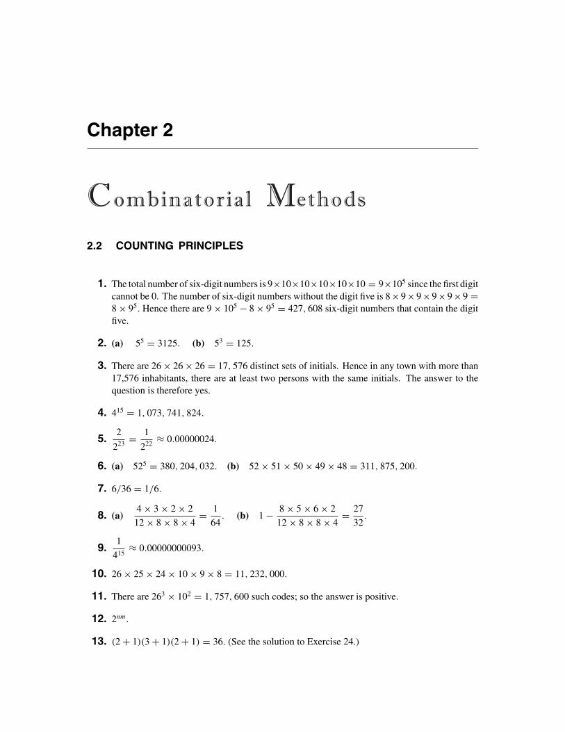
1. The total number of six-digit numbers is 9×10×10×10×10×10 = 9×10⁵ since the first digitcannot be 0. The number of six-digit numbers without the digit five is 8×9×9×9×9×9 =8 × 95. Hence there are 9 × 10⁵ − 8 × 95 = 427, 608 six-digit numbers that contain the digitfive.
2. (a) 55 = 3125. (b) 53 = 125.
3. There are 26 × 26 × 26 = 17, 576 distinct sets of initials. Hence in any town with more than17,576 inhabitants, there are at least two persons with the same initials. The answer to thequestion is therefore yes.
4. 415 = 1, 073, 741, 824.
5.2
223 = 1
222 ≈ 0.00000024.
6. (a) 525 = 380, 204, 032. (b) 52 × 51 × 50 × 49 × 48 = 311, 875, 200.
7. 6/36 = 1/6.
8. (a)4 × 3 × 2 × 2
12 × 8 × 8 × 4= 1
64. (b) 1 − 8 × 5 × 6 × 2
12 × 8 × 8 × 4= 27
32.
9.1
415≈ 0.00000000093.
10. 26 × 25 × 24 × 10 × 9 × 8 = 11, 232, 000.
11. There are 263 × 102 = 1, 757, 600 such codes; so the answer is positive.
12. 2nm.
13. (2 + 1)(3 + 1)(2 + 1) = 36. (See the solution to Exercise 24.)

14 Chapter 2 Combinatorial Methods
14. There are (26 − 1)23 = 504 possible sandwiches. So the claim is true.
15. (a) 54 = 625. (b) 54 − 5 × 4 × 3 × 2 = 505.
16. 212 = 4096.
17. 1 − 48 × 48 × 48 × 48
52 × 52 × 52 × 52= 0.274.
18. 10 × 9 × 8 × 7 = 5040. (a) 9 × 9 × 8 × 7 = 4536; (b) 5040 − 1 × 1 × 8 × 7 = 4984.
19. 1 − (N − 1)n
Nn.
20. By Example 2.6, the probability is 0.507 that among Jenny and the next 22 people she meetsrandomly there are two with the same birthday. However, it is quite possible that one of thesetwo persons is not Jenny. Let n be the minimum number of people Jenny must meet so thatthe chances are better than even that someone shares her birthday. To find n, let A denote theevent that among the next n people Jenny meets randomly someone’s birthday is the same asJenny’s. We have
P(A) = 1 − P(Ac) = 1 − 364n
365n.
To have P(A) > 1/2, we must find the smallest n for which
1 − 364n
365n>
1
2,
or364n
365n<
1
2.
This gives
n >
log1
2
log364
365
= 252.652.
Therefore, for the desired probability to be greater than 0.5, n must be 253. To some this mightseem counterintuitive.
21. Draw a tree diagram for the situation in which the salesperson goes from I to B first. Inthis situation, you will find that in 7 out of 23 cases, she will end up staying at island I . Bysymmetry, if she goes from I to H , D, or F first, in each of these situations in 7 out of 23cases she will end up staying at island I . So there are 4 × 23 = 92 cases altogether and in4×7 = 28 of them the salesperson will end up staying at island I . Since 28/92 = 0.3043, theanswer is 30.43%. Note that the probability that the salesperson will end up staying at islandI is not 0.3043 because not all of the cases are equiprobable.

Section 2.2 Counting Principle 15
22. He is at 0 first, next he goes to 1 or −1. If at 1, then he goes to 0 or 2. If at −1, then he goesto 0 or −2, and so on. Draw a tree diagram. You will find that after walking 4 blocks, he is atone of the points 4, 2, 0, −2, or −4. There are 16 possible cases altogether. Of these 6 end upat 0, none at 1, and none at −1. Therefore, the answer to (a) is 6/16 and the answer to (b) is 0.
23. We can think of a number less than 1,000,000 as a six-digit number by allowing it to start with0 or 0’s. With this convention, it should be clear that there are 96 such numbers without thedigit five. Hence the desired probability is 1 − (96/106) = 0.469.
24. Divisors of N are of the form pe11 p
e22 · · · pek
k , where ei = 0, 1, 2, . . . , ni , 1 ≤ i ≤ k. Therefore,the answer is (n1 + 1)(n2 + 1) · · · (nk + 1).
25. There are 64 possibilities altogether. In 54 of these possibilities there is no 3. In 53 of thesepossibilities only the first die lands 3. In 53 of these possibilities only the second die lands 3,and so on. Therefore, the answer is
54 + 4 × 53
64= 0.868.
26. Any subset of the set {salami, turkey, bologna, corned beef, ham, Swiss cheese, Americancheese} except the empty set can form a reasonable sandwich. There are 27 − 1 possibilities.To every sandwich a subset of the set {lettuce, tomato, mayonnaise} can also be added. Sincethere are 3 possibilities for bread, the final answer is (27 − 1) × 23 × 3 = 3048 and theadvertisement is true.
27.11 × 10 × 9 × 8 × 7 × 6 × 5 × 4
118= 0.031.
28. For i = 1, 2, 3, let Ai be the event that no one departs at stop i. The desired quantity isP(Ac
1Ac2A
c3) = 1 − P(A1 ∪ A2 ∪ A3). Now
P(A1 ∪ A2 ∪ A3) = P(A1) + P(A2) + P(A3)
− P(A1A2) − P(A1A3) − P(A2A3) + P(A1A2A3)
= 26
36+ 26
36+ 26
36− 1
36− 1
36− 1
36+ 0 = 7
27.
Therefore, the desired probability is 1 − (7/27) = 20/27.
29. For 0 ≤ i ≤ 9, the sum of the first two digits is i in (i + 1) ways. Therefore, there are (i + 1)2
numbers in the given set with the sum of the first two digits equal to the sum of the last twodigits and equal to i. For i = 10, there are 92 numbers in the given set with the sum of the firsttwo digits equal to the sum of the last two digits and equal to 10. For i = 11, the correspondingnumbers are 82 and so on. Therefore, there are altogether
12 + 22 + · · · + 102 + 92 + 82 + · · · + 12 = 670

16 Chapter 2 Combinatorial Methods
numbers with the desired probability and hence the answer is 670/104 = 0.067.
30. Let A be the event that the number selected contains at least one 0. Let B be the event that itcontains at least one 1 and C be the event that it contains at least one 2. The desired quantityis P(ABC) = 1 − P(Ac ∪ Bc ∪ Cc), where
P(Ac ∪ Bc ∪ Cc) = P(Ac) + P(Bc) + P(Cc)
− P(AcBc) − P(AcCc) − P(BcCc) + P(AcBcCc)
= 9r
9 × 10r−1+ 8 × 9r−1
9 × 10r−1+ 8 × 9r−1
9 × 10r−1− 8r
9 × 10r−1− 8r
9 × 10r−1
− 7 × 8r−1
9 × 10r−1+ 7 r
9 × 10r−1.
2.3 PERMUTATIONS
1. The answer is1
4! = 1
24≈ 0.0417.
2. 3! = 6.
3.8!
3! 5! = 56.
4. The probability that John will arrive right after Jim is 7!/8! (consider Jim and John as onearrival). Therefore, the answer is 1 − (7!/8!) = 0.875.
Another Solution: If Jim is the last person, John will not arrive after Jim. Therefore, theremaining seven can arrive in 7! ways. If Jim is not the last person, the total number ofpossibilities in which John will not arrive right after Jim is 7 × 6 × 6!. So the answer is
7! + 7 × 6 × 6!8! = 0.875.
5. (a) 312 = 531, 441. (b)12!6! 6! = 924. (c)
12!3! 4! 5! = 27, 720.
6. 6P2 = 30.
7.20!
4! 3! 5! 8! = 3, 491, 888, 400.
8.(5 × 4 × 7) × (4 × 3 × 6) × (3 × 2 × 5)
3! = 50, 400.

Section 2.3 Permutations 17
9. There are 8! schedule possibilities. By symmetry, in 8!/2 of them Dr. Richman’s lectureprecedes Dr. Chollet’s and in 8!/2 ways Dr. Richman’s lecture precedes Dr. Chollet’s. So theanswer is 8!/2 = 20, 160.
10.11!
3! 2! 3! 3! = 92, 400.
11. 1 − (6!/66) = 0.985.
12. (a)11!
4! 4! 2! = 34, 650.
(b) Treating all P ’s as one entity, the answer is10!4! 4! = 6300.
(c) Treating all I ’s as one entity, the answer is8!
4! 2! = 840.
(d) Treating all P ’s as one entity, and all I ’s as another entity, the answer is7!4! = 210.
(e) By (a) and (c), The answer is 840/34650 = 0.024.
13.( 8!
2! 3! 3!)/
68 = 0.000333.
14.( 9!
3! 3! 3!)/
529 = 6.043 × 10⁻¹³.
15.m!
(n + m)! .
16. Each girl and each boy has the same chance of occupying the 13th chair. So the answer is
12/20 = 0.6. This can also be seen from12 × 19!
20! = 12
20= 0.6.
17.12!1212
= 0.000054.
18. Look at the five math books as one entity. The answer is5! × 18!
22! = 0.00068.
19. 1 − 9P7
97= 0.962.
20.2 × 5! × 5!
10! = 0.0079.
21. n!/nn.

18 Chapter 2 Combinatorial Methods
22. 1 − (6!/66) = 0.985.
23. Suppose that A and B are not on speaking terms. 134P4 committees can be formed in whichneither A serves nor B; 4×134 P3 committees can be formed in which A serves and B does not.The same numbers of committees can be formed in which B serves and A does not. Therefore,the answer is 134P4 + 2(4 ×134 P3) = 326, 998, 056.
24. (a) mn. (b) mPn. (c) n!.
25.(
3 · 8!2! 3! 2! 1!
)/68 = 0.003.
26. (a)20!
39 × 37 × 35 × · · · × 5 × 3 × 1= 7.61 × 10⁻⁶.
(b)1
39 × 37 × 35 × · · · × 5 × 3 × 1= 3.13 × 10⁻²⁴.
27. Thirty people can sit in 30! ways at a round table. But for each way, if they rotate 30 times(everybody move one chair to the left at a time) no new situations will be created. Thus in30!/30 = 29! ways 15 married couples can sit at a round table. Think of each married coupleas one entity and note that in 15!/15 = 14! ways 15 such entities can sit at a round table. Wehave that the 15 couples can sit at a round table in (2!)15 · 14! different ways because if thecouples of each entity change positions between themselves, a new situation will be created.So the desired probability is
14!(2!)15
29! = 3.23 × 10⁻¹⁶.
The answer to the second part is
24!(2!)5
29! = 2.25 × 10⁻⁶.
28. In 13! ways the balls can be drawn one after another. The number of those in which the firstwhite appears in the second or in the fourth or in the sixth or in the eighth draw is calculatedas follows. (These are Jack’s turns.)
8 × 5 × 11! + 8 × 7 × 6 × 5 × 9! + 8 × 7 × 6 × 5 × 4 × 5 × 7!+ 8 × 7 × 6 × 5 × 4 × 3 × 2 × 5 × 5! = 2, 399, 846, 400.
Therefore, the answer is 2, 399, 846, 400/13! = 0.385.

Section 2.4 Combinations 19
2.4 COMBINATIONS
1.(
20
6
)= 38, 760.
2.100∑i=51
(100
i
)= 583, 379, 627, 841, 332, 604, 080, 945, 354, 060 ≈ 5.8 × 1029.
3.(
20
6
)(25
6
)= 6, 864, 396, 000.
4.
(12
3
)(40
2
)(
52
5
) = 0.066.
5.(
N − 1
n − 1
)/(N
n
)= n
N.
6.(
5
3
)(2
2
)= 10.
7.(
8
3
)(5
2
)(3
3
)= 560.
8.(
18
6
)+(
18
4
)= 21, 624.
9.(
10
5
)/(12
7
)= 0.318.
10. The coefficient of 23x9 in the expansion of (2 + x)12 is
(12
9
). Therefore, the coefficient of x9
is 23
(12
9
)= 1760.
11. The coefficient of (2x)3(−4y)4 in the expansion of (2x − 4y)7 is
(7
4
). Thus the coefficient
of x3y2 in this expansion is 23(−4)4
(7
4
)= 71, 680.
12.(
9
3
)[(6
4
)+ 2
(6
3
)]= 4620.

20 Chapter 2 Combinatorial Methods
13. (a)(
10
5
)/210 = 0.246; (b)
10∑i=5
(10
i
)/210 = 0.623.
14. If their minimum is larger than 5, they are all from the set {6, 7, 8, . . . , 20}. Hence the answer
is
(15
5
)/(20
5
)= 0.194.
15. (a)
(6
2
)(28
4
)(
34
6
) = 0.228; (b)
(6
6
)+(
6
6
)+(
10
6
)+(
12
6
)(
34
6
) = 0.00084.
16.
(50
5
)(150
45
)(
200
50
) = 0.00206.
17.n∑
i=0
2i
(n
i
)=
n∑i=0
(n
i
)2i1n−i = (2 + 1)n = 3n.
n∑i=0
xi
(n
i
)=
n∑i=0
(n
i
)xi1n−i = (x + 1)n.
18.[(6
2
)54]/
66 = 0.201.
19. 212/(24
12
)= 0.00151.
20. Royal Flush:4(
52
5
) = 0.0000015.
Straight flush:36(52
5
) = 0.000014.
Four of a kind:13 × 12
(4
1
)(
52
5
) = 0.00024.

Section 2.4 Combinations 21
Full house:13
(4
3
)· 12
(4
2
)(
52
5
) = 0.0014.
Flush:4
(13
5
)− 40(
52
5
) = 0.002.
Straight:10(4)5 − 40(
52
5
) = 0.0039.
Three of a kind:13
(4
3
)·(
12
2
)42(
52
5
) = 0.021.
Two pairs:
(13
2
)(4
2
)(4
2
)· 11
(4
1
)(
52
5
) = 0.048.
One pair:13
(4
2
)·(
12
3
)43(
52
5
) = 0.42.
None of the above: 1− the sum of all of the above cases = 0.5034445.
21. The desired probability is
(12
6
)(12
6
)(
24
12
) = 0.3157.
22. The answer is the solution of the equation
(x
3
)= 20. This equation is equivalent to
x(x − 1)(x − 2) = 120 and its solution is x = 6.

22 Chapter 2 Combinatorial Methods
23. There are 9×103 = 9000 four-digit numbers. From every 4-combination of the set {0, 1, . . . , 9},exactly one four-digit number can be constructed in which its ones place is less than its tensplace, its tens place is less than its hundreds place, and its hundreds place is less than its
thousands place. Therefore, the number of such four-digit numbers is
(10
4
)= 210. Hence
the desired probability is 0.023333.
24.
(x + y + z)2 =∑
n1+n2+n3=2
n!n1! n2! n3! xn1yn2zn3
= 2!2! 0! 0! x2y0z0 + 2!
0! 2! 0! x0y2z0 + 2!0! 0! 2! x0y0z2
+ 2!1! 1! 0! x1y1z0 + 2!
1! 0! 1! x1y0z1 + 2!0! 1! 1! x0y1z1
= x2 + y2 + z2 + 2xy + 2xz + 2yz.
25. The coefficient of (2x)2(−y)3(3z)2 in the expansion of (2x − y + 3z)7 is7!
2! 3! 2! . Thus the
coefficient of x2y3z2 in this expansion is 22(−1)3(3)2 7!2! 3! 2! = −7560.
26. The coefficient of (2x)3(−y)7(3)3 in the expansion of (2x − y + 3)13 is13!
3! 7! 3! . Therefore,
the coefficient of x3y7 in this expansion is 23(−1)7(3)3 13!3! 7! 3! = −7, 413, 120.
27. In52!
13! 13! 13! 13! = 52!(13!)4
ways 52 cards can be dealt among four people. Hence the sample
space contains 52!/(13!)4 points. Now in 4! ways the four different suits can be distributedamong the players; thus the desired probability is 4!/[52!/(13!)4] ≈ 4.47 × 10⁻²⁸.
28. The theorem is valid for k = 2; it is the binomial expansion. Suppose that it is true for allintegers ≤ k − 1. We show it for k. By the binomial expansion,
(x1 + x2 + · · · + xk)n =
n∑n1=0
(n
n1
)x
n11 (x2 + · · · + xk)
n−n1
=n∑
n1=0
(n
n1
)x
n11
∑n2+n3+···+nk=n−n1
(n − n1)!n2! n3! · · · nk! x
n22 x
n33 · · · xnk
k
=∑
n1+n2+···+nk=n
(n
n1
)(n − n1)!
n2! n3! · · · nk! xn11 x
n22 · · · xnk
k

Section 2.4 Combinations 23
=∑
n1+n2+···+nk=n
n!n1! n2! · · · nk! x
n11 x
n22 · · · xnk
k .
29. We must have 8 steps. Since the distance from M to L is ten 5-centimeter intervals and thefirst step is made at M, there are 9 spots left at which the remaining 7 steps can be made. So
the answer is
(9
7
)= 36.
30. (a)
(2
1
)(98
49
)+(
98
48
)(
100
50
) = 0.753; (b) 250/(100
50
)= 1.16 × 10⁻¹⁴.
31. (a) It must be clear that
n1 =(
n
2
)n2 =
(n1
2
)+ nn1
n3 =(
n2
2
)+ n2(n + n1)
n4 =(
n3
2
)+ n3(n + n1 + n2)
...
nk =(
nk−1
2
)+ nk−1(n + n1 + · · · + nk−1).
(b) For n = 25, 000, successive calculations of nk’s yield,
n1 = 312, 487, 500,
n2 = 48, 832, 030, 859, 381, 250,
n3 = 1, 192, 283, 634, 186, 401, 370, 231, 933, 886, 715, 625,
n4 = 710, 770, 132, 174, 366, 339, 321, 713, 883, 042, 336, 781, 236,
550, 151, 462, 446, 793, 456, 831, 056, 250.
For n = 25, 000, the total number of all possible hybrids in the first four generations,n1 +n2 +n3 +n4, is 710,770,132,174,366,339,321,713,883,042,337,973,520,184,337,863,865,857,421,889,665,625. This number is approximately 710 × 1063.
32. For n = 1, we have the trivial identity
x + y =(
1
0
)x0y1−0 +
(1
1
)x1y1−1.
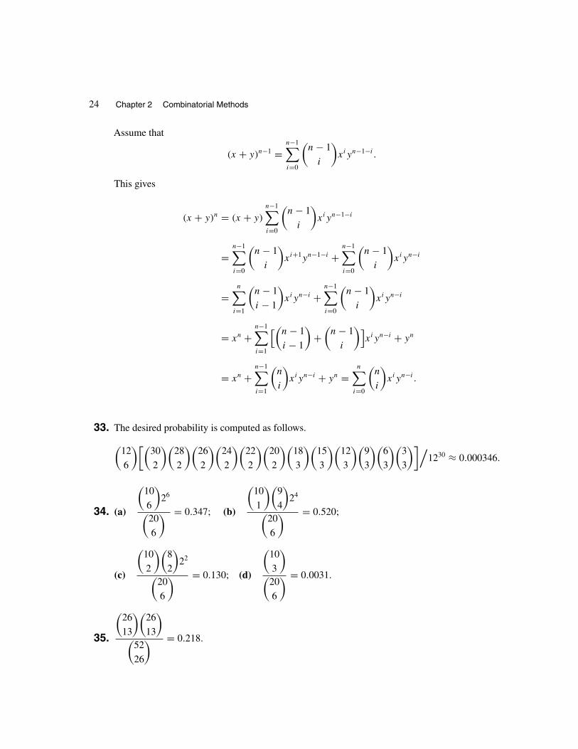
24 Chapter 2 Combinatorial Methods
Assume that
(x + y)n−1 =n−1∑i=0
(n − 1
i
)xiyn−1−i .
This gives
(x + y)n = (x + y)
n−1∑i=0
(n − 1
i
)xiyn−1−i
=n−1∑i=0
(n − 1
i
)xi+1yn−1−i +
n−1∑i=0
(n − 1
i
)xiyn−i
=n∑
i=1
(n − 1
i − 1
)xiyn−i +
n−1∑i=0
(n − 1
i
)xiyn−i
= xn +n−1∑i=1
[(n − 1
i − 1
)+(
n − 1
i
)]xiyn−i + yn
= xn +n−1∑i=1
(n
i
)xiyn−i + yn =
n∑i=0
(n
i
)xiyn−i .
33. The desired probability is computed as follows.(12
6
)[(30
2
)(28
2
)(26
2
)(24
2
)(22
2
)(20
2
)(18
3
)(15
3
)(12
3
)(9
3
)(6
3
)(3
3
)]/1230 ≈ 0.000346.
34. (a)
(10
6
)26(
20
6
) = 0.347; (b)
(10
1
)(9
4
)24(
20
6
) = 0.520;
(c)
(10
2
)(8
2
)22(
20
6
) = 0.130; (d)
(10
3
)(
20
6
) = 0.0031.
35.
(26
13
)(26
13
)(
52
26
) = 0.218.

Section 2.4 Combinations 25
36. Let a 6-element combination of a set of integers be denoted by {a1, a2, . . . , a6}, where a1 <
a2 < · · · < a6. It can be easily verified that the function h : B → A defined by
h({a1, a2, . . . , a6}
) = {a1, a2 + 1, . . . , a6 + 5}is one-to-one and onto. Therefore, there is a one-to-one correspondence between B and
A . This shows that the number of elements in A is
(44
6
). Thus the probability that no
consecutive integers are selected among the winning numbers is
(44
6
)/(49
6
)≈ 0.505. This
implies that the probability of at least two consecutive integers among the winning numbersis approximately 1 − 0.505 = 0.495. Given that there are 47 integers between 1 and 49, thishigh probability might be counter-intuitive. Even without knowledge of expected value, akeen student might observe that, on the average, there should be (49 − 1)/7 = 6.86 numbersbetween each ai and ai+1, 1 ≤ i ≤ 5. Thus he or she might erroneously think that it is unlikelyto obtain consecutive integers frequently.
37. (a) Let Ei be the event that car i remains unoccupied. The desired probability is
P(Ec1E
c2 · · · Ec
n) = 1 − P(E1 ∪ E2 ∪ · · · ∪ En).
Clearly,
P(Ei) = (n − 1)m
nm, 1 ≤ i ≤ n;
P(EiEj ) = (n − 2)m
nm, 1 ≤ i, j ≤ n, i �= j ;
P(EiEjEk) = (n − 3)m
nm, 1 ≤ i, j, k ≤ n, i �= j �= k;
and so on. Therefore, by the inclusion-exclusion principle,
P(E1 ∪ E2 ∪ · · · ∪ En) =n∑
i=1
(−1)i−1
(n
i
)(n − i)m
nm.
So
P(Ec1E
c2 · · · Ec
n) = 1 −n∑
i=1
(−1)i−1
(n
i
)(n − i)m
nm=
n∑i=0
(−1)i
(n
i
)(n − i)m
nm
= 1
nm
n∑i=0
(−1)i
(n
i
)(n − i)m.
(b) Let F be the event that cars 1, 2, . . . , n − r are all occupied and the remaining cars are
unoccupied. The desired probability is
(n
r
)P(F). Now by part (a), the number of ways m

26 Chapter 2 Combinatorial Methods
passengers can be distributed among n − r cars, no car remaining unoccupied is
n−r∑i=0
(−1)i
(n − r
i
)(n − r − i)m.
So
P(F) = 1
nm
n−r∑i=0
(−1)i
(n − r
i
)(n − r − i)m
and hence the desired probability is
1
nm
(n
r
) n−r∑i=0
(−1)i
(n − r
i
)(n − r − i)m.
38. Let the n indistinguishable balls be represented by n identical oranges and the n distinguishablecells be represented by n persons. We should count the number of different ways that the n
oranges can be divided among the n persons, and the number of different ways in which exactlyone person does not get an orange. The answer to the latter part is n(n − 1) since in this caseone person does not get an orange, one person gets exactly two oranges, and the remainingpersons each get exactly one orange. There are n choices for the person who does not getan orange and n − 1 choices for the person who gets exactly two oranges; n(n − 1) choicesaltogether. To count the number of different ways that the n oranges can be divided among then persons, add n − 1 identical apples to the oranges and note that by Theorem 2.4, the total
number of permutations of these n − 1 apples and n oranges is(2n − 1)!n! (n − 1)! . (We can arrange
n − 1 identical apples and n identical oranges in a row in (2n − 1)!/[n! (n − 1)!] ways.) Now
each one of these(2n − 1)!n! (n − 1)! =
(2n − 1
n
)permutations corresponds to a way of dividing the
n oranges among the n persons and vice versa. Give all of the oranges preceding the first appleto the first person, the oranges between the first and the second apples to the second person,the oranges between the second and the third apples to the third person and so on. Therefore,if, for example, an apple appears in the beginning of the permutation, the first person does notget an orange, and if two apples are at the end of the permutations, the (n − 1)st and the nth
persons get no oranges. Thus the answer is n(n − 1)/(2n − 1
n
).
39. The left side of the identity is the binomial expansion of (1 − 1)n = 0.

Section 2.4 Combinations 27
40. Using the hint, we have(n
0
)+(
n + 1
1
)+(
n + 2
2
)+ · · · +
(n + r
r
)=(
n
0
)+(
n + 2
1
)−(
n + 1
0
)+(
n + 3
2
)−(
n + 2
1
)+(
n + 4
3
)−(
n + 3
2
)+ · · · +
(n + r + 1
r
)−(
n + r
r − 1
)=(
n
0
)−(
n + 1
0
)+(
n + r + 1
r
)=(
n + r + 1
r
).
41. The identity expresses that to choose r balls from n red and m blue balls, we must chooseeither r red balls, 0 blue balls or r − 1 red balls, one blue ball or r − 2 red balls, two blue ballsor · · · 0 red balls, r blue balls.
42. Note that1
i + 1
(n
i
)= 1
n + 1
(n + 1
i + 1
). Hence
The given sum = 1
n + 1
[(n + 1
1
)+(
n + 1
2
)+ · · · +
(n + 1
n + 1
)]= 1
n + 1(2n+1 − 1).
43.[(
5
2
)33
]/45 = 0.264.
44. (a) PN =
(t
m
)(N − t
n − m
)(
N
n
) .
(b) From part (a), we have
PN
PN−1= (N − t)(N − n)
N(N − t − n + m).
This implies PN > PN−1 if and only if (N − t)(N −n) > N(N − t −n+m) or, equivalently,if and only if N ≤ nt/m. So PN is increasing if and only if N ≤ nt/m. This shows that themaximum of PN is at [nt/m], where by [nt/m] we mean the greatest integer ≤ nt/m.
45. The sample space consists of (n+ 1)4 elements. Let the elements of the sample be denoted byx1, x2, x3, and x4. To count the number of samples (x1, x2, x3, x4) for which x1 +x2 = x3 +x4,let y3 = n − x3 and y4 = n − x4. Then y3 and y4 are also random elements from the set{0, 1, 2, . . . , n}. The number of cases in which x1 +x2 = x3 +x4 is identical to the number ofcases in which x1 + x2 + y3 + y4 = 2n. By Example 2.23, the number of nonnegative integer

28 Chapter 2 Combinatorial Methods
solutions to this equation is
(2n + 3
3
). However, this also counts the solutions in which one
of x1, x2, y3, and y4 is greater than n. Because of the restrictions 0 ≤ x1, x2, y3, y4 ≤ n,we must subtract, from this number, the total number of the solutions in which one of x1, x2,y3, and y4 is greater than n. Such solutions are obtained by finding all nonnegative integersolutions of the equation x1 + x2 + y3 + y4 = n − 1, and then adding n + 1 to exactly oneof x1, x2, y3, and y4. Their count is 4 times the number of nonnegative integer solutions of
x1 + x2 + y3 + y4 = n − 1; that is, 4
(n + 2
3
). Therefore, the desired probability is(
2n + 3
3
)− 4
(n + 2
3
)(n + 1)4
= 2n2 + 4n + 3
3(n + 1)3.
46. (a) The n − m unqualified applicants are “ringers.” The experiment is not affected by theirinclusion, so that the probability of any one of the qualified applicants being selected is thesame as it would be if there were only qualified applicants. That is, 1/m. This is because ina random arrangement of m qualified applicants, the probability that a given applicant is thefirst one is 1/m.
(b) Let A be the event that a given qualified applicant is hired. We will show that P(A) =1/m. Let Ei be the event that the given qualified applicant is the ith applicant interviewed,and he or she is the first qualified applicant to be interviewed. Clearly,
P(A) =n−m+1∑
i=1
P(Ei),
where
P(Ei) = n−mPi−1 · 1 · (n − i)!n! .
Therefore,
P(A) =n−m+1∑
i=1
n−mPi−1 · (n − i)!n!
=n−m+1∑
i=1
(n − m)!(n − m − i + 1)! (n − i)!
n!
=n−m+1∑
i=1
1
m! · 1
n!m! (n − m)!
· (n − i)!(n − m − i + 1)! (m − 1)! (m − 1)!
=n−m+1∑
i=1
1
m· 1(
n
m
) ( n − i
m − 1
)

Section 2.4 Combinations 29
= 1
m· 1(
n
m
) n−m+1∑i=1
(n − i
m − 1
). (4)
To calculaten−m+1∑
i=1
(n − i
m − 1
), note that
(n − i
m − 1
)is the coefficient of xm−1 in the expansion
of (1 + x)n−i . Therefore,n−m+1∑
i=1
(n − i
m − 1
)is the coefficient of xm−1 in the expansion of
n−m+1∑i=1
(1 + x)n−i = (1 + x)n − (1 + x)m−1
x.
This shows thatn−m+1∑
i=1
(n − i
m − 1
)is the coefficient of xm in the expansion of
(1 + x)n − (1 + x)m−1, which is
(n
m
). So (4) implies that
P(A) = 1
m· 1(
n
m
) ·(
n
m
)= 1
m.
47. Clearly, N = 610, N(Ai) = 510, N(AiAj ) = 410, i �= j , and so on. So S1 has
(6
1
)equal
terms, S2 has
(6
2
)equal terms, and so on. Therefore, the solution is
610 −(
6
1
)510 +
(6
2
)410 −
(6
3
)310 +
(6
4
)210 −
(6
5
)110 +
(6
6
)010 = 16, 435, 440.
48. |A0| = 1
2
(n
3
)(n − 3
3
), |A1| = 1
2
(n
3
)(3
1
)(n − 3
2
), |A2| = 1
2
(n
3
)(3
2
)(n − 3
1
).
The answer is |A0||A0| + |A1| + |A2| = (n − 4)(n − 5)
n2 + 2.
49. The coefficient of xn in (1 + x)2n is
(2n
n
). Its coefficient in (1 + x)n(1 + x)n is(
n
0
)(n
n
)+(
n
1
)(n
n − 1
)+(
n
2
)(n
n − 2
)+ · · · +
(n
n
)(n
0
)
=(
n
0
)2
+(
n
1
)2
+(
n
2
)2
+ · · · +(
n
n
)2
,
30 Chapter 2 Combinatorial Methods
since
(n
i
)=(
n
n − 1
), 0 ≤ i ≤ n.
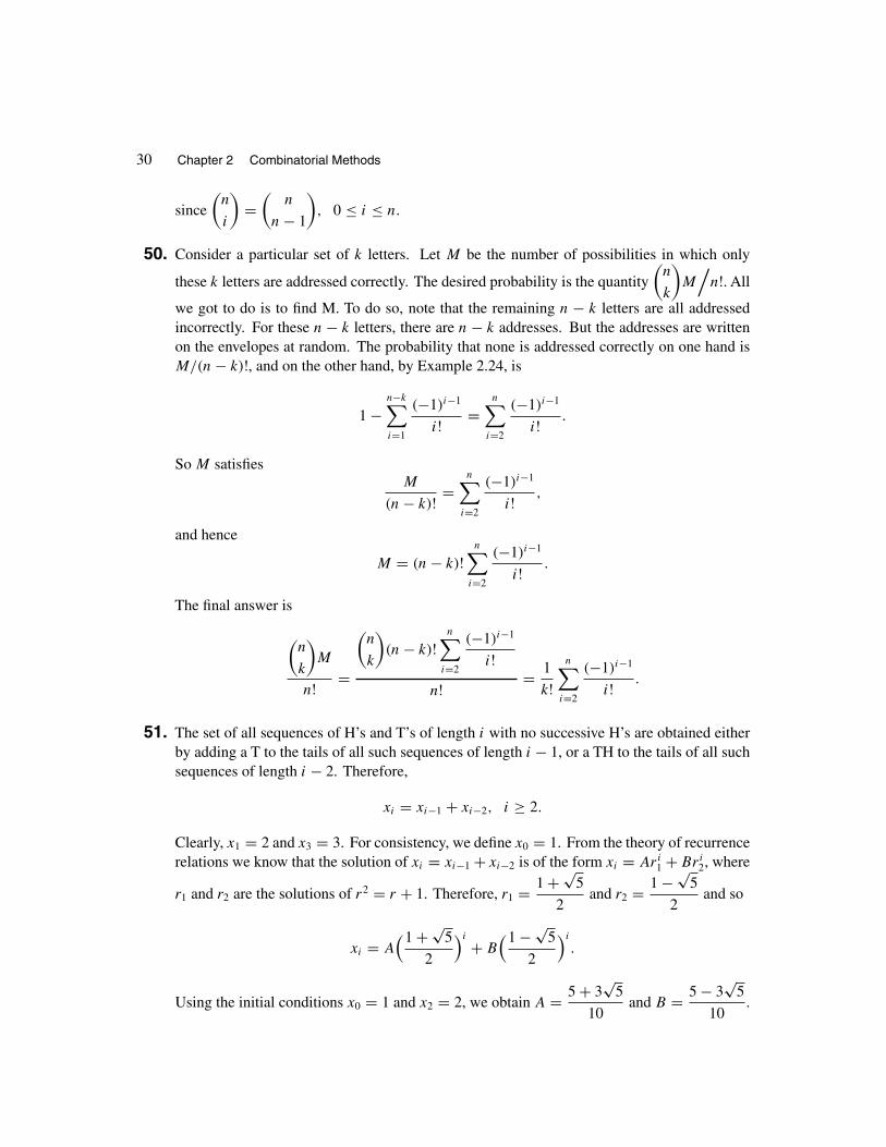
50. Consider a particular set of k letters. Let M be the number of possibilities in which only
these k letters are addressed correctly. The desired probability is the quantity
(n
k
)M/
n!. All
we got to do is to find M. To do so, note that the remaining n − k letters are all addressedincorrectly. For these n − k letters, there are n − k addresses. But the addresses are writtenon the envelopes at random. The probability that none is addressed correctly on one hand isM/(n − k)!, and on the other hand, by Example 2.24, is
1 −n−k∑i=1
(−1)i−1
i! =n∑
i=2
(−1)i−1
i! .
So M satisfiesM
(n − k)! =n∑
i=2
(−1)i−1
i! ,
and hence
M = (n − k)!n∑
i=2
(−1)i−1
i! .
The final answer is
(n
k
)M
n! =
(n
k
)(n − k)!
n∑i=2
(−1)i−1
i!n! = 1
k!n∑
i=2
(−1)i−1
i! .
51. The set of all sequences of H’s and T’s of length i with no successive H’s are obtained eitherby adding a T to the tails of all such sequences of length i − 1, or a TH to the tails of all suchsequences of length i − 2. Therefore,
xi = xi−1 + xi−2, i ≥ 2.
Clearly, x1 = 2 and x3 = 3. For consistency, we define x0 = 1. From the theory of recurrencerelations we know that the solution of xi = xi−1 + xi−2 is of the form xi = Ari
1 + Bri2, where
r1 and r2 are the solutions of r2 = r + 1. Therefore, r1 = 1 + √5
2and r2 = 1 − √
5
2and so
xi = A(1 + √
5
2
)i + B(1 − √
5
2
)i
.
Using the initial conditions x0 = 1 and x2 = 2, we obtain A = 5 + 3√
5
10and B = 5 − 3
√5
10.

Section 2.5 Stirling’s Formula 31
Hence the answer is
xn
2n = 1
2n
[(5 + 3√
5
10
)(1 + √5
2
)n +(5 − 3
√5
10
)(1 − √5
2
)n]= 1
10 × 22n
[(5 + 3
√5)(
1 + √5)n + (
5 − 3√
5)(
1 − √5)n]
.
52. For this exercise, a solution is given by Abramson and Moser in the October 1970 issue of theAmerican Mathematical Monthly.
2.5 STIRLING’s FORMULA
1. (a)(
2n
n
)1
22n= (2n)!
n! n!1
22n∼
√4πn (2n)2n e−2n
(2πn) n2n e−2n 22n∼ 1√
πn.
(b)
[(2n)!]3
(4n)! (n!)2∼
[√4πn (2n)2n e−2n
]3
√8πn (4n)4n e−4n (2πn) n2n e−2n
=√
2
4n.
REVIEW PROBLEMS FOR CHAPTER 2
1. The desired quantity is equal to the number of subsets of all seven varieties of fruit minus 1(the empty set); so it is 27 − 1 = 127.
2. The number of choices Virginia has is equal to the number of subsets of {1, 2, 5, 10, 20} minus1 (for empty set). So the answer is 25 − 1 = 31.
3. (6 × 5 × 4 × 3)/64 = 0.278.
4. 10/(10
2
)= 0.222.
5.9!
3! 2! 2! 2! = 7560.
6. 5!/5 = 4! = 24.
7. 3! · 4! · 4! · 4! = 82, 944.
8. 1 −
(23
6
)(
30
6
) = 0.83.

32 Chapter 2 Combinatorial Methods
9. Since the refrigerators are identical, the answer is 1.
10. 6! = 720.
11. (Draw a tree diagram.) In 18 out of 52 possible cases the tournament ends because John wins4 games without winning 3 in a row. So the answer is 34.62%.
12. Yes, it is because the probability of what happened is 1/72 = 0.02.
13. 9 8 = 43, 046, 721.
14. (a) 26 × 25 × 24 × 23 × 22 × 21 = 165, 765, 600;
(b) 26 × 25 × 24 × 23 × 22 × 5 = 39, 468, 000;
(c)(
5
2
)26
(3
1
)25
(2
1
)24
(1
1
)23 = 21, 528, 000.
15.
(6
3
)+(
6
1
)+(
6
1
)+(
6
1
)(2
1
)(2
1
)(
10
3
) = 0.467.
Another Solution:
(6
3
)+(
6
1
)(4
2
)(
10
3
) = 0.467.
16.8 × 4 ×6 P4
8P6= 0.571.
17. 1 − 278
288= 0.252.
18.(3!/3)(5!)3
15!/15= 0.000396.
19. 312 = 531, 441.
20.
(4
1
)(48
12
)(3
1
)(36
12
)(2
1
)(24
12
)(1
1
)(12
12
)52!
13! 13! 13! 13!= 0.1055.

Chapter 2 Review Problems 33
21. Let A1, A2, A3, and A4 be the events that there is no professor, no associate professor, noassistant professor, and no instructor in the committee, respectively. The desired probabilityis
P(Ac1A
c2A
c3A
c4) = 1 − P(A1 ∪ A2 ∪ A3 ∪ A4),
where P(A1 ∪ A2 ∪ A3 ∪ A4) is calculated using the inclusion-exclusion principle:
P(A1 ∪ A2 ∪ A3 ∪ A4) = P(A1) + P(A2) + P(A3) + P(A4)
− P(A1A2) − P(A1A3) − P(A1A4) − P(A2A3) − P(A2A4) − P(A3A4)
+ P(A1A2A3) + P(A1A3A4) + P(A1A2A4) + P(A2A3A4) − P(A1A2A3A4)
=[
1/(34
6
)][(28
6
)+(
28
6
)+(
24
6
)+(
22
6
)−(
22
6
)−(
18
6
)−(
16
6
)−(
18
6
)
−(
16
6
)−(
12
6
)+(
12
6
)+(
6
6
)+(
10
6
)+(
6
6
)− 0
]= 0.621.
Therefore, the desired probability equals 1 − 0.621 = 0.379.
22.(15!)2
30!/(2!)15= 0.0002112.
23. (N − n + 1)/(N
n
).
24. (a)
(4
2
)(48
24
)(
52
26
) = 0.390; (b)
(40
1
)(
52
13
) = 6.299 × 10⁻¹¹;
(c)
(13
5
)(39
8
)(8
8
)(31
5
)(
52
13
)(39
13
) = 0.00000261.
25. 12!/(3!)4 = 369, 600.
26. There is a one-to-one correspondence between all cases in which the eighth outcome obtainedis not a repetition and all cases in which the first outcome obtained will not be repeated. Theanswer is
6 × 5 × 5 × 5 × 5 × 5 × 5 × 5
6 × 6 × 6 × 6 × 6 × 6 × 6 × 6=(5
6
)7 = 0.279.
27. There are 9 × 103 = 9, 000 four-digit numbers. To count the number of desired four-digitnumbers, note that if 0 is to be one of the digits, then the thousands place of the number must be

34 Chapter 2 Combinatorial Methods
0, but this cannot be the case since the first digit of an n-digit number is nonzero. Keeping thisin mind, it must be clear that from every 4-combination of the set {1, 2, . . . , 9}, exactly onefour-digit number can be constructed in which its ones place is greater than its tens place, itstens place is greater than it hundreds place, and its hundreds place is greater than its thousands
place. Therefore, the number of such four-digit numbers is
(9
4
)= 126. Hence the desired
probability is = 0.014.
28. Since the sum of the digits of 100,000 is 1, we ignore 100,000 and assume that all of the numbershave five digits by placing 0’s in front of those with less than five digits. The following processestablishes a one-to-one correspondence between such numbers, d1d2d3d4d5,
∑5i=1 di = 8,
and placement of 8 identical objects into 5 distinguishable cells: Put d1 of the objects intothe first cell, d2 of the objects into the second cell, d3 into the third cell, and so on. Since
this can be done in
(8 + 5 − 1
5 − 1
)=(
12
8
)= 495 ways, the number of integers from the set
{1, 2, 3, . . . , 100000} in which the sum of the digits is 8 is 495. Hence the desired probabilityis 495/100, 000 = 0.00495.

Chapter 3
Conditional Probability
and Independence
3.1 CONDITIONAL PROBABILITY
1. P(W | U) = P(UW)
P (U)= 0.15
0.25= 0.60.
2. Let E be the event that in the blood of the randomly selected soldier A antigen is found. LetF be the event that the blood type of the soldier is A. We have
P(F | E) = P(FE)
P (E)= 0.41
0.41 + 0.04= 0.911.
3.0.20
0.32= 0.625.
4. The reduced sample space is{(1, 4), (2, 3), (3, 2), (4, 1), (4, 6), (5, 5), (6, 4)
}; therefore, the
desired probability is 1/7.
5.30 − 20
30 − 15= 2
3.
6. Both of the inequalities are equivalent to P(AB) > P(A)P (B).
7.1/3
(1/3) + (1/2)= 2
5.
8. 4/30 = 0.133.
36 Chapter 3 Conditional Probability and Independence
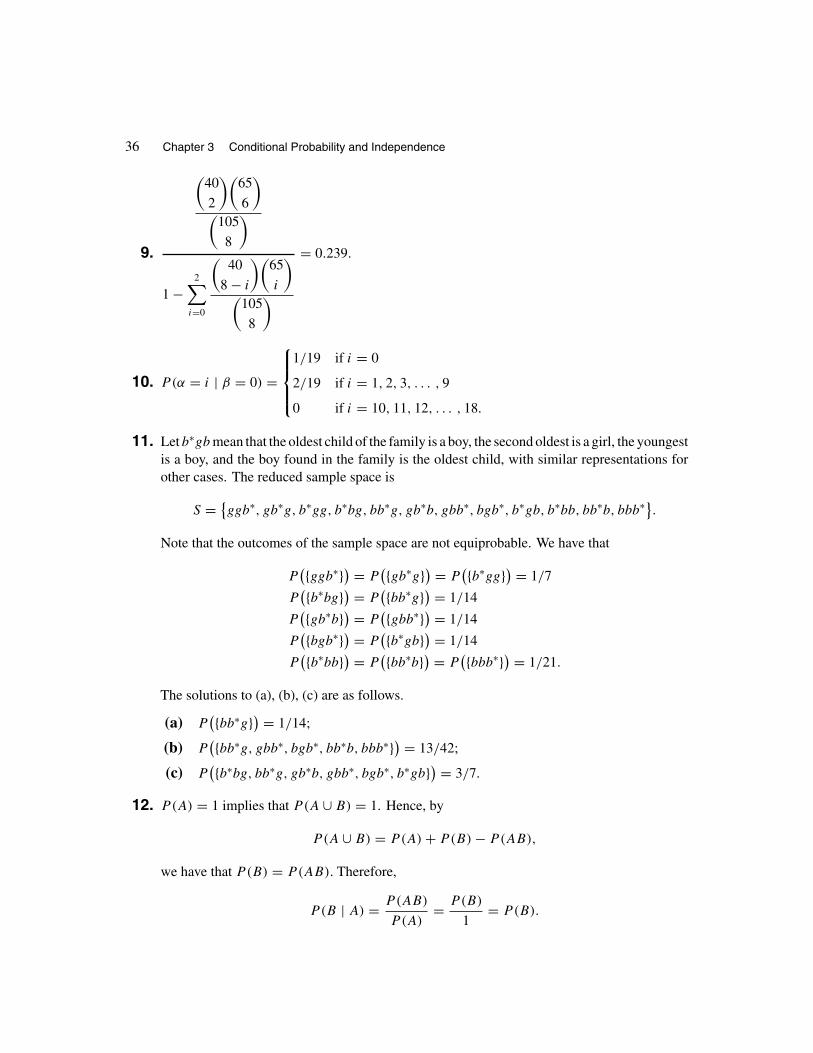
9.
(40
2
)(65
6
)(
105
8
)
1 −2∑
i=0
(40
8 − i
)(65
i
)(
105
8
)= 0.239.
10. P(α = i | β = 0) =
⎧⎪⎪⎨⎪⎪⎩1/19 if i = 0
2/19 if i = 1, 2, 3, . . . , 9
0 if i = 10, 11, 12, . . . , 18.
11. Let b∗gb mean that the oldest child of the family is a boy, the second oldest is a girl, the youngestis a boy, and the boy found in the family is the oldest child, with similar representations forother cases. The reduced sample space is
S = {ggb∗, gb∗g, b∗gg, b∗bg, bb∗g, gb∗b, gbb∗, bgb∗, b∗gb, b∗bb, bb∗b, bbb∗}.
Note that the outcomes of the sample space are not equiprobable. We have that
P({ggb∗}) = P
({gb∗g}) = P({b∗gg}) = 1/7
P({b∗bg}) = P
({bb∗g}) = 1/14
P({gb∗b}) = P
({gbb∗}) = 1/14
P({bgb∗}) = P
({b∗gb}) = 1/14
P({b∗bb}) = P
({bb∗b}) = P({bbb∗}) = 1/21.
The solutions to (a), (b), (c) are as follows.
(a) P({bb∗g}) = 1/14;
(b) P({bb∗g, gbb∗, bgb∗, bb∗b, bbb∗}) = 13/42;
(c) P({b∗bg, bb∗g, gb∗b, gbb∗, bgb∗, b∗gb}) = 3/7.
12. P(A) = 1 implies that P(A ∪ B) = 1. Hence, by
P(A ∪ B) = P(A) + P(B) − P(AB),
we have that P(B) = P(AB). Therefore,
P(B | A) = P(AB)
P (A)= P(B)
1= P(B).
Section 3.1 Conditional Probability 37
13. P(A | B) = P(AB)
b, where
P(AB) = P(A) + P(B) − P(A ∪ B) ≥ P(A) + P(B) − 1 = a + b − 1.
14. (a) P(AB) ≥ 0, P (B) > 0. Therefore, P(A | B) = P(AB)
P (B)≥ 0.
(b) P(S | B) = P(SB)
P (B)= P(B)
P (B)= 1.
(c) P( ∞⋃
i=1
Ai
∣∣∣ B)
=P
((⋃∞i=1 Ai
)B
)P(B)
=P(⋃∞
i=1 AiB)
P(B)
=
∞∑i=1
P(AiB)
P (B)=
∞∑i=1
P(AiB)
P (B)=
∞∑i=1
P(Ai | B).
Note that P(∪∞i=1AiB) = ∑∞
i=1 P(AiB), since mutual exclusiveness of Ai’s imply that ofAiB’s; i.e., AiAj = ∅, i �= j , implies that (AiB)(AjB) = ∅, i �= j .
15. The given inequalities imply that P(EF) ≥ P(GF) and P(EF c) ≥ P(GFc). Thus
P(E) = P(EF) + P(EF c) ≥ P(GF) + P(GFc) = P(G).
16. Reduce the sample space: Marlon chooses from six dramas and seven comedies two at random.
What is the probability that they are both comedies? The answer is
(7
2
)/(13
2
)= 0.269.
17. Reduce the sample space: There are 21 crayons of which three are red. Seven of these crayonsare selected at random and given to Marty. What is the probability that three of them are red?
The answer is
(18
4
)/(21
7
)= 0.0263.
18. (a) The reduced sample space is S = {1, 3, 5, 7, 9, . . . , 9999}. There are 5000 elements inS. Since the set {5, 7, 9, 11, 13, 15, . . . , 9999} includes exactly 4998/3 = 1666 odd numbersthat are divisible by three, the reduced sample space has 1667 odd numbers that are divisibleby 3. So the answer is 1667/5000 = 0.3334.
(b) Let O be the event that the number selected at random is odd. Let F be the event that it isdivisible by 5 and T be the event that it is divisible by 3. The desired probability is calculatedas follows.
P(F cT c | O) = 1 − P(F ∪ T | O) = 1 − P(F | O) − P(T | O) + P(FT | O)
= 1 − 1000
5000− 1667
5000+ 333
5000= 0.5332.

38 Chapter 3 Conditional Probability and Independence
19. Let A be the event that during this period he has hiked in Oregon Ridge Park at least once. LetB be the event that during this period he has hiked in this park at least twice. We have
P(B | A) = P(B)
P (A),
where
P(A) = 1 − 510
610= 0.838
and
P(B) = 1 − 510
610− 10 × 59
610= 0.515.
So the answer is 0.515/0.838 = 0.615.
20. The numbers of 333 red and 583 blue chips are divisible by 3. Thus the reduced sample spacehas 333 + 583 = 916 points. Of these numbers, [1000/15] = 66 belong to red balls andare divisible by 5 and [1750/15] = 116 belong to blue balls and are divisible by 5. Thus thedesired probability is 182/916 = 0.199.
21. Reduce the sample space: There are two types of animals in a laboratory, 15 type I and 13type II. Six animals are selected at random; what is the probability that at least two of themare Type II? The answer is
1 −
(15
6
)+(
13
1
)(15
5
)(
28
6
) = 0.883.
22. Reduce the sample space: 30 students of which 12 are French and nine are Korean are dividedrandomly into two classes of 15 each. What is the probability that one of them has exactlyfour French and exactly three Korean students? The solution to this problem is(
12
4
)(9
3
)(9
8
)(
30
15
)(15
15
) = 0.00241.
23. This sounds puzzling because apparently the only deduction from the name “Mary” is that oneof the children is a girl. But the crucial difference between this and Example 3.2 is reflectedin the implicit assumption that both girls cannot be Mary. That is, the same name cannot beused for two children in the same family. In fact, any other identifying feature that cannot beshared by both girls would do the trick.

Section 3.2 Law of Multiplication 39
3.2 LAW OF MULTIPLICATION
1. Let G be the event that Susan is guilty. Let L be the event that Robert will lie. The probabilitythat Robert will commit perjury is
P(GL) = P(G)P (L | G) = (0.65)(0.25) = 0.1625.
2. The answer is11
14× 10
13× 9
12× 8
11× 7
10× 6
9= 0.15.
3. By the law of multiplication, the answer is
52
52× 50
51× 48
50× 46
49× 44
48× 42
47= 0.72.
4. (a)8
20× 7
19× 6
18× 5
17= 0.0144;
(b)8
20× 7
19× 12
18+ 8
20× 12
19× 7
18+ 12
20× 8
19× 7
18+ 8
20× 7
19× 6
18= 0.344.
5. (a)6
11× 5
10× 5
9× 4
8× 4
7× 3
6× 3
5× 2
4× 2
3× 1
2× 1
1= 0.00216.
(b)5
11× 4
10× 3
9× 2
8× 1
7= 0.00216.
6.3
8× 5
10× 5
13× 8
15+ 5
8× 3
11× 8
13× 5
16= 0.0712.
7. Let Ai be the event that the ith person draws the “you lose” paper. Clearly,
P(A1) = 1
200,
P (A2) = P(Ac1A2) = P(Ac
1)P (A2 | Ac1) = 199
200· 1
199= 1
200,
P (A3) = P(Ac1A
c2A3) = P(Ac
1)P (Ac2 | Ac
1)P (A3 | Ac1A
c2) = 199
200· 198
199· 1
198= 1
200,
and so on. Therefore, P(Ai) = 1/200 for 1 ≤ i ≤ 200. This means that it makes no differenceif you draw first, last or anywhere in the middle. Here is MarilynVos Savant’s intuitive solutionto this problem:

40 Chapter 3 Conditional Probability and Independence
It makes no difference if you draw first, last, or anywhere in the middle. Look at itthis way: Say the robbers make everyone draw at once. You’d agree that everyonehas the same change of losing (one in 200), right? Taking turns just makes thatsame event happen in a slow and orderly fashion. Envision a raffle at a church with200 people in attendance, each person buys a ticket. Some buy a ticket when theyarrive, some during the event, and some just before the winner is drawn. It doesn’tmatter. At the party the end result is this: all 200 guests draw a slip of paper, and,regardless of when they look at the slips, the result will be identical: one will lose.You can’t alter your chances by looking at your slip before anyone else does, orwaiting until everyone else has looked at theirs.
8. Let B be the event that a randomly selected person from the population at large has poor creditreport. Let I be the event that the person selected at random will improve his or her creditrating within the next three years. We have
P(B | I ) = P(BI)
P (I)= P(I | B)P (B)
P (I)= (0.30)(0.18)
0.75= 0.072.
The desired probability is 1−0.072 = 0.928. Therefore, 92.8% of the people who will improvetheir credit records within the next three years are the ones with good credit ratings.
9. For 1 ≤ n ≤ 39, let En be the event that none of the first n − 1 cards is a heart or the aceof spades. Let Fn be the event that the nth card drawn is the ace of spades. Then the eventof “no heart before the ace of spades” is
⋃39n=1 EnFn. Clearly, {EnFn, 1 ≤ n ≤ 39} forms a
sequence of mutually exclusive events. Hence
P( 39⋃
n=1
EnFn
)=
39∑n=1
P(EnFn) =39∑
n=1
P(En)P (Fn | En)
=39∑
n=1
(38
n − 1
)(
52
n − 1
) × 1
53 − n= 1
14,
a result which is not unexpected.
10. P(F)P (E | F) =
(13
3
)(39
6
)(
52
9
) × 10
43= 0.059.
11. By the law of multiplication,
P(An) = 2
3× 3
4× 4
5× · · · × n + 1
n + 2= 2
n + 2.

Section 3.3 Law of Total Probability 41
Now since A1 ⊇ A2 ⊇ A3 ⊇ · · · ⊇ An ⊇ An+1 ⊇ · · · , by Theorem 1.8,
P( ∞⋂
i=1
Ai
)= lim
n→∞ P(An) = 0.
3.3 LAW OF TOTAL PROBABILITY
1.1
2× 0.05 + 1
2× 0.0025 = 0.02625.
2. (0.16)(0.60) + (0.20)(0.40) = 0.176.
3.1
3(0.75) + 1
3(0.68) + 1
3(0.47) = 0.633.
4.12
51× 13
52+ 13
51× 39
52= 1
4.
5.11
50×
(13
2
)(
52
2
) + 12
50×
(13
1
)(39
1
)(
52
2
) + 13
50×
(39
2
)(
52
2
) = 1
4.
6. (0.20)(0.40) + (0.35)(0.60) = 0.290.
7. (0.37)(0.80) + (0.63)(0.65) = 0.7055.
8.1
6(0.6) + 1
6(0.5) + 1
6(0.7) + 1
6(0.9) + 1
6(0.7) + 1
6(0.8) = 0.7.
9. (0.50)(0.04) + (0.30)(0.02) + (0.20)(0.04) = 0.034.
10. Let B be the event that the randomly selected child from the countryside is a boy. Let E bethe event that the randomly selected child is the first child of the family and F be the eventthat he or she is the second child of the family. Clearly, P(E) = 2/3 and P(F) = 1/3. Bythe law of total probability,
P(B) = P(B | E)P (E) + P(B | F)P (F ) = 1
2× 2
3+ 1
2× 1
3= 1
2.
Therefore, assuming that sex distributions are equally probable, in the Chinese countryside,the distribution of sexes will remain equal. Here is Marilyn Vos Savant’s intuitive solution tothis problem:

42 Chapter 3 Conditional Probability and Independence
The distribution of sexes will remain roughly equal. That’s because–no matter howmany or how few children are born anywhere, anytime, with or without restriction–half will be boys and half will be girls: Only the act of conception (not the govern-ment!) determines their sex.
One can demonstrate this mathematically. (In this example, we’ll assume thatwomen with firstborn girls will always have a second child.) Let’s say 100 womengive birth, half to boys and half to girls. The half with boys must end their families.There are now 50 boys and 50 girls. The half with girls (50) give birth again, halfto boys and half to girls. This adds 25 boys and 25 girls, so there are now 75 boysand 75 girls. Now all must end their families. So the result of the policy is that therewill be fewer children in number, but the boy/girl ratio will not be affected.
11. The probability that the first person gets a gold coin is 3/5. The probability that the secondperson gets a gold coin is
2
4× 3
5+ 3
4× 2
5= 3
5.
The probability that the third person gets a gold coin is
3
5× 2
4× 1
3+ 3
5× 2
4× 2
3+ 2
5× 3
4× 2
5+ 2
5× 1
4× 3
3= 3
5,
and so on. Therefore, they are all equal.
12. A Probabilistic Solution: Let n be the number of adults in the town. Let x be the numberof men in the town. Then n − x is the number of women in the town. Since the number ofmarried men and married women are equal, we have
x · 7
9= (n − x) · 3
5.
This relation implies that x = (27/62)n. Therefore, the probability that a randomly selectedadult is male is (27/62)n
/n = 27/62. The probability that a randomly selected adult is female
is 1 − (27/62) = 35/62. Let A be the event that a randomly selected adult is married. Let M
be the event that the randomly selected adult is a man, and let W be the event that the randomlyselected adult is a woman. By the law of total probability,
P(A) = P(A | M)P(M) + P(A | W)P (W)
= 7
9· 27
62+ 3
5· 35
62= 42
62= 21
31≈ 0.677.
Therefore, 21/31st of the adults are married.
An Arithmetical Solution: The common numerator of the two fractions is 21. Hence21/27th of the men and 21/35th of the women are married. We find the common numeratorbecause the number of married men and the number of married women are equal. This showsthat of every 27 + 35 = 62 adults, 21 + 21 = 42 are married. Hence 42/62th = 21/31st of theadults in the town are married.

Section 3.3 Law of Total Probability 43
13. The answer is clearly 0.40. This can also be computed from
(0.40)(0.75) + (0.40)(0.25) = 0.40.
14. Let A be the event that a randomly selected child is the kth born of his or her family. Let Bj
be the event that he or she is from a family with j children. Then
P(A) =c∑
j=k
P (A | Bj)P (Bj ),
where, clearly, P(A | Bj) = 1/j . To find P(Bj), note that there are αiN families with j
children. Therefore, the total number of children in the world is∑c
i=0 i(αiN) of which j (Nαj )
are from families with j children. Hence
P(Bj) = j (Nαj )∑ci=0 i(αiN)
= jαj∑ci=0 iαi
.
This shows that the desired fraction is given by
P(A) =c∑
j=k
P (A | Bj)P (Bj ) =c∑
j=k
1
j· jαj∑c
i=0 iαi
=c∑
j=k
αj∑ci=0 iαi
=∑c
j=k αj∑ci=0 iαi
.
15. Q(E | F) = Q(EF)
Q(F)= P(EF | B)
P (F | B)=
P(EFB)
P (B)
P (FB)
P (B)
= P(EFB)
P (FB)= P(E | FB).
16. Let M , C, and F denote the events that the random student is married, is married to a studentat the same campus, and is female, respectively. We have that
P(F | M) = P(F | MC)P (C | M)+P(F | MCc)P (Cc | M) = (0.40)1
3+(0.30)
2
3= 0.333.
17. Let p(k, n) be the probability that exactly k of the first n seeds planted in the farm germinated.Using induction on n, we will show that p(k, n) = 1/(n − 1) for all k < n. For n = 2,p(1, 2) = 1 = 1/(2 − 1) is true. If p(k, n − 1) = 1/(n − 2) for all k < n − 1, then, by thelaw of total probability,
p(k, n) = k − 1
n − 1p(k − 1, n − 1) + n − k − 1
n − 1p(k, n − 1)
= k − 1
n − 1· 1
n − 2+ n − k − 1
n − 1· 1
n − 2= 1
n − 1.
This proves the induction hypothesis.

44 Chapter 3 Conditional Probability and Independence
18. Reducing the sample space, we have that the answer is 7/10.
19.
(8
3
)(
18
3
) ×
(10
3
)(
18
3
) +
(7
3
)(
18
3
) ×
(10
2
)(8
1
)(
18
3
) +
(6
3
)(
18
3
) ×
(10
1
)(8
2
)(
18
3
) +
(5
3
)(
18
3
) ×
(8
3
)(
18
3
) = 0.0383.
20. We have that
P(A | G) = P(A | GO)P (O | G) + P(A | GM)P (M | G) + P(A | GY)P (Y | G)
= 0 × 1
3+ 1
2× 1
3+ 3
4× 1
3= 5
12.
21. Let E be the event that the third number falls between the first two. Let A be the event thatthe first number is smaller than the second number. We have that
P(E | A) = P(EA)
P (A)= 1/6
1/2= 1
3.
Intuitively, the fact that P(A) = 1/2 and P(EA) = 1/6 should be clear (say, by symmetry).However, we can prove these rigorously. We show that P(A) = 1/2; P(EA) = 1/6 can beproved similarly. Let B be the event that the second number selected is smaller than the firstnumber. Clearly A = Bc and we only need to show that P(B) = 1/2. To do this, let Bi bethe event that the first number drawn is i, 1 ≤ i ≤ n. Since {B1, B2, . . . , Bn} is a partition ofthe sample space,
P(B) =n∑
i=1
P(B | Bi)P (Bi).
Now P(B | B1) = 0 because if the first number selected is 1, the second number selected
cannot be smaller. P(B | Bi) = i − 1
n − 1, 1 ≤ i ≤ n since if the first number is i, the second
number must be one of 1, 2, 3, . . . , i − 1 if it is to be smaller. Thus
P(B) =n∑
i=1
P(B | Bi)P (Bi) =n∑
i=2
i − 1
n − 1· 1
n= 1
(n − 1)n
n∑i=2
(i − 1)
= 1
(n − 1)n
[1 + 2 + 3 + · · · + (n − 1)
] = 1
(n − 1)n· (n − 1)n
2= 1
2.
22. Let Em be the event that Avril selects the best suitor given her strategy. Let Bi be the eventthat the best suitor is the ith of Avril’s dates. By the law of total probability,
P(Em) =n∑
i=1
P(Em | Bi)P (Bi) = 1
n
n∑i=1
P(Em | Bi).

Section 3.3 Law of Total Probability 45
Clearly, P(Em | Bi) = 0 for 1 ≤ i ≤ m. For i > m, if the ith suitor is the best, then Avrilchooses him if and only if among the first i − 1 suitors Avril dates, the best is one of the firstm. So
P(Em | Bi) = m
i − 1.
Therefore,
P(Em) = 1
n
n∑i=m+1
m
i − 1= m
n
n∑i=m+1
1
i − 1.
Nown∑
i=m+1
1
i − 1≈∫ n
m
1
xdx = ln
( n
m
).
ThusP(Em) ≈ m
nln( n
m
).
To find the maximum of P(Em), consider the differentiable function
h(x) = x
nln(n
x
).
Since
h′(x) = 1
nln(n
x
)− 1
n= 0
implies that x = n/e, the maximum of P(Em) is at m = [n/e], where [n/e] is the greatestinteger less than or equal to n/e. Hence Avril should dump the first [n/e] suitors she datesand marry the first suitor she dates afterward who is better than all those preceding him. Theprobability that with such a strategy she selects the best suitor of all n is approximately
h(n
e
)= 1
eln e = 1
e≈ 0.368.
23. Let N be the set of nonnegative integers. The domain of f is{(g, r) ∈ N × N : 0 ≤ g ≤ N, 0 ≤ r ≤ N, 0 < g + r < 2N
}.
Extending the domain of f to all points (g, r) ∈ R × R, we find that∂f
∂g= ∂f
∂r= 0 gives
g = r = N/2 and f (N/2, N/2) = 1/2. However, this is not the maximum value because onthe boundary of the domain of f along r = 0, we find that
f (g, 0) = 1
2
(1 + N − g
2N − g
)is maximum at g = 1 and
f (1, 0) = 1
2
(3N − 2
2N − 1
)≥ 1
2.

46 Chapter 3 Conditional Probability and Independence
We also find that on the boundary along r = N ,
f (g, N) = 1
2
( g
g + N+ 1
)is maximum at g = N − 1 and
f (N − 1, N) = 1
2
(3N − 2
2N − 1
)≥ 1
2.
The maximums of f along other sides of the boundary are all less than1
2
(3N − 2
2N − 1
). Therefore,
there are exactly two maximums and they occur at (1, 0) and (N−1, N). That is, the maximumof f occurs if one urn contains one green and 0 red balls and the other one contains N −1 green
and N red balls. For large N , the probability that the prisoner is freed is1
2
(3N − 2
2N − 1
)≈ 3
4.
3.4 BAYES’ FORMULA
1.(3/4)(0.40)
(3/4)(0.40) + (1/3)(0.60)= 3
5.
2.1(2/3)
1(2/3) + (1/4)(1/3)= 8
9.
3. Let G and I be the events that the suspect is guilty and innocent, respectively. Let A be theevent that the suspect is left-handed. Since {G, I } is a partition of the sample space, we canuse Bayes’ formula to calculate P(G | A), the probability that the suspect has committed thecrime in view of the new evidence.
P(G | A) = P(A | G)P (G)
P (A | G)P (G) + P(A | I )P (I)= (0.85)(0.65)
(0.85)(0.65) + (0.23)(0.35)≈ 0.87.
4. Let G be the event that Susan is guilty. Let C be the event that Robert and Julie give conflictingtestimony. By Bayes’ formula,
P(G | C) = P(C | G)P (G)
P (C | G)P (G) + P(C | Gc)P (Gc)= (0.25)(0.65)
(0.25)(0.65) + (0.30)(0.35)= 0.607.
5.(0.02)(0.30)
(0.02)(0.30) + (0.05)(0.70)= 0.1463.
6.
[(6
3
)/(11
3
)](1
2
)[(
6
3
)/(11
3
)](1
2
)+ 1
(1
2
) = 4
37.

Section 3.4 Bayes’ Formula 47
7.(0.92)(1/5000)
(0.92)(1/5000) + (1/500)(4999/5000)= 0.084.
8. Let A be the event that two of the three coins are dimes. Let B be the event that the coinselected from urn I is a dime. Then
P(B | A) = P(A | B)P (B)
P (A | B)P (B) + P(A | Bc)P (Bc)=
(5
7· 3
4+ 2
7· 1
4
)4
7(5
7· 3
4+ 2
7· 1
4
)4
7+(5
7· 1
4
)3
7
= 68
83.
9.(0.15)(0.25)
(0.15)(0.25) + (0.85)(0.75)= 0.056.
10. Let R be the event that the upper side of the card selected is red. Let BB be the event that thecard with both sides black is selected. Define RR and RB similarly. By Bayes’ Formula,
P(RB | R) = P(R | RB)P (RB)
P (R | RB)P (RB) + P(R | RR)P (RR) + P(R | BB)P (BB)
= (1/2)(1/3)
(1/2)(1/3) + 1(1/3) + 0(1/3)= 1
3.
11.1(1
6
)5∑
i=0
[(1000 − i
100
)/(1000
100
)](1
6
) = 0.21.
12. Let A be the event that the wallet originally contained a $2 bill. Let B be the event that thebill removed is a $2 bill. The desired probability is given by
P(A | B) = P(B | A
)P(A)
P(B | A
)P(A) + P
(B | Ac
)P(Ac)
=1 × 1
2
1 × 1
2+ 1
2× 1
2
= 2
3.
13. By Bayes’ formula, the probability that the horse that comes out is from stable I equals
(20/33)(1/2)
(20/33)(1/2) + (25/33)(1/2)= 4
9.
The probability that it is from stable II is 5/9; hence the desired probability is
20
33· 4
9+ 25
33· 5
9= 205
297= 0.69.

48 Chapter 3 Conditional Probability and Independence
14.
2
4·
(5
2
)(3
2
)(
8
4
)
0 ·
(5
4
)(
8
4
) + 1
4·
(5
3
)(3
1
)(
8
4
) + 2
4·
(5
2
)(3
2
)(
8
4
) + 3
4·
(5
1
)(3
3
)(
8
4
)= 0.571.
15. Let I be the event that the person is ill with the disease, N be the event that the result of thetest on the person is negative, and R denote the event that the person has the rash. We areinterested in P(I | R):
P(I | R) = P(IN | R) + P(INc | R) = 0 + P(INc | R).
Since {IN, INc, I cN, I cNc} is a partition of the sample space, by Bayes’ Formula,
P(I | R) = P(INc | R)
= P(R | INc)P (INc)
P (R | IN)P (IN) + P(R | INc)P (INc) + P(R | I cN)P (I cN) + P(R | I cNc)P (I cNc)
= (0.2)(0.30 × 0.90)
0(0.30 × 0.10) + (0.2)(0.30 × 0.90) + 0(0.70 × 0.75) + (0.2)(0.70 × 0.25)= 0.61.
3.5 INDEPENDENCE
1. No, because by independence, regardless of the number of heads that have previously occurred,the probability of tails remains to be 1/2 on each flip.
2. A and B are mutually exclusive; therefore, they are dependent. If A occurs, then the probabilitythat B occurs is 0 and vice versa.
3. Neither. Since the probability that a fighter plane returns from a mission without mishap is49/50 independent of other missions, the probability that a pilot who flew 49 consecutivemissions without mishap making another successful flight is still 49/50=0.98; neither highernor lower than the probability of success in any other mission.
4. P(AB) = 1/12 = (1/2)(1/6); so A and B are independent.
5. (3/8)3(5/8)5 = 0.00503.
6. (3/4)2 = 0.5625.

Section 3.5 Independence 49
7. (a) (0.725)2 = 0.526; (b) (1 − 0.725)2 = 0.076.
8. Suppose that for an event A, P(A) = 3/4. Then the probability that A occurs in two con-secutive independent experiments is 9/16. So the correct odds are 9 to 7, not 9 to 1. In latercomputations, Cardano, himself, had realized that the correct answer is 9 to 7 and not 9 to 1.
9. We have that
P(A beats B) = P(A rolls 4) = 4
6,
P (B beats A) = 1 − P(A beats B) = 1 − 4
6= 2
6,
P (B beats C) = P(C rolls 2) = 4
6,
P (C beats B) = 1 − P(B beats C) = 1 − 4
6= 2
6,
P (C beats D) = P(C rolls 6) + P(C rolls 2 and D rolls 1) = 2
6+ 4
6× 3
6= 4
6,
P (D beats C) = 1 − P(C beats D) = 1 − 4
6= 2
6,
P (D beats A) = P(D rolls 5) + P(D rolls 1 and A rolls 0) = 3
6+ 3
6× 2
6= 4
6.
10. For 1 ≤ i ≤ 4, let Ai be the event of obtaining 6 on the ith toss. Chevalier de Méré hadimplicitly thought that Ai’s are mutually exclusive and so
P(A1 ∪ A2 ∪ A3 ∪ A4
) = 1
6+ 1
6+ 1
6+ 1
6= 4 × 1
6.
Clearly Ai’s are not mutually exclusive. The correct answers are 1 − (5/6)4 = 0.5177 and1 − (35/36)24 = 0.4914.
11. (1 − 0.0001)64 = 0.9936.
12. In the experiment of tossing a coin, let A be the event of obtaining heads and B be the eventof obtaining tails.
13. (a) P(A ∪ B) ≥ P(A) = 1, so P(A ∪ B) = 1. Now
1 = P(A ∪ B) = P(A) + P(B) − P(AB) = 1 + P(B) − P(AB)
gives P(B) = P(AB).
(b) If P(A) = 0, then P(AB) = 0; so P(AB) = P(A)P (B) is valid. If P(A) = 1, bypart (a), P(AB) = P(B) = P(A)P (B).
14. P(AA) = P(A)P (A) implies that P(A) = [P(A)
]2. This gives P(A) = 0 or P(A) = 1.

50 Chapter 3 Conditional Probability and Independence
15. P(AB) = P(A)P (B) implies that P(A) = P(A)P (B). This gives P(A)[1 − P(B)
] = 0;so P(A) = 0 or P(B) = 1.
16. 1 − (0.45)6 = 0.9917.
17. 1 − (0.3)(0.2)(0.1) = 0.994.
18. There are(100 × 10 9) × (300 × 10 9) − 1 = 30 × 10 21 − 1
other stars in the universe. Provided that Aczel’s estimate is correct, the probability of no lifein orbit around any one given star in the known universe is
0.99999999999995
independently of other stars. Therefore, the probability of no life in orbit around any otherstar is
(0.99999999999995)30,000,000,000,000,000,000,000 −1.
Using Aczel’s words, “this number is indistinguishable from 0 at any level of decimal accuracyreported by the computer.” Hence the probability that there is life in orbit around at least oneother star is 1 for all practical purposes. If there were only a billion galaxies each having 10billion stars, still the probability of life would have been indistinguishable from 1.0 at any levelof accuracy reported by the computer. In fact, if we divide the stars into mutually exclusivegroups with each group containing billions of stars, then the argument above and Exercise 8of Section 1.7 imply that the probability of life in orbit around many other stars is a numberpractically indistinguishable from 1.
19. 1 − (0.94)15 − 15(0.94)14(0.06) = 0.226.
20. A and B are independent if and only if P(AB) = P(A)P (B), or, equivalently, if and only if
m
M + W= M
M + W· m + w
M + W.
This implies that m/M = w/W. Therefore, A and B are independent if and only if the fractionof the men who smoke is equal to the fraction of the women who smoke.
21. (a) By Theorem 1.6,
P(A(B ∪ C)
) = P(AB ∪ AC) = P(AB) + P(AC) − P(ABC)
= P(A)P (B) + P(A)P (C) − P(A)P (B)P (C)
= P(A)[P(B) + P(C) − P(B)P (C)
] = P(A)P (B ∪ C).
(b) P((A − B)C
) = P(ABcC) = P(A)P (Bc)P (C) = P(ABc)P (C) = P(A − B)P (C).
22. 1 − (5/6)6 = 0.6651.

Section 3.5 Independence 51
23. (a) 1 − [(n − 1)/n
]n. (b) As n → ∞, this approaches 1 − (1/e) = 0.6321.
24.1 − (0.85)10 − 10(0.85)9(0.15)
1 − (0.85)10= 0.567.
25. No. In the experiment of choosing a random number from (0, 1), let A, B, and C denote theevents that the point lies in (0, 1/2), (1/4, 3/4), and (1/2, 1), respectively.
26. Denote a family with two girls and one boy by ggb, with similar representations for othercases. The sample space is S = {ggg, bbb, ggb, gbb}. we have
P({ggg}) = P
({bbb}) = 1/8, P({ggb}) = P
({gbb}) = 3/8.
Clearly, P(A) = 6/8 = 3/4, P(B) = 4/8 = 1/2, and P(AB) = 3/8. Since P(AB) =P(A)P (B), the events A and B are independent. Using the same method, we can show thatfor families with two children and for families with four children, A and B are not independent.
27. If p is the probability of its occurrence in one trial, 1 − (1 − p)4 = 0.59. This implies thatp = 0.2.
28. (a) 1 − (1 − p1)(1 − p2) · · · (1 − pn). (b) (1 − p1)(1 − p2) · · · (1 − pn).
29. Let Ei be the event that the switch located at i is closed. The desired probability is
P(E1E2E4E6∪E1E3E5E6) = P(E1E2E4E6)+P(E1E3E5E6)−P(E1E2E3E4E5E6) = 2p4−p6.
30.(
5
3
)(2
3
)3(1
3
)2 = 0.329.
31. For n = 3, the probabilities of the given events, respectively, are(3
2
)(1
2
)2(1
2
)+(1
2
)3 = 1
2,
and (3
1
)(1
2
)(1
2
)2 +(
3
2
)(1
2
)2(1
2
)= 3
4.
The probability of their joint occurrence is(3
2
)(1
2
)2(1
2
)= 3
8= 1
2· 3
4.
So the given events are independent. For n = 4, similar calculations show that the givenevents are not independent.

52 Chapter 3 Conditional Probability and Independence
32. (a) 1 − (1/2)n. (b)(
n
k
)(1
2
)n
.
(c) Let An be the event of getting n heads in the first n flips. We have
A1 ⊇ A2 ⊇ A3 ⊇ · · · ⊇ An ⊇ An+1 ⊇ · · · .
The event of getting heads in all of the flips indefinitely is⋂∞
n=1 An. By the continuity propertyof probability function (Theorem 1.8), its probability is
P( ∞⋂
n=1
An
)= lim
n→∞ P(An) = limn→∞
(1
2
)n = 0.
33. Let Ai be the event that the sixth sum obtained is i, i = 2, 3, . . . , 12. Let B be the event thatthe sixth sum obtained is not a repetition. By the law of total probability,
P(B) =12∑i=2
P(B | Ai)P (Ai).
Note that in this sum, the terms for i = 2 and i = 12 are equal. This is true also for the termsfor i = 3 and 11, for the terms for i = 4 and 10, for the terms for i = 5 and 9, and for theterms for i = 6 and 8. So
P(B) = 2[ 6∑
i=2
P(B | Ai)P (Ai)]
+ P(B | A7)P (A7)
= 2[(35
36
)5( 1
36
)+(34
36
)5( 2
36
)+(33
36
)5( 3
36
)+(32
36
)5( 4
36
)+(31
36
)5( 5
36
)]+(30
36
)5( 6
36
)= 0.5614.
34. (a) Let E be the event that Dr. May’s suitcase does not reach his destination with him. Wehave
P(E) = (0.04) + (0.96)(0.05) + (0.96)(0.95)(0.05) + (0.96)(0.95)(0.95)(0.04) = 0.168,
or simply, P(E) = 1 − (0.96)(0.95)(0.96) = 0.168.
(b) Let D be the event that the suitcase is lost in Da Vinci airport in Rome. Then, by Bayes’formula,
P(D | E) = P(D)
P (E)= (0.96)(0.05)
0.168= 0.286.
35. Let E be the event of obtaining heads on the coin before an ace from the cards. Let H , T , A,and N denote the events of heads, tails, ace, and not ace in the first experiment, respectively.We use two different techniques to solve this problem.

Section 3.5 Independence 53
Technique 1: By the law of total probability,
P(E) = P(E | H)P (H) + P(E | T )P (T ) = 1 · 1
2+ P(E | T ) · 1
2,
where
P(E | T ) = P(E | T A)P (A | T ) + P(E | T N)P (N | T ) = 0 · 1
13+ P(E) · 12
13.
Thus
P(E) = 1
2+[P(E)
12
13
] 1
2,
which gives P(E) = 13/14.
Technique 2: We have that
P(E) = P(E | HA)P (HA)+P(E | T A)P (T A)+P(E | HN)P (HN)+P(E | T N)P (T N).
Thus
P(E) = 1 × 1
2× 1
13+ 0 × 1
2× 1
13+ 1 × 1
2× 12
13+ P(E) × 1
2× 12
13.
This gives P(E) = 13/14.
36. Let P(A) = p and P(B) = q. Let An be the event that none of A and B occurs in the firstn − 1 trials and the outcome of the nth experiment is A. The desired probability is
P( ∞⋃
n=1
An
)=
∞∑n=1
P(An) =∞∑
n=1
(1 − p − q)n−1p = p
1 − (1 − p − q)= p
p + q.
37. The probability of sum 5 is 1/9 and the probability of sum 7 is 1/6. Therefore, by the result of
Exercise 36, the desired probability is1/9
1/6 + 1/9= 2/5.
38. Let A be the event that one of them is red and the other one is blue. Let RB represent theevent that the ball drawn from urn I is red and the ball drawn form urn II is blue, with similarrepresentations for RR, BB, and BR. We have that
P(A) = P(A | RB)P (RB) + P(A | RR)P (RR) + P(A | BB)P (BB) + P(A | BR)P (BR)
=
(9
1
)(5
1
)(
14
2
) ( 9
10· 5
6
)+
(8
1
)(6
1
)(
14
2
) ( 9
10· 1
6
)+
(10
1
)(4
1
)(
14
2
) ( 1
10· 5
6
)+
(9
1
)(5
1
)(
14
2
) ( 1
10· 1
6
)
= 0.495.

54 Chapter 3 Conditional Probability and Independence
39. For convenience, let p0 = 0; the desired probability is
1 −n∏
i=1
(1 − pi) −n∑
i=1
(1 − p1)(1 − p2) · · · (1 − pi−1)pi(1 − pi+1) · · · (1 − pn).
40. Let p be the probability that a randomly selected person was born on one of the first 365 days;then 365p + (p/4) = 1 implies that p = 4/1461. Let E be the event that exactly four peopleof this group have the same birthday and that all the others have different birthdays. E is theunion of the following three mutually exclusive events:
F : Exactly four people of this group have the same birthday, all the others have differentbirthdays, and none of the birthdays is on the 366th day.
G: Exactly four people of this group have the same birthday, all the others have differentbirthdays, and exactly one has his/her birthday on the 366th day.
H : Exactly four people of this group have their birthday on the 366th day and all the othershave different birthdays.
We have that
P(E) = P(F) + P(G) + P(H)
=(
365
1
)(30
4
)( 4
1461
)4 ·(
364
26
)26!( 4
1461
)26
+(
30
1
)( 1
1461
)·(
365
1
)(29
4
)( 4
1461
)4 ·(
364
25
)25!( 4
1461
)25
+(
30
4
)( 1
1461
)4 ·(
365
26
)26!( 4
1461
)26 = 0.00020997237.
If we were allowed to ignore the effect of the leap year, the solution would have been asfollows. (
365
1
)(30
1
)( 1
365
)4 ·(
364
26
)26!( 1
365
)26 = 0.00021029.
41. Let Ei be the event that the switch located at i is closed. We want to calculate the probability ofE2E4 ∪E1E5 ∪E2E3E5 ∪E1E3E4. Using the rule to calculate the probability of the union ofseveral events (the inclusion-exclusion principle) we get that the answer is 2p2+2p3−5p4+p5.
42. Let E be the event that A will answer correctly to his or her first question. Let F and G bethe corresponding events for B and C, respectively. Clearly,
P(ABC) = P(ABC | EFG)P (EFG) + P(ABC | EcFG)P (EcFG)
+ P(ABC | EcF c)P (EcF c).(5)
Now
P(ABC | EFG) = P(ABC), (6)

Section 3.5 Independence 55
and
P(ABC | EcF c) = 1. (7)
To calculate P(ABC | EcFG), note that since A has already lost, the game continues betweenB and C. Let BC be the event that B loses and C wins. Then
P(ABC | EcFG) = P(BC). (8)
Let F2 be the event that B answers the second question correctly; then
P(BC) = P(BC | F2)P (F2) + P(BC | FC2 )P (FC
2 ). (9)
To find P(BC | F2), note that this quantity is the probability that B loses to C given that B
did not lose the first play. So, by independence, this is the probability that B loses to C giventhat C plays first. Now by symmetry, this quantity is the same as C losing to B if B plays first.Thus it is equal to P(CB), and hence (9) gives
P(BC) = P(CB) · p + 1 · (1 − p);noting that P(CB) = 1 − P(BC), this gives
P(BC) = 1
1 + p.
Therefore, by (8),
P(ABC | EcFG) = 1
1 + p.
substituting this, (8), and (7) in (5), yields
P(ABC) = P(ABC) · p3 + 1
1 + p(1 − p)p2 + (1 − p)2.
Solving this for P(ABC), we obtain
P(ABC) = 1
(1 + p)(1 + p + p2).
Now we find P(BCA) and P(CAB).
P(BCA) = P(BCA | E)P (E) + P(BCA | Ec)P (Ec)
= P(ABC) · p + 0 · (1 − p) = p
(1 + p)(1 + p + p2),
P (CAB) = P(CAB | E)P (E) + P(CAB | Ec)P (Ec)
= P(BCA) · p + 0 · (1 − p) = p2
(1 + p)(1 + p + p2).

56 Chapter 3 Conditional Probability and Independence
43. We have that
P(H1) = P(H1 | H)P (H) + P(H1 | Hc)P (Hc) = 1
2· 1
4+ 0 · 3
4= 1
8.
Similarly, P(H2) = 1/8. To calculate P(Hc1 Hc
2 ), the probability that none of her sons ishemophiliac, we condition on H again.
P(Hc1 Hc
2 ) = P(Hc1 Hc
2 | H)P (H) + P(Hc1 Hc
2 | Hc)P (Hc).
Clearly, P(Hc1 Hc
2 | Hc) = 1. To find P(Hc1 Hc
2 | H), we use the fact that H1 and H2 areconditionally independent given H .
P(Hc1 Hc
2 | H) = P(Hc1 | H)P (Hc
2 | H) = 1
2· 1
2= 1
4.
Thus
P(Hc1 Hc
2 ) = 1
4· 1
4+ 1 · 3
4= 13
16.
44. The only quantity not calculated in the hint is P(Ui | Rm). By Bayes’ Formula,
P(Ui | Rm) = P(Rm | Ui)P (Ui)n∑
k=0
P(Rm | Uk)P (Uk)
=
( i
n
)m( 1
n + 1
)n∑
k=0
(k
n
)m( 1
n + 1
) =
( i
n
)m
n∑k=0
(k
n
)m
.
3.6 APPLICATIONS OF PROBABILITY TO GENETICS
1. Clearly, Kim and Dan both have genotype OO. With a genotype other than AO for John, it isimpossible for Dan to have blood type O. Therefore, the probability is 1 that John’s genotypeis AO.
2. The answer is
(k
2
)+ k = k(k + 1)
2.
3. The genotype of the parent with wrinkled shape is necessarily rr . The genotype of the otherparent is either Rr or RR. But, RR will never produce wrinkled offspring. So it must be Rr .Therefore, the parents are rr and Rr .
4. Let A represent the dominant allele for free earlobes and a represent the recessive allele forattached earlobes. Let B represent the dominant allele for freckles and b represent the recessiveallele for no freckles. Since Dan has attached earlobes and no freckles, Kim and John bothmust be AaBb. This implies that Kim and John’s next child is AA with probability 1/4, Aa

Section 3.6 Applications of Probability to Genetics 57
with probability 1/2, and aa with probability 1/4. Therefore, the next child has free earlobeswith probability 3/4. Similarly, the next child is BB with probability 1/4, Bb with probability1/2, and bb with probability 1/4. Hence he or she will have no freckles with probability 1/4.By independence, the desired probability is (3/4)(1/4) = 3/16.
5. If the genes are not linked, 25% of the offspring are expected to be BbV v, 25% are expectedto be bbvv, 25% are expected to be Bbvv, and 25% are expected to be bbV v. The observeddata shows that the genes are linked.
6. Clearly, John’s genotype is either Dd or dd. Let E be the event that it is dd. Then Ec is theevent that John’s genotype is Dd. Let F be the event that Dan is deaf. That is, his genotypeis dd . We use Bayes’ theorem to calculate the desired probability.
P(E | F) = P(F | E)P (E)
P (F | E)P (E) + P(F | Ec)P (Ec)
= 1 · (0.01)
1 · (0.01) + (1/2)(0.99)= 0.0198.
Therefore, the probability is 0.0198 that John is also deaf.
7. A person who has cystic fibrosis carries two mutant alleles. Applying the Hardy-Weinberglaw, we have that q2 = 0.0529, or q = 0.23. Therefore, p = 0.77. Since q2 + 2pq =1 − p2 = 0.4071, the percentage of the people who carry at least one mutant allele of thedisease is 40.71%.
8. Dan inherits all of his sex-linked genes from his mother. Therefore, John being normal has noeffect on whether or not Dan has hemophilia or not. Let E be the event that Kim is Hh. ThenEc is the event that Kim is HH . Let F be the event that Dan has hemophilia. By the law oftotal probability,
P(F) = P(F | E)P (E) + P(F | Ec)P (Ec)
= (1/2)[2(0.98)(0.02)
]+ 0 · (0.98)(0.98) = 0.0196.
9. Dan has inherited all of his sex-linked genes from his mother. Let E1 be the event that Kim isCC, E2 be the event that she is Cc, and E3 be the event that she is cc. Let F be the event thatDan is color-blind. By Bayes’ formula, the desired probability is
P(E3 | F) = P(F | E3)P (E3)
P (F | E1)P (E1) + P(F | E2)P (E2) + P(F | E3)P (E3)
= 1 · (0.17)(0.17)
0 · (0.83)(0.83) + (1/2)[2(0.83)(0.17)
]+ 1 · (0.17)(0.17)= 0.17.
10. Since Ann is hh and John is hemophiliac, Kim is either Hh or hh. Let E be the event that sheis Hh. Then Ec is the event that she is hh. Let F be the event that Ann has hemophilia. By

58 Chapter 3 Conditional Probability and Independence
Bayes’ formula, the desired probability is
P(E | F) = P(F | E)P (E)
P (F | E)P (E) + P(F | Ec)P (Ec)
= (1/2)[2(0.98)(0.02)
](1/2)
[2(0.98)(0.02)
]+ 1 · (0.02)(0.02)= 0.98.
11. Clearly, both parents of Mr. J must be Cc. Since Mr. J has survived to adulthood, he is not cc.Therefore, he is either CC or Cc. We have
P(he is CC | he is CC or Cc) = P(he is CC)
P (he is CC or Cc)= 1/4
3/4= 1
3.
P (he is Cc | he is CC or Cc) = 2
3.
Mr. J’s wife is either CC with probability 1 − p or Cc with probability p. Let E be the eventthat Mr. J is Cc, F be the event that his wife is Cc, and H be the event that their next child iscc. The desired probability is
P(H) = P(HEF) = P(H | EF)P (EF)
= P(H | EF)P (E)P (F ) = 1
4· 2
3· p = p
6.
12. Let E1 be the event that both parents are of genotype AA, let E2 be the event that one parentis of genotype Aa and the other of genotype AA, and let E3 be the event that both parents areof genotype Aa. Let F be the event that the man is of genotype AA. By Bayes’ formula,
P(E1 | F) = P(F | E1)P (E1)
P (F | E1)P (E1) + P(F | E2)P (E2) + P(F | E3)P (E3)
= 1 · p4
1 · p4 + (1/2) · 4p3q + (1/4) · 4p2q2= p2
(p + q)2= p2.
Similarly, P(E2 | F) = 2pq and P(E3 | F) = q2. Let B be the event that the brother is AA.We have
P(B | F) = P(B | FE1)P (E1 | F) + P(B | FE2)P (E2 | F) + P(B | FE3)P (E3 | F)
= P(B | E1)P (E1 | F) + P(B | E2)P (E2 | F) + P(B | E3)P (E3 | F)
= 1 · p2 + 1
2· 2pq + 1
4· q2 = (2p + q)2
4= (1 + p)2
4.

Chapter 3 Review Problems 59
REVIEW PROBLEMS FOR CHAPTER 3
1.12
30· 13
30+ 13
30· 12
30= 26
75= 0.347.
2. 1 − (0.97)6 = 0.167.
3. (0.48)(0.30) + (0.67)(0.53) + (0.89)(0.17) = 0.65.
4. (0.5)(0.05) + (0.7)(0.02) + (0.8)(0.035) = 0.067.
5. (a) (0.95)(0.97)(0.85) = 0.783; (b) 1 − (0.05)(0.03)(0.05) = 0.999775;
(c) 1 − (0.95)(0.97)(0.85) = 0.217; (d) (0.05)(0.03)(0.15) = 0.000225.
6. 103/132 = 0.780.
7.(0.08)(0.20)
(0.2)(0.3) + (0.25)(0.5) + (0.08)(0.20)= 0.0796.
8. 1 −[(
26
6
)/(39
6
)]= 0.929.
9. 1/6.
10.1 −
(5
6
)10 − 10(5
6
)9(1
6
)1 −
(5
6
)10= 0.615.
11.
2
7· 4
72
7· 4
7+ 5
7· 3
7
= 8
23= 0.35.
12. Let A be the event of “head on the coin.” Let B be the event of “tail on the coin and 1 or 2 onthe die.” Then A and B are mutually exclusive, and by the result of Exercise 36 of Section 3.5,
the answer is1/2
(1/2) + (1/6)= 3
4.
13. The probability that the number of 1’s minus the number of 2’s will be 3 is
P(four 1’s and one 2) + P(three 1’s and no 2’s)
=(
6
4
)(1
6
)4(
2
1
)(1
6
)(4
6
)+(
6
3
)(1
6
)3(4
6
)3 = 0.03.

60 Chapter 3 Conditional Probability and Independence
14. The probability that the first urn was selected in the first place is
20
45· 1
220
45· 1
2+ 10
25· 1
2
= 10
19.
The desired probability is20
45· 10
19+ 10
25· 9
19≈ 0.42.
15. Let B be the event that the ball removed from the third urn is blue. Let BR be the event thatthe ball drawn from the first urn is blue and the ball drawn from the second urn is red. DefineBB, RB, and RR similarly. We have that
P(B) = P(B | BB)P (BB) + P(B | RB)P (RB) + P(B | RR)P (RR) + P(B | BR)P (BR)
= 4
14· 1
10
5
6+ 5
14· 9
10
5
6+ 6
14· 9
10
1
6+ 5
14· 1
10
1
6= 38
105= 0.36.
16. Let E be the event that Lorna guesses correctly. Let R be the event that a red hat is placedon Lorna’s head, and B be the event that a blue hat is placed on her head. By the law of totalprobability,
P(E) = P(E | R)P (R) + P(E | B)P (B)
= α · 1
2+ (1 − α) · 1
2= 1
2
This shows that Lorna’s chances are 50% to guess correctly no matter what the value of α is.This should be intuitively clear.
17. Let F be the event that the child is found; E be the event that he is lost in the east wing, andW be the event that he is lost in the west wing. We have
P(F) = P(F | E)P (E) + P(F | W)P (W)
= [1 − (0.6)3
](0.75) + [
1 − (0.6)2](0.25) = 0.748.
18. The answer is that it is the same either way. Let W be the event that they win one of the nightsto themselves. Let F be the event that they win Friday night to themselves. Then
P(W) = P(W | F)P (F ) + P(W | Fc)P (F c) = 1 · 1
3+ 1
2· 2
3= 2
3.
19. Let A be the event that Kevin is prepared. We have that
P(R | BcSc) = P(RBcSc)
P (BcSc)= P(RBcSc | A)P (A) + P(RBcSc | Ac)P (Ac)
P (BcSc | A)P (A) + P(BcSc | Ac)P (Ac)
= (0.85)(0.15)2(0.85) + (0.20)(0.80)2(0.15)
(0.15)2(0.85) + (0.80)2(0.15)= 0.308.
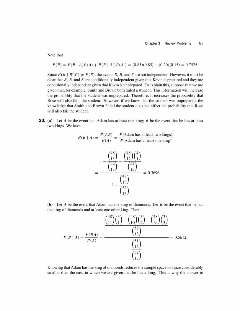
Chapter 3 Review Problems 61
Note that
P(R) = P(R | A)P (A) + P(R | Ac)P (Ac) = (0.85)(0.85) + (0.20)(0.15) = 0.7525.
Since P(R | BcSc) �= P(R), the events R, B, and S are not independent. However, it must beclear that R, B, and S are conditionally independent given that Kevin is prepared and they areconditionally independent given that Kevin is unprepared. To explain this, suppose that we aregiven that, for example, Smith and Brown both failed a student. This information will increasethe probability that the student was unprepared. Therefore, it increases the probability thatRose will also fails the student. However, if we know that the student was unprepared, theknowledge that Smith and Brown failed the student does not affect the probability that Rosewill also fail the student.
20. (a) Let A be the event that Adam has at least one king; B be the event that he has at leasttwo kings. We have
P(B | A) = P(AB)
P (A)= P(Adam has at least two kings)
P (Adam has at least one king)
=
1 −
(48
13
)(
52
13
) −
(48
12
)(4
1
)(
52
13
)
1 −
(48
13
)(
52
13
)= 0.3696.
(b) Let A be the event that Adam has the king of diamonds. Let B be the event that he hasthe king of diamonds and at least one other king. Then
P(B | A) = P(BA)
P (A)=
(48
11
)(3
1
)+(
48
10
)(3
2
)+(
48
9
)(3
3
)(
52
13
)(
51
12
)(
52
13
)= 0.5612.
Knowing that Adam has the king of diamonds reduces the sample space to a size considerablysmaller than the case in which we are given that he has a king. This is why the answer to

62 Chapter 3 Conditional Probability and Independence
part (b) is larger than the answer to part (a). If one is not convinced of this, he or she shouldsolve the problem in a simpler case. For example, a case in which there are four cards, say,king of diamonds, king of hearts, jack of clubs, and eight of spade. If two cards are drawn,the reduced sample space in the case Adam announces that he has a king is
{KdKh, KdJc, Kd8s, KhJc, Kh8s},while the reduced sample space in the case Adam announces that he has the king of diamondsis
{KdKh, KdJc, Kd8s}.In the first case, the probability of more kings is 1/5; in the second case the probability ofmore kings is 1/3.

Chapter 4
Distribution Functions and
Discrete Random Variables
4.2 DISTRIBUTION FUNCTIONS
1. The set of possible values of X is {0, 1, 2, 3, 4, 5}. The probabilities associated with thesevalues are
x 0 1 2 3 4 5P(X = x) 6/36 10/36 8/36 6/36 4/36 2/36
2. The set of possible values of X is {−6, −2, −1, 2, 3, 4}. The probabilities associated withthese values are
P(X = −6) = P(X = 2) = P(X = 4) =
(5
2
)(
15
2
) = 0.095,
P (X = −2) = P(X = −1) = P(X = 3) =
(5
1
)(5
1
)(
15
2
) = 0.238.
3. The set of possible values of X is {0, 1, 2 . . . , N}. Assuming that people have the diseaseindependent of each other,
P(X = i) ={
(1 − p)i−1p 1 ≤ i ≤ N
(1 − p)N i = 0.
4. Let X be the length of the side of a randomly chosen plastic die manufactured by the factory,then
P(X3 > 1.424) = P(X > 1.125) = 1.25 − 1.125
1.25 − 1= 1
2.

64 Chapter 4 Distribution Functions and Discrete Random Variables
5. P(X < 1) = F(1−) = 1/2.
P (X = 1) = F(1) − F(1−) = 1/6.
P (1 ≤ X < 2) = F(2−) − F(1−) = 1/4.
P (X > 1/2) = 1 − F(1/2) = 1 − 1/2 = 1/2.
P (X = 3/2) = 0.
P (1 < X ≤ 6) = F(6) − F(1) = 1 − 2/3 = 1/3.
6. Let F be the distribution function of X. Then
F(t) =
⎧⎪⎪⎪⎪⎪⎪⎪⎪⎨⎪⎪⎪⎪⎪⎪⎪⎪⎩
0 t < 0
1/8 0 ≤ t < 1
1/2 1 ≤ t < 2
7/8 2 ≤ t < 3
1 t ≥ 3.
7. Note that X is neither continuous nor discrete. The answers are
(a) F(6−) = 1 implies that k(−36 + 72 − 3) = 1; so k = 1/33.
(b) F(4) − F(2) = 29/33 − 4/33 = 25/33.
(c) 1 − F(3) = 1 − (24/33) = 9/33.
(d) P(X ≤ 4 | X ≥ 3) = F(4) − F(3−)
1 − F(3−)=
29
33− 9
33
1 − 9
33
= 5
6.
8. F(Q0.5) = 1/2 implies that 1 + e−x = 2. The only solution of this question is x = 0. Sox = 0 is the median of F . Similarly, F(Q0.25) = 1/4 implies that 1 + e−x = 4, the solutionof which is x = − ln 3. F (Q0.75) = 3/4 implies that 1 + e−x = 4/3, the solution of which isx = ln 3. So − ln 3 and ln 3 are the first and the third quartiles of F , respectively. Therefore,50% of the years the rate at which the price of oil per gallon changes is negative or zero, 25%of the years the rate is − ln 3 ≈ −1.0986 or less, and 75% of the years the rate is ln 3 ≈ 1.0986or less.
9. (a)
P(|X| ≤ t) = P(−t ≤ X ≤ t) = P(X ≤ t) − P(X < −t)
= F(t) − [1 − P(X ≥ −t)
] = F(t) − [1 − P(x ≤ t)
] = 2F(t) − 1.
(b) Using part (a), we have
P(|X| > t) = 1 − P(|X| ≤ t) = 1 − [2F(t) − 1
] = 2[1 − F(t)
].

Section 4.2 Distribution Functions 65
(c)
P(X = t) = 1 + P(X = t) − 1 = P(X ≤ t) + P(X > t) + P(X = t) − 1
= P(X ≤ t) + P(X ≥ t) − 1 = P(X ≤ t) + P(X ≤ −t) − 1
= F(t) + F(−t) − 1.
10. F is a distribution function because F(−∞) = 0, F(∞) = 1, F is right continuous, and
F ′(t) = 1
πe−t > 0 implies that F is nondecreasing.
11. F is a distribution function because F(−∞) = 0, F(∞) = 1, F is right continuous, and
F ′(t) = 1
(1 + t)2> 0 implies that it is nondecreasing.
12. Clearly, F is right continuous. On t < 0 and on t ≥ 0, it is increasing, limt→∞ F(t) = 1,and limt→−∞ F(t) = 0. It looks like F satisfies all of the conditions necessary to makeit a distribution function. However, F(0−) = 1/2 > F(0+) = 1/4 shows that F is notnondecreasing. Therefore, F is not a probability distribution function.
13. Let the departure time of the last flight before the passenger arrives be 0. Then Y , the arrivaltime of the passenger is a random number from (0, 45). The waiting time is X = 45 − Y . Wehave that for 0 ≤ t ≤ 45,
P(X ≤ t) = P(45 − Y ≤ t) = P(Y ≥ 45 − t) = 45 − (45 − t)
45= t
45.
So F , the distribution function of X is
F(t) =
⎧⎪⎪⎨⎪⎪⎩0 t < 0
t/45 0 ≤ t < 45
1 t ≥ 45.
14. Let X be the first two-digit number selected from the set {00, 01, 02, . . . , 99} which is between4 and 18. Since for i = 4, 5, . . . , 18,
P (X = i | 4 ≤ X ≤ 18) = P(X = i)
P (4 ≤ X ≤ 18)= 1/100
15/100= 1
15,
we have that X is chosen randomly from the set {4, 5, . . . , 18}.15. Let X be the minimum of the three numbers,
P(X < 5) = 1 − P(X ≥ 5) = 1 −
(36
3
)(
40
3
) = 0.277.

66 Chapter 4 Distribution Functions and Discrete Random Variables
16.
P(X2 −5X+6 > 0) = P((X−2)(X−3) > 0
) = P(X < 2)+P(X > 3) = 2 − 0
3 − 0+0 = 2
3.
17.
F(t) =
⎧⎪⎪⎪⎪⎨⎪⎪⎪⎪⎩0 t < 0
t
1 − t0 ≤ t < 1/2
1 t ≥ 1/2.
18. The distribution function of X is F(t) = 0 if t < 1; F(t) = 1 − (89/90)n if n ≤ t < n + 1,n ≥ 1. Since
F(26−) = 1 −(89
90
)25 = 0.244 < 0.25 < 1 −(89
90
)26 = 0.252 = F(26),
26 is the first quartile. Since
F(63−) = 1 −(89
90
)62 = 0.4998 < 0.5 < 1 −(89
90
)63 = 0.505 = F(63),
63 is the median of X. Similarly,
F(125−) = 1 −(89
90
)124 = 0.7498 < 0.75 < 1 −(89
90
)125 = 0.753 = F(125),
implies that 125 is the third quartile of X.
19.
G(t) =⎧⎨⎩F(t) t < 5
1 t ≥ 5.
4.3 DISCRETE RANDOM VARIABLES
1. F , the distribution functions of X is given by
F(x) =
⎧⎪⎪⎪⎪⎪⎪⎪⎪⎪⎪⎪⎨⎪⎪⎪⎪⎪⎪⎪⎪⎪⎪⎪⎩
0 if x < 1
1/15 if 1 ≤ x < 2
3/15 if 2 ≤ x < 3
6/15 if 3 ≤ x < 4
10/15 if 4 ≤ x < 5
1 if x ≥ 5.

Section 4.3 Discrete Random Variables 67
2. p, the probability mass function of X, is given by
x 1 2 3 4 5 6p(x) 11/36 9/36 7/36 5/36 3/36 1/36
F , the probability distribution function of X, is given by
F(x) =
⎧⎪⎪⎪⎪⎪⎪⎪⎪⎪⎪⎪⎪⎪⎪⎨⎪⎪⎪⎪⎪⎪⎪⎪⎪⎪⎪⎪⎪⎪⎩
0 if x < 1
11/36 if 1 ≤ x < 2
20/36 if 2 ≤ x < 3
27/36 if 3 ≤ x < 4
32/36 if 4 ≤ x < 5
35/36 if 5 ≤ x < 6
1 if x ≥ 6.
3. The possible values of X are 2, 3, . . . , 12. The sample space of this experiment consists of 36equally likely outcomes. Hence the probability of any of them is 1/36. Thus
p(2) = P(X = 2) = P({
(1, 1)}) = 1/36,
p(3) = P(X = 3) = P({
(1, 2), (2, 1)}) = 2/36,
p(4) = P(X = 4) = P({
(1, 3), (2, 2), (3, 1)}) = 3/36.
Similarly,
i 5 6 7 8 9 10 11 12p(i) 4/36 5/36 6/36 5/36 4/36 3/36 2/36 1/36
4. Let p be the probability mass function of X. We have
x −2 2 4 6p(x) 1/2 1/10 13/45 1/9
5. Let p be the probability mass function of X and q be the probability mass function of Y . Wehave
p(i) =( 9
10
)i−1( 1
10
), i = 1, 2, . . . .
q(j) = P(Y = j) = P(X = j − 1
2
)=( 9
10
)(j−3)/2( 1
10
), j = 3, 5, 7, . . . .
6. Mode of p = 1; mode of q = 1.

68 Chapter 4 Distribution Functions and Discrete Random Variables
7. (a)∑5
k=1 kx = 1 ⇒ k = 1/15.
(b) k(−1)2 + k + 4k + 9k = 1 ⇒ k = 1/15.
(c)∞∑
x=1
k(1
9
)x = 1 ⇒ k = 1∑∞x=1(1/9)x
= 1/[ 1/9
1 − (1/9)
]= 8.
(d) k(1 + 2 + · · · + n) = 1 ⇒ k = 1[n(n + 1)
]/2
= 2
n(n + 1).
(e) k(12 + 22 + · · · + n2) = 1 ⇒ k = 6
n(n + 1)(2n + 1).
8. Let p be the probability mass function of X; then
p(i) = P(X = i) =
(18
i
)(28
12 − i
)(
46
12
) i = 0, 1, 2, . . . , 12.
9. For x < 0, F(x) = 0. If x ≥ 0, for some nonnegative integer n, n ≤ x < n + 1, and we havethat
F(x) =n∑
i=0
3
4
(1
4
)i = 3
4
[1 +
(1
4
)+(1
4
)2 + · · · +(1
4
)n]
= 3
4· 1 − (1/4)n+1
1 − (1/4)= 1 −
(1
4
)n+1.
Thus
F(x) ={
0 if x < 0
1 − (1/4)n+1 if n ≤ x < n + 1, n = 0, 1, 2, . . . .
10. Let p be the probability mass function of X and F be its distribution function. We have
p(i) =(5
6
)i−1(1
6
), i = 1, 2, 3, . . . .
F (x) = 0 for x < 1. If x ≥ 1, for some positive integer n, n ≤ x < n + 1, and we have that
F(x) =n∑
i=1
(5
6
)i−1(1
6
)= 1
6
[1 +
(5
6
)+(5
6
)2 + · · · +(5
6
)n−1]= 1
6· 1 − (5/6)n
1 − (5/6)= 1 −
(5
6
)n
.

Section 4.3 Discrete Random Variables 69
Hence
F(x) =
⎧⎪⎨⎪⎩0 if x < 1
1 −(5
6
)n
if n ≤ x < n + 1, n = 1, 2, 3, . . . .
11. The set of possible values of X is {2, 3, 4, . . . }. For n ≥ 2, X = n if and only if either all ofthe first n − 1 bits generated are 0 and the nth bit generated is 1, or all of the first n − 1 bitsgenerated are 1 and the nth bit generated is 0. Therefore, by independence,
P(X = n) =(1
2
)n−1 · 1
2+(1
2
)n−1 · 1
2=(1
2
)n−1, n ≥ 2.
12. The event Z > i occurs if and only if Liz has not played with Bob since i Sundays ago, andthe earliest she will play with him is next Sunday. Now the probability is i/k that Liz willplay with Bob if last time they played was i Sundays ago; hence
P(Z > i) = 1 − i
k, i = 1, 2, . . . , k − 1.
Let p be the probability mass function of Z. Then, using this fact for 1 ≤ i ≤ k, we obtain
p(i) = P(Z = i) = P(Z > i − 1) − P(Z > i) =(
1 − i − 1
k
)−(
1 − i
k
)= 1
k.
13. The possible values of X are 0, 1, 2, 3, 4, and 5. For i, 0 ≤ i ≤ 5,
P(X = i) =
(5
i
)6Pi · 9P5−i · 10!
15! .
The numerical values of these probabilities are as follows.
i 0 1 2 3 4 5P(X = i) 42/1001 252/1001 420/1001 240/1001 45/1001 2/1001
14. For i = 0, 1, 2, and 3, we have
P(X = i) =
(10
i
)(10 − i
6 − 2i
)26−2i(
20
6
) .
The numerical values of these probabilities are as follows.
i 0 1 2 3p(i) 112/323 168/323 42/323 1/323
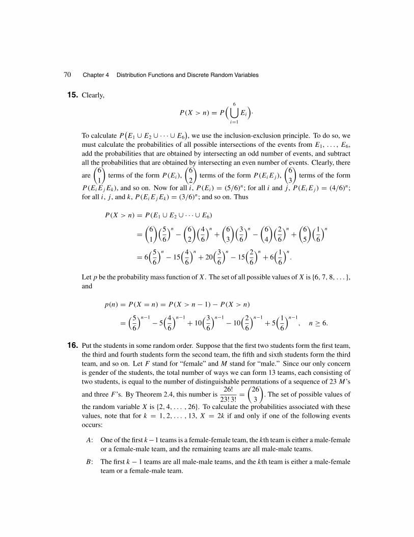
70 Chapter 4 Distribution Functions and Discrete Random Variables
15. Clearly,
P(X > n) = P( 6⋃
i=1
Ei
)·
To calculate P(E1 ∪ E2 ∪ · · · ∪ E6
), we use the inclusion-exclusion principle. To do so, we
must calculate the probabilities of all possible intersections of the events from E1, . . . , E6,add the probabilities that are obtained by intersecting an odd number of events, and subtractall the probabilities that are obtained by intersecting an even number of events. Clearly, there
are
(6
1
)terms of the form P(Ei),
(6
2
)terms of the form P(EiEj ),
(6
3
)terms of the form
P(EiEjEk), and so on. Now for all i, P(Ei) = (5/6)n; for all i and j , P(EiEj ) = (4/6)n;for all i, j , and k, P(EiEjEk) = (3/6)n; and so on. Thus
P(X > n) = P(E1 ∪ E2 ∪ · · · ∪ E6)
=(
6
1
)(5
6
)n −(
6
2
)(4
6
)n +(
6
3
)(3
6
)n −(
6
4
)(2
6
)n +(
6
5
)(1
6
)n
= 6(5
6
)n − 15(4
6
)n + 20(3
6
)n − 15(2
6
)n + 6(1
6
)n
.
Let p be the probability mass function of X. The set of all possible values of X is {6, 7, 8, . . . },and
p(n) = P(X = n) = P(X > n − 1) − P(X > n)
=(5
6
)n−1 − 5(4
6
)n−1 + 10(3
6
)n−1 − 10(2
6
)n−1 + 5(1
6
)n−1, n ≥ 6.
16. Put the students in some random order. Suppose that the first two students form the first team,the third and fourth students form the second team, the fifth and sixth students form the thirdteam, and so on. Let F stand for “female” and M stand for “male.” Since our only concernis gender of the students, the total number of ways we can form 13 teams, each consisting oftwo students, is equal to the number of distinguishable permutations of a sequence of 23 M’s
and three F ’s. By Theorem 2.4, this number is26!
23! 3! =(
26
3
). The set of possible values of
the random variable X is {2, 4, . . . , 26}. To calculate the probabilities associated with thesevalues, note that for k = 1, 2, . . . , 13, X = 2k if and only if one of the following eventsoccurs:
A: One of the first k−1 teams is a female-female team, the kth team is either a male-femaleor a female-male team, and the remaining teams are all male-male teams.
B: The first k − 1 teams are all male-male teams, and the kth team is either a male-femaleteam or a female-male team.

Section 4.4 Expectations of Discrete Random Variables 71
To find P(A), note that for A to occur, there are k−1 possibilities for one of the first k−1 teamsto be a female-female team, two possibilities for the kth team (male-female and female-male),and one possibility for the remaining teams to be all male-male teams. Therefore,
P(A) = 2(k − 1)(26
3
) .
To find P(B), note that for B to occur, there is one possibility for the first k − 1 teams tobe all male-male, and two possibilities for the kth team: male-female and female-male. Thenumber of possibilities for the remaining 13−k teams is equal to the number of distinguishable
permutations of two F ’s and (26−2k)−2 M’s, which, by Theorem 2.4, is26 − 2k)!
2! (26 − 2k − 2)! =(26 − 2k
2
). Therefore,
P(B) =2
(26 − 2k
2
)(
26
3
) .
Hence, for 1 ≤ k ≤ 13,
P (X = 2k) = P(A) + P(B) =2(k − 1) + 2
(26 − 2k
2
)(
26
3
) = 1
650k2 − 1
26k + 1
4.
4.4 EXPECTATIONS OF DISCRETE RANDOM VARIABLES
1. Yes, of course there is a fallacy in Dickens’ argument. If, in England, at that time there wereexactly two train accidents each month, then Dickens would have been right. Usually, for alln > 0 and for any two given days, the probability of n train accidents in day 1 is equal to theprobability of n accidents in day 2. Therefore, in all likelihood the risk of train accidents onthe final day in March and the risk of such accidents on the first day in April would have beenabout the same. The fact that train accidents occurred at random days, two per month on theaverage, imply that in some months more than two and in other months two or less accidentswere occurring.
2. Let X be the fine that the citizen pays on a random day. Then
E(X) = 25(0.60) + 0(0.40) = 15.
Therefore, it is much better to park legally.

72 Chapter 4 Distribution Functions and Discrete Random Variables
3. The expected value of the winning amount is
30( 4000
2, 000, 000
)+ 800
( 500
2, 000, 000
)+ 1, 200, 000
( 1
2, 000, 000
)= 0.86.
Considering the cost of the ticket, the expected value of the player’s gain in one game is−1 + 0.86 = −0.14.
4. Let X be the amount that the player gains in one game, then
P(X = 4) =
(4
3
)(6
1
)(
10
4
) = 0.114, P (X = 9) = 1(10
4
) = 0.005,
and P(X = −1) = 1 − 0.114 − 0.005 = 0.881. Thus
E(X) = −1(0.881) + 4(0.114) + 9(0.005) = −0.38.
Therefore, on the average, the player loses 38 cents per game.
5. LetX be the net gain in one play of the game. The set of possible values ofX is {−8, −4, 0, 6, 10}.The probabilities associated with these values are
p(−8) = p(0) = 1(5
2
) = 1
10, p(−4) =
(2
1
)(2
1
)(
5
2
) = 4
10,
and p(6) = p(10) =
(2
1
)(
5
2
) = 2
10. Hence
E(X) = −8 · 1
10− 4 · 4
10+ 0 · 1
10+ 6 · 2
10+ 10 · 2
10= 4
5.
Since E(X) > 0, the game is not fair.
6. The expected number of defective items is
3∑i=0
i ·
(5
i
)(15
5 − i
)(
20
3
) = 0.75.

Section 4.4 Expectations of Discrete Random Variables 73
7. For i = 4, 5, 6, 7, let Xi be the profit if i magazines are ordered. Then
E(X4) = 4a
3,
E(X5) = 2a
3· 6
18+ 5a
3· 12
18= 4a
3,
E(X6) = 0 · 6
18+ a · 5
18+ 6a
3· 7
18= 19a
18,
E(X7) = −2a
3· 6
18+ a
3· 5
18+ 4a
3· 4
18+ 7a
3· 3
18= 10a
18.
Since 4a/3 > 19a/18 and 4a/3 > 10a/18, either 4, or 5 magazines should be ordered tomaximize the profit in the long run.
8. (a)∞∑
x=1
6
π2x2= 6
π2
∞∑x=1
1
x2= 6
π2· π2
6= 1.
(b) E(X) =∞∑
x=1
x6
π2x2= 6
π2
∞∑x=1
1
x= ∞.
9. (a)2∑
i=−2
p(x) = 9
27+ 4
27+ 1
27+ 4
27+ 9
27= 1.
(b) E(X) = ∑2x=−2 xp(x) = 0, E(|X|) = ∑2
x=−2 |x|p(x) = 44/27,
E(X2) = ∑2x=−2 x2p(x) = 80/27. Hence
E(2X2 − 5X + 7) = 2(80/27) − 5(0) + 7 = 349/27.
10. Let R be the radius of the randomly selected disk; then E(2πR) = 2π
10∑i=1
i1
10= 11π.
11. p(x) the probability mass function of X is given by
x −3 0 3 4p(x) 3/8 1/8 1/4 1/4
Hence
E(X) = −3 · 3
8+ 0 · 1
8+ 3 · 1
4+ 4 · 1
4= 5
8,
E(X2) = 9 · 3
8+ 0 · 1
8+ 9 · 1
4+ 16 · 1
4= 77
8,

74 Chapter 4 Distribution Functions and Discrete Random Variables
E(|X|) = 3 · 3
8+ 0 · 1
8+ 3 · 1
4+ 4 · 1
4= 23
8,
E(X2 − 2|X|) = 77
8− 2
(23
8
)= 31
8,
E(X|X|) = −9 · 3
8+ 0 · 1
8+ 9 · 1
4+ 16 · 1
4= 23
8.
12. E(X) =10∑i=1
i · 1
10= 11
2and E(X2) =
10∑i=1
i2 · 1
10= 77
2. So
E[X(11 − X)
] = E(11X − X2) = 11 · 11
2− 77
2= 22.
13. Let X be the number of different birthdays; we have
P(X = 4) = 365 × 364 × 363 × 362
3654= 0.9836,
P (X = 3) =
(4
2
)365 × 364 × 363
3654= 0.0163,
P (X = 2) =
(4
2
)365 × 364 +
(4
3
)365 × 364
3654= 0.00007,
P (X = 1) = 365
3654= 0.000000021.
Thus
E(X) = 4(0.9836) + 3(0.0163) + 2(0.00007) + 1(0.000, 000, 021) = 3.98.
14. Let X be the number of children they should continue to have until they have one of each sex.For i ≥ 2, clearly, X = i if and only if either all of their first i −1 children are boys and the ithchild is a girl, or all of their first i − 1 children are girls and the ith child is a boy. Therefore,by independence,
P(X = i) =(1
2
)i−1 · 1
2+(1
2
)i−1 · 1
2=(1
2
)i−1, i ≥ 2.
So
E(X) =∞∑i=2
i(1
2
)i−1 = −1 +∞∑i=1
i(1
2
)i−1 = −1 + 1
(1 − 1/2)2= 3.
Note that for |r| < 1,∑∞
i=1 iri−1 = 1/[(1 − r)2].

Section 4.4 Expectations of Discrete Random Variables 75
15. Let Aj be the event that the person belongs to a family with j children. Then
P(K = k) =c∑
j=0
P(K = k|Aj)P (Aj) =c∑
j=k
1
jαj .
Therefore,
E(K) =c∑
k=1
kP (K = k) =c∑
k=1
k
c∑j=k
αj
j=
c∑k=1
c∑j=k
kαj
j.
16. Let X be the number of cards to be turned face up until an ace appears. Let A be the eventthat no ace appears among the first i − 1 cards that are turned face up. Let B be the event thatthe ith card turned face up is an ace. We have
P(X = i) = P(AB) = P(B|A)P (A) = 4
52 − (i − 1)·
(48
i − 1
)(
52
i − 1
) .
Therefore,
E(X) =49∑i=1
i
(48
i − 1
)4(
52
i − 1
)(53 − i)
= 10.6.
To some, this answer might be counterintuitive.
17. Let X be the largest number selected. Clearly,
P(X = i) = P(X ≤ i) − P(X ≤ i − 1) =( i
N
)n −( i − 1
N
)n
, i = 1, 2, . . . , N.
Hence
E(X) =N∑
i=1
[ i n+1
Nn− i(i − 1)n
Nn
]= 1
Nn
N∑i=1
[i n+1 − i(i − 1)n
]
= 1
Nn
N∑i=1
[i n+1 − (i − 1)n+1 − (i − 1)n
] =Nn+1 −
N∑i=1
(i − 1)n
Nn.
For large N ,N∑
i=1
(i − 1)n ≈∫ N
0xn dx = Nn+1
n + 1.

76 Chapter 4 Distribution Functions and Discrete Random Variables
Therefore,
E(X) ≈Nn+1 − Nn+1
n + 1Nn
= nN
n + 1.
18. (a) Note that1
n(n + 1)= 1
n− 1
n + 1.
Sok∑
n=1
1
n(n + 1)=
k∑n=1
(1
n− 1
n + 1
)= 1 − 1
k + 1.
This implies that
∞∑n=1
p(n) = limk→∞
k∑n=1
1
n(n + 1)= 1 − lim
k→∞1
k + 1= 1.
Therefore, p is a probability mass function.
(b) E(X) =∞∑
n=1
np(n) =∞∑
n=1
1
n + 1= ∞,
where the last equality follows since we know from calculus that the harmonic series,1 + 1/2 + 1/3 + · · · , is divergent. Hence E(X) does not exist.
19. By the solution to Exercise 16, Section 4.3, it should be clear that for 1 ≤ k ≤ n,
P(X = 2k) =2(k − 1) + 2
(2n − 2k
2
)(
2n
3
) .
Hence
E(X) =n∑
k=1
2kP (X = 2k) =n∑
k=1
=4k(k − 1) + 4k
(2n − 2k
2
)(
2n
3
)
= 4(2n
3
)[2 n∑k=1
k3 − (4n − 2)
n∑k=1
k2 + (2n2 − n − 1)
n∑n=1
k]
= 4(2n
3
)[2 · n2 (n + 1)2
4− (4n − 2) · n(n + 1)(2n + 1)
6+ (2n2 − n − 1)
n(n + 1)
2
]
= (n + 1)2
2n − 1.

Section 4.5 Variances and Moments of Discrete Random Variables 77
4.5 VARIANCES AND MOMENTS OF DISCRETE RANDOM VARIABLES
1. On average, in the long run, the two businesses have the same profit. The one that has a profitwith lower standard deviation should be chosen by Mr. Jones because he’s interested in steadyincome. Therefore, he should choose the first business.
2. The one with lower standard deviation, namely, the second device.
3. E(X) = ∑3x=−3 xp(x) = −1, E(X2) = ∑3
x=−3 x2p(x) = 4.Therefore, Var(X) = 4−1 = 3.
4. p, the probability mass function of X is given by
x −3 0 6p(x) 3/8 3/8 2/8
Thus
E(X) = −9
8+ 12
8= 3
8, E(X2) = 27
8+ 72
8= 99
8,
Var(X) = 99
8− 9
64= 783
64= 12.234, σX = √
12.234 = 3.498.
5. By straightforward calculations,
E(X) =N∑
i=1
i · 1
N= 1
N· N(N + 1)
2= N + 1
2,
E(X2) =N∑
i=1
i2 · 1
N= 1
N· N(N + 1)(2N + 1)
6= (N + 1)(2N + 1)
6,
Var(X) = (N + 1)(2N + 1)
6− (N + 1)2
4= N2 − 1
12,
σX =√
N2 − 1
12.
6. Clearly,
E(X) =5∑
i=0
i ·
(13
i
)(39
5 − i
)(
52
5
) = 1.25,
E(X2) =5∑
i=0
i2 ·
(13
i
)(39
5 − i
)(
52
5
) = 2.426.

78 Chapter 4 Distribution Functions and Discrete Random Variables
Therefore, Var(X) = 2.426 − (1.25)2 = 0.864, and hence σX = √0.864 = 0.9295.
7. By the Corollary of Theorem 4.2, E(X2 − 2X) = 3 implies that E(X2) − 2E(X) = 3.
Substituting E(X) = 1 in this relation gives E(X2) = 5. Hence, by Theorem 4.3,
Var(X) = E(X2) − [E(X)
]2 = 5 − 1 = 4.
By Theorem 4.5,Var(−3X + 5) = 9Var(X) = 9 × 4 = 36.
8. Let X be Harry’s net gain. Then
X =
⎧⎪⎪⎪⎪⎨⎪⎪⎪⎪⎩−2 with probability 1/8
0.25 with probability 3/8
0.50 with probability 3/8
0.75 with probability 1/8.
Thus
E(X) = −2 · 1
8+ 0.25 · 3
8+ 0.50 · 3
8+ 0.75 · 1
8= 0.125
E(X2) = (−2)2 · 1
8+ 0.252 · 3
8+ 0.502 · 3
8+ 0.752 · 1
8= 0.6875.
These show that the expected value of Harry’s net gain is 12.5 cents. Its variance is
Var(X) = 0.6875 − 0.1252 = 0.671875.
9. Note that E(X) = E(Y ) = 0. Clearly,
P(|X − 0| ≤ t
) ={
0 if t < 1
1 if t ≥ 1,
P(|Y − 0| ≤ t
) ={
0 if t < 10
1 if t ≥ 10.
These relations, clearly, show that for all t > 0,
P(|Y − 0| ≤ t
) ≤ P(|X − 0| ≤ t
).
Therefore, X is more concentrated about 0 than Y is.
10. (a) Let X be the number of trials required to open the door. Clearly,
P(X = x) =(
1 − 1
n
)x−1 1
n, x = 1, 2, 3, . . . .

Section 4.5 Variances and Moments of Discrete Random Variables 79
Thus
E(X) =∞∑
x=1
x(
1 − 1
n
)x−1 1
n= 1
n
∞∑x=1
x(
1 − 1
n
)x−1. (10)
We know from calculus that ∀r , |r| < 1,
∞∑x=1
xrx−1 = 1
(1 − r)2. (11)
Thus
∞∑x=1
x(
1 − 1
n
)x−1 = 1[1 −
(1 − 1
n
)]2= n2. (12)
Substituting (12) in (10), we obtain E(X) = n. To calculate Var(X), first we find E(X2). Wehave
E(X2) =∞∑
x=1
x2(
1 − 1
n
)x−1(1
n
)= 1
n
∞∑x=1
x2(
1 − 1
n
)x−1. (13)
Now to calculate this sum, we multiply both sides of (11) by r and then differentiate it withrespect to r; we get
∞∑x=1
x2rx−1 = 1 + r
(1 − r)3.
Using this relation in (13), we obtain
E(X2) = 1
n·
1 + 1 − 1
n[1 −
(1 − 1
n
)]3= 2n2 − n.
Therefore,
Var(X) = (2n2 − n) − n2 = n(n − 1).
(b) Let Ai be the event that on the ith trial the door opens. Let X be the number of trialsrequired to open the door. Then
P(X = 1) = 1
n,

80 Chapter 4 Distribution Functions and Discrete Random Variables
P(X = 2) = P(Ac1A2) = P(A2|Ac
1)P (Ac1)
= 1
n − 1· n − 1
n= 1
n,
P (X = 3) = P(Ac1A
c2A3) = P(A3|Ac
2Ac1)P (Ac
2Ac1)
= P(A3|Ac2A
c1)P (Ac
2|Ac1)P (Ac
1)
= 1
n − 2· n − 2
n − 1· n − 1
n= 1
n.
Similarly, P(X = i) = 1/n for 1 ≤ i ≤ n. Therefore, X is a random number selected from{1, 2, 3, . . . , n}. By Exercise 5, E(X) = (n + 1)/2 and Var(X) = (n2 − 1)/12.
11. For E(X3) to exist, we must have E(|X3|) < ∞. Now
∞∑n=1
x3n p(xn) = 6
π2
∞∑n=1
(−1)nn√
n
n2= 6
π2
∞∑n=1
(−1)n
√n
< ∞,
whereas
E(|X3|) =
∞∑n=1
|x3n|p(xn) = 6
π2
∞∑n=1
n√
n
n2= 6
π2
∞∑n=1
1√n
= ∞.
12. For 0 < s < r , clearly,
|x|s ≤ max(1, |x|r) ≤ 1 + |x|r , ∀x ∈ R .
Let A be the set of possible values of X and p be its probability mass function. Since the rthabsolute moment of X exists,
∑x∈A |x|rp(x) < ∞. Now∑
x∈A
|x|sp(x) ≤∑x∈A
(1 + |x|r)p(x)
=∑x∈A
p(x) +∑x∈A
|x|rp(x) = 1 +∑x∈A
|x|rp(x) < ∞,
implies that the absolute moment of order s of X also exists.
13. Var(X)=Var(Y ) implies that
E(X2) − [E(X)
]2 = E(Y 2) − [E(Y )
]2.
Since E(X) = E(Y ), this implies that E(X2) = E(Y 2). Let
P(X = a) = p1, P (X = b) = p2, P (X = c) = p3;P(Y = a) = q1, P (Y = b) = q2, P (Y = c) = q3.

Section 4.5 Variances and Moments of Discrete Random Variables 81
Clearly,
p1 + p2 + p3 = q1 + q2 + q3 = 1.
This implies
(p1 − q1) + (p2 − q2) + (p3 − q3) = 0. (14)
The relations E(X) = E(Y ) and E(X2) = E(Y 2) imply that
ap1 + bp2 + cp3 = aq1 + bq2 + cq3
a2p1 + b2p2 + c2p3 = a2q1 + b2q2 + c2q3.
These and equation (14) give us the following system of 3 equations in the 3 unknowns p1 −q1,p2 − q2, and p3 − q3.⎧⎪⎨⎪⎩
(p1 − q1) + (p2 − q2) + (p3 − q3) = 0
a(p1 − q1) + b(p2 − q2) + c(p3 − q3) = 0
a2(p1 − q1) + b2(p2 − q2) + c2(p3 − q3) = 0.
In matrix form, this is equivalent to⎛⎝ 1 1 1a b c
a2 b2 c2
⎞⎠⎛⎝p1 − q1
p2 − q2
p3 − q3
⎞⎠ =⎛⎝0
00
⎞⎠ . (15)
Now
det
⎛⎝ 1 1 1a b c
a2 b2 c2
⎞⎠ = bc2 + ca2 + ab2 − ba2 − cb2 − ac2
= (c − a)(c − b)(b − a) �= 0,
since a, b, and c are three different real numbers. This implies that the matrix⎛⎝ 1 1 1a b c
a2 b2 c2
⎞⎠is invertible. Hence the solution to (15) is
p1 − q1 = p2 − q2 = p3 − q3 = 0.
Therefore, p1 = q1, p2 = q2, p3 = q3 implying that X and Y are identically distributed.

82 Chapter 4 Distribution Functions and Discrete Random Variables
14. Let
P(X = a1) = p1, P (X = a2) = p2, . . . , P (X = an) = pn;P(Y = a1) = q1, P (Y = a2) = q2, . . . , P (Y = an) = qn.
Clearly,p1 + p2 + · · · + pn = q1 + q2 + · · · + qn = 1.
This implies that(p1 − q1) + (p2 − q2) + · · · + (pn − qn) = 0.
The relations E(Xr) = E(Y r), for r = 1, 2, . . . , n − 1 imply that
a1p1 + a2p2 + · · · + anpn = a1q1 + a2q2 + · · · + anqn,
a21p1 + a2
2p2 + · · · + a2npn = a2
1q1 + a22q2 + · · · + a2
nqn,
...
an−11 p1 + an−1
2 p2 + · · · + an−1n pn = an−1
1 q1 + an−12 q2 + · · · + an−1
n qn.
These and the previous relation give us the following n equations in the n unknowns p1 − q1,p2 − q2, . . . , pn − qn.⎧⎪⎪⎪⎪⎪⎪⎨⎪⎪⎪⎪⎪⎪⎩
(p1 − q1) + (p2 − q2) + · · · + (pn − qn) = 0
a1(p1 − q1) + a2(p2 − q2) + · · · + an(pn − qn) = 0
a21(p1 − q1) + a2
2(p2 − q2) + · · · + a2n(pn − qn) = 0
. . . . . . . . . . . . . . . . . . . . . . . . . . . . . . . . . . . . . . . . . . . . . . . . . . . . . .an−1
1 (p1 − q1) + an−12 (p2 − q2) + · · · + an−1
n (pn − qn) = 0
In matrix form, this is equivalent to⎛⎜⎜⎜⎜⎜⎝1 1 · · · 1a1 a2 · · · an
a21 a2
2 · · · a2n
......
...
an−11 an−1
2 · · · an−1n
⎞⎟⎟⎟⎟⎟⎠
⎛⎜⎜⎜⎜⎜⎝p1 − q1
p2 − q2
p3 − q3...
pn − qn
⎞⎟⎟⎟⎟⎟⎠ =
⎛⎜⎜⎜⎜⎜⎝000...
0
⎞⎟⎟⎟⎟⎟⎠ . (16)
Now
det
⎛⎜⎜⎜⎜⎜⎝1 1 · · · 1a1 a2 · · · an
a21 a2
2 · · · a2n
......
...
an−11 an−1
2 · · · an−1n
⎞⎟⎟⎟⎟⎟⎠ =∏
j=n,n−1,... ,2i<j
(aj − ai) �= 0,
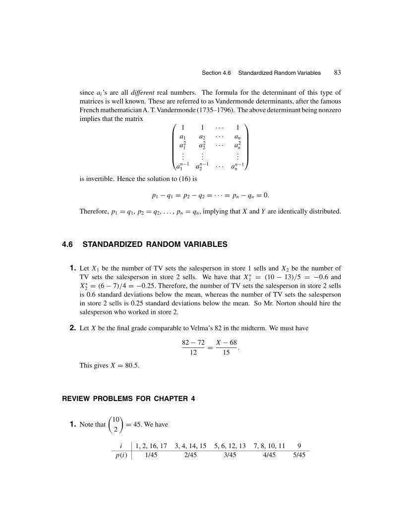
Section 4.6 Standardized Random Variables 83
since ai’s are all different real numbers. The formula for the determinant of this type ofmatrices is well known. These are referred to as Vandermonde determinants, after the famousFrench mathematicianA. T.Vandermonde (1735–1796). The above determinant being nonzeroimplies that the matrix ⎛⎜⎜⎜⎜⎜⎝
1 1 · · · 1a1 a2 · · · an
a21 a2
2 · · · a2n
......
...
an−11 an−1
2 · · · an−1n
⎞⎟⎟⎟⎟⎟⎠is invertible. Hence the solution to (16) is
p1 − q1 = p2 − q2 = · · · = pn − qn = 0.
Therefore, p1 = q1, p2 = q2, . . . , pn = qn, implying that X and Y are identically distributed.
4.6 STANDARDIZED RANDOM VARIABLES
1. Let X1 be the number of TV sets the salesperson in store 1 sells and X2 be the number ofTV sets the salesperson in store 2 sells. We have that X∗
1 = (10 − 13)/5 = −0.6 andX∗
2 = (6 − 7)/4 = −0.25. Therefore, the number of TV sets the salesperson in store 2 sellsis 0.6 standard deviations below the mean, whereas the number of TV sets the salespersonin store 2 sells is 0.25 standard deviations below the mean. So Mr. Norton should hire thesalesperson who worked in store 2.
2. Let X be the final grade comparable to Velma’s 82 in the midterm. We must have
82 − 72
12= X − 68
15.
This gives X = 80.5.
REVIEW PROBLEMS FOR CHAPTER 4
1. Note that
(10
2
)= 45. We have
i 1, 2, 16, 17 3, 4, 14, 15 5, 6, 12, 13 7, 8, 10, 11 9p(i) 1/45 2/45 3/45 4/45 5/45

84 Chapter 4 Distribution Functions and Discrete Random Variables
2. The answer is
1 · 2
34+ 2 · 5
34+ 3 · 9
34+ 4 · 9
34+ 5 · 4
34+ 6 · 5
34= 3.676.
3. Let N be the number of secretaries to be interviewed to find one who knows TEX. We mustfind the least n for which P(N ≤ n) ≥ 0.50 or 1 − P(N > n) ≥ 0.50 or 1 − (0.98)n ≥ 0.50.
This gives (0.98)n ≤ 0.50 or n ≥ ln 0.50/ ln 0.98 = 34.31. Therefore, n = 35.
4. Let F be the distribution function of X, then
F(t) = 1 −(
1 + t
200
)e−t/200, t ≥ 0.
Using this, we obtain
P(200 ≤ X ≤ 300) = P(X ≤ 300) − P(X < 200) = F(300) − F(200−)
= F(300) − F(200) = 0.442 − 0.264 = 0.178.
5. Let X be the number of sections that will get a hard test. We want to calculate E(X). Therandom variable X can only assume the values 0, 1, 2, 3, and 4; its probability mass functionis given by
p(i) = P(X = i) =
(8
i
)(22
4 − i
)(
30
4
) , i = 0, 1, 2, 3, 4,
where the numerical values of p(i)’s are as follows.
i 0 1 2 3 4p(i) 0.2669 0.4496 0.2360 0.0450 0.0026
Thus
E(X) = 0(0.2669) + 1(0.4496) + 2(0.2360) + 3(0.0450) + 4(0.00026) = 1.067.
6. (a) 1 − F(6) = 5/36. (b) F(9) = 76/81. (c) F(7) − F(2) = 44/49.
7. We have that
E(X) = (15.85)(0.15) + (15.9)(0.21) + (16)(0.35) + (16.1)(0.15) + (16.2)(0.14) = 16,
Var(X) = (15.85 − 16)2(0.15) + (15.9 − 16)2(0.21) + (16 − 16)2(0.35)
+ (16.1 − 16)2(0.15) + (16.2 − 16)2(0.14) = 0.013.
E(Y ) = (15.85)(0.14) + (15.9)(0.05) + (16)(0.64) + (16.1)(0.08) + (16.2)(0.09) = 16,
Var(Y ) = (15.85 − 16)2(0.14) + (15.9 − 16)2(0.05) + (16 − 16)2(0.64)
+ (16.1 − 16)2(0.08) + (16.2 − 16)2(0.09) = 0.008.
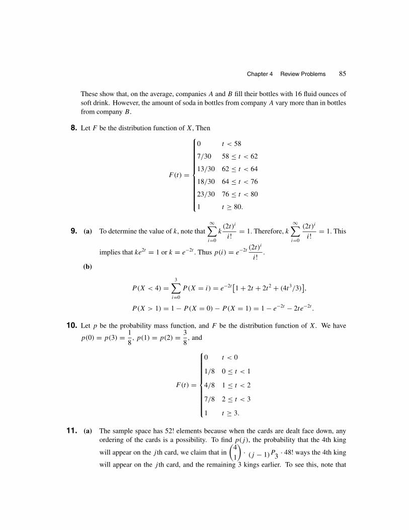
Chapter 4 Review Problems 85
These show that, on the average, companies A and B fill their bottles with 16 fluid ounces ofsoft drink. However, the amount of soda in bottles from company A vary more than in bottlesfrom company B.
8. Let F be the distribution function of X, Then
F(t) =
⎧⎪⎪⎪⎪⎪⎪⎪⎪⎪⎪⎪⎨⎪⎪⎪⎪⎪⎪⎪⎪⎪⎪⎪⎩
0 t < 58
7/30 58 ≤ t < 62
13/30 62 ≤ t < 64
18/30 64 ≤ t < 76
23/30 76 ≤ t < 80
1 t ≥ 80.
9. (a) To determine the value of k, note that∞∑i=0
k(2t)i
i! = 1. Therefore, k
∞∑i=0
(2t)i
i! = 1. This
implies that ke2t = 1 or k = e−2t . Thus p(i) = e−2t (2t)i
i! .
(b)
P(X < 4) =3∑
i=0
P(X = i) = e−2t[1 + 2t + 2t2 + (4t3/3)
],
P (X > 1) = 1 − P(X = 0) − P(X = 1) = 1 − e−2t − 2te−2t .
10. Let p be the probability mass function, and F be the distribution function of X. We have
p(0) = p(3) = 1
8, p(1) = p(2) = 3
8, and
F(t) =
⎧⎪⎪⎪⎪⎪⎪⎪⎪⎪⎨⎪⎪⎪⎪⎪⎪⎪⎪⎪⎩
0 t < 0
1/8 0 ≤ t < 1
4/8 1 ≤ t < 2
7/8 2 ≤ t < 3
1 t ≥ 3.
11. (a) The sample space has 52! elements because when the cards are dealt face down, anyordering of the cards is a possibility. To find p(j), the probability that the 4th king
will appear on the j th card, we claim that in
(4
1
)· (j − 1)P3 · 48! ways the 4th king
will appear on the j th card, and the remaining 3 kings earlier. To see this, note that

86 Chapter 4 Distribution Functions and Discrete Random Variables
we have
(4
1
)combinations for the king that appears on the j th card, and (j − 1)P3
different permutations for the remaining 3 kings that appear earlier. The last term 48!,is for the remaining 48 cards that can appear in any order in the remaining 48 positions.Therefore,
p(j) =
(4
1
)· (j − 1)P3 · 48!
52! =
(j − 1
3
)52!
4! 48!=
(j − 1
3
)(
52
4
) .
(b) The probability that the player wins is p(52) =(
51
3
)/(52
4
)= 1/13.
(c) To find
E =52∑
j=4
jp(j) = 1(52
4
) 52∑j=4
j
(j − 1
3
),
the expected length of the game, we use a technique introduced by Jenkyns and Mullerin Mathematics Magazine, 54, (1981), page 203. We have the following relation whichcan be readily checked.
j
(j − 1
3
)= 4
5
[(j + 1)
(j
4
)− j
(j − 1
4
)], j ≥ 5.
This gives
52∑j=5
j
(j − 1
3
)=4
5
[ 52∑j=5
(j + 1)
(j
4
)−
52∑j=5
j
(j − 1
4
)]
= 4
5
[53
(52
4
)− 5
(4
4
)]= 11, 478, 736,
where the next-to-the-last equality follows because terms cancel out in pairs. Thus
E = 1(52
4
) 52∑j=4
j
(j − 1
3
)= 1(
52
4
)[4 +52∑
j=5
j
(j − 1
3
)]
= 1(52
4
)(4 + 11, 478, 736) = 42.4.
As Jenkyns and Muller have noted, “This relatively high expectation value is what makes thegame interesting. However, the low probability of winning makes it frustrating!”

Chapter 5
Special Discrete
Distributions
5.1 BERNOULLI AND BINOMIAL RANDOM VARIABLES
1.(
8
4
)(1
4
)4(3
4
)4 = 0.087.
2. (a) 64 × 1
2= 32.
(b) 6 × 1
2+ 1 = 4 (note that we should count the mother of the family as well).
3.(
6
3
)(1
6
)3(5
6
)3 = 0.054.
4.(
6
2
)( 1
10
)2( 9
10
)4 = 0.098.
5.(
5
2
)(10
30
)2(20
30
)3 = 0.33.
6. Let X be the number of defective nails. If the manufacturer’s claim is true, we have
P(X ≥ 2) = 1 − P(X = 0) − P(X = 1)
= 1 −(
24
0
)(0.03)0(0.97)24 −
(24
1
)(0.03)(0.97)23 = 0.162.
This shows that there is 16.2% chance that two or more defective nails is found. Therefore, itis not fair to reject company’s claim.
7. Let p and q be the probability mass functions of X and Y , respectively. Then
p(x) =(
4
x
)(0.60)x(0.40)4−x, x = 0, 1, 2, 3, 4;

88 Chapter 5 Special Discrete Distributions
q(y) = P(Y = y) = P(X = y − 1
2
)=(
4y−1
2
)(0.60)(y−1)/2(0.40)4−[(y−1)/2], y = 1, 3, 5, 7, 9.
8.8∑
i=0
(15
i
)(0.8)i(0.2)15−i = 0.142.
9.(
10
5
)(11
36
)5(25
36
)5 = 0.108.
10. (a) 1 −(
5
0
)(1
3
)0(2
3
)5 −(
5
1
)(1
3
)1(2
3
)4 = 0.539. (b)(
5
2
)( 1
10
)2( 9
10
)3 = 0.073.
11. We know that p(x) is maximum at [(n + 1)p]. If (n + 1)p is an integer, p(x) is maximum at[(n + 1)p] = np + p. But in such a case, some straightforward algebra shows that(
n
np + p
)pnp+p(1 − p)n−np−p =
(n
np + p − 1
)pnp+p−1(1 − p)n−np−p+1,
implying that p(x) is also maximum at np + p − 1.
12. The probability of royal or straight flush is 40/(52
5
). If Ernie plays n games, he will get, on
the average, n
[40/(52
5
)]royal or straight flushes. We want to have 40n
/(52
5
)= 1; this
gives n =(
52
5
)/40 = 64, 974.
13.(
6
3
)(1
3
)3(2
3
)3 = 0.219.
14. 1 − (999/1000)100 = 0.095.
15. The maximum occurs at k = [11(0.45)] = 4. The maximum probability is(10
4
)(0.45)4(0.55)6 = 0.238.
16. Call the event of obtaining a full house success. X, the number of full houses is n independentpoker hands is a binomial random variable with parameters (n, p), where p is the probability
that a random poker hand is a full house. To calculate p, note that there are
(52
5
)possible
poker hands and
(4
3
)(4
2
)13!11! = 3744 full houses. Thus p = 3744
/(52
5
)≈ 0.0014. Hence

Section 5.1 Bernoulli and Binomial Random Variables 89
E(X) = np ≈ 0.0014n and Var(X) = np(1−p) ≈ 0.00144n. Note that if n is approximately715, then E(X) = 1. Thus we should expect to find, on the average, one full house in every715 random poker hands.
17. 1 −(
6
6
)(1
4
)6(3
4
)0 −(
6
5
)(1
4
)5(3
4
)≈ 0.995.
18. 1 −(
3000
0
)(0.0005)0(0.9995)3000 −
(3000
1
)(0.0005)(0.9995)2999 ≈ 0.442.
19. The expected value of the expenses if sent in one parcel is
45.20 × 0.07 + 5.20 × 0.93 = 8.
The expected value of the expenses if sent in two parcels is
(23.30 × 2)(0.07)2 + (23.30 + 3.30)
(2
1
)(0.07)(0.93) + (6.60)(0.93)2 = 9.4.
Therefore, it is preferable to send in a single parcel.
20. Let n be the minimum number of children they should plan to have. Since the probability of allgirls is (1/2)n and the probability of all boys is (1/2)n, we must have 1−(1/2)n−(1/2)n ≥ 0.95.
This gives (1/2)n−1 ≤ 0.05 or n − 1 ≥ ln 0.05
ln(0.5)= 4.32 or n ≥ 5.32. Therefore, n = 6.
21. (a) For this to happen, exactly one of the N stations has to attempt transmitting a message.
The probability of this is
(N
1
)p(1 − p)N−1 = Np(1 − p)N−1.
(b) Let f (p) = Np(1−p)N−1. The value of p which maximizes the probability of a messagegoing through with no collision is the root of the equation f
′(p) = 0. Now
f′(p) = N(1 − p)N−1 − Np(N − 1)(1 − p)N−2 = 0.
Noting that p �= 1, this equation gives p = 1/N. This answer makes a lot of sense because atevery “suitable instance,” on average, Np = 1 station will transmit a message.
(c) By part (b), the maximum probability is
f( 1
N
)= N
( 1
N
)(1 − 1
N
)N−1 =(
1 − 1
N
)N−1.
As N → ∞, this probability approaches 1/e, showing that for large numbers of stations(in reality 20 or more), the probability of a successful transmission is approximately 1/e
independently of the number of stations if p = 1/N .

90 Chapter 5 Special Discrete Distributions
22. The k students whose names have been called are not standing. Let A1, A2, . . . , An−k be thestudents whose names have not been called. For i, 1 ≤ i ≤ n − k, call Ai a “success,” if he orshe is standing; failure, otherwise. Therefore, whether Ai is standing or sitting is a Bernoullitrial, and hence the random variable X is the number of successes in n − k Bernoulli trials.For X to be binomial, for i �= j , the event that Ai is a success must be independent of theevent that Aj is a success. Furthermore, the probability that Ai is a success must be the samefor all i, 1 ≤ i ≤ n − k. The latter condition is satisfied since Ai is standing if and only if hisoriginal seat was among the first k. This happens with probability p = k/n regardless of i .However, the former condition is not valid. The relation
P(Aj is standing | Ai is standing
) = k − 1
n,
shows that given Ai is a success changes the probability that Aj is success. That is, Ai being asuccess is not independent of Aj being a success. This shows that X is not a binomial randomvariable.
23. Let X be the number of undecided voters who will vote for abortion. The desired probabilityis
P(b + (n − X) > a + X
) = P(X <
n + (b − a)
2
)=
[n+(b−a)
2 ]∑i=0
(n
i
)(1
2
)i(1
2
)n−i
=(1
2
)n[n+(b−a)
2 ]∑i=0
(n
i
).
24. Let X be the net gain of the player per unit of stake. X is a discrete random variable withpossible values −1, 1, 2, and 3. We have
P(X = −1) =(
3
0
)(1
6
)0(5
6
)3 = 125
216,
P (X = 1) =(
3
1
)(1
6
)(5
6
)2 = 75
216,
P (X = 2) =(
3
2
)(1
6
)2(5
6
)= 15
216,
P (X = 3) =(
3
3
)(1
6
)3(5
6
)0 = 1
216.
Hence
E(X) = −1 · 125
216+ 1 · 75
216+ 2 · 15
216+ 3 · 1
216≈ −0.08.
Therefore, the player loses 0.08 per unit stake.

Section 5.1 Bernoulli and Binomial Random Variables 91
25.
E(X2) =n∑
x=1
x2
(n
x
)px(1 − p)n−x =
n∑x=1
(x2 − x + x)
(n
x
)px(1 − p)n−x
=n∑
x=1
x(x − 1)
(n
x
)px(1 − p)n−x +
n∑x=1
x
(n
x
)px(1 − p)n−x
=n∑
x=2
n!(x − 2)! (n − x)! px(1 − p)n−x + E(X)
= n(n − 1)p2n∑
x=2
(n − 2
x − 2
)px−2(1 − p)n−x + np
= n(n − 1)p2[p + (1 − p)
]n−2 + np = n2p2 − np2 + np.
26. (a) A four-engine plane is preferable to a two-engine plane if and only if
1 −(
4
0
)p0(1 − p)4 −
(4
1
)p(1 − p)3 > 1 −
(2
0
)p0(1 − p)2.
This inequality gives p > 2/3. Hence a four-engine plane is preferable if and only if p > 2/3.If p = 2/3, it makes no difference.(b) A five-engine plane is preferable to a three-engine plane if and only if(
5
5
)p5(1 − p)0 +
(5
4
)p4(1 − p) +
(5
3
)p3(1 − p)2 >
(3
2
)p2(1 − p) + p3.
Simplifying this inequality, we get 3(p − 1)2(2p − 1) ≥ 0 which implies that a five-engineplane is preferable if and only if 2p − 1 ≥ 0. That is, for p > 1/2, a five-engine plane ispreferable; for p < 1/2, a three-engine plane is preferable; for p = 1/2 it makes no difference.
27. Clearly, 8 bits are transmitted. A parity check will not detect an error in the 7–bit characterreceived erroneously if and only if the number of bits received incorrectly is even. Therefore,the desired probability is
4∑n=1
(8
2n
)(1 − 0.999)2n(0.999)8−2n = 0.000028.
28. The message is erroneously received but the errors are not detected by the parity-check if for1 ≤ j ≤ 6, j of the characters are erroneously received but not detected by the parity–check,and the remaining 6−j characters are all transmitted correctly. By the solution of the previousexercise, the probability of this event is
6∑j=1
(0.000028)j (0.999)8(6−j) = 0.000161.

92 Chapter 5 Special Discrete Distributions
29. The probability of a straight flush is 40/(52
5
)≈ 0.000015391. Hence we must have
1 −(
n
0
)(0.000015391)0(1 − 0.000015391)n ≥ 3
4.
This gives
(1 − 0.000015391)n ≤ 1
4.
So
n ≥ log(1/4)
log(1 − 0.000015391)≈ 90071.06.
Therefore, n ≈ 90, 072.
30. Let p, q, and r be the probabilities that a randomly selected offspring is AA, Aa, and aa,respectively. Note that both parents of the offspring are AA with probability (α/n)2, they areboth Aa with probability
[1 − (α/n)
]2, and the probability is 2(α/n)
[1 − (α/n)
]that one
parent is AA and the other is Aa. Therefore, by the law of total probability,
p = 1 ·(α
n
)2 + 1
4·(
1 − α
n
)2 + 1
2· 2(α
n
)(1 − α
n
)= 1
4
(α
n
)2 + 1
2
(α
n
)+ 1
4,
q = 0 ·(α
n
)2 + 1
2
(1 − α
n
)2 + 1
2· 2(α
n
)(1 − α
n
)= 1
2− 1
2
(α
n
)2,
r = 0 ·(α
n
)2 + 1
4
(1 − α
n
)2 + 0 · 2(α
n
)(1 − α
n
)= 1
4
(1 − α
n
)2.
The probability that at most two of the offspring are aa is
2∑i=0
(m
i
)ri(1 − r)m−i .
The probability that exactly i of the offspring are AA and the remaining are all Aa is(m
i
)piqm−i .
31. The desired probability is the sum of three probabilities: probability of no customer served andtwo new arrivals, probability of one customer served and three new arrivals, and probabilityof two customers served and four new arrivals. These quantities, respectively, are (0.4)4 ·(
4
2
)(0.45)2(0.55)2,
(4
1
)(0.6)(0.4)3 ·
(4
3
)(0.45)3(0.55), and
(4
2
)(0.6)2(0.4)2 · (0.45)4. The
sum of these quantities, which is the answer, is 0.054.

Section 5.1 Bernoulli and Binomial Random Variables 93
32. (a) Let S be the event that the first trial is a success and E be the event that in n trials, thenumber of successes is even. Then
P(E) = P(E|S)P (S) + P(E|Sc)P (Sc).
Thusrn = (1 − rn−1)p + rn−1(1 − p).
Using this relation, induction, and r0 = 1, we find that
rn = 1
2
[1 + (1 − 2p)n
].
(b) The left sum is the probability of 0, 2, 4, . . . , or [n/2] successes. Thus it is the probabilityof an even number of successes in n Bernoulli trials and hence it is equal to rn.
33. For 0 ≤ i ≤ n, let Bi be the event that i of the balls are red. Let A be the event that in drawingk balls from the urn, successively, and with replacement, no red balls appear. Then
P(B0|A) = P(A|B0)P (B0)n∑
i=0
P(A|Bi)P (Bi)
=1 ×
(1
2
)n
n∑i=0
(n − i
n
)k(
n
i
)(1
2
)n= 1
n∑i=0
(n
i
)(n − i
n
)k.
34. Let E be the event that Albert’s statement is the truth and F be the event that Donna tells thetruth. Since Rose agrees with Donna and Rose always tells the truth, Donna is telling the truthas well. Therefore, the desired probability is P(E | F) = P(EF)/P (F ). To calculate P(F),observe that for Rose to agree with Donna, none, two, or all four of Albert, Brenda, Charles,and Donna should have lied. Since these four people lie independently, this will happen withprobability (1
3
)4 +(
4
2
)(2
3
)2(1
3
)2 +(2
3
)4 = 41
81.
To calculate P(EF), note that EF is the event that Albert tells the truth and Rose agrees withDonna. This happens if all of them tell the truth, or Albert tells the truth but exactly two ofBrenda, Charles and Donna lie. Hence
P(EF) =(1
3
)4 + 1
3·(
3
2
)(2
3
)2(1
3
)= 13
81.
Therefore,
P(E | F) = P(EF)
P (F )= 13/81
41/81= 13
41= 0.317.

94 Chapter 5 Special Discrete Distributions
5.2 POISSON RANDOM VARIABLES
1. λ = (0.05)(60) = 3; the answer is 1 − e−330
0! = 1 − e−3 = 0.9502.
2. λ = 1.8; the answer is∑3
i=0
e−1.8(1.8)i
i! ≈ 0.89.
3. λ = 0.025 × 80 = 2; the answer is 1 − e−220
0! − e−221
1! = 1 − 3e−2 = 0.594.
4. λ = (500)(0.0014) = 0.7. The answer is 1 − e−0.7(0.7)0
0! − e−0.7(0.7)1
1! ≈ 0.156.
5. We call a room “success” if it is vacant next Saturday; we call it “failure” if it is occupied.Assuming that next Saturday is a random day, X, the number of vacant rooms on that day isapproximately Poisson with rate λ = 35. Thus the desired probability is
1 −29∑i=0
e−35(35)i
i! = 0.823.
6. λ = (3/10)35 = 10.5. The probability of 10 misprints in a given chapter ise−10.5(10.5)10
10! =0.124. Therefore, the desired probability is (0.124)2 = 0.0154.
7. P(X = 1) = P(X = 3) implies that e−λλ = e−λ λ3
3! from which we get λ = √6. The answer
ise−√
6(√
6)5
5! = 0.063.
8. The probability that a bun contains no raisins ise−n/k(n/k)0
0! = e−n/k. So the answer is(4
2
)e−2n/k(1 − e−n/k)2.
9. Let X be the number of times the randomly selected kid has hit the target. We are given that
P(X = 0) = 0.04; this implies thate−λ20
0! = 0.04 or e−λ = 0.04. So λ = − ln 0.04 = 3.22.
Now
P(X ≥ 2) = 1 − P(X = 0) − P(X = 1) = 1 − 0.04 − e−λ λ
1!= 1 − 0.04 − (0.04)(3.22) = 0.83.
Therefore, 83% of the kids have hit the target at least twice.

Section 5.2 Poisson Random Variables 95
10. First we calculate pi’s from binomial probability mass function with n = 26 and p = 1/365.Then we calculate them from Poisson probability mass function with parameter λ = np =26/365. For different values of i, the results are as follows.
i Binomial Poisson0 0.93115 0.931251 0.06651 0.066342 0.00228 0.002363 0.00005 0.00006.
Remark: In this example, since success is very rare, even for small n’s Poisson gives goodapproximation for binomial. The following table demonstrates this fact for n = 5.
i Binomial Poisson0 0.9874 0.98641 0.0136 0.01362 0.00007 0.00009.
11. Let N(t) be the number of shooting stars observed up to time t . Let one minute be the unit oftime. Then
{N(t) : t ≥ 0
}is a Poisson process with λ = 1/12. We have that
P(N(30) = 3
) = e−30/12(30/12)3
3! = 0.21.
12. P(N(2) = 0
) = e−3(2) = e−6 = 0.00248.
13. Let N(t) be the number of wrong calls up to t . If one day is taken as the time unit, it is reasonableto assume that
{N(t) : t ≥ 0
}is a Poisson process with λ = 1/7. By the independent increment
property and stationarity, the desired probability is
P(N(1) = 0
) = e−(1/7)·1 = 0.87.
14. Choose one month as the unit of time. Then λ = 5 and the probability of no crimes duringany given month of a year is P
(N(1) = 0
) = e−5 = 0.0067. Hence the desired probability is(12
2
)(0.0067)2(1 − 0.0067)10 = 0.0028.
15. Choose one day as the unit of time. Then λ = 3 and the probability of no accidents in one dayis
P(N(1) = 0
)= e−3 = 0.0498.
The number of days without any accidents in January is approximately another Poisson randomvariable with approximate rate 31(0.05) = 1.55. Hence the desired probability is
e−1.55(1.55)3
3! ≈ 0.13.

96 Chapter 5 Special Discrete Distributions
16. Choosing one hours as time unit, we have that λ = 6. Therefore, the desired probability is
P(N(0.5) = 1 and N(2.5) = 10
) = P(N(0.5) = 1 and N(2.5) − N(0.5) = 9
)= P
(N(0.5) = 1
)P(N(2.5) − N(0.5) = 9
)= P
(N(0.5) = 1
)P(N(2) = 9
)= 31e−3
1! · 129e−12
9! ≈ 0.013.
17. The expected number of fractures per meter is λ = 1/60. Let N(t) be the number of fracturesin t meters of wire. Then
P(N(t) = n
) = e−t/60(t/60)n
n! , n = 0, 1, 2, . . . .
In a ten minute period, the machine turns out 70 meters of wire. The desired probability,P(N(70) > 1
)is calculated as follows:
P(N(70) > 1
) = 1 − P(N(70) = 0
)− P(N(70) = 1
)= 1 − e−70/60 − 70
60e−70/60 ≈ 0.325.
18. Let the epoch at which the traffic light for the left–turn lane turns red be labeled t = 0. LetN(t) be the number of cars that arrive at the junction at or prior to t trying to turn left. Sincecars arrive at the junction according to a Poisson process, clearly,
{N(t) : t ≥ 0
}is a stationary
and orderly process which possesses independent increments. Therefore,{N(t) : t ≥ 0
}is
also a Poisson process. Its parameter is given by λ = E[N(1)
] = 4(0.22) = 0.88. (For arigorous proof, see the solution to Exercise 9, Section 12.2.) Thus
P(N(t) = n
) = e−(0.88)t[(0.88)t
]nn! ,
and the desired probability is
P(N(3) ≥ 4
) = 1 −3∑
n=0
e−(0.88)3[(0.88)3
]nn! ≈ 0.273.
19. Let X be the number of earthquakes of magnitude 5.5 or higher on the Richter scale during thenext 60 years. Clearly, X is a Poisson random variable with parameter λ = 6(1.5) = 9. Let A
be the event that the earthquakes will not damage the bridge during the next 60 years. Sincethe events {X = i}, i = 0, 1, 2, . . . , are mutually exclusive and
⋃∞i=1{X = i} is the sample
space, by the Law of Total Probability (Theorem 3.4),
P(A) =∞∑i=0
P(A | X = i)P (X = i) =∞∑i=0
(1 − 0.015)i e−9 9i
i!
=∞∑i=0
(0.985)i e−9 9i
i! = e−9∞∑i=0
[(0.985)(9)
]ii! = e−9e(0.985)(9) = 0.873716.
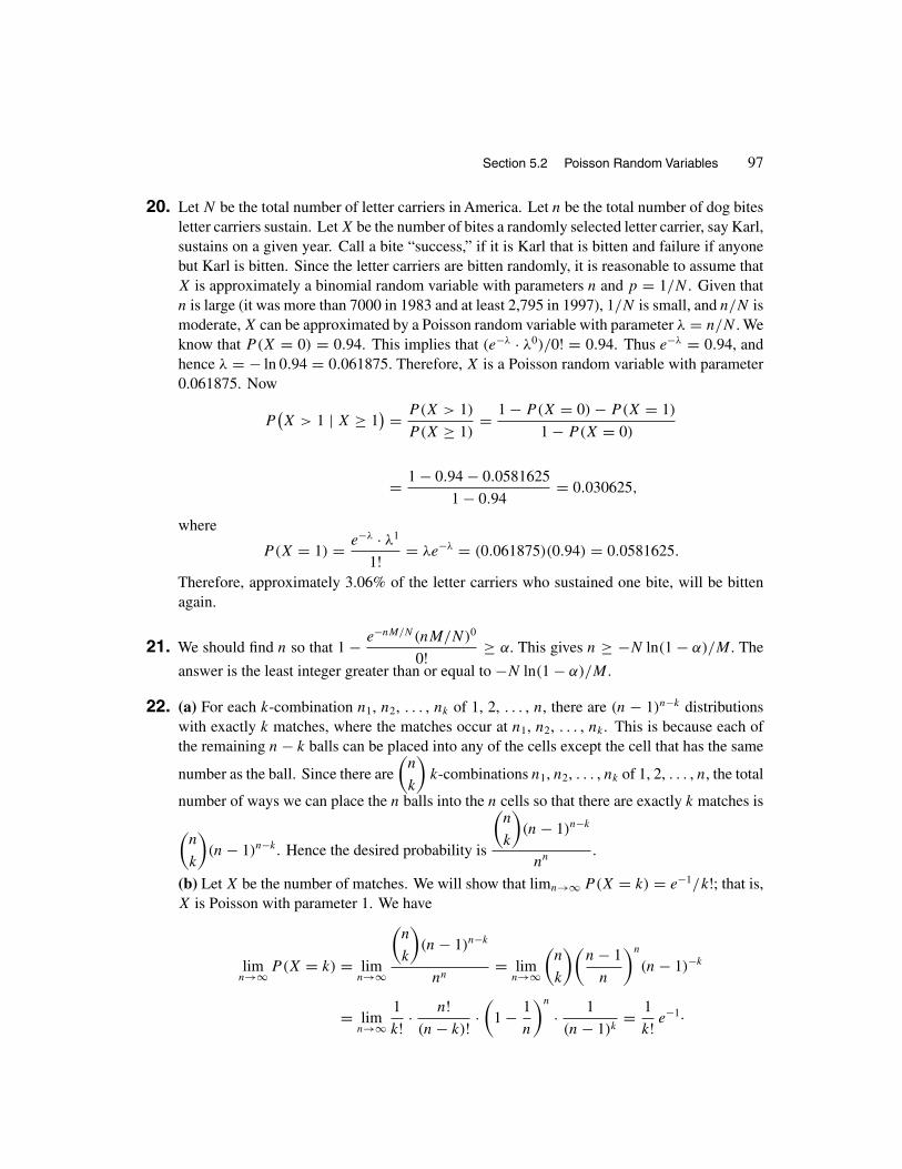
Section 5.2 Poisson Random Variables 97
20. Let N be the total number of letter carriers in America. Let n be the total number of dog bitesletter carriers sustain. Let X be the number of bites a randomly selected letter carrier, say Karl,sustains on a given year. Call a bite “success,” if it is Karl that is bitten and failure if anyonebut Karl is bitten. Since the letter carriers are bitten randomly, it is reasonable to assume thatX is approximately a binomial random variable with parameters n and p = 1/N . Given thatn is large (it was more than 7000 in 1983 and at least 2,795 in 1997), 1/N is small, and n/N ismoderate, X can be approximated by a Poisson random variable with parameter λ = n/N. Weknow that P(X = 0) = 0.94. This implies that (e−λ · λ0)/0! = 0.94. Thus e−λ = 0.94, andhence λ = − ln 0.94 = 0.061875. Therefore, X is a Poisson random variable with parameter0.061875. Now
P(X > 1 | X ≥ 1
) = P(X > 1)
P (X ≥ 1)= 1 − P(X = 0) − P(X = 1)
1 − P(X = 0)
= 1 − 0.94 − 0.0581625
1 − 0.94= 0.030625,
where
P(X = 1) = e−λ · λ1
1! = λe−λ = (0.061875)(0.94) = 0.0581625.
Therefore, approximately 3.06% of the letter carriers who sustained one bite, will be bittenagain.
21. We should find n so that 1 − e−nM/N(nM/N)0
0! ≥ α. This gives n ≥ −N ln(1 − α)/M. The
answer is the least integer greater than or equal to −N ln(1 − α)/M.
22. (a) For each k-combination n1, n2, . . . , nk of 1, 2, . . . , n, there are (n − 1)n−k distributionswith exactly k matches, where the matches occur at n1, n2, . . . , nk. This is because each ofthe remaining n − k balls can be placed into any of the cells except the cell that has the same
number as the ball. Since there are
(n
k
)k-combinations n1, n2, . . . , nk of 1, 2, . . . , n, the total
number of ways we can place the n balls into the n cells so that there are exactly k matches is(n
k
)(n − 1)n−k. Hence the desired probability is
(n
k
)(n − 1)n−k
nn .
(b) Let X be the number of matches. We will show that limn→∞ P(X = k) = e−1/k!; that is,X is Poisson with parameter 1. We have
limn→∞ P(X = k) = lim
n→∞
(n
k
)(n − 1)n−k
nn= lim
n→∞
(n
k
)(n − 1
n
)n
(n − 1)−k
= limn→∞
1
k! · n!(n − k)! ·
(1 − 1
n
)n
· 1
(n − 1)k= 1
k! e−1·
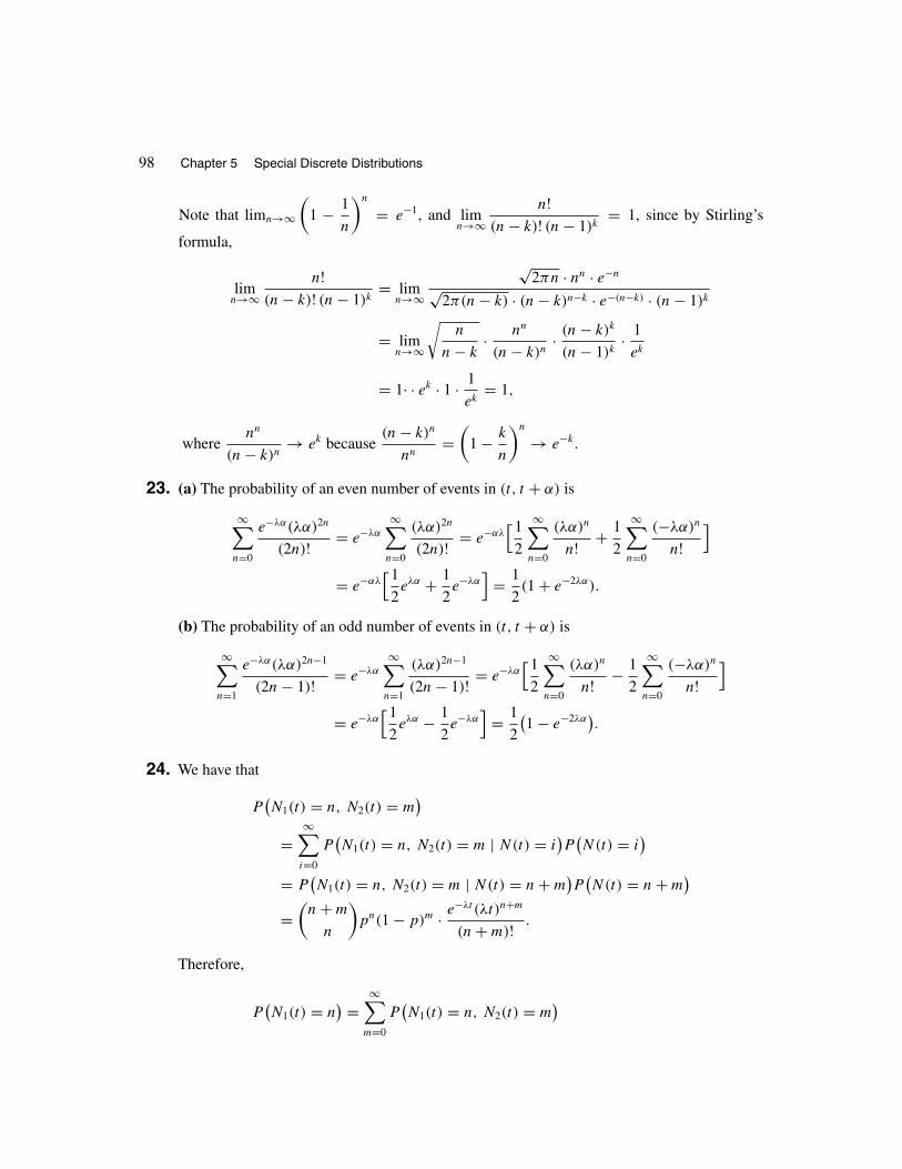
98 Chapter 5 Special Discrete Distributions
Note that limn→∞(
1 − 1
n
)n
= e−1, and limn→∞
n!(n − k)! (n − 1)k
= 1, since by Stirling’s
formula,
limn→∞
n!(n − k)! (n − 1)k
= limn→∞
√2πn · nn · e−n
√2π(n − k) · (n − k)n−k · e−(n−k) · (n − 1)k
= limn→∞
√n
n − k· nn
(n − k)n· (n − k)k
(n − 1)k· 1
ek
= 1· · ek · 1 · 1
ek= 1,
wherenn
(n − k)n→ ek because
(n − k)n
nn=(
1 − k
n
)n
→ e−k.
23. (a) The probability of an even number of events in (t, t + α) is
∞∑n=0
e−λα(λα)2n
(2n)! = e−λα
∞∑n=0
(λα)2n
(2n)! = e−αλ[1
2
∞∑n=0
(λα)n
n! + 1
2
∞∑n=0
(−λα)n
n!]
= e−αλ[1
2eλα + 1
2e−λα
]= 1
2(1 + e−2λα).
(b) The probability of an odd number of events in (t, t + α) is
∞∑n=1
e−λα(λα)2n−1
(2n − 1)! = e−λα
∞∑n=1
(λα)2n−1
(2n − 1)! = e−λα[1
2
∞∑n=0
(λα)n
n! − 1
2
∞∑n=0
(−λα)n
n!]
= e−λα[1
2eλα − 1
2e−λα
]= 1
2
(1 − e−2λα
).
24. We have that
P(N1(t) = n, N2(t) = m
)=
∞∑i=0
P(N1(t) = n, N2(t) = m | N(t) = i
)P(N(t) = i
)= P
(N1(t) = n, N2(t) = m | N(t) = n + m
)P(N(t) = n + m
)=(
n + m
n
)pn(1 − p)m · e−λt (λt)n+m
(n + m)! .
Therefore,
P(N1(t) = n
) =∞∑
m=0
P(N1(t) = n, N2(t) = m
)

Section 5.3 Other Discrete Random Variables 99
=∞∑
m=0
(n + m
n
)pn(1 − p)m · e−λt (λt)n+m
(n + m)!
=∞∑
m=0
(n + m)!n! m! pn(1 − p)m e−λtpe−λt (1−p)(λt)n(λt)m
(n + m)!
=∞∑
m=0
e−λtpe−λt (1−p)(λtp)n[λt (1 − p)
]mn! m!
= e−λtp(λtp)n
n!∞∑
m=0
e−λt (1−p)[λt (1 − p)
]mm!
= e−λtp(λtp)n
n! .
It can easily be argued that the other properties of Poisson process are also satisfied for theprocess
{N1(t) : t ≥ 0
}. So
{N1(t) : t ≥ 0
}is a Poisson process with rate λp. By symmetry,{
N2(t) : t ≥ 0}
is a Poisson process with rate λ(1 − p).
25. Let N(t) be the number of females entering the store between 0 and t . By Exercise 24,{N(t) : t ≥ 0
}is a Poisson process with rate 1 · (2/3) = 2/3. Hence the desired probability is
P(N(15) = 15
) = e−15(2/3)[15(2/3)
]15
15! = 0.035.
26. (a) Let A be the region whose points have a (positive) distance d or less from the given tree.The desired probability is the probability of no trees in this region and is equal to
e−λπd2(λπd 2)0
0! = e−λπd2.
(b) We want to find the probability that the region A has at most n − 1 trees. The desiredquantity is
n−1∑i=0
e−λπd2(λπd 2)i
i! .
27. p(i) = (λ/i)p(i − 1) implies that for i < λ, the function p is increasing and for i > λ it isdecreasing. Hence i = [λ] is the maximum.
5.3 OTHER DISCRETE RANDOM VARIABLES
1. Let D denote a defective item drawn, and N denote a nondefective item drawn. The answeris S = {
NNN, DNN, NDN, NND, NDD, DND, DDN}.

100 Chapter 5 Special Discrete Distributions
2. S = {ss, f ss, sf s, sff s, ff ss, f sf s, sfff s, f sff s, fff ss, ff sf s, . . .
}.
3. (a) 1/(1/12) = 12. (b)(11
12
)2( 1
12
)≈ 0.07.
4. (a) (1 − pq)r−1pq. (b) 1/pq.
5.(
7
2
)(0.2)3(0.8)5 ≈ 0.055.
6. (a) (0.55)5(0.45) ≈ 0.023. (b) (0.55)3(0.45)(0.55)3(0.45) ≈ 0.0056.
7.[(5
1
)(45
7
)]/(50
8
)= 0.42.
8. The probability that at least n light bulbs are required is equal to the probability that the firstn − 1 light bulbs are all defective. So the answer is pn−1.
9. We have
P(N = n)
P (X = x)=
(n − 1
x − 1
)px(1 − p)n−x(
n
x
)px(1 − p)n−x
= x
n.
10. Let X be the number of the words the student had to spell until spelling a word correctly. Therandom variable X is geometric with parameter 0.70. The desired probability is given by
P(X ≤ 4) =4∑
i=1
(0.30)i−1(0.70) = 0.9919.
11. The average number of digits until the fifth 3 is 5/(1/10) = 50. So the average number ofdigits before the fifth 3 is 49.
12. The probability that a random bridge hand has three aces is
p =
(4
3
)(48
10
)(
52
13
) = 0.0412.
Therefore, the average number of bridge hands until one has three aces is 1/p = 1/0.0412 =24.27.
13. Either the (N + 1)st success must occur on the (N + M − m + 1)st trial, or the (M + 1)st

Section 5.3 Other Discrete Random Variables 101
failure must occur on the (N + M − m + 1)st trial. The answer is(N + M − m
N
)(1
2
)N+M−m+1 +(
N + M − m
M
)(1
2
)N+M−m+1.
14. We have that X + 10 is negative binomial with parameters (10, 0.15). Therefore, ∀i ≥ 0,
P(X = i) = P(X + 10 = i + 10) =(
i + 9
9
)(0.15)10(0.85)i .
15. Let X be the number of good diskettes in the sample. The desired probability is
P(X ≥ 9) = P(X = 9) + P(X = 10) =
(10
1
)(90
9
)(
100
10
) +
(90
10
)(10
0
)(
100
10
) ≈ 0.74.
16. We have that 560(0.35) = 196 persons make contributions. So the answer is
1 −
(364
15
)(
560
15
) −
(364
14
)(196
1
)(
560
15
) = 0.987.
17. The transmission of a message takes more than t minutes, if the first [t/2] + 1 times it is sentit will be garbled, where [t/2] is the greatest integer less than or equal to t/2. The probabilityof this is p[t/2]+1.
18. The probability that the sixth coin is accepted on the nth try is(n − 1
5
)(0.10)6(0.90)n−6.
Therefore, the desired probability is
∞∑n=50
(n − 1
5
)(0.10)6(0.90)n−6 = 1 −
49∑n=6
(n − 1
5
)(0.10)6(0.90)n−6 = 0.6346.
19. The probability that the station will successfully transmit or retransmit a message is (1−p)N−1.
This is because for the station to successfully transmit or retransmit its message, none of theother stations should transmit messages at the same instance. The number of transmissionsand retransmissions of a message until the success is geometric with parameter (1 − p)N−1.Therefore, on average, the number of transmissions and retransmissions is 1/(1 − p)N−1.

102 Chapter 5 Special Discrete Distributions
20. If the fifth tail occurs after the 14th trial, ten or more heads have occurred. Therefore, the fifthtail occurs before the tenth head if and only if the fifth tail occurs before or on the 14th flip.Calling tails success, X, the number of flips required to get the fifth tail is negative binomialwith parameters 5 and 1/2. The desired probability is given by
14∑n=5
P(X = n) =14∑
n=5
(n − 1
4
)(1
2
)5(1
2
)n−5 ≈ 0.91.
21. The probability of a straight is
10(45)− 40(
52
5
) = 0.003924647.
Therefore, the expected number of poker hands required until the first straight is1/0.003924647 = 254.80.
22. (a) SinceP(X = n − 1)
P (X = n)= 1
1 − p> 1,
P (X = n) is a decreasing function of n; hence its maximum is at n = 1.
(b) The probability that X is even is given by
∞∑k=1
P(X = 2k) =∞∑
k=1
p(1 − p)2k−1 = p(1 − p)
1 − (1 − p)2= 1 − p
2 − p.
(c) We want to show the following:
Let X be a discrete random variable with the set of possible values{1, 2, 3 . . .
}.
If for all positive integers n and m,
P(X > n + m | X > m) = P(X > n), (17)
then X is a geometric random variable. That is, there exists a number p,0 < p < 1, such that
P(X = n) = p(1 − p)n−1. (18)
To prove this, note that (17) implies that for all positive integers n and m,
P(X > n + m)
P (X > m)= P(X > n).
Therefore,
P(X > n + m) = P(X > n)P (X > m). (19)

Section 5.3 Other Discrete Random Variables 103
Let p = P(X = 1); using induction, we prove that (18) is valid for all positive integers n. Toshow (18) for n = 2, note that (19) implies that
P(X > 2) = P(X > 1)P (X > 1).
Since P(X > 1) = 1 − P(X = 1) = 1 − p, this relation gives
1 − P(X = 1) − P(X = 2) = (1 − p)2,
or1 − p − P(X = 2) = (1 − p)2,
which yieldsP(X = 2) = p(1 − p),
so (18) is also true for n = 2. Now assume that (18) is valid for all positive integers i, i ≤ n;that is, assume that
P(X = i) = p(1 − p)i−1, i ≤ n. (20)
We will show that (18) is true for n + 1. The induction hypothesis [relation (20)] implies that
P(X ≤ n) =n∑
i=1
P(X = i) =n∑
i=1
p(1 − p)i−1 = p1 − (1 − p)n
1 − (1 − p)= 1 − (1 − p)n.
So P(X > n) = (1 − p)n and, similarly, P(X > n − 1) = (1 − p)n−1. Now (19) yields
P(X > n + 1) = P(X > n)P (X > 1),
which implies that
1 − P(X ≤ n) − P(X = n + 1) = (1 − p)n(1 − p).
Substituting P(X ≤ n) = 1 − (1 − p)n in this relation, we obtain
P(X = n + 1) = p(1 − p)n,
which establishes (18) for n + 1. Therefore, we have what we wanted to show.
23. Consider a coin for which the probability of tails is 1 − p and the probability of heads is p.In successive and independent flips of the coin, let X1 be the number of flips until the firsthead, X2 be the total number of flips until the second head, X3 be the total number of flipsuntil the third head, and so on. Then the length of the first character of the message and X1
are identically distributed. The total number of the bits forming the first two characters ofthe message and X2 are identically distributed. The total number of the bits forming the firstthree characters of the message and X3 are identically distributed, and so on. Therefore, thetotal number of the bits forming the message has the same distribution as Xk. This is negativebinomial with parameters k and p.

104 Chapter 5 Special Discrete Distributions
24. Let X be the number of cartons to be opened before finding one without rotten eggs. X is not ageometric random variable because the number of cartons is limited, and one carton not havingrotten eggs is not independent of another carton not having rotten eggs. However, it should be
obvious that a geometric random variable with parameter p =(
1000
12
)/(1200
12
)= 0.1109 is
a good approximation for X. Therefore, we should expect approximately 1/p = 1/0.1109 =9.015 cartons to be opened before finding one without rotten eggs.
25. Either the N th success should occur on the (2N − M)th trial or the N th failure should occuron the (2N − M)th trial. By symmetry, the answer is
2 ·(
2N − M − 1
N − 1
)(1
2
)N(1
2
)N−M =(
2N − M − 1
N − 1
)(1
2
)2N−M−1.
26. The desired quantity is 2 times the probability of exactly N successes in (2N − 1) trials andfailures on the (2N)th and (2N + 1)st trials:
2
(2N − 1
N
)(1
2
)N(1 − 1
2
)(2N−1)−N ·(
1 − 1
2
)2 =(
2N − 1
N
)(1
2
)2N
.
27. Let X be the number of rolls until Adam gets a six. Let Y be the number of rolls of the dieuntil Andrew rolls an odd number. Since the events (X = i), 1 ≤ i < ∞, form a partition ofthe sample space, by Theorem 3.4,
P(Y > X
) =∞∑i=1
P(Y > X | X = i
)P(X = i
) =∞∑i=1
P(Y > i
)P(X = i
)
=∞∑i=1
(1
2
)i ·(5
6
)i−1 1
6= 6
5· 1
6
∞∑i=1
( 5
12
)i = 1
5·
5
12
1 − 5
12
= 1
7,
where P(Y > i) = (1/2)i since for Y to be greater than i, Andrew must obtain an even numberon each of the the first i rolls.
28. The probability of 4 tagged trout among the second 50 trout caught is
pn =
(50
4
)(n − 50
46
)(
n
50
) .
It is logical to find the value of n for which pn is maximum. (In statistics this value is calledthe maximum likelihood estimate for the number of trout in the lake.) To do this, note that
pn
pn−1= (n − 50)2
n(n − 96).

Section 5.3 Other Discrete Random Variables 105
Now pn ≥ pn−1 if and only if (n − 50)2 ≥ n(n − 96), or n ≤ 625. Therefore, n = 625 makespn maximum, and hence there are approximately 625 trout in the lake.
29. (a) Intuitively, it should be clear that the answer is D/N . To prove this, let Ej be the event ofobtaining exactly j defective items among the first (k − 1) draws. Let Ak be the event that thekth item drawn is defective. We have
P(Ak) =k−1∑j=0
P(Ak | Ej)P (Ej) =k−1∑j=0
D − j
N − k + 1·
(D
j
)(N − D
k − 1 − j
)(
N
k − 1
) .
Now
(D − j)
(D
j
)= D
(D − 1
j
)and
(N − k + 1)
(N
k − 1
)= N
(N − 1
k − 1
).
Therefore,
P(Ak) =k−1∑j=0
D
(D − 1
j
)(N − D
k − 1 − j
)N
(N − 1
k − 1
) = D
N
k−1∑j=0
(D − 1
j
)(N − D
k − 1 − j
)(
N − 1
k − 1
) = D
N,
where
k−1∑j=0
(D − 1
j
)(N − D
k − 1 − j
)(
N − 1
k − 1
) = 1
since
(D − 1
j
)(N − D
k − 1 − j
)(
N − 1
k − 1
) is the probability mass function of a hypergeometric random
variable with parameters N − 1, D − 1, and k − 1.(b) Intuitively, it should be clear that the answer is (D − 1)/(N − 1). To prove this, let Ak beas before and let Fj be the event of exactly j defective items among the first (k − 2) draws.Let B be the event that the (k − 1)st and the kth items drawn are defective. We have
P(B) =k−2∑j=0
P(B | Fj)P (Fj )

106 Chapter 5 Special Discrete Distributions
=k−2∑j=0
(D − j)(D − j − 1)
(N − k + 2)(N − k + 1)·
(D
j
)(N − D
k − 2 − j
)(
N
k − 2
)
=k−2∑j=0
D(D − 1)
(D − 2
j
)(N − D
k − 2 − j
)N(N − 1)
(N − 2
k − 2
)
= D(D − 1)
N(N − 1)
k−2∑j=0
(D − 2
j
)(N − D
k − 2 − j
)(
N − 2
k − 2
)= D(D − 1)
N(N − 1).
Using this, we have that the desired probability is
P(Ak | Ak−1) = P(AkAk−1)
P (Ak−1)= P(B)
P (Ak−1)=
D(D − 1)
N(N − 1)
D
N
= D − 1
N − 1.
REVIEW PROBLEMS FOR CHAPTER 5
1.20∑
i=12
(20
i
)(0.25)i(0.75)20−i = 0.0009.
2. N(t), the number of customers arriving at the post office at or prior to t is a Poisson processwith λ = 1/3. Thus
P(N(30) ≤ 6
) =6∑
i=0
P(N(30) = i
) =6∑
i=0
e−(1/3)30[(1/3)30
]ii! = 0.130141.
3. 4 · 8
30= 1.067.
4.2∑
i=0
(12
i
)(0.30)i(0.70)12−i = 0.253.

Chapter 5 Review Problems 107
5.(
5
2
)(0.18)2(0.82)3 = 0.179.
6.1999∑i=2
(i − 1
2 − 1
)( 1
1000
)2( 999
1000
)i−2 = 0.59386.
7.12∑i=7
(160
i
)(200
12 − i
)(
360
12
) = 0.244.
8. Call a train that arrives between 10:15 A.M. and 10:28 A.M. a success. Then p, the probabilityof success is
p = 28 − 15
60= 13
60.
Therefore, the expected value and the variance of the number of trains that arrive in the givenperiod are 10(13/60) = 2.167 and 10(13/60)(47/60) = 1.697, respectively.
9. The number of checks returned during the next two days is Poisson with λ = 6. The desiredprobability is
P(X ≤ 4) =4∑
i=0
e−6 6i
i! = 0.285.
10. Suppose that 5% of the items are defective. Under this hypothesis, there are 500(0.05) = 25defective items. The probability of two defective items among 30 items selected at random is(
25
2
)(475
28
)(
500
30
) = 0.268.
Therefore, under the above hypothesis, having two defective items among 30 items selectedat random is quite probable. The shipment should not be rejected.
11. N is a geometric random variable with p = 1/2. So E(N) = 1/p = 2, and Var(N) =(1 − p)/p2 = [
1 − (1/2)]/(1/4) = 2.
12.(5
6
)5(1
6
)= 0.067.
13. The number of times a message is transmitted or retransmitted is geometric with parameter1 − p. Therefore, the expected value of the number of transmissions and retransmissions of a

108 Chapter 5 Special Discrete Distributions
message is 1/(1 − p). Hence the expected number of retransmissions of a message is
1
1 − p− 1 = p
1 − p.
14. Call a customer a “success,” if he or she will make a purchase using a credit card. Let E
be the event that a customer entering the store will make a purchase. Let F be the event thatthe customer will use a credit card. To find p, the probability of success, we use the law ofmultiplication:
p = P(EF) = P(E)P(F | E
) = (0.30)(0.85) = 0.255.
The random variable X is binomial with parameters 6 and 0.255. Hence
P(X = i
) =(
6
i
)(0.255
)i(1 − 0.255
)6−i, i = 0, 1, . . . , 6.
Clearly, E(X) = np = 6(0.255) = 1.53 and
Var(X) = np(1 − p) = 6(0.255)(1 − 0.255) = 1.13985.
15.5∑
i=3
(18
i
)(10
5 − i
)(
28
5
) = 0.772.
16. By the formula for the expected value of a hypergeometric random variable, the desired quantityis (5 × 6)/16 = 1.875.
17. We want to find the probability that at most 4 of the seeds do not germinate:
4∑i=0
(40
i
)(0.06)i(0.94)40−i = 0.91.
18. 1 −2∑
i=0
(20
i
)(0.06)i(0.94)20−i = 0.115.
Let X be the number of requests for reservations at the end of the second day. It is reasonableto assume that X is Poisson with parameter 3 × 3 × 2 = 18. Hence the desired probability is
P(X ≥ 24) = 1 −23∑i=0
P(X = i) = 1 −23∑i=0
e−18 (18)i
i! = 1 − 0.89889 = 0.10111.

Chapter 5 Review Problems 109
19. Suppose that the company’s claim is correct. Then the probability of 12 or less drivers usingseat belts regularly is
12∑i=0
(20
i
)(0.70)i(0.30)20−i ≈ 0.228.
Therefore, under the assumption that the company’s claim is true, it is quite likely that out of20 randomly selected drivers, 12 use seat belts. This is not a reasonable evidence to concludethat the insurance company’s claim is false.
20. (a) (0.999)999(0.001)1 = 0.000368. (b)(
2999
2
)(0.001)3(0.999)2997 = 0.000224.
21. Let X be the number of children having the disease. We have that the desired probability is
P(X = 3 | X ≥ 1) = P(X = 3)
P (X ≥ 1)=
(5
3
)(0.23)3(0.77)2
1 − (0.77)5= 0.0989.
22. (a)( w
w + b
)n−1( b
w + b
). (b)
( w
w + b
)n−1.
23. Let n be the desired number of seeds to be planted. Let X be the number of seeds whichwill germinate. We have that X is binomial with parameters n and 0.75. We want to find thesmallest n for which
P(X ≥ 5) ≥ 0.90.
or, equivalently,
P(X < 5) ≤ 0.10.
That is, we want to find the smallest n for which
4∑i=0
(n
i
)(0.75)i(.25)n−i ≤ 0.10.
By trial and error, as the following table shows, we find that the smallest n satisfyingP(X < 5) ≤ 0.10 is 9. So at least nine seeds is to be planted.
n∑4
i=0
(n
i
)(0.75)i(.25)n−i
5 0.7627
6 0.46617 0.24368 0.11399 0.0489

110 Chapter 5 Special Discrete Distributions
24. Intuitively, it must be clear that the answer is k/n. To prove this, let B be the event that the ithbaby born is blonde. Let A be the event that k of the n babies are blondes. We have
P(B | A) = P(AB)
P (A)=
p ·(
n − 1
k − 1
)pk−1(1 − p)n−k(
n
k
)pk(1 − p)n−k
=
(n − 1
k − 1
)(
n
k
) = k
n.
25. The size of a seed is a tiny fraction of the size of the area. Let us divide the area up into manysmall cells each about the size of a seed. Assume that, when the seeds are distributed, eachof them will land in a single cell. Accordingly, the number of seeds distributed will equalthe number of nonempty cells. Suppose that each cell has an equal chance of having a seedindependent of other cells (this is only approximately true). Since λ is the average number ofseeds per unit area, the expected number of seeds in the area, A, is λA. Let us call a cell inA a “success” if it is occupied by a seed. Let n be the total number of cells in A and p bethe probability that a cell will contain a seed. Then X, the number of cells in A with seedsis a binomial random variable with parameters n and p. Using the formula for the expectednumber of successes in a binomial distribution (= np), we see that np = λA and p = λA/n.As n goes to infinity, p approaches zero while np remains finite. Hence the number of seedsthat fall on the area A is a Poisson random variable with parameter λA and
P(X = i) = e−λA(λA)i
i! .
26. Let D/N → p, then by the Remark 5.2, for all n,(D
x
)(N − D
n − x
)(
N
n
) ≈(
n
x
)px(1 − p)n−x.
Now since n → ∞ and nD/N → λ, n is large and np is appreciable, thus(n
x
)px(1 − p)n−x ≈ e−λλx
x! .

Chapter 6
Continuous Random
Variables
6.1 PROBABILITY DENSITY FUNCTIONS
1. (a)∫ ∞
0ce−3x dx = 1 �⇒ c = 3.
(b) P(0 < X ≤ 1/2) =∫ 1/2
03e−3x dx = 1 − e−3/2 ≈ 0.78.
2. (a) f (x) =⎧⎨⎩
32
x3x ≥ 4
0 x < 4.
(b) P(X ≤ 5) = 1 − (16/25) = 9/25,
P (X ≥ 6) = 16/36 = 4/9,
P (5 ≤ X ≤ 7) = [1 − (16/49)
]− [1 − (16/25)
] = 0.313,
P (1 ≤ X < 3.5) = 0 − 0 = 0.
3. (a)∫ 2
1c(x − 1)(2 − x) dx = 1 �⇒ c
[− x3
3+ 3x2
2− 2x
]2
1= 1 �⇒ c = 6.
(b) F(x) =∫ x
16(x − 1)(2 − x) dx, 1 ≤ x < 2. Thus
F(x) =
⎧⎪⎨⎪⎩0 x < 1
−2x3 + 9x2 − 12x + 5 1 ≤ x < 2
1 x ≥ 2.
(c) P(X < 5/4) = F(5/4) = 5/32,
P (3/2 ≤ X ≤ 2) = F(2) − F(3/2) = 1 − (1/2) = 1/2.
4. (a) P(X < 1.5) =∫ 1.5
1
2
x2dx = 2
3.

112 Chapter 6 Continuous Random Variables
(b) P(1 < X < 1.25 | X < 1.5) =
∫ 1.25
1
2
x2dx∫ 1.5
1
2
x2dx
= 2/5
2/3= 3
5.
5. (a)∫ 1
−1
c√1 − x2
dx = 1 �⇒[c · arcsin x
]1
−1= 1 �⇒ c = 1/π.
(b) For −1 < x < 1,
F(x) =∫ x
−1
1
π√
1 − x2dx = 1
πarcsin x + 1
2.
Thus
F(x) =
⎧⎪⎪⎪⎪⎨⎪⎪⎪⎪⎩0 x < −1
1
πarcsin x + 1
2−1 ≤ x < 1
1 x ≥ 1.
6. Since h(x) ≥ 0 and∫ ∞
α
f (x)
1 − F(α)dx = 1
1 − F(α)
∫ ∞
α
f (x) dx = 1
1 − F(α)
[1 − F(α)
] = 1,
h is a probability density function.
7. (a) Let F be the distribution function of X. Then X is symmetric about α if and only if for allx, 1 − F(α + x) = F(α − x), or upon differentiation f (α + x) = f (α − x).
(b) f (α + x) = f (α − x) if and only if (α − x − 3)2 = (α + x − 3)2. This is true for all x, ifand only if α − x − 3 = −(α + x − 3) which gives α = 3. A similar argument shows that g
is symmetric about α = 1.
8. (a) Since f is a probability density function,∫ ∞
−∞f (x) dx = 1. But
∫ ∞
−∞f (x) dx =
∫ 0
−1k(2x − 3x2) dx = k
∫ 0
−1(2x − 3x2) dx = k
[x2 − x3
]0
−1= −2k.
So −2k = 1 or k = −1/2.
(b) The loss is at most $500 if and only if X ≥ −1/2. Therefore, the desired probability is
P(X ≥ −1
2
)=∫ 0
−1/2−1
2(2x − 3x2) dx = −1
2
[x2 − x3
]0
−1/2= 3
16.

Section 6.2 Density Function of a Function of a Random Variable 113
9. P(X > 15) =∫ ∞
15
1
15e−x/15 dx = 1
e. Thus the answer is
8∑i=4
(8
i
)(1
e
)i(1 − 1
e
)8−i = 0.3327.
10. Since αf + βg ≥ 0 and∫ ∞
−∞
[αf (x) + βg(x)
]dx = α
∫ ∞
−∞f (x) dx + β
∫ ∞
−∞g(x) dx = α + β = 1,
αf + βg is also a probability density function.
11. Since F(−∞) = 0 and F(∞) = 1, We have that{α + β(−π/2) = 0
α + β(π/2) = 1.
Solving this system of two equations in two unknown, we obtain α = 1/2 and β = 1/π. Thus
f (x) = F ′(x) = 2
π(4 + x2), −∞ < x < ∞.
6.2 DENSITY FUNCTION OF A FUNCTION OF A RANDOM VARIABLE
1. Let G be the distribution function of Y ; for −8 < y < 8,
G(y) = P(Y ≤ y) = P(X3 ≤ y) = P(X ≤ 3√
y ) =∫ 3√y
−2
1
4dx = 1
43√
y + 1
2.
Therefore,
G(y) =
⎧⎪⎪⎪⎪⎨⎪⎪⎪⎪⎩0 y < −8
1
43√
y + 1
2−8 ≤ y < 8
1 y ≥ 8.
This gives
g(y) = G′(y) =
⎧⎪⎨⎪⎩1
12y−2/3 −8 < y < 8
0 otherwise.
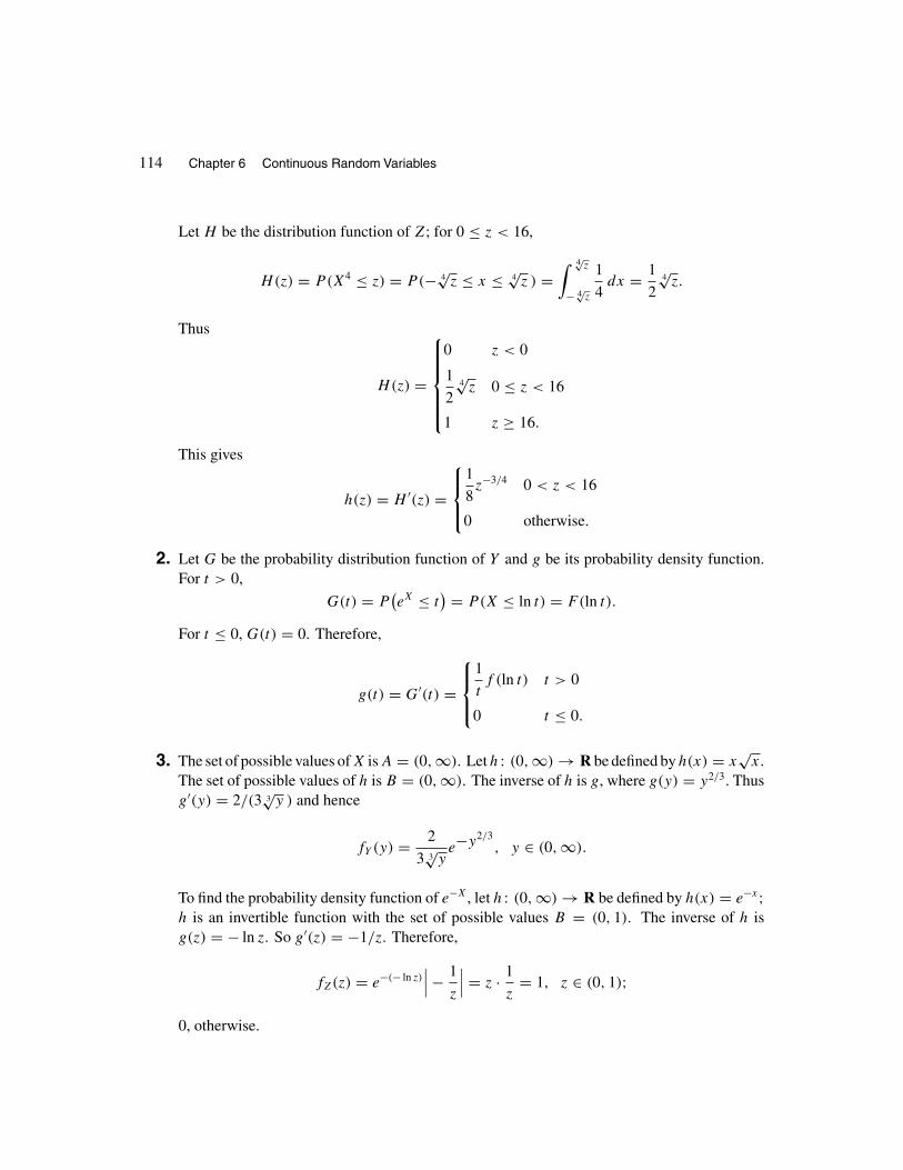
114 Chapter 6 Continuous Random Variables
Let H be the distribution function of Z; for 0 ≤ z < 16,
H(z) = P(X4 ≤ z) = P(− 4√
z ≤ x ≤ 4√
z ) =∫ 4√z
− 4√z
1
4dx = 1
24√
z.
Thus
H(z) =
⎧⎪⎪⎪⎪⎨⎪⎪⎪⎪⎩0 z < 0
1
24√
z 0 ≤ z < 16
1 z ≥ 16.
This gives
h(z) = H ′(z) =
⎧⎪⎨⎪⎩1
8z−3/4 0 < z < 16
0 otherwise.
2. Let G be the probability distribution function of Y and g be its probability density function.For t > 0,
G(t) = P(eX ≤ t
) = P(X ≤ ln t) = F(ln t).
For t ≤ 0, G(t) = 0. Therefore,
g(t) = G′(t) =
⎧⎪⎨⎪⎩1
tf (ln t) t > 0
0 t ≤ 0.
3. The set of possible values of X is A = (0, ∞). Let h : (0, ∞) → R be defined by h(x) = x√
x.
The set of possible values of h is B = (0, ∞). The inverse of h is g, where g(y) = y2/3. Thusg′(y) = 2/(3 3
√y ) and hence
fY (y) = 2
3 3√
ye−y2/3
, y ∈ (0, ∞).
To find the probability density function of e−X, let h : (0, ∞) → R be defined by h(x) = e−x;h is an invertible function with the set of possible values B = (0, 1). The inverse of h isg(z) = − ln z. So g′(z) = −1/z. Therefore,
fZ(z) = e−(− ln z)∣∣∣− 1
z
∣∣∣ = z · 1
z= 1, z ∈ (0, 1);
0, otherwise.
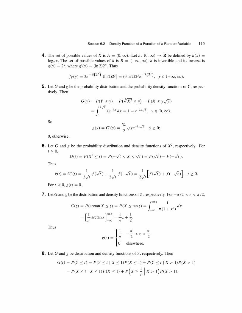
Section 6.2 Density Function of a Function of a Random Variable 115
4. The set of possible values of X is A = (0, ∞). Let h : (0, ∞) → R be defined by h(x) =log2 x. The set of possible values of h is B = (−∞, ∞). h is invertible and its inverse isg(y) = 2y , where g′(y) = (ln 2)2y . Thus
fY (y) = 3e−3(2y)∣∣(ln 2)2y
∣∣ = (3 ln 2)2ye−3(2y), y ∈ (−∞, ∞).
5. Let G and g be the probability distribution and the probability density functions of Y , respec-tively. Then
G(y) = P(Y ≤ y) = P( 3√
X2 ≤ y) = P(X ≤ y
√y )
=∫ y
√y
0λe−λx dx = 1 − e−λy
√y, y ∈ [0, ∞).
So
g(y) = G′(y) = 3λ
2√
ye−λy√
y, y ≥ 0;0, otherwise.
6. Let G and g be the probability distribution and density functions of X2, respectively. Fort ≥ 0,
G(t) = P(X2 ≤ t) = P(−√t < X <
√t ) = F(
√t ) − F(−√
t ).
Thus
g(t) = G ′(t) = 1
2√
tf (
√t ) + 1
2√
tf (−√
t ) = 1
2√
t
[f (
√t ) + f (−√
t )], t ≥ 0.
For t < 0, g(t) = 0.
7. Let G and g be the distribution and density functions of Z, respectively. For −π/2 < z < π/2,
G(z) = P(arctan X ≤ z) = P(X ≤ tan z) =∫ tan z
−∞1
π(1 + x2)dx
=[ 1
πarctan x
]tan z
−∞= 1
πz + 1
2.
Thus
g(z) =
⎧⎪⎨⎪⎩1
π−π
2< z <
π
2
0 elsewhere.
8. Let G and g be distribution and density functions of Y , respectively. Then
G(t) = P(Y ≤ t) = P(Y ≤ t | X ≤ 1)P (X ≤ 1) + P(Y ≤ t | X > 1)P (X > 1)
= P(X ≤ t | X ≤ 1)P (X ≤ 1) + P(X ≥ 1
t
∣∣∣ X > 1)P(X > 1).

116 Chapter 6 Continuous Random Variables
For t ≥ 1, this gives
G(t) = 1 ·∫ 1
0e−x dx + 1 ·
∫ ∞
1e−x dx = 1.
For 0 < t < 1, this gives
G(t) = P(X ≤ t) + P(X ≥ 1
t
)=∫ t
0e−x dx +
∫ ∞
1/t
e−x dx = 1 − e−t + e−1/t .
Hence
G(t) =
⎧⎪⎨⎪⎩0 t ≤ 0
1 − e−t + e−1/t 0 < t < 1
1 t ≥ 1.
Therefore,
g(t) = G′(t) =
⎧⎪⎨⎪⎩e−t + 1
t2e−1/t 0 < t < 1
0 elsewhere.
6.3 EXPECTATIONS AND VARIANCES
1. The probability density function of X is f (x) =⎧⎨⎩32/x3 x ≥ 4
0 x < 4.Thus
(a) E(X) =∫ ∞
4
32
x2dx = 8.
(b) E(X2) =∫ ∞
4
32
xdx = ∞; so Var(X) = E(X2) − [
E(X)]2
does not exist.
2. (a) E(X) = 6∫ 2
1(−x3 + 3x2 − 2x) dx = 3
2.
(b) E(X2) = 6∫ 2
1(−x4 +3x3 −2x2) dx = 23
10; so Var(X) = 23
10− 9
4= 1
20, and σX = 1√
20.
3. The standardized value of the lifetime of a car muffler manufactured by company A is(4.25−5)/2 = −0.375. The corresponding value for company B is (3.75−4)/1.5 = −0.167.
Therefore, the muffler of company B has performed relatively better.
4. E(eX) =
∫ ∞
0ex(3e−3x) dx =
∫ ∞
03e−2x dx = 3/2.

Section 6.3 Expectations and Variances 117
5. E(X) =∫ 1
−1
x
π√
1 − x2dx = 0, because the integrand is an odd function.
6. Let f be the probability density function of Y . Clearly,
f (y) = F′(y) =
⎧⎪⎪⎨⎪⎪⎩k
Ae−k(α−y)/A −∞ < y ≤ α
0 y > α.
Therefore,
E(Y ) =∫ α
−∞k
Aye−k(α−y)/A dy = k
Ae−kα/A
[A
kyeky/A − A2
k2eky/A
]α
−∞= α − A
k.
7. Let H be the distribution function of C; then
P(F ≤ t) = P(C ≤ t − 32
1.8
)= H
( t − 32
1.8
).
Hence the probability density function of F is
d
dtP (F ≤ t) = 1
1.8h( t − 32
1.8
)= 5
9h( t − 32
1.8
).
The expected value of F is given by
E(F) = 1.8E(C) + 32 = 1.8∫ ∞
−∞xh(x) dx + 32.
8. E(ln X) =∫ 2
1
2 ln x
x2dx. To calculate this integral, let U = ln x, dV = 1/x2, and use
integration by parts:∫ 2
1
2 ln x
x2dx = −2 ln x
x
∣∣∣∣21
−∫ 2
1− 2
x2dx = 1 − ln 2 = 0.3069.
9. The expected value of the length of the other side is given by
E(√
81 − X2) =
∫ 4
2
√81 − x2 · x
6dx.
Letting u = 81 − x2, we get du = −2x dx and
E(√
81 − X2) = 1
12
∫ 77
65
√u du ≈ 8.4.

118 Chapter 6 Continuous Random Variables
10. E(X) =∫ ∞
−∞1
2xe−|x| dx = 0, because the integrand is an odd function. Now
E(X2) =∫ ∞
−∞1
2x2e−|x| dx =
∫ ∞
0x2e−x dx
since the integrand is an even function; applying integration by parts to the last integral twice,we obtain E(X2) = 2. Hence Var(X) = 2 − 02 = 2.
11. Note that
E(|X|α) =
∫ ∞
−∞|x|α
π(1 + x2)dx = 2
π
∫ ∞
0
xα
(1 + x2)dx
since the integrand is an even function. Now for 0 < α < 1,∫ ∞
0
xα
1 + x2dx =
∫ 1
0
xα
1 + x2dx +
∫ ∞
1
xα
1 + x2dx.
Clearly, the first integral in the right side is convergent. To show that the second one is alsoconvergent, note that.
xα
1 + x2≤ xα
x2= 1
x2−α.
Therefore, ∫ ∞
1
xα
1 + x2dx ≤
∫ ∞
1
1
x2−αdx =
[ 1
(α − 1)x1−α
]∞1
= 1
1 − α< ∞.
For α ≥ 1,∫ ∞
0
xα
1 + x2≥∫ ∞
1
xα
1 + x2dx ≥
∫ ∞
1
x
1 + x2dx =
[1
2ln(1 + x2)
]∞1
= ∞.
So∫ ∞
0
xα
1 + x2dx diverges.
12. By Remark 6.4,
E(X) =∫ ∞
0P(X > t) dt =
∫ ∞
0(αe−λt + βe−µt ) dt = α
λ+ β
µ.
13. (a) c1 is an arbitrary positive number because ∀c1,∫ ∞
c1
c1
x2dx = 1. For n > 1,
∫ ∞
cn
cn
xn+1dx =
1 implies that cn = n−1/(n−1).
(b) E(Xn) =∫ ∞
cn
cn
xndx =
⎧⎨⎩∞ if n = 1
n(n−2)/(n−1)/(n − 1) if n > 1.
(c) P(Zn ≤ t) = P(ln Xn ≤ t) = P(Xn ≤ et ) =∫ et
cn
cn
xn+1dx = cn
n
[ 1
cnn
− 1
ent
], where

Section 6.3 Expectations and Variances 119
cn = n−1/(n−1). Let gn be the probability density function of Zn. Then gn(t) = cne−nt ,
t ≥ ln cn.
(d) E(Xm+1n ) =
∫ ∞
cn
cnxm+1
xn+1dx. This integral exists if and only if m − n < −1.
14. Using integration by parts twice, we obtain
E(Xn+1) = 1
π
∫ π
0xn+2 sin x dx = πn+1 + (n + 2)
1
π
∫ π
0xn+1 cos x dx
= πn+1 + (n + 2)[
− (n + 1)1
π
∫ π
0xn sin x dx
]= πn+1 + (n + 2)
[− (n + 1)E(Xn−1)].
HenceE(Xn+1) + (n + 1)(n + 2)E(Xn−1) = πn+1.
15. Since X is symmetric about α, for all x ∈ (−∞, ∞), f (α+x) = f (α−x). Letting y = x+α,we have
E(X) =∫ ∞
−∞yf (y) dy =
∫ ∞
−∞(x + α)f (x + α) dx
=∫ ∞
−∞xf (x + α) dx + α
∫ ∞
−∞f (x + α) dx.
Now since f is symmetric about α, xf (x + α) is an odd function,
−xf (−x + α) = −[xf (x + α)].
Therefore,∫ ∞
−∞xf (x + α) = 0. Since
∫ ∞
−∞f (x + α) dx =
∫ ∞
−∞f (y) dy = 1, we have
E(X) = 0 + α · 1 = α.
To show that the median of X is α, we will show that P(X ≤ α) = P(X ≥ α). This alsoshows that the value of these two probabilities is 1/2. Letting u = α − x, we have
P(X ≤ α) =∫ α
−∞f (x) dx =
∫ ∞
0f (α − u) du.
Letting u = x − α, we have that
P(X ≥ α) =∫ ∞
α
f (x) dx =∫ ∞
0f (u + α) du.

120 Chapter 6 Continuous Random Variables
Since for all u,
f (α − u) = f (α + u),
we have thatP(X ≤ α) = P(X ≥ α) = 1/2.
16. By Theorem 6.3,
E(|X − y|) =
∫ ∞
−∞|x − y|f (x)dx =
∫ y
−∞(y − x)f (x) dx +
∫ ∞
y
(x − y)f (x) dx
= y
∫ y
−∞f (x) dx −
∫ y
−∞xf (x) dx +
∫ ∞
y
xf (x) dx − y
∫ ∞
y
f (x) dx.
Hence
dE(|X − y|)
dy=∫ y
−∞f (x) dx + yf (y) − yf (y) − yf (y) −
∫ ∞
y
f (x) dx + yf (y)
=∫ y
−∞f (x) dx −
∫ ∞
y
f (x) dx.
SettingdE(|X − y|)
dy= 0, we obtain that y is the solution of the following equation:∫ y
−∞f (x) dx =
∫ ∞
y
f (x) dx.
By the definition of the median of a continuous random variable, the solution to this equationis y = median(X). Hence E
(|X − y|) is minimum for y = median(X).
17. (a)∫ ∞
0I (t) dt =
∫ X
0I (t) dt +
∫ ∞
X
I (t) dt =∫ X
0dt +
∫ ∞
X
0 dt = X.
(Note that∫ ∞
0I (t) dt is a random variable.)
(b) E(X) = E[ ∫ ∞
0I (t) dt
]=∫ ∞
0E[I (t)
]dt =
∫ ∞
0P(X > t) dt =
∫ ∞
0
[1 − F(t)
]dt.
(c) By part (b),
E(Xr) =∫ ∞
0P(Xr > t) dt =
∫ ∞
0P(X >
r√
t)dt
=∫ ∞
0
[1 − F
(r√
t)]
dt = r
∫ ∞
0yr−1
[1 − F(y)
]dy,
where the last equality follows by the substitution y = r√
t .

Section 6.3 Expectations and Variances 121
18. On the interval [n, n + 1),
P(|X| ≥ n + 1
) ≤ P(|X| > t
) ≤ P(|X| ≥ n
).
Therefore,∫ n+1
n
P(|X| ≥ n + 1
)dt ≤
∫ n+1
n
P(|X| > t
)dt ≤
∫ n+1
n
P(|X| ≥ n
)dt,
or
P(|X| ≥ n + 1
) ≤∫ n+1
n
P(|X| > t
)dt ≤ P
(|X| ≥ n).
So ∞∑n=0
P(|X| ≥ n + 1
) ≤∞∑
n=0
∫ n+1
n
P(|X| > t
)dt ≤
∞∑n=0
P(|X| > n
),
and hence ∞∑n=1
P(|X| ≥ n
) ≤ E(|X|) ≤ 1 +
∞∑n=1
P(|X| ≥ n
).
19. By Exercise 12,
E(X) = α
λ+ β
µ.
Using Exercise 16, we obtain
E(X2) = 2∫ ∞
0x(αe−λx + βe−µx) dx = 2α
λ2+ 2β
µ2.
Hence
Var(X) =(2α
λ2+ 2β
µ2
)−(α
λ+ β
µ
)2 = 2α − α2
λ2+ 2β − β2
µ2− 2αβ
λµ.
20. X ≥st Y implies that for all t ,
P(X > t) ≥ P(Y > t). (21)
Taking integrals of both sides of (21) yields,∫ ∞
0P(X > t) dt ≥
∫ ∞
0P(Y > t) dt. (22)
Relation (21) also implies that
1 − P(X ≤ t) ≥ 1 − P(Y ≤ t),
or, equivalently,P(X ≤ t) ≤ P(Y ≤ t)·

122 Chapter 6 Continuous Random Variables
Since this is true for all t , we have
P(X ≤ −t) ≤ P(Y ≤ −t)·
Taking integrals of both sides of this inequality, we have∫ ∞
0P(X ≤ −t) ≤
∫ ∞
0P(Y ≤ −t) dt,
or, equivalently,
−∫ ∞
0P(X ≤ −t) ≥ −
∫ ∞
0P(Y ≤ −t) dt. (23)
Adding (22) and (23) yields∫ ∞
0P(X > t) dt −
∫ ∞
0P(X ≤ −t) dt ≥
∫ ∞
0P(Y > t) dt −
∫ ∞
0P(Y ≤ −t) dt ·
By Theorem 6.2, this gives E(X) ≥ E(Y ). To show that the converse of this theorem is false,let X and Y be discrete random variables both with set of possible values {1, 2, 3}. Let theprobability mass functions of X and Y be defined by
pX(1) = 0.3 pX(2) = 0.4 pX(3) = 0.3
pY (1) = 0.5 pY (2) = 0.1 pY (3) = 0.4
We have that E(X) = 2 > E(Y ) = 1.9. However, since
P(X > 2) = 0.3 < P(Y > 2) = 0.4,
we see that X is not stochastically larger than Y .
21. First, we show that limx→−∞ xP(X ≤ x
) = 0. To do so, since x → −∞, we concentrate onnegative values of x. Letting u = −t , we have
xP(X ≤ x
) = x
∫ x
−∞f (t) dt = x
∫ ∞
−x
f (−u) du = −∫ ∞
−x
−xf (−u) du.
So it suffices to show that as x → −∞,∫∞−x
−xf (−u) du → 0. Now∫ ∞
−x
−xf (−u) du ≤∫ ∞
−x
uf (−u) du.
Therefore, it remains to prove that∫∞−x
uf (−u) du → 0 as x → −∞. But this is true because∫ ∞
−∞|u|f (−u) du =
∫ ∞
−∞|x|f (x) dx < ∞.

Chapter 6 Review Problems 123
Next, we will show that limx→∞ xP(X > x
) = 0. To do so, note that
limx→∞ xP
(X > x
) = limx→∞ x
∫ ∞
x
f (t) dt ≤ limx→∞
∫ ∞
x
tf (t) dt = 0
since∫∞−∞ |tf (t)| dt < ∞.
REVIEW PROBLEMS FOR CHAPTER 6
1. Let F be the distribution function of Y . Clearly, F(y) = 0 if y ≤ 1. For y > 1,
F(y) = P( 1
X≤ y
)= P
(X ≥ 1
y
)=
1 − 1
y
1 − 0= 1 − 1
y.
So
f (y) = F ′(y) =⎧⎨⎩1/y2 y > 1
0 elsewhere.
2. E(X) =∫ ∞
1x · 2
x3dx =
∫ ∞
1
2
x2dx = −2
x
∣∣∣∣∞1
= 2,
E(X2) =∫ ∞
1x2 · 2
x3dx = 2 ln x
∣∣∣∞1
= ∞. So Var(X) does not exist.
3. E(X) =∫ 1
0(6x2 − 6x3) dx =
[2x3 − 6
4x4]1
0= 1
2,
E(X2) =∫ 1
0(6x3 − 6x4) dx =
[6
4x4 − 6
5x5]1
0= 3
10,
Var(X) = 3
10−(1
2
)2 = 1
20, σX = 1
2√
5.
Therefore,
P(1
2− 2
2√
5< X <
1
2+ 2
2√
5
)=∫ 1
2 + 1√5
12 − 1√
5
(6x − 6x2) dx
=[
3x2 − 2x3
] 12 + 1√
5
12 − 1√
5
= 11
5√
5.

124 Chapter 6 Continuous Random Variables
4. We have that
P(−2 < X < 1) =∫ 1
−2
e−|x|
2dx = 1
2
[ ∫ 0
−2ex dx +
∫ 1
0e−x dx
]= 1 − 1
2e− 1
2e2= 0.748.
5. For all c > 0, ∫ ∞
0
c
1 + xdx =
[c ln(1 + x)
]∞0
= ∞.
So, for no value of c, f (x) is a probability density function.
6. The set of possible values of X is A = [1, 2]. Let h : [1, 2] → R be defined by h(x) = ex . Theset of possible values of eX is B = [e, e2]; the inverse of h is g(y) = ln y, where g′(y) = 1/y.
Therefore,
fY (y) = 4(ln y)3
15|g′(y)| = 4(ln y)3
15y, y ∈ [e, e2].
Applying the same procedure to Z and W , we obtain
fZ(z) = 4(√
z )3
15
∣∣∣ 1
2√
z
∣∣∣ = 2z
15, z ∈ [1, 4].
fW (w) = 2(1 + √w )3
15√
ww ∈ [0, 1].
7. The set of possible values of X is A = (0, 1). Let h : (0, 1) → R be defined by h(x) = x4.The set of possible values of X4 is B = (0, 1). The inverse of h(x) = x4 is g(y) = 4
√y. So
g′(y) = 1
4y−3/4 = 1
4√
y 4√
y. We have that
fY (y) = 30( 4√
y )2(1 − 4√
y )2∣∣∣ 1
4 4√
y3
∣∣∣ = 30√
y(1 − 4√
y )2 1
4√
y 4√
y
= 15(1 − 4√
y )2
2 4√
y, y ∈ (0, 1).
8. We have that
f (x) = F ′(x) =
⎧⎪⎨⎪⎩1
π√
1 − x2−1 < x < 1
0 otherwise.
Therefore,
E(X) =∫ 1
−1
x
π√
1 − x2dx = 0
since the integrand is an odd function.

Chapter 6 Review Problems 125
9. Clearly∑n
i=1 αifi ≥ 0. Since∫ ∞
−∞
( n∑i=1
αifi
)(x) dx =
n∑i=1
αi
∫ ∞
−∞fi(x) dx =
n∑i=1
αi = 1,
∑ni=1 αifi is a probability density function.
10. Let U = x and dV = f (x)dx. Then dU = dx and V = F(x). Since F(α) = 1,
E(X) =∫ α
0xf (x) dx =
[xF(x)
]α
0−∫ α
0F(x) dx
= αF(α) −∫ α
0F(x) dx = α −
∫ α
0F(x) dx
=∫ α
0dx −
∫ α
0F(x) dx =
∫ α
0
[1 − F(x)
]dx.
11. Let X be the lifetime of a random light bulb. The probability that it lasts over 1000 hours is
P(X > 1000) =∫ ∞
1000
5 × 105
x3dx = 5 × 10⁵
[− 1
2x2
]∞1000
= 1
4.
Thus the probability that out of six such light bulbs two last over 1000 hours is(6
2
)(1
4
)2(3
4
)4 ≈ 0.3
12. Since Y ≥ 0, P(Y ≤ t) = 0 for t < 0. For t ≥ 0,
P(Y ≤ t) = P(|X| ≤ t
) = P(−t ≤ X ≤ t) = P(X ≤ t) − P(X < −t)
= P(X ≤ t) − P(X ≤ −t) = F(t) − F(−t).
Hence G, the probability distribution function of |X| is given by
G(t) ={
F(t) − F(−t) if t ≥ 0
0 if t < 0;g, the probability density function of |X| is obtained by differentiating G:
g(t) = G′(t) ={
f (t) + f (−t) if t ≥ 0
0 if t < 0.

Chapter 7
Special Continuous
Distributions
7.1 UNIFORM RANDOM VARIABLES
1. (23 − 20)/(27 − 20) = 3/7.
2. 15(1/4) = 3.75.
3. Let 2:00 P.M. be the origin, then a and b satisfy the following system of two equations in twounknown. ⎧⎪⎪⎨⎪⎪⎩
a + b
2= 0
(b − a)2
12= 12.
Solving this system, we obtain a = −6 and b = 6. So the bus arrives at a random timebetween 1:54 P.M. and 2:06 P.M.
4. P(b2 − 4 ≥ 0) = P(b > 2 or b < −2) = 2/6 = 1/3.
5. The probability density function of R, the radius of the sphere is
f (r) =
⎧⎪⎨⎪⎩1
4 − 2= 1
22 < r < 4
0 elsewhere.
Thus
E(V ) =∫ 4
2
(4
3πr3
)1
2dr = 40π.
P(4
3πR 3 < 36π
)= P(R 3 < 27) = P(R < 3) = 1
2.
6. The problem is equivalent to choosing a random number X from (0, �). The desired probabilityis
P(X ≤ �
3
)+ P
(X ≥ 2�
3
)= �/3
�+ � − (2�/3)
�= 2
3.

Section 7.1 Uniform Random Variables 127
7. Let X be a random number from (0, �). The probability of the desired event is
P(
min(X, � − X) ≥ �
3
)= P
(X ≥ �
3, � − X ≥ �
3
)= P
(�
3≤ X ≤ 2�
3
)=
2�
3− �
3�
= 1
3.
8.180 − 90
180 − 60= 3
4.
9. Let X be a random point from (0, b). A triangular pen is possible to construct if and only ifthe segments a, X, and b − X are sides of a triangle. The probability of this is
P(a < X + (b − X), X < a + (b − X), b − X < a + X
) = P(b − a
2< X <
a + b
2
)
=a + b
2− b − a
2b
= a
b.
10. Let F be the probability distribution function and f be the probability density function of X.By definition,
F(x) = P(X ≤ x) = P(tan θ ≤ x) = P(θ ≤ arctan x)
=arctan x −
(− π
2
)π
2−(
− π
2
) = 1
πarctan x + 1
2, −∞ < x < ∞.
Thus
f (x) = F ′(x) = 1
π(1 + x2), −∞ < x < ∞.
11. For i = 0, 1, 2, . . . , n − 1,
P([nX] = i
) = P(i ≤ nX < i + 1) = P( i
n≤ X <
i + 1
n
)=
i + 1
n− i
n
1 − 0= 1
n.
P([nX] = i
) = 0, otherwise. Therefore, [nX] is a random number from the set{0, 1, 2, . . . , n − 1
}.
12. (a) Let G and g be the distribution and density functions of Y , respectively. Since Y ≥ 0,G(x) = 0 if x ≤ 0. If x ≥ 0,
G(x) = P(Y ≤ x) = P(− ln(1 − X) ≤ x
) = P(X ≤ 1 − e−x
)= (1 − e−x) − 0
1 − 0= 1 − e−x.

128 Chapter 7 Special Continuous Distributions
Thus
g(x) = G′(x) ={
e−x x ≥ 0
0 otherwise.
(b) Let H and h be the probability distribution and probability density functions of Z, respec-tively. For n > 0, H(x) = P(Z ≤ x) = 0, x < 0;
H(x) = P(Z ≤ x) = P(X ≤ n√
x ) = n√
x, 0 < x < 1;H(x) = 1, if x ≥ 1. Therefore,
h(x) = H ′(x) =
⎧⎪⎨⎪⎩1
nx
1n−1 0 < x < 1
0 elsewhere.
For n < 0, H(x) = P(Xn ≤ x) = 0, x < 1;
H(x) = P(Xn ≤ x) = P(X−n ≥ 1
x
)= P
(X ≥
(1
x
)− 1n)
= P(X ≥ x1/n) = 1 − x1/n, x ≥ 1.
Therefore,
h(x) =
⎧⎪⎨⎪⎩−1
nx
1n−1 if x ≥ 1
0 if x < 1.
13. Cleary, E(X) = (1 + θ)/2. This implies that θ = 2E(X) − 1. Now
Var(X) = E(X2)− [
E(X)]2 = (1 + θ − 0)2
12.
Therefore,
E(X2)−
(1 + θ
2
)2 = 1 + 2θ + θ2
12.
This yields,
E(X2) = θ2 + 2θ + 1
3.
So3E(X2) − 2θ − 1 = θ2.
But θ = 2E(X) − 1; so
3E(X2) − 2[2E(X) − 1
]− 1 = θ2.
This implies thatE(3X2 − 4X + 1) = θ2.
Therefore, one choice for g(X) is g(X) = 3X2 − 4X + 1.

Section 7.1 Uniform Random Variables 129
14. Let S be the sample space over which X is defined. The functions X : S → R and F : R →[0, 1] can be composed to obtain the random variable F(X) : S → [0, 1]. Clearly,
P(F(X) ≤ t
) ={
1 if t ≥ 1
0 if t ≤ 0.
Let t ∈ (0, 1); it remains to prove that P(F(X) ≤ t
) = t . To show this, note that since F
is continuous, F(−∞) = 0, and F(∞) = 1, the inverse image of t , F−1({t}), is nonempty.
We know that F is nondecreasing; since F is not necessarily strictly increasing, F−1({t})
might have more than one element. For example, if F is the constant t on some internal(a, b) ⊆ (0, 1), then F(x) = t for all x ∈ (a, b), implying that (a, b) is contained in F−1
({t}).Let
x0 = inf{x : F(x) > t
}.
Then F(x0) = t andF(x) ≤ t if and only if x ≤ x0.
Therefore,P(F(X) ≤ t
) = P(X ≤ x0
) = F(x0) = t.
We have shown that
P(F(X) ≤ t
) =
⎧⎪⎨⎪⎩0 if t ≤ 0
t if 0 ≤ t ≤ 1
1 if t ≥ 1,
meaning that F(X) is uniform over (0, 1).
15. We are given that Y is a uniform random variable. First we show that Y is uniform over theinterval (0, 1). To do this, it suffices to show that P(Y ≤ 1) = 1 and P(Y < 0) = 0. These
are obvious implications of the fact that g is nonnegative and∫ ∞
−∞g(x) dx = 1:
P(Y ≤ 1) = P( ∫ X
−∞g(t) dt ≤ 1
)= 1.
P (Y < 0) = P( ∫ X
−∞g(t) dt < 0
)= 0,
The following relation shows that the probability density function of X is g.
d
duP (X ≤ u) = d
duP
(Y ≤
∫ u
−∞g(t) dt
)= d
du
⎛⎜⎜⎝∫ u
−∞g(t) dt − 0
1 − 0
⎞⎟⎟⎠ = g(u),
where the last equality follows from the fundamental theorem of calculus.

130 Chapter 7 Special Continuous Distributions
16. Let F be the distribution function of X, then F(t) = P(X ≤ t) is 0 for t < −1 and is 1 fort ≥ 4. Let −1 ≤ t < 4; we have that
F(t) = P(X ≤ t) = P(5ω − 1 ≤ t) = P(ω ≤ t + 1
5
)= P
(ω ∈
(0,
t + 1
5
))=∫ (t+1)/5
0dx = t + 1
5.
Therefore,
F(t) =
⎧⎪⎪⎪⎪⎨⎪⎪⎪⎪⎩0 t < −1
t + 1
5−1 ≤ t < 4
1 t ≥ 4.
This is the distribution function of a uniform random variable over (−1, 4).
17. We have that X = n if and only if√
Y = 0.y1ny3y4y5 · · · , or, equivalently, if and only if,10
√Y = y1.ny3y4y5 · · · . Therefore, X = n if and only if for some k ∈ {0, 1, 2, . . . , 9
},
k + n
10≤ 10
√Y < k + n + 1
10.
This is equivalent to
1
100
(k + n
10
)2 ≤ Y <1
100
(k + n + 1
10
)2.
Therefore, the desired probability is
9∑k=0
P( 1
100
(k + n
10
)2 ≤ Y <1
100
(k + n + 1
10
)2)=
9∑k=0
[ 1
100
(k + n + 1
10
)2 − 1
100
(k + n
10
)2]=
9∑k=0
20k + 2n + 1
10, 000= 0.091 + 0.002n.
We see that this quantity increases as n does.

Section 7.2 Normal Random Variables 131
7.2 NORMAL RANDOM VARIABLES
1. Since np = (0.90)(50) = 45 and√
np(1 − p) = 2.12,
P(X ≥ 44.5) = P(Z ≥ 44.5 − 45
2.12
)= P(Z ≥ −0.24)
= 1 − �(−0.24) = �(0.24) = 0.5948.
2. np = 1095/365 = 3 and√
np(1 − p) =√
3(364
365
)= 1.73. Therefore,
P(X ≥ 5.5) = P(Z ≥ 5.5 − 3
1.73
)= 1 − �(1.45) = 0.0735.
3. We have that
P(|Z|) ≤ x) = P(−x ≤ Z ≤ x) = �(x) − �(−x)
= �(x) − [1 − �(x)
] = 2�(x) − 1 = �(x).
4. Let
g(x) = P(x < Z < x + α) = 1√2π
∫ x+α
x
e−y2/2 dy.
The number x that maximizes P(x < Z < x + α) is the root of g′(x) = 0; that is, it is thesolution of
g′(x) = 1√2π
[e−(x+α)2/2 − e−x2/2
] = 0,
which is x = −α/2.
5. E(X cos X), E(sin X), and E( X
1 + X2
)are, respectively,
1√2π
∫ ∞
−∞(x cos x)e−x2/2 dx,
1√2π
∫ ∞
−∞(sin x)e−x2/2 dx, and
1√2π
∫ ∞
−∞x
1 + x2e−x2/2 dx. Since these are integrals of
odd functions from −∞ to ∞, all three of them are 0.
6. (a) P(X > 35.5) = P(X − 35.5
4.8>
35.5 − 35.5
4.8
)= 1 − �(0) = 0.5.
(b) The desired probability is given by
P(30 < X < 40) = P(30 − 35.5
4.8< X <
40 − 35.5
4.8
)= �(0.94) − �(−1.15)
= �(0.94) + �(1.15) − 1 = 0.8264 + 0.8749 − 1 = 0.701.

132 Chapter 7 Special Continuous Distributions
7. Let X be the grade of a randomly selected student;
P(X ≥ 90) = P(Z ≥ 90 − 67
8
)= 1 − �(2.88) = 1 − 0.9980 = 0.002,
P (80 ≤ X < 90) = P(80 − 67
8≤ Z <
90 − 67
8
)= �(2.88) − �(1.63)
= 0.9980 − 0.9484 = 0.0496.
Similarly, P(70 ≤ X < 80) = 0.3004, P(60 ≤ X < 70) = 0.4586, and P(X < 60) =0.1894. Therefore, approximately 0.2%, 4.96%, 30.04%, 45.86%, and 18.94% get A, B, C, D,and F, respectively.
8. Let X be the blood pressure of a randomly selected person;
P(89 < X < 96) = P(89 − 80
7< Z <
96 − 80
7
)= P(1.29 < Z < 2.29) = 0.0875,
P (X > 95) = P(Z >
95 − 80
7
)= 0.016.
Therefore, 8.75% have mild hypertension while 1.6% are hypertensive.
9. P(74.5 < X < 75.8) = P(−0.5 < Z < 0.8) = �(0.8) − [1 − �(0.5)
] = 0.4796.
10. We must find x so that P(110 − x < X < 110 + x) = 0.50, or, equivalently,
P(
− x
20<
X − 110
20<
x
20
)= 0.50.
Therefore, we must find the value of x which satisfies P( − x/20 < Z < x/20
) = 0.50 or�(x/20)−�(−x/20) = 0.50. Since�(−x/20) = 1−�(x/20), x satisfies 2�(x/20) = 1.50or �(x/20) = 0.75. Using Table 1 of the appendix, we get x/20 = 0.67 or x = 13.4 So thedesired interval is (110 − 13.4, 110 + 13.4) = (96.6, 123.4).
11. Let X be the amount of cereal in a box. We want to have P(X ≥ 16) ≥ 0.90. This gives
P(Z ≥ 16 − 16.5
σ
)≥ 0.90,
or �(0.5/σ) ≥ 0.90. The smallest value for 0.5/σ satisfying this inequality is 1.29; so thelargest value for σ is obtained from 0.5/σ = 1.29. This gives σ = 0.388.
12. Let X be the score of a randomly selected individual;
P(X ≥ 14) = P(Z ≥ 14 − 12
3
)= P(Z ≥ 0.67) = 0.2514.
Therefore, the probability that none of the eight individuals make a score less than 14 is(0.2514)8 = 0.000016.

Section 7.2 Normal Random Variables 133
13. We want to find t so that P(X ≤ t) = 1/2. This implies that
P(X − µ
σ≤ t − µ
σ
)= 1
2,
or �( t − µ
σ
)= 1
2; so
t − µ
σ= 0 which gives t = µ.
14. We have that
P(|X − µ| > kσ) = P(X − µ > kσ) + P(X − µ < −kσ) = P(Z > k) + P(Z < −k)
= [1 − �(k)
]+ [1 − �(k)
] = 2[1 − �(k)
].
This shows that P(|X − µ| > kσ) does not depend on µ or σ .
15. Let X be the lifetime of a randomly selected light bulb.
P(X ≥ 900) = P(Z ≥ 900 − 1000
100
)= 1 − �(−1) = �(1) = 0.8413.
Hence the company’s claim is false.
16. Let X be the lifetime of the light bulb manufactured by the first company. Let Y be thelifetime of the light bulb manufactured by the second company. Assuming that X and Y areindependent, the desired probability, P
(max(X, Y ) ≥ 980
), is calculated as follows.
P(
max(X, Y ) ≥ 980) = 1 − P
(max(X, Y ) < 980
) = 1 − P(X < 980, Y < 980)
= 1 − P(X < 980) P (Y < 980)
= 1 − P(Z <
980 − 1000
100
)P(Z <
980 − 900
150
)= 1 − P(Z < −0.2)P (Z < 0.53) = 1 − [
1 − �(0.2)]�(0.53)
= 1 − (1 − 0.5793)(0.7019) = 0.7047.
17. Let r be the rate of return of this stock; r is a normal random variable with mean µ = 0.12and standard deviation σ = 0.06. Let n be the number of shares Mrs. Lovotti should purchase.We want to find the smallest n for which the probability of profit in one year is at least $1000.Let X be the current price of the total shares of the stock that Mrs. Lovotti buys this year,and Y be the total price of the shares next year. We want to find the smallest n for whichP(Y − X ≥ 1000). We have
P(Y − X ≥ 1000) = P(Y − X
X≥ 1000
X
)= P
(r ≥ 1000
X
)
= P(r ≥ 1000
35n
)= P
⎛⎜⎜⎝Z ≥1000
35n− 0.12
0.06
⎞⎟⎟⎠ ≥ 0.90.

134 Chapter 7 Special Continuous Distributions
Therefore, we want to find the smallest n for which
P
⎛⎜⎜⎝Z ≤1000
35n− 0.12
0.06
⎞⎟⎟⎠ ≤ 0.10.
By Table 1 of the Appendix, this is satisfied if
1000
35n− 0.12
0.06≤ −1.29.
This gives n ≥ 670.69. Therefore, Mrs. Lovotti should buy 671 shares of the stock.
18. We have that
f (x) = 1√1/2
√π
exp[
− (x − 1)2
1/2
]= 1
(1/2)√
2πexp
[− (x − 1)2
2(1/4)
].
This shows that f is the probability density function of a normal random variable with mean1 and standard deviation 1/2 (variance 1/4).
19. Let F be the distribution function of |X − µ|. F(t) = 0 if t < 0; for t ≥ 0,
F(t) = P(|X − µ| ≤ t
) = P(−t ≤ X − µ ≤ t)
= P(µ − t ≤ X ≤ µ + t) = P(
− t
σ≤ X − µ
σ≤ t
σ
)= �
( t
σ
)− �
(− t
σ
)= �
( t
σ
)−[1 − �
( t
σ
)]= 2�
( t
σ
)− 1.
Therefore,
F(t) =⎧⎨⎩2�
( t
σ
)− 1 t ≥ 0
0 otherwise.
This gives
F ′(t) = 2
σ�′( t
σ
)t ≥ 0.
Hence
E(|X − µ|) =
∫ ∞
0t
2
σ�′( t
σ
)dt.
substituting u = t/σ , we obtain
E(|X − µ|) = 2σ
∫ ∞
0u�′(u) du = 2σ√
2π
∫ ∞
0ue−u2/2 du
= 2σ√2π
[− e−u2/2
]∞0
= 2σ√2π
= σ
√2
π.

Section 7.2 Normal Random Variables 135
20. The general form of the probability density function of a normal random variable is
f (x) = 1
σ√
2πexp
[− (x − µ)2
2σ 2
]= 1
σ√
2πexp
(− 1
2σ 2x2 + µ
σ 2x − µ2
2σ 2
).
Comparing this with the given probability density function, we see that⎧⎪⎪⎪⎪⎪⎪⎪⎪⎪⎪⎪⎨⎪⎪⎪⎪⎪⎪⎪⎪⎪⎪⎪⎩
√k = 1
σ√
2π
k2 = 1
2σ 2
2k = − µ
σ 2
µ2
2σ 2= 1.
Solving the first two equations for k and σ , we obtain k = π and σ = 1/(π√
2). These andthe third equation give µ = −1/π which satisfy the fourth equation. So k = π and f is the
probability density function of N(
− 1
π,
1
2π2
).
21. Let X be the viscosity of the given brand. We must find the smallest x for which P(X ≤ x) ≥0.90 or P
(Z ≤ x − 37
10
)≥ 0.90. This gives �
(x − 37
10
)≥ 0.90 or (x − 37)/10 = 1.29; so
x = 49.9.
22. Let X be the length of the residence of a family selected at random from this town. Since
P(X ≥ 96) = P(Z ≥ 96 − 80
30
)= 0.298,
using binomial distribution, the desired probability is
1 −2∑
i=0
(12
i
)(0.298)i(1 − 0.298)12−i = 0.742.
23. We have
E(eαZ) =∫ ∞
−∞eαx · 1√
2πe−x2/2 dx
= eα2/2∫ ∞
−∞1√2π
e− 12 α2+αx− 1
2 x2dx
= eα2/2∫ ∞
−∞1√2π
e− 12 (x−α)2
dx = eα2/2,

136 Chapter 7 Special Continuous Distributions
where∫ ∞
−∞1√2π
e− 12 (x−α)2
dx = 1, since1√2π
e− 12 (x−α)2
is the probability density function
of a normal random variable with mean α and variance 1.
24. For t ≥ 0,
P(Y ≤ t) = P(− √
t ≤ X ≤ √t) = P
(−
√t
σ≤ Z ≤
√t
σ
)= 2�
(√t
σ
)− 1.
Let f be the probability density function of Y . Then
f (t) = d
dtP (Y ≤ t) = 2
1
2σ√
t�′(√
t
σ
), t ≥ 0.
So
f (t) =
⎧⎪⎨⎪⎩1
σ√
2πtexp
(− t
2σ 2
)t ≥ 0
0 t ≤ 0.
25. For t ≥ 0,
P(Y ≤ t) = P(eX ≤ t
) = P(X ≤ ln t) = P(Z ≤ ln t − µ
σ
)= �
( ln t − µ
σ
).
Let f be the probability density function of Y . We have
f (t) = d
dtP (Y ≤ t) = 1
σ t�′( ln t − µ
σ
), t ≥ 0.
So
f (t) =
⎧⎪⎨⎪⎩1
σ t√
2πexp
[− (ln t − µ)2
2σ 2
]t ≥ 0
0 otherwise.
26. Let f be the probability density function of Y . Since for t ≥ 0,
P(Y ≤ t) = P(√|X| ≤ t
) = P(|X| ≤ t2
) = P(− t2 ≤ X ≤ t2
) = 2�(t2) − 1,
we have that
f (t) = d
dtP (Y ≤ t) =
⎧⎪⎨⎪⎩4t
1√2π
e−t4/2 t ≥ 0
0 otherwise.
27. Suppose that X is the number of books sold in a month. The random variable X is binomialwith parameters n = (800)(30) = 24, 000 and p = 1/5001. Moreover, E(X) = np = 4.8and σX = √
np(1 − p) = 2.19. Let k be the number of copies of the bestseller to be ordered

Section 7.2 Normal Random Variables 137
every month. We want to have P(X < k) > 0.98 or P(X ≤ k − 1) > 0.98. UsingDe Moivre-Laplace theorem and making correction for continuity, this inequality is valid if
P(X − 4.8
2.19<
k − 1 + 0.5 − 4.8
2.19
)> 0.98.
From Table 1 of the appendix, we have (k − 1 + 0.5 − 4.8)/2.19 = 2.06, or k = 9.81.
Therefore, the store should order 10 copies a month.
28. Let X be the number of light bulbs of type I. We want to calculate P(18 ≤ X ≤ 22).
Since the number of light bulbs is large and half of the light bulbs are type I, we can assumethat X is approximately binomial with parameters 40 and 1/2. Note that np = 20 and√
np(1 − p) = √10. Using De Moivre-Laplace theorem and making correction for continuity,
we have
P(17.5 ≤ X ≤ 22.5) = P(17.5 − 20√
10≤ X − 20√
10≤ 22.5 − 20√
10
)= �(0.79) − �(−0.79) = 2�(0.79) − 1 = 0.5704.
Remark: Using binomial distribution, the solution to this problem is
22∑i=18
(40
i
)(1
2
)i(1
2
)40−i = 0.5704.
As we see, up to at least 4 decimal places, this solution gives the same answer as obtainedabove. This indicates the importance of correction for continuity; if it is ignored, we obtain0.4714, an answer which is almost 10% lower than the actual answer.
29. Let X be the number of 1’s selected; X is binomial with parameters 100, 000 and 1/40. Thusnp = 2500 and
√np(1 − p) = 49.37. So
P(X ≥ 3500) ≈ P(Z ≥ 3499.50 − 2500
49.37
)= 1 − �(20.25) = 0.
Hence it is fair to say that the algorithm is not accurate.
30. Note that
ka−x2 = k exp(− x2 ln a
) = k exp(
− x2
1/ ln a
).
Comparing this with the probability density function of a normal random variable with pa-rameters µ and σ , we see that µ = 0 and 2σ 2 = 1/ ln a. Thus σ = √
1/(2 ln a), and hence
k = 1
σ√
2π=√
ln a
π.
So, for this value of k, the function f is the probability density function a normal randomvariable with mean 0 and standard deviation
√1/(2 ln a).

138 Chapter 7 Special Continuous Distributions
31. (a) The derivation of these inequalities from the hint is straightforward.
(b) By part (a),
1 − 1
x2<
1 − �(x)[1/(x
√2π)
]e−x2/2
< 1.
Thus
1 ≤ limx→∞
1 − �(x)[1/(x
√2π)
]e−x2/2
≤ 1,
from which (b) follows.
32. By part (b) of Exercise 31,
limt→∞ P
(Z > t + x
t
∣∣∣ Z ≥ t)
= limt→∞
P(Z > t + x
t
)P(Z ≥ t)
= limt→∞
1(t + x
t
)√2π
exp[
−(t + x
t
)2/2]
1
t√
2πe−t2/2
= limt→∞
t2
t2 + xexp
(− x − x2
2t2
)= e−x.
33. Let X be the amount of soft drink in a random bottle. We are given that P(X < 15.5) = 0.07
and P(X > 16.3) = 0.10. These imply that �(15.5 − µ
σ
)= 0.07 and and �
(16.3 − µ
σ
)=
0.90. Using Tables 1 and 2 of the appendix, we obtain⎧⎪⎪⎨⎪⎪⎩15.5 − µ
σ= −1.48
16.3 − µ
σ= 1.28.
Solving these two equations in two unknowns, we obtain µ = 15.93 and σ = 0.29.
34. Let X be the height of a randomly selected skeleton from group 1. Then
P(X > 185) = P(Z >
185 − 172
9
)= P(Z > 1.44) = 0.0749.
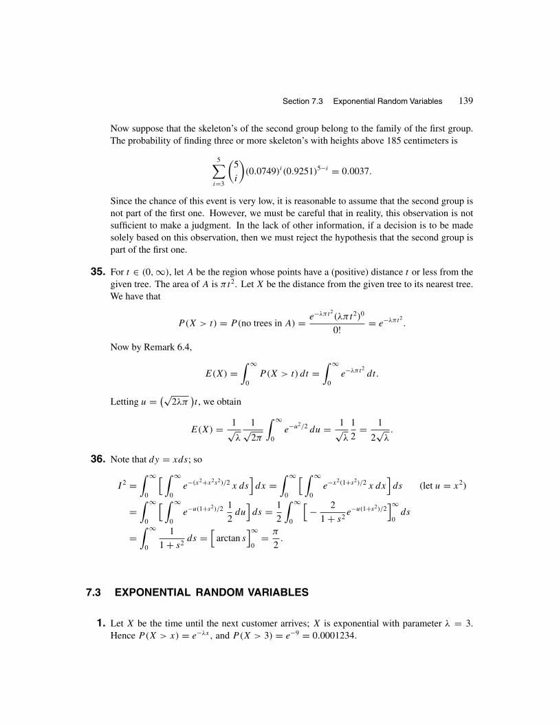
Section 7.3 Exponential Random Variables 139
Now suppose that the skeleton’s of the second group belong to the family of the first group.The probability of finding three or more skeleton’s with heights above 185 centimeters is
5∑i=3
(5
i
)(0.0749)i(0.9251)5−i = 0.0037.
Since the chance of this event is very low, it is reasonable to assume that the second group isnot part of the first one. However, we must be careful that in reality, this observation is notsufficient to make a judgment. In the lack of other information, if a decision is to be madesolely based on this observation, then we must reject the hypothesis that the second group ispart of the first one.
35. For t ∈ (0, ∞), let A be the region whose points have a (positive) distance t or less from thegiven tree. The area of A is πt2. Let X be the distance from the given tree to its nearest tree.We have that
P(X > t) = P(no trees in A) = e−λπt2(λπt2)0
0! = e−λπt2.
Now by Remark 6.4,
E(X) =∫ ∞
0P(X > t) dt =
∫ ∞
0e−λπt2
dt.
Letting u = (√2λπ
)t , we obtain
E(X) = 1√λ
1√2π
∫ ∞
0e−u2/2 du = 1√
λ
1
2= 1
2√
λ.
36. Note that dy = xds; so
I 2 =∫ ∞
0
[ ∫ ∞
0e−(x2+x2s2)/2 x ds
]dx =
∫ ∞
0
[ ∫ ∞
0e−x2(1+s2)/2 x dx
]ds (let u = x2)
=∫ ∞
0
[ ∫ ∞
0e−u(1+s2)/2 1
2du]ds = 1
2
∫ ∞
0
[− 2
1 + s2e−u(1+s2)/2
]∞0
ds
=∫ ∞
0
1
1 + s2ds =
[arctan s
]∞0
= π
2.
7.3 EXPONENTIAL RANDOM VARIABLES
1. Let X be the time until the next customer arrives; X is exponential with parameter λ = 3.Hence P(X > x) = e−λx, and P(X > 3) = e−9 = 0.0001234.

140 Chapter 7 Special Continuous Distributions
2. Let m be the median of an exponential random variable with rate λ. Then P(X > m) = 1/2;
thus e−λm = 1/2 or m = ln 2
λ.
3. For −∞ < y < ∞,
P(Y ≤ y) = P(− ln X ≤ y) = P(X ≥ e−y
) = e−e−y
.
Thus g(y), the probability density function of Y is given by
g(y) = d
dyP (Y ≤ y) = e−y · e−e−y = e−y − e−y
.
4. Let X be the time between the first and second heart attacks. We are given that P(X ≤ 5) =1/2. Since exponential is memoryless, the probability that a person who had one heart attackfive years ago will not have another one during the next five years is still P(X > 5) which is1 − P(X ≤ 5) = 1/2.
5. (a) Suppose that the next customer arrives in X minutes. By the memoryless property, thedesired probability is
P(X <
1
30
)= 1 − e−5(1/30) = 0.1535.
(b) Let Y be the time between the arrival times of the 10th and 11th customers; Y is exponentialwith λ = 5. So the answer is
P(Y ≤ 1
30
)= 1 − e−5(1/30) = 0.1535.
6.
P(|X − E(X)| ≥ 2σX
) = P(∣∣∣X − 1
λ
∣∣∣ ≥ 2
λ
)= P
(X − 1
λ≥ 2
λ
)+ P
(X − 1
λ≤ −2
λ
)= P
(X ≥ 3
λ
)+ P
(X ≤ −1
λ
)= e−λ(3/λ) + 0 = e−3 = 0.049787.
7. (a) P(X > t) = e−λt .
(b) P(t ≤ X ≤ s) = (1 − e−λs
)− (1 − e−λt
) = e−λt − e−λs.
8. The number of documents typed by the secretary on a given eight-hour working day is Poissonwith parameter λ = 8. So the answer is
∞∑i=12
e−88 i
i! = 1 −11∑i=0
e−88 i
i! = 1 − 0.888 = 0.112.

Section 7.3 Exponential Random Variables 141
9. The answer is
E[350 − 40N(12)
] = 350 − 40( 1
18· 12
)= 323.33.
10. Mr. Jones makes his phone calls when either A or B is finished his call. At that time theremaining phone call of A or B, whichever is not finished, and the duration of the call ofMr. Jones both have the same distribution due to the memoryless property of the exponentialdistribution. Hence, by symmetry, the probability that Mr. Jones finishes his call sooner thanthe other one is 1/2.
11. Let N(t) be the number of change-of-states occurring in [0, t]. Let X1 be the time until themachine breaks down for the first time. Let X2 be the time it will take to repair the machine,X3 be the time since the machine was fixed until it breaks down again, and so on. Clearly, X1,X2, . . . are the times between consecutive change of states. Since {X1, X2, . . . } is a sequenceof independent and identically distributed exponential random variables with mean 1/λ, byRemark 7.2,
{N(t) : t ≥ 0
}is a Poisson process with rate λ. Therefore, N(t) is a Poisson
random variable with parameter λt .
12. The probability mass function of L is given by
P(L = n) = (1 − p)n−1p, n = 1, 2, 3, . . . .
HenceP(L > n) = (1 − p)n, n = 0, 1, 2, . . . .
Therefore,
P(T ≤ x) = P(L ≤ 1000x) = 1 − P(L > 1000x) = 1 − (1 − p)1000x
= 1 − e1000x ln(1−p) = 1 − e−x[−1000 ln(1−p)], x > 0.
This shows that T is exponential with parameter λ = −1000 ln(1 − p).
13. (a) We must have∫ ∞
−∞ce−|x| dx = 1; thus
c = 1∫ ∞
−∞e−|x| dx
= 1
2∫ ∞
0e−x dx
= 1
2.
(b) E(X2n+1) =∫ ∞
−∞1
2x2n+1e−|x| dx = 0, because the integrand is an odd function.
E(X2n) =∫ ∞
−∞1
2x2ne−|x| dx =
∫ ∞
0x2ne−x dx,
because the integrand is an even function. We now use induction to prove that∫ ∞
0xne−x dx =
n!. For n = 1, the integral is the expected value of an exponential random variable with

142 Chapter 7 Special Continuous Distributions
parameter 1; so it equals to 1 = 1!. Assume that the identity is valid for n − 1. Usingintegration by parts, we show it for n.∫ ∞
0xne−x dx = −
[− xne−x
]∞0
+∫ ∞
0nxn−1e−x dx = 0 + n(n − 1)! = n!.
Hence E(X2n) = (2n)!.
14. P([X] = n
) = P(n ≤ X < n + 1) =∫ n+1
n
λe−λx dx = −e−λx∣∣∣n+1
n= (
e−λ)n(
1 − e−λ). This
is the probability mass function of a geometric random variable with parameter p = 1 − e−λ.
15. Let that G(t) = P(X > t) = 1 − F(t). By the memoryless property of X,
P(X > s + t | X > t) = P(X > s),
for all s ≥ 0 and t ≥ 0. This implies that
P(X > s + t) = P(X > s)P (X > t),
or
G(s + t) = G(s)G(t), t ≥ 0, s ≥ 0. (24)
Now for arbitrary positive integers n and m, (24) gives that
G(2
n
)= G
(1
n+ 1
n
)= G
(1
n
)G(1
n
)=[G(1
n
)]2,
G(3
n
)= G
(2
n+ 1
n
)= G
(2
n
)G(1
n
)=[G(1
n
)]2G(1
n
)= G
(1
n
)3,
...
G(m
n
)=[G(1
n
)]m
.
Also
G(1) = G
(1
n+ 1
n+ · · · + 1
n︸ ︷︷ ︸n terms
)=[G(1
n
)]n
yields
G(1
n
)= [
G(1)]1/n
. (25)
Hence
G(m/n) = [G(1)
]m/n. (26)

Section 7.3 Exponential Random Variables 143
Now we show that G(1) > 0. If not, G(1) = 0 and by (25), G(1/n) = 0 for all positiveinteger n. This and right continuity of G imply that
P(X ≤ 0) = F(0) = 1 − G(0) = 1 − G(
limn→∞
1
n
)= 1 − lim
n→∞ G(1
n
)= 1 − 0 = 1,
which is a contradiction to the given fact that X is a positive random variable. Thus G(1) > 0and we can define λ = − ln
[G(1)
]. This gives
G(1) = e−λ,
and by (26),G(m/n) = e−λ(m/n).
Thus far, we have proved that for any positive rational t ,
G(t) = e−λt . (27)
To prove the same relation for a positive irrational number t , recall from calculus that for each
positive integer n, there exists a rational number tn in(t, t + 1
n
). Since t < tn < t + 1
n,
limn→∞ tn exists and is t . On the other hand because F is right continuous, G = 1 −F is alsoright continuous and so
G(t) = limn→∞ G(tn).
But since tn is rational, (27) implies that, G(tn) = e−λtn . Hence
G(t) = limn→∞ e−λtn = e−λt .
Thus F(t) = 1 − e−λt for all t , and X is exponential.
Remark: If X is memoryless, then P(X ≤ 0) = 0. To see this, note that P(X > s + t | X >
t) = P(X > s) implies P(X ≤ s + t | X > t) = P(X ≤ s). Letting s = t = 0, we getP(X ≤ 0 | X > 0) = P(X ≤ 0). But P(X ≤ 0 | X > 0) = 0; therefore P(X ≤ 0) = 0.This shows that the memoryless property cannot be defined for random variables possessingnonpositive values with positive probability.
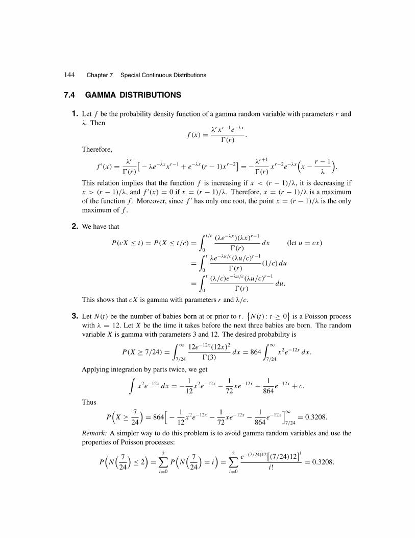
144 Chapter 7 Special Continuous Distributions
7.4 GAMMA DISTRIBUTIONS
1. Let f be the probability density function of a gamma random variable with parameters r andλ. Then
f (x) = λrxr−1e−λx
(r).
Therefore,
f ′(x) = λr
(r)
[− λe−λxxr−1 + e−λx(r − 1)xr−2] = −λr+1
(r)xr−2e−λx
(x − r − 1
λ
).
This relation implies that the function f is increasing if x < (r − 1)/λ, it is decreasing ifx > (r − 1)/λ, and f ′(x) = 0 if x = (r − 1)/λ. Therefore, x = (r − 1)/λ is a maximumof the function f . Moreover, since f ′ has only one root, the point x = (r − 1)/λ is the onlymaximum of f .
2. We have that
P(cX ≤ t) = P(X ≤ t/c) =∫ t/c
0
(λe−λx)(λx)r−1
(r)dx (let u = cx)
=∫ t
0
λe−λu/c(λu/c)r−1
(r)(1/c) du
=∫ t
0
(λ/c)e−λu/c(λu/c)r−1
(r)du.
This shows that cX is gamma with parameters r and λ/c.
3. Let N(t) be the number of babies born at or prior to t .{N(t) : t ≥ 0
}is a Poisson process
with λ = 12. Let X be the time it takes before the next three babies are born. The randomvariable X is gamma with parameters 3 and 12. The desired probability is
P(X ≥ 7/24) =∫ ∞
7/24
12e−12x(12x)2
(3)dx = 864
∫ ∞
7/24x2e−12x dx.
Applying integration by parts twice, we get∫x2e−12x dx = − 1
12x2e−12x − 1
72xe−12x − 1
864e−12x + c.
Thus
P(X ≥ 7
24
)= 864
[− 1
12x2e−12x − 1
72xe−12x − 1
864e−12x
]∞7/24
= 0.3208.
Remark: A simpler way to do this problem is to avoid gamma random variables and use theproperties of Poisson processes:
P(N( 7
24
)≤ 2
)=
2∑i=0
P(N( 7
24
)= i
)=
2∑i=0
e−(7/24)12[(7/24)12
]ii! = 0.3208.

Section 7.4 Gamma Distributions 145
4.
∫ ∞
−∞f (x) dx =
∫ ∞
0
λe−λx(λx)r−1
(r)dx = λr
(r)
∫ ∞
0e−λxxr−1 dx.
Let t = λx; then dt = λdx, so
∫ ∞
−∞f (x) dx = λr
(r)
∫ ∞
0e−t · t r−1
λr−1· 1
λdx
= 1
(r)
∫ ∞
0e−t t r−1 dt = 1
(r) (r) = 1.
5. Let X be the time until the restaurant starts to make profit; X is a gamma random variable withparameters 31 and 12. Thus E(X) = 31/12; that is, two hours and 35 minutes.
6. By the method of Example 5.17, the number of defective light bulbs produced is a Poissonprocess at the rate of (200)(0.015) = 3 per hour. Therefore, X, the time until 25 defectivelight bulbs are produced is gamma with parameters λ = 3 and r = 25. Hence
E(X) = r
λ= 25
3= 8.33.
That is, it will take, on average, 8 hours and 20 minutes to fill up the can.
7.
(1
2
)=∫ ∞
0t−1/2e−t dt.
Making the substitution t = y2/2, we get
(1
2
)= √
2∫ ∞
0e−y2/2 dy =
√2
2
∫ ∞
−∞e−y2/2 dy
= √π · 1√
2π
∫ ∞
−∞e−y2/2 dy = √
π.

146 Chapter 7 Special Continuous Distributions
Hence
(3
2
)= 1
2 (1
2
)= 1
2· √
π,
(5
2
)= 3
2 (3
2
)= 3
2· 1
2· √
π,
(7
2
)= 5
2 (5
2
)= 5
2· 3
2· 1
2· √
π,
...
(n + 1
2
)=
(2n + 1
2
)= 2n − 1
2· 2n − 3
2· · · 7
2· 5
2· 3
2· 1
2· √
π
= (2n)!22n[(2n) · · · 6 · 4 · 2
]√π
= (2n)!√π
2n · 2n · n! = (2n)!√π
4n · n! .
8. (a) Let F be the probability distribution function of Y . For t ≤ 0, F(t) = P(Z2 ≤ t) = 0.For t > 0,
F(t) = P(Y ≤ t) = P(Z2 ≤ t
) = P(− √
t ≤ Z ≤ √t)
= �(√
t)− �
(− √t) = �
(√t)−
[1 − �
(√t)] = 2�
(√t)− 1.
Let f be the probability density function of Y . For t ≤ 0, f (t) = 0. For t > 0,
f (t) = F ′(t) = 2 · 1
2√
t�
′(√t) = 1√
t· 1√
2πe−t/2 = 1√
2πte−t/2 =
1
2e−t/2
(1
2t)−1/2
(1/2),
where by the previous exercise,√
π = (1/2). This shows that Y is gamma with parametersλ = 1/2 and r = 1/2.
(b) Since (X − µ)/σ is standard normal, by part (a), W is gamma with parameters λ = 1/2and r = 1/2.
9. The following solution is an intuitive one. A rigorous mathematical solution would have toconsider the sum of two random variables, each being the minimum of n exponential random
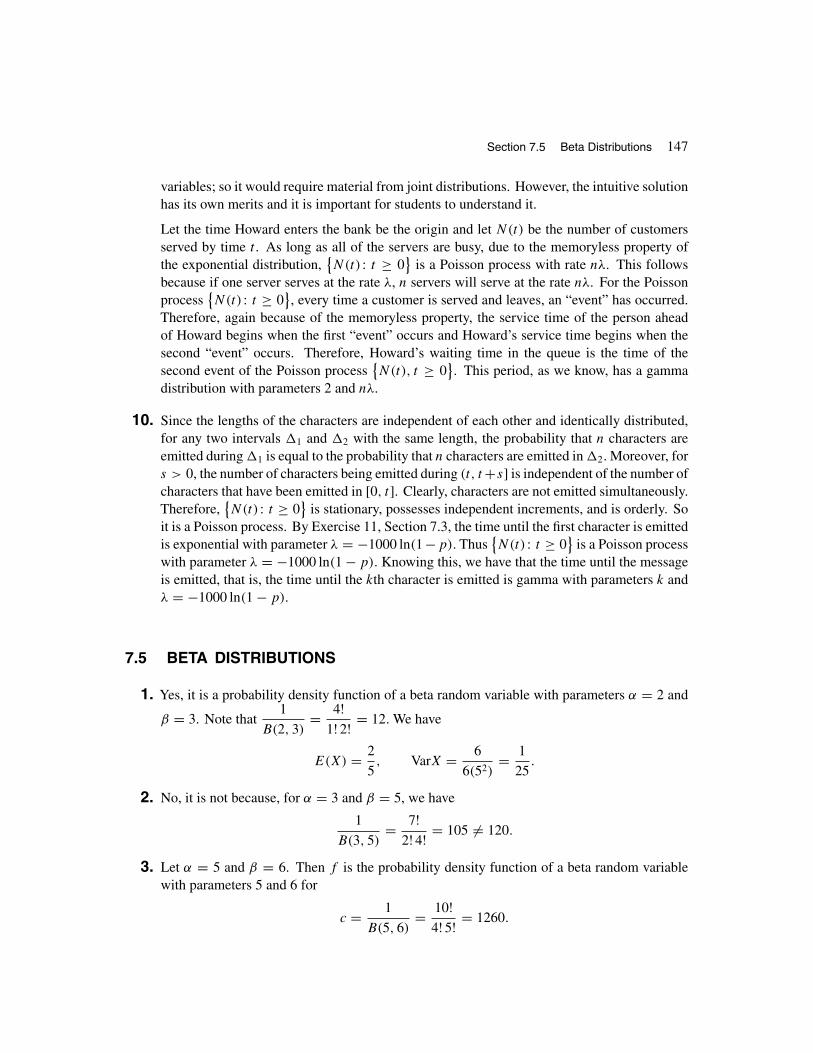
Section 7.5 Beta Distributions 147
variables; so it would require material from joint distributions. However, the intuitive solutionhas its own merits and it is important for students to understand it.
Let the time Howard enters the bank be the origin and let N(t) be the number of customersserved by time t . As long as all of the servers are busy, due to the memoryless property ofthe exponential distribution,
{N(t) : t ≥ 0
}is a Poisson process with rate nλ. This follows
because if one server serves at the rate λ, n servers will serve at the rate nλ. For the Poissonprocess
{N(t) : t ≥ 0
}, every time a customer is served and leaves, an “event” has occurred.
Therefore, again because of the memoryless property, the service time of the person aheadof Howard begins when the first “event” occurs and Howard’s service time begins when thesecond “event” occurs. Therefore, Howard’s waiting time in the queue is the time of thesecond event of the Poisson process
{N(t), t ≥ 0
}. This period, as we know, has a gamma
distribution with parameters 2 and nλ.
10. Since the lengths of the characters are independent of each other and identically distributed,for any two intervals �1 and �2 with the same length, the probability that n characters areemitted during �1 is equal to the probability that n characters are emitted in �2. Moreover, fors > 0, the number of characters being emitted during (t, t +s] is independent of the number ofcharacters that have been emitted in [0, t]. Clearly, characters are not emitted simultaneously.Therefore,
{N(t) : t ≥ 0
}is stationary, possesses independent increments, and is orderly. So
it is a Poisson process. By Exercise 11, Section 7.3, the time until the first character is emittedis exponential with parameter λ = −1000 ln(1−p). Thus
{N(t) : t ≥ 0
}is a Poisson process
with parameter λ = −1000 ln(1 − p). Knowing this, we have that the time until the messageis emitted, that is, the time until the kth character is emitted is gamma with parameters k andλ = −1000 ln(1 − p).
7.5 BETA DISTRIBUTIONS
1. Yes, it is a probability density function of a beta random variable with parameters α = 2 and
β = 3. Note that1
B(2, 3)= 4!
1! 2! = 12. We have
E(X) = 2
5, VarX = 6
6(52)= 1
25.
2. No, it is not because, for α = 3 and β = 5, we have
1
B(3, 5)= 7!
2! 4! = 105 �= 120.
3. Let α = 5 and β = 6. Then f is the probability density function of a beta random variablewith parameters 5 and 6 for
c = 1
B(5, 6)= 10!
4! 5! = 1260.

148 Chapter 7 Special Continuous Distributions
For this value of c,
E(X) = 5
11, VarX = 30
12(112)= 5
242.
4. The answer is
P(p ≥ 0.60) =∫ 1
0.60
1
B(20, 13)x19 (1 − x)12 dx
= 32!19! 12!
∫ 1
0.60x19 (1 − x)12 dx = 0.538.
5. Let X be the proportion of resistors the procurement office purchases from this vendor. Weknow that X is beta. Let α and β be the parameters of the density function of X. Then⎧⎪⎪⎪⎨⎪⎪⎪⎩
α
α + β= 1
3
αβ
(α + β + 1)(α + β)2= 1
18.
Solving this system of 2 equations in 2 unknowns, we obtain α = 1 and β = 2. The desiredprobability is
P(X ≥ 7/12) =∫ 1
7/12
1
B(1, 2)x1−1 (1 − x)2−1 dx = 2
∫ 1
7/12(1 − x) dx = 50
288≈ 0.17.
6. Let X be the median of the fractions for the 13 sections of the course; X is a beta randomvariable with parameters 7 and 7. Let Y be a binomial random variable with parameters 13and 0.40. By Theorem 7.2,
P(X ≤ 0.40) = P(Y ≥ 7).
Therefore,
P(X ≥ 0.40) = P(Y ≤ 6) =6∑
i=0
(13
i
)(0.40)i(0.60)13−i = 0.771156.
7. Let Y be a binomial random variable with parameters 25 and 0.25; by Theorem 7.2,
P(X ≤ 0.25) = P(Y ≥ 5).
Therefore,
P(X ≥ 0.25) = P(Y < 5) =4∑
i=0
(25
i
)(0.25)i(0.75)25−i = 0.214.

Section 7.5 Beta Distributions 149
8. (a) Clearly,
E(Y ) = a + (b − a)E(X) = a + (b − a)α
α + β,
Var(X) = (b − a)2 Var(X) = (b − a)2αβ
(α + β + 1)(α + β)2.
(b) Note that 0 < X < 1 implies that a < Y < b. Let a < t < b; then
P(Y ≤ t) = P(a + (b − a)X ≤ t
) = P(X ≤ t − a
b − a
)=∫ (t−a)/(b−a)
0
1
B(α, β)xα−1 (1 − x)β−1 dx.
Let y = (b − a)x + a; we have
P(Y ≤ t) =∫ t
a
1
B(α, β)
(y − a
b − a
)α−1(1 − y − a
b − a
)β−1 · 1
b − ady
=∫ t
a
1
b − a· 1
B(α, β)
(y − a
b − a
)α−1(b − y
b − a
)β−1dy.
This shows that the probability density function of Y is
f (y) = 1
b − a· 1
B(α, β)
(y − a
b − a
)α−1(b − y
b − a
)β−1, a < y < b.
(c) Note that a = 2, b = 6. Hence
P(Y < 3) =∫ 3
2
1
4· 4!
1! 2!(y − 2
4
)(6 − y
4
)2dy
= 3
64
∫ 3
2(y − 2)(6 − y)2 dy = 3
64· 67
12= 67
256≈ 0.26.
9. Suppose that
f (x) = 1
B(α, β)xα−1(1 − x)β−1, 0 < x < 1,
is symmetric about a point a. Then f (a −x) = f (a +x). That is, for 0 < x < min(a, 1−a),
(a − x)α−1(1 − a + x)β−1 = (a + x)α−1(1 − a − x)β−1. (28)
Since α and β are not necessarily integers, for (a−x)α−1 and (1−a−x)β−1 to be well-defined,we need to restrict ourselves to the range 0 < x < min(a, 1 − a). Now, if a < 1 − a, then,by continuity, (28) is valid for x = a. Substituting a for x in (28), we obtain
(2a)α−1(1 − 2a)β−1 = 0.

150 Chapter 7 Special Continuous Distributions
Since a �= 0, this implies that a = 1/2. If 1 − a < a, then, by continuity, (28) is valid forx = 1 − a. Substituting 1 − a for x in (28), we obtain
(2a − 1)α−1(2 − 2a)β−1 = 0.
Since a �= 1, this implies that a = 1/2. Therefore, in either case a = 1/2. In (28), substitutinga = 1/2, and taking x = 1/4, say, we get
(1/4)α−1(3/4)β−1 = (3/4)α−1(1/4)β−1.
This gives 3β−α = 0, which can only hold for α = β. Therefore, only beta density functionswith α = β are symmetric, and they are symmetric about a = 1/2.
10. t = 0 gives x = 0; t = ∞ gives x = 1. Since dx = 2t
(1 + t2)2dt , we have
B(α, β) =∫ ∞
0
( t2
1 + t2
)α−1( 1
1 + t2
)β−1 · 2t
(1 + t2)2dt = 2
∫ ∞
0t2α−1(1 + t2)−(α+β) dt.
11. We have that
B(α, β) =∫ 1
0xα−1(1 − x)β−1 dx.
Let x = cos2 θ to obtain
B(α, β) = 2∫ π/2
0(cos θ)2α−1(sin θ)2β−1 dθ.
Now
(α) =∫ ∞
0tα−1e−t dt.
Use the substitution t = y2 to obtain
(α) = 2∫ ∞
0y2α−1e−y2
dy.
This implies that
(α) (β) = 4∫ ∞
0
∫ ∞
0x2α−1y2β−1e−(x2+y2) dxdy.
Now we evaluate this double integral by means of a change of variables to polar coordinates:y = r sin θ , x = r cos θ; we obtain
(α) (β) = 4∫ ∞
0
∫ π/2
0r2(α+β)−1(cos θ)2α−1(sin θ)2β−1e−r2
dθdr
= 2B(α, β)
∫ ∞
0r2(α+β)−1e−r2
dr = B(α, β)
∫ ∞
0uα+β−1e−u du (let u = r2)
= B(α, β) (α + β).

Section 7.5 Beta Distributions 151
Thus
B(α, β) = (α) (β)
(α + β).
12. We will show that E(X2) = n/(n − 2). Since E(X2) < ∞, by Remark 6.6, E(X) < ∞.Since E(X) exists and xf (x) is an odd function, we have
E(X) =∫ ∞
−∞xf (x) dx = 0.
Consequently,
Var(X) = E(X2) − [E(X)
]2 = n
n − 2.
Therefore, all we need to find is E(X2). By Theorem 6.3,
E(X2) = (n + 1
2
)√
nπ (n
2
) ∫ ∞
−∞x2(
1 + x2
n
)−(n+1)/2dx.
Substituting x = (√
n )t in this integral yields
E(X2) = (n + 1
2
)√
nπ (n
2
) ∫ ∞
−∞(nt2)(1 + t2)−(n+1)/2 √
n dt
= (n + 1
2
)√
π (n
2
) · 2n
∫ ∞
0t2(1 + t2)−(n+1)/2 dt.
By the previous two exercises,
2∫ ∞
0t2(1 + t2)−(n+1)/2 dt = B
(3
2,n − 2
2
)=
(3
2
) (n − 2
2
) (n + 1
2
) .
Therefore,
E(X2) = (n + 1
2
)√
π · (n
2
) · n · (3
2
) (n − 2
2
) (n + 1
2
) =n (3
2
) (n − 2
2
)√
π (n
2
) .
By the solution to Exercise 7, Section 7.4, (1/2) = √π. Using the identity (r+1) = r (r),
we have
(3
2
)= 1
2 (1
2
)=
√π
2;
(n
2
)=
(n − 2
2+ 1
)= n − 2
2 (n − 2
2
).

152 Chapter 7 Special Continuous Distributions
Consequently,
E(X2) =n
√π
2 (n − 2
2
)√
π · n − 2
2 (n − 2
2
) = n
n − 2.
7.6 SURVIVAL ANALYSIS AND HAZARD FUNCTIONS
1. Let X be the lifetime of the electrical component, F be its probability distribution function,and λ(t) be its failure rate. For some constants α and β, we are given that
λ(t) = αt + β.
Since λ(48) = 0.10 and λ(72) = 0.15,{48α + β = 0.10
72α + β = 0.15.
Solving this system of two equations in two unknowns gives α = 1/480 and β = 0. Henceλ(t) = t/480. By (7.6), for t > 0,
P(X > t) = F (t) = exp(−∫ t
0
u
480du)
= e−t2/960.
Let f be the probability density function of X. This also gives
f (t) = − d
dtF (t) = t
480e−t2/960.
The answer to part (a) is
P(X > 30) = e−900/960 = e−0.9375 = 0.392.
The exact value for part (b) is
P(X < 31 | X > 30) = P(30 < X < 31)
P (X > 30)
= 1
0.392
∫ 31
30(t/480)e−t2/960 dt = 0.02411
0.392= 0.0615.
Note that for small �t , λ(t)�t is approximately the probability that the component failswithin �t hours after t , given that it has not yet failed by time t . Letting �t = 1, for t = 30,λ(t)�t ≈ 0.0625 which is relatively close to the exact value of 0.0615. This is interestingbecause �t = 1 is not that small, and one may not expect close approximations anyway.

Chapter 7 Review Problems 153
2. Let F be the survival function of a Weibull random variable. We have
F (t) =∫ ∞
t
αxα−1e−xα
dx.
Letting u = xα, we have du = αxα−1 dx. Thus
F (t) =∫ ∞
tαe−u du = −e−u
∣∣∣∞tα
= e−tα .
Therefore,
λ(t) = αtα−1e−tα
e−tα= αtα−1·
λ(t) = 1, for α = 1; so the Weibull in this case is exponential with parameter 1. Clearly, forα < 1, λ′(t) < 0; so λ(t) is decreasing. For α > 1, λ′(t) > 0; so λ(t) is increasing. Note thatfor α = 2, the failure rate is the straight line λ(t) = 2t.
REVIEW PROBLEMS FOR CHAPTER 7
1.30 − 25
37 − 25= 5
12.
2. Let X be the weight of a randomly selected women from this community. The desired quantityis
P(X > 170 | X > 140) = P(X > 170)
P (X > 140)=
P(Z >
170 − 130
20
)P(Z >
140 − 130
20
)= P(Z > 2)
P (Z > 0.5)= 1 − �(2)
1 − �(0.5)= 1 − 0.9772
1 − 0.6915= 0.074.
3. Let X be the number of times the digit 5 is generated; X is binomial with parameters n = 1000and p = 1/10.Thus np = 100 and
√np(1 − p) = √
90 = 9.49. Using normal approximationand making correction for continuity,
P(X ≤ 93.5) = P(Z ≤ 93.5 − 100
9.49
)= P(Z ≤ −0.68) = 1 − �(0.68) = 0.248.
4. The given relation implies that
1 − e−2λ = 2[(1 − e−3λ) − (1 − e−2λ)
].

154 Chapter 7 Special Continuous Distributions
This is equivalent to3e−2λ − 2e−3λ − 1 = 0,
or, equivalently, (e−λ − 1
)2(2e−λ + 1
) = 0.
The only root of this equation is λ = 0 which is not acceptable. Therefore, it is not possiblethat X satisfy the given relation.
5. Let X be the lifetime of a random light bulb. Then
P(X < 1700) = 1 − e−(1/1700)·1700 = 1 − e−1.
The desired probability is
1 − P(none fails) − P(one fails)
= 1 −(
20
0
)(1 − e−1)0(e−1)20 −
(20
1
)(1 − e−1
)(e−1
)19 = 0.999999927.
6. Note that limx→0 x ln x = 0; so
E(− ln X) =∫ 1
0(− ln x) dx =
[x − x ln x
]1
0= 1.
7. Let X be the diameter of the randomly chosen disk in inches. We are given that X ∼ N(4, 1).We want to find the distribution function of 2.5X; we have
P(2.5X ≤ x) = P(X ≤ x/2.5) = 1√2π
∫ x/2.5
−∞e−(t−4)2/2 dt.
8. If α < 0, then α + β < β; therefore,
P(α ≤ X ≤ α + β) = P(0 ≤ X ≤ α + β) ≤ P(0 ≤ X ≤ β).
If α > 0, then e−λα < 1. Thus
P(α ≤ X ≤ α + β) = [1 − e−λ(α+β)
]− (1 − e−λα
)= e−λα
(1 − e−λβ
)< 1 − e−λβ = P(0 ≤ X ≤ β).
9. We are given that 1/λ = 1.25; so λ = 0.8. Let X be the time it takes for a random student tocomplete the test. Since P(X > 1) = e−(0.8)1 = e−0.8, the desired probability is
1 − (e−0.8
)10 = 1 − e−8 = 0.99966.

Chapter 7 Review Problems 155
10. Note thatf (x) = ke−[x−(3/2)]2+17/4 = ke17/4 · e−[x−(3/2)]2
.
Comparing this with the probability density function of a normal random variable with mean3/2, we see that σ 2 = 1/2 and ke17/4 = 1/(σ
√2π). Therefore,
k = 1
σ√
2πe−17/4 = 1
πe−17/4.
11. Let X be the grade of a randomly selected student.
P(X ≥ 90) = P(Z ≥ 90 − 72
7
)= 1 − �(2.57) = 0.0051.
Similarly,
P(80 ≤ X < 90) = P(1.14 ≤ Z < 2.57) = 0.122,
P (70 ≤ X < 80) = P(−0.29 ≤ Z < 1.14) = 0.487,
P (60 ≤ X < 70) = P(−1.71 ≤ Z < −0.29) = 0.3423,
P (X < 60) = P(Z < −1.71) = 0.0436.
Therefore, approximately 0.51% will get A, 12.2% will get B, 48.7% will get C, 34.23% D,and 4.36% F.
12. Since E(X) = 1/λ,
P(X > E(X)
) = e−λ(1/λ) = e−1 = 0.36788.
13. Round off error to the nearest integer is uniform over (−0.5, 0.5); round off error to the nearest1st decimal place is uniform over (−0.05, 0.05); round off error to the nearest 2nd decimalplace is uniform over (−0.005, 0.005), and so on. In general, round off error to the nearest k
decimal places is uniform over (−5/10k+1, 5/10k+1).
14. We want to find the smallest a for which P(X ≤ a) ≥ 0.90. This implies
P(Z ≤ a − 175
22
)≥ 0.90.
Using Table 1 of the appendix, we see that (a − 175)/22 = 1.29 or a = 203.38.
15. Let X be the breaking strength of the yarn under consideration. Clearly,
P(X ≥ 100) = P(Z ≥ 100 − 95
11
)= 1 − �(0.45) = 0.33.
So the desired probability is
1 −(
10
0
)(0.33)0(0.67)10 −
(10
1
)(0.33)1(0.67)9 = 0.89.

156 Chapter 7 Special Continuous Distributions
16. Let X be the time until the 91st call is received. X is a gamma random variable with parametersr = 91 and λ = 23. The desired probability is
P(X ≥ 4) =∫ ∞
4
23e−23x (23x)91−1
(91)dx
= 1 −∫ 4
0
23e−23x (23x)91−1
90! dx
= 1 − 2391
90!∫ 4
0x90e−23x dx = 1 − 0.55542 = 0.44458.
17. Clearly,
E(X) = (1 − θ) + (1 + θ)
2= 1,
Var(X) = (1 + θ − 1 + θ)2
12= θ2
3.
Now
E(X2)− [
E(X)]2 = θ2
3implies that
E(X2) = θ2
3+ 1,
which yeilds 3E(X2)− 1 = θ2, or, equivalently, E(3X2 − 1) = θ2. Therefore, one choice forg(X) is g(X) = 3X2 − 1.
18. Let α and β be the parameters of the density function of X/�. Solving the following twoequations in two unknowns,
E(X/�) = α
α + β= 3
7,
Var(X/�) = αβ
(α + β + 1)(α + β)2= 3
98,
we obtain α = 3 and β = 4. Therefore, X/� is beta with parameters 3 and 4. The desiredprobability is
P(�/7 < X < �/3) = P(1/7 < X/� < 1/3) =∫ 1/3
1/7
1
B(3, 4)x2(1 − x)3 dx
= 60∫ 1/3
1/7x2(1 − x)3 dx = 0.278.

Chapter 8
Bivariate Distributions
8.1 JOINT DISTRIBUTIONS OF TWO RANDOM VARIABLES
1. (a)∑2
x=1
∑2y=1 k(x/y) = 1 implies that k = 2/9.
(b) pX(x) = ∑2y=1
[(2x)/(9y)
] = x/3, x = 1, 2.
pY (y) = ∑2x=1
[(2x)/(9y)
] = 2/(3y), y = 1, 2.
(c) P(X > 1 | Y = 1) = p(2, 1)
pY (1)= 4/9
2/3= 2
3.
(d) E(X) =2∑
y=1
2∑x=1
x · 2
9
(x
y
)= 5
3; E(Y ) =
2∑y=1
2∑x=1
y · 2
9
(x
y
)= 4
3.
2. (a)∑3
x=1
∑2y=1 c(x + y) = 1 implies that c = 1/21.
(b) pX(x) = ∑2y=1(1/21)(x + y) = (2x + 3)/21. x = 1, 2, 3.
pY (y) = ∑3x=1(1/21)(x + y) = (6 + 3y)/21. y = 1, 2.
(c) P(X ≥ 2 | Y = 1) = p(2, 1) + p(3, 1)
pY (1)= 7/21
9/21= 7
9.
(d) E(X) =3∑
x=1
2∑y=1
1
21x(x + y) = 46
21; E(Y ) =
3∑x=1
2∑y=1
1
21y(x + y) = 11
7.
3. (a) k(1 + 1 + 1 + 9 + 4 + 9) = 1 implies that k = 1/25.
(b) pX(1) = p(1, 1) + p(1, 3) = 12/25, pX(2) = p(2, 3) = 13/25;pY (1) = p(1, 1) = 2/25, pY (3) = p(1, 3) + p(2, 3) = 23/25.

158 Chapter 8 Bivariate Distributions
Therefore,
pX(x) =⎧⎨⎩12/25 if x = 1
13/25 if x = 2,pY (y) =
⎧⎨⎩2/25 if y = 1
23/25 if y = 3.
(c) E(X) = 1 · 12
25+ 2 · 13
25= 38
25; E(Y ) = 1 · 2
25+ 3 · 23
25= 71
25.
4. P(X > Y) = p(1, 0) + p(2, 0) + p(2, 1) = 2/5,
P (X + Y ≤ 2) = p(1, 0) + p(1, 1) + p(2, 0) = 7/25,
P (X + Y = 2) = p(1, 1) + p(2, 0) = 6/25.
5. Let X be the number of sheep stolen; let Y be the number of goats stolen. Let p(x, y) be thejoint probability mass function of X and Y . Then, for 0 ≤ x ≤ 4, 0 ≤ y ≤ 4, 0 ≤ x + y ≤ 4,
p(x, y) =
(7
x
)(8
y
)(5
4 − x − y
)(
20
4
) ;
p(x, y) = 0, for other values of x and y.
6. The following table gives p(x, y), the joint probability mass function of X and Y ; pX(x), themarginal probability mass function of X; and pY (y), the marginal probability mass functionof Y .
y
x 0 1 2 3 4 5 pX(x)
2 1/36 0 0 0 0 0 1/363 0 2/36 0 0 0 0 2/364 1/36 0 2/36 0 0 0 3/365 0 2/36 0 2/36 0 0 4/366 1/36 0 2/36 0 2/36 0 5/367 0 2/36 0 2/36 0 2/36 6/368 1/36 0 2/36 0 2/36 0 5/369 0 2/36 0 2/36 0 0 4/3610 1/36 0 2/36 0 0 0 3/3611 0 2/36 0 0 0 0 2/3612 1/36 0 0 0 0 0 1/36
pY (y) 6/36 10/36 8/36 6/36 4/36 2/36
7. p(1, 1) = 0, p(1, 0) = 0.30, p(0, 1) = 0.50, p(0, 0) = 0.20.

Section 8.1 Joint Distributions of Two Random Variables 159
8. (a) For 0 ≤ x ≤ 7, 0 ≤ y ≤ 7, 0 ≤ x + y ≤ 7,
p(x, y) =
(13
x
)(13
y
)(26
7 − x − y
)(
52
7
) .
For all other values of x and y, p(x, y) = 0.
(b) P(X ≥ Y ) = ∑3y=0
∑7−yx=y p(x, y) = 0.61107.
9. (a) fX(x) =∫ x
02 dy = 2x, 0 ≤ x ≤ 1; fY (y) =
∫ 1
y
2 dx = 2(1 − y), 0 ≤ y ≤ 1.
(b) E(X) =∫ 1
0xfX(x) dx =
∫ 1
0x(2x) dx = 2/3;
E(Y ) =∫ 1
0yfY (y) dy =
∫ 1
02y(1 − y) dy = 1/3.
(c) P(X <
1
2
)=∫ 1/2
0fX(x) dx =
∫ 1/2
02x dx = 1
4,
P (X < 2Y ) =∫ 1
0
∫ x
x/22 dy dx = 1
2,
P (X = Y ) = 0.
10. (a) fX(x) =∫ x
08xy dy = 4x3, 0 ≤ x ≤ 1,
fY (y) =∫ 1
y
8xy dx = 4y(1 − y2), 0 ≤ y ≤ 1.
(b) E(X) =∫ 1
0xfX(x) dx =
∫ 1
0x · 4x3 dx = 4/5;
E(Y ) =∫ 1
0yfY (y) dy =
∫ 1
0y · 4y(1 − y2) dy = 8/15.
11. fX(x) =∫ 2
0
1
2ye−x dy = e−x, x > 0; fY (y) =
∫ ∞
0
1
2ye−x dx = 1
2y, 0 < y < 2.
12. Let R = {(x, y) : 0 ≤ x ≤ 1, 0 ≤ y ≤ 1
}. Since area(R) = 1, P(X + Y ≤ 1/2) is the area
of the region{(x, y) ∈ R : x + y ≤ 1/2
}which is 1/8. Similarly, P(X − Y ≤ 1/2) is the

160 Chapter 8 Bivariate Distributions
area of the region{(x, y) ∈ R : x − y ≤ 1/2
}which is 7/8. P(X2 + Y 2 ≤ 1) is the area of
the region{(x, y) ∈ R : x2 + y2 ≤ 1
}which is π/4. P(XY ≤ 1/4) is the sum of the area
of the region{(x, y) : 0 ≤ x ≤ 1/4, 0 ≤ y ≤ 1
}which is 1/4 and the area of the region under
the curve y = 1/(4x) from 1/4 to 1. (Draw a figure.) Therefore,
P(XY ≤ 1/4) = 1
4+∫ 1
1/4
1
4xdx ≈ 0.597.
13. (a) The area of R is∫ 1
0(x − x2) dx = 1
6; so
f (x, y) ={
6 if (x, y) ∈ R
0 elsewhere.
(b) fX(x) =∫ x
x2f (x, y) dy =
∫ x
x26 dy = 6x(1 − x), 0 < x < 1;
fY (y) =∫ √
y
y
f (x, y) dx =∫ √
y
y
6 dx = 6(√
y − y), 0 < y < 1.
(c) E(X) =∫ 1
0xfX(x) dx =
∫ 1
06x2(1 − x) dx = 1/2;
E(Y ) =∫ 1
0yfY (y) dy =
∫ 1
06y(
√y − y) dy = 2/5.
14. Let X and Y be the minutes past 11:30 A.M. that the man and his fiancée arrive at thelobby, respectively. We have that X and Y are uniformly distributed over (0, 30). LetS = {
(x, y) : 0 ≤ x ≤ 30, 0 ≤ y ≤ 30}, and R = {
(x, y) ∈ S : y ≤ x − 12 or y ≥ x + 12}.
The desired probability is the area of R divided by the area of S: 324/900 = 0.36. (Draw afigure.)
15. Let X and Y be two randomly selected points from the interval (0, �). We are interested inE(|X − Y |). Since the joint probability density function of X and Y is
f (x, y) =
⎧⎪⎨⎪⎩1
� 20 < x < �, 0 < y < �
0 elsewhere,

Section 8.1 Joint Distributions of Two Random Variables 161
E(|X − Y |) =
∫ �
0
∫ �
0|x − y| 1
� 2dx dy
= 1
� 2
∫ �
0
[ ∫ y
0(y − x) dx
]dy + 1
� 2
∫ �
0
[ ∫ �
y
(x − y) dx]dy
= �
6+ �
6= �
3.
16. The problem is equivalent to the following: Two random numbers X and Y are selected atrandom and independently from (0, �). What is the probability that |X − Y | < X? LetS = {
(x, y) : 0 < x < �, 0 < y < �}
and
R = {(x, y) ∈ S : |x − y| < x
} = {(x, y) ∈ S : y < 2x
}.
The desired probability is the area of R which is 3� 2/4 divided by � 2. So the answer is 3/4.(Draw a figure.)
17. Let S = {(x, y) : 0 < x < 1, 0 < y < 1
}and R = {
(x, y) ∈ S : y ≤ x and x2 + y2 ≤ 1}.
The desired probability is the area of R which is π/8 divided by the area of S which is 1. Sothe answer is π/8.
18. We prove this for the case in which X and Y are continuous random variables with jointprobability density function f . For discrete random variables the proof is similar. The relationP(X ≤ Y ) = 1, implies that f (x, y) = 0 if x > y. Hence by Theorem 8.2,
E(X) =∫ ∞
−∞
∫ ∞
−∞xf (x, y) dx dy
=∫ ∞
−∞
∫ y
−∞xf (x, y) dx dy
≤∫ ∞
−∞
∫ y
−∞yf (x, y) dx dy
=∫ ∞
−∞
∫ ∞
−∞yf (x, y) dx dy = E(Y ).
19. Let H be the distribution function of a random variable with probability density function h.
That is, let H(x) =∫ x
−∞h(y) dy. Then
P(X ≥ Y ) =∫ ∞
−∞
∫ x
−∞h(x)h(y) dy dx =
∫ ∞
−∞h(x)
[ ∫ x
−∞h(y) dy
]dx
=∫ ∞
−∞h(x)H(x) dx = 1
2
[H(x)
]2∣∣∣∣∞−∞
= 1
2(12 − 02) = 1
2.
20. Since 0 ≤ 2G(x) − 1 ≤ 1, 0 ≤ 2H(y) − 1 ≤ 1, and −1 ≤ α ≤ 1, we have that
−1 ≤ α[2G(x) − 1
][2H(y) − 1
] ≤ 1.
162 Chapter 8 Bivariate Distributions
So0 ≤ 1 + α
[2G(x) − 1
][2H(y) − 1
] ≤ 2.
This and g(x) ≥ 0, h(y) ≥ 0 imply that f (x, y) ≥ 0. To prove that f is a joint probability
density function, it remains to show that∫ ∞
−∞
∫ ∞
−∞f (x, y) dx dy = 1.∫ ∞
−∞
∫ ∞
−∞f (x, y) dx dy
=∫ ∞
−∞
∫ ∞
−∞g(x)h(y) dx dy + α
∫ ∞
−∞
∫ ∞
−∞g(x)h(y)
[2G(x) − 1
][2H(y) − 1
]dx dy
= 1 + α{ ∫ ∞
−∞h(y)
[2H(y) − 1
]dy}{ ∫ ∞
−∞g(x)
[2G(x) − 1
]dx}
= 1 + α1
4
[2H(y) − 1
]2∣∣∣∞−∞
1
4
[2G(x) − 1
]2∣∣∣∞−∞
= 1 + α · 0 · 0 = 1.
Now we calculate the marginals.
fX(x) =∫ ∞
−∞g(x)h(y)
{1 + α
[2G(x) − 1
][2H(y) − 1
]}dy
=∫ ∞
−∞g(x)h(y) dy + α
∫ ∞
−∞g(x)h(y)
[2G(x) − 1
][2H(y) − 1
]dy
= g(x)
∫ ∞
−∞h(y) dy + αg(x)
[2G(x) − 1
] ∫ ∞
−∞h(y)
[2H(y) − 1
]dy
= g(x) + αg(x)[2G(x) − 1
]1
4
[2H(y) − 1
]2∣∣∣∞−∞
= g(x) + αg(x)[2G(x) − 1
] · 0 = g(x) + 0 = g(x).
Similarly, fY (y) = h(y).
21. Orient the circle counterclockwise and let X be the length of the arc NM and Y be length ofthe arc NL. Let R be the radius of the circle; clearly, 0 ≤ X ≤ 2πR and 0 ≤ Y ≤ 2πR.The angle MNL is acute if and only if |Y − X| < πR. Therefore, the sample space of thisexperiment is
S = {(x, y) : 0 ≤ x ≤ 2πR, 0 ≤ y ≤ 2πR
}and the desired event is
E = {(x, y) ∈ S : |y − x| < πR
}.
The probability that � MNL is acute is the area of E which is 3π2R2 divided by the area of S
which is 4π2R2; that is, 3/4.
22. Let
S = {(x, y) ∈ R2 : 0 ≤ x ≤ 1, 0 ≤ y ≤ 1
}, A = {
(x, y) ∈ S : 0 < x + y < 0.5},
B = {(x, y) ∈ S : 0.5 < x + y < 1.5
}, C = {
(x, y) ∈ S : x + y > 1.5}.
Section 8.1 Joint Distributions of Two Random Variables 163
The probability that the integer nearest to x + y is 0 isarea(A)
area (S)= 1
8, The probability that the
integer nearest to x + y is 1 isarea(B)
area(S)= 3
4, and the probability that the nearest integer to
x + y is 2 isarea (C)
area(S)= 1
8.
23. Let X be a random number from (0, a) and Y be a random number from (0, b). In
(4
3
)= 4
ways we can select three of X, a − X, Y , and b − Y . If X, a − X, and Y are selected, atriangular pen is possible to make if and only if X < (a − X) + Y , a − X < X + Y , andY < X + (a − X). The probability of this event is the area of{
(x, y) ∈ R2 : 0 < x < a, 0 < y < b, 2x − y < a, 2x + y > a, y < a}
which is a2/2 divided by the area of
S = {(x, y) ∈ R2 : 0 < x < a, 0 < y < b
}which is ab: (a2/2)/ab = a/(2b). Similarly, for each of the other three 3-combinations ofX, a − x, Y , and b − Y also the probability that the three segments can be used to form atriangular pen is a/(2b). Thus the desired probability is
1
4· a
2b+ 1
4· a
2b+ 1
4· a
2b+ 1
4· a
2b= a
2b.
24. Let X and Y be the two points that are placed on the segment. Let E be the event that the lengthof none of the three parts exceeds the given value α. Clearly, P(E | X < Y) = P(E | Y < X)
and P(X < Y) = P(Y < X) = 1/2. Therefore,
P(E) = P(E | X < Y)P (X < Y) + P(E | Y < X)P (Y < X)
= P(E | X < Y)1
2+ P(E | X < Y)
1
2= P(E | X < Y).
This shows that for calculation of P(E), we may reduce the sample space to the case whereX < Y . The reduced sample space is
S = {(x, y) : x < y, 0 < x < �, 0 < y < �
}.
The desired probability is the area of
R = {(x, y) ∈ S : x < α, y − x < α, y > � − α
}divided by area(S) = � 2/2. But
area(R) =
⎧⎪⎪⎪⎨⎪⎪⎪⎩(3α − �)2
2if
�
3≤ α ≤ �
2� 2
2− 3� 2
2
(1 − α
�
)2if
�
2≤ α ≤ �.
164 Chapter 8 Bivariate Distributions
Hence the desired probability is
P(E) =
⎧⎪⎪⎨⎪⎪⎩(3α
�− 1
)2if
�
3≤ α ≤ �
2
1 − 3(
1 − α
�
)2if
�
2≤ α ≤ �.
25. R is the square bounded by the lines x + y = 1, −x + y = 1, −x − y = 1, and x − y = 1; itsarea is 2. To find the probability density function of X, the x-coordinate of the point selectedat random from R, first we calculate P(X ≤ t), ∀t . For −1 ≤ t < 0, P(X ≤ t) is the area ofthe triangle bound by the lines −x + y = 1, −x − y = 1, and x = t which is (1 + t)2 dividedby area(R) = 2. (Draw a figure.) For 0 ≤ t < 1, P(X ≤ t) is the area inside R to the left ofthe line x = t which is 2 − (1 − t)2 divided by area(R) = 2. Therefore,
P(X ≤ t) =
⎧⎪⎪⎪⎪⎪⎪⎪⎪⎪⎨⎪⎪⎪⎪⎪⎪⎪⎪⎪⎩
0 t < −1
(1 + t)2
2−1 ≤ t < 0
2 − (1 − t)2
20 ≤ t < 1
1 t ≥ 1,
and hence
d
dtP (X ≤ t) =
⎧⎪⎨⎪⎩1 + t −1 ≤ t < 0
1 − t 0 ≤ t < 1
0 otherwise.
This shows that fX(t), the probability density function of X is given by fX(t) = 1 − |t |,−1 ≤ t ≤ 1; 0, elsewhere.
26. Clearly,
P(Z ≤ z) =∫∫
{(x,y) : y/x≤z}f (x, y) dx dy.
Now for x > 0, y/x ≤ z if and only if y ≤ xz; for x < 0, y/x ≤ z if and only if y ≥ xz.Therefore, integration region is{
(x, y) : x < 0, y ≥ xz} ∪ {(x, y) : x > 0, y ≤ xz
}.
Thus
P(Z ≤ z) =∫ 0
−∞
( ∫ ∞
xz
f (x, y) dy)
dx +∫ ∞
0
( ∫ xz
−∞f (x, y) dy
)dx.

Section 8.1 Joint Distributions of Two Random Variables 165
Using the substitution y = tx, we get
P(Z ≤ z) =∫ 0
−∞
( ∫ −∞
z
xf (x, tx) dt)
dx +∫ ∞
0
( ∫ z
−∞xf (x, tx) dt
)dx
=∫ 0
−∞
( ∫ z
−∞−xf (x, tx) dt
)dx +
∫ ∞
0
( ∫ z
−∞xf (x, tx) dt
)dx
=∫ 0
−∞
( ∫ z
−∞|x|f (x, tx) dt
)dx +
∫ ∞
0
( ∫ z
−∞|x|f (x, tx) du
)dx
=∫ ∞
−∞
( ∫ z
−∞|x|f (x, tx) dt
)dx =
∫ z
−∞
( ∫ ∞
−∞|x|f (x, tx) dx
)dt.
Differentiating with respect to z, Fundamental Theorem of Calculus implies that,
fZ(z) = d
dzP (Z ≤ z) =
∫ ∞
−∞|x|f (x, xz) dx.
27. Note that there are exactly n such closed semicircular disks because the probability that thediameter through Pi contains any other point Pj is 0. (Draw a figure.) Let E be the event thatall the points are contained in a closed semicircular disk. Let Ei be the event that the pointsare all in Di . Clearly, E = ∪n
i=1Ei . Since there is at most one Di , 1 ≤ i ≤ n, that contains allthe Pi’s, the events E1, E2, . . . , En are mutually exclusive. Hence
P(E) = P( n⋃
i=1
Ei
)=
n∑i=1
P(Ei) =n∑
i=1
(1
2
)n−1 = n(1
2
)n−1,
where the next-to-the-last equality follows because P(Ei) is the probability that P1, P2,. . . , Pi−1, Pi+1, . . . , Pn fall inside Di . The probability that any of these falls inside Di is(area of Di)/(area of the disk) = 1/2 independently of the others. Hence the probability thatall of them fall inside Di is (1/2)n−1.
28. We have that
fX(x) = (α + β + γ )
(α) (β) (γ )
∫ 1−x
0xα−1yβ−1(1 − x − y)γ−1 dy
= 1
B(α, β + γ )B(β, γ )xα−1
∫ 1−x
0yβ−1(1 − x − y)γ−1 dy.
Let z = y/(1 − x); then dy = (1 − x) dz, and∫ 1−x
0yβ−1(1−x −y)γ−1 dy = (1−x)β+γ−1
∫ 1
0zβ−1(1− z)γ−1 dz = (1−x)β+γ−1B(β, γ ).
So
fX(x) = 1
B(α, β + γ )B(β, γ )xα−1(1 − x)β+γ−1B(β, γ )
= 1
B(α, β + γ )xα−1(1 − x)β+γ−1.

166 Chapter 8 Bivariate Distributions
This shows that X is beta with parameters (α, β + γ ). A similar argument shows that Y isbeta with parameters (β, γ + α).
29. It is straightforward to check that f (x, y) ≥ 0, f is continuous and∫ ∞
−∞
∫ ∞
−∞f (x, y) dx dy = 1.
Therefore, f is a continuous probability density function. We will show that∂F
∂xdoes not
exist at (0, 0). Similarly, one can show that∂F
∂xdoes not exist at any point on the y-axis. Note
that for small �x > 0,
F(�x, 0) − F(0, 0) = P(X ≤ �x , Y ≤ 0) − P(X ≤ 0 , Y ≤ 0)
= P(0 ≤ X ≤ �x , Y ≤ 0) =∫ 0
−∞
∫ �x
0f (x, y) dx dy.
Now, from the definition of f (x, y), we must have �x < (1/2)ey or, equivalently,y > ln(2�x). Thus, for small �x > 0,
F(�x, 0) − F(0, 0) =∫ 0
ln(2�x)
∫ �x
0(1 − 2xe−y) dx dy = (�x)2 −
[(�x) ln(2�x) + �x
2
].
This implies that
lim�x→0+
F(�x, 0) − F(0, 0)
�x= lim
�x→0+
[�x − ln(2�x) − 1
2
]= ∞,
showing that∂F
∂xdoes not exist at (0, 0).
8.2 INDEPENDENT RANDOM VARIABLES
1. Note that pX(x) = (1/25)(3x2 + 5), pY (y) = (1/25)(2y2 + 5). Now pX(1) = 8/25,pY (0) = 5/25, and p(1, 0) = 1/25. Since p(1, 0) �= pX(1)pY (0), X and Y are dependent.
2. Note that
p(1, 1) = 1
7,
pX(1) = p(1, 1) + p(1, 2) = 1
7+ 2
7= 3
7,
pY (1) = p(1, 1) + p(2, 1) = 1
7+ 5
7= 6
7.
Since p(1, 1) �= pX(1)pY (1), X and Y are dependent.

Section 8.2 Independent Random Variables 167
3. By the independence of X and Y ,
P(X = 1, Y = 3) = P(X = 1)P (Y = 3) = 1
2
(2
3
)· 1
2
(2
3
)3 = 4
81.
P (X + Y = 3) = P(X = 1, Y = 2) + P(X = 2, Y = 1)
= 1
2
(2
3
)· 1
2
(2
3
)2 + 1
2
(2
3
)2 · 1
2
(2
3
)= 4
27.
4. No, they are not independent because, for example, P(X = 0 | Y = 8) = 1 but
P(X = 0) =
(39
8
)(
52
8
) = 0.08175 �= 1,
showing that P(X = 0 | Y = 8) �= P(X = 0).
5. The answer is (7
2
)(1
2
)2(1
2
)5 ·(
8
2
)(1
2
)2(1
2
)6 = 0.0179.
6. We have that
P(
max(X, Y ) ≤ t) = P(X ≤ t, Y ≤ t) = P(X ≤ t)P (Y ≤ t) = F(t)G(t).
P(
min(X, Y ) ≤ t) = 1 − P
(min(X, Y ) > t
)= 1 − P(X > t, Y > t) = 1 − P(X > t)P (Y > t)
= 1 − [1 − F(t)
][1 − G(t)
] = F(t) + G(t) − F(t)G(t).
7. Let X and Y be the number of heads obtained by Adam and Andrew, respectively. The desiredprobability is
n∑i=0
P(X = i, Y = i) =n∑
i=0
P(X = i)P (Y = i)
=n∑
i=0
(n
i
)(1
2
)i(1
2
)n−i ·(
n
i
)(1
2
)i(1
2
)n−i
=(1
2
)2nn∑
i=0
(n
i
)2
=(1
2
)2n(
2n
n
),
where the last equality follows by Example 2.28.

168 Chapter 8 Bivariate Distributions
An Intuitive Solution: Let Z be the number of tails obtained by Andrew. The desired proba-bility is
n∑i=0
P(X = i, Y = i) =n∑
i=0
P(X = i, Z = i) =n∑
i=0
P(X = i, Y = n − i)
= P(Adam and Andrew get a total of n heads)
= P( n heads in 2n flips of a fair coin) =(1
2
)2n(
2n
n
).
8. For i, j ∈ {0, 1, 2, 3
}, the sum of the numbers in the ith row is pX(i) and the sum of the
numbers in the j th row is pY (j). We have that
pX(0) = 0.41, pX(1) = 0.44, pX(2) = 0.14, pX(3) = 0.01;pY (0) = 0.41, pY (1) = 0.44, pY (2) = 0.14, pY (3) = 0.01.
Since for all x, y ∈ {0, 1, 2, 3}, p(x, y) = pX(x)pY (y), X and Y are independent.
9. They are not independent because
fX(x) =∫ x
02 dy = 2x, 0 ≤ x ≤ 1;
fY (y) =∫ 1
y
2 dx = 2(1 − y), 0 ≤ y ≤ 1;
and so f (x, y) �= fX(x)fY (y).
10. Let X and Y be the amount of cholesterol in the first and in the second sandwiches, respectively.Since X and Y are continuous random variables, P(X = Y ) = 0 regardless of what theprobability density functions of X and Y are.
11. We have that
fX(x) =∫ ∞
0x2e−x(y+1) dy = xe−x, x ≥ 0;
fY (y) =∫ ∞
0x2e−x(y+1) dx = 2
(y + 1)3, y ≥ 0,
where the second integral is calculated by applying integration by parts twice. Now sincef (x, y) �= fX(x)fY (y), X and Y are not independent.
Section 8.2 Independent Random Variables 169
12. Clearly,
E(XY) =∫ 1
0
∫ 1
x
(xy)(8xy) dy dx =∫ 1
0
( ∫ 1
x
8y2 dy)x2 dx = 4
9,
E(X) =∫ 1
0
∫ 1
x
x(8xy) dy dx = 8
15,
E(Y ) =∫ 1
0
∫ 1
x
y(8xy) dy dx = 4
5.
So E(XY) �= E(X)E(Y ).
13. Sincef (x, y) = e−x · 2e−2y = fX(x)fY (y),
X and Y are independent exponential random variables with parameters 1 and 2, respectively.Therefore,
E(X2Y ) = E(X2)E(Y ) = 2 · 1
2= 1.
14. The joint probability density function of X and Y is given by
f (x, y) ={
e−(x+y) x > 0, y > 0
0 elsewhere.
Let G be the probability distribution function, and g be the probability density function ofX/Y . For t > 0,
G(t) = P(X
Y≤ t
)= P(X ≤ tY )
=∫ ∞
0
( ∫ ty
0e−(x+y) dx
)dy = t
1 + t.
Therefore, for t > 0,
g(t) = G′(t) = 1
(1 + t)2.
Note that G′(t) = 0 for t < 0; G′(0) does not exist.
15. Let F and f be the probability distribution and probability density functions of max(X, Y ),respectively. Clearly,
F(t) = P(
max(X, Y ) ≤ t) = P(X ≤ t, Y ≤ t) = (1 − e−t )2, t ≥ 0.
Thusf (t) = F ′(t) = 2e−t (1 − e−t ) = 2e−t − 2e−2t .

170 Chapter 8 Bivariate Distributions
Hence
E[
max(X, Y )] = 2
∫ ∞
0te−t dt −
∫ ∞
02te−2t dt = 2 − 1
2= 3
2.
Note that∫ ∞
0te−t dt is the expected value of an exponential random variable with parameter
1, thus it is 1. Also,∫ ∞
02te−2t dt is the expected value of an exponential random variable
with parameter 2, thus it is 1/2.
16. Let F and f be the probability distribution and probability density functions of max(X, Y ).For −1 < t < 1,
F(t) = P(
max(X, Y ) ≤ t) = P(X ≤ t, Y ≤ t) = P(X ≤ t)P (Y ≤ t) =
( t + 1
2
)2.
Thus
f (t) = F ′(t) = t + 1
2, −1 < t < 1.
Therefore,
E(X) =∫ 1
−1t( t + 1
2
)dt = 1
3.
17. Let F and f be the probability distribution and probability density functions of XY , respec-tively. Clearly, for t ≤ 0, F(t) = 0 and for t ≥ 1, F(t) = 1. For 0 < t < 1,
F(t) = P(XY ≤ t) = 1 − P(XY > t) = 1 −∫ 1
t
∫ 1
t/x
dy dx = t − t ln t.
Hence
f (t) = F ′(t) ={
− ln t 0 < t < 1
0 elsewhere.
18. The joint probability density function of X and Y is given by
f (x, y) =
⎧⎪⎨⎪⎩1
area (R)= 1
πif (x, y) ∈ R
0 otherwise.
Now
fX(x) =∫ √
1−x2
−√1−x2
1
πdy = 2
π
√1 − x2,
fY (y) =∫ √
1−y2
−√
1−y2
1
πdx = 2
π
√1 − y2.
Since f (x, y) �= fX(x)fY (y), the random variables X and Y are not independent.

Section 8.2 Independent Random Variables 171
19. Let X be the number of adults and Y be the number of children who get sick. The desiredprobability is
5∑i=0
6∑j=i+1
P(Y = i, X = j) =5∑
i=0
6∑j=i+1
P(Y = i)P (X = j)
=5∑
i=0
6∑j=i+1
(6
i
)(0.30)i(0.70)6−i ·
(6
j
)(0.2)j (0.8)6−j = 0.22638565.
20. Let X be the lifetime of the muffler Elizabeth buys from company A and Y be the lifetime ofthe muffler she buys from company B. The joint probability density function of X and Y ish(x, y) = f (x)g(y), x > 0, y > 0. So the desired probability is
P(Y > X) =∫ ∞
0
[ ∫ ∞
x
2
11e−(2y)/11 dy
]1
6e−x/6 dx = 11
23.
21. If IA and IB are independent, then
P(IA = 1, IB = 1) = P(IA = 1)P (IB = 1).
This is equivalent to P(AB) = P(A)P (B) which shows that A and B are independent. Onthe other hand, if {A, B} is an independent set, so are the following:
{A, Bc
},{Ac, B
}, and{
Ac, Bc}. Therefore,
P(AB) = P(A)P (B), P (ABc) = P(A)P (Bc),
P (AcB) = P(Ac)P (B), P (AcBc) = P(Ac)P (Bc).
These relations, respectively, imply that
P(IA = 1, IB = 1) = P(IA = 1)P (IB = 1),
P (IA = 1, IB = 0) = P(IA = 1)P (IB = 0),
P (IA = 0, IB = 1) = P(IA = 0)P (IB = 1),
P (IA = 0, IB = 0) = P(IA = 0)P (IB = 0).
These four relations show that IA and IB are independent random variables.
22. The joint probability density function of B and C is
f (b, c) =
⎧⎪⎨⎪⎩9b2c2
6761 < b < 3, 1 < c < 3
0 otherwise.
For X2+BX+C to have two real roots we must have B2−4C > 0, or, equivalently, B2 > 4C.Let
E = {(b, c) : 1 < b < 3, 1 < c < 3, b2 > 4c
};

172 Chapter 8 Bivariate Distributions
the desired probability is∫∫E
9b2c2
676db dc =
∫ 3
2
( ∫ b2/4
1
9b2c2
676dc)
db ≈ 0.12.
(Draw a figure to verify the region of integration.)
23. Note that
fX(x) =∫ ∞
−∞g(x)h(y) dy = g(x)
∫ ∞
−∞h(y) dy,
fY (y) =∫ ∞
−∞g(x)h(y) dx = h(y)
∫ ∞
−∞g(x) dx.
Now
fX(x)fY (y) = g(x)h(y)
∫ ∞
−∞h(y) dy
∫ ∞
−∞g(x) dx
= f (x, y)
∫ ∞
−∞
∫ ∞
−∞h(y)g(x) dy dx
= f (x, y)
∫ ∞
−∞
∫ ∞
−∞f (x, y) dy dx = f (x, y).
This relation shows that X and Y are independent.
24. Let G and g be the probability distribution and probability density functions ofmax(X, Y )
/min(X, Y ). Then G(t) = 0 if t < 1. For t ≥ 1,
G(t) = P(max(X, Y )
min(X, Y )≤ t
)= P
(max(X, Y ) ≤ t min(X, Y )
)= P
(X ≤ t min(X, Y ), Y ≤ t min(X, Y )
)= P
(min(X, Y ) ≥ X
t, min(X, Y ) ≥ Y
t
)= P
(X ≥ X
t, Y ≥ X
t, X ≥ Y
t, Y ≥ Y
t
)= P
(Y ≥ X
t, X ≥ Y
t
)= P
(X
t≤ Y ≤ tX
).
This quantity is the area of the region{(x, y) : 0 < x < 1, 0 < y < 1,
x
t≤ y ≤ tx
}

Section 8.2 Independent Random Variables 173
which is equal to (t − 1)/t. Hence
G(t) =
⎧⎪⎨⎪⎩0 t < 1
t − 1
tt ≥ 1,
and therefore,
g(t) = G′(t) =
⎧⎪⎨⎪⎩1
t2t ≥ 1
0 elsewhere.
25. Let F be the distribution function of X/(X + Y ). Since X/(X + Y ) ∈ (0, 1), we have that
F(t) ={
0 t < 0
1 t ≥ 1.
For 0 ≤ t < 1,
P( X
X + Y≤ t
)= P
(Y ≥ 1 − t
tX)
= λ2∫ ∞
0
∫ ∞
[(1−t)x]/t
e−λxe−λy dy dx
= λ
∫ ∞
0e−λxe−[λ(1−t)x]/t dx = λ
∫ ∞
0e−λx/t dt = t.
Therefore,
F(t) =
⎧⎪⎨⎪⎩0 t < 0
t 0 ≤ t < 1
1 t ≥ 1.
This shows that X/(X + Y ) is uniform over (0, 1).
26. The fact that if X and Y are both normal with mean 0 and equal variance implies that f (x, y) iscircularly symmetrical is straightforward. We prove the converse; suppose that f is circularlysymmetrical, then there exists a function ϕ so that
fX(x)fY (y) = ϕ(√
x2 + y2).
Differentiating this relation with respect to x and using
fY (y) = fX(x)fY (y)
fX(x)= ϕ
(√x2 + y2
)/fX(x)
yieldsϕ′(√x2 + y2
)ϕ(√
x2 + y2)√
x2 + y2= f ′
X(x)
xfX(x).
174 Chapter 8 Bivariate Distributions
Now the right side of this equation is a function of x while its left side is a function of√
x2 + y2.This implies that f ′
X(x)/[xfX(x)
]is constant. To prove this, we show that for any given x1
and x2,f ′
X(x1)
x1fX(x1)= f ′
X(x2)
x2fX(x2).
Let y1 = x2 and y2 = x1; then x21 + y2
1 = x22 + y2
2 and we have
f ′X(x1)
x1fX(x1)=
ϕ′(√
x21 + y2
1
)ϕ(√
x21 + y2
1
)√x2
1 + y21
=ϕ′(√
x22 + y2
2
)ϕ(√
x22 + y2
2
)√x2
2 + y22
= f ′X(x2)
x2fX(x2).
We have shown that for some constant k,
f ′X(x)
xfX(x)= k.
Therefore,f ′
X(x)
fX(x)= kx and hence ln fX(x) = 1
2kx2 + c, or
fX(x) = e(1/2)kx2+c = αe(1/2)kx2,
where α = ec. Now since∫ ∞
−∞αe(1/2)kx2
dx = 1, we have that k < 0. Let σ = √−1/k;
then fX(x) = αe−x2/(2σ 2) and∫ ∞
−∞αe−x2/(2σ 2) dx = 1 implies that α = 1/(σ
√2π). So
fX(x) = 1
σ√
2πe−x2/(2σ 2), showing that X ∼ N(0, σ 2). The fact that Y ∼ N(0, σ 2) is
proved similarly.
8.3 CONDITIONAL DISTRIBUTIONS
1. pY (y) =2∑
x=1
p(x, y) = 1
25(2y2 + 5). Thus
pX|Y (x|y) = p(x, y)
pY (y)= (1/25)(x2 + y2)
(1/25)(2y2 + 5)= x2 + y2
2y2 + 5x = 1, 2, y = 0, 1, 2,
P (X = 2 | Y = 1) = pX|Y (2|1) = 5/7,
E(X|Y = 1) =2∑
x=1
xpX|Y (x|1) =2∑
x=1
xx2 + 1
7= 12
7.
Section 8.3 Conditional Distributions 175
2. Since
fY (y) =∫ y
02 dx = 2y, 0 < y < 1,
we have that
fX|Y (x|y) = f (x, y)
fY (y)= 2
2y= 1
y, 0 < x < y, 0 < y < 1.
3. Let X be the number of flips of the coin until the sixth head is obtained. Let Y be the numberof flips of the coin until the third head is obtained. Let Z be the number of additional flipsof the coin after the third head occurs until the sixth head occurs; Z is a negative binomialrandom variable with parameters 3 and 1/2. By the independence of the trials,
pX|Y (x|5) = P(Z = x − 5) =(
x − 6
2
)(1
2
)3(1
2
)x−8
=(
x − 6
2
)(1
2
)x−5, x = 8, 9, 10, . . . .
4. Note that
fX|Y(x
∣∣∣ 3
4
)= 3
[x2 + (9/16)
](27/16) + 1
= 1
43(48x2 + 27).
Therefore,
P(1
4< X <
1
2
∣∣∣Y = 3
4
)=∫ 1/2
1/4
1
43(48x2 + 27) dx = 17
86.
5. In the discrete case, let p(x, y) be the joint probability mass function of X and Y , and let A
be the set of possible values of X. Then
E(X | Y = y) =∑x∈A
xp(x, y)
pY (y)=∑x∈A
xpX(x)pY (y)
pY (y)=∑x∈A
xpX(x) = E(X).
In the continuous case, letting f (x, y) be the joint probability density function of X and Y ,we get
E(X | Y = y) =∫ ∞
−∞x
f (x, y)
fY (y)dx =
∫ ∞
−∞xfX(x)fY (y)
fY (y)dx
=∫ ∞
−∞xfX(x) dx = E(X).
6. Since
fY (y) =∫ ∞
−∞f (x, y) dx =
∫ 1
0(x + y) dx = 1
2+ y,

176 Chapter 8 Bivariate Distributions
the desired quantity is given by
fX|Y (x|y) =
⎧⎪⎨⎪⎩x + y
(1/2) + y0 ≤ x ≤ 1, 0 ≤ y ≤ 1
0 elsewhere.
7. Clearly,
fY (y) =∫ ∞
0e−x(y+1) dx = 1
y + 1, 0 ≤ y ≤ e − 1.
Therefore,
E(X | Y = y) =∫ ∞
−∞xfX|Y (x|y) dx =
∫ ∞
0
xf (x, y)
fY (y)dx
=∫ ∞
0
xe−x(y+1)
1/(y + 1)dx = 1
y + 1.
Note that, the last integral,∫∞
0 x(y + 1)e−x(y+1) dx is 1/(y + 1) because it is the expectedvalue of an exponential random variable with parameter y + 1.
8. Let f (x, y) be the joint probability density function of X and Y . Clearly,
f (x, y) = fX|Y (x|y)fY (y).
Thus
fX(x) =∫ ∞
−∞fX|Y (x|y)fY (y) dy.
Now
fY (y) ={
1 0 < y < 1
0 elsewhere,
and
fX|Y (x|y) =
⎧⎪⎨⎪⎩1
1 − y0 < y < 1, y < x < 1
0 elsewhere.
Therefore, for 0 < x < 1,
fX(x) =∫ x
0
1
1 − ydy = − ln(1 − x),
and hence
fX(x) ={
− ln(1 − x) 0 < x < 1
0 elsewhere.

Section 8.3 Conditional Distributions 177
9. f (x, y), the joint probability density function of X and Y is given by
f (x, y) =
⎧⎪⎨⎪⎩1
πif x2 + y2 ≤ 1
0 otherwise.
Thus
fY
(4
5
)=∫ √
1−(16/25)
−√1−(16/25)
1
πdx = 6
5π.
Now
fX|Y(x
∣∣∣ 4
5
)=
f(x,
4
5
)fY
(4
5
) = 5
6, −3
5≤ x ≤ 3
5.
Therefore,
P(
0 ≤ X ≤ 4
11
∣∣∣ y = 4
5
)=∫ 4/11
0
5
6dx = 10
33.
10. (a)∫ ∞
0
∫ x
−x
ce−x dy dx = 1 implies that c = 1/2.
(b) fX|Y (x|y) = f (x, y)
fY (y)= (1/2)e−x∫ ∞
|y|(1/2)e−x dx
= e−x+|y|, x > |y|,
fY |X(y|x) = (1/2)e−x∫ x
−x
(1/2)e−x dy
= 1
2x, −x < y < x.
(c) By part (b), given X = x, Y is a uniform random variable over (−x, x). Therefore,E(Y |X = x) = 0 and
Var(Y |X = x) =[x − (−x)
]2
12= x2
3.
11. Let f (x, y) be the joint probability density function of X and Y . Since
fX|Y (x|y) =
⎧⎪⎨⎪⎩1
20 + [(2y)/3
]− 20= 3
2y20 < x < 20 + 2y
3
0 otherwise,
and
fY (y) =⎧⎨⎩1/30 0 < y < 30
0 elsewhere,
178 Chapter 8 Bivariate Distributions
we have that
f (x, y) = fX|Y (x|y)fY (y) =
⎧⎪⎨⎪⎩1
20y20 < x < 20 + 2y
3, 0 < y < 30
0 elsewhere.
12. Let X be the first arrival time. Clearly,
P(X ≤ x | N(t) = 1
) ={
0 if x < 0
1 if x ≥ t .
For 0 ≤ x < t ,
P(X ≤ x | N(t) = 1
) = P(X ≤ x, N(t) = 1
)P(N(t) = 1
) = P(N(x) = 1, N(t − x) = 0
)P(N(t) = 1
)
= P(N(x) = 1
)P(N(t − x) = 0
)P(N(t) = 1
) =e−λx(λx)1
1! · e−λ(t−x)[λ(t − x)
]0
0!e−λt (λt)1
1!= x
t,
where the third equality follows from the independence of the random variables N(x) andN(t −x) (recall that Poisson processes possess independent increments). We have shown that
P(X ≤ x | N(t) = 1
) =
⎧⎪⎪⎪⎨⎪⎪⎪⎩0 if x < 0
x/t if 0 ≤ x < t
1 if x ≥ t.
This shows that the conditional distribution of X given N(t) = 1 is uniform on (0, 1).
13. For x ≤ y, the fact that the conditional distribution of X given Y = y is hypergeometricfollows from the following:
P(X = x | Y = y) = P(X = x, Y = y)
P (Y = y)= P(X = x)P (Y − X = y − x)
P (Y = y)
=
(m
x
)px(1 − p)m−x ·
(n − m
y − x
)py−x(1 − p)(n−m)−(y−x)(
n
y
)py(1 − p)n−y
=
(m
x
)(n − m
y − x
)(
n
y
) .

Section 8.3 Conditional Distributions 179
It must be clear that the conditional distribution of Y given that X = x is binomial withparameters n − m and p. That is,
P(Y = y | X = x) =(
n − m
y − x
)py−x(1 − p)n−m−y+x, y = x, x + 1, . . . , n − m + x.
14. Let f (x, y) be the joint probability density function of X and Y . By the solution to Exercise 25,Section 8.1,
f (x, y) =⎧⎨⎩1/2 |x| + |y| ≤ 1
0 elsewhere,
and
fY (y) = 1 − |y|, −1 ≤ y ≤ 1.
Hence
fX|Y (x|y) = 1/2
1 − |y| = 1
2(1 − |y|) , −1 + |y| ≤ x ≤ 1 − |y|, −1 ≤ y ≤ 1.
15. Let λ be the parameter of{N(t) : t ≥ 0
}. The fact that for s < t , the conditional distribution of
N(s) given N(t) = n is binomial with parameters n and p = s/t , follows from the followingrelations for i ≤ n.
P(N(s) = i | N(t) = n
) = P(N(s) = i, N(t) = n
)P(N(t) = n
)
= P(N(s) = i, N(t) − N(s) = n − i
)P(N(t) = n
) = P(N(s) = i
)P(N(t) − N(s) = n − i
)P(N(t) = n
)
= P(N(s) = i
)P(N(t − s) = n − i
)P(N(t) = n
) =e−λs(λs)i
i! · e−λ(t−s)[λ(t − s)
]n−i
(n − i)!e−λt (λt)n
n!
=(
n
i
)(s
t
)i(1 − s
t
)n−i
,
where the third equality follows since Poisson processes possess independent increments andthe fourth equality follows since Poisson processes are stationary.
180 Chapter 8 Bivariate Distributions
For i ≥ k,
P(N(t) = i | N(s) = k
) = P(N(t) − N(s) = i − k | N(s) = k
)= P
(N(t) − N(s) = i − k
) = P(N(t − s) = i − k
)= e−λ(t−s)
[λ(t − s)
]i−k
(i − k)!shows that the conditional distribution of N(t) given N(s) = k is Poisson with parameterλ(t − s).
16. Let p(x, y) be the joint probability mass function of X and Y . Clearly,
pY (5) =(12
13
)4( 1
13
),
and
p(x, 5) =
⎧⎪⎪⎪⎪⎪⎨⎪⎪⎪⎪⎪⎩
(11
13
)x−1( 1
13
)(12
13
)4−x( 1
13
)x < 5
0 x = 5(11
13
)4( 1
13
)(12
13
)x−6( 1
13
)x > 5.
Using these, we have that
E(X | Y = 5) =∞∑
x=1
xpX|Y (x|5) =∞∑
x=1
xp(x, 5)
pY (5)
=4∑
x=1
1
11x(11
12
)x +∞∑
x=6
x(11
12
)4( 1
13
)(12
13
)x−6
= 0.72932 +(11
12
)4( 1
13
) ∞∑y=0
(y + 6)(12
13
)y
= 0.72932 +(11
12
)4( 1
13
)[ ∞∑y=0
y(12
13
)y + 6∞∑
y=0
(12
13
)y]= 0.702932 +
(11
12
)4( 1
13
)[ 12/13
(1/13)2+ 6
1
1 − (12/13)
]= 13.412.
Remark: In successive draws of cards from an ordinary deck of 52 cards, one at a time,randomly, and with replacement, the expected value of the number of draws until the first aceis 1/(1/13) = 13. This exercise shows that knowing the first king occurred on the fifth trialwill increase, on the average, the number of trials until the first ace 0.412 draws.

Section 8.3 Conditional Distributions 181
17. Let X be the number of blue chips in the first 9 draws and Y be the number of blue chips drawnaltogether. We have that
E(X | Y = 10) =9∑
x=0
xp(x, 10)
pY (10)
=9∑
x=1
x
(9
x
)(12
22
)x(10
22
)9−x ·(
9
10 − x
)(12
22
)10−x(10
22
)x−1
(18
10
)(12
22
)10(10
22
)8
=9∑
x=1
x
(9
x
)(9
10 − x
)(
18
10
) = 9 × 10
18= 5,
where the last sum is (9×10)/18 because it is the expected value of a hypergeometric randomvariable with N = 18, D = 9, and n = 10.
18. Clearly,
fX(x) =∫ 1
x
n(n − 1)(y − x)n−2 dy = n(1 − x)n−1.
Thus
fY |X(y|x) = f (x, y)
fX(x)= n(n − 1)(y − x)n−2
n(1 − x)n−1= (n − 1)(y − x)n−2
(1 − x)n−1.
Therefore,
E(Y | X = x) =∫ 1
x
y(n − 1)(y − x)n−2
(1 − x)n−1dy = n − 1
(1 − x)n−1
∫ 1
x
y(y − x)n−2 dy.
But ∫ 1
x
y(y − x)n−2 dy =∫ 1
x
(y − x + x)(y − x)n−2 dy
=∫ 1
x
(y − x)n−1 dy +∫ 1
x
x(y − x)n−2 dy
= (1 − x)n
n+ x(1 − x)n−1
n − 1.
Thus
E(Y | X = x) = n − 1
n(1 − x) + x = n − 1
n+ 1
nx.

182 Chapter 8 Bivariate Distributions
19. (a) The area of the triangle is 1/2. So
f (x, y) ={
2 if x ≥ 0, y ≥ 0, x + y ≤ 1
0 elsewhere.
(b) fY (y) =∫ 1−y
02 dx = 2(1 − y), 0 < y < 1. Therefore,
fX|Y (x|y) = 2
2(1 − y)= 1
1 − y, 0 ≤ x ≤ 1 − y, 0 ≤ y < 1.
(c) By part (b), given that Y = y, X is a uniform random variable over (0, 1 − y). ThusE(X | Y = y) = (1 − y)/2, 0 < y < 1.
20. Clearly,
pX(x) =x∑
y=0
1
e2 y! (x − y)! = 1
e2 x!x∑
y=0
x!y! (x − y)! = e−2
x!x∑
y=0
(x
y
)= e−2 · 2x
x! ,
where the last equality follows since∑x
y=0
(x
y
)is the number of subsets of a set with x
elements and hence is equal to 2x. Therefore, pX(x) is Poisson with parameter 2 and so
pY |X(y|x) = p(x, y)
pX(x)=(
x
y
)2−x.
This yields
E(Y | X = x) =x∑
y=0
y
(x
y
)2−x =
x∑y=0
y
(x
y
)(1
2
)y(1
2
)x−y = x
2,
where the last equality follows because the last sum is the expected value of a binomial randomvariable with parameters x and 1/2.
21. Let X be the lifetime of the dead battery. We want to calculate E(X | X < s). Since X is acontinuous random variable, this is the same as E(X | X ≤ s). To find this quantity, let
FX|X≤s(t) = P(X ≤ t | X ≤ s),
and fX|X≤s(t) = F ′X|X≤s(t). Then
E(X | X ≤ s) =∫ ∞
0tfX|X≤s(t) dt.

Section 8.4 Transformations of Two Random Variables 183
Now
FX|X≤s(t) = P(X ≤ t | X ≤ s) = P(X ≤ t, X ≤ s)
P (X ≤ s)
=⎧⎨⎩
P(X ≤ t)
P (X ≤ s)if t < s
1 if t ≥ s.
Differentiating FX|X≤s(t) with respect to t , we obtain
fX|X≤s(t) =⎧⎨⎩
f (t)
F (s)if t < s
0 otherwise.
This yields
E(X | X ≤ s) = 1
F(s)
∫ s
0tf (t) dt.
8.4 TRANSFORMATIONS OF TWO RANDOM VARIABLES
1. Let f be the joint probability density function of X and Y . Clearly,
f (x, y) ={
1 0 < x < 1, 0 < y < 1
0 elswhere.
The system of two equations in two unknowns{−2 ln x = u
−2 ln y = v
defines a one-to-one transformation of
R = {(x, y) : 0 < x < 1, 0 < y < 1
}onto the region
Q = {(u, v) : u > 0, v > 0
}.
It has the unique solution x = e−u/2, y = e−v/2. Hence
J =
∣∣∣∣∣∣∣∣∣−1
2e−u/2 0
0 −1
2e−v/2
∣∣∣∣∣∣∣∣∣ = 1
4e−(u+v)/2 �= 0.
By Theorem 8.8, g(u, v), the joint probability density function of U and V is
g(u, v) = f(e−u/2, e−v/2
)∣∣∣14e−(u+v)/2
∣∣∣ = 1
4e−(u+v)/2, u > 0, v > 0.

184 Chapter 8 Bivariate Distributions
2. Let f (x, y) be the joint probability density function of X and Y . Clearly,
f (x, y) = f1(x)f2(y), x > 0, y > 0.
Let V = X and g(u, v) be the joint probability density functions of U and V . The probabilitydensity function of U is gU(u), its marginal density function. The system of two equations intwo unknowns {
x/y = u
x = v
defines a one-to-one transformation of
R = {(x, y) : x > 0, y > 0
}onto the region
Q = {(u, v) : u > 0, v > 0
}.
It has the unique solution x = v, y = v/u. Hence
J =
∣∣∣∣∣∣∣0 1
− v
u2
1
u
∣∣∣∣∣∣∣ = v
u2�= 0.
By Theorem 8.8,
g(u, v) = f(v,
v
u
)∣∣∣ v
u2
∣∣∣ = v
u2f(v,
v
u
)= v
u2f1(v)f2
(v
u
)u > 0, v > 0.
Therefore,
gU(u) =∫ ∞
0
v
u2f1(v)f2
(v
u
)dv, u > 0.
3. Let g(r, θ) be the joint probability density function of R and �. We will show that g(r, θ) =gR(r)g�(θ). This proves the surprising result that R and � are independent. Let f (x, y) bethe joint probability density function of X and Y . Clearly,
f (x, y) = 1
2πe−(x2+y2)/2, −∞ < x < ∞, −∞ < y < ∞.
Let R be the entire xy-plane excluded the set of points on the x-axis with x ≥ 0. This causesno problems since
P(Y = 0, X ≥ 0) = P(Y = 0)P (X ≥ 0) = 0.
The system of two equations in two unknowns⎧⎨⎩√
x2 + y2 = r
arctany
x= θ

Section 8.4 Transformations of Two Random Variables 185
defines a one-to-one transformation of R onto the region
Q = {(r, θ) : r > 0, 0 < θ < 2π
}.
It has the unique solution {x = r cos θ
y = r sin θ.
Hence
J =∣∣∣∣∣∣cos θ −r sin θ
sin θ r cos θ
∣∣∣∣∣∣ = r �= 0.
By Therorem 8.8, g(r, θ) is given by
g(r, θ) = f (r cos θ, r sin θ)|r| = 1
2πre−r2/2 0 < θ < 2π, r > 0.
Now
gR(r) =∫ 2π
0
1
2πre−r2/2 dθ = re−r2/2, r > 0,
and
g�(θ) =∫ ∞
0
1
2πre−r2/2 dr = 1
2π, 0 < θ < 2π.
Therefore, g(r, θ) = gR(r)g�(θ), showing that R and � are independent random variables.The formula for g�(θ) indicates that � is a uniform random variable over the interval (0, 2π).The probability density function obtained for R is called Rayleigh.
4. Method 1: By the convolution theorem (Theorem 8.9), g, the probability density function ofthe sum of X and Y , the two random points selected from (0, 1) is given by
g(t) =∫ ∞
−∞f1(x)f2(t − x) dx,
where f1 and f2 are, respectively, the probability density functions of X and Y . Since
f1(x) = f2(x) ={
1 x ∈ (0, 1)
0 elsewhere,
the integrand, f1(x)f2(t − x) is nonzero if 0 < x < 1 and t − 1 < x < t. This shows that fort < 0 and t ≥ 2, g(t) = 0. For 0 ≤ t < 1, t − 1 < 0; thus
g(t) =∫ t
0dx = t.
For 1 ≤ t < 2, 0 < t − 1 < 1; therefore,
g(t) =∫ 1
t−1dx = 1 − (t − 1) = 2 − t.

186 Chapter 8 Bivariate Distributions
So
g(t) =
⎧⎪⎨⎪⎩t if 0 ≤ t < 1
2 − t if 1 ≤ t < 2
0 otherwise.
Method 2: Note that the sample space of the experiment of choosing two random numbersfrom (0, 1) is
S = {(x, y) ∈ R2 : 0 < x < 1, 0 < y < 1
}.
So, for 0 ≤ t < 1, P(X + Y ≤ t) is the area of the region{(x, y) ∈ S : 0 < x ≤ t, 0 < y ≤ t, x + y ≤ t
}divided by the area of S: t2/2. For 1 ≤ t < 2, P(X + Y ≤ t) is the area of
S − {(x, y) ∈ S : t − 1 ≤ x < 1, t − 1 ≤ y < 1, x + y > t
}divided by the area of S: 1 − (2 − t)2
2. (Draw figures to verify these regions.) Let G be the
probability distribution function of X + Y . We have shown that
G(t) =
⎧⎪⎪⎪⎪⎪⎪⎪⎪⎪⎨⎪⎪⎪⎪⎪⎪⎪⎪⎪⎩
0 t < 0
t2
20 ≤ t < 1
1 − (2 − t)2
21 ≤ t < 2
1 t ≥ 2.
Therefore,
g(t) = G′(t) =
⎧⎪⎨⎪⎩t 0 ≤ t < 1
2 − t 1 ≤ t < 2
0 otherwise.
5. (a) Clearly, pX(x) = 1/3 for x = −1, 0, 1 and pY (y) = 1/3 for y = −1, 0, 1. Since
P(X + Y = z) =
⎧⎪⎪⎪⎨⎪⎪⎪⎩1/9 z = −2, +2
2/9 z = −1, +1
3/9 z = 0,
the relationP(X + Y = z) =
∑x
pX(x)pY (z − x)
is easily seen to be true.

Section 8.4 Transformations of Two Random Variables 187
(b) p(x, y) = pX(x)pY (y) for all possible values x and y of X and Y if and only if (1/9)+c =1/9 and (1/9) − c = 1/9; that is, if and only if c = 0.
6. Let h(x, y) be the joint probability density function of X and Y . Then
h(x, y) =
⎧⎪⎪⎨⎪⎪⎩1
x2y2x ≥ 1, y ≥ 1
0 elsewhere.
Consider the system of two equations in two unknowns{x/y = u
xy = v.(29)
This system has the unique solution {x = √
uv
y = √v/u.
(30)
We have that
x ≥ 1 ⇐⇒ √uv ≥ 1 ⇐⇒ u ≥ 1
v,
y ≥ 1 ⇐⇒ √v/u ≥ 1 ⇐⇒ v ≥ u.
Clearly, x ≥ 1, y ≥ 1 imply that v = xy ≥ 1, so1
v> 0. Therefore, the system of equations
(29) defines a one-to-one transformation of
R = {(x, y) : x ≥ 1, y ≥ 1
}onto the region
Q ={(u, v) : 0 <
1
v≤ u ≤ v
}.
By (30),
J =
∣∣∣∣∣∣∣∣∣∣1
2
√v
u
1
2
√u
v
−√
v
2u√
u
1
2√
uv
∣∣∣∣∣∣∣∣∣∣= 1
2u�= 0.
Hence, by Theorem 8.8, g(u, v), the joint probability density function of U and V is given by
g(u, v) = h
(√uv,
√v
u
)|J| = 1
2uv2, 0 <
1
v≤ u ≤ v.

188 Chapter 8 Bivariate Distributions
7. Let h be the joint probability density function of X and Y . Clearly,
h(x, y) ={
e−(x+y) x > 0, y > 0
0 elsewhere.
Consider the system of two equations in two unknowns{x + y = u
ex = v.(31)
This system has the unique solution {x = ln v
y = u − ln v.(32)
We have thatx > 0 ⇐⇒ ln v > 0 ⇐⇒ v > 1,
y > 0 ⇐⇒ u − ln v > 0 ⇐⇒ eu > v.
Therefore, the system of equations (31) defines a one-to-one transformation of
R = {(x, y) : x > 0, y > 0
}onto the region
Q = {(u, v) : u > 0, 1 < v < eu
}.
By (32),
J =
∣∣∣∣∣∣∣∣∣0
1
v
1 −1
v
∣∣∣∣∣∣∣∣∣ = −1
v�= 0.
Hence, by Theorem 8.8, g(u, v), the joint probability density function of U and V is given by
g(u, v) = h(ln v, u − ln v)|J| = 1
ve−u, u > 0, 1 < v < eu.
8. Let U = X + Y and V = X − Y . Let g(u, v) be the joint probability density function of U
and V . We will show that g(u, v) = gU(u)gV (v). To do so, let f (x, y) be the joint probabilitydensity function of X and Y . Then
f (x, y) = 1
2πe−(x2+y2)/2, −∞ < x < ∞, −∞ < y < ∞.
The system of two equations in two unkowns{x + y = u
x − y = v

Section 8.4 Transformations of Two Random Variables 189
defines a one-to-one correspondence from the entire xy-plane onto the entire uv-plane. It hasthe unique solution ⎧⎪⎨⎪⎩
x = u + v
2
y = u − v
2.
Hence
J =∣∣∣∣∣∣1/2 1/2
1/2 −1/2
∣∣∣∣∣∣ = −1
2�= 0.
By Theorem 8.8,
g(u, v) = f(u + v
2,u − v
2
)|J|
= 1
4πexp
⎡⎢⎢⎣−
(u + v
2
)2 +(u − v
2
)2
2
⎤⎥⎥⎦ = 1
4πe−(u2+v2)/4, −∞ < u, v < ∞.
This gives
gU(u) = 1
4π
∫ ∞
−∞e−(u2+v2)/4 dv = 1
4πe−u2/4
∫ ∞
−∞e−v2/4 dv
= 1
2√
πe−u2/4
∫ ∞
−∞1
2√
πe−v2/4 dv = 1
2√
πe−u2/4, −∞ < u < ∞,
where the last equality follows because1
2√
πe−v2/4 is the probability density function of
a normal random variable with mean 0 and variance 2. Thus its integral over the interval(−∞, ∞) is 1. Similarly,
gV (v) = 1
2√
πe−v2/2, −∞ < v < ∞.
Since g(u, v) = gU(u)gV (v), U and V are independent normal random variables each withmean 0 and variance 2.
9. Let f be the joint probability density function of X and Y . Clearly,
f (x, y) = λr1+r2xr1−1yr2−1e−λ(x+y)
(r1) (r2), x > 0, y > 0.
Consider the system of two equations in two unknowns⎧⎨⎩x + y = u
x
x + y= v.
(33)

190 Chapter 8 Bivariate Distributions
Clearly, (33) implies that u > 0 and v > 0. This system has the unique solution{x = uv
y = u − uv.(34)
We have thatx > 0 ⇐⇒ uv > 0 ⇐⇒ u > 0 and v > 0,
y > 0 ⇐⇒ u − uv > 0 ⇐⇒ v < 1.
Therefore, the system of equations (33) defines a one-to-one transformation of
R = {(x, y) : x > 0, y > 0
}onto the region
Q = {(u, v) : u > 0, 0 < v < 1
}.
By (34),
J =∣∣∣∣∣∣
v u
1 − v −u
∣∣∣∣∣∣ = −u �= 0.
Hence by Thereom 8.8, the joint probability density function of U and V is given by
g(u, v) = f (uv, u − uv)|J| = λr1+r2ur1+r2−1e−λuvr1−1(1 − v)r2−1
(r1) (r2)u > 0, 0 < v < 1.
Note that
g(u, v) = λe−λu(λu)r1+r2−1
(r1 + r2)· (r1 + r2)
(r1) (r2)vr1−1(1 − v)r2−1
= λe−λu(λu)r1+r2−1
(r1 + r2)· 1
B(r1, r2)vr1−1(1 − v)r2−1, u > 0, 0 < v < 1.
This shows thatg(u, v) = gU(u)gV (v).
That is, U and V are independent. Furthermore, it shows that gU(u) is the probability densityfunction of a gamma random variable with parameter r1 + r2 and λ; gV (v) is the probabilitydensity function of a beta random variable with parameters r1 and r2.
10. Let f be the joint probability density function of X and Y . Clearly,
f (x, y) = λ2e−λ(x+y), x > 0, y > 0.
The system of two equations in two unknowns{x + y = u
x/y = v

Chapter 8 Review Problems 191
defines a one-to-one transformation of
R = {(x, y) : x > 0, y > 0
}onto the region
Q = {(u, v) : u > 0, v > 0
}.
It has he unique solution x = uv/(1 + v), y = u/(1 + v). Hence
J =
∣∣∣∣∣∣∣∣∣v
1 + v
u
(1 + v)2
1
1 + v− u
(1 + v)2
∣∣∣∣∣∣∣∣∣ = − u
(1 + v)2�= 0.
By Theorem 8.8, g(u, v), the joint probability density function of U and V is
g(u, v) = f( uv
1 + v,
u
1 + v
)|J| = λ2u
(1 + v)2e−λu, u > 0, v > 0.
This shows that g(u, v) = gU(u)gV (v), where
gU(u) = λ2ue−λu, u > 0,
and
gV (v) = 1
(1 + v)2, v > 0.
Therefore, U = X + Y and V = X/Y are independent random variables.
REVIEW PROBLEMS FOR CHAPTER 8
1. (a) We have that
P(XY ≤ 6) = p(1, 2) + p(1, 4) + p(1, 6) + p(2, 2) + p(3, 2)
= 0.05 + 0.14 + 0.10 + 0.25 + 0.15 = 0.69.
(b) First we calculate pX(x) and pY (y), the marginal probability mass functions of X and Y .They are given by the following table.
x
y 1 2 3 pY (y)
2 0.05 0.25 0.15 0.454 0.14 0.10 0.17 0.416 0.10 0.02 0.02 0.14
pX(x) 0.29 0.37 0.34

192 Chapter 8 Bivariate Distributions
Therefore,
E(X) = 1(0.29) + 2(0.37) + 3(0.34) = 2.05;E(Y ) = 2(0.45) + 4(0.41) + 6(0.14) = 3.38.
2. (a) and (b) p(x, y), the joint probability mass function of X and Y , and pX(x) and pY (y), themarginal probability mass functions of X and Y are given by the following table.
y
x 1 2 3 4 5 6 pX(x)
2 1/36 0 0 0 0 0 1/363 0 2/36 0 0 0 0 2/364 0 1/36 2/36 0 0 0 3/365 0 0 2/36 2/36 0 0 4/366 0 0 1/36 2/36 2/36 0 5/367 0 0 0 2/36 2/36 2/36 6/368 0 0 0 1/36 2/36 2/36 5/369 0 0 0 0 2/36 2/36 4/3610 0 0 0 0 1/36 2/36 3/3611 0 0 0 0 0 2/36 2/3612 0 0 0 0 0 1/36 1/36
pY (y) 1/36 3/36 5/36 7/36 9/36 11/36
(c) E(X) = ∑15x=2 xpX(x) = 7; E(Y ) = ∑6
y=1 ypY (y) = 161/36 ≈ 4.47.
3. Let X be the number of spades and Y be the number of hearts in the random bridge hand. Thedesired probability mass function is
pX|Y (x|4) = p(x, 4)
pY (4)=
(13
x
)(13
4
)(26
9 − x
)(
52
13
)(
13
4
)(39
9
)(
52
13
)=
(13
x
)(26
9 − x
)(
39
9
) , 0 ≤ x ≤ 9.
4. The set of possible values of X and Y , both, is{0, 1, 2, 3
}. Let p(x, y) be their joint probability
mass function; then
p(x, y) =
(13
x
)(13
y
)(26
3 − x − y
)(
52
3
) , 0 ≤ x, y, x + y ≤ 3.

Chapter 8 Review Problems 193
5. Reducing the sample space, the answer is
(13
x
)(13
6 − x
)(
26
6
) , 0 ≤ x ≤ 6.
6. (a)∫ 2
0
( ∫ x
0
c
xdy)
dx = 1 �⇒ c = 1/2.
(b) fX(x) =∫ x
0
1
2xdy = 1
2, 0 < x <
1
2,
fY (y) =∫ 2
y
1
2xdx =
[1
2ln x
]2
y= 1
2ln
2
y, 0 < y < 2.
7. Note that f (x, y) = 1
2y(3
2x2 + 1
2
), where
1
2y, 0 < y < 2 and
3
2x2 + 1
2, 0 < x < 1 are
probability density functions. Therefore,
fY (y) = 1
2y, 0 < y < 2,
fX(x) = 3
2x2 + 1
2, 0 < x < 1.
We observe that f (x, y) = fX(x)fY (y). This shows that X and Y are independent randomvariables and hence E(XY) = E(X)E(Y ). This relation can also be verified directly:
E(XY) =∫ 1
0
[ ∫ 2
0
(3
4x3y2 + 1
4xy2
)dy
]dx = 5
6,
E(X) =∫ 1
0
[ ∫ 2
0
(3
4x3y + 1
4xy)
dy
]dx = 5
8,
E(Y ) =∫ 1
0
[ ∫ 2
0
(3
4x2y2 + 1
4y2)
dy
]dx = 4
3.
Hence
E(XY) = 5
6= 5
8· 4
3= E(X)E(Y ).
8. A distribution function is 0 at −∞ and 1 at ∞, so it cannot be constant everywhere. F(x, y)
is not a joint probability distribution function because assuming it is, we get that FX(x) isconstant everywhere:
FX(x) = F(x, ∞) = 1, ∀x.

194 Chapter 8 Bivariate Distributions
9. The answer isπr2
2 − πr23
πr21
= r22 − r2
3
r21
.
10. Let Y be the total number of heads obtained. Let X be the total number of heads in the first10 flips. For 2 ≤ x ≤ 10,
pX|Y (x | 12) = p(x, 12)
pY (12)=
(10
x
)(1
2
)10 ·(
10
12 − x
)(1
2
)10
(20
12
)(1
2
)20=
(10
x
)(10
12 − x
)(
20
12
) .
This is the probability mass function of a hypergeometric random variable with parameters
N = 20, D = 10, and n = 12. Its expected value isnD
N= 12 × 10
20= 6, as expected.
11. f (x, y), the joint probability density function of X and Y is given by
f (x, y) = ∂2
∂x ∂yF (x, y) = 4xye−x2
e−y2, x > 0, y > 0.
Therefore, by symmetry,
P(X > 2Y ) + P(Y > 2X) = 2P(X > 2Y ) = 2∫ ∞
0
(∫ ∞
2y
4xye−x2e−y2
dx
)dy = 2
5.
12. We have that
fX(x) =∫ 1−x
03(x + y) dy = −3
2x2 + 3
2, 0 < x < 1,
By symmetry,
fY (y) = −3
2y2 + 3
2, 0 < y < 1.
Therefore,
P(X + Y > 1/2) =∫ 1/2
0
[ ∫ 1−x
(1/2)−x
3(x + y) dy
]dx +
∫ 1
1/2
[ ∫ 1−x
03(x + y) dy
]dx
= 9
64+ 5
16= 29
64.
13. Since
fX|Y (x|y) = f (x, y)
fY (y)= e−y∫ 1
0 e−y dx= 1, 0 < x < 1, y > 0,
we have that
E(Xn | Y = y) =∫ 1
0xn · 1 dx = 1
n + 1, n ≥ 1.

Chapter 8 Review Problems 195
14. Let p(x, y) be the joint probability mass function of X and Y . We have that
p(x, y) =(
10
x
)(1
4
)x(3
4
)10−x ·(
15
y
)(1
4
)y(3
4
)15−y
=(
10
x
)(15
y
)(1
4
)x+y(3
4
)25−x−y
, 0 ≤ x ≤ 10, 0 ≤ y ≤ 15.
15.∫ 1
0
[ ∫ 1
x
cx(1 − x) dy
]dx = 1 �⇒ c = 12. Clearly,
fX(x) =∫ 1
x
12x(1 − x) dy = 12x(1 − x)2, 0 < x < 1,
fY (y) =∫ y
012x(1 − x) dx = 6y2 − 4y3, 0 < y < 1.
Since f (x, y) �= fX(x)fY (y), X and Y are not independent.
16. The area of the region bounded by y = x2 − 1 and y = 1 − x2 is∫ 1
−1
(∫ 1−x2
x2−1dy
)dx = 8
3.
Therefore f (x, y), the joint probability density function of X and Y is given by
f (x, y) ={
3/8 x2 − 1 < y < 1 − x2, −1 < x < 1
0 elsewhere.
Clearly,
fX(x) =∫ 1−x2
x2−1
3
8dy = 3
4(1 − x2), −1 < x < 1.
To find fY (y), note that for −1 < y < 0,
fY (y) =∫ √
1+y
−√1+y
3
8dx = 3
4
√1 + y
and, for 0 ≤ y < 1,
fY (y) =∫ √
1−y
−√1−y
3
8dx = 3
4
√1 − y.

196 Chapter 8 Bivariate Distributions
So
fY (y) =
⎧⎪⎪⎪⎪⎪⎪⎨⎪⎪⎪⎪⎪⎪⎩
3
4
√1 + y −1 < y < 0
3
4
√1 − y 0 ≤ y < 1
0 otherwise.
Since f (x, y) �= fX(x)fY (y), X and Y are not independent.
17. Let f (x, y) be the joint probability density function of X and Y , G be the probability distri-bution function of X/Y , and g be the probability density function of X/Y . We have that
f (x, y) ={
1/2 0 < x < 1, 0 < y < 2
0 otherwise.
Clearly, P(X/Y ≤ t) = 0 if t < 0. For 0 ≤ t < 1/2,
P(X
Y≤ t
)=∫ 2
0
(∫ ty
0
1
2dx
)dy = t.
For t ≥ 1/2,
P(X
Y≥ t
)=∫ 1
0
(∫ 2
x/t
1
2dy
)dx = 1 − 1
4t.
(Draw appropriate figures to verify the limits of these integrals.) Therefore,
G(t) =
⎧⎪⎪⎪⎪⎪⎨⎪⎪⎪⎪⎪⎩
0 t < 0
t 0 ≤ t <1
2
1 − 1
4tt ≥ 1
2.
This gives
g(t) = G′(t) =
⎧⎪⎪⎪⎪⎪⎨⎪⎪⎪⎪⎪⎩
0 t < 0
1 0 ≤ t <1
21
4t2t ≥ 1
2.
18. No, because G(∞, ∞) = F(∞) + F(∞) = 2 �= 1.
19. The problem is equivalent to the following: Two points X and Y are selected independentlyand at random from the interval (0, �). What is the probability that the length of at least one

Chapter 8 Review Problems 197
interval is less than �/20? The solution to this problem is as follows:
P(
min(X, Y − X, � − Y ) <�
20
∣∣∣ X < Y)P(X < Y)
+ P(
min(Y, X − Y, � − X) <�
20
∣∣∣ X > Y)P(X > Y)
= 2P(
min(X, Y − X, � − Y ) <�
20
∣∣∣ X < Y)P(X < Y)
= 2P(
min(X, Y − X, � − Y ) <�
20
∣∣∣ X < Y)
· 1
2
= 1 − P(
min(X, Y − X, � − Y ) ≥ �
20
∣∣∣ X < Y)
= 1 − P(X ≥ �
20, Y − X ≥ �
20, � − Y ≥ �
20
∣∣∣ X < Y)
= 1 − P(X ≥ �
20, Y − X ≥ �
20, Y ≤ 19�
20
∣∣∣ X < Y).
Now P(X ≥ �
20, Y − X ≥ �
20, Y ≤ 19�
20
∣∣∣ X < Y)
is the area of the region{(x, y) ∈ R2 : 0 < x < �, 0 < y < �, x ≥ �
20, y − x ≥ �
20, y ≤ 19�
20
}divided by the area of the triangle{
(x, y) ∈ R2 : 0 < x < �, 0 < y < �, y > x};
that is,17�
20× 17�
202
÷ �2
2= 0.7225.
Therefore, the desired probability is 1 − 0.7225 = 0.2775.
20. Let p(x, y) be the joint probability mass function of X and Y .
p(x, y) = P(X = x, Y = y) = (0.90)x−1(0.10)(0.90)y−1(0.10) = (0.90)x+y−2(0.10)2.
21. We have that
fX(x) =∫ x
−x
dy = 2x, 0 < x < 1,
fY (y) =
⎧⎪⎪⎪⎪⎨⎪⎪⎪⎪⎩
∫ 1
−y
dx = 1 + y −1 < y < 0
∫ 1
y
dx = 1 − y 0 < y < 1,

198 Chapter 8 Bivariate Distributions
fX|Y (x|y) =
⎧⎪⎪⎪⎨⎪⎪⎪⎩1
1 + y−y < x < 1, −1 < y < 0
1
1 − yy < x < 1, 0 < y < 1,
and
fY |X(y|x) = 1
2x, −x < y < x.
Thus
E(Y | X = x) =∫ x
−x
y
2xdy = 0 = 0 · x + 0,
and
E(X | Y = y) =
⎧⎪⎪⎪⎪⎨⎪⎪⎪⎪⎩
∫ 1
−y
x
1 + ydx = 1 − y
2, −1 < y < 0∫ 1
y
x
1 − ydx = 1 + y
2, 0 < y < 1.
22. We present the solution given by Merryfield, Viet, and Watson, in the August–September 1997issue of the American Mathematical Monthly. Let f be the joint probability density functionof X and Y .
E(WA) =∫ b
a
∫ b
a
WA(x, y)f (x, y) dxdy,
E(WB) =∫ b
a
∫ b
a
WB(x, y)f (x, y) dxdy.
Let U = Y , V = X, h1(x, y) = y and h2(x, y) = x. Then the system of equations{y = u
x = v
has the unique solution x = v, y = u, and
J =∣∣∣∣0 11 0
∣∣∣∣ = −1 �= 0.
Applying the change of variables formula for multiple intergrals, we obtain
E(WA) =∫ b
a
∫ b
a
WA(x, y)f (x, y) dxdy =∫ b
a
∫ b
a
WA(v, u)f (v, u)|J| dudv
=∫ b
a
∫ b
a
WA(v, u)f (v, u) dudv.

Chapter 8 Review Problems 199
Since the distribution of the money in each player’s wallet is the same, the joint distributionsof (X, Y ) and (Y, X) have the same probability density function f satisfying f (x, y) =f (y, x). Observing that WA(Y, X) = WB(X, Y ), we have that WA(v, u) = WB(u, v). Thisand f (v, u) = f (u, v) imply that
E(WA) =∫ b
a
∫ b
a
WB(u, v)f (u, v) dudv = E(WB).
On the other hand, WA(X, Y ) = −WB(X, Y ) implies that E(WA) = −E(WB). ThusE(WA) = −E(WA), implying that E(WA) = E(WB) = 0.

Chapter 9
Multivariate Distributions
9.1 JOINT DISTRIBUTIONS OF n >2 RANDOM VARIABLES
1. Let p(h, d, c, s) be the joint probability mass function of the number of hearts, diamonds,clubs, and spades selected. We have
p(h, d, c, s) =
(13
h
)(13
d
)(13
c
)(13
s
)(
52
13
) , h + d + c + s = 13, 0 ≤ h, d, c, s ≤ 13.
2. Let p(a, h, n, w) be the joint probability mass function of A, H , N , and W . Clearly,
p(a, h, n, w) =
(8
a
)(7
h
)(3
n
)(20
w
)(
38
12
) ,
a + h + n + w = 12, 0 ≤ a ≤ 8, 0 ≤ h ≤ 7, 0 ≤ n ≤ 3, 0 ≤ w ≤ 12.
The marginal probability mass function of A is given by
pA(a) =
(8
a
)(30
12 − a
)(
38
12
) , 0 ≤ a ≤ 8.
3. (a) The desired joint marginal probability mass functions are given by
pX,Y (x, y) =2∑
z=1
xyz
162= xy
54, x = 4, 5, y = 1, 2, 3.
pY,Z(y, z) =5∑
x=4
xyz
162= yz
18, y = 1, 2, 3, z = 1, 2.
pX,Z(x, z) =3∑
y=1
xyz
162= xz
27, x = 4, 5, z = 1, 2.

Section 9.1 Joint Distributions of n > 2 Random Variables 201
(b) E(YZ) =3∑
y=1
2∑z=1
yzpY,Z(y, z) =3∑
y=1
2∑z=1
(yz)2
18= 35
9.
4. (a) The desired marginal joint probability mass functions are given by
fX,Y (x, y) =∫ ∞
y
6e−x−y−z dz = 6e−x−2y, 0 < x < y < ∞.
fX,Z(x, z) =∫ z
x
6e−x−y−z dy = 6e−x−z(e−x − e−z), 0 < x < z < ∞.
fY,Z(y, z) =∫ y
06e−x−y−z dx = 6e−y−z(1 − e−y), 0 < y < z < ∞.
(b) E(X) =∫ ∞
0
∫ ∞
x
xfX,Y (x, y) dy dx =∫ ∞
0
∫ ∞
x
6xe−x−2y dy dx =∫ ∞
03xe−3x dx =
1/3.
5. They are not independent because P(X1 = 1, X2 = 1, X3 = 0) = 1/4, whereasP(X1 = 1)P (X2 = 1)P (X3 = 0) = 1/8.
6. Note that
fX(x) =∫ ∞
0
∫ ∞
0x2e−x(1+y+z) dy dz
= x2e−x
∫ ∞
0e−xz
(∫ ∞
0e−xy dy
)dz = e−x, x > 0,
fY (y) =∫ ∞
0
(∫ ∞
0x2e−x(1+y+z) dz
)dx = 1
(1 + y)2, y > 0,
and similarly,
fZ(z) = 1
(1 + z)2, z > 0.
Also
fX,Y (x, y) =∫ ∞
0x2e−x(1+y+z) dz = xe−x(1+y), y > 0.
Since
f (x, y, z) �= fX(x)fY (y)fZ(z),
X, Y , and Z are not independent. Since fX,Y (x, y) �= fX(x)fY (y), X, Y , and Z are notpairwise independent either.
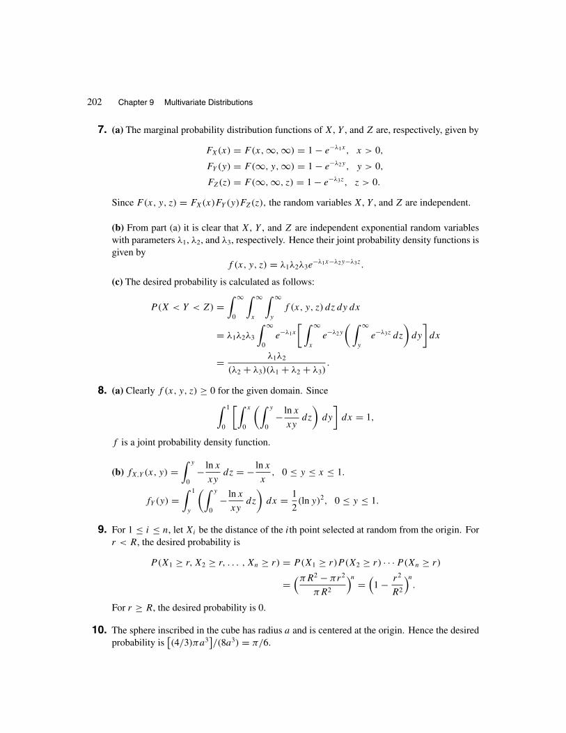
202 Chapter 9 Multivariate Distributions
7. (a) The marginal probability distribution functions of X, Y , and Z are, respectively, given by
FX(x) = F(x, ∞, ∞) = 1 − e−λ1x, x > 0,
FY (y) = F(∞, y, ∞) = 1 − e−λ2y, y > 0,
FZ(z) = F(∞, ∞, z) = 1 − e−λ3z, z > 0.
Since F(x, y, z) = FX(x)FY (y)FZ(z), the random variables X, Y , and Z are independent.
(b) From part (a) it is clear that X, Y , and Z are independent exponential random variableswith parameters λ1, λ2, and λ3, respectively. Hence their joint probability density functions isgiven by
f (x, y, z) = λ1λ2λ3e−λ1x−λ2y−λ3z.
(c) The desired probability is calculated as follows:
P(X < Y < Z) =∫ ∞
0
∫ ∞
x
∫ ∞
y
f (x, y, z) dz dy dx
= λ1λ2λ3
∫ ∞
0e−λ1x
[ ∫ ∞
x
e−λ2y
(∫ ∞
y
e−λ3z dz
)dy
]dx
= λ1λ2
(λ2 + λ3)(λ1 + λ2 + λ3).
8. (a) Clearly f (x, y, z) ≥ 0 for the given domain. Since∫ 1
0
[∫ x
0
(∫ y
0− ln x
xydz
)dy
]dx = 1,
f is a joint probability density function.
(b) fX,Y (x, y) =∫ y
0− ln x
xydz = − ln x
x, 0 ≤ y ≤ x ≤ 1.
fY (y) =∫ 1
y
(∫ y
0− ln x
xydz
)dx = 1
2(ln y)2, 0 ≤ y ≤ 1.
9. For 1 ≤ i ≤ n, let Xi be the distance of the ith point selected at random from the origin. Forr < R, the desired probability is
P(X1 ≥ r, X2 ≥ r, . . . , Xn ≥ r) = P(X1 ≥ r)P (X2 ≥ r) · · · P(Xn ≥ r)
=(πR2 − πr2
πR2
)n =(
1 − r2
R2
)n.
For r ≥ R, the desired probability is 0.
10. The sphere inscribed in the cube has radius a and is centered at the origin. Hence the desiredprobability is
[(4/3)πa3
]/(8a3) = π/6.

Section 9.1 Joint Distributions of n > 2 Random Variables 203
11. Yes, it is because f ≥ 0 and∫ ∞
0
∫ ∞
x1
∫ ∞
x2
· · ·∫ ∞
xn−1
e−xn dxn dxn−1 · · · dx1
=∫ ∞
0
∫ ∞
x1
∫ ∞
x2
· · ·∫ ∞
xn−2
e−xn−1 dxn−1 · · · dx1
= · · · =∫ ∞
0
∫ ∞
x1
e−x2 dx2 dx1 =∫ ∞
0e−x1 dx1 = 1.
12. Let f (x1, x2, x3) be the joint probability density function of X1, X2, and X3, the lifetimes ofthe original, the second, and the third transistors, respectively. We have that
f (x1, x2, x3) = 1
5e−x1/5 · 1
5e−x2/5 · 1
5e−x3/5 = 1
125e−(x1+x2+x3)/5.
Now
P(X1 + X2 + X3 < 15) =∫ 15
0
∫ 15−x1
0
∫ 15−x1−x2
0
1
125e−(x1+x2+x3)/5 dx3 dx2 dx1
=∫ 15
0
∫ 15−x1
0
[1
25e−(x1+x2)/5 − 1
25e−3
]dx2 dx1
=∫ 15
0
(1
5e−x1/5 − 4
5e−3 + 1
25e−3x1
)dx1
= 1 − 17
2e−3 = 0.5768.
Therefore, the desired probability is P(X1 + X2 + X3 ≥ 15) = 1 − 0.5768 = 0.4232.
13. Let F be the distribution function of X. We have that
F(t) = P(X ≤ t) = 1 − P(X > t) = 1 − P(X1 > t, X2 > t, . . . , Xn > t)
= 1 − P(X1 > t)P (X2 > t) · · · P(Xn > t) = 1 − e−λ1t e−λ2t · · · e−λnt
= 1 − e−(λ1+λ2+···+λn)t , t > 0.
Thus X is exponential with parameter λ1 + λ2 + · · · + λn.
14. Let Y be the number of functioning components of the system. The random variable Y isbinomial with parameters n and p. The reliability of this system is given by
r = P(X = 1) = P(Y ≥ k) =n∑
i=k
(n
i
)pi(1 − p)n−i .

204 Chapter 9 Multivariate Distributions
15. Let Xi be the lifetime of the ith part. The time until the item fails is the random variablemin(X1, X2, . . . , Xn) which by the solution to Exercise 13 is exponentially distributed withparameter nλ. Thus the average life of the item is 1/(nλ).
16. Let X1, X2, . . . be the lifetimes of the transistors selected at random. Clearly,
N = min{n : Xn > s
}.
Note that
P(XN ≤ t | N = n
) = P(Xn ≤ t | X1 ≤ s, X2 ≤ s, . . . , Xn−1 ≤ s, Xn > s).
This shows that for s ≥ t , P(XN ≤ t | N = n
) = 0. For s < t ,
P(XN ≤ t | N = n
) = P(s < Xn ≤ t, X1 ≤ s, X2 ≤ s, . . . , Xn−1 ≤ s)
P (X1 ≤ s, X2 ≤ s, . . . , Xn−1 ≤ s, Xn > s)
= P(s < Xn ≤ t)P (X1 ≤ s)P (X2 ≤ s) · · · P(Xn−1 ≤ s)
P (X1 ≤ s)P (X2 ≤ s) · · · P(Xn−1 ≤ s)P (Xn > s)
= P(s < Xn ≤ t)
P (Xn > s)= F(t) − F(s)
1 − F(s).
This relation shows that the probability distribution function of XN given N = n does notdepend on n. Therefore, XN and N are independent.
17. Clearly,
X = X1
[1 − (1 − X2)(1 − X3)
][1 − (1 − X4)(1 − X5X6)
]X7
= X1X7(X2X4 + X3X4 − X2X3X4 + X2X5X6 + X3X5X6
− X2X3X5X6 − X2X4X5X6 − X3X4X5X6 + X2X3X4X5X6).
The reliability of this system is
r = p1p7(p2p4 + p3p4 − p2p3p4 + p2p5p6 + p3p5p6
− p2p3p5p6 − p2p4p5p6 − p3p4p5p6 + p2p3p4p5p6).
18. Let G and F be the distribution functions of max1≤i≤n Xi and min1≤i≤n Xi , respectively. Letg and f be their probability density functions, respectively. For 0 ≤ t < 1,
G(t) = P(X1 ≤ t, X2 ≤ t, . . . , Xn ≤ t)
= P(X1 ≤ t)P (X2 ≤ t) · · · P(Xn ≤ t) = tn.

Section 9.1 Joint Distributions of n > 2 Random Variables 205
So
G(t) =
⎧⎪⎨⎪⎩0 t < 0
tn 0 ≤ t < 1
1 t ≥ 1.
Therefore,
g(t) = G′(t) ={
ntn−1 0 < t < 1
0 elsewhere.
This gives
E(
max1≤i≤n
Xi
) =∫ 1
0ntn dt = n
n + 1.
Similarly, for 0 ≤ t < 1,
F(t) = P(
min1≤i≤n
Xi ≤ t)
= 1 − P(
min1≤i≤n
Xi > t)
= 1 − P(X1 > t)P (X2 > t) · · · P(Xn > t)
= 1 − (1 − t)n, 0 ≤ t < 1.
Hence
F(t) =
⎧⎪⎨⎪⎩0 t < 0
1 − (1 − t)n 0 ≤ t < 1
1 t ≥ 1,
and
f (t) ={
n(1 − t)n−1 0 < t < 1
0 otherwise.
So
E(
min1≤i≤n
Xi
)=∫ 1
0nt (1 − t)n−1 dt = 1
n + 1.
19. We have that
P(
max(X1, X2, . . . , Xn) ≤ t) = P(X1 ≤ t, X2 ≤ t, . . . , Xn ≤ t)
= P(X1 ≤ t)P (X2 ≤ t) · · · P(Xn ≤ t)
= [F(t)
]n,
and
P(
min(X1, X2, . . . , Xn) ≤ t) = 1 − P
(min(X1, X2, . . . , Xn) > t
)= 1 − P(X1 > t, X2 > t, . . . , Xn > t)
= 1 − P(X1 > t)P (X2 > t) · · · P(Xn > t)
= 1 − [1 − F(t)
]n.

206 Chapter 9 Multivariate Distributions
20. We have that
P(Yn > x) = P(
min(X1, X2, . . . , Xn) >x
n
)= P
(X1 >
x
n, X2 >
x
n, . . . , Xn >
x
n
)= P
(X1 >
x
n
)P(X2 >
x
n
)· · · P
(Xn >
x
n
)=(
1 − x
n
)n
.
Thuslim
n→∞ P(Yn > x) = limn→∞
(1 − x
n
)n = e−x, x > 0.
21. We have that
P(X < Y < Z) =∫ ∞
−∞
∫ ∞
x
∫ ∞
y
h(x)h(y)h(z) dz dy dx
=∫ ∞
−∞
∫ ∞
x
h(x)h(y)[1 − H(y)
]dy dx
=∫ ∞
−∞h(x)
[−1
2
[1 − H(y)
]2]∞
x
dx
= 1
2
∫ ∞
−∞h(x)
[1 − H(x)
]2dx
= 1
2
[−1
3
[1 − H(x)
]3]∞
−∞= 1
6.
22. Noting that X2i = Xi , 1 ≤ i ≤ 5, we have
X = max{X2X5, X2X3X4, X1X4, X1X3X5}= 1 − (1 − X2X5)(1 − X2X3X4)(1 − X1X4)(1 − X1X3X5)
= X2X5 + X1X4 + X1X3X5 + X2X3X4 − X1X2X3X4 − X1X2X3X5
− X1X2X4X5 − X1X3X4X5 − X2X3X4X5 + 2X1X2X3X4X5.
Therefore, whenever the system is turned on for water to flow from A to B, water reaches Bwith probability r given by,
r = P(X = 1) = E(X) = p2p5 + p1p4 + p1p3p5 + p2p3p4 − p1p2p3p4
− p1p2p3p5 − p1p2p4p5 − p1p3p4p5 − p2p3p4p5 + 2p1p2p3p4p5.
23. Clearly, B = (1 × 1)/2 and h = 1. So the volume of the pyramid is (1/3)Bh = 1/6.
Therefore, the joint probability density function of X, Y , and Z is
f (x, y, z) ={
6 (x, y, z) ∈ V
0 otherwise.

Section 9.1 Joint Distributions of n > 2 Random Variables 207
Thus
fX(x) =∫ 1−x
0
(∫ 1−x−y
06 dz
)dy = 3(1 − x)2, 0 < x < 1.
Similarly, fY (y) = 3(1 − y)2, 0 < y < 1, and fZ(z) = 3(1 − z)2, 0 < z < 1. Since
f (x, y, z) �= fX(x)fY (y)fZ(z),
X, Y , and Z are not independent.
24. The probability that Ax2+Bx+C = 0 has real roots is equal to the probability that B2−4AC ≥0. To calculate this quantity, we will first evaluate the distribution functions of B2 and −4AC
and then use the convolution theorem to find the distribution function of B2 − 4AC.
FB2 (t) = P(B2 ≤ t) =
⎧⎪⎪⎨⎪⎪⎩0 if t < 0√
t if 0 ≤ t < 1
1 if t ≥ 1,
fB2 (t) = F ′
B2(t) =
⎧⎨⎩1
2√
tif 0 < t < 1
0 otherwise,
and
F−4AC(t) = P(−4AC ≤ t) =
⎧⎪⎪⎪⎨⎪⎪⎪⎩0 if t < −4
P(AC ≥ − t
4
)if −4 ≤ t < 0
1 if t ≥ 0.
Now A and C are random numbers from (0, 1); hence (A, C) is a random point from thesquare (0, 1) × (0, 1) in the ac-plane. Therefore, P(AC ≥ −t/4) = P
(C ≥ −t/(4A)
)is the
area of the shaded region(bounded by a = 1, c = 1, c = − t
4a
)of Figure 1.
c
a
-t/4
-t/4
1
10
Figure 1 The shaded region of Exercise 24.

208 Chapter 9 Multivariate Distributions
Thus, for −4 ≤ t < 0,
F−4AC(t) =∫ 1
−t/4
( ∫ 1
−t/(4a)
dc)da = 1 + t
4− t
4ln(− t
4
).
Therefore,
F−4AC(t) = P(−4AC ≤ t) =
⎧⎪⎪⎪⎨⎪⎪⎪⎩0 if t < −4
1 + t
4− t
4ln(− t
4
)if −4 ≤ t < 0
1 if t > 0.
Applying convolution theorem, we obtain
P(B2 − 4AC ≥ 0
) = 1 − P(B2 − 4AC < 0
)= 1 −
∫ ∞
−∞F−4AC
(0 − x)fB2 (x)dx
= 1 −∫ 1
0
(1 − x
4+ x
4ln
x
4
) 1
2√
xdx.
Letting y = √x/2, we get dy = 1
4√
xdx. So
P(B2 − 4AC ≥ 0
) = 1 −∫ 1/2
0(1 − y2 + y2 ln y2)2dy
= 1 −∫ 1/2
02dy + 2
∫ 1/2
0(y2 − y2 ln y2)dy
= 2∫ 1/2
0(y2 − y2 ln y2)dy.
Now by integration by parts (u = ln y2 , dv = y2dy),∫y2 ln y2dy = 1
3y3 ln y2 − 2
9y3.
Thus
P(B2 − 4AC ≥ 0
) =[10
9y3 − 2
3y3 ln y2
]1/2
0= 5
36+ 1
6ln 2 ≈ 0.25.
25. The following solution by Scott Harrington, Duke University, Durham, NC, was given in TheCollege Mathematics Journal, September 1993.
Let V be the set of points (A, B, C) ∈ [0, 1]3 such that f (x) = x3+Ax2+Bx+C = 0has all real roots. The probability that all of the roots are real is the volume of V .

Section 9.1 Joint Distributions of n > 2 Random Variables 209
The function is cubic, so it either has one real root and two complex roots orthree real roots. Since the coefficient of x3 is positive, limx→−∞ f (x) = −∞ andlimx→+∞ f (x) = +∞. The number of real roots of the graph of f (x) depends onthe nature of the critical points of the function f .
f ′(x) = 3x2 + 2Ax + B = 0,
with roots
x = −1
3A ± 1
3
√A2 − 3B.
Let D = √A2 − 3B, x1 = −1
3(A + D), and x2 = −1
3(A − D). If A2 < 3B then the
critical points are imaginary, so the graph of f (x) is strictly increasing and theremust be exactly one real root. Thus we may assume A2 ≥ 3B.
In order for there to be three real roots, counting multiplicities, the local maximum(x1, f (x1)
)and local minimum
(x2, f (x2)
)must satisfy f (x1) ≥ 0 and f (x2) ≤ 0;
that is,
f (x1) = − 1
27(A3 + 3A2D + 3AD2 + D3)
+ 1
9A(A2 + 2AD + D2) − 1
3B(A + D) + C ≥ 0,
f (x2) = − 1
27(A3 − 3A2D + 3AD2 − D3)
+ 1
9A(A2 − 2AD + D2) − 1
3B(A − D) + C ≤ 0.
Simplifying produces two half-spaces:
C ≥ 1
27
(− 2A3 + 9AB − 2(A2 − 3B)3/2
), (constraint surface 1);
C ≤ 1
27
(− 2A3 + 9AB + 2(A2 − 3B)3/2
), (constraint surface 2).
These two surfaces intersect at the curve given parametrically by A = t , B = 1
3t2
and C = 1
27t3. Note that all points in the intersection of these two half-spaces
satisfy B ≤ 1
3A2. Surface 2 intersects the plane C = 0 at the A-axis, but surface 1
intersects the plane C = 0 at the curve B = 1
4A2, which is a quadratic curve in the
plane C = 0 located between the A-axis and the upper limit B = 13A2. Therefore, V
is the region above the plane C = 0 and constraint surface 1, and below constraintsurface 2. The volume of V is the volume V2 under surface 2 minus the volume V1under surface 1. Now
V1 =∫ 1
a=0
∫ (1/3)a2
b=(1/4)a2
1
27
(− 2a3 + 9ab − 2(a2 − 3b)3/2
)db da

210 Chapter 9 Multivariate Distributions
=∫ 1
0
1
27
[− 2a3b + 9
2ab2 + 4
15(a2 − 3b)5/2
](1/3)a2
b=(1/4)a2
da
=∫ 1
0
1
27· 7
160a5 da = 7
25, 920, and
V2 =∫ 1
a=0
∫ (1/3)a2
b=0
1
27
(− 2a3 + 9ab + 2(a2 − 3b)3/2
)db da
=∫ 1
0
1
27
[− 2a3b + 9
2ab2 − 4
15(a2 − 3b)5/2
](1/3)a2
b=0
da =∫ 1
0
1
270a5 da = 1
1620.
Thus
V = V2 − V1 = 1
1, 620− 7
25, 920= 1
2, 880.
9.2 ORDER STATISTICS
1. By Theorem 9.5, we have that
f3(x) = 4!2! 1!f (x)
[F(x)
]2[1 − F(x)
],
where
f (x) =⎧⎨⎩1 0 < x < 1
0 otherwise,
and
F(x) =
⎧⎪⎪⎪⎨⎪⎪⎪⎩0 x < 0
x 0 ≤ x < 1
1 x ≥ 1.
Therefore,f3(x) = 12x2(1 − x), 0 < x < 1.
Hence the desired probability is∫ 1/2
1/412x2(1 − x) dx = 67
256= 0.26172.
2. Let X1 and X2 be the points selected at random. By Theorem 9.6, the joint probability densityfunction of X(1) and X(2) is given by
f12(x, y) = 2!(1 − 1)! (2 − 1 − 1)! (2 − 2)! x1−1(y − x)2−1−1, 0 < x < y < 1.

Section 9.2 Order Statistics 211
Sof12(x, y) = 2, 0 < x < y < 1.
We have that, the desired probability is given by
P(X(2) ≥ 3X(1)
) =∫ 1
0
∫ y/3
02 dx dy = 1
3.
3. By Theorem 9.5, f4(x), the probability density function of X(4) is given by
f4(x) = 4!3! 0!λe−λx
(1 − e−λx
)3(e−λx
)4−4 = 4λe−λx(1 − e−λx
)3.
The desired probability is∫ ∞
3λ
4λe−λx(1 − e−λx
)3dx = 1 − (
1 − e−3λ2)4.
4. By Remark 6.4,
E[X(n)
] =∫ ∞
0P(X(n) > x) dx.
Now
P(X(n) > x
) = 1 − P(X(n) ≤ x
)= 1 − P(X1 ≤ x, X2 ≤ x, . . . , Xn ≤ x) = 1 − [
F(x)]n
.
So
E[X(n)
] =∫ ∞
0
(1 − [
F(x)]n)
dx.
5. To find P(X(i) = k
), 0 ≤ k ≤ n, note that
P(X(i) = k
) = 1 − P(X(i) < k
)− P(X(i) > k
).
Let N be the number of Xj ’s that are less than k. Then N is a binomial random variable withparameters m and
p1 =k−1∑l=0
(n
l
)pl(1 − p)n−l . (35)
Let L be the number of Xj ’s that are greater than k. Then L is a binomial random variablewith parameters m and
p2 =n∑
l=k+1
(n
l
)pl(1 − p)n−l . (36)

212 Chapter 9 Multivariate Distributions
Clearly,
P(X(i) < k
) = P(N ≥ i) =m∑
j=i
(m
j
)p
j
1(1 − p1)m−j ,
and
P(X(i) > k
) = P(L ≥ m − i + 1) =m∑
j=m−i+1
(m
j
)p
j
2(1 − p2)m−j .
Thus, for 0 ≤ k ≤ n,
P(X(i) = k
) = 1 −m∑
j=i
(m
j
)p
j
1(1 − p1)m−j −
m∑j=m−i+1
(m
j
)p
j
2(1 − p2)m−j ,
where p1 and p2 are given by (35) and (36).
6. By Theorem 9.6, the joint probability density function of X(1) and X(n) is given by
f1n(x, y) = n(n − 1)f (x)f (y)[F(y) − F(x)
]n−2, x < y.
Therefore,
G(t) = P
(X(1) + X(n)
2≤ t
)= P
(X(1) + X(n) ≤ 2t
)=∫ t
−∞
∫ 2t−x
x
n(n − 1)f (x)f (y)[F(y) − F(x)
]n−2dy dx
= n
∫ t
−∞
[F(2t − x) − F(x)
]n−1f (x) dx.
7. By Theorem 9.5, f1(x), the probability density function of X(1) is given by
f1(x) = 2!(1 − 1)! (2 − 1)!λe−λx
(1 − e−λx
)1−1(e−λx
)2−1 = 2λe−2λx, x ≥ 0.
By Theorem 9.6, f12(x, y), the joint probability density function of X(1) and X(2) is given by
f12(x, y) = 2!(1 − 1)! (2 − 1 − 1)! (2 − 2)! λe−λxλe−λy
= (1 − e−λx
)1−1(e−λx − e−λy
)2−1−1 = 2λ2e−λ(x+y), 0 ≤ x < y < ∞.
Let U = X(1) and V = X(2) − X(1). We will show that g(u, v), the joint probability densityfunction of U and V satisfy g(u, v) = gU(u)gV (v). This proves that U and V are independent.To find g(u, v), note that the system of two equations in two unknowns{
x = u
y − x = v
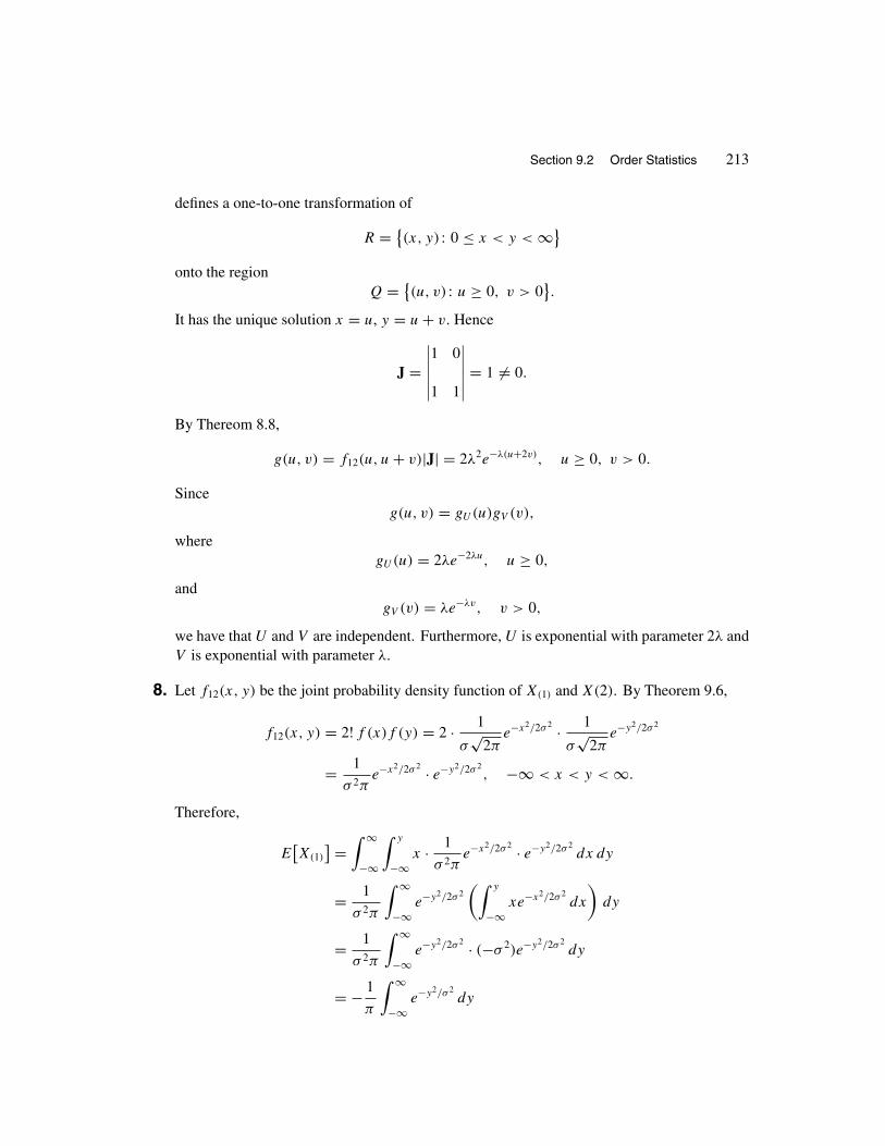
Section 9.2 Order Statistics 213
defines a one-to-one transformation of
R = {(x, y) : 0 ≤ x < y < ∞}
onto the regionQ = {
(u, v) : u ≥ 0, v > 0}.
It has the unique solution x = u, y = u + v. Hence
J =∣∣∣∣∣∣1 0
1 1
∣∣∣∣∣∣ = 1 �= 0.
By Thereom 8.8,
g(u, v) = f12(u, u + v)|J| = 2λ2e−λ(u+2v), u ≥ 0, v > 0.
Sinceg(u, v) = gU(u)gV (v),
wheregU(u) = 2λe−2λu, u ≥ 0,
andgV (v) = λe−λv, v > 0,
we have that U and V are independent. Furthermore, U is exponential with parameter 2λ andV is exponential with parameter λ.
8. Let f12(x, y) be the joint probability density function of X(1) and X(2). By Theorem 9.6,
f12(x, y) = 2! f (x)f (y) = 2 · 1
σ√
2πe−x2/2σ 2 · 1
σ√
2πe−y2/2σ 2
= 1
σ 2πe−x2/2σ 2 · e−y2/2σ 2
, −∞ < x < y < ∞.
Therefore,
E[X(1)
] =∫ ∞
−∞
∫ y
−∞x · 1
σ 2πe−x2/2σ 2 · e−y2/2σ 2
dx dy
= 1
σ 2π
∫ ∞
−∞e−y2/2σ 2
(∫ y
−∞xe−x2/2σ 2
dx
)dy
= 1
σ 2π
∫ ∞
−∞e−y2/2σ 2 · (−σ 2)e−y2/2σ 2
dy
= − 1
π
∫ ∞
−∞e−y2/σ 2
dy
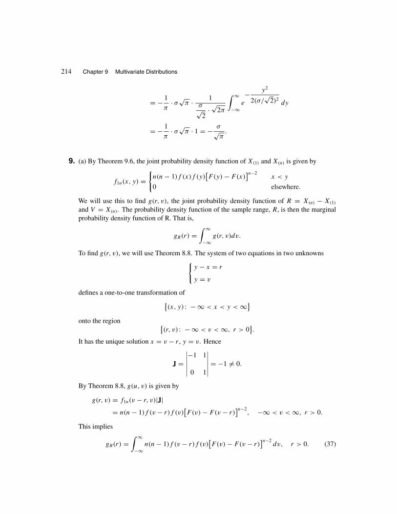
214 Chapter 9 Multivariate Distributions
= − 1
π· σ
√π · 1
σ√2
· √2π
∫ ∞
−∞e
− y2
2(σ/√
2)2dy
= − 1
π· σ
√π · 1 = − σ√
π.
9. (a) By Theorem 9.6, the joint probability density function of X(1) and X(n) is given by
f1n(x, y) ={
n(n − 1)f (x)f (y)[F(y) − F(x)
]n−2x < y
0 elsewhere.
We will use this to find g(r, v), the joint probability density function of R = X(n) − X(1)
and V = X(n). The probability density function of the sample range, R, is then the marginalprobability density function of R. That is,
gR(r) =∫ ∞
−∞g(r, v)dv.
To find g(r, v), we will use Theorem 8.8. The system of two equations in two unknowns{y − x = r
y = v
defines a one-to-one transformation of{(x, y) : − ∞ < x < y < ∞}
onto the region {(r, v) : − ∞ < v < ∞, r > 0
}.
It has the unique solution x = v − r , y = v. Hence
J =∣∣∣∣∣∣−1 1
0 1
∣∣∣∣∣∣ = −1 �= 0.
By Theorem 8.8, g(u, v) is given by
g(r, v) = f1n(v − r, v)|J|= n(n − 1)f (v − r)f (v)
[F(v) − F(v − r)
]n−2, −∞ < v < ∞, r > 0.
This implies
gR(r) =∫ ∞
−∞n(n − 1)f (v − r)f (v)
[F(v) − F(v − r)
]n−2dv, r > 0. (37)

Section 9.3 Multinomial Distributions 215
(b) The probability density function of n random numbers from (0, 1) is obtained by letting
f (v) =⎧⎨⎩1 0 < v < 1
0 otherwise,
and F(v) − F(v − r) = v − (v − r) = r in (37). Note that the integrand of the integral in(37) is nonzero if 0 < v < 1 and if 0 < v − r < 1; that is, if 0 < r < v < 1. Therefore,
gR(r) =∫ 1
r
n(n − 1)rn−2 dv = n(n − 1)rn−2(1 − r), 0 < r < 1.
10. Let f and F be the probability density and distribution functions of Xi , 1 ≤ i ≤ n, respectively.We have that
f (x) =⎧⎨⎩1/θ 0 < x < θ
0 elsewhere
and
F(x) =
⎧⎪⎪⎪⎨⎪⎪⎪⎩0 x < 0
x/θ 0 ≤ x < θ
1 x ≥ θ.
Let g(r) be the probability density function of R = X(n) − X(1). By part (a) of Exercise 9,
g(r) =∫ θ
r
n(n − 1)(v
θ− v − r
θ
)n−2dv = n(n − 1)rn−2
θn(θ − r) 0 < r < θ.
(Note that 0 < v < θ and 0 < v − r < θ imply that r < v < θ .) Therefore,
E(R) =∫ ∞
0rn(n − 1)rn−2
θn(θ − r) dr = n − 1
n + 1θ.
9.3 MULTINOMIAL DISTRIBUTIONS
1. The desired probability is
8!3! 2! 3!
(150
800
)3 (400
800
)2 (250
800
)3
= 0.028.
2. We have that
P(B = i, R = j, G = 20 − i − j)
= 20!i! j ! (20 − i − j)!(0.2)i(0.3)j (0.5)20−i , 0 ≤ i, j ≤ 20, i + j ≤ 20.

216 Chapter 9 Multivariate Distributions
3. Let U , D, and S be the number of days among the next six days that the stock market movesup, moves down, and remains the same, respectively. The desired probability is
P(U = 0, D = 0, S = 6) + P(U = 1, D = 1, S = 4)
+ P(U = 2, D = 2, S = 2) + P(U = 3, D = 3, S = 0)
= 6!0! 0! 6!
(1
4
)0 ( 5
12
)0 (1
3
)6
+ 6!1! 1! 4!
(1
4
)1 ( 5
12
)1 (1
3
)4
+ 6!2! 2! 2!
(1
4
)2 ( 5
12
)2 (1
3
)2
+ 6!3! 3! 0!
(1
4
)3 ( 5
12
)3 (1
3
)0
= 0.171.
4. Let A, B, C, D, and F be the number of students who get A, B, C, D, and F, respectively. Thedesired probability is given by
P(A = 2, B = 5, C = 5, D = 2, F = 1) + P(A = 3, B = 5, C = 5, D = 2, F = 0)
= 15!2! 5! 5! 2! 1!(0.16)2(0.34)5(0.34)5(0.14)2(0.02)1
+ 15!3! 5! 5! 2! 0!(0.16)3(0.34)5(0.34)5(0.14)2(0.02)0
= 0.0172.
5. Let L, M , and S be the number of large, medium, and small watermelons among the fivewatermelons Joanna buys, respectively.(a) We have that
P(L ≥ 2) = 1 − P(L = 0) − P(L = 1)
= 1 −(
5
0
)(0.50)0(0.50)5 −
(5
1
)(0.50)1(0.50)4 = 0.8125.
(b) P(L = 2, M = 2, S = 1) = 5!2! 2! 1!(0.5)2(0.3)2(0.2)1 = 0.135.
(c) Using parts (a) and (b) and
P(L = 3, M = 2, S = 0) = 5!3! 2! 0!(0.5)3(0.3)2(0.2)0 = 0.1125,
we have that
P(M = 2 | L ≥ 2) = P(M = 2, L ≥ 2)
P (L ≥ 2)
= P(L = 2, M = 2, S = 1) + P(L = 3, M = 2, S = 0)
P (L ≥ 2)
= 0.135 + 0.1125
0.8125= 0.3046.

Section 9.3 Multinomial Distributions 217
6. Let X be the number of faculty members who are below 40 and Y be the number of those whoare above 50 in the committee. The desired probability mass function is
pX|Y (x|2) =10!
x! 2! (8 − x)!(0.5)x(0.3)2(0.2)8−x
(10
2
)(0.3)2(0.7)8
=(
8
x
)(5
7
)x (2
7
)8−x
, 0 ≤ x ≤ 8.
7. The probability is 1/4 that the blood type of a child of this man and woman is AB. Theprobability is 1/4 that it is A, and the probability is 1/2 that it is B. The desired probability isequal to
6!3! 2! 1!
(1
2
)3(1
4
)2(1
4
)1 = 15
128= 0.117.
8. The probability of two AA’s, two Aa’s, and two aa’s is
g(p) = 6!2! 2! 2!(p
2)2[2p(1 − p)
]2[(1 − p)2
]2 = 360p6(1 − p)6.
To find the maximum of this function, set g′(p) = 0 to obtain p = 1/2.
9. Let N(t) be the number of customers who arrive at the store by time t . We are given that{N(t) : t ≥ 0
}is a Poisson process with λ = 3. Let X, Y , and Z be the number of cus-
tomers who use charge cards, write personal checks, and pay cash in five operating minutes,respectively. Then
P(X = 5, Y = 2, Z = 3)
=∞∑
n=10
P(X = 5, Y = 2, Z = 3 | N(5) = n
)P(N(5) = n
)
=∞∑
n=10
n!5! 2! 3! (n − 10)!(0.40)5(0.10)2(0.20)3(0.30)n−10 · e−1515n
n!
= (0.40)5(0.10)2(0.20)3e−151510
3! 5! 2!∞∑
n=10
(0.30)n−10(15)n−10
(n − 10)!
= (0.00010035)
∞∑n=10
(4.5)n−10
(n − 10)! = (0.00010035)e4.5 = 0.009033.
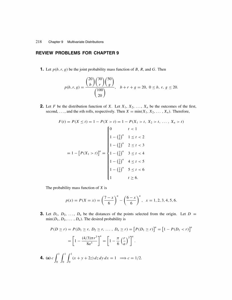
218 Chapter 9 Multivariate Distributions
REVIEW PROBLEMS FOR CHAPTER 9
1. Let p(b, r, g) be the joint probability mass function of B, R, and G. Then
p(b, r, g) =
(20
b
)(30
r
)(50
g
)(
100
20
) , b + r + g = 20, 0 ≤ b, r, g ≤ 20.
2. Let F be the distribution function of X. Let X1, X2, . . . , Xn be the outcomes of the first,second, . . . , and the nth rolls, respectively. Then X = min(X1, X2, . . . , Xn). Therefore,
F(t) = P(X ≤ t) = 1 − P(X > t) = 1 − P(X1 > t, X2 > t, . . . , Xn > t)
= 1 − [P(X1 > t)
]n =
⎧⎪⎪⎪⎪⎪⎪⎪⎪⎪⎪⎪⎪⎪⎪⎪⎪⎨⎪⎪⎪⎪⎪⎪⎪⎪⎪⎪⎪⎪⎪⎪⎪⎪⎩
0 t < 1
1 − (56
)n1 ≤ t < 2
1 − (46
)n2 ≤ t < 3
1 − (36
)n3 ≤ t < 4
1 − (26
)n4 ≤ t < 5
1 − (16
)n5 ≤ t < 6
1 t ≥ 6.
The probability mass function of X is
p(x) = P(X = x) =(
7 − x
6
)n
−(
6 − x
6
)n
, x = 1, 2, 3, 4, 5, 6.
3. Let D1, D2, . . . , Dn be the distances of the points selected from the origin. Let D =min(D1, D2, . . . , Dn). The desired probability is
P(D ≥ r) = P(D1 ≥ r, D2 ≥ r, . . . , Dn ≥ r) = [P(D1 ≥ r)
]n = [1 − P(D1 < r)
]n=[
1 − (4/3)πr3
8a3
]n
=[
1 − π
6
( r
a
)3]n
.
4. (a) c
∫ 1
0
∫ 1
0
∫ 1
0(x + y + 2z) dz dy dx = 1 �⇒ c = 1/2.

Chapter 9 Review Problems 219
(b) We have that
P(X <
1
3
∣∣∣ Y <1
2, Z <
1
4
)=
P(X <
1
3, Y <
1
2, Z <
1
4
)P(Y <
1
2, Z <
1
4
)
=
∫ 1/3
0
∫ 1/2
0
∫ 1/4
0
1
2(x + y + 2z) dz dy dx∫ 1
0
∫ 1/2
0
∫ 1/4
0
1
2(x + y + 2z) dz dy dx
= 1/36
1/8= 2
9.
5. The joint probability mass function of the number of times each face appears is multinomial.
Hence the desired probability is18!(3!)6
(1
6
)18
= 0.00135.
6. Using the multinomial distribution, the answer is
7!3! 2! 2!(0.4)3(0.35)2(0.25)2 = 0.1029.
7. For 1 ≤ i ≤ n, let Xi be the lifetime of the ith component. Thenmin(X1, X2, . . . , Xn) is the lifetime of the system. Let F (t) be the survival function ofthe system. By the independence of the lifetimes of the components, for all t > 0,
F (t) = P(
min(X1, X2, . . . , Xn) > t) = P(X1 > t, X2 > t, . . . , Xn > t)
= P(X1 > t)P (X2 > t) · · · P(Xn > t) = F1(t)F2(t) · · · Fn(t).
8. For 1 ≤ i ≤ n, let Xi be the lifetime of the ith component. Thenmax(X1, X2, . . . , Xn) is the lifetime of the system. Let F (t) be the survival function ofthe system. By the independence of the lifetimes of the components, for all t > 0,
F (t) = P(
max(X1, X2, . . . , Xn) > t)
= 1 − P(
max(X1, X2, . . . , Xn) ≤ t)
= 1 − P(X1 ≤ t, X2 ≤ t, . . . , Xn ≤ t)
= 1 − P(X1 ≤ t)P (X2 ≤ t) · · · P(Xn ≤ t)
= 1 − F1(t)F2(t) · · · Fn(t).
9. The problem is equivalent to the following: Two points X and Y are selected independentlyand at random from the interval (0, �). What is the probability that the length of at least one

220 Chapter 9 Multivariate Distributions
interval is less than �/20? The solution to this problem is as follows:
P(
min(X, Y − X, � − Y ) <�
20
∣∣∣ X < Y)P(X < Y)
+ P(
min(Y, X − Y, � − X) <�
20
∣∣∣ X > Y)P(X > Y)
= 2P(
min(X, Y − X, � − Y ) <�
20
∣∣∣ X < Y)P(X < Y)
= 2P(
min(X, Y − X, � − Y ) <�
20
∣∣∣ X < Y)
· 1
2
= 1 − P(
min(X, Y − X, � − Y ) ≥ �
20
∣∣∣ X < Y)
= 1 − P(X ≥ �
20, Y − X ≥ �
20, � − Y ≥ �
20
∣∣∣ X < Y)
= 1 − P(X ≥ �
20, Y − X ≥ �
20, Y ≤ 19�
20
∣∣∣ X < Y).
Now P(X ≥ �
20, Y − X ≥ �
20, Y ≤ 19�
20
∣∣∣ X < Y)
is the area of the region{(x, y) ∈ R2 : 0 < x < �, 0 < y < �, x ≥ �
20, y − x ≥ �
20, y ≤ 19�
20
}divided by the area of the triangle{
(x, y) ∈ R2 : 0 < x < �, 0 < y < �, y > x};
that is,17�
20× 17�
202
÷ �2
2= 0.7225.
Therefore, the desired probability is 1 − 0.7225 = 0.2775.
10. Let f13(x, y) be the joint probability density function of X(1) and X(3). By Theorem 9.6,
f13(x, y) = 6(y − x), 0 < x < y < 1.
Let U = X(1) + X(3)
2and V = X(1). Using Theorem 8.8, we will find g(u, v), the joint
probability density function of U and V . The probability density function of the midrange ofthese three random variables is gU(u). The system of two equations in two unknowns⎧⎨⎩
x + y
2= u
x = v

Chapter 9 Review Problems 221
defines a one-to-one transformation of
R = {(x, y) : 0 < x < y < 1
}onto the region
Q ={(u, v) : 0 < v < u <
v + 1
2< 1
}that has the unique solution {
x = v
y = 2u − v.
Hence
J =∣∣∣∣∣∣0 1
2 −1
∣∣∣∣∣∣ = −2 �= 0;
therefore,
g(u, v) = f13(v, 2u − v)|J| = 24(u − v), 0 < v < u <v + 1
2< 1.
To find gU(u), draw the region Q to see that
gU(u) =
⎧⎪⎪⎪⎪⎨⎪⎪⎪⎪⎩
∫ u
024(u − v) dv 0 < u < 1/2
∫ u
2u−124(u − v) dv 1/2 ≤ u < 1.
Therefore,
gU(u) =
⎧⎪⎨⎪⎩12u2 0 < u < 1/2
12(u − 1)2 1/2 ≤ u < 1.
The expected value of U is given by
E(U) =∫ 1/2
012u3 du +
∫ 1
1/212u(u − 1)2 du = 3
16+ 5
16= 1
2.

Chapter 10
More Expectations
and Variances
10.1 EXPECTED VALUES OF SUMS OF RANDOM VARIABLES
1. Since
E(X) =∫ 1
0x(1 − x) dx +
∫ 2
1x(x − 1) dx = 2
3,
and
E(X2) =∫ 1
0x2(1 − x) dx +
∫ 2
1x2(x − 1) dx = 3
2,
we have that
E(X2 + X) = 3
2+ 2
3= 13
6.
2. By Example 10.7, the answer is5
2/5= 12.5.
3. We have that E(X2) = Var(X) + [E(X)
]2 = 1. Similarly, E(Y 2) = E(Z2) = 1. Thus
E[X2(Y + 5Z)2
] = E(X2)E[(Y + 5Z)2
] = E(Y 2 + 25Z2 + 10YZ)
= E(Y 2) + 25E(Z2) + 10E(Y )E(Z) = 26.
4. Since f (x, y) = e−x · 2e−2y , X and Y are independent exponential random variables withparameters 1 and 2, respectively. Thus E(X) = 1, E(Y ) = 1/2,
E(X2) = Var(X) + [E(X)
]2 = 1 + 1 = 2,
and
E(Y 2) = Var(Y ) + [E(Y )
]2 = 1
4+ 1
4= 1
2.
Therefore, E(X2 + Y 2) = 2 + 1
2= 5
2.

Section 10.1 Expected Values of Sums of Random Variables 223
5. let X1, X2, X3, X4, and X5 be geometric random variables with parameters 1, 4/5, 3/5, 2/5,and 1/5, respectively. The desired quantity is
E(X1 + X2 + X3 + X4 + X5) = E(X1) + E(X2) + E(X3) + E(X4) + E(X5)
= 1 + 5
4+ 5
3+ 5
2+ 5 = 11.42.
6. Clearly,
E(Xi) = 1 · 1
n+ 0 ·
(1 − 1
n
)= 1
n.
Thus E(X1 + X2 + · · · + Xn) = n · 1
n= 1 is the desired quantity.
7. Let X1, X2, X3, and X4 be the cost of a band to play music, the amount the caterer will charge,the rent of a hall to give the party, and other expenses, respectively. Let N be the numberof people who participate. We have that E(X1) = 1550, E(X2) = 1900, E(X3) = 1000,E(X4) = 550, and
E(N) =200∑
i=151
i · 1
50= 1
50
( 200∑i=1
i −150∑i=1
i)
= 1
50
(200 × 201
2− 150 × 151
2
)= 175.50.
To have no loss on average, let x be the amount (in dollars) that the society should charge eachparticipant. We must have
E(X1 + X2 + X3 + X4) ≤ E(xN) = xE(N).
This gives
x ≥ E(X1) + E(X2) + E(X3) + E(X4)
175.50= 1550 + 1900 + 1000 + 550
175.50= 28.49.
So to have no loss on the average, the society should charge each participant $28.49.
8. (a) E(→ 007) = E(007 → 007) = 1, 000.
(b)
E(→ 156156) = E(→ 156) + E(156 → 156156)
= E(156 → 156) + E(156156 → 156156)
= 1, 000 + 1, 000, 000 = 1, 001, 000.
(c)
E(→ 575757) = E(→ 57) + E(57 → 5757) + E(5757 → 575757)
= E(57 → 57) + E(5757 → 5757) + E(575757 → 575757)
= 100 + 10, 000 + 1, 000, 000 = 1, 010, 100.

224 Chapter 10 More Expectations and Variances
9. Let X be the number of students standing at the front of the room after k, 1 ≤ k < n nameshave been called. The k students whose names have been called are not standing. Let A1, A2,. . . , An−k be the students whose names have not been called. Let
Xi ={
1 if Ai is standing
0 otherwise.
Clearly,X = X1 + X2 + · · · + Xn−k.
For i, 1 ≤ i ≤ n − k,
E(Xi) = P(Ai is standing
) = k
n.
This is because Ai is standing if and only if his or her original seat was among the first k.Hence
E(X) = E(X1) + E(X2) + · · · + E(Xn−k) = (n − k) · k
n= (n − k)k
n.
10. By Theorem 10.2,
E[min(X1, X2, . . . , Xn)
] =∞∑
k=1
P(min(X1, X2, . . . , Xn) ≥ k
)=
∞∑k=1
P(X1 ≥ k, X2 ≥ k, . . . Xn ≥ k)
=∞∑
k=1
P(X1 ≥ k)P (X2 ≥ k) · · · P(Xn ≥ k)
=∞∑
k=1
[P(X1 ≥ k)
]n =∞∑
k=1
[( ∞∑i=k
pi
)n]
=∞∑
k=1
hnk .
11. Let E1 be the event that the first three outcomes are heads and the fourth outcome is tails.For 2 ≤ i ≤ n − 3, let Ei be as defined in the hint. Let En−2 be the event that the outcome(n − 3) is tails and the last three outcomes are heads. The expected number of exactly threeconsecutive heads is
E(X1 +
n−3∑i=2
Xi + Xn−2
)= E(X1) +
n−3∑i=2
E(Xi) + E(Xn−2)
= P(E1) +n−3∑i=2
P(Ei) + P(En−2)
=(1
2
)4 +n−3∑i=2
(1
2
)5 +(1
2
)4
=(1
2
)3 + (n − 4)(1
2
)5 = n
32.
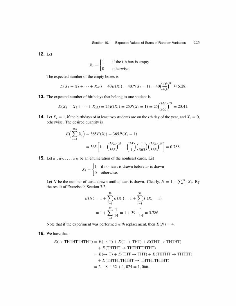
Section 10.1 Expected Values of Sums of Random Variables 225
12. Let
Xi ={
1 if the ith box is empty
0 otherwise;
The expected number of the empty boxes is
E(X1 + X2 + · · · + X40) = 40E(Xi) = 40P(Xi = 1) = 40(39
40
)80 ≈ 5.28.
13. The expected number of birthdays that belong to one student is
E(X1 + X2 + · · · + X25) = 25E(Xi) = 25P(Xi = 1) = 25(364
365
)24 = 23.41.
14. Let Xi = 1, if the birthdays of at least two students are on the ith day of the year, and Xi = 0,otherwise. The desired quantity is
E( 365∑
i=1
Xi
)= 365E(Xi) = 365P(Xi = 1)
= 365
[1 −
(364
365
)25 −(
25
1
)( 1
365
)(364
365
)24]
= 0.788.
15. Let u1, u2, . . . , u39 be an enumeration of the nonheart cards. Let
Xi ={
1 if no heart is drawn before ui is drawn
0 otherwise.
Let N be the number of cards drawn until a heart is drawn. Clearly, N = 1 +∑39i=1 Xi . By
the result of Exercise 9, Section 3.2,
E(N) = 1 +39∑i=1
E(Xi) = 1 +39∑i=1
P(Xi = 1)
= 1 +39∑i=1
1
14= 1 + 39 · 1
14= 3.786.
Note that if the experiment was performed with replacement, then E(N) = 4.
16. We have that
E(→ THTHTTHTHT) = E(→ T) + E(T → THT) + E(THT → THTHT)
+ E(THTHT → THTHTTHTHT)
= E(→ T) + E(THT → THT) + E(THTHT → THTHT)
+ E(THTHTTHTHT → THTHTTHTHT)
= 2 + 8 + 32 + 1, 024 = 1, 066.

226 Chapter 10 More Expectations and Variances
17. (a)∫ ∞
0
∫ ∞
0I (x, y) dx dy is the area of the rectangle
{(x, y) ∈ R2 : 0 ≤ x < X, 0 ≤ y < Y
};therefore it is equal to XY .
(b) Part (a) implies that
E(XY) =∫ ∞
0
∫ ∞
0E[I (x, y)
]dx dy =
∫ ∞
0
∫ ∞
0P(X > x, Y > y) dx dy.
18. Clearly N > i if and only if
X1 ≥ X2 ≥ X3 ≥ · · · ≥ Xi.
Hence for i ≥ 2,
P(N > i) = P(X1 ≥ X2 ≥ X3 ≥ · · · ≥ Xi−1 ≥ Xi
) = 1
i!because Xi’s are independent and identically distributed. So, by Theorem 10.2,
E(N) =∞∑i=1
P(N ≥ i) =∞∑i=0
P(N > i) = P(N > 0) + P(N > 1) +∞∑i=2
1
i!
= 1 + 1 +∞∑i=2
1
i! =∞∑i=0
1
i! = e.
19. If the first red chip is drawn on or before the 10th draw, let N be the number of chips beforethe first red chip. Otherwise, let N = 10. Clearly,
P(N = i) =(1
2
)i(1
2
)=(1
2
)i+1, 0 ≤ i ≤ 9; P(N = 10) =
(1
2
)10.
The desired quantity is
E(10 − N) =9∑
i=0
(10 − i)(1
2
)i+1 + (10 − 10) ·(1
2
)10 ≈ 9.001.
20. Clearly, if for some λ ∈ R, X = λY , Cauchy-Schwarz’s inequality becomes equality. Weshow that the converse of this is also true. Suppose that for random variables X and Y ,
E(XY) =√
E(X2)E(Y 2).
Then4[E(XY)
]2 − 4E(X2)E(Y 2) = 0.
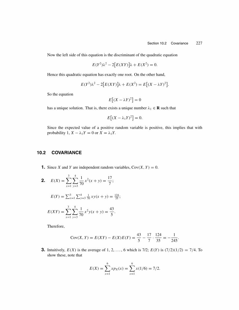
Section 10.2 Covariance 227
Now the left side of this equation is the discriminant of the quadratic equation
E(Y 2)λ2 − 2[E(XY)
]λ + E(X2) = 0.
Hence this quadratic equation has exactly one root. On the other hand,
E(Y 2)λ2 − 2[E(XY)
]λ + E(X2) = E
[(X − λY )2
].
So the equationE[(X − λY )2
] = 0
has a unique solution. That is, there exists a unique number λ1 ∈ R such that
E[(X − λ1Y )2
] = 0.
Since the expected value of a positive random variable is positive, this implies that withprobability 1, X − λ1Y = 0 or X = λ1Y.
10.2 COVARIANCE
1. Since X and Y are independent random variables, Cov(X, Y ) = 0.
2. E(X) =3∑
x=1
4∑y=3
1
70x2(x + y) = 17
7;
E(Y ) = ∑3x=1
∑4y=3
170 xy(x + y) = 124
35 ;
E(XY) =3∑
x=1
4∑y=3
1
70x2y(x + y) = 43
5.
Therefore,
Cov(X, Y ) = E(XY) − E(X)E(Y ) = 43
5− 17
7· 124
35= − 1
245.
3. Intuitively, E(X) is the average of 1, 2, . . . , 6 which is 7/2; E(Y ) is (7/2)(1/2) = 7/4. Toshow these, note that
E(X) =6∑
x=1
xpX(x) =6∑
x=1
x(1/6) = 7/2.

228 Chapter 10 More Expectations and Variances
By the table constructed for p(x, y) in Example 8.2,
E(Y ) = 0 · 63
384+ 1 · 120
384+ 2 · 99
384+ 3 · 64
384+ 4 · 29
384+ 5 · 8
384+ 6 · 1
384= 7
4.
By the same table,
E(XY) =6∑
x=1
6∑y=0
xyp(x, y) = 91/12.
Therefore,
Cov(X, Y ) = E(XY) − E(X)E(Y ) = 91
12− 7
2· 7
4= 35
24> 0.
This shows that X and Y are positively correlated. The higher the outcome from rolling thedie, the higher the number of tails obtained—a fact consistent with our intuition.
4. Let X be the number of sheep stolen; let Y be the number of goats stolen. Let p(x, y) be thejoint probability mass function of X and Y . Then, for 0 ≤ x ≤ 4, 0 ≤ y ≤ 4, 0 ≤ x + y ≤ 4,
p(x, y) =
(7
x
)(8
y
)(5
4 − x − y
)(
20
4
) ;
p(x, y) = 0, for other values of x and y. Clearly, X is a hypergeometric random variable withparameters n = 4, D = 7, and N = 20. Therefore,
E(X) = nD
N= 28
20= 7
5.
Y is a hypergeometric random variable with parameters n = 4, D = 8, and N = 20. Therefore,
E(Y ) = nD
N= 32
20= 8
5.
Since
E(XY) =4∑
x=0
4−x∑y=0
xyp(x, y) = 168
95,
we have
Cov(X, Y ) = E(XY) − E(X)E(Y ) = 168
95− 7
5· 8
5= −224
475< 0.
Therefore, X and Y are negatively correlated as expected.

Section 10.2 Covariance 229
5. Since Y = n − X,
E(XY) = E(nX − X2) = nE(X) − E(X2) = nE(X) − [Var(X) + E(X)2
]= n · np − [
np(1 − p) + n2p2] = n(n − 1)p(1 − p),
and
Cov(X, Y ) = E(XY) − E(X)E(Y ) = n(n − 1)p(1 − p) − np · n(1 − p) = −np(1 − p).
This confirms the (obvious) fact that X and Y are negatively correlated.
6. Both (a) and (b) are straightforward results of relation (10.6).
7. Since Cov(X, Y ) = 0, we have
Cov(X, Y + Z) = Cov(X, Y ) + Cov(X, Z) = Cov(X, Z).
8. By relation (10.6),
Cov(X + Y, X − Y ) = E(X2 − Y 2) − E(X + Y )E(X − Y )
= E(X2) − E(Y 2) − [E(X)
]2 + [E(Y )
]2 = Var(X) − Var(Y ).
9. In Theorem 10.4, let a = 1 and b = −1.
10. (a) This is an immediate result of Exercise 8 above.
(b) By relation (10.6),
Cov(X, XY) = E(X2Y ) − E(X)E(XY)
= E(X2)E(Y ) − [E(X)
]2E(Y ) = E(Y )Var(X).
11. The probability density function of � is given by
f (θ) =
⎧⎪⎨⎪⎩1
2πif θ ∈ [0, 2π ]
0 otherwise.
Therefore,
E(XY) =∫ 2π
0sin θ cos θ
1
2πdθ = 0, E(X) =
∫ 2π
0sin θ
1
2πdθ = 0,
E(Y ) =∫ 2π
0cos θ
1
2πdθ = 0.
Thus Cov(X, Y ) = E(XY) − E(X)E(Y ) = 0.

230 Chapter 10 More Expectations and Variances
12. The joint probability density function of X and Y is given by
f (x, y) =
⎧⎪⎨⎪⎩1
πx2 + y2 ≤ 1
0 elsewhere.
X and Y are dependent because, for example,
P(
0 < X <1
2
∣∣∣ Y = 0)
= 1
4
while,
P(
0 < X <1
2
)= 2
∫ 1/2
0
∫ √1−x2
0
1
πdy dx = 2
π
∫ 1/2
0
√1 − x2 dx
= 1
6+
√3
4π�= P
(0 < X <
1
2
∣∣∣ Y = 0).
X and Y are uncorrelated because
E(X) =∫∫
x2+y2≤1
x1
πdx dy = 1
π
∫ 1
0
∫ 2π
0r2 cos θ dθ dr = 0,
E(Y ) =∫∫
x2+y2≤1
y1
πdx dy = 1
π
∫ 1
0
∫ 2π
0r2 sin θ dθ dr = 0,
and
E(XY) =∫∫
x2+y2≤1
xy1
πdx dy = 1
π
∫ 1
0
∫ 2π
0r3 cos θ sin θ dθ dr = 0,
implying that Cov(X, Y ) = E(XY) − E(X)E(Y ) = 0.
13. We have that
E(X) =∫ 2
1/2
8
15x2 dx = 1.4, E
(X2) =
∫ 2
1/2
8
15x3 dx = 2.125,
E(Y ) =∫ 9/4
1/4
6
13y3/2 dy = 1.396, E
(Y 2) =
∫ 9/4
1/4
6
13y5/2 dy = 2.252.
These give Var(X) = 2.125 − 1.42 = 0.165, and Var(Y ) = 2.252 − 1.3962 = 0.303. HenceE(X + Y ) = 1.4 + 1.396 = 2.796, and by independence of X and Y ,
Var(X + Y ) = Var(X) + Var(Y ) = 0.165 + 0.303 = 0.468.
Therefore, the expected value and variance of the total raise Mr. Jones will get next year are$2796 and $468, respectively.

Section 10.2 Covariance 231
14. We have that
Var(XY) = E(X2Y 2) − [E(X)E(Y )
]2 = E(X2)E(Y 2) − µ21µ
22
= (µ21 + σ 2
1 )(µ22 + σ 2
2 ) − µ21µ
22 = σ 2
1 σ 22 + µ2
1σ22 + µ2
2σ21 .
15. (a) Let U1 and U2 be the measurements obtained using the voltmeter for V1 and V2, respec-tively. Then V1 = U1 + X1 and V2 = U2 + X2, where X1 and X2, the measurementerrors, are independent random variables with mean 0 and variance σ 2. So the errorvariance in the estimation of V1 and V2 using the first method is σ 2.
(b) Let U3 and U4 be the measurements obtained,using the voltmeter, for V and W , respec-tively. Then V = U3+X3 and W = U4+X4, where X3 and X4, the measurement errors,are independent random variables with mean 0 and variance σ 2. Since (U3 + U4)/2 isused to estimate V1, and (U3 − U4)/2 is used to estimate V2,
V1 = V + W
2= U3 + U4
2+ X3 + X4
2,
and
V2 = V − W
2= U3 − U4
2+ X3 − X4
2,
we have that, for part (b), (X3 + X4)/2 and (X3 − X4)/2 are the measurement errors inmeasuring V1 and V2, respectively. The independence of X3 and X4 yields
Var(X3 + X4
2
)= 1
4
[Var(X3) + Var(X4)
] = 1
4(σ 2 + σ 2) = σ 2
2,
and
Var(X3 − X4
2
)= 1
4
[Var(X3) + Var(X4)
] = 1
4(σ 2 + σ 2) = σ 2
2.
Therefore, the error variances in the estimation of V1 and V2, using the second method,is σ 2/2, showing that the second method is preferable.
16. Let r be the annual rate of return for Mr. Ingham’s total investment. We have
Var(r) = Var(0.18r1 + 0.40r2 + 0.42r3)
= (0.18)2 Var(r1) + (0.40)2 Var(r2) + (0.42)2 Var(r3)
+ 2(0.18)(0.40)Cov(r1, r2) + 2(0.18)(0.42)Cov(r1, r3)
+ 2(0.40)(0.42)Cov(r2, r3)
= (0.18)2(0.064) + (0.40)2(0.0144) + (0.42)2(0.01)
+ 2(0.18)(0.40)(0.03) + 2(0.18)(0.42)(0.015) + 2(0.40)(0.42)(0.021)
= 0.01979.

232 Chapter 10 More Expectations and Variances
Hence the standard deviation of the annual rate of return for Mr. Ingham’s total investment is√0.01979 = 0.14.
17. Let r1, r2, and r3 be the annual rates of return for Mr. Kowalski’s investments in financialassets 1, 2, and 3, respectively. Let r be the annual rate of return for his total investment.Then, by Example 4.25,
r = 0.25r1 + 0.40r2 + 0.35r3.
Since the assets are uncorrelated, we have
E(r) = (0.25)(0.12) + (0.40)(0.15) + (0.35)(0.18) = 0.153,
Var(r) = (0.25)2(0.08)2 + (0.40)2(0.12)2 + (0.35)2(0.15)2 = 0.00546,
σr = √Var(r) = 0.074.
Hence r ∼ N(0.153, 0.00546). Let X be the total investment of Mr. Kowalski. We are giventhat X = 50, 000. Let Y be the total return of Mr. Kowalski’s investment next year. Thedesired probability is
P(Y − X ≥ 10, 000) = P(Y − X
X≥ 10, 000
50, 000
)= P(r ≥ 0.2) = P
(Z ≥ 0.2 − 0.153
0.074
)= P(Z ≥ 0.64) = 1 − �(0.64) = 1 − 0.7389 = 0.2611.
18. (a) We have that
E(X) =∫ 1
0
∫ 1
x
8x2y dy dx = 8
15, E(Y ) =
∫ 1
0
∫ 1
x
8xy2 dy dx = 4
5,
E(X2) =∫ 1
0
∫ 1
x
8x3y dy dx = 1
3, E(Y 2) =
∫ 1
0
∫ 1
x
8xy3 dy dx = 2
3,
E(XY) =∫ 1
0
∫ 1
x
8x2y2 dy dx = 4
9,
Cov(X, Y ) = E(XY) − E(X)E(Y ) = 4
9− 8
15· 4
5= 4
225,
Var(X) = 1
3−( 8
15
)2 = 11
225, Var(Y ) = 2
3−(4
5
)2 = 2
75.
Therefore,
Var(X + Y ) = 11
225+ 2
75+ 2 · 4
225= 1
9.

Section 10.2 Covariance 233
(b) Since Cov(X, Y ) �= 0, X and Y are not independent. This does not contradict Exercise 23of Section 8.2 because although f (x, y) is the product of a function of x and a function of y,its domain is not of the form {
(x, y) : a ≤ x ≤ b, c ≤ y ≤ d}.
In the domain of f , x and y are related by x ≤ y.
19. For 1 ≤ i ≤ n, let Xi be the ith random number selected; we have
Var( n∑
i=1
Xi
)=
n∑i=1
Var(Xi) =n∑
i=1
(1 − 0)2
12= n
12.
20. By the hint,
E(X) =∫ ∞
0
∫ ∞
0
1
2x4e−(y+1)x dx dy =
∫ ∞
0
1
2
[ 4!(y + 1)5
]dy = 3,
E(Y ) =∫ ∞
0
∫ ∞
0
1
2x3ye−x(y+1) dx dy =
∫ ∞
0
1
2y[ 3!(y + 1)4
]dy = 1
2,
and
E(XY) =∫ ∞
0
∫ ∞
0
1
2x4ye−(y+1)x dx dy =
∫ ∞
0
1
3y[ 4!(y + 1)5
]dy = 1.
Since Cov(X, Y ) = 1 − 3
2= −1
2< 0,, X and Y are negatively correlated.
21. Note that
E[(X − t)2
] = E[(X − µ + µ − t)2
]= E
[(X − µ)2
]+ 2(µ − t)E(X − µ) + (µ − t)2
= E[(X − µ)2
]+ (µ − t)2.
This relation shows that E[(X − t)2
]is minimum if (µ − t)2 = 0; that is, if t = µ. For this
value, E[(X − t)2
] = Var(X).
22. Clearly,Cov(IA, IB) = E(IAIB) − E(IA)E(IB) = P(AB) − P(A)P (B).
This shows that Cov(IA, IB) > 0 ⇐⇒ P(AB) > P(A)P (B) ⇐⇒ P(AB)
P (B)> P(A), ⇐⇒
P(A | B) > P(A). The proof that IA and IB are positively correlated if and only if P(B|A) >
P(B) follows by symmetry.

234 Chapter 10 More Expectations and Variances
23. By Exercise 6,
Cov(aX + bY, cZ + dW) = a Cov(X, cZ + dW) + b Cov(Y, cZ + dW)
= ac Cov(X, Z) + ad Cov(X, W) + bc Cov(Y, Z) + bd Cov(Y, W).
24. By Exercise 6 and an induction on n,
Cov( n∑
i=1
aiXi,
m∑j=1
bjYj
)=
n∑i=1
aiCov(Xi,
m∑j=1
bjYj
).
By Exercise 6 and an induction on m,
Cov(Xi,
m∑j=1
bjYj
)=
m∑j=1
bj Cov(Xi, Yj ).
The desired identity follows from these two identities.
25. For 1 ≤ i ≤ n, let Xi = 1 if the outcome of the ith throw is 1; let Xi = 0, otherwise. For1 ≤ j ≤ n, let Yj = 1 if the outcome of the j th throw is 6; let Yj = 0, otherwise. Clearly,Cov(Xi, Yj ) = 0 if i �= j . By Exercise 24,
Cov( n∑
i
Xi,
n∑j=1
Yj
)=
n∑j=1
n∑i=1
Cov(Xi, Yj ) =n∑
i=1
Cov(Xi, Yi)
=n∑
i=1
[E(XiYi) − E(Xi)E(Yi)
] =n∑
i=1
(0 − 1
6· 1
6
)= − n
36.
As expected, in n throws of a fair die, the number of ones and the number of sixes are negativelycorrelated.
26. Let Sn = ∑ni=1 aiXi , µi = E(Xi); then
E(Sn) =n∑
i=1
aiµi, Sn − E(Sn) =n∑
i=1
ai(Xi − µi).
Thus
Var(Sn) = E([ n∑
i=1
ai(Xi − µi)]2)
=n∑
i=1
a2i E[(Xi − µi)
2]+ 2
∑∑i < j
aiajE[(Xi − µi)(Xj − µj)
]=
n∑i=1
a2i Var(Xi) + 2
∑∑i < j
aiaj Cov(Xi, Xj ).
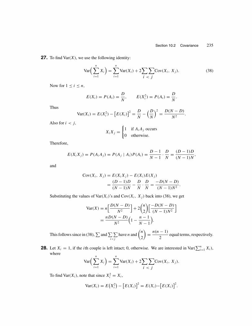
Section 10.2 Covariance 235
27. To find Var(X), we use the following identity:
Var( n∑
i=1
Xi
)=
n∑i=1
Var(Xi) + 2∑∑i < j
Cov(Xi, Xj ). (38)
Now for 1 ≤ i ≤ n,
E(Xi) = P(Ai) = D
N, E(X2
i ) = P(Ai) = D
N.
Thus
Var(Xi) = E(X2i ) − [
E(Xi)]2 = D
N−(D
N
)2 = D(N − D)
N2.
Also for i < j,
XiXj ={
1 if AiAj occurs
0 otherwise.
Therefore,
E(XiXj) = P(AiAj ) = P(Aj | Ai)P (Ai) = D − 1
N − 1· D
N= (D − 1)D
(N − 1)N,
and
Cov(Xi, Xj ) = E(XiXj) − E(Xi)E(Xj)
= (D − 1)D
(N − 1)N− D
N· D
N= −D(N − D)
(N − 1)N2.
Substituting the values of Var(Xi)’s and Cov(Xi, Xj ) back into (38), we get
Var(X) = n[D(N − D)
N2
]+ 2
(n
2
)[−D(N − D)
(N − 1)N2
]= nD(N − D)
N2
(1 − n − 1
N − 1
).
This follows since in (38),∑
and∑∑
i<j
have n and
(n
2
)= n(n − 1)
2equal terms, respectively.
28. Let Xi = 1, if the ith couple is left intact; 0, otherwise. We are interested in Var(∑n
i=1 Xi),where
Var( n∑
i=1
Xi
)=
n∑i=1
Var(Xi) + 2∑∑i < j
Cov(Xi, Xj ).
To find Var(Xi), note that since X2i = Xi ,
Var(Xi) = E(X2
i
)− [E(Xi)
]2 = E(Xi)−[E(Xi)
]2.

236 Chapter 10 More Expectations and Variances
By Example 10.3,
E(Xi) = (2n − m)(2n − m − 1)
2n(2n − 1).
So
Var(Xi) = (2n − m)(2n − m − 1)
2n(2n − 1)
[1 − (2n − m)(2n − m − 1)
2n(2n − 1)
].
To find Cov(Xi, Xj ), note that XiXj = 1 if the ith and j th couples are left intact; 0, otherwise.Now
Cov(Xi, Xj ) = E(XiXj) − E(Xi)E(Xj) = P(XiXj = 1) − E(Xi)E(Xj)
=
(2n − 4
m
)(
2n
m
) −[(2n − m)(2n − m − 1)
2n(2n − 1)
]2.
Therefore,
Cov(Xi, Xj ) = (2n − m)(2n − m − 1)(2n − m − 2)(2n − m − 3)
2n(2n − 1)(2n − 2)(2n − 3)
−[(2n − m)(2n − m − 1)
2n(2n − 1)
]2.
So
Var
( n∑i=1
Xi
)= n
(2n − m)(2n − m − 1)
2n(2n − 1)
[1 − (2n − m)(2n − m − 1)
2n(2n − 1)
]
+ 2n(n − 1)
2
[(2n − m)(2n − m − 1)(2n − m − 2)(2n − m − 3)
2n(2n − 1)(2n − 2)(2n − 3)
− (2n − m)2(2n − m − 1)2
4n2(2n − 1)2
]
= (2n − m)(2n − m − 1)
2(2n − 1)
[1 − (2n − m)(2n − m − 1)
2n(2n − 1)
]
+ (n − 1)
[(2n − m)(2n − m − 1)(2n − m − 2)(2n − m − 3)
2(2n − 1)(2n − 2)(2n − 3)
− (2n − m)2(2n − m − 1)2
4n(2n − 1)2
]

Section 10.3 Correlation 237
= (2n − m)(2n − m − 1)
2(2n − 1)
[1 − (2n − m)(2n − m − 1)
2n(2n − 1)
+ (n − 1)(2n − m − 2)(2n − m − 3)
(2n − 2)(2n − 3)
− (n − 1)(2n − m)(2n − m − 1)
2n(2n − 1)
]
= (2n − m)(2n − m − 1)
2(2n − 1)
[1 + (n − 1)(2n − m − 2)(2n − m − 3)
(2n − 2)(2n − 3)
− (2n − m)(2n − m − 1)
2(2n − 1)
].
10.3 CORRELATION
1. We have that Cov(X, Y ) = ρ(X, Y )σXσY = 3; thus
Var(2X − 4Y + 3) = Var(2X − 4Y ) = 4Var(X) + 16Var(Y ) − 16Cov(X, Y )
= 4(4) + 16(9) − 16(3) = 112.
2. By Exercise 23 of Section 8.2, X and Y are independent random variables.[This can also be
shown directly by verifying the relation f (x, y) = fX(x)fY (y).]
Hence Cov(X, Y ) = 0, andtherefore ρ(X, Y ) = 0.
3. Let X and Y be the lengths of the pieces obtained. Since Y = 1 − X, by Theorem 10.5,ρ(X, Y ) = −1. Since X and Y are uniform over (0, 1), σX = 1/
√12 and σY = 1/
√12.
Therefore,
Cov(X, Y ) = ρ(X, Y )σXσY = (−1)( 1√
12
)( 1√12
)= − 1
12.
4. If α1β1 = 0, both sides of the relation are 0 and the equality holds. If α1β1 �= 0, then
ρ(α1X + α2, β1Y + β2) = Cov(α1X + α2, β1Y + β2)
σα1X+α2 · σβ1Y+β2
= Cov(α1X, β1Y )
|α1|σX · |β1|σY
= α1β1Cov(X, Y )
|α1||β1|σXσY
= sgn(α1β1)ρ(X, Y ).
5. No, because for all random variables X and Y , −1 ≤ ρ(X, Y ) ≤ 1.

238 Chapter 10 More Expectations and Variances
6. By Exercise 6 of Section 10.2,
Cov(X + Y, X − Y ) = Var(X) − Var(Y ).
Since Cov(X, Y ) = 0,
σX+Y · σX−Y = √Var(X + Y ) · Var(X − Y )
=√[
Var(X) + Var(Y )][
Var(X) + Var(Y )]
= Var(X) + Var(Y ).
Therefore,
ρ(X + Y, X − Y ) = Cov(X + Y, X − Y )
σX+Y · σX−Y
= Var(X) − Var(Y )
Var(X) + Var(Y ).
7. Using integration by parts, we obtain
E(X) = 1
2
∫ π/2
0
∫ π/2
0x sin(x + y) dx dy = π
4,
E(X2) = 1
2
∫ π/2
0
∫ π/2
0x2 sin(x + y) dx dy = π2
8+ π
2− 2.
Hence
Var(X) =(π2
8+ π
2− 2
)− π2
16= π
2− 2 + π2
16.
By symmetry, E(Y ) = π
4and Var(Y ) = π
2− 2 + π2
16. Since
E(XY) = 1
2
∫ π/2
0
∫ π/2
0xy sin(x + y) dx dy = π
2− 1,
Cov(X, Y ) =(π
2− 1
)− π2
16. Therefore,
ρ(X, Y ) = Cov(X, Y )√Var(X) · √
Var(Y )= (π/2) − 1 − (π2/16)
(π/2) − 2 + (π2/16)= −0.245.
Since ρ(X, Y ) �= ±1, there is no linear relation between X and Y .

Section 10.4 Conditioning on Random Variables 239
10.4 CONDITIONING ON RANDOM VARIABLES
1. Let N be the number of tosses required; then
E(N) = E[E(N |X)
] = E(N | X = 0)P (X = 0) + E(N | X = 1)P (X = 1)
= [1 + E(N)
]1
2+(1
2· 1 + 1
2
[2 + E(N)
])1
2.
Solving this equation for E(N), we obtain E(N) = 5.
2. We have that
E[Y (t)
] = E[E[Y (t)|X]] = E
[Y (t) | X < t
]P(X < t) + E
[Y (t) | X ≥ t
]P(X ≥ t)
= E[aX − a
3(t − X)
]P(X < t) + E(at)P (X ≥ t)
= E(4a
3X − at
3
)P(X < t) + atP (X ≥ t)
=[4a
3
(11
2
)− at
3
]( t − 4
7 − 4
)+ at
(7 − t
3
)= 1
9a(22 − t)(t − 4) + 1
3at (7 − t).
To find the value of t that maximizes E[Y (t)
], we solve
d
dtE[Y (t)
] = 1
9a(−8t + 47) = 0 for
t . We get t = 47/8 = 5.875.
3. (a) Clearly,
E(Xn | Xn−1 = x) = x · x
b+ (x + 1) · b − x
b= 1 +
(1 − 1
b
)x.
This implies that
E(Xn|Xn−1) = 1 +(
1 − 1
b
)Xn−1.
Therefore,
E(Xn) = E[E(Xn|Xn−1)
] = 1 +(
1 − 1
b
)E(Xn−1). (39)
Now we use induction to prove that
E(Xn) = b − d(
1 − 1
b
)n
. (40)
For n = 1, (40) holds since
E(X1) = (b − d)b − d
b+ (b − d + 1)
d
b= b − d
(1 − 1
b
).

240 Chapter 10 More Expectations and Variances
Suppose that (40) is valid for n, we show that it is valid for n + 1 as well. By (39),
E(Xn+1) = 1 +(
1 − 1
b
)E(Xn) = 1 +
(1 − 1
b
)[b − d
(1 − 1
b
)n]= 1 + b
(1 − 1
b
)− d
(1 − 1
b
)n+1 = b − d(
1 − 1
b
)n+1.
This shows that (40) holds for n + 1, and hence for all n.
(b) We have that
P(En) =b∑
x=b−d
P (En | Xn−1 = x)P (Xn−1 = x) =b∑
x=b−d
x
bP (Xn−1 = x)
= 1
b
b∑x=b−d
xP (Xn−1 = x) = 1
bE(Xn−1) = 1 − d
b
(1 − 1
b
)n−1.
4. Let V be a random variable defined by
V ={
1 with probability p
0 with probability 1 − p.
Then
X ={
Y if V = 1
Z if V = 0.
Therefore,
E(X) = E[E(X | V )
] = E(X | V = 1)P (V = 1) + E(X | V = 0)P (V = 0)
= E(Y )p + E(Z)(1 − p).
5. The probability that a page should be retyped is
p = 1 − e−3/2(3/2)0
0! − e−3/2(3/2)1
1! − e−3/2(3/2)2
2! = 0.1912.
Thus E(X1) = 200(0.1912) and
E(X2) = E[E(X2|X1)
] =200∑x=0
E(X2 | X1 = x)P (X1 = x)
=200∑x=0
(0.1912)xP (X1 = x) = (0.1912)E(X1) = (0.1912)2(200).
Similarly,E(X3) = E
[E(X3|X2)
] = (0.1912)3(200)

Section 10.4 Conditioning on Random Variables 241
and, in general,
E(Xn) = (0.1912)n(200).
Therefore, by (10.2),
E( ∞∑
i=1
Xi
)=
∞∑i=1
E(Xi) =∞∑i=1
(0.1912)i(200) = 200( 0.1912
1 − 0.1912
)= 47.28.
6. For i ≥ 1, let Xi be the length of the ith character of the message. Since the total number ofthe bits of the message is
∑Ki=1 Xi , and since it will take (1/1000)th of a second to emit a bit,
we have that T = (1/1000)∑K
i=1 Xi . By Wald’s equation and Theorem 10.8,
E(T ) = 1
1000E(K)E(X1) = 1
1000µ · 1
p= µ
1000p
Var(T ) =( 1
1000
)2[E(K)Var(X1) + [
E(X1)]2
Var(K)]
=( 1
1000
)2[µ · 1 − p
p2+ 1
p2σ 2]
= µ(1 − p) + σ 2
1, 000, 000p2.
7. We have that
E(Xn) = E[E(Xn|Y )
] = E(Xn | Y = 1)P (Y = 1) + E(Xn | Y = 0)P (Y = 0)
= 0 · P(Y = 1) + [1 + E(Xn+1)
]39 − n
52 − n.
This recursive relation and E(X39) = 0 imply that E(X38) = 1/14, E(X37) = 2/14,E(X36) = 3/14, and, in general, E(Xi) = (39 − i)/14. The answer is
1 + E(X0) = 1 + 39
14= 53
14= 3.786.
8. Let F be the distribution function of X. We have
P(X < Y) =∫ ∞
−∞P(X < Y | Y = y)g(y) dy
=∫ ∞
−∞P(X < y) g(y) dy =
∫ ∞
−∞F(y) g(y) dy.

242 Chapter 10 More Expectations and Variances
9. Let f be the probability density function of λ; then
P(N = i) =∫ ∞
0P(N = i | λ = x)f (x) dx
=∫ ∞
0
e−xxi
i! e−x dx =∫ ∞
0
e−2xxi
i! dx
= 1
i!(1
2
)i∫ ∞
0e−2x(2x)i dx
= 1
i!(1
2
)i+1∫ ∞
0e−uui du =
(1
2
)i+1.
In these calculations, we have used the substitution u = 2x and the relation∫ ∞
0e−uui du = i!.
10. Suppose that player A carries x dollars in his wallet. Then player A wins if and only if playerB carries y dollars, y ∈ (x, 1] in his wallet. Thus player A wins y dollars with probability1−x. In such a case, the expected amount player A wins is (1+x)/2. Player A loses x dollarswith probability x. Therefore,
E(WA | X = x) = 1 + x
2· (1 − x) + (−x) · x = 1
2− 3
2x2.
Let fX be the probability density function of X, then
fX(x) ={
1 if 0 ≤ x ≤ 1
0 otherwise.
Therefore,
E(WA) = E[E(WA | X)
] =∫ 1
0E(WA | X = x)fX(x) dx
=∫ 1
0
(1
2− 3
2x2)
dx =[1
2x − 1
2x3]1
0= 0.
The solution above was presented by Kent G. Merryfield, Ngo Viet, and Saleem Watson intheir joint paper "The Wallet Paradox" published in the August-September 1977 issue of theAmerican Mathematical Monthly. Note the following observations by the authors.
It is interesting to consider special cases of this formula for the conditional expec-tation. Since E(WA | X = 1) = −1 and E(WA | X = 0) = 1/2, we see that a playercarrying one dollar in his wallet should expect to lose it, whereas a player carryingnothing in his wallet should expect to gain half a dollar (the mean). Interestingly, if aplayer is carrying half a dollar (the mean) in his wallet, then E(WA | X = 1/2) = 1/8;that is, his expectation of winning is positive.
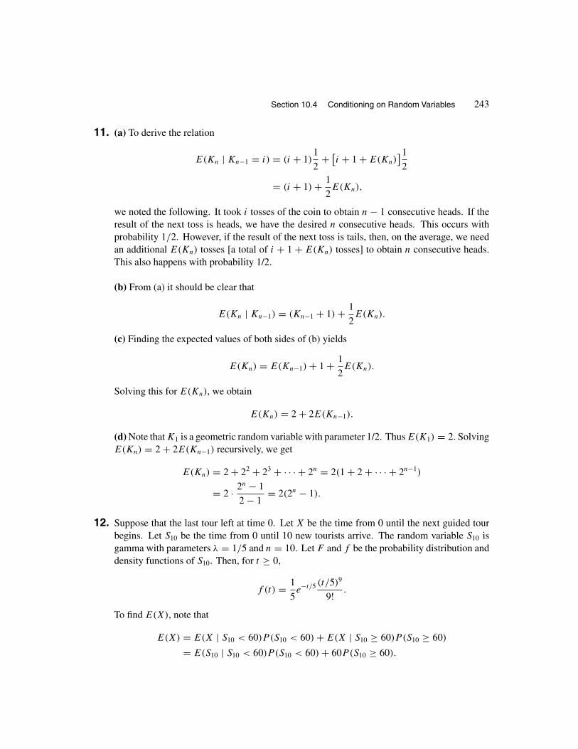
Section 10.4 Conditioning on Random Variables 243
11. (a) To derive the relation
E(Kn | Kn−1 = i) = (i + 1)1
2+ [
i + 1 + E(Kn)]1
2
= (i + 1) + 1
2E(Kn),
we noted the following. It took i tosses of the coin to obtain n − 1 consecutive heads. If theresult of the next toss is heads, we have the desired n consecutive heads. This occurs withprobability 1/2. However, if the result of the next toss is tails, then, on the average, we needan additional E(Kn) tosses [a total of i + 1 + E(Kn) tosses] to obtain n consecutive heads.This also happens with probability 1/2.
(b) From (a) it should be clear that
E(Kn | Kn−1) = (Kn−1 + 1) + 1
2E(Kn).
(c) Finding the expected values of both sides of (b) yields
E(Kn) = E(Kn−1) + 1 + 1
2E(Kn).
Solving this for E(Kn), we obtain
E(Kn) = 2 + 2E(Kn−1).
(d) Note that K1 is a geometric random variable with parameter 1/2. Thus E(K1) = 2. SolvingE(Kn) = 2 + 2E(Kn−1) recursively, we get
E(Kn) = 2 + 22 + 23 + · · · + 2n = 2(1 + 2 + · · · + 2n−1)
= 2 · 2n − 1
2 − 1= 2(2n − 1).
12. Suppose that the last tour left at time 0. Let X be the time from 0 until the next guided tourbegins. Let S10 be the time from 0 until 10 new tourists arrive. The random variable S10 isgamma with parameters λ = 1/5 and n = 10. Let F and f be the probability distribution anddensity functions of S10. Then, for t ≥ 0,
f (t) = 1
5e−t/5 (t/5)9
9! .
To find E(X), note that
E(X) = E(X | S10 < 60)P (S10 < 60) + E(X | S10 ≥ 60)P (S10 ≥ 60)
= E(S10 | S10 < 60)P (S10 < 60) + 60P(S10 ≥ 60).

244 Chapter 10 More Expectations and Variances
Now
P(S10 < 60) =∫ 60
0
1
5e−t/5 (t/5)9
9! dt = 0.7576,
and, by Remark 8.1,
E(S10 | S10 < 60) = 1
F(60)
∫ 60
0tf (t) dt
= 1
0.7576
∫ 60
0
1
5te−t/5 (t/5)9
9! dt = 43.0815.
Therefore,E(X) = (43.0815)(0.7576) + 60(1 − 0.7576) = 47.18.
This shows that the expected length of time between two consecutive tours is approximately47 minutes and 10 seconds.
13. Let X1 be the time until the first application arrives. Let X2 be the time between the first andsecond applications, and so forth. Then Xi’s are independent exponential random variableswith mean 1/λ = 1/5 of a day. Let N be the first integer for which
X1 ≤ 2, X2 ≤ 2, . . . , XN ≤ 2, XN+1 > 2.
The time that the admissions office has to wait before doubling its student recruitment effortsis SN+1 = X1 + X2 + · · · + XN+1. Therefore,
E(SN+1) = E[E(SN+1 | N)
] =∞∑i=0
E(SN+1 | N = i)P (N = i).
Now, for i ≥ 0,
E(SN+1 | N = i) = E(X1 + X2 + · · · + Xi+1 | N = i) =i+1∑j=1
E(Xj | N = i)
=[ i∑
j=1
E(Xj | Xj ≤ 2)]
+ E(Xi+1 | Xi+1 > 2),
where by Remark 8.1,
E(Xj | Xj ≤ 2) = 1
F(2)
∫ 2
0tf (t) dt,
E(Xi+1 | Xi+1 > 2) = 1
1 − F(2)
∫ ∞
2tf (t) dt,

Section 10.4 Conditioning on Random Variables 245
F and f being the probability distribution and density functions of Xi’s, respectively. That is,for t ≥ 0, F(t) = 1 − e−5t , f (t) = 5e−5t . Thus, for 1 ≤ j ≤ i,
E(Xj | Xj ≤ 2) = 1
1 − e−10
∫ 2
05t e−5t dt = (1.0000454)
[(− t − 1
5
)e−5t
]2
0
= (1.0000454)(0.19999) = 0.1999092
and, for j = i + 1,
E(Xi+1 | Xi+1 > 2) = 1
e−10
∫ ∞
25t e−5t dt = e10
[(− t − 1
5
)e−5t
]∞2
= 2.2.
Thus, for i ≥ 0,E(SN+1 | N = i) = (0.1999092)i + 2.2.
To find P(N = i), note that for i ≥ 0,
P(N = i) = P(X1 ≤ 2, X2 ≤ 2, . . . , Xi ≤ 2, Xi+1 > 2)
= [F(2)
]i[1 − F(2)
] = (0.9999546)i(0.0000454).
Putting all these together, we obtain
E(SN+1) =∞∑i=0
E(SN+1 | N = i)P (N = i)
=∞∑i=0
[(0.1999092)i + 2.2
](0.9999546)i(0.0000454)
= (0.00000908)
∞∑i=0
i(0.9999546)i + (0.00009988)
∞∑i=0
(0.9999546)i
= (0.00000908) · 0.9999546
(1 − 0.9999546)2+ (0.00009988) · 1
1 − 0.9999546
= 4407.286,
where the next to last equality follows from∑∞
i=1 iri = r/(1 − r)2, and∑∞
i=0 ri =1/(1 − r), |r| < 1. Since an academic year is 9 months long, and contains approximately180 business days, the admission officers should not be concerned about this rule at all. Itwill take 4,407.286 business days, on average, until there is a lapse of two days between twoconsecutive applications.
14. Let Xi be the number of calls until Steven has not missed Adam in exactly i consecutive calls.We have that
E(Xi | Xi−1
) ={
Xi−1 + 1 with probability p
Xi−1 + 1 + E(Xi) with probability 1 − p.
246 Chapter 10 More Expectations and Variances
Therefore,
E(Xi) = E[E(Xi | Xi−1)
] = [E(Xi−1) + 1
]p + [
E(Xi−1) + 1 + E(Xi)](1 − p).
Solving this equation for E(Xi), we obtain
E(Xi) = 1
p
[1 + E(Xi−1)
].
Now X1 is a geometric random variable with parameter p. So E(X1) = 1/p. Thus
E(X2) = 1
p
[1 + E(X1)
] = 1
p
(1 + 1
p
),
E(X3) = 1
p
[1 + E(X2)
] = 1
p
(1 + 1
p+ 1
p 2
),
...
E(Xk) = 1
p
(1 + 1
p+ 1
p 2+ · · · + 1
p k−1
)= 1
p· (1/p k) − 1
(1/p) − 1= 1 − p k
p k(1 − p).
15. Let N be the number of games to be played until Emily wins two of the most recent threegames. Let X be the number of games to be played until Emily wins a game for the first time.The random variable X is geometric with parameter 0.35. Hence E(X) = 1/0.35. First, wefind the random variable E(N | X) in terms of X. Then we obtain E(N) by calculating theexpected value of E(N | X). Let W be the event that Emily wins the (X + 1)st game as well.Let LW be the event that Emily loses the (X + 1)st game but wins the (X + 2)nd game. LetLL be the event that Emily loses both the (X + 1)st and the (X + 2)nd games. Given X = x,we have
E(N | X = x) = (x + 1)P (W) + (x + 2)P (LW) + [(x + 2) + E(N)
]P(LL).
So
E(N | X = x) = (x + 1)(0.35) + (x + 2)(0.65)(0.35) + [(x + 2) + E(N)
](0.65)2.
This givesE(N | X = x) = x + (0.4225)E(N) + 1.65.
Therefore,E(N | X) = X + (0.4225)E(N) + 1.65.
Hence
E(N) = E[E(N | X)
] = E(X) + (0.4225)E(N) + 1.65 = 1
0.35+ (0.4225)E(N) + 1.65.
Solving this for E(N) gives E(N) = 7.805.
Section 10.4 Conditioning on Random Variables 247
16. Since hemophilia is a sex-linked disease, and John is phenotypically normal, John is H .Therefore, no matter what Kim’s genotype is, none of the daughters has hemophilia. Whethera boy has hemophilia or not depends solely on the genotype of Kim. Let X be the numberof the boys who have hemophilia. To find, E(X), the expected number of the boys who havehemophilia, let
Z =
⎧⎪⎪⎨⎪⎪⎩0 if Kim is hh
1 if Kim is Hh
2 if Kim is HH .
Then
E(X) = E[E(X | Z)
]= E(X | Z = 0)P (Z = 0) + E(X | Z = 1)P (Z = 1) + E(X | Z = 2)P (Z = 2)
= 4(0.02)(0.02) + 4(1/2)[2(0.98)(0.02)
]+ 0[0.98)(0.98)
] = 0.08.
Therefore, on average, 0.08 of the boys and hence 0.08 of the children are expected to havehemophilia.
17. Let X be the number of bags inspected until an unacceptable bag is found. Let Kn be the numberof consequent bags inspected until n consecutive acceptable bags are found. The number ofbags inspected in one inspection cycle is X + Km. We are interested in E(X + Km) =E(X) + E(Km). Clearly, X is a geometric random variable with parameter α(1 − p). SoE(X) = 1/
[α(1 − p)
]. To find E(Km), note that ∀n,
E(Kn) = E[E(Kn | Kn−1)
].
Now
E(Kn | Kn−1 = i) = (i + 1)p + [i + 1 + E(Kn)
](1 − p)
= (i + 1) + (1 − p)E(Kn). (41)
To derive this relation, we noted the following. It took i inspections to find n − 1 consecutiveacceptable bags. If the next bag inspected is also acceptable, we have the n consecutiveacceptable bags required in i + 1 inspections. This occurs with probability p. However, ifthe next bag inspected is unacceptable, then, on the average, we need an additional E(Kn)
inspections[a total of i + 1 + E(Kn) inspections
]until we get n consecutive acceptable bags
of cinnamon. This happens with probability 1 − p.
From (41), we have
E(Kn | Kn−1) = (Kn−1 + 1) + (1 − p)E(Kn).
Finding the expected values of both sides of this relation gives
E(Kn) = E(Kn−1) + 1 + (1 − p)E(Kn).

248 Chapter 10 More Expectations and Variances
Solving for E(Kn), we obtain
E(Kn) = 1
p+ E(Kn−1)
p.
Noting that E(K1) = 1/p and solving recursively, we find that
E(Kn) = 1
p+ 1
p2+ · · · + 1
pn.
Therefore, the desired quantity is
E(X + Km) = E(X) + E(Km)
= 1
α(1 − p)+ 1
p
(1 + 1
p+ · · · + 1
pm−1
)
= 1
α(1 − p)+ 1
p·
( 1
p
)m − 1
1
p− 1
= (1 − α)pm + α
αpm(1 − p).
18. For 0 < t ≤ 1, let N(t) be the number of batteries changed by time t . Let X be the lifetimeof the initial battery used; X is a uniform random variable over the interval (0, 1). Therefore,fX, the probability density function of X, is given by
fX(x) ={
1 if 0 < x < 1
0 otherwise.
We are interested in K(t) = E[N(t)
]. Clearly,
E[N(t)
] = E[E[N(t) | X
]] =∫ ∞
0E[N(t) | X = x
]fX(x) dx
=∫ t
0
[1 + E
[N(t − x)
]]dx = t +
∫ t
0E[N(t − x)
]dx
= t +∫ t
0K(u) du,
where the last equality follows from the substitution u = t − x. Differentiating both sides ofK(t) = t + ∫ t
0 K(u) du with respect to t , we obtain K′(t) = 1 + K(t) which is equivalent to
K′(t)
1 + K(t)= 1.
Thus, for some constant c,ln[1 + K(t)
] = t + c,

Section 10.4 Conditioning on Random Variables 249
or,1 + K(t) = et+c.
The initial condition K(0) = E[N(0)
] = 0 yields ec = 1; so
K(t) = et − 1.
On average, after 950 hours of operation, K(0.95) = 1.586 batteries are used.
19. Since E(X|Y ) is a function of Y , by Example 10.23,
E(XZ) = E[E(XZ|Y )
] = E[E[XE(X|Y )|Y ]]
= E[E(X|Y )E(X|Y )
] = E(Z2).
Therefore,
E[(
X − E(X|Y ))2]
= E[(X − Z)2
]= E(X2 − 2ZX + Z2) = E(X2) − 2E(Z2) + E(Z2)
= E(X2) − E(Z2) = E(X2) − E[E(X|Y )2
].
20. Let Z = E(X|Y ); then
Var(X|Y ) = E[(X − Z)2|Y ]
= E(X2 − 2XZ + Z2|Y )
= E(X2|Y ) − 2E(XZ|Y ) + E(Z2|Y ).
Since E(X|Y ) is a function of Y , by Example 10.23,
E(XZ|Y ) = E[XE(X|Y )|Y ] = E(X|Y )E(X|Y ) = Z2.
AlsoE(Z2|Y ) = E
[E(X|Y )2|Y ] = E(X|Y )2 = Z2
since, in general, E[f (Y )|Y ] = f (Y ): if Y = y, then E
[f (Y )|Y ] is defined to be
E[f (Y )|Y = y
] = E[f (y)|Y = y
] = f (y).
Therefore,Var(X|Y ) = E(X2|Y ) − 2Z2 + Z2 = E(X2|Y ) − E(X|Y )2.
21. By the definition of variance,
Var( N∑
i=1
Xi
)= E
[( N∑i=1
Xi
)2]−[E( N∑
i=1
Xi
)]2, (42)

250 Chapter 10 More Expectations and Variances
where by Wald’s equation,
[E( N∑
i=1
Xi
)]2 = [E(X)E(N)
]2 = [E(N)
]2 · [E(X)]2
. (43)
Now since N is independent of {X1, X2, . . . },
E[( N∑
i=1
Xi
)2] = E[E( N∑
i=1
Xi
)2 ∣∣∣ N]
=∞∑
n=1
E[( N∑
i=1
Xi
)2 ∣∣∣ N = n]P(N = n)
=∞∑
n=1
E[( n∑
i=1
Xi
)2 ∣∣∣ N = n]P(N = n)
=∞∑
n=1
E( n∑
i=1
Xi
)2P(N = n).
Thus
E[( N∑
i=1
Xi
)2] =∞∑
n=1
E( n∑
i=1
X2i + 2
∑∑i<j
XiXj
)P(N = n)
=∞∑
n=1
[nE(X2) + 2
∑∑i<j
E(Xi)E(Xj)]P(N = n)
= E(X2)
∞∑n=1
nP (N = n) +∞∑
n=1
2
(n
2
)E(X)E(X)P (N = n) =
= E(X2)E(N) + [E(X)
]2∞∑
n=1
n(n − 1)P (N = n)
= E(X2)E(N) + [E(X)
]2E[N(N − 1)
]= E(X2)E(N) + [
E(X)]2
E(N2) − [E(X)
]2E(N).
Putting this and (43) in (42), we obtain
Var( N∑
i=1
Xi
)= E(X2)E(N) + [
E(X)]2
E(N2) − [E(X)
]2E(N) − [
E(N)]2[
E(X)]2
= E(N)(E(X2) − [
E(X)]2)
+ [E(X)
]2(E(N2) − [
E(N)]2).

Section 10.5 Bivariate Normal Distribution 251
Therefore,
Var( N∑
i=1
Xi
)= E(N)Var(X) + [E(X)]2Var(N).
10.5 BIVARIATE NORMAL DISTRIBUTION
1. The conditional probability density function of Y , given that X = 70 is normal with mean
E(Y | X = x) = µY + ρσY
σX
(x − µX) = 60 + (0.45)(2.7
3
)(70 − 71) = 59.595,
and standard deviation
σ 2Y |X=x =
√(1 − ρ 2)σ 2
Y = 2.7√
1 − (0.45)2 = 2.411.
Therefore, the desired probability is
P(Y ≥ 59 | X = 70) = P(Y − 59.595
2.411≥ 59 − 59.595
2.411
∣∣∣∣X = 70)
= 1 − �(−0.25) = �(0.25) = 0.5987.
2. By (10.24),
f (x, y) = 1
162πexp
[ 1
162
(x2 + y2
)].
(a) Since ρ = 0, X and Y are independent normal random variables with mean 0 and standarddeviation 9. Therefore,
P(X ≤ 6, Y ≤ 12
) = P(X ≤ 6)P (Y ≤ 12) = P(X − 0
9≤ 6
9
)P(Y − 0
12≤ 12
9
)= �(0.67)�(1.23) = (0.7486)(0.9082) = 0.68.
(b) To find P(X2 + Y 2 ≤ 36
), we use polar coordinates.
P(X2 + Y 2 ≤ 36
) = 1
162π
∫∫x2+y2≤36
exp[
− 1
162
(x2 + y2
)]dy dx
= 1
2π
∫ 2π
0
∫ 6
0exp
(− 1
162r2)
· 2r
162dr dθ.
Now let u = r2/162; du = (2r/162)dr and we get
P(X2 + Y 2 ≤ 36
) = 1
2π
∫ 2π
0
(∫ 2/9
0e−u du
)dθ = 1 − e−2/9 = 0.8.

252 Chapter 10 More Expectations and Variances
3. Note thatVar(αX + Y ) = α2σ 2
X + σ 2Y + 2αρ(X, Y )σXσY .
Settingd
dαVar(αX + Y ) = 0, we get α = −ρ(X, Y )
σY
σX
.
4. By (10.24), f (x, y) is maximum if and only if Q(x, y) is minimum. Let z1 = x − µX
σX
and
z2 = y − µY
σY
. Then |ρ| ≤ 1 implies that
Q(x, y) = z21 − 2ρz1z2 + z2
2 ≥ z21 − 2|ρz1z2| + z2
2
≥ z21 − 2|z1z2| + z2
2 = (|z1| − |z2|)2 ≥ 0.
This inequality shows that Q is minimum if Q(x, y) = 0. This happens at x = µX andy = µY . Therefore, (µX, µY ) is the point at which the maximum of f is obtained.
5. We have that
fX(x) =∫ x
02 dy = 2x, 0 < x < 1,
fY (y) =∫ 1
y
2 dx = 2(1 − y), 0 < y < 1,
fX|Y (x|y) = 2
2(1 − y)= 1
1 − y, y < x < 1.
fY |X(y|x) = 2
2x= 1
x, 0 < y < x.
Therefore,
E(X | Y = y) =∫ 1
y
xfX|Y (x|y) dx =∫ 1
y
x1
1 − ydx = 1 + y
2, 0 < y < 1,
E(Y | X = x) =∫ x
0yfY |X(y|x) dy =
∫ x
0y
1
xdy = x
2, 0 < x < 1.
Now since E(Y | X = x) is a linear function of x and E(X | Y = y) is a linear function of y,by Lemma 10.3,
µY + ρσY
σX
(x − µX) = x
2

Section 10.5 Bivariate Normal Distribution 253
and
µX + ρσX
σY
(y − µY ) = 1 + y
2.
These relations imply that
ρσY
σX
= 1
2and ρ
σX
σY
= 1
2.
Hence ρ > 0 and ρ 2 = ρσY
σX
· ρσX
σY
= 1
4. Therefore ρ = 1/2.
6. We use Theorem 8.8 to find the joint probability density function of X and Y . The jointprobability density function of Z and W is given by
f (z, w) = 1
2πexp
[− 1
2
(z2 + w2
)].
Let h1(z, w) = σ1z+µ1 and h2(z, w) = σ2(ρz+√1 − ρ 2 w
)+µ2. The system of equations⎧⎨⎩σ1z + µ1 = x
σ2(ρz +√
1 − ρ 2 w)+ µ2 = y
defines a one-to-one transformation of R2 in the zw-plane onto R2 in the xy-plane. It has aunique solution
z = x − µ1
σ1,
w = 1√1 − ρ 2
[y − µ2
σ2− ρ(x − µ1)
σ1
]for z and w in terms of x and y. Moreover,
J =
∣∣∣∣∣∣∣∣∣∣
1
σ10
− ρ
σ1
√1 − ρ 2
1
σ2
√1 − ρ 2
∣∣∣∣∣∣∣∣∣∣= 1
σ1σ2
√1 − ρ 2
�= 0.
Hence, by Theorem 8.8, the joint probability density function of X and Y is given by
1
σ1σ2
√1 − ρ 2
f(x − µ1
σ1,
1√1 − ρ 2
[y − µ2
σ2− ρ
x − µ1
σ1
]).
Noting that f (z, w) = 1
2πexp
[− 1
2
(z2 + w2
)]. Straightforward calculations will result in
(10.24), showing that the joint probability density function of X and Y is bivariate normal.

254 Chapter 10 More Expectations and Variances
7. Using Theorem 8.8, it is straightforward to show that the joint probability density function ofX + Y and X − Y is bivariate normal. Since
ρ(X + Y, X − Y ) = Cov(X + Y, X − Y )
σX+Y · σX−Y
= Var(X) − Var(Y )
σX+Y · σX−Y
= 0,
X + Y and X − Y are uncorrelated. But for bivariate normal, uncorrelated and independenceare equivalent. So X + Y and X − Y are independent.
REVIEW PROBLEMS FOR CHAPTER 10
1. Number the last 10 graduates who will walk on the stage 1 through 10. Let Xi = 1 if the ithgraduate receives his or her own diploma; 0, otherwise. The number of graduates who willreceive their own diploma is X = X1 + X2 + · · · + Xn. Since
E(Xi) = 1 · 1
n+ 0 ·
(1 − 1
n
)= 1
n,
we have
E(X) = E(X1) + E(X2) + · · · + E(Xn) = n · 1
n= 1.
2. Since
E(X) =∫ 2
1(2x2 − 2x) dx = 5
3,
and
E(X3) =∫ 2
1(2x4 − 2x3) dx = 49
10,
we have that
E(X3 + 2X − 7) = 49
10+ 10
3− 7 = 37
30.
3. Since
E(X2) = 1
3
∫ 1
0
∫ 2
0(3x5 + x3y) dy dx = 1
2,
and
E(XY) = 1
3
∫ 1
0
∫ 2
0(3x4y + x2y2) dy dx = 94
135,
we have that E(X2 + 2XY) = 1
2+ 188
135= 511
270.

Chapter 10 Review Problems 255
4. Let X1, X2, . . . , Xn be geometric random variables with parameters 1, (n − 1)/n, (n − 2)/n,. . . , 1/n, respectively. The desired quantity is
E(X1 + X2 + · · · + Xn) = 1 + n
n − 1+ n
n − 2+ · · · + n
= 1 + n( 1
n − 1+ 1
n − 2+ · · · + 1
2+ 1
)= 1 + nan−1.
5. Let X be the number of tosses until 4 consecutive sixes. Let Y be the number of tosses untilthe first non-six outcome is obtained. We have
E(X) = E[E(X|Y )
] =∞∑i=1
E(X | Y = i)P (Y = i)
=4∑
i=1
E(X | Y = i)P (Y = i) +∞∑i=5
E(X | Y = i)P (Y = i)
=4∑
i=1
[i + E(X)
](1
6
)i−1(5
6
)+
∞∑i=5
4(1
6
)i−1(5
6
).
This equation reduces to
E(X) = [1 + E(X)
]5
6+ [
2 + E(X)]1
6· 5
6+ [
3 + E(X)](1
6
)2(5
6
)+ [
4 + E(X)](1
6
)3(5
6
)+ 4
(5
6
) (1/6)4
1 − (1/6).
Solving this equation for E(X), we obtain E(X) = 1554.
6. f (x, y, z) = (2x)(2y)(2z), 0 < x < 1, 0 < y < 1, 0 < z < 1. Since 2x, 0 < x < 1is a probability density function, 2y, 0 < y < 1 is a probability density function, and 2z,0 < z < 1 is also a probability density function, these three functions are fX(x), fY (y), andfZ(z), respectively. Therefore, f (x, y, z) = fX(x)fY (y)fZ(z) showing that X, Y , and Z areindependent. Thus
ρ(X, Y ) = ρ(Y, Z) = ρ(X, Z) = 0.
7. Since Cov(X, Y ) = σXσY ρ(X, Y ) = 2,
Var(3X − 5Y + 7) = Var(3X − 5Y ) = 9Var(X) + 25Var(Y ) − 15Cov(X, Y )
= 9 + 225 − 30 = 204.
8. Clearly,
pX(1) = p(1, 1) + p(1, 3) = 12/25, pX(2) = p(2, 3) = 13/25;pY (1) = p(1, 1) = 2/25, pY (3) = p(1, 3) + p(2, 3) = 23/25.

256 Chapter 10 More Expectations and Variances
Therefore,
pX(x) =⎧⎨⎩12/25 if x = 1
13/25 if x = 2,pY (y) =
⎧⎨⎩2/25 if y = 1
23/25 if y = 3.
These yield
E(X) = 1 · 12
25+ 2 · 13
25= 38
25;
E(Y ) = 1 · 2
25+ 3 · 23
25= 71
25;
E(XY) = (1)(1)1
25(12 + 12) + (1)(3)
1
25(12 + 32) + (2)(3)
1
25(22 + 32) = 22
5.
Thus
Cov(X, Y ) = E(XY) − E(X)E(Y ) = 22
5− 38
25· 71
25= 52
625.
9. In Exercise 6, Section 8.1, we calculated p(x, y), pX(x), and pY (y). The results of thatexercise yield
E(X) =12∑
x=2
xpX(x) = 7;
E(Y ) =5∑
y=0
ypY (y) = 35/18;
E(XY) =12∑
x=2
5∑y=0
xyp(x, y) = 245/18.
Therefore,
Cov(X, Y ) = E(XY) − E(X)E(Y ) = (245/18) − 7(35/18) = 0.
This shows that X and Y are uncorrelated. Note that X and Y are not independent as thefollowing shows.
1/36 = p(2, 0) �= pX(2)pY (0) = (1/36)(6/36) = 1/216.
10. Let p be the probability mass function of |X−Y |, q be the probability mass function of X+Y ,and r be the probability mass function of |X2 − Y 2|. We have
x 0 1 2p(x) 726/1296 520/1296 50/1296,

Chapter 10 Review Problems 257
x 0 1 2 3 4q(x) 625/1296 500/1296 150/1296 20/1296 1/1296,
x 0 1 3 4r(x) 726/1296 500/1296 20/1296 50/1296.
Using these we obtain
E(|X2 − Y 2|) = 760
1296, E
(|X − Y |) = 620
1296, E(X + Y ) = 864
1296,
E(|X − Y |2) = 720
1296, E
[(X + Y )2
] = 1, σ|X−Y | = 0.572,
σX+Y = 0.831.
Therefore,
ρ(|X − Y |, |X + Y |) = Cov
(|X − Y |, X + Y)
σ|X−Y | · σX+Y
= E(|X2 − Y 2|)− E
(|X − Y |)E(X + Y )
σ|X−Y | · σX+Y
= (760/1296) − (620/1296)(864/1296)
(0.831)(0.572)= 0.563.
11. One way to solve this problem is to note that the desired probability is the area of the regionunder the curve y = sin x from x = 0 to x = π/2 divided by the area of the rectangle[0, π/2] × [0, 1]. Hence it is ∫ π/2
0sin x dx
π/2= 2
π.
A second way to find this probability is to note that (X, Y ) lies below the curve y = sin x ifand only if Y < sin X. Noting that f , the probability density function of X is given by
f (x) =
⎧⎪⎨⎪⎩2
πif 0 < x <
π
2
0 otherwise,
and conditioning on X, we obtain
P(Y < sin X) =∫ π/2
0P(Y < sin X | X = x)f (x)dx =
∫ π/2
0
sin x − 0
1 − 0· 2
πdx
= − 2
πcos x
∣∣∣∣π/2
0
= 2
π.

258 Chapter 10 More Expectations and Variances
12. (a) Clearly,
fX(x) =∫ x
0e−x dy = xe−x, 0 < x < ∞,
fY (y) =∫ ∞
y
e−x dx = e−y, 0 < y < ∞.
(b) we have that
E(X) =∫ ∞
0x2e−x = 2, E(Y ) =
∫ ∞
0ye−y = 1,
E(X2) =
∫ ∞
0x3e−x dx = 6, E
(Y 2) =
∫ ∞
0y2e−y = 2.
Therefore, Var(X) = 2 and Var(Y ) = 1. Also
E(XY) =∫ ∞
0
∫ ∞
y
e−x dx dy = 3.
Thus
ρ(X, Y ) = E(XY) − E(X)E(Y )
σXσY
= 3 − 2√2 · 1
= 1√2.
13. Let h(α, β) = E[(Y − α − βX)2
]. Then
h(α, β) = E(Y 2)+ α2 + β2E
(X2)− 2αE(Y ) − 2βE(XY) + 2αβE(X).
Setting∂h
∂α= 0 and
∂h
∂β= 0, we obtain
{α + E(X)β = E(Y )
E(X)α + E(X2)β = E(XY).
Solving this system of two equations in two unknowns, we obtain
β = Cov(X, Y )
σ 2X
= ρσXσY
σ 2X
= ρσY
σX
,
α = µY − ρσY
σX
µX.
Therefore, Y = µY + ρσY
σX
(X − µX).
14. We have that
E(X) =∫ ∞
0
∫ ∞
0xye−y(1+x) dy dx =
∫ ∞
0
x
1 + x
(∫ ∞
0(1 + x)ye−y(1+x) dy
)dx.

Chapter 10 Review Problems 259
Now∫∞
0 (1 + x)ye−y(1+x) dy is the expected value of an exponential random variable withparameter 1 + x, so it is 1/(1 + x). Letting u = 1 + x, we have
E(X) =∫ ∞
0
x
(1 + x)2dx =
∫ ∞
1
u − 1
u2du
=∫ ∞
1
1
udu −
∫ ∞
1
1
u2du = ln u
∣∣∣∣∞1
− 1 = ∞.
(b) To find E(X|Y ), note that
E(X | Y = y) =∫ ∞
0xfX|Y (x|y) dx =
∫ ∞
0x
f (x, y)
fY (y)dx,
where
fY (y) =∫ ∞
0ye−y(1+x) dx = e−y
∫ ∞
0ye−yx dx = e−y.
Note that∫∞
0 ye−yx dx = 1 because ye−yx is the probability density function of an exponentialrandom variable with parameter 1. So
E(X | Y = y) =∫ ∞
0x
ye−ye−yx
e−ydx =
∫ ∞
0xye−xy dx = 1
y,
where the last equality holds because the last integral is the expected value of an exponentialrandom variable with parameter y. Since ∀y > 0, E(X | Y = y) = 1/y, E(X|Y ) = 1/Y.
15. Let X and Y denote the number of minutes past 10:00 A.M. that bus A and bus B arrive atthe station, respectively. X is uniformly distributed over (0, 30). Given that X = x, Y isuniformly distributed over (0, x). Let f (x, y) be the joint probability density function of X
and Y . We calculate E(Y ) by conditioning on X:
E(Y ) = E[E(Y |X)
] =∫ ∞
−∞E(Y | X = x)fX(x) dx =
∫ 30
0
x
2· 1
30dx = 30
4.
Thus the expected arrival time of bus B is 7.5 minutes past 10:00 A.M.
16. To find the distribution function of∑N
i=1 Xi , note that
P( N∑
i=1
Xi ≤ t)
=∞∑
n=1
P( N∑
i=1
Xi ≤ t∣∣N = n
)P(N = n)
=∞∑
n=1
P( n∑
i=1
Xi ≤ t∣∣N = n
)P(N = n)
=∞∑
n=1
P( n∑
i=1
Xi ≤ t)P(N = n),

260 Chapter 10 More Expectations and Variances
where the last inequality follows since N is independent of{X1, X2, X3, . . .
}. Now
∑ni=1 Xi
is a gamma random variable with parameters n and λ. Thus
P( N∑
i=1
Xi ≤ t)
=∞∑
n=1
[∫ t
0λe−λx (λx)n−1
(n − 1)! dx
](1 − p)n−1p
=∞∑
n=1
∫ t
0λpe−λx
[λ(1 − p)x
]n−1
(n − 1)! dx
=∫ t
0λpe−λx
∞∑n=1
[λ(1 − p)x
]n−1
(n − 1)! dx
=∫ t
0λpe−λxeλ(1−p)x dx
=∫ t
0λpe−λpx dx = 1 − e−λpt .
This shows that∑N
i=1 Xi is exponential with parameter λp.
17. Let X1, X2, . . . , Xi , . . . , X20 be geometric random variables with parameters 1, 19/20, . . . ,[20 − (i − 1)
]/20, . . . , 1/20. The desired quantity is
E( 20∑
i=1
Xi
)=
20∑i=1
E(Xi) =20∑i=1
20
20 − (i − 1)= 71.9548.

Chapter 11
Sums of Independent
Random Variables
and Limit Theorems
11.1 MOMENT-GENERATING FUNCTIONS
1. MX(t) = E(etX) =
5∑x=1
etxp(x) = 1
5
(et + e2t + e3t + e4t + e5t
).
2. (a) For t �= 0,
MX(t) = E(etX) =
∫ 3
−1
1
4etx dx = 1
4
(e3t − e−t
t
),
whereas for t = 0, MX(0) = 1. Thus
MX(t) =
⎧⎪⎨⎪⎩1
4
(e3t − e−t
t
)if t �= 0
1 if t = 0.
Since X is uniform over (−1, 3), E(X) = −1 + 3
2= 1 and Var(X) =
[3 − (−1)
]2
12= 4
3.
(b) By the definition of derivative,
E(X) = M ′X(0) = lim
h→0
MX(h) − MX(0)
h= lim
h→0
1
h
(e3h − e−h
4h− 1
)
= limh→0
e3h − e−h − 4h
4h2= lim
h→0
3e3h + e−h − 4
8h= lim
h→0
9e3h − e−h
8= 1,
where the fifth and sixth equalities follow from L’Hôpital’s rule.

262 Chapter 11 Sums of Independent Random Variables and Limit Theorems
3. Note that
MX(t) = E(etX) =
∞∑x=1
etx · 2(1
3
)x = 2∞∑
x=1
etx · e−x ln 3 = 2∞∑
x=1
ex(t−ln 3).
Restricting the domain of MX(t) to the set{t : t < ln 3
}and using the geometric series
theorem, we get
MX(t) = 2( et−ln 3
1 − et−ln 3
)= 2et
3 − et.
(Note that e− ln 3 = 1/3.) Differentiating MX(t), we obtain
M ′X(t) = 6et(
3 − et)2 ,
which gives E(X) = M ′X(0) = 3/2.
4. For t = 0, MX(0) = 1. For t �= 0, using integration by parts, we obtain
MX(t) =∫ 1
02xetx dx = 2et
t− 2et
t2+ 2
t2.
5. (a) For t = 0, MX(0) = 1. For t �= 0,
MX(t) =∫ 1
0etx · 6x(1 − x) dx = 6
∫ 1
0xetx dx − 6
∫ 1
0x2etx dx
= 6(et
t− et
t2+ 1
t2
)− 6
(et
t− 2et
t2+ 2et
t3− 2
t3
)= 12(1 − et )
t3+ 6(1 + et )
t2.
(b) By the definition of derivative,
E(X) = M ′X(0) = lim
t→0
MX(t) − MX(0)
t= lim
t→0
12(1 − et )
t3+ 6(1 + et )
t2− 1
t
= limt→0
12(1 − et ) + 6t (1 + et ) − t3
t4= 1
2,
where the last equality is calculated by applying L’Hôpital’s rule four times.
6. Let A be the set of possible values of X. Clearly, MX(t) = ∑x∈A etxp(x), where p(x) is the

Section 11.1 Moment-Generating Functions 263
probability mass function of X. Therefore,
M ′X(t) =
∑x∈A
xetxp(x),
M ′′X(t) =
∑x∈A
x2etxp(x),
...
M(n)X (t) =
∑x∈A
xnetxp(x).
Therefore,M
(n)X (0) =
∑x∈A
xnp(x) = E(Xn).
7. (a) By definition,
MX(t) = E(etX) =
∞∑x=0
etx e−λλx
x! = e−λ
∞∑x=0
(λet )x
x! = e−λ exp(λet ) = exp[λ(et − 1)
].
(b) FromM ′
X(t) = λet exp[λ(et − 1)
]and
M ′′X(t) = (
λet)2
exp[λ(et − 1)
]+ λet exp[λ(et − 1)
],
we obtain E(X) = M ′X(0) = λ and E(X2) = M ′′
X(0) = λ2 + λ. Therefore,
Var(X) = (λ2 + λ) − λ2 = λ.
8. The probability density function of X is given by
f (x) =
⎧⎪⎨⎪⎩1
b − aif a < x < b
0 otherwise.
Therefore, for t �= 0,
MX(t) = E(etX) =
∫ b
a
1
b − aetx dx = 1
b − a
(etb − eta
t
),
whereas for t = 0, MX(0) = 1. Thus
MX(t) =⎧⎨⎩
1
b − a
(etb − eta
t
)if t �= 0
1 if t = 0.

264 Chapter 11 Sums of Independent Random Variables and Limit Theorems
9. The probability mass function of a geometric random variable X, p(x) with parameter p isgiven by
p(x) = pq x−1, q = 1 − p, x = 1, 2, 3, . . . .
Thus
MX(t) =∞∑
x=1
pq x−1etx = p
q
∞∑x=1
(qet)x
.
Now by the geometric series theorem,∑∞
x=1
(qet)x
converges to(qet)/(1 − qet
)if qet < 1
or, equivalently, if t < − ln q. Restricting the domain of MX(t) to the set {t : t < − ln q}, weobtain
MX(t) = p
q
∞∑x=1
(qet)x = p
q· qet
1 − qet= pet
1 − qet.
Now
M ′X(t) = pet
(1 − qet )2and M ′′
X(t) = pet + pqe2t
(1 − qet )3.
Therefore,
E(X) = M ′X(0) = p
(1 − q)2= 1
p.
and
E(X2) = M ′′X(0) = p(1 + q)
(1 − q)3= 1 + q
p2.
Thus
Var(X) = E(X2) − [E(X)
]2 = 1 + q
p2− 1
p2= q
p2.
10. Let X be a discrete random variable with the probability mass function p(x) = x/21, x =1, 2, 3, 4, 5, 6. The moment-generating function of X is the given function.
11. X is a discrete random variable with the set of possible values {1, 3, 4, 5} and probability massfunction
x 1 3 4 5p(x) 5/15 4/15 2/15 4/15.
12. We have that
M2X+1(t) = E[e(2X+1)t
] = etE(e2tX
) = etMX(2t) = et
1 − 2t, t <
1
2.
13. Note that
M ′X(t) = 24
(2 − t)4, M ′′
X(t) = 96
(2 − t)5.
Therefore,
E(X) = M ′X(0) = 24
16= 3
2, E(X2) = M ′′
X(0) = 96
32= 3,
and hence Var(X) = 3 − (9/4) = 3/4.
Section 11.1 Moment-Generating Functions 265
14. Since for odd r’s, M(r)X (t) = (et − e−t )/6 and for even r’s, M
(r)X (t) = (et + e−t )/6, we have
that E(Xr) = 0 if r is odd and E(Xr) = 1/3 if r is even.
15. For a random variable X, we must have MX(0) = 1. Since t/(1 − t) is 0 at 0, it cannot be amoment-generating function.
16. (a) The distribution of X is binomial with parameters 7 and 1/4.(b) The distribution of X is geometric with parameter 1/2.(c) The distribution of X is gamma with parameters r and 2.(d) The distribution of X is Poisson with parameter λ = 3.
17. Since
MX(t) =(1
3et + 2
3
)4,
X is a binomial random variable with parameters 4 and 1/3; therefore,
P(X ≤ 2) =2∑
i=0
(4
i
)(1
3
)i(2
3
)4−i = 8
9.
18. By relation (11.2),
MX(t) =∞∑
n=0
2n
n! tn =
∞∑n=0
(2t)n
n! = e2t .
This shows that X = 2 with probability 1.
19. We know that for t �= 0,
MX(t) = et − 1
t (1 − 0)= et − 1
t.
Therefore, for t �= 0,
MaX+b(t) = E[et(aX+b)
] = ebtE[eatX
] = ebtMX(at)
= ebt · eat − 1
at= e(a+b)t − ebt[
(a + b) − b]t,
which is the moment-generating function of a uniform random variable over (b, a + b).
20. Let µn = E(Zn); then
MX(t) =∞∑
n=0
MnX(0)
n! tn =∞∑
n=0
µn
n! tn. (44)
Now et = ∑∞n=0(t
n/n!). Therefore,
et2/2 =∞∑
n=0
(t2/2)n
n! =∞∑
n=0
t2n
2n n! =∞∑
n=0
(2n)!2n n!
t2n
(2n)! .
266 Chapter 11 Sums of Independent Random Variables and Limit Theorems
comparing this relation with (44), we obtain E(Z2n+1) = 0, ∀n ≥ 0 and E(Z2n) = (2n)!2n n! ,
∀n ≥ 1.
21. By definition,
MX(t) = λr
(r)
∫ ∞
0etxxr−1e−λx dx = λr
(r)
∫ ∞
0e(t−λ)xxr−1 dx.
This integral converges if t < λ. Therefore, if we restrict the range of MX(t) to t < λ, by thesubstitution u = (λ − t)x, we obtain
MX(t) = λr
(r)
∫ ∞
0
e−uur−1
(λ − t)rdu = λr
(r)· (r)
(λ − t)r=( λ
λ − t
)r
.
Now M ′X(t) = rλr(λ − t)−r−1; thus E(X) = M ′
X(0) = r/λ. Also
M ′′X(t) = r(r + 1)λr(λ − t)−r−2;
therefore, E(X2) = M ′′X(0) = [
r(r + 1)]/λ2, and hence
Var(X) = r(r + 1)
λ2−( r
λ
)2 = r
λ2.
22. (a) Let F be the distribution function of X. We have that
P(−X ≤ t) = P(X ≥ −t) =∫ ∞
−t
f (x) dx.
Letting u = −x and noting that f (−u) = f (u), we obtain
P(−X ≤ t) =∫ −∞
t
f (−u) (− du) =∫ t
−∞f (u) du = F(t).
This shows that the distribution function of −X is also F .(b) Clearly,
MX(−t) =∫ ∞
−∞e−txf (x) dx.
Letting u = −x, we get
MX(−t) =∫ ∞
−∞etuf (−u) du =
∫ ∞
−∞etuf (u) du = MX(t).
A second way to explain this is to note that MX(−t) is the moment-generating function of−X. Since X and −X are identically distributed, we must have that MX(t) = MX(−t).

Section 11.1 Moment-Generating Functions 267
23. Note that
MX(t) = E(etX) =
∞∑x=1
6
π2x2etx = 6
π2
∞∑x=1
etx
x2.
Now by the ratio test,
limx→∞
et(x+1)/(x + 1)2
etx/x2= lim
x→∞x2
x2 + 2x + 1et = et
which is > 1 for t ∈ (0, ∞). Therefore,∑∞
x=1
etx
x2diverges on (0, ∞) and thus on no interval
of the form (−δ, δ), δ > 0, MX(t) exists.
24. For t < 1/2, (11.2) implies that
MX(t) =∞∑
n=0
E(Xn)
n! tn =∞∑
n=0
(n + 1)(2t)n = 1
2
∞∑n=0
d
dt(2t)n+1
= 1
2
d
dt
[ ∞∑n=0
(2t)n+1]
= 1
2· d
dt
[ ∞∑n=0
(2t)n − 1]
= 1
2· d
dt
[ 1
1 − 2t− 1
]= 1
(1 − 2t)2=[ 1/2
(1/2) − t
]2.
We see that for t < 1/2, MX(t) exists; furthermore, it is the moment-generating function of agamma random variable with parameters r = 2 and λ = 1/2.
25. (a) At the end of the first period, with probability 1, the investment will grow to
A + AX
k= A
(1 + X
k
);
at the end of the second period, with probability 1, it will grow to
A(
1 + X
k
)+ A
(1 + X
k
)· X
k= A
(1 + X
k
)2;
and, in general, at the end of the nth period, with probability 1, it will grow to A(
1+X
k
)n
.
(b) Dividing a year into k equal periods allows the banks to compound interest quarterly,monthly, or daily. If we increase k, we can compound interest every minute, second,or even fraction of a second. For an infinitesimal ε > 0, suppose that the interestis compounded at the end of each period of length ε. If ε → 0, then the interest iscompounded continuously. Since a year is 1/ε periods, each of length ε, the interestrate per period of length ε is the random variable X/(1/ε) = εX. Suppose that at timet , the investment has grown to A(t). Then at t + ε, with probability 1, the investmentwill be
A(t + ε) = A(t) + A(t) · εX.

268 Chapter 11 Sums of Independent Random Variables and Limit Theorems
This implies that
P(A(t + ε) − A(t)
ε= XA(t)
)= 1.
Letting ε → 0, yields
P(
limε→0
A(t + ε) − A(t)
ε= XA(t)
)= 1
or, equivalently, with probability 1,
A′(t) = XA(t).
(c) Part (b) implies that, with probability 1,
A′(t)A(t)
= X.
Integrating both sides of this equation, we obtain that, with probability 1,
ln[A(t)] = tX + C,
or
A(t) = etX+c.
Considering the fact that A(0) = A, this equation yields A = ec. Therefore, withprobability 1,
A(t) = etX · ec = AetX.
This shows that if the interest rate is compounded continuously, then an initial investmentof A dollars will grow, in t years, with probability 1, to the random variable AetX, whoseexpected value is
E(AetX) = AE(etX) = AMX(t).
We have shown the following:
If money is invested in a bank at an annual rate X, where X is a randomvariable, and if the bank compounds interest continuously, then, on av-erage, the money will grow by a factor of MX(t), the moment-generatingfunction of the interest rate.
26. Since Xi and Xj are binomial with parameters (n, pi) and (n, pj ),
E(Xi) = npi, E(Xj) = npj ,
σXi= √
npi(1 − pi), σXj= √
npj (1 − pj).

Section 11.2 Sums of Independent Random Variables 269
To find E(XiXj), note that
M(t1, t2) = E(et1Xi+t2Xj
)=
n∑xi=0
n−xi∑xj =0
et1xi+t2xj P (Xi = xi, Xj = xj )
=n∑
xi=0
n−xi∑xj =0
et1xi+t2xj · n!xi ! xj ! (n − xi − xj )!p
xi
i pxj
j (1 − pi − pj)n−xi−xj
=n∑
xi=0
n−xi∑xj =0
n!xi ! xj ! (n − xi − xj )!
(et1pi
)xi(et2pj
)xj(1 − pi − pj)
n−xi−xj
= (pie
t1 + pjet2 + 1 − pi − pj
)n,
where the last equality follows from multinomial expansion (Theorem 2.6). Therefore,
∂ 2M
∂t1 ∂t2(t1, t2) = n(n − 1)pipje
t1et2(pie
t1 + pjet2 + 1 − pi − pj
)n−2,
and so
E(XiXj) = ∂ 2M
∂t1∂t2(0, 0) = n(n − 1)pipj .
Thus
ρ(Xi, Xj ) = n(n − 1)pipj − (npi)(npj )√npi(1 − pi) ·√npj (1 − pj)
= −√
pipj
(1 − pi)(1 − pj).
11.2 SUMS OF INDEPENDENT RANDOM VARIABLES
1. MαX(t) = E(etαX
) = MX(tα) = exp[αµt + (1/2)α2σ 2t2
].
2. Since
MX1+X2+···+Xn(t) = MX1(t)MX2(t) · · · MXn
(t) =[ pet
1 − (1 − p)et
]n
,
X1 + X2 + · · · + Xn is negative binomial with parameters (n, p).
3. Since
MX1+X2+···+Xn(t) = MX1(t)MX2(t) · · · MXn
(t) =( λ
λ − t
)n
,
X1 + X2 + · · · + Xn is gamma with parameters n and λ.
270 Chapter 11 Sums of Independent Random Variables and Limit Theorems
4. For 1 ≤ i ≤ n, let Xi be negative binomial with parameters ri and p. We have that
MX1+X2+···+Xn(t) = MX1(t)MX2(t) · · · MXn
(t)
=[ pet
1 − (1 − p)et
]r1[ pet
1 − (1 − p)et
]r2 · · ·[ pet
1 − (1 − p)et
]rn
=[ pet
1 − (1 − p)et
]r1+r2+···+rn
.
Thus X1 + X2 + · · · + Xr is negative binomial with parameters r1 + r2 + · · · + rn and p.
5. Since
MX1+X2+···+Xn(t) = MX1(t)MX2(t) · · · MXn
(t)
=( λ
λ − t
)r1( λ
λ − t
)r2 · · ·( λ
λ − t
)rn
=( λ
λ − t
)r1+r2+···+rn
,
X1 + X2 + · · · + Xn is gamma with parameters r1 + r2 + · · · + rn and λ.
6. By Theorem 11.4, the total number of underfilled bottles is binomial with parameters 180 and0.15. Therefore, the desired probability is(
180
27
)(0.15)27(0.85)153 = 0.083.
7. For j < i, P(X = i | X + Y = j) = 0. For j ≥ i,
P(X = i | X + Y = j) = P(X = i, Y = j − i)
P (X + Y = j)= P(X = i)P (Y = j − i)
P (X + Y = j)
=
(n
i
)pi(1 − p)n−i ·
(m
j − i
)pj−i(1 − p)m−(j−i)(
n + m
j
)pj(1 − p)n+m−j
=
(n
i
)(m
j − i
)(
n + m
j
) .
Interpretation: Given that in n + m trials exactly j successes have occurred, the probabilitymass function of the number of successes in the first n trials is hypergeometric. This shouldbe intuitively clear.

Section 11.2 Sums of Independent Random Variables 271
8. Since X +Y +Z is Poisson with parameter λ1 +λ2 +λ3 and X+Z is Poisson with parameterλ1 + λ3, we have that
P(Y = y | X + Y + Z = t) = P(Y = y, X + Z = t − y)
P (X + Y + Z = t)
=e−λ2λ
y
2
y! · e−(λ1+λ3)(λ1 + λ3)t−y
(t − y)!e−(λ1+λ2+λ3)(λ1 + λ2 + λ3)
t
t !
=(
t
y
)( λ2
λ1 + λ2 + λ3
)y( λ1 + λ3
λ1 + λ2 + λ3
)t−y
.
9. Let X be the remaining calling time of the person in the booth. Let Y be the calling time of theperson ahead of Mr. Watkins. By the memoryless property of exponential, X is exponentialwith parameter 1/8. Since Y is also exponential with parameter 1/8, assuming that X and Y
are independent, the waiting time of Mr. Watkins, X + Y , is gamma with parameters 2 and1/8. Therefore,
P(X + Y ≥ 12) =∫ ∞
12
1
64xe−x/8 dx = 5
2e−3/2 = 0.558.
10. By Theorem 11.7, X + Y ∼ N(5, 9), X − Y ∼ N(−3, 9), and 3X + 4Y ∼ N(19, 130). Thus
P(X + Y > 0) = P(X + Y − 5
3>
0 − 5
3
)= 1 − �(−1.67) = �(1.67) = 0.9525,
P (X − Y < 2) = P(X − Y + 3
3<
2 + 3
3
)= �(1.67) = 0.9525,
and
P(3X + 4Y > 20) = P(3X + 4Y − 19√
130>
20 − 19√130
)= 1 − �(0.9) = 0.4641.
11. Theorem 11.7 implies that X ∼ N(110, 1.6), where X is the average of the IQ’s of therandomly selected students. Therefore,
P( X ≥ 112) = P
(X − 110√
1.6≥ 112 − 110√
1.6
)= 1 − �(1.58) = 0.0571.
12. Let X1 be the average of the accounts selected at store 1 and X2 be the average of the accountsselected at store 2. We have that
X1 ∼ N(
90,900
10
)= N(90, 90) and X2 ∼ N
(100,
2500
15
)= N
(100,
500
3
).

272 Chapter 11 Sums of Independent Random Variables and Limit Theorems
Therefore, X1 − X2 ∼ N(
− 10,770
3
)and so
P( X1 > X2 ) = P( X1 − X2 > 0) = P
(X1 − X2 + 10√
770/3>
0 + 10√770/3
)= 1 − �(0.62) = 0.2676.
13. By Exercise 6, Section 10.5, X and Y are sums of independent standard normal randomvariables. Hence αX + βY is a linear combination of independent standard normal randomvariables. Thus, by Theorem 11.7, αX + βY is normal.
14. By Exercise 13, X − Y is normal; its mean is 71 − 60 = 11, its variance is
Var(X − Y ) = Var(X) + Var(Y ) − 2Cov(X, Y )
= Var(X) + Var(Y ) − 2ρ(X, Y )σXσY
= 9 + (2.7)2 − 2(0.45)(3)(2.7) = 9.
Therefore,
P(X − Y ≥ 8) = P(X − Y − 11
3≥ 8 − 11
3
)= 1 − �(−1) = �(1) = 0.8413.
15. Let X be the average of the weights of the 12 randomly selected athletes. Let X1, X2, . . . ,X12 be the weights of these athletes. Since
X ∼ N(
225,252
12
)= N
(225,
625
12
),
we have that
P(X1 + X2 + · · · + X12 ≤ 2700) = P(X ≤ 2700
12
)= P( X ≤ 225)
= P
(X − 225√
625/12≤ 225 − 225√
625/12
)= �(0) = 1
2.
16. Let X1 and X2 be the averages of the final grades of the probability and calculus coursesDr. Olwell teaches, respectively. We have that
X1 ∼ N(
65,418
22
)= N(65, 19) and X2 ∼ N
(72,
448
28
)= N(72, 16).
Therefore, X1 − X2 ∼ N(−7, 35) and hence the desired probability is
P(|X1 − X2| ≥ 2
) = P( X1 − X2 ≥ 2) + P( X1 − X2 ≤ −2)
= P
(X1 − X2 + 7√
35≥ 2 + 7√
35
)+ P
(X1 − X2 + 7√
35≤ −2 + 7√
35
)= 1 − �(1.52) + �(0.85) = 1 − 0.9352 + 0.8023 = 0.8671.

Section 11.2 Sums of Independent Random Variables 273
17. Let X and Y be the lifetimes of the mufflers of the first and second cars, respectively.(a) To calculate the desired probability, P(|X − Y | ≥ 1.5), note that by symmetry,
P(|X − Y | ≥ 1.5
) = 2P(X − Y ≥ 1.5).
Now X − Y ∼ N(0, 2), hence
P(|X − Y | ≥ 1.5
) = 2P
(X − Y − 0√
2≥ 1.5 − 0√
2
)= 2
[1 − �(1.06)
] = 0.289.
(b) Let Z be the lifetime of the first muffler the family buys. By symmetry, the desiredprobability is
2P(Y > X + Z) = 2P(Y − X − Z > 0).
Now Y − X − Z ∼ N(−3, 3). Hence
2P(Y − X − Z > 0) = 2P
(Y − X − Z + 3√
3>
0 + 3√3
)= 2
[1 − �(1.73)
] = 0.0836.
18. Let n be the maximum number of passengers who can use the elevator and X1, X2, . . . , Xn
be the weights of n random passengers. We must have
P(X1 + X2 + · · · Xn > 3000) < 0.0003
or, equivalently,P(X1 + X2 + · · · + Xn ≤ 3000) > 0.9997.
Let X be the mean of the weights of the n random passengers. We must have
P
(X ≤ 3000
n
)> 0.9997.
Since X ∼ N(
155,625
n
), we must have
P(X − 155
25/√
n≤ (3000/n) − 155
25/√
n
)> 0.9997,
or
�( 3000
25√
n− 155
√n
25
)> 0.9997.
Using Table 2 of the Appendix, this gives
3000
25√
n− 155
√n
25≥ 3.49
or, equivalently,155n + 87.25
√n − 3000 ≤ 0.

274 Chapter 11 Sums of Independent Random Variables and Limit Theorems
Since the roots of the quadratic equation 155n + 87.25√
n − 3000 = 0 are (approximately)√n = 4.127 and
√n = −4.69, the inequality is valid if and only if(√
n + 4.69)(√
n − 4.127) ≤ 0.
But√
n + 4.69 > 0, so the inequality is valid if and only if√
n − 4.127 ≤ 0 or n ≤ 17.032.
Therefore the answer is n = 17.
19. By Remark 9.3, the marginal joint probability mass function of X1, X2, . . . , Xk is multinomialwith parameters n and (p1, p2, . . . , pk, 1 −p1 −p2 −· · ·−pk). Thus, letting p = p1 +p2 +· · · + pk and x = x1 + x2 + · · · + xk, we have that
p(x1, x2, . . . , xk) = n!x1! x2! · · · xk! (n − x)!p
x11 p
x22 · · · pxk
k (1 − p)n−x.
This gives
P(X1 + X2 + · · · + Xk = i)
=∑
x1+x2+···+xk=i
n!x1! x2! · · · xk! (n − i)!p
x11 p
x22 · · · pxk
k (1 − p)n−i
= n!i! (n − i)!(1 − p)n−i
∑x1+x2+···+xk=i
i!x1! x2! · · · xk!p
x11 p
x22 · · · pxk
k
=(
n
i
)(1 − p)n−i(p1 + p2 + · · · + pk)
i
=(
n
i
)pi(1 − p)n−i .
This shows that X1 +X2 +· · ·+Xk is binomial with parameters n and p = p1 +p2 +· · ·+pk.
20. First note that if Y1 and Y2 are two exponential random variables each with rate λ, min(Y1, Y2)
is exponential with rate 2λ. Now let A1, A2, . . . , A11 be the customers in the line ahead ofKim. Due to the memoryless property of exponential random variables, X1, the time untilA1’s turn to make a call is exponential with rate 2(1/3) = 2/3. The time until A2’s turn tocall is X1 + X2, where X2 is exponential with rate 2(1/3) = 2/3. Continuing this argumentand considering the fact that Kim is the 12th person waiting in the line, we have that the timeuntil Kim’s turn to make a phone call is X1 + X2 + · · · + X12, where {X1, X2, . . . , X12}is an independent and identically distributed sequence of exponential random variables eachwith rate 2/3. Hence the distribution of the waiting time of Kim is gamma with parameters(12, 2/3). Her expected waiting time is 12(2/3) = 18.
11.3 MARKOV AND CHEBYSHEV INEQUALITIES
1. Let X be the lifetime (in months) of a randomly selected dollar bill. We are given thatE(X) = 22. By Markov inequality,

Section 11.3 Markov and Chebyshev Inequalities 275
P(X ≥ 60) ≤ 22
60= 0.37.
This shows that at most 37% of the one-dollar bills last 60 or more months; that is, at leastfive years.
2. We have that P(X ≥ 2) = 2/5. Hence, by Markov’s inequality,
2
5= P(X ≥ 2) ≤ E(X)
2.
This gives E(X) ≥ 4/5.
3. (a) P(X ≥ 11) ≤ E(X)
11= 5
11= 0.4545.
(b) P(X ≥ 11) = P(X − 5 ≥ 6) ≤ P(|X − 5| ≥ 6
) ≤ σ 2
36= 42 − 25
36= 0.472.
4. Let X be the lifetime of the randomly selected light bulb; we have
P(X ≤ 700) ≤ P(|X − 800| ≥ 100
) ≤ 2500
10, 000= 0.25.
5. Let X be the number of accidents that will occur tomorrow. Then
(a) P(X ≥ 5) ≤ 2
5= 0.4.
(b) P(X ≥ 5) = 1 −4∑
i=0
e−22i
i! = 0.053.
(c) P(X ≥ 5) = P(X − 2 ≥ 3) ≤ P(|X − 2| ≥ 3
) ≤ 2
9= 0.222
6. Let X be the IQ of a randomly selected student from this campus; we have
P(X > 140) ≤ P(|X − 110| > 30
) ≤ 15
900= 0.017.
Therefore, less than 1.7% of these students have an IQ above 140.
7. Let X be the waiting period from the time Helen orders the book until she receives it. We wantto find a so that P(X < a) ≥ 0.95 or, equivalently, P(X ≥ a) ≤ 0.05. But
P(X ≥ a) = P(X − 7 ≥ a − 7) ≤ P(|X − 7| ≥ a − 7
) ≤ 4
(a − 7)2.
So we should determine the value of a for which 4/(a − 7)2 ≤ 0.05; it is easily seen thata ≥ 15.9 or a = 16. Therefore, Helen should order the book 16 days earlier.
276 Chapter 11 Sums of Independent Random Variables and Limit Theorems
8. By Markov’s inequality, P(X ≥ 2µ) ≤ µ
2µ= 1
2.
9. P(X > 2µ) = P(X − µ > µ) ≤ P(|X − µ| ≥ µ
) ≤ µ
µ2= 1
µ.
10. We have that
P(38 < X < 46) = P(−4 < X − 42 < 4) = P(|X − 42| < 4
)= 1 − P
(|X − 42| ≥ 4).
By (11.3),
P(|X − 42| ≥ 4
) ≤ 60
16(25)= 3
20.
Hence
P(38 < X < 46) ≥ 1 − 3
20= 17
20= 0.85.
11. For i = 1, 2, . . . , n, let Xi be the IQ of the ith student selected at random. We want to find n,so that
P(
− 3 <X1 + X2 + · · · + Xn
n− µ < 3
)≥ 0.92
or, equivalently,P(|X − µ| ≥ 3) ≤ 0.08.
Since E(Xi) = µ and Var(Xi) = 150, by (11.3),
P(|X − µ| ≥ 3) ≤ 150
32 · n.
Therefore, all we need to do is to find n for which 150/(9n) ≤ 0.08. This gives n ≥150/[9(0.08)] = 208.33. Thus the psychologist should choose a sample of size 209.
12. Let X1, X2, . . . , Xn be the random sample, µ be the expected value of the distribution, and σ 2
be the variance of the distribution. We want to find n so that
P(|X − µ| < 2σ) ≥ 0.98
or, equivalently,P(|X − µ| ≥ 2σ) < 0.02.
By (11.3),
P(|X − µ| ≥ 2σ) ≤ σ 2
(2σ)2 · n= 1
4n.
Therefore, all we need to do is to make sure that 1/(4n) ≤ 0.02. This gives n ≥ 12.5. So asample of size 13 gives a mean which is within 2 standard deviations from the expected valuewith a probability of at least 0.98.
Section 11.3 Markov and Chebyshev Inequalities 277
13. Call a random observation success, if the operator is busy. Call it failure, if he is free. In(11.5), let ε = 0.05 and α = 0.04; we have
n ≥ 1
4(0.05)2(0.04)= 2500.
Therefore, at least 2500 independent observations should be made to ensure that (1/n)∑n
i=1estimates p, the proportion of time that the airline operator is busy, with a maximum error of0.05 with probability 0.96 or higher.
14. By (11.5),
n ≥ 1
4(0.05)2(0.06)= 1666.67.
Therefore, it suffices to flip the coin n = 1667 times independently.
15. P(|X − µ| ≥ α
) = P(|X − µ|2n ≥ α2n
) ≤ E[(X − µ)2n
]α2n
.
16. By Markov’s inequality, P(X > t) = P(ekX > ekt
) ≤ E(ekX
)ekt
.
17. By the Corollary of Cauchy-Schwarz Inequality (Theorem 10.3),[E(X − Y )
]2 ≤ E[(X − Y )2
] = 0.
This gives that E(X − Y ) = 0. Therefore,
Var(X − Y ) = E[(X − Y )2
]− [E(X − Y )
]2 = 0.
We have shown that X−Y is a random variable with mean 0 and variance 0; by Example 11.16,P(X − Y = 0) = 1. So with probability 1, X = Y .
18. If Y = X with probability 1, Theorem 10.5 implies that ρ(X, Y ) = 1. Suppose that ρ(X, Y ) =1; we show that X=Y with probability 1. Note that E(X) = E(Y ) = (n + 1)/2, Var(X) =Var(Y ) = (n2 − 1)/12, and σX = σY =
√(n2 − 1)/12. These and
1 = ρ(X, Y ) = E(XY) − E(X)E(Y )
σXσY
imply that E(XY) = (2n2 + 3n + 1)/6. Therefore,
E[(X − Y )2
] = E(X2 − 2XY + Y 2) = E(X2) + E(Y 2) − 2E(XY)
= Var(X) + [E(X)
]2 + Var(Y ) + [E(Y )
]2 − 2E(XY)
= n2 − 1
12+(n + 1
2
)2 + n2 − 1
12+(n + 1
2
)2 − 2n2 + 3n + 1
3= 0.
E[(X − Y )2
] = 0 implies that with probability 1, X=Y (see Exercise 17 above).

278 Chapter 11 Sums of Independent Random Variables and Limit Theorems
19. By Markov’s inequality,
P(X ≥ 1
tln α
)= P(tX ≥ ln α) = P
(etX ≥ α
) ≤ E(etX)
α= 1
αMX(t).
20. Using gamma function introduced in Section 7.4,
E(X) = 1
n!∫ ∞
0xn+1e−x dx = (n + 2)
n! = (n + 1)!n! = n + 1,
E(X2) = 1
n!∫ ∞
0xn+2e−x dx = (n + 3)
n! = (n + 2)!n! = (n + 1)(n + 2).
Hence σ 2X = (n + 1)(n + 2) − (n + 1)2 = n + 1. Now
P(0 < X < 2n + 2) = 1 − P(X ≥ 2n + 2),
and by Chebyshev’s inequality,
P(X ≥ 2n + 2) = P(X − (n + 1) ≥ n + 1
) ≤ P(∣∣X − (n + 1)
∣∣ ≥ n + 1)
≤ n + 1
(n + 1)2= 1
n + 1.
Therefore,
P(0 < X < 2n + 1) ≥ 1 − 1
n + 1= n
n + 1.
11.4 LAWS OF LARGE NUMBERS
1. Since
E(Xi) =∫ 1
0x · 4x(1 − x) dx = 1
3,
by the strong law of large numbers,
P(
limn→∞
X1 + X2 + · · · + Xn
n= 1
3
)= 1.
2. If X1 > M with probability 1, then X2 > M with probability 1 since X1 and X2 are identicallydistributed. Therefore, X1 + X2 > 2M > M with probability 1. This argument shows that
{X1 > M} ⊆ {X1 + X2 > M} ⊆ {X1 + X2 + X3 > M} ⊆ · · · .
Therefore, by the continuity of probability function (Theorem 1.8),
limn→∞ P(X1 + X2 + · · · + Xn > M) = P
(lim
n→∞ X1 + X2 + · · · + Xn > M).

Section 11.4 Laws of Large Numbers 279
By this relation, it suffices to show that ∀M > 0,
limn→∞ X1 + X2 + · · · + Xn > M (45)
with probability 1. Let S be the sample space over which Xi’s are defined. Let µ = E(Xi);we are given that µ > 0. By the central limit theorem,
P(
limn→∞
X1 + X2 + · · · Xn
n= µ
)= 1.
Therefore, letting
V ={ω ∈ S : lim
n→∞X1(ω) + X2(ω) + · · · Xn(ω)
n= µ
},
we have that P(V ) = 1. To establish (45), it is sufficient to show that ∀ω ∈ V ,
limn→∞ X1(ω) + X2(ω) + · · · Xn(ω) = ∞. (46)
To do so, applying the definition of limit to
limn→∞
X1(ω) + X2(ω) + · · · Xn(ω)
n= µ,
we have that for ε = µ/2, there exists a positive integer N (depending on ω) such that ∀n > N ,∣∣∣X1(ω) + X2(ω) + · · · Xn(ω)
n− µ
∣∣∣ < ε = µ
2
or, equivalently,
−µ
2<
X1(ω) + X2(ω) + · · · Xn(ω)
n− µ <
µ
2.
This yieldsX1(ω) + X2(ω) + · · · Xn(ω)
n>
µ
2.
Thus, for all n > N ,X1(ω) + X2(ω) + · · · Xn(ω) >
nµ
2,
which establishes (46).
3. For 0 < ε < 1,
P(|Yn − 0| > ε
) = 1 − P(|Yn − 0| ≤ ε
) = 1 − P(X ≤ n) = 1 −∫ n
0f (x) dx.
Therefore,
limn→∞ P
(|Yn − 0| > ε) = 1 −
∫ ∞
0f (x) dx = 1 − 1 = 0,
showing that Yn converges to 0 in probability.
280 Chapter 11 Sums of Independent Random Variables and Limit Theorems
4. By the strong law of large numbers, Sn/n converges to µ almost surely. Therefore, Sn/n
converges to µ in probability and hence
limn→∞ P
(n(µ − ε) ≤ Sn ≤ n(µ + ε)
) = limn→∞ P
(µ − ε ≤ Sn
n≤ µ + ε
)= lim
n→∞ P(∣∣∣Sn
n− µ
∣∣∣ ≤ ε)
= 1 − limn→∞ P
(∣∣∣Sn
n− µ
∣∣∣ > ε)
= 1 − 0 = 1.
5. Suppose that the bank will never be empty of customers again. We will show a contradiction.Let Un = T1 +T2 +· · ·+Tn. Then Un is the time the nth new customer arrives. Let Wi be theservice time of the ith new customer served. Clearly, W1, W2, W3, . . . are independent andidentically distributed random variables withE(Wi) = 1/µ. LetZn = T1+W1+W2+· · ·+Wn.Since the bank will never be empty of customers, Zn is the departure time of the nth newcustomer served. By the strong law of large numbers,
limn→∞
Un
n= 1
λ
and
limn→∞
Zn
n= lim
n→∞
(T1
n+ W1 + W2 + · · · + Wn
n
)= lim
n→∞T1
n+ lim
n→∞W1 + W2 + · · · + Wn
n= 0 + 1
µ= 1
µ.
Clearly, the bank will never remain empty of customers again if and only if ∀n,
Un+1 < Zn.
This implies thatUn+1
n<
Zn
n
or, equivalently,n + 1
n· Un+1
n + 1<
Zn
n.
Thus
limn→∞
n + 1
n· Un+1
n + 1≤ lim
n→∞Zn
n(47)
Since limn→∞
n + 1
n= 1, and with probability 1, lim
n→∞Un+1
n + 1= 1
λand lim
n→∞Zn
n= 1
µ, (47)
implies that1
λ≤ 1
µor λ ≥ µ. This is a contradiction to the fact that λ < µ. Hence, with
probability 1, eventually, for some period, the bank will be empty of customers again.

Section 11.4 Laws of Large Numbers 281
6. Suppose that the bank will never be empty of customers again. We will show a contradiction.Let Un = T1 + T2 + · · · + Tn. Then Un is the time the nth new customer arrives. Let R be thesum of the remaining service time of the customer being served and the sums of the servicetimes of the m customers present in the queue at t = 0. Let Zn = R + S1 + S2 + · · · + Sn.Since the bank will never be empty of customers, and customers are served on a first-come,first-served basis, we have that U1 < R and hence Zn is the departure time of the nth newcustomer. By the strong law of large numbers,
limn→∞
Un
n= 1
λ
and
limn→∞
Zn
n= lim
n→∞
(R
n+ S1 + S2 + · · · + Sn
n
)= lim
n→∞R
n+ lim
n→∞S1 + S2 + · · · + Sn
n= 0 + 1
µ= 1
µ.
Clearly, the bank will never remain empty of customers if and only if ∀n,
Un+1 < Zn.
This implies thatUn+1
n<
Zn
n
or, equivalently,n + 1
n· Un+1
n + 1<
Zn
n.
Thus
limn→∞
n + 1
n· Un+1
n + 1≤ lim
n→∞Zn
n(48)
Since limn→∞
n + 1
n= 1, and with probability 1, lim
n→∞Un+1
n + 1= 1
λand lim
n→∞Zn
n= 1
µ, (48)
implies that1
λ≤ 1
µor λ ≥ µ. This is a contradiction to the fact that λ < µ. Hence, with
probability 1, eventually, for some period, the bank will be empty of customers.
7. Xn converges to 0 in probability because for every ε > 0, P(|Xn − 0| ≥ ε
)is the probability
that the random point selected from [0, 1] is in[ i
2k,i + 1
2k
]. Now n → ∞ implies that 2k → ∞
and the length of the interval[ i
2k,i + 1
2k
]→ 0, Therefore, limn→∞ P
(|Xn − 0| ≥ ε) = 0.
However, Xn does not converge at any point because for all positive natural number N , thereare always m > N and n > N , such that Xm = 0 and Xn = 1 making it impossible for|Xn − Xm| to be less than a given 0 < ε < 1.

282 Chapter 11 Sums of Independent Random Variables and Limit Theorems
11.5 CENTRAL LIMIT THEOREM
1. Let X1, X2, . . . , X150 be the random points selected from the interval (0, 1). For 1 ≤ i ≤ 150,Xi is uniform over (0, 1). Therefore, E(Xi) = µ = 0.5 and σXi
= 1/√
12. We have
P(
0.48 <X1 + X2 + · · · + X150
150< 0.52
)= P(72 < X1 + X2 + · · · + X150 < 78)
= P
(72 − (150)(0.5)√
150(1/
√12) <
X1 + X2 + · · · + X150 − (150)(0.5)√150
(1/
√12) <
78 − (150)(0.5)√150
(1/
√12) )
≈ �(0.85) − �(−0.85) = 2�(0.85) − 1 = 2(0.8023) − 1 = 0.6046.
2. For 1 ≤ i ≤ 35, let Xi be the score of the ith student selected at random. By the central limittheorem
P(460 < X < 540) = P(
460 <X1 + X2 + · · · + X35
35< 540
)= P(16100 < X1 + X2 + · · · + X35 < 18900)
= P
(16100 − 35(500)
100√
35<
X1 + X2 + · · · + X35 − 35(500)
100√
35<
18900 − 35(500)
100√
35
)= P
(− 2.37 <
X1 + X2 + · · · + X35 − 35(500)
100√
35< 2.37
)= �(2.37) − �(−2.37) = 0.9911 − 0.0089 = 0.9822.
3. We have that
µ =∫ 3
1
1
9x(x + 5
2
)dx = 56
27= 2.07,
E(X2) =∫ 3
1
1
9x2(x + 5
2
)dx = 125
27,
σX =√
(125/27) − (56/27)2 = 0.57.
The desired probability is
P(2 < X < 2.15) = P(
2 <X1 + X2 + · · · + X24
24< 2.15
)= P(48 < X1 + X2 + · · · + X24 < 51.6)

Section 11.5 Central Limit Theorem 283
= P
(48 − 24(2.07)
0.57√
24<
X1 + X2 + · · · + X24 − 24(2.07)
0.57√
24<
51.6 − 24(2.07)
0.57√
24
)≈ �(0.69) − �(−0.60) = 0.7549 − 0.2743 = 0.4806.
4. Let X1, X2, . . . , Xn be the sample. Since f is an even function, for 1 ≤ i ≤ n,
E(Xi) =∫ ∞
−∞1
2xe−|x| dx = 0
E(X2i ) =
∫ ∞
−∞1
2x2e−|x| dx =
∫ ∞
0x2e−x dx = 2
σXi= √
2 − 0 = √2.
By the central limit theorem,
P(X > 0) = P(X1 + X2 + · · · + Xn
n> 0
)= P
(X1 + X2 + · · · + Xn − n(0)√2√
n> 0
)= 1 − �(0) = 0.5.
5. Let µ = E(Xi) and σ = σXi. Clearly, E(Sn) = nµ and σSn
= σ√
n; thus, by the central limittheorem,
P(E(Sn) − σSn ≤ Sn ≤ E(Sn) + σSn
) = P(nµ − σ
√n ≤ Sn ≤ nµ + σ
√n)
= P(
− 1 ≤ Sn − nµ
σ√
n≤ 1
)≈ �(1) − �(−1) = 2�(1) − 1 = 0.6826.
6. For 1 ≤ i ≤ 300, let Xi be the amount of the ith expenditure minus Jim’s ith record; Xi is ap-
proximately uniform over (−1/2, 1/2).HenceE(Xi) = 0 andσXi=√[
(1/2) − (−1/2)]2
/12 =1/(2
√3). The desired probability is
P(−10 < X1 + X2 + · · · + X300 < 10)
= P
( −10 − 300(0)√300
(1/(2
√3)) <
X1 + X2 + · · · + X300 − 300(0)√300
(1/(2
√3)) <
10 − 300(0)√300
(1/(2
√3)))
≈ �(2) − �(−2) = 0.9772 − 0.0228 = 0.9544.
7. Note that actual value is a nebulous concept. In this exercise, like everywhere else, we areusing it to mean the average of a very large number of measurements. Let Xi be the error in

284 Chapter 11 Sums of Independent Random Variables and Limit Theorems
the ith measurement; µ = E(Xi) = 0, σ = σXi= 1/
√3. Hence
P(
− 0.25 <X1 + X2 + · · · + X50
50< 0.25
)= P(−12.5 < X1 + X2 + · · · + X50 < 12.5)
= P
( −12.5(1/
√3)√
50<
X1 + X2 + · · · + X50(1/
√3)√
50<
12.5(1/
√3)√
50
)
≈ �(3.06) − �(−3.06) = 2�(3.06) − 1 = 0.9778.
8. For 1 ≤ i ≤ 300, let Xi = 2, if the ith employee attends with his or her spouse; let Xi = 1,if the ith employee attends alone; let Xi = 0, if the ith employee does not attend. To find thedesired quantity, the probability of the event
∑300i=1 Xi ≥ 320, note that
µ = E(Xi) = 2 · 1
3+ 1 · 1
3+ 0 · 1
3= 1,
E(X2i ) = 4 · 1
3+ 1 · 1
3+ 0 · 1
3= 5
3,
σ 2Xi
= 5
3− 1 = 2
3, σXi
=√
2
3.
Thus
P
( 300∑i=1
Xi ≥ 320)
= P(∑300
i=1 Xi − 300√2/3
√300
≥ 320 − 300√2/3
√300
)≈ 1 − �(1.41) = 0.0793.
9. Direct calculations show that
µ =∫ 6
4xf (x) dx = 2/ ln(3/2) = 4.93,
E(X2) =∫ 6
4x2f (x) dx = 10/ ln(3/2)
σX =√
10
ln(3/2)− 4
[ln(3/2)]2 = 0.577.
We want to find n so thatP(|X − µ| ≤ 0.07
) ≥ 0.98
or, equivalently,P(−0.07 ≤ X − µ ≤ 0.07) ≥ 0.98.

Section 11.5 Central Limit Theorem 285
Since
P(
− 0.07 ≤ X1 + X2 + · · · + Xn
n− µ < 0.07
)= P(−0.07n ≤ X1 + X2 + · · · + Xn − nµ ≤ 0.07n)
= P
( −0.07n
0.577√
n≤ X1 + X2 + · · · + Xn − nµ
0.577√
n≤ 0.07n
0.577√
n
)≈ �
(0.12
√n)− �
(− 0.12√
n) = 2�
(0.12
√n)− 1,
all we need to do is to find n so that
2�(0.12
√n)− 1 ≥ 0.98,
or �(0.12
√n) ≥ 0.99. By Table 2 of the appendix, this is satisfied if 0.12
√n ≥ 2.33, or
n ≥ 377.007. Therefore, for all sample sizes of 378 or larger, the sample mean is within±0.07 of the µ.
10. Let
Xi ={
0.125 with probability 1/2
−0.125 with probability 1/2.
The change in the stock price, per share, after 60 days is X1 + X2 + · · · + X60. Clearly,E(Xi) = 0 and σXi
= 0.125. To find the distribution of X1 + X2 + · · · + X60, note that forall t ,
P( 60∑
i=1
Xi ≤ t)
= P
(∑60i=1 Xi − 60(0)
0.125√
60≤ t
0.125√
60
)≈ �
( t
0.968
).
This relation implies that
P(X1 + X2 + · · · + X60
0.968≤ t
)≈ �(t).
So (X1 + X2 + · · · + X60)/0.968 is approximately standard normal and hence
X1 + X2 + · · · + X60 ∼ N(0, 0.9682).
Since the most likely value of a normal random variable with mean 0 is 0, the change in thestock price after 60 days is most likely 0 and hence the most likely value of the holdings ofthis investor after 60 days is 50,000.
11. Let X1 be the number of tosses until the first tails. Let X2 be the number of additional tossesuntil the second tails; X3 be the number of tosses after the second tails until the third tails,and so on. Clearly, Xi’s are independent geometric random variables, each with parameter

286 Chapter 11 Sums of Independent Random Variables and Limit Theorems
1/2. To find the desired probability, P(X1 + X2 + · · · + X50 ≥ 75), note that E(Xi) = 2 and
σXi=
√1 − (1/2)
1/2= 2
√1/2. Therefore,
P(X1 + X2 + · · · + X50 ≥ 75)
= P
(X1 + X2 + · · · + X50 − 50(2)√
50 · 2√
1/2≥ 75 − 50(2)√
50 · 2√
1/2
)≈ 1 − �(−2.5) = �(2.5) = 0.9938.
12. By Exercise 8, Section 7.4, for each i, i ≥ 1, the random variable X2i is gamma with parameters
λ = 1/2 and r = 1/2. Therefore,
µ = E(X2i ) = r
λ= 1
and
σ 2 = Var(X2i ) = r
λ2= 2.
Therefore, by central limit theorem,
limn→∞ P
(Sn ≤ n + √
2n) = lim
n→∞ P(Sn − n√
2n≤ 1
)= lim
n→∞ P(Sn − nµ
σ√
n≤ 1
)= �(1) = 0.8413.
13. Let Yn = ∑ni=1 Xi ; Yn is Poisson with rate n. On the one hand,
P(Yn ≤ n) =n∑
k=0
e−nnk
k! = 1
en
n∑k=0
nk
k! ,
and on the other hand,
limn→∞ P(Yn ≤ n) = lim
n→∞ P( n∑
i=1
Xi ≤ n)
= limn→∞ P
(∑ni=1 Xi − n√
n≤ n − n√
n
)= �(0) = 1
2.
So
limn→∞
1
en
∞∑k=0
nk
k! = 1
2.

Chapter 11 Review Problems 287
REVIEW PROBLEMS FOR CHAPTER 11
1. X, the average wage of a sample of 10 employees is normal with mean $27000 and standarddeviation $4900/
√10 = $1549.52. Therefore, the desired probability is
P( X ≥ 30, 000) = P
(X − 27000
1549.52≥ 30, 000 − 27000
1549.52
)= 1 − �(1.94) = 0.0262.
2. MX(t) is the moment-generating function of a binomial random variable with parameters 10
and 2/3. Therefore, Var(X) = 10 × 2
3× 1
3= 20
9and
P(X ≥ 8) =10∑i=8
(10
i
)(2
3
)i(1
3
)10−i = 0.299.
3. MX(t) is the moment-generating function of a discrete random variable X with P(X = 1) =1/6, P(X = 2) = 1/3, and P(X = 3) = 1/2. Therefore, F , the distribution function of X isgiven by
F(x) =
⎧⎪⎪⎪⎪⎪⎪⎨⎪⎪⎪⎪⎪⎪⎩
0 t < 1
1/6 1 ≤ t < 2
1/2 2 ≤ t < 3
1 t ≥ 3.
4. MX(t) is the moment-generating function of a normal random variable with mean 1 andvariance 4.
5. X is a uniform random variable over the interval (−1/2, 1/2).
6. X is a Poisson random variable with parameter λ = 1/2. Therefore,
P(X > 0) = 1 − P(X = 0) = 1 − e−1/2 = 0.393.
7. Note that
M(n)X (t) = (−1)n+1(n + 1)!
(1 − t)n+2.
Therefore, E(Xn) = M(n)X (0) = (−1)n+1(n + 1)!.
8. Let X be the average of the heights of 10 randomly selected men and Y be the average
heights of 6 randomly selected women. Theorem 10.7 implies that X ∼ N(
173,40
10
)and
Y ∼ N(
160,20
6
); thus X − Y ∼ N
(13,
22
3
). Therefore,
P( X − Y ≥ 5) = P
(X − Y − 13√
22/3≥ 5 − 13√
22/3
)= �(2.95) = 0.9984.

288 Chapter 11 Sums of Independent Random Variables and Limit Theorems
9. By definition,
E(etX) =
∫ ∞
−∞1
2e−|x|etx dx =
∫ 0
−∞1
2ex · etx dx +
∫ ∞
0
1
2e−x · etx dx
= 1
2
∫ 0
−∞e(1+t)x dx + 1
2
∫ ∞
0ex(t−1) dx.
Now for these integrals to exist, we must restrict the domain of the moment-generating functionof X to {t ∈ R : − 1 < t < 1}. In this domain,
MX(t) = E(etX) = 1
2(1 + t)e(1+t)x
∣∣∣0−∞+ 1
2(t − 1)ex(t−1)
∣∣∣∞0
= 1
2(1 + t)+ 1
2(1 − t)= 1
1 − t2.
10. (a) By the law of total probability (Theorem 3.4),
P(X + Y = n) =n∑
i=0
P(X + Y = n | X = i)P (X = i)
=n∑
i=0
P(X + Y = n, X = i) =n∑
i=0
P(Y = n − i, X = i)
=n∑
i=0
P(X = i)P (Y = n − i).
(b) By part (a),
P(X + Y = n) =n∑
i=0
e−λλi
i! · e−µµn−i
(n − i)! = e−(λ+µ) · 1
n! ·n∑
i=0
(n
i
)λiµn−i
= e−(λ+µ)(λ + µ)n
n! ,
where the last equality follows from the binomial expansion (Theorem 2.5).
11. We have
P(
0.95 <X1 + X2 + · · · + X28
28< 1.05
)= P(26.6 < X1 + X2 + · · · + X28 < 29.4)
= P
(26.6 − 28
2√
28<
X1 + X2 + · · · + X28 − 28(1)
2√
28<
29.4 − 28
2√
28
)≈ �(0.13) − �(−0.13) = 0.5517 − 0.4483 = 0.1034.

Chapter 11 Review Problems 289
12. In (11.5), let ε = 0.01 and α = 0.06; we have
n ≥ 1
4(0.01)2(0.06)= 41, 666.67.
Therefore, at least 41667 patients should participate in the trial.
13. By (11.4),
P(|p − p| < 0.05
) ≥ 1 − p(1 − p)
(0.05)25000≥ 1 − 1
4(0.05)25000= 0.98,
since p(1 − p) ≤ 1/4 implies that −p(1 − p) ≥ −1/4.
14. For i = 1, 2, 3, . . . , n, let Xi be the IQ of the ith student of the sample. We want to determinen so that
P(
− 0.2 <X1 + X2 + · · · + Xn
n− µ < .2
)≥ 0.98.
Since E(Xi) = µ and Var(Xi) = 170, by the central limit theorem,
P(
− 0.2 <
∑ni=1 Xi
n− µ < 0.2
)= P
(− (0.2)n <
n∑i=1
Xi − nµ < (0.2)n)
= P
(−(0.2)n√170n
<
∑ni=1 Xi − nµ√
170n<
(0.2)n√170n
)
≈ �[ (0.2)n√
170n
]− �
[−(0.2)n√170n
]= 2�
(0.2√
n√170
)− 1 ≥ 0.98.
Therefore, we should determine n so that �(0.2√
n/√
170) ≥ 0.98. From Table 2 of theAppendix, we find (0.2)
√n/
√170 = 2.33, which implies that n = 23072.8250; therefore,
the psychologist should choose a sample of size 23073.
15. Let Xi be the amount chopped off on the ith charge in dollars. Let X be the actual amountEd has charged to his credit card this month minus the amount his record shows. Clearly,X = X1 + X2 + · · · + X20, and for 1 ≤ i ≤ 20, Xi is uniform over (0, 1). Thus E(Xi) = 1/2and Var(Xi) = 1/12 and hence E(X) = 20/2 = 10 and Var(X) = 20/12 = 5/3. Therefore,by Chebyshev’s inequality,
P(X > 15) = P(X − 10 > 5) ≤ P(|X − 10| > 5
)= P
(|X − E(X)| > 5) ≤ 5/3
25= 0.0667.
16. P(X ≥ 45) ≤ P(|X − 0| ≥ 45
) ≤ 152/452 = 1/9.

290 Chapter 11 Sums of Independent Random Variables and Limit Theorems
17. Suppose that the ith randomly selected book is Xi centimeters thick. The desired probabilityis
P(X1 + X2 + · · · + X31 ≤ 87) = P
(X1 + X2 + · · · + X31 − 3(31)
1√
31≤ 87 − 3(31)
1√
31
)≈ �
(87 − 93√31
)= �(−1.08) = 1 − 0.8599 = 0.1401.
18. For 1 ≤ i ≤ 20, let Xi denote the outcome of the ith roll. We have
E(Xi) =6∑
i=1
i · 1
6= 7
2, E(X2
i ) =6∑
i=1
i2 · 1
6= 91
6.
Thus Var(Xi) = 91
6− 49
4= 35
12, and hence
P(
65 ≤20∑i=1
Xi ≤ 75)
= P
(65 − 70√
35/12 · √20
≤∑20
i=1 Xi − 70√35/12 · √
20≤ 75 − 70√
35/12 · √20
)
≈ �(0.65) − �(−0.65) = 2�(0.65) − 1 = 0.4844.
19. By Markov’s inequality, P(X ≥ nµ) ≤ µ
nµ= 1
n. So nP (X ≥ nµ) ≤ 1.
20. Let X = ∑26i=1 Xi. We have that
E(Xi) = 26/51 = 0.5098, E(X2i ) = E(Xi) = 0.5098,
Var(Xi) = 0.5098 − (0.5098)2 = 0.2499,
E(XiXj) = P(Xi = 1, Xj = 1) = P(Xi = 1)P (Xj = 1 | Xi = 1) = 26
51· 25
49= 0.2601,
and
Cov(Xi, Xj ) = E(XiXj) − E(Xi)E(Xj) = 0.2601 − (0.5098)2 = 0.0002.
Thus E(X) = 26(0.5098) = 13.2548 and
Var(X) =26∑i=1
Var(Xi) + 2∑∑i < j
Cov(Xi, Xj )
= 26(0.2499) + 2
(26
2
)(0.0002) = 6.6274.
Therefore, by Chebyshev’s inequality,
P(X ≤ 10) ≤ P(|X − 13.2548| ≥ 3.2548
) ≤ 6.6274
(3.2548)2= 0.6256.

Chapter 12
Stochastic Processes
12.2 MORE ON POISSON PROCESSES
1. We know that E[N(t)
] = Var[N(t)
] = λt . Hence E[N(t)/t
] = λ and Var[N(t)/t
] = λ/t.
Applying Chebyshev’s inequality to N(t)/t , we have
P(∣∣∣N(t)
t− λ
∣∣∣ ≥ ε)
≤ λ
tε2.
As t → ∞, the result follows from this relation.
2. By Wald’s equation,
E[Y (52)
] = E[N(52)
]E(Xi) = [
52(2.3)](1.2) = 143.52.
By Theorem 10.8,
Var[Y (52)
] = E[N(52)
]Var(Xi) + [
E(Xi)]2
Var[N(52)
]= [
52(2.3)](0.7)2 + (1.2)2
[52(2.3)
] = 230.828,
σY(52)
= √230.828 = 15.193.
3. Let X1 be the time between Linda’s arrival at the point and the first car passing by her. LetX2 be the time between the first and second cars passing Linda, and so forth. The Xi’s areindependent exponential random variables with mean 1/λ = 7. Let N be the first integer forwhich
X1 ≤ 15, X2 ≤ 15, . . . , XN ≤ 15, XN+1 > 15.
The time Linda has to wait before being able to cross the street is 0 if N = 0 (i.e., X1 > 15),and is SN = X1 + X2 + · · · + XN , otherwise. Therefore,
E(SN) = E[E(SN | N)
] =∞∑i=0
E(SN | N = i)P (N = i)
=∞∑i=1
E(SN | N = i)P (N = i),

292 Chapter 12 Stochastic Processes
where the last equality follows since for N = 0, we have that SN = 0. Now
E(SN | N = i) = E(X1 + X2 + · · · + Xi | N = i) =i∑
j=1
E(Xj | N = i)
=i∑
j=1
E(Xj | Xj ≤ 15),
where by Remark 8.1,
E(Xj | Xj ≤ 15) = 1
F(15)
∫ 15
0tf (t) dt;
F and f being the probability distribution and density functions of Xi’s, respectively. That is,for t ≥ 0, F(t) = 1 − e−t/7, f (t) = (1/7)e−t/7. Thus
E(Xj | Xj ≤ 15) = 1
1 − e−15/7
∫ 15
0
t
7e−t/7 dt = (1.1329)
[− (t + 7)e−t/7
]15
0
= (1.1329)(4.41898) = 5.00631.
This gives E(SN | N = i) = 5.00631i. To find P(N = i), note that for i ≥ 1,
P(N = i) = P(X1 ≤ 15, X2 ≤ 15, . . . , Xi ≤ 15, Xi+1 > 15)
= [F(15)
]i[1 − F(15)
] = (0.8827)i(0.1173).
Putting all these together, we obtain
E(SN) =∞∑i=1
E(SN | N = i)P (N = i) =∞∑i=1
(5.00631i)(0.8827)i(0.1173)
= (0.5872)
∞∑i=1
i(0.8827)i = (0.5872) · 0.8827
(1 − 0.8827)2= 37.6707,
where the next to last equality follows from∑∞
i=1 iri = r/(1 − r)2, |r| < 1. Therefore, onaverage, Linda has to wait approximately 38 seconds before she can cross the street.
4. Label the time point 9:00 A.M. as t = 0. Then t = 4 corresponds to 1:00 P.M. Let N(t) bethe number of fish caught at or prior to t ;
{N(t) : t ≥ 0
}is a Poisson process with rate 2.
Let X1, X2, . . . , X6 be six uniformly distributed independent random variables over [0, 4].By theorem 12.4, given that N(4) = 6, the time that the fisherman caught the first fish isY = min(X1, X2, . . . , X6). Therefore, the desired probability is
P(Y < 1) = 1 − P(Y ≥ 1) = 1 − P(
min(X1, X2, . . . , X6) ≥ 1)
= 1 − P(X1 ≥ 1, X2 ≥ 1, . . . , X6 ≥ 1)
= 1 − P(X1 ≥ 1)P (X2 ≥ 1) · · · P(X6 ≥ 1) = 1 −(3
4
)6 = 0.822.

Section 12.2 More on Poisson Processes 293
5. Let S1, S2, and S3 be the number of meters of wire manufactured, after the inspector left,until the first, second, and third fractures appeared, respectively. By Theorem 12.4, given thatN(200) = 3, the joint probability density function of S1, S2, and S3 is
fS1,S2,S3|N(200)(t1, t2, t3 | 3) = 3!8, 000, 000
, 0 < t1 < t2 < t3 < 200.
Using this, the probability we are interested in, is given by the following triple integral:
P(S1 + 60 < S2, S2 + 60 < S3) =∫ 80
0
∫ 140
t1+60
∫ 200
t2+60
3!8, 000, 000
dt3 dt2 dt1
= 3!8, 000, 000
∫ 80
0
[ ∫ 140
t1+60(140 − t2) dt2
]dt1
= 6
8, 000, 000
∫ 80
0
(3200 − 80t1 + 1
2t21
)dt1
= 6
8, 000, 000
[1
6t31 − 40t2
1 + 3200t1
]80
0
= 8
125= 0.064.
6. By (12.8), the conditional probability density function of Sk, given that N(t) = n, is
fSk |N(t)(x|n) = n!(n − k)! (k − 1)! · 1
t
(x
t
)k−1(1 − x
t
)n−k
, 0 ≤ x ≤ t.
Therefore,
E[Sk | N(t) = n
] =∫ t
0
n!(n − k)! (k − 1)! x · 1
t
(x
t
)k−1(1 − x
t
)n−k
dx.
Letting x/t = u, we have (1/t) dx = du. Thus
E[Sk | N(t) = n
] = n!(n − k)! (k − 1)! t
∫ 1
0uk(1 − u)n−k du.
What we want to show follows from the following relations discussed in Section 7.5:∫ 1
0uk(1 − u)n−k du = B(k + 1, n − k + 1) = (k + 1) (n − k + 1)
(n + 2)= k! (n − k)!
(n + 1)! .
7. Let T be the time until the next arrival, and let S be the time until the next departure. Bythe memoryless property of exponential random variables, T and S are exponential randomvariables with parameters λ and µ, respectively. They are independent by the definition of anM/M/1 queue. Thus
P(A) = P(T > t and S > T ) = P(T > t)P (S > t) = e−λt · e−µt = e−(λ+µ)t ,

294 Chapter 12 Stochastic Processes
P(B) = P(S > T ) =∫ ∞
0P(S > T | T = u)λe−λu du
=∫ ∞
0P(S > u | T = u)λe−λu du =
∫ ∞
0P(S > u)λe−λu du
= λ
∫ ∞
0e−µu · eλu du = λ
λ + µ.
A similar calculation shows that
P(AB) = P(S > T > t) =∫ ∞
t
P (S > T | T = u)λe−λu du
=∫ ∞
t
e−µu · λe−λu du = λ
λ + µe−(λ+µ)t = P(A)P (B).
8. (a) Let X be the number of customers arriving to the queue during a service period S. Then
P(X = n) =∫ ∞
0P(X = n | S = t)µe−µt dt =
∫ ∞
0
e−λt (λt)n
n! µe−µt dt
= λnµ
n!∫ ∞
0tn e−(λ+µ)t dt = λnµ
n! (λ + µ)
∫ ∞
0tn(λ + µ)e−(λ+µ)t dt.
Note that (λ + µ)e−(λ+µ)t is the probability density function of an exponential randomvariable Z with parameter λ + µ. Hence
P(X = n) = λnµ
n! (λ + µ)E(Zn).
By Example 11.4,
E(Zn) = n!(λ + µ)n
.
Therefore,
P(X = n) = λnµ
(λ + µ)n+1=(
1 − λ
λ + µ
)n( µ
λ + µ
), n ≥ 0.
This is the probability mass function of a geometric random variable with parameterµ/(λ + µ).
(b) Due to the memoryless property of exponential random variables, the remaining servicetime of the customer being served is also exponential with parameter µ. Hence we wantto find the number of new customers arriving during a period, which is the sum of n+ 1independent exponential random variables. Since during each of these service times thenumber of new arrivals is geometric with parameter µ/(λ+µ), during the entire periodunder consideration, the distribution of the total number of new customers arriving is thesum of n+ 1 independent geometric random variables each with parameter µ/(λ+µ),which is negative binomial with parameters n + 1 and µ/(λ + µ).

Section 12.2 More on Poisson Processes 295
9. It is straightforward to check that M(t) is stationary, orderly, and possesses independentincrements. Clearly, M(0) = 0. Thus
{M(t) : t ≥ 0
}is a Poisson process. To find its rate,
note that, for 0 ≤ k < ∞,
P(M(t) = k
) =∞∑
n=k
P(M(t) = k | N(t) = n
)P(N(t) = n
)=
∞∑n=k
(n
k
)pk(1 − p)n−k · e−λt (λt)n
n!
= e−λtpk
k! (1 − p)k
∞∑n=k
[λt (1 − p)
]n(n − k)!
= e−λtpk
k! (1 − p)k· [λt (1 − p)
]k ∞∑n=k
[λt (1 − p)
]n−k
(n − k)!
= e−λtpk
k! (λt)keλt(1−p) = (λpt)k
k! e−λpt .
This shows that the parameter of{M(t) : t ≥ 0
}is λp.
10. Note that P(Vi = min(V1, V2, . . . , Vk)
)is the probability that the first shock occurring to
the system is of type i. Suppose that the first shock occurs to the system at time u. If welabel the time point u as t = 0, then from that point on, by stationarity and the independent-increments property, probabilistically, the behavior of these Poisson processes is identical tothe system considered prior to u. So the probability that the second shock is of type i isidentical to the probability that the first shock is of type i, and so on. Hence they are all equalto P
(Vi = min(V1, V2, . . . , Vk)
). To find this probability, note that, for 1 ≤ j ≤ k, Vj ’s,
are independent exponential random variables, and the probability density function of Vj isλje
−λj t . Thus P(Vj > u) = e−λj u. By conditioning on Vi , we have
P(Vi = min(V1, . . . , Vk)
)=∫ ∞
0P(
min(V1, . . . , Vk) = Vi | Vi = u)λie
−λiu du
= λi
∫ ∞
0P(
min(V1, . . . , Vk) = u | Vi = u)e−λiu du
= λi
∫ ∞
0P(V1 ≥ u, . . . , Vi−1 ≥ u, Vi+1 ≥ u, . . . , Vk ≥ u | Vi = u)e−λiu du
= λi
∫ ∞
0P(V1 ≥ u, . . . , Vi−1 ≥ u, Vi+1 ≥ u, . . . , Vk ≥ u)e−λiu du
= λi
∫ ∞
0P(V1 ≥ u) · · · P(Vi−1 ≥ u)P (Vi+1 ≥ u) · · · P(Vk ≥ u)e−λiu du

296 Chapter 12 Stochastic Processes
= λi
∫ ∞
0e−λ1u · · · e−λi−1u · e−λi+1u · · · e−λku · e−λiu du
= λi
∫ ∞
0e−(λ1+···+λk)u du = λi
∫ ∞
0e−λu du = λi
λ.
12.3 MARKOV CHAINS
1. {Xn : n = 1, 2, . . . } is not a Markov chain. For example, P(X4 = 1) depends on all the valuesof X1, X2, and X3, and not just X3. That is, whether or not the fourth person selected is femaledepends on the genders of all three persons selected prior to the fourth and not only on thegender of the third person selected.
2. For j ≥ 0,
P(Xn = j) =∞∑i=0
P(Xn = j | X0 = i)P (X0 = i) =∞∑i=0
pnijp(i),
where pnij is the ij th entry of the matrix P n.
3. The transition probability matrix of this Markov chain is
P =
⎛⎜⎜⎜⎜⎜⎜⎝
0 1/2 0 0 0 1/21/2 0 1/2 0 0 00 1/2 0 1/2 0 00 0 1/2 0 1/2 00 0 0 1/2 0 1/2
1/2 0 0 0 1/2 0
⎞⎟⎟⎟⎟⎟⎟⎠ .
By calculating P 4 and P 5, we will find that, (a) the probability that in 4 transitions the Markovchain returns to 1 is P 4
11 = 3/8; (b) the probability that, in 5 transitions, the Markov chainenters 2 or 6 is
p512 + p5
16 = 11
32+ 11
32= 11
16.
4. Solution 1: Starting at 0, the process eventually enters 1 or 2 with equal probabilities. Since2 is absorbing, “never entering 1” is equivalent to eventually entering 2 directly from 0. Theprobability of that is 1/2.
Solution 2: Let Z be the number of transitions until the first visit to 1. Note that state 2 isabsorbing. If the process enters 2, it will always remain there. Hence Z = n if and only if the
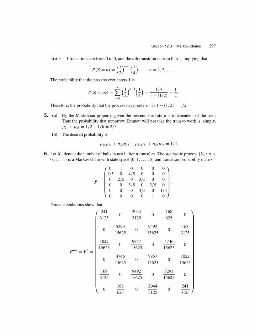
Section 12.3 Markov Chains 297
first n − 1 transitions are from 0 to 0, and the nth transition is from 0 to 1, implying that
P(Z = n) =(1
2
)n−1(1
4
), n = 1, 2, . . . .
The probability that the process ever enters 1 is
P(Z < ∞) =∞∑
n=1
(1
2
)n−1(1
4
)= 1/4
1 − (1/2)= 1
2.
Therefore, the probability that the process never enters 1 is 1 − (1/2) = 1/2.
5. (a) By the Markovian property, given the present, the future is independent of the past.Thus the probability that tomorrow Emmett will not take the train to work is, simply,p21 + p23 = 1/2 + 1/6 = 2/3.
(b) The desired probability is
p21p11 + p21p13 + p23p31 + p23p33 = 1/4.
6. Let Xn denote the number of balls in urn I after n transfers. The stochastic process {Xn : n =0, 1, . . . } is a Markov chain with state space {0, 1, . . . , 5} and transition probability matrix
P =
⎛⎜⎜⎜⎜⎜⎜⎝
0 1 0 0 0 01/5 0 4/5 0 0 00 2/5 0 3/5 0 00 0 3/5 0 2/5 00 0 0 4/5 0 1/50 0 0 0 1 0
⎞⎟⎟⎟⎟⎟⎟⎠ .
Direct calculations show that
P (6) = P 6 =
⎛⎜⎜⎜⎜⎜⎜⎜⎜⎜⎜⎜⎜⎜⎜⎜⎜⎜⎜⎜⎜⎜⎜⎜⎜⎜⎝
241
31250
2044
31250
168
6250
05293
156250
9492
156250
168
3125
1022
156250
9857
156250
4746
156250
04746
156250
9857
156250
1022
15625
168
31250
9492
156250
5293
156250
0168
6250
2044
31250
241
3125
⎞⎟⎟⎟⎟⎟⎟⎟⎟⎟⎟⎟⎟⎟⎟⎟⎟⎟⎟⎟⎟⎟⎟⎟⎟⎟⎠
.

298 Chapter 12 Stochastic Processes
Hence, by Theorem 12.5,
P(X6 = 4) = 0 · 168
625+ 1
15· 0 + 2
15· 4746
15625+ 3
15· 0 + 4
15· 5293
15625+ 5
15· 0 = 0.1308.
7. By drawing a transition graph, it is readily seen that this Markov chain consists of the recurrentclasses {0, 3} and {2, 4} and the transient class {1}.
8. Let Zn be the outcome of the nth toss. Then
Xn+1 = max(Xn, Zn+1)
shows that {Xn : n = 1, 2, . . . } is a Markov chain. Its state space is {1, 2, . . . , 6}, and itstransition probability matrix is given by
P =
⎛⎜⎜⎜⎜⎜⎜⎝
1/6 1/6 1/6 1/6 1/6 1/60 2/6 1/6 1/6 1/6 1/60 0 3/6 1/6 1/6 1/60 0 0 4/6 1/6 1/60 0 0 0 5/6 1/60 0 0 0 0 1
⎞⎟⎟⎟⎟⎟⎟⎠ .
It is readily seen that no two states communicate with each other. Therefore, we have sixclasses of which {1}, {2}, {3}, {4}, {5}, are transient, and {6} is recurrent (in fact, absorbing).
9. This can be achieved more easily by drawing a transition graph. An example of a desiredmatrix is as follows:
⎛⎜⎜⎜⎜⎜⎜⎜⎜⎜⎜⎝
0 0 1/2 0 1/2 0 0 01 0 0 0 0 0 0 00 1 0 0 0 0 0 00 0 1/3 2/3 0 0 0 00 0 0 0 0 2/5 0 3/50 0 0 0 1/2 0 1/2 00 0 0 0 0 3/5 0 2/50 0 0 0 1/3 0 2/3 0
⎞⎟⎟⎟⎟⎟⎟⎟⎟⎟⎟⎠.
10. For 1 ≤ i ≤ 7, starting from state i, let xi be the probability that the Markov chain willeventually be absorbed into state 4. We are interested in x6. Applying the law of total

Section 12.3 Markov Chains 299
probability repeatedly, we obtain the following system of linear equations:⎧⎪⎪⎪⎪⎪⎪⎪⎪⎪⎪⎪⎪⎪⎪⎨⎪⎪⎪⎪⎪⎪⎪⎪⎪⎪⎪⎪⎪⎪⎩
x1 = (0.3)x1 + (0.7)x2
x2 = (0.3)x1 + (0.2)x2 + (0.5)x3
x3 = (0.6)x4 + (0.4)x5
x4 = 1
x5 = x3
x6 = (0.1)x1 + (0.3)x2 + (0.1)x3 + (0.2)x5 + (0.2)x6 + (0.1)x7
x7 = 0.
Solving this system of equations, we obtain⎧⎪⎪⎨⎪⎪⎩x1 = x2 = x3 = x4 = x5 = 1
x6 = 0.875
x7 = 0.
Therefore, the probability is 0.875 that, starting from state 6, the Markov chain will eventuallybe absorbed into state 4.
11. Let π1, π2, and π3 be the long-run probabilities that the sportsman devotes to horseback riding,sailing, and scuba diving, respectively. Then, by Theorem 12.7, π1, π2, and π3 are obtainedfrom solving the system of equations.⎛⎝π1
π2
π3
⎞⎠ =⎛⎝0.20 0.32 0.60
0.30 0.15 0.130.50 0.53 0.27
⎞⎠⎛⎝π1
π2
π3
⎞⎠along with π1 + π2 + π3 = 1. The matrix equation above gives us the following system ofequations ⎧⎪⎨⎪⎩
π1 = 0.20π1 + 0.32π2 + 0.60π3
π2 = 0.30π1 + 0.15π2 + 0.13π3
π3 = 0.50π1 + 0.53π2 + 0.27π3.
By choosing any two of these equations along with π1 + π2 + π3 = 1, we obtain a system ofthree equations in three unknowns. Solving that system yields π1 = 0.38856, π2 = 0.200056,and π3 = 0.411383. Hence the long-run probability that on a randomly selected vacation daythe sportsman sails is approximately 0.20.
12. For n ≥ 1, let
Xn ={
1 if the nth fish caught is trout
0 if the nth fish caught is not trout.
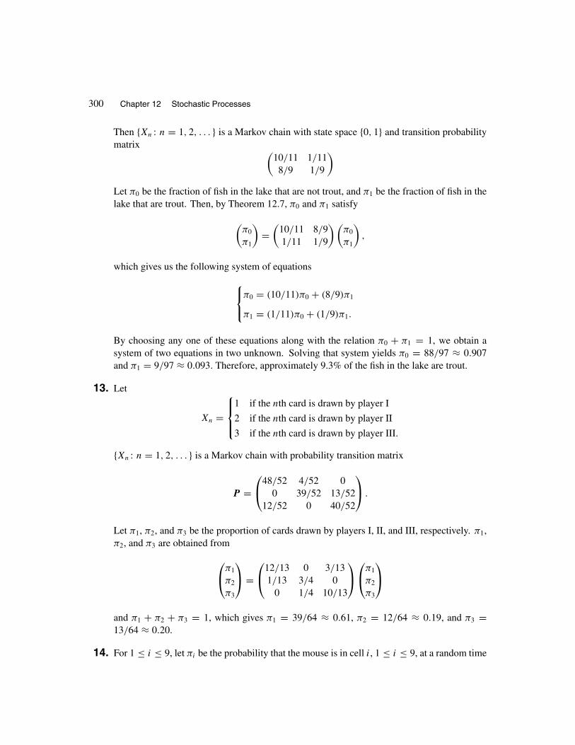
300 Chapter 12 Stochastic Processes
Then {Xn : n = 1, 2, . . . } is a Markov chain with state space {0, 1} and transition probabilitymatrix (
10/11 1/118/9 1/9
)Let π0 be the fraction of fish in the lake that are not trout, and π1 be the fraction of fish in thelake that are trout. Then, by Theorem 12.7, π0 and π1 satisfy(
π0
π1
)=(
10/11 8/91/11 1/9
)(π0
π1
),
which gives us the following system of equations⎧⎨⎩π0 = (10/11)π0 + (8/9)π1
π1 = (1/11)π0 + (1/9)π1.
By choosing any one of these equations along with the relation π0 + π1 = 1, we obtain asystem of two equations in two unknown. Solving that system yields π0 = 88/97 ≈ 0.907and π1 = 9/97 ≈ 0.093. Therefore, approximately 9.3% of the fish in the lake are trout.
13. Let
Xn =
⎧⎪⎨⎪⎩1 if the nth card is drawn by player I
2 if the nth card is drawn by player II
3 if the nth card is drawn by player III.
{Xn : n = 1, 2, . . . } is a Markov chain with probability transition matrix
P =⎛⎝48/52 4/52 0
0 39/52 13/5212/52 0 40/52
⎞⎠ .
Let π1, π2, and π3 be the proportion of cards drawn by players I, II, and III, respectively. π1,π2, and π3 are obtained from⎛⎝π1
π2
π3
⎞⎠ =⎛⎝12/13 0 3/13
1/13 3/4 00 1/4 10/13
⎞⎠⎛⎝π1
π2
π3
⎞⎠and π1 + π2 + π3 = 1, which gives π1 = 39/64 ≈ 0.61, π2 = 12/64 ≈ 0.19, and π3 =13/64 ≈ 0.20.
14. For 1 ≤ i ≤ 9, let πi be the probability that the mouse is in cell i, 1 ≤ i ≤ 9, at a random time

Section 12.3 Markov Chains 301
in the future. Then πi’s satisfy⎛⎜⎜⎜⎜⎜⎜⎜⎜⎜⎜⎜⎜⎝
π1
π2
π3
π4
π5
π6
π7
π8
π9
⎞⎟⎟⎟⎟⎟⎟⎟⎟⎟⎟⎟⎟⎠=
⎛⎜⎜⎜⎜⎜⎜⎜⎜⎜⎜⎜⎜⎝
0 1/3 0 1/3 0 0 0 0 01/2 0 1/2 0 1/4 0 0 0 00 1/3 0 0 0 1/3 0 0 0
1/2 0 0 0 1/4 0 1/2 0 00 1/3 0 1/3 0 1/3 0 1/3 00 0 1/2 0 1/4 0 0 0 1/20 0 0 1/3 0 0 0 1/3 00 0 0 0 1/4 0 1/2 0 1/20 0 0 0 0 1/3 0 1/3 0
⎞⎟⎟⎟⎟⎟⎟⎟⎟⎟⎟⎟⎟⎠
⎛⎜⎜⎜⎜⎜⎜⎜⎜⎜⎜⎜⎜⎝
π1
π2
π3
π4
π5
π6
π7
π8
π9
⎞⎟⎟⎟⎟⎟⎟⎟⎟⎟⎟⎟⎟⎠.
Solving this system of equations along with∑9
i=1 π1, we obtain
π1 = π3 = π7 = π9 = 1/12,
π2 = π4 = π6 = π8 = 1/8,
π5 = 1/6.
15. Let Xn denote the number of balls in urn I after n transfers. The stochastic process {Xn : n =0, 1, . . . } is a Markov chain with state space {0, 1, . . . , 5} and transition probability matrix
P =
⎛⎜⎜⎜⎜⎜⎜⎝
0 1 0 0 0 01/5 0 4/5 0 0 00 2/5 0 3/5 0 00 0 3/5 0 2/5 00 0 0 4/5 0 1/50 0 0 0 1 0
⎞⎟⎟⎟⎟⎟⎟⎠ .
Clearly, {Xn : n = 0, 1, . . . } is an irreducible recurrent Markov chain; since it is finite-state,it is positive recurrent. However, {Xn : n = 0, 1, . . . } is not aperiodic, and the period of eachstate is 2. Hence the limiting probabilities do not exist. For 0 ≤ i ≤ 5, let πi be the fraction oftime urn I contains i balls. Then with this interpretation, πi’s satisfy the following equations⎛⎜⎜⎜⎜⎜⎜⎝
π0
π1
π2
π3
π4
π5
⎞⎟⎟⎟⎟⎟⎟⎠ =
⎛⎜⎜⎜⎜⎜⎜⎝
0 1/5 0 0 0 01 0 2/5 0 0 00 4/5 0 3/5 0 00 0 3/5 0 4/5 00 0 0 2/5 0 10 0 0 0 1/5 0
⎞⎟⎟⎟⎟⎟⎟⎠
⎛⎜⎜⎜⎜⎜⎜⎝
π0
π1
π2
π3
π4
π5
⎞⎟⎟⎟⎟⎟⎟⎠ ,
∑5i=0 πi = 1. Solving these equations, we obtain
π0 = π5 = 1/31,
π1 = π4 = 5/31,
π2 = π3 = 10/31.

302 Chapter 12 Stochastic Processes
Therefore, the fraction of time an urn is empty is π0 +π5 = 2/31. Hence the expected numberof balls transferred between two consecutive times that an urn becomes empty is 31/2 = 15.5.
16. Solution 1: Let Xn be the number of balls in urn I immediately before the nth game begins.Then {Xn : n = 1, 2, . . . } is a Markov chain with state space {0, 1, . . . , 7} and transitionprobability matrix
P =
⎛⎜⎜⎜⎜⎜⎜⎜⎜⎜⎜⎝
3/4 1/4 0 0 0 0 0 01/4 1/2 1/4 0 0 0 0 00 1/4 1/2 1/4 0 0 0 00 0 1/4 1/2 1/4 0 0 00 0 0 1/4 1/2 1/4 0 00 0 0 0 1/4 1/2 1/4 00 0 0 0 0 1/4 1/2 1/40 0 0 0 0 0 1/4 3/4
⎞⎟⎟⎟⎟⎟⎟⎟⎟⎟⎟⎠.
Since the transition probability matrix is doubly stochastic; that is, the sum of each columnis also 1, for i = 0, 1, . . . , 7, πi , the long-run probability that the number of balls in urn Iimmediately before a game begins is 1/8 (see Example 12.35). This implies that the long-runprobability mass function of the number of balls in urn I or II is 1/8 for i = 0, 1, . . . , 7.
Solution 2: Let Xn be the number of balls in the urn selected at step 1 of the nth game. Then{Xn : n = 1, 2, . . . } is a Markov chain with state space {0, 1, . . . , 7} and transition probabilitymatrix
P =
⎛⎜⎜⎜⎜⎜⎜⎜⎜⎜⎜⎝
1/2 0 0 0 0 0 0 1/21/4 1/4 0 0 0 0 1/4 1/40 1/4 1/4 0 0 1/4 1/4 00 0 1/4 1/4 1/4 1/4 0 00 0 0 1/2 1/2 0 0 00 0 1/4 1/4 1/4 1/4 0 00 1/4 1/4 0 0 1/4 1/4 0
1/4 1/4 0 0 0 0 1/4 1/4
⎞⎟⎟⎟⎟⎟⎟⎟⎟⎟⎟⎠.
Since the transition probability matrix is doubly stochastic; that is, the sum of each columnis also 1, for i = 0, 1, . . . , 7, πi , the long-run probability that the number of balls in theurn selected at step 1 of a game is 1/8 (see Example 12.35). This implies that the long-runprobability mass function of the number of balls in urn I or II is 1/8 for i = 0, 1, . . . , 7.
17. For i ≥ 0, state i is directly accessible from 0. On the other hand, i is accessible from i + 1.These two facts make it possible for all states to communicate with each other. Therefore, theMarkov chain has only one class. Since 0 is recurrent and aperiodic (note that p00 > 0 makes0 aperiodic), all states are recurrent and aperiodic. Let πk be the long-run probability that a

Section 12.3 Markov Chains 303
computer selected at the end of a semester will last at least k additional semesters. Solving⎛⎜⎜⎜⎝π0
π1
π2...
⎞⎟⎟⎟⎠ =
⎛⎜⎜⎜⎝p1 1 0 0 . . .
p2 0 1 0 . . .
p3 0 0 1 . . ....
⎞⎟⎟⎟⎠⎛⎜⎜⎜⎝
π0
π1
π2...
⎞⎟⎟⎟⎠along with
∑∞i=0 πi = 1, we obtain
π0 = 1
1 +∑∞i=1(1 − p1 − p2 − · · · − pi)
,
πk = 1 − p1 − p2 − · · · − pk
1 +∑∞i=1(1 − p1 − p2 − · · · − pi)
, k ≥ 1.
18. Let DN denote the state at which the last movie Mr. Gorfin watched was not a drama, butthe one before that was a drama. Define DD, ND, and NN similarly, and label the statesDD, DN , ND, and NN by 0, 1, 2, and 3, respectively. Let Xn = 0 if the nth and (n − 1)stmovies Mr. Gorfin watched were both dramas. Define Xn = 1, 2, and 3 similarly. Then{Xn : n = 1, 2, . . . } is a Markov chain with state space {0, 1, 2, 3} and transition probabilitymatrix
P =
⎛⎜⎜⎝7/8 1/8 0 00 0 1/2 1/2
1/2 1/2 0 00 0 1/8 7/8
⎞⎟⎟⎠ .
(a) If the first two movies Mr. Gorfin watched last weekend were dramas, the probabilitythat the fourth one is a drama is p2
00 + p202. Since
P 2 =
⎛⎜⎜⎝49/64 7/64 1/16 1/161/4 1/4 1/16 7/167/16 1/16 1/4 1/41/16 1/16 7/64 49/64
⎞⎟⎟⎠ ,
the desired probability is (49/64) + (1/16) = 53/64.
(b) Let π0 denote the long-run probability that Mr. Gorfin watches two dramas in a row.Define π1, π2, and π3 similarly. We have that,⎛⎜⎜⎝
π0
π1
π2
π3
⎞⎟⎟⎠ =
⎛⎜⎜⎝7/8 0 1/2 01/8 0 1/2 00 1/2 0 1/80 1/2 0 7/8
⎞⎟⎟⎠⎛⎜⎜⎝
π0
π1
π2
π3
⎞⎟⎟⎠ .
Solving this system along with π0 +π1 +π2 +π3 = 1, we obtain π0 = 2/5, π1 = 1/10,π2 = 1/10, and π3 = 2/5. Hence the probability that Mr. Gorfin watches two dramasin a row is 2/5.

304 Chapter 12 Stochastic Processes
19. Clearly,
Xn+1 ={
0 if the (n + 1)st outcome is 6
1 + Xn otherwise.
This relation shows that {Xn : n = 1, 2, . . . } is a Markov chain. Its transition probabilitymatrix is given by
P =
⎛⎜⎜⎜⎜⎜⎝1/6 5/6 0 0 0 . . .
1/6 0 5/6 0 0 . . .
1/6 0 0 5/6 0 . . .
1/6 0 0 0 5/6 . . ....
⎞⎟⎟⎟⎟⎟⎠ .
It is readily seen that all states communicate with 0. Therefore, by transitivity of the com-munication property, all states communicate with each other. Therefore, the Markov chain isirreducible. Clearly, 0 is recurrent. Since p00 > 0, it is aperiodic as well. Hence all statesare recurrent and aperiodic. On the other hand, starting at 0, the expected number of transi-tions until the process returns to 0 is 6. This is because the number of tosses until the next6 obtained is a geometric random variable with probability of success p = 1/6, and henceexpected value 1/p = 6. Therefore, 0, and hence all other states are positive recurrent. Next,a simple probabilistic argument shows that,
πi =(5
6
)i(1
6
), i = 0, 1, 2, . . . .
This can also be shown by solving the following system of equations:⎧⎪⎪⎪⎪⎪⎪⎪⎪⎪⎨⎪⎪⎪⎪⎪⎪⎪⎪⎪⎩
⎛⎜⎜⎜⎜⎜⎜⎜⎝
π0
π1
π2
π3...
⎞⎟⎟⎟⎟⎟⎟⎟⎠=
⎛⎜⎜⎜⎜⎜⎜⎜⎝
1/6 1/6 1/6 1/6 . . .
5/6 0 0 0 . . .
0 5/6 0 0 . . .
0 0 5/6 0 . . ....
⎞⎟⎟⎟⎟⎟⎟⎟⎠
⎛⎜⎜⎜⎜⎜⎜⎜⎝
π0
π1
π2
π3...
⎞⎟⎟⎟⎟⎟⎟⎟⎠π0 + π1 + π2 + · · · = 1.
20. (a) Let
Xn ={
1 if Alberto wins the nth game
0 if Alberto loses the nth game.
Then {Xn : n = 1, 2, . . . } is a Markov chain with state space {0, 1}. Its transition
probability matrix is P =(
1 − p pp 1 − p
). Using induction, we will now show that
P (n) = P n =
⎛⎜⎜⎝1
2+ 1
2(1 − 2p)n 1
2− 1
2(1 − 2p)n
1
2− 1
2(1 − 2p)n 1
2+ 1
2(1 − 2p)n
⎞⎟⎟⎠ .

Section 12.3 Markov Chains 305
Clearly, for n = 1, P (1) = P . Suppose that
P (n) =
⎛⎜⎜⎜⎝1
2+ 1
2(1 − 2p)n 1
2− 1
2(1 − 2p)n
1
2− 1
2(1 − 2p)n 1
2+ 1
2(1 − 2p)n
⎞⎟⎟⎟⎠ .
We will show that
P n+1 =
⎛⎜⎜⎜⎝1
2+ 1
2(1 − 2p)n+1 1
2− 1
2(1 − 2p)n+1
1
2− 1
2(1 − 2p)n+1 1
2+ 1
2(1 − 2p)n+1
⎞⎟⎟⎟⎠ .
To do so, note that
P (n+1) =(
p00 p01
p10 p11
)(pn
00 pn01
pn10 pn
11
)=(
p00pn00 + p01p
n10 p00p
n01 + p01p
n11
p10pn00 + p11p
n10 p10p
n01 + p11p
n11
).
Thus
pn+111 = p10p
n01 + p11p
n11 = p
[1
2− 1
2(1 − 2p)n
]+ (1 − p)
[1
2+ 1
2(1 − 2p)n
]= 1
2
[p + (1 − p)
]+ 1
2(1 − 2p)n
[− p + (1 − p)] = 1
2+ 1
2(1 − 2p)n+1.
This establishes what we wanted to show. The proof that pn+100 = 1
2+ 1
2(1 − 2p)n+1 is
identical to what we just showed. We have
P n+101 = 1 − P n+1
00 = 1 −[1
2+ 1
2(1 − 2p)n
]= 1
2− 1
2(1 − 2p)n.
Similarly,
pn+110 = 1 − pn+1
11 = 1
2− 1
2(1 − 2p)n.
(b) Let π0 and π1 be the long-run probabilities that Alberto loses and wins a game, respec-tively. Then (
π0
π1
)=(
1 − p p
p 1 − p
)(π0
π1
),
and π0 + π1 = 1 imply that π0 = π1 = 1/2. Therefore, the expected number of gamesAlberto will play between two consecutive wins is 1/π1 = 2.

306 Chapter 12 Stochastic Processes
21. For each j ≥ 0, limn→∞ pnij exists and is independent of i if the following system of equations,
in π0, π1, . . . , have a unique solution.⎧⎪⎪⎪⎪⎪⎪⎪⎪⎪⎨⎪⎪⎪⎪⎪⎪⎪⎪⎪⎩
⎛⎜⎜⎜⎜⎜⎜⎜⎝
π0
π1
π2
π3...
⎞⎟⎟⎟⎟⎟⎟⎟⎠=
⎛⎜⎜⎜⎜⎜⎜⎜⎝
1 − p 1 − p 0 0 0 0 . . .
p 0 1 − p 0 0 0 . . .
0 p 0 1 − p 0 0 . . .
0 0 p 0 1 − p 0 . . ....
⎞⎟⎟⎟⎟⎟⎟⎟⎠
⎛⎜⎜⎜⎜⎜⎜⎜⎝
π0
π1
π2
π3...
⎞⎟⎟⎟⎟⎟⎟⎟⎠π0 + π1 + π2 + · · · = 1.
From the matrix equation, we obtain
πi =( p
1 − p
)i
π0, i = 0, 1, . . . .
For these quantities to satisfy∑∞
i=0 πi = 1, we need the geometric series∞∑i=0
( p
1 − p
)i
to
converge. Hence we must have p < 1 − p, or p < 1/2. Therefore, for p < 1/2, thisirreducible, aperiodic Markov chain which is positively recurrent has limiting probabilities.Note that, for p < 1/2,
π0
∞∑i=0
( p
1 − p
)i = 1
yields π0 = 1 − p
1 − p. Thus the limiting probabilities are
πi =( p
1 − p
)i(1 − p
1 − p
), i = 0, 1, 2, . . . .
22. Let Yn be Carl’s fortune after the nth game. Let Xn be Stan’s fortune after the nth game. LetZn = Yn − Xn. The {Zn : n = 0, 1, . . . } is a random walk with state space {0, ±2, ±4, . . . }.We have that Z0 = 0, and at each step either the process moves two units to the right withprobability 0.46 or two units to the left with probability 0.54. Let A be the event that, startingat 0, the random walk will eventually enter 2; P(A) is the desired quantity. By the law of totalprobability,
P(A) = P(A | Z1 = 2)P (Z1 = 2) + P(A | Z1 = −2)P (Z1 = −2)
= 1 · (0.46) + [P(A)
]2 · (0.54).
To show that P(A | Z1 = −2) = [P(A)
]2, let E be the event of, starting from −2, eventually
entering 0. It should be clear that P(E) = P(A). By independence of E and A, we have
P(A | Z = −2) = P(EA) = P(E)P (A) = [P(A)
]2.

Section 12.3 Markov Chains 307
We have shown that P(A), the quantity we are interested in, satisfies
(0.54)[P(A)
]2 − P(A) + 0.46 = 0.
This is a quadratic equation in P(A). Solving it gives P(A) = 23/27 ≈ 0.85.
23. We will use induction on m. For m = 1, the relation is, simply, the Markovian property, whichis true. Suppose that the relation is valid for m − 1. We will show that it is also valid for m.We have
P(Xn+m = j | X0 = i0, X1 = i1, . . . , Xn = in)
=∑i∈S
P(Xn+m = j | X0 = i0, . . . , Xn = in, Xn+m−1 = i)
P (Xn+m−1 = i | X0 = i0, . . . , Xn = in)
=∑i∈S
P(Xn+m = j | Xn+m−1 = i)P (Xn+m−1 = i | Xn = in)
=∑i∈S
P (Xn+m = j | Xn+m−1 = i, Xn = in)P (Xn+m−1 = i | Xn = in)
= P(Xn+m = j | Xn = in),
where the following relations are valid from the definition of Markov chain: given the presentstate, the process is independent of the past.
P(Xn+m = j | X0 = i0, . . . , Xn = in, Xn+m−1 = i) = P(Xn+m = j | Xn+m−1 = i),
P (Xn+m = j | Xn+m−1 = i) = P(Xn+m = j | Xn+m−1 = i, Xn = in).
24. Let (0, 0), the origin, be denoted by O. It should be clear that, for all n ≥ 0, P 2n+1OO = 0. Now,
for n ≥ 1, let Z1, Z2, Z3, and Z4 be the number of transitions to the right, left, up, and down,respectively. The joint probability mass function of Z1, Z2, Z3, and Z4 is multinomial. Wehave
P 2nOO =
n∑i=0
P(Z1 = i, Z2 = i, Z3 = n − i, Z4 = n − i)
=n∑
i=0
(2n)!i! i! (n − i)! (n − i)!
(1
4
)i(1
4
)i(1
4
)n−i(1
4
)n−i
=n∑
i=0
(2n)!n! n! · n!
i! (n − i)! · n!i! (n − i)!
(1
4
)2n
=(1
4
)2n(
2n
n
) n∑i=0
(n
i
)2
.

308 Chapter 12 Stochastic Processes
By Example 2.28,n∑
i=0
(n
i
)2
=(
2n
n
). Thus P n
OO =(1
4
)2n(
2n
n
)2
. Now, by Theorem 2.7
(Stirling’s formula),(1
4
)2n(
2n
n
)2
=(1
4
)2n ·[(2n)!
n! n!]2 ∼ 1
42n·[ √
4πn (2n)2n e−2n
(√
2πn · nn · e−n)2
]2 = 1
πn.
Therefore,∞∑
n=1
P nOO =
∞∑n=1
(1
4
)2n(
2n
n
)2
is convergent if and only if∞∑
n=1
1
πnis convergent.
Since1
π
∞∑n=1
1
nis divergent,
∑∞n=1 P n
OO is divergent, showing that the state (0, 0) is recurrent.
25. Clearly, P(Xn+1 = 1 | Xn = 0) = 1. For i ≥ 1, given Xn = i, either Xn+1 = i + 1 in whichcase we say that a transition to the right has occurred, or Xn+1 = i − 1 in which case we saythat a transition to the left has occurred. For i ≥ 1, given Xn = i, when the nth transitionoccurs, let S be the remaining service time of the customer being served or the service timeof a new customer, whichever applies. Let T be the time from the nth transition until the nextarrival. By the memoryless property of exponential random variables, S and T are exponentialrandom variables with parameters µ and λ, respectively. For i ≥ 1,
P(Xn+1 = i + 1 | Xn = i) = P(T < S) =∫ ∞
0P(S > T | T = t)λe−λt dt
=∫ ∞
0P(S > t)λe−λt dt =
∫ ∞
0e−µt · λe−λt dt = λ
λ + µ.
Therefore,
P(Xn+1 = i − 1 | Xn = i) = P(T > S) = 1 − λ
λ + µ= µ
λ + µ.
These calculations show that knowing Xn, the next transition does not depend on the values ofXj for j < n. Therefore, {Xn : n = 1, 2, . . . } is a Markov chain, and its transition probabilitymatrix is given by
P =
⎛⎜⎜⎜⎜⎜⎜⎜⎜⎜⎜⎝
0 1 0 0 0 . . .µ
λ + µ0
λ
λ + µ0 0 . . .
0µ
λ + µ0
λ
λ + µ0 . . .
0 0µ
λ + µ0
λ
λ + µ. . .
...
⎞⎟⎟⎟⎟⎟⎟⎟⎟⎟⎟⎠.
Since all states are accessible from each other, this Markov chain is irreducible. Starting from0, for the Markov chain to return to 0, it needs to make as many transitions to the left as it

Section 12.3 Markov Chains 309
makes to the right. Therefore, P n00 > 0 only for positive even integers. Since the greatest
common divisor of such integers is 2, the period of 0, and hence the period of all other statesis 2.
26. The ij th element of PQ is the product of the ith row of P with the jth column of Q. Thus
it is∑
�
pi�q�j . To show that the sum of each row of PQ is 1, we will now calculate the sum
of the elements of the ith row of PQ, which is∑j
∑�
pi�q�j =∑
�
∑j
pi�q�j =∑
�
(pi�
∑j
q�j
)=∑
�
pi� = 1.
Note that∑
j
q�j = 1 and∑
�
pi� = 1 since the sum of the elements of the �th row of Q and
the sum of the elements of the ith row of P are 1.
27. If state j is accessible from state i, there is a path
i = i1, i2, i3, . . . , in = j
from i to j . If n ≤ K , we are done. If n > K , by the pigeonhole principle, there must exist k
and � (k < �) so that ik = i�. Now the path
i = i1, i2, . . . , ik, ik+1, . . . , i�, i�+1, . . . , in = j
can be reduced toi = i1, i2, . . . , ik, i�+1, . . . , in = j
which is still a path from i to j but in fewer steps. Repeating this procedure, we can eliminateall of the states that appear more than once from the path and yet reach from i to j with apositive probability. After all such eliminations are made, we obtain a path
i = i1, im1, im2, . . . , in = j
in which the states i1, im1 , im2 , . . . , in are distinct states. Since there are K states altogether,this path has at most K states.
28. Let I = {n ≥ 1 : pnii > 0} and J = {n ≥ 1 : pn
jj > 0}. Then d(i), the period of i, is thegreatest common divisor of the elements of I , and d(j), the period of j , is the greatest commondivisor of the elements of J . If d(i) �= d(j), then one of d(i) and d(j) is smaller than theother one. We will prove the theorem for the case in which d(j) < d(i). The proof for thecase in which d(i) < d(j) follows by symmetry. Suppose that for positive integers n and m,pn
ij > 0 and pmji > 0. Let k ∈ J ; then pk
jj > 0. We have
pn+mii ≥ pn
ijpmji > 0,

310 Chapter 12 Stochastic Processes
and
pn+k+mii ≥ pn
ijpkjjp
mji > 0.
By these inequalities, we have that d(i) divides n + m and n + k + m. Hence it divides(n + k + m) − (n + m) = k. We have shown that, if k ∈ J , then d(i) divides k. This meansthat d(i) divides all members of J . It contradicts the facts that d(j) is the greatest commondivisor of J and d(j) < d(i). Therefore, we must have d(i) = d(j).
29. The stochastic process {Xn : n = 1, 2, . . . } is a Markov chain with state space {0, 1, . . . , k−1}.For 0 ≤ i ≤ k − 2, a transition is only possible from state i to 0 or i + 1. The only transitionfrom k − 1 is to 0. Let Z be the number of weeks it takes Liz to play again with Bob from thetime they last played. The event Z > i occurs if and only if Liz has not played with Bob sincei Sundays ago, and the earliest she will play with him is next Sunday. Now the probability isi/k that Liz will play with Bob if last time they played was i Sundays ago; hence
P(Z > i) = 1 − i
k, i = 1, 2, . . . , k − 1.
Using this fact, for 0 ≤ i ≤ k − 2, we obtain
pi(i+1) = P(Xn+1 = i + 1 | Xn = i) = P(Xn = i, Xn+1 = i + 1)
P (Xn = i)
= P(Z > i + 1)
P (Z > i)=
1 − i + 1
k
1 − i
k
= k − i − 1
k − i,
pi0 = P(Xn+1 = 0 | Xn = i) = 1 − k − i − 1
k − i= 1
k − i,
p(k−1)0 = P(Xn+1 = 0 | Xn = k − 1) = 1.
Hence the transition probability matrix of {Xn : n = 1, 2, . . . } is given by

Section 12.3 Markov Chains 311
P =
⎛⎜⎜⎜⎜⎜⎜⎜⎜⎜⎜⎜⎜⎜⎜⎜⎜⎜⎜⎜⎜⎜⎜⎜⎜⎜⎜⎜⎜⎝
1
k1 − 1
k0 0 0 . . . 0 0
1
k − 10 1 − 1
k − 10 0 . . . 0 0
1
k − 20 0 1 − 1
k − 20 . . . 0 0
1
k − 30 0 0 1 − 1
k − 3. . . 0 0
...
1
20 0 0 0 . . . 0
1
2
1 0 0 0 0 . . . 0 0
⎞⎟⎟⎟⎟⎟⎟⎟⎟⎟⎟⎟⎟⎟⎟⎟⎟⎟⎟⎟⎟⎟⎟⎟⎟⎟⎟⎟⎟⎠
.
It should be clear that the Markov chain under consideration is irreducible, aperiodic, andpositively recurrent. For 0 ≤ i ≤ k − 1, let πi be the long-run probability that Liz says no toBob for i consecutive weeks. π0, π1, . . . , πk−1 are obtained from solving the following matrixequation along with
∑k−1i=0 πi = 1.
⎛⎜⎜⎜⎜⎜⎜⎜⎜⎜⎜⎜⎜⎜⎜⎜⎜⎜⎜⎜⎜⎜⎝
π0
π1
π2
π3
...
πk−2
πk−1
⎞⎟⎟⎟⎟⎟⎟⎟⎟⎟⎟⎟⎟⎟⎟⎟⎟⎟⎟⎟⎟⎟⎠
=
⎛⎜⎜⎜⎜⎜⎜⎜⎜⎜⎜⎜⎜⎜⎜⎜⎜⎜⎜⎜⎜⎜⎜⎜⎜⎜⎜⎜⎜⎜⎜⎝
1
k
1
k − 1
1
k − 2
1
k − 3. . . 1
2 1
1 − 1
k0 0 0 . . . 0 0
0 1 − 1
k − 10 0 . . . 0 0
0 0 1 − 1
k − 20 . . . 0 0
0 0 0 1 − 1
k − 3. . . 0 0
...
0 0 0 0 . . .1
20
⎞⎟⎟⎟⎟⎟⎟⎟⎟⎟⎟⎟⎟⎟⎟⎟⎟⎟⎟⎟⎟⎟⎟⎟⎟⎟⎟⎟⎟⎟⎟⎠
⎛⎜⎜⎜⎜⎜⎜⎜⎜⎜⎜⎜⎜⎜⎜⎜⎜⎜⎜⎜⎜⎜⎝
π0
π1
π2
π3
...
πk−2
πk−1
⎞⎟⎟⎟⎟⎟⎟⎟⎟⎟⎟⎟⎟⎟⎟⎟⎟⎟⎟⎟⎟⎟⎠
.
The matrix equation gives
πi = k − i
kπ0, i = 1, 2, . . . , k − 1.

312 Chapter 12 Stochastic Processes
Using∑k−1
i=0 πi = 1, we obtain
π0
k−1∑i=0
k − i
k= 1
or, equivalently,
π0
k
[ k−1∑i=0
k −k−1∑i=0
i]
= 1.
This implies thatπ0
k
[k2 − (k − 1)k
2
]= 1,
which gives π0 = 2/(k + 1). Hence
πi = 2(k − i)
k(k + 1), i = 0, 1, 2, . . . , k − 1.
30. Let Xi be the amount of money player A has after i games. Clearly, X0 = a and {Xn : n =0, 1, . . . } is a Markov chain with state space {0, 1, . . . , a, a + 1, . . . , a + b}. For 0 ≤ i ≤a + b, let mi = E(T | X0 = i). Let F be the event that A wins the first game. Then, for1 ≤ i ≤ a + b − 1,
E(T | X0 = i) = E(T | X0 = i, F )P (F | X0 = i) + E(T | X0 = i, F c)P (F c | X0 = i).
This gives
mi = (1 + mi+1)1
2+ (1 + mi−1)
1
2, 1 ≤ i ≤ a + b − 1,
or, equivalently,2mi = 2 + mi+1 + mi−1, 1 ≤ i ≤ a + b − 1.
Now rewrite this relation as
mi+1 − mi = −2 + mi − mi−1, 1 ≤ i ≤ a + b − 1,
and, for 1 ≤ i ≤ a + b, letyi = mi − mi−1.
Thenyi+1 = −2 + yi, 1 ≤ i ≤ a + b − 1,
and, for 1 ≤ i ≤ a + b,mi = y1 + y2 + · · · + yi.
Clearly, m0 = 0, ma+b = 0, y1 = m1, and
y2 = −2 + y1 = −2 + m1,
y3 = −2 + y2 = −2 + (−2 + m1) = −4 + m1
...
yi = −2(i − 1) + m1, 1 ≤ i ≤ a + b.

Section 12.3 Markov Chains 313
Hence, for 1 ≤ i ≤ a + b,
mi = y1 + y2 + · · · + yi
= im1 − 2[1 + 2 + · · · + (i − 1)
]= im1 − i(i − 1) = i(m1 − i + 1).
This and ma+b = 0 imply that
(a + b)(m1 − a − b + 1) = 0,
or m1 = a + b − 1. Therefore,mi = i(a + b − i),
and hence the desired quantity is
E(T | X0 = a) = ma = ab.
31. Let q be a positive solution of the equation x = ∑∞i=0 αix
i . Then q = ∑∞i=0 αiq
i . We willshow that ∀n ≥ 0, P(Xn = 0) ≤ q. This implies that
p = limn→∞ P(Xn = 0) ≤ q.
To establish that P(Xn = 0) ≤ q, we use induction. For n = 0, P(X0 = 0) = 0 ≤ q istrivially true. Suppose that P(Xn = 0) ≤ q. We have
P(Xn+1 = 0) =∞∑i=0
P(Xn+1 = 0 | X1 = i)P (X1 = i).
It should be clear that
P(Xn+1 = 0 | X1 = i) = [P(Xn = 0 | X0 = 1)
]i.
However, since P(X0 = 1) = 1,
P(Xn = 0 | X0 = 1) = P(Xn = 0).
Therefore,P(Xn+1 = 0 | X1 = i) = [
P(Xn = 0)]i
.
Thus
P(Xn+1 = 0) =∞∑i=0
[P(Xn = 0)
]iP (X1 = i) ≤
∞∑i=0
qiαi = q.
This establishes the theorem.

314 Chapter 12 Stochastic Processes
32. Multiplying P successively, we obtain
p12 = 1
13
p212 =
( 9
13
)( 1
13
)+ 1
13,
p312 =
( 9
13
)2( 1
13
)+( 9
13
)( 1
13
)+ 1
13,
and in general,
pn12 = 1
13
[( 9
13
)n−1 +( 9
13
)n−2 + · · · + 1]
= 1
13·
1 −( 9
13
)n
1 − 9
13
= 1
4
[1 −
( 9
13
)n].
Hence the desired probability is limn→∞ pn12 = 1/4.
33. We will use induction. Let n = 1; then, for 1 + j − i to be nonnegative, we must have
i − 1 ≤ j . For the inequality1 + j − i
2≤ 1 to be valid, we must have j ≤ i + 1. Therefore,
i − 1 ≤ j ≤ i + 1. But, for j = i, 1 + j − i is not even. Therefore, if 1 + j − i is an even
nonnegative integer satisfying1 + j − i
2≤ 1, we must have j = i − 1 or j = i + 1. For
j = i − 1,
n + j − i
2= 1 + i − 1 − i
2= 0 and
n − j + i
2= 1 − i + 1 + i
2= 1.
Hence
P(X1 = i − 1 | X0 = i) = 1 − p =(
1
0
)p0(1 − p)1,
showing that the relation is valid. For j = i + 1,
n + j − i
2= 1 + i + 1 − i
2= 1 and
n − j + i
2= 1 − i − 1 + i
2= 0.
Hence
P(X1 = i + 1 | X0 = i) = p =(
1
1
)p1(1 − p)0,
showing that the relation is valid in this case as well. Since, for a simple random walk, theonly possible transitions from i are to states i + 1 and i − 1, in all other cases
P(X1 = j | X0 = i) = 0.

Section 12.4 Continuous-Time Markov Chains 315
We have established the theorem for n = 1. Now suppose that it is true for n. We will showit for n + 1 by conditioning on Xn:
P(Xn+1 = j | X0 = i) = P(Xn+1 = j | X0 = i, Xn = j − 1)P (Xn = j − 1 | X0 = i)
+ P(Xn+1 = j | X0 = i, Xn = j + 1)P (Xn = j + 1 | X0 = i)
= P(Xn+1 = j | Xn = j − 1)P (Xn = j − 1 | X0 = i)
+ P(Xn+1 = j | Xn = j + 1)P (Xn = j + 1 | X0 = i)
= p ·(
nn + j − 1 − i
2
)p(n+j−1−i)/2(1 − p)(n−j+1+i)/2
+ (1 − p)
(n
n + j + 1 − i
2
)p(n+j+1−i)/2(1 − p)(n−j−1+i)/2
=[(
nn − 1 + j − i
2
)+(
nn + 1 + j − i
2
)]p(n+1+j−i)/2(1 − p)(n+1−j+i)/2
=(
n + 1n + 1 + j − i
2
)p(n+1+j−i)/2(1 − p)(n+1−j+i)/2.
12.4 CONTINUOUS-TIME MARKOV CHAINS
1. By Chapman-Kolmogorov equations,
pij (t + h) − pij (t) =∞∑
k=0
pik(h)pkj (t) − pij (t)
=∑k �=i
pik(h)pkj (t) + pii(h)pij (t) − pij (t)
=∑k �=i
pik(h)pkj (t) + pij (t)[pii(h) − 1
].
Thuspij (t + h) − pij (t)
h=∑k �=i
pik(h)
hpkj (t) − pij (t)
1 − pii(h)
h.
Letting h → 0, by (12.13) and (12.14), we have
p′ij (t) =
∑k �=i
qikpkj (t) − νipij (t).

316 Chapter 12 Stochastic Processes
2. Clearly,{X(t) : t ≥ }
is a continuous-time Markov chain. Its balance equations are as follows:
State Input rate to = Output rate from
f µπ0 = λπf
0 λπf + µπ1 + µπ2 + µπ3 = µπ0 + λπ0
1 λπ0 = λπ1 + µπ1
2 λπ1 = λπ2 + µπ2
3 λπ2 = µπ3.
Solving these equations along with
πf + π0 + π1 + π2 + π3 = 1
we obtain
πf = µ2
λ(λ + µ), π0 = µ
λ + µ,
π1 = λµ
(λ + µ)2, π2 = λ2µ
(λ + µ)3,
π3 =( λ
λ + µ
)3.
3. The fact that{X(t) : t ≥ 0
}is a continuous-time Markov chain should be clear. The balance
equations are
State Input rate to = Output rate from
(0, 0) µπ(1,0) + λπ(0,1) = λπ(0,0) + µπ(0,0)
(n, 0) µπ(n+1,0) + λπ(n−1,0) = λπ(n,0) + µπ(n,0), n ≥ 1
(0, m) λπ(0,m+1) + µπ(0,m−1) = λπ(0,m) + µπ(0,m) m ≥ 1.
4. Let X(t) be the number of customers in the system at time t . Then the process{X(t) : t ≥ 0
}is a birth and death process with λn = λ, n ≥ 0, and µn = nµ, n ≥ 1. To find π0, theprobability that the system is empty, we will first calculate the sum in (12.18). We have
∞∑n=1
λ0λ1 · · · λn−1
µ1µ2 · · · µn
=∞∑
n=1
λn
n! µn=
∞∑n=1
1
n!( λ
µ
)n = −1 +∞∑
n=0
1
n!( λ
µ
)n = −1 + eλ/µ.
Hence, by (12.18),
π0 = 1
1 − 1 + eλ/µ= e−λ/µ.

Section 12.4 Continuous-Time Markov Chains 317
By (12.17),
πn = λnπ0
n!µn= (λ/µ)ne−λ/µ
n! , n = 0, 1, 2, . . . .
This shows that the long-run number of customers in such an M/M/∞ queueing system isPoisson with parameter λ/µ. The average number of customers in the system is, therefore,λ/µ.
5. Let X(t) be the number of operators busy serving customers at time t . Clearly,{X(t) : t ≥ 0
}is a finite-state birth and death process with state space {0, 1, . . . , c}, birth rates λn = λ,n = 0, 1, . . . , c, and death rates µn = nµ, n = 0, 1, . . . , c. Let π0 be the proportion oftime that all operators are free. Let πc be the proportion of time all of them are busy servingcustomers.
(a) πc is the desired quantity. By (12.22),
π0 = 1
1 +c∑
n=1
λn
n! µn
= 1c∑
n=0
1
n!( λ
µ
)n.
By (12.21),
πc =1
c!(λ/µ)c
∑cn=0
1
n!(λ/µ)n
.
This formula is called Erlang’s loss formula.
(b) We want to find the smallest c for which
1/c!∑cn=0(1/n!) ≤ 0.004.
For c = 5, the left side is 0.00306748. For c = 4, it is 0.01538462. Therefore, theairline must hire at least five operators to reduce the probability of losing a call to anumber less than 0.004.
6. No, it is not because it is possible for the process to enter state 0 directly from state 2. In abirth and death process, from a state i, transitions are only possible to the states i −1 and i +1.
7. For n ≥ 0, let Hn be the time, starting from n, until the process enters state n + 1 for the firsttime. Clearly, E(H0) = 1/λ and, by Lemma 12.2,
E(Hn) = 1
λ+ E(Hn−1), n ≥ 1.

318 Chapter 12 Stochastic Processes
Hence
E(H0) = 1
λ,
E(H1) = 1
λ+ 1
λ= 2
λ,
E(H2) = 1
λ+ 2
λ= 3
λ.
Continuing this process, we obtain,
E(Hn) = n + 1
λ, n ≥ 0.
The desired quantity is
j−1∑n=i
E(Hn) =j−1∑n=i
n + 1
λ= 1
λ
[(i + 1) + (i + 2) + · · · + j
]= 1
λ
[(1 + 2 + · · · + j) − (1 + 2 + · · · + i)
]= 1
λ
[j (j + 1)
2− i(i + 1)
2
]= j (j + 1) − i(i + 1)
2λ.
8. Suppose that a birth occurs each time that an out-of-order machine is repaired and begins tooperate, and a death occurs each time that a machine breaks down. The fact that
{X(t) : t ≥ 0
}is a birth and death process with state space {0, 1, . . . , m} should be clear. The birth and deathrates are
λn ={
kλ n = 0, 1, . . . , m − k
(m − n)λ n = m − k + 1, m − k + 2, . . . , m,
µn = nµ n = 0, 1, . . . , m.
9. The Birth rates are {λ0 = λ
λn = αnλ, n ≥ 1.
The death rates are {µ0 = 0
µn = µ + (n − 1)γ, n ≥ 1.
10. Let X(t) be the population size at time t . Then{X(t) : t ≥ 0
}is a birth and death process
with birth rates λn = nλ + γ , n ≥ 0, and death rates µn = nµ, n ≥ 1. For i ≥ 0, let Hi

Section 12.4 Continuous-Time Markov Chains 319
be the time, starting from i, until the population size reaches i + 1 for the first time. We areinterested in E(H0) + E(H1) + E(H2). Note that, by Lemma 12.2,
E(Hi) = 1
λi
+ µi
λi
E(Hi−1), i ≥ 1.
Since E(H0) = 1/γ ,
E(H1) = 1
λ + γ+ µ
λ + γ· 1
γ= µ + γ
γ (λ + γ ),
and
E(H2) = 1
2λ + γ+ 2µ
2λ + γ· µ + γ
γ (λ + γ )= γ (λ + γ ) + 2µ(µ + γ )
γ (λ + γ )(2λ + γ ).
Thus the desired quantity is
E(H0) + E(H1) + E(H2) = (λ + γ )(2λ + γ ) + (µ + γ )(2λ + 2µ + γ ) + γ (λ + γ )
γ (λ + γ )(2λ + γ ).
11. Let X(t) be the number of deaths in the time interval [0, t]. Since there are no births, byRemark 7.2, it should be clear that
{X(t) : t ≥ 0
}is a Poisson process with rate µ as long as
the population is not extinct. Therefore, for 0 < j ≤ i,
pij (t) = e−µt (µt)i−j
(i − j)! .
Clearly, p00(t) = 1. For i > 0, j = 0, we have
pi0(t) = 1 −i∑
j=1
pij (t) = 1 −i∑
j=1
e−µt (µt)i−j
(i − j)! = 1 −1∑
j=i
e−µt (µt)i−j
(i − j)! .
Letting k = i − j yields
pi0(t) = 1 −i−1∑k=0
e−µt (µt)k
k! =∞∑k=i
e−µt (µt)k
k! .
12. Suppose that a birth occurs whenever a physician takes a break, and a death occurs wheneverhe or she becomes available to answer patients’ calls. Let X(t) be the number of physicianson break at time t . Then
{X(t) : t ≥ 0
}is a birth and death process with state space {0, 1, 2}.
Clearly, X(t) = 0 if at t both of the physicians are available to answer patients’calls, X(t) = 1if at t only one of the physicians is available to answer patients’ calls, and X(t) = 2 if at t
none of the physicians is available to answer patients’ calls. We have that
λ0 = 2λ, λ1 = λ, λ2 = 0,

320 Chapter 12 Stochastic Processes
µ0 = 0, µ1 = µ, µ2 = 2µ.
Therefore,ν0 = 2λ, ν1 = λ + µ, ν2 = 2µ.
Also,
p01 = p21 = 1, p02 = p20 = 0, p10 = µ
λ + µ, p12 = λ
λ + µ.
Therefore,
q01 = ν0p01 = 2λ, q10 = ν1p10 = µ,
q12 = ν1p12 = λ, q21 = ν2p21 = 2µ,
q02 = q20 = 0.
Substituting these quantities in the Kolmogorov backward equations
p′ij (t) =
∑k �=i
qikpkj (t) − νipij (t),
we obtain
p′00(t) = 2λp10(t) − 2λp00(t)
p′01(t) = 2λp11(t) − 2λp01(t)
p′02(t) = 2λp12(t) − 2λp02(t)
p′10(t) = λp20(t) + µp00(t) − (λ + µ)p10(t)
p′11(t) = λp21(t) + µp01(t) − (λ + µ)p11(t)
p′12(t) = λp22(t) + µp02(t) − (λ + µ)p12(t)
p′20(t) = 2µp10(t) − 2µp20(t)
p′21(t) = 2µp11(t) − 2µp21(t)
p′22(t) = 2µp12(t) − 2µp22(t).
13. Let X(t) be the number of customers in the system at time t . Then{X(t) : n ≥ 0
}is a birth
and death process with λn = λ, for n ≥ 0, and
µn ={
nµ n = 0, 1, . . . , c
cµ n > c.
By (12.21), for n = 1, 2, . . . c,
πn = λn
n! µnπ0 = 1
n!( λ
µ
)n
π0;
for n > c,
πn = λn
c! µc(cµ)n−cπ0 = λn
c! cn−cµnπ0 = cc
c!( λ
cµ
)n
π0 = cc
c!ρnπ0.

Section 12.4 Continuous-Time Markov Chains 321
Noting that∑c
n=0 πn +∑∞n=c+1 πn = 1, we have
π0
c∑n=0
1
n!( λ
µ
)n + π0cc
c!∞∑
n=c+1
ρn = 1.
Since ρ < 1, we have∑∞
n=c+1 ρn = ρc+1
1 − ρ. Therefore,
π0 = 1c∑
n=0
1
n!( λ
µ
)n + cc
c!∞∑
n=c+1
ρn
= c! (1 − ρ)
c! (1 − ρ)
c∑n=0
1
n!( λ
µ
)n + ccρc+1
.
14. Let s, t > 0. If j < i, then pij (s + t) = 0, and
∞∑k=0
pik(s)pkj (t) =i−1∑k=0
pik(s)pkj (t) +∞∑k=i
pik(s)pkj (t) = 0,
since pik(s) = 0 if k < i, and pkj (t) = 0 if k ≥ i > j. Therefore, for j < i, the Chapman-Kolmogorov equations are valid. Now suppose that j > i. Then
∞∑k=0
pik(s)pkj (t) =j∑
k=i
pik(s)pkj (t)
=j∑
k=i
e−λs(λs)k−i
(k − i)! · e−λt (λt)j−k
(j − k)!
= e−λ(t+s)
(j − i)!j∑
k=i
(j − i)!k − i)! (j − k)!(λs)k−i(λt)j−k
= e−λ(t+s)
(j − i)!j−i∑�=0
(j − i)!�! (j − i − �)!(λs)�(λt)(j−i)−�
= e−λ(t+s)
(j − i)!j−i∑�=0
(j − i
�
)(λs)�(λt)(j−i)−�
= e−λ(t+s)
(j − i)! (λs + λt)j−i
where the last equality follows by Theorem 2.5, the binomial expansion. Since
e−λ(t+s)
(j − i)![λ(t + s)
]j−i = pij (s + t),
we have shown that the Chapman-Kolmogorov equations are satisfied.

322 Chapter 12 Stochastic Processes
15. Let X(t) be the number of particles in the shower t units of time after the cosmic particle entersthe earth’s atmosphere. Clearly,
{X(t) : t ≥ 0
}is a continuous-time Markov chain with state
space {1, 2, . . . } and νi = iλ, i ≥ 1.(In fact,
{X(t) : t ≥ 0
}is a pure birth process, but that
fact will not help us solve this exercise.)
Clearly, for i ≥ 1, j ≥ 1,
pij ={
1 if j = i + 1
0 if j �= i + 1.
Hence
qij ={
νi if j = i + 1
0 if j �= i + 1.
We are interested in finding p1n(t). This is the desired probability. For n = 1, p11(t) is theprobability that the cosmic particle does not collide with any air particles during the first t
units of time in the earth’s atmosphere. Since the time it takes the particle to collide withanother particle is exponential with parameter λ, we have p11(t) = e−λt . For n ≥ 2, by theKolmogorov’s forward equation,
p′1n(t) =
∑k �=n
qknp1k(t) − νnp1n(t)
= q(n−1)np1(n−1)(t) − νnp1n(t)
= νn−1p1(n−1)(t) − νnp1n(t).
Therefore,
p′1n(t) = (n − 1)λp1(n−1)(t) − nλp1n(t). (49)
For n = 2, this givesp′
12(t) = λp11(t) − 2λp12(t)
or, equivalently,p′
12(t) = λe−λt − 2λp12(t).
Solving this first order linear differential equation with boundary condition p12(0) = 0, weobtain
p12(t) = e−λt (1 − e−λt ).
For n = 3, by (49),p′
13(t) = 2λp12(t) − 3λp13(t)
or, equivalently,p′
13(t) = 2λe−λt (1 − e−λt ) − 3λp13(t).
Solving this first order linear differential equation with boundary condition p13(0) = 0 yields
p13(t) = e−λt (1 − e−λt )2.
Continuing this process, and using induction, we obtain that
p1n(t) = e−λt (1 − e−λt )n−1 n ≥ 1.
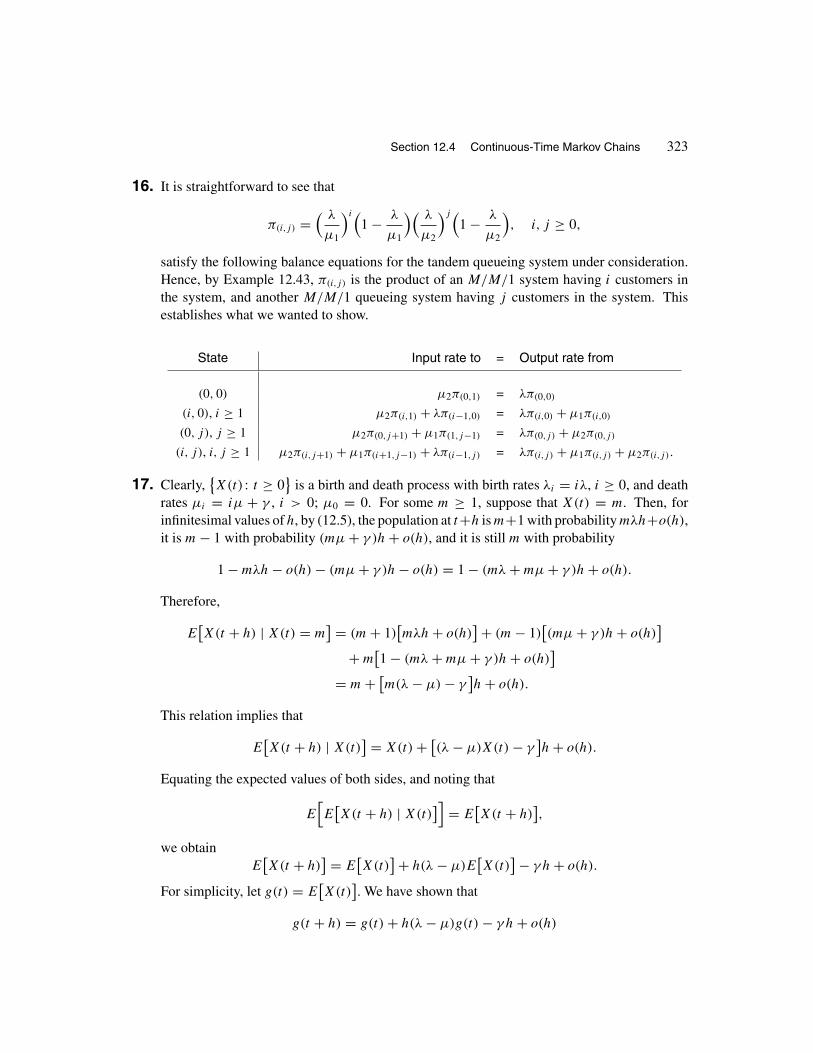
Section 12.4 Continuous-Time Markov Chains 323
16. It is straightforward to see that
π(i,j) =( λ
µ1
)i(1 − λ
µ1
)( λ
µ2
)j(1 − λ
µ2
), i, j ≥ 0,
satisfy the following balance equations for the tandem queueing system under consideration.Hence, by Example 12.43, π(i,j) is the product of an M/M/1 system having i customers inthe system, and another M/M/1 queueing system having j customers in the system. Thisestablishes what we wanted to show.
State Input rate to = Output rate from
(0, 0) µ2π(0,1) = λπ(0,0)
(i, 0), i ≥ 1 µ2π(i,1) + λπ(i−1,0) = λπ(i,0) + µ1π(i,0)
(0, j), j ≥ 1 µ2π(0,j+1) + µ1π(1,j−1) = λπ(0,j) + µ2π(0,j)
(i, j), i, j ≥ 1 µ2π(i,j+1) + µ1π(i+1,j−1) + λπ(i−1,j) = λπ(i,j) + µ1π(i,j) + µ2π(i,j).
17. Clearly,{X(t) : t ≥ 0
}is a birth and death process with birth rates λi = iλ, i ≥ 0, and death
rates µi = iµ + γ , i > 0; µ0 = 0. For some m ≥ 1, suppose that X(t) = m. Then, forinfinitesimal values of h, by (12.5), the population at t+h is m+1 with probability mλh+o(h),it is m − 1 with probability (mµ + γ )h + o(h), and it is still m with probability
1 − mλh − o(h) − (mµ + γ )h − o(h) = 1 − (mλ + mµ + γ )h + o(h).
Therefore,
E[X(t + h) | X(t) = m
] = (m + 1)[mλh + o(h)
]+ (m − 1)[(mµ + γ )h + o(h)
]+ m
[1 − (mλ + mµ + γ )h + o(h)
]= m + [
m(λ − µ) − γ]h + o(h).
This relation implies that
E[X(t + h) | X(t)
] = X(t) + [(λ − µ)X(t) − γ
]h + o(h).
Equating the expected values of both sides, and noting that
E[E[X(t + h) | X(t)
]] = E[X(t + h)
],
we obtainE[X(t + h)
] = E[X(t)
]+ h(λ − µ)E[X(t)
]− γ h + o(h).
For simplicity, let g(t) = E[X(t)
]. We have shown that
g(t + h) = g(t) + h(λ − µ)g(t) − γ h + o(h)

324 Chapter 12 Stochastic Processes
or, equivalently,g(t + h) − g(t)
h= (λ − µ)g(t) − γ + o(h)
h.
As h → 0, this givesg′(t) = (λ − µ)g(t) − γ.
If λ = µ, then g′(t) = −γ . So g(t) = −γ t + c. Since g(0) = n, we must have c = n, org(t) = −γ t + n. If λ �= µ, to solve the first order linear differential equation,
g′(t) = (λ − µ)g(t) − γ,
let f (t) = (λ − µ)g(t) − γ. Then
1
λ − µf ′(t) = f (t),
orf ′(t)f (t)
= λ − µ.
This yieldsln |f (t)| = (λ − µ)t + c,
orf (t) = e(λ−µ)t+c = Ke(λ−µ)t ,
where K = ec. Thus
g(t) = K
λ − µe(λ−µ)t + γ
λ − µ.
Now g(0) = n implies that K = n(γ − µ) − γ. Thus
g(t) = E[X(t)
] = ne(λ−µ)t + γ
λ − µ
[1 − e(λ−µ)t
].
18. For n ≥ 0, let En be the event that, starting from state n, eventually extinction will occur. Letαn = P(En). Clearly, α0 = 1. We will show that αn = 1, for all n. For n ≥ 1, starting fromn, let Zn be the state to which the process will move. Then Zn is a discrete random variablewith set of possible values {n − 1, n + 1}. Conditioning on Zn yields
P(En) = P(En | Zn = n − 1)P (Zn = n − 1) + P(En | Zn = n + 1)P (Zn = n + 1).
Hence
αn = αn−1 · µn
λn + µn
+ αn+1 · λn
λn + µn
, n ≥ 1,
or, equivalently,λn(αn+1 − αn) = µn(αn − αn−1), n ≥ 1.

Section 12.4 Continuous-Time Markov Chains 325
For n ≥ 0, let yn = αn+1 − αn. We have
λnyn = µnyn−1, n ≥ 1,
oryn = µn
λn
yn−1, n ≥ 1.
Therefore,
y1 = µ1
λ1y0
y2 = µ2
λ2y1 = µ1µ2
λ1λ2y0
...
yn = µ1µ2 · · · µn
λ1λ2 · · · λn
y0. n ≥ 1.
On the other hand, by yn = αn+1 − αn, n ≥ 0,
α1 = α0 + y0 = 1 + y0
α2 = α1 + y1 = 1 + y0 + y1
...
αn+1 = 1 + y0 + y1 + · · · + yn.
Hence
αn+1 = 1 + y0 +n∑
k=1
yk
= 1 + y0 + y0
n∑k=1
µ1µ2 · · · µk
λ1λ2 · · · λk
= 1 + y0
(1 +
n∑k=1
µ1µ2 · · · µk
λ1λ2 · · · λk
)
= 1 + (α1 − 1)(
1 +n∑
k=1
µ1µ2 · · · µk
λ1λ2 · · · λk
).
Since∞∑
k=1
µ1µ2 · · · µk
λ1λ2 · · · λk
= ∞, the sequencen∑
k=1
µ1µ2 · · · µk
λ1λ2 · · · λk
increases without bound. For
αn’s to exist, this requires that α1 = 1, which in turn implies that αn+1 = 1, for n ≥ 1.

326 Chapter 12 Stochastic Processes
12.5 BROWNIAN MOTION
1. (a) By the independent-increments property of Brownian motions, the desired probabilityis
P(− 1/2 < Z(10) < 1/2 | Z(5) = 0
)= P
(− 1/2 < Z(10) − Z(5) < 1/2 | Z(5) = 0)
= P(− 1/2 < Z(10) − Z(5) < 1/2
).
Since Z(10) − Z(5) is normal with mean 0 and variance (10 − 5)σ 2 = 45, lettingZ ∼ N(0, 1), we have
P(− 1/2 < Z(10) − Z(5) < 1/2
)= P
(−0.5 − 0√45
< Z <0.5 − 0√
45
)≈ P(−0.07 < Z < 0.07) = �(0.07) − �(−0.07) = 0.056.
(b) In Theorem 12.9, let t1 = 5, t2 = 7, z1 = 0, z2 = −1. We have
E[Z(6) | Z(5) = 0 and Z(7) = −1
] = 0 + −1 − 0
7 − 5(6 − 5) = −0.5,
Var[Z(6) | Z(5) = 0 and Z(7) = −1
] = 9 · (7 − 6)(6 − 5)
7 − 5= 4.5.
2. In the subsection of 12.5, The Maximum of a Brownian Motion, we have shown that
P(
max0≤s≤t
X(s) ≤ u) =
⎧⎨⎩2�( u
σ√
t
)− 1 u ≥ 0
0 u < 0.
We will show that |X(t)| has the same probability distribution function. To do so, note thatX(t) ∼ N(0, σ 2t) and X(t)/(σ
√t) is standard normal. Thus, for u ≥ 0,
P(|X(t)| ≤ u
) = P(− u ≤ X(t) ≤ u
) = P(X(t) ≤ u
)− P(X(t) < −u
)= P
(Z ≤ u
σ√
t
)− P
(Z < − u
σ√
t
)= �
( u
σ√
t
)−[1 − �
( u
σ√
t
)]= 2�
( u
σ√
t
)− 1.
For u < 0, P(|X(t)| ≤ u
) = 0. Hence max0≤s≤t
X(s) and |X(t)| are identically distributed.
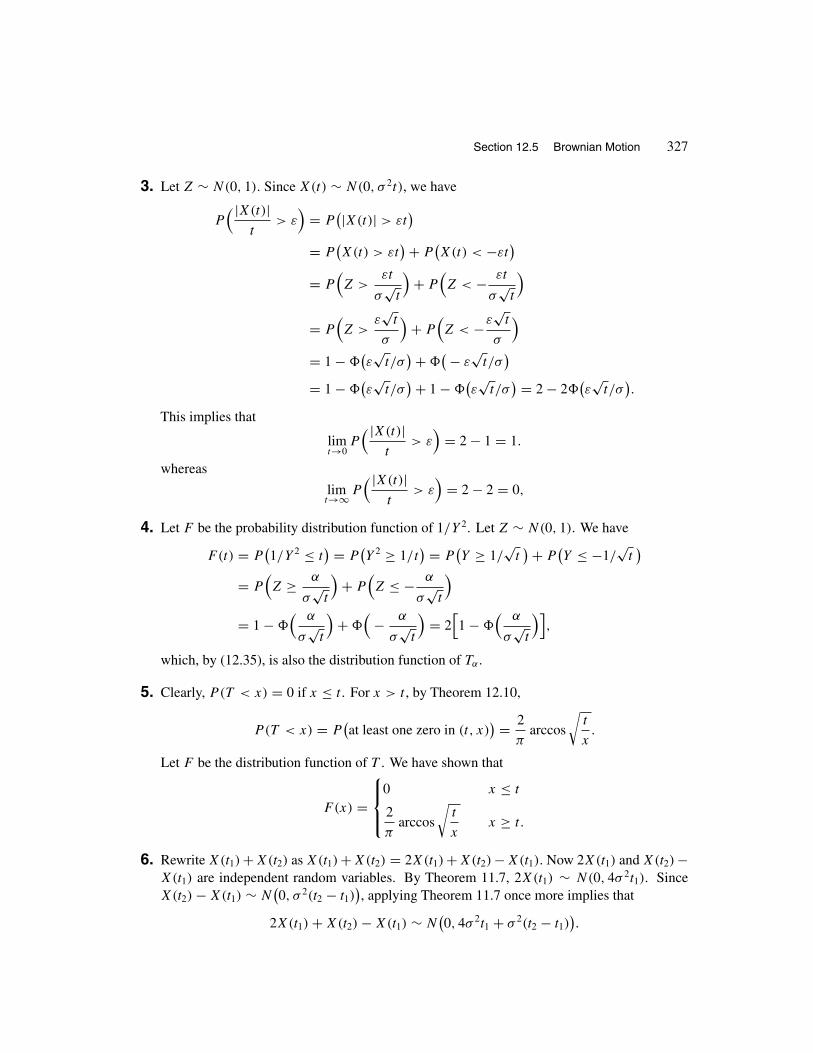
Section 12.5 Brownian Motion 327
3. Let Z ∼ N(0, 1). Since X(t) ∼ N(0, σ 2t), we have
P( |X(t)|
t> ε
)= P
(|X(t)| > εt)
= P(X(t) > εt
)+ P(X(t) < −εt
)= P
(Z >
εt
σ√
t
)+ P
(Z < − εt
σ√
t
)= P
(Z >
ε√
t
σ
)+ P
(Z < −ε
√t
σ
)= 1 − �
(ε√
t/σ)+ �
(− ε√
t/σ)
= 1 − �(ε√
t/σ)+ 1 − �
(ε√
t/σ) = 2 − 2�
(ε√
t/σ).
This implies that
limt→0
P( |X(t)|
t> ε
)= 2 − 1 = 1.
whereas
limt→∞ P
( |X(t)|t
> ε)
= 2 − 2 = 0,
4. Let F be the probability distribution function of 1/Y 2. Let Z ∼ N(0, 1). We have
F(t) = P(1/Y 2 ≤ t
) = P(Y 2 ≥ 1/t
) = P(Y ≥ 1/
√t)+ P
(Y ≤ −1/
√t)
= P(Z ≥ α
σ√
t
)+ P
(Z ≤ − α
σ√
t
)= 1 − �
( α
σ√
t
)+ �
(− α
σ√
t
)= 2
[1 − �
( α
σ√
t
)],
which, by (12.35), is also the distribution function of Tα.
5. Clearly, P(T < x) = 0 if x ≤ t . For x > t , by Theorem 12.10,
P(T < x) = P(at least one zero in (t, x)
) = 2
πarccos
√t
x.
Let F be the distribution function of T . We have shown that
F(x) =
⎧⎪⎨⎪⎩0 x ≤ t
2
πarccos
√t
xx ≥ t.
6. Rewrite X(t1) + X(t2) as X(t1) + X(t2) = 2X(t1) + X(t2) − X(t1). Now 2X(t1) and X(t2) −X(t1) are independent random variables. By Theorem 11.7, 2X(t1) ∼ N(0, 4σ 2t1). SinceX(t2) − X(t1) ∼ N
(0, σ 2(t2 − t1)
), applying Theorem 11.7 once more implies that
2X(t1) + X(t2) − X(t1) ∼ N(0, 4σ 2t1 + σ 2(t2 − t1)
).

328 Chapter 12 Stochastic Processes
Hence X(t1) + X(t2) ∼ N(0, 3σ 2t1 + σ 2t2).
7. Let f (x, y) be the joint probability density function of X(t) and X(t+u). Let fX(t+u)|X(t)(y|a)
be the conditional probability density function of X(t + u) given that X(t) = a. Let fX(t)(x)
be the probability density function of X(t). We know that X(t) is normal with mean 0 andvariance σ 2t . The formula for f (x, y) is given by (12.28). Using these, we obtain
fX(t+u)|X(t)(y|a) = f (a, y)
fX(t)(a)=
1
2σ 2π√
tuexp
(− 1
2σ 2
[a2
t+ (y − a)2
u
])1
σ√
2πtexp
(− a2
2σ 2t
)= 1
σ√
2πuexp
[− 1
2σ 2u(y − a)2
].
This shows that the conditional probability density function of X(t + u) given that X(t) = a
is normal with mean a and variance σ 2u. Hence
E[X(t + u) | X(t) = a
] = a.
This implies that
E[X(t + u) | X(t)
] = X(t).
8. By Example 10.23,
E[X(t)X(t + u) | X(t)
] = X(t)E[X(t + u) | X(t)
].
By Exercise 7 above,
E[X(t + u) | X(t)
] = X(t).
Hence
E[X(t)X(t + u)
] = E[E[X(t)X(t + u) | X(t)
]= E
[X(t)E
[X(t + u) | X(t)
]]= E
[X(t) · X(t)
] = E[X(t)2
]= Var
[X(t)
]+ (E[X(t)
])2 = σ 2t + 0 = σ 2t.
9. For t > 0, the probability density function of Z(t) is
φt(x) = 1
σ√
2πtexp
[− x2
2σ 2t
].

Section 12.5 Brownian Motion 329
Therefore,
E[V (t)
] = E[|Z(t)|] =
∫ ∞
−∞|x|φt(x) dx
= 2∫ ∞
0xφt(x) dx = 2
∫ ∞
0
x
σ√
2πte−x2/(2σ 2t) dx.
Making the change of variable u = x
σ√
tyields
E[V (t)
] = σ
√2t
π
∫ ∞
0ue−u2/2 du = σ
√2t
π
[− e−u2/2
]∞0
= σ
√2t
π.
Var[V (t)
] = E[V (t)2
]− (E[V (t)
])2 = E[Z(t)2
]− 2σ 2t
π
= σ 2t − 2σ 2t
π= σ 2t
(1 − 2
π
),
since
E[Z(t)2
] = Var[Z(t)
]+ (E[Z(t)
])2 = σ 2t + 0 = σ 2t.
To find P(V (t) ≤ z | V (0) = z0
), note that, by (12.27),
P(V (t) ≤ z | V (0) = z0
) = P(|Z(t)| ≤ z | V (0) = z0
)= P
(− z ≤ Z(t) ≤ z | V (0) = z0)
=∫ z
−z
1
σ√
2πte−(u−z0)
2/(2σ 2t) du.
Letting U ∼ N(z0, σ2t) and Z ∼ N(0, 1), this implies that
P(V (t) ≤ z | V (0) = z0
) = P(−z ≤ U ≤ z)
= P(−z − z0
σ√
t≤ z ≤ z − z0
σ√
t
)= �
(z − z0
σ√
t
)− �
(−z − z0
σ√
t
)= �
(z + z0
σ√
t
)+ �
(z − z0
σ√
t
)− 1.
10. Clearly, D(t) = √X(t)2 + Y (t)2 + Z(t)2. Since X(t), Y (t), and Z(t) are independent and

330 Chapter 12 Stochastic Processes
identically distributed normal random variables with mean 0 and variance σ 2t , we have
E[D(t)
] =∫ ∞
−∞
∫ ∞
−∞
∫ ∞
−∞
√x2 + y2 + z2 · 1
σ√
2πte−x2/(2σ 2t) · 1
σ√
2πte−y2/(2σ 2t)
· 1
σ√
2πte−z2/(2σ 2t) dx dy dz
= 1
2πσ 3t√
2πt
∫ ∞
−∞
∫ ∞
−∞
∫ ∞
−∞
√x2 + y2 + z2 · e−(x2+y2+z2)/(2σ 2t) dx dy dz.
We now make a change of variables to spherical coordinates: x = ρ sin φ cos θ , y =ρ sin φ sin θ , z = ρ cos φ, ρ2 = x2 + y2 + z2, dx dy dz = ρ2 sin φ dρ dφ dθ, 0 ≤ ρ < ∞,
0 ≤ φ ≤ π , and 0 ≤ θ ≤ 2π . We obtain
E[D(t)
] = 1
2πσ 3t√
2πt
∫ 2π
0
∫ π
0
∫ ∞
0ρe−ρ2/(2σ 2t) · ρ2 sin φ dρ dφ, dθ
= 1
2πσ 3t√
2πt
∫ 2π
0
[ ∫ π
0
( ∫ ∞
0ρ3e−ρ2/(2σ 2t) dρ
)sin φ dφ
]dθ
= 1
2πσ 3t√
2πt
∫ 2π
0
( ∫ π
0
[− σ 2t (ρ2 + 2σ 2t)e−ρ2/(2σ 2t)
]∞0
sin φ dφ)
dθ
= 1
2πσ 3t√
2πt· 2σ 4t2
∫ 2π
0
( ∫ π
0sin φ dφ
)dθ = 2σ
√2t
π.
11. Noting that√
5.29 = 2.3, we have
V (t) = 95e−2t+2.3W(t),
where{W(t) : t ≥ 0
}is a standard Brownian motion. Hence W(t) ∼ N(0, t). The desired
probability is
P(V (0.75) < 80
) = P(95e−2(0.75)+2.3W(0.75) < 80
)= P
(e2.3W(0.75) < 3.774
) = P(W(0.75) < 0.577
)= P
(W(0.75) − 0√0.75
<0.577√
0.75
)= P(Z < 0.67) = �(0.67) = 0.7486.

Chapter 12 Review Problems 331
REVIEW PROBLEMS FOR CHAPTER 12
1. Label the time point 10:00 as t = 0. We are given that N(180) = 10 and are interested inP(S10 ≥ 160 | N(180) = 10
). Let X1, X2, . . . , X10 be 10 independent random variables uni-
formly distributed over the interval [0, 180]. Let Y = max(X1, . . . , X10). By Theorem 12.4,
P(S10 > 160 | N(180) = 10
) = P(Y > 160) = 1 − P(Y ≤ 160)
= 1 − P(
max(X1, . . . , X10) ≤ 160)
= 1 − P(X1 ≤ 160)P (X2 ≤ 160) · · · P(X10 ≤ 160)
= 1 −(160
180
)10 = 0.692.
2. For all positive integer n, we have that
P 2n =(
1 00 1
)and P 2n+1 =
(0 11 0
).
Therefore, {Xn : n = 0, 1, . . . } is not regular.
3. By drawing a transition graph, it can be readily seen that, if states 0, 1, 2, 3, and 4 are renamed0, 4, 2, 1, and 3, respectively, then the transition probability matrix P 1 will change to P 2.
4. Let Z be the number of transitions until the first visit to 1. Clearly, Z is a geometric randomvariable with parameter p = 3/5. Hence its expected value is 1/p = 5/3.
5. By drawing a transition graph, it is readily seen that this Markov chain consists of two recurrentclasses {3, 5} and {4}, and two transient classes {1} and {2}.
6. We have that
Xn+1 ={
Xn if the (n + 1)st outcome is not 6
1 + Xn if the (n + 1)st outcome is 6.
This shows that {Xn : n = 1, 2, . . . } is a Markov chain with state space {0, 1, 2, . . . }. Itstransition probability matrix is given by
P =
⎛⎜⎜⎜⎜⎜⎝5/6 1/6 0 0 0 . . .
0 5/6 1/6 0 0 . . .
0 0 5/6 1/6 0 . . .
0 0 0 5/6 1/6 . . ....
⎞⎟⎟⎟⎟⎟⎠ .
All states are transient; no two states communicate with each other. Therefore, we haveinfinitely many classes; namely, {0}, {1}, {2}, . . . , and each one of them is transient.

332 Chapter 12 Stochastic Processes
7. The desired probability is
p11p11 + p11p12 + p12p22 + p12p21 + p21p11 + p21p12 + p22p21 + p22p22
= (0.20)2 + (0.20)(0.30) + (0.30)(0.15) + (0.30)(0.32)
+ (0.32)(0.20) + (0.32)(0.30) + (0.15)(0.32) + (0.15)2 = 0.4715.
8. The following is an example of such a transition probability matrix:
P =
⎛⎜⎜⎜⎜⎜⎜⎜⎜⎜⎜⎝
0 0 1 0 0 0 0 01 0 0 0 0 0 0 00 0 0 1 0 0 0 00 1/2 0 0 1/2 0 0 00 0 0 0 1/3 2/3 0 00 0 0 0 0 0 1 00 0 0 0 0 0 0 10 0 0 0 0 1 0 0
⎞⎟⎟⎟⎟⎟⎟⎟⎟⎟⎟⎠.
9. For n ≥ 1, let
Xn ={
1 if the nth golfball produced is defective
0 if the nth golfball produced is good.
Then {Xn : n = 1, 2, . . . } is a Markov chain with state space {0, 1} and transition probability
matrix(
15/18 3/1811/12 1/12
). Let π0 be the fraction of golfballs produced that are good, and π1 be
the fraction of the balls produced that are defective. Then, by Theorem 12.7, π0 and π1 satisfy(π0
π1
)=(
15/18 11/123/18 1/12
)(π0
π1
),
which gives us the following system of equations⎧⎨⎩π0 = (15/18)π0 + (11/12)π1
π1 = (3/18)π0 + (1/12)π1.
By choosing any one of these equations along with the relation π0 + π1 = 1, we obtain asystem of two equations in two unknowns. Solving that system yields
π0 = 11
13≈ 0.85 and π1 = 2
13≈ 0.15.
Therefore, approximately 15% of the golfballs produced have no logos.
10. Let
Xn =
⎧⎪⎨⎪⎩1 if the nth ball is drawn by Carmela
2 if the nth ball is drawn by Daniela
3 if the nth ball is drawn by Lucrezia.

Chapter 12 Review Problems 333
The process {Xn : n = 1, 2, . . . } is an irreducible, aperiodic, positive recurrent Markov chainwith transition probability matrix
P =⎛⎝7/31 11/31 13/31
7/31 11/31 13/317/31 11/31 13/31
⎞⎠ .
Let π1, π2, and π3 be the long-run proportion of balls drawn by Carmela, Daniela, and Lucrezia,respectively. Intuitively, it should be clear that these quantities are 7/31, 11/31, and 13/31,respectively. However, that can be seen also by solving the following matrix equation alongwith π0 + π1 + π3 = 1.⎛⎝π1
π2
π3
⎞⎠ =⎛⎝ 7/31 7/31 7/31
11/31 11/31 11/3113/31 13/31 13/31
⎞⎠⎛⎝π1
π2
π3
⎞⎠ .
11. Let π1 and π2 be the long-run probabilities that Francesco devotes to playing golf and playingtennis, respectively. Then, by Theorem 12.7, π1 and π2 are obtained from solving the systemof equations (
π1
π2
)=(
0.30 0.580.70 0.42
)(π1
π2
)along with π1 + π2 = 1. The matrix equation above gives the following system of equations:{
π1 = 0.30π1 + 0.58π2
π2 = 0.70π1 + 0.42π2.
By choosing any one of these equations along with the relation π1 + π2 = 1, we obtaina system of two equations in two unknowns. Solving that system yields π1 = 0.453125and π2 = 0.546875. Therefore, the long-run probability that, on a randomly selected day,Francesco plays tennis is approximately 0.55.
12. Suppose that a train leaves the station at t = 0. Let X1 be the time until the first passengerarrives at the station after t = 0. Let X2 be the additional time it will take until a train arrivesat the station, X3 be the time after that until a passenger arrives, and so on. Clearly, X1,X2, . . . are the times between consecutive change of states. By the memoryless propertyof exponential random variables, {X1, X2, . . . } is a sequence of independent and identicallydistributed exponential random variables with mean 1/λ. Hence, by Remark 7.2,
{N(t) : t ≥
0}
is a Poisson process with rate λ. Therefore, N(t) is a Poisson random variable withparameter λt .
13. Let X(t) be the number of components working at time t . Clearly,{X(t) : t ≥ 0
}is a
continuous-time Markov chain with state space {0, 1, 2}. Let π0, π1, and π2 be the long-runproportion of time the process is in states 0, 1, and 2, respectively. The balance equations for{X(t) : t ≥ 0
}are as follows:

334 Chapter 12 Stochastic Processes
State Input rate to = Output rate from
0 λπ1 = µπ0
1 2λπ2 + µπ0 = µπ1 + λπ1
2 µπ1 = 2λπ2
From these equations, we obtain π1 = µ
λπ0 and π2 = µ2
2λ2π0. Using π0 + π1 + π2 = 1 yields
π0 = 2λ2
2λ2 + 2λµ + µ2.
Hence the desired probability is
1 − π0 = µ(2λ + µ)
2λ2 + 2λµ + µ2.
14. Suppose that every time an out-of-order machine is repaired and is ready to operate a birthoccurs. Suppose that a death occurs every time that a machine breaks down. The fact that{X(t) : t ≥ 0
}is a birth and death process should be clear. The birth and death rates are
λn =
⎧⎪⎪⎨⎪⎪⎩kλ n = 0, 1, . . . , m + s − k
(m + s − n)λ n = m + s − k + 1, m + s − k + 2, . . . , m + s
0 n ≥ m + s;
µn =
⎧⎪⎪⎨⎪⎪⎩nµ n = 0, 1, . . . , m
mµ n = m + 1, m + 2, . . . , m + s
0 n > m + s.
15. Let X(t) be the number of machines operating at time t . For 0 ≤ i ≤ m, let πi be the long-runproportion of time that there are exactly i machines operating. Suppose that a birth occurseach time that an out-of-order machine is repaired and begins to operate, and a death occurseach time that a machine breaks down. Then
{X(t) : t ≥ 0
}is a birth and death process with
state space {0, 1, . . . , m}, and birth and death rates, respectively, given by λi = (m − i)λ andµi = iµ for i = 0, 1, . . . , m. To find π0, first we will calculate the following sum:
m∑i=1
λ0λ1 · · · λi−1
µ1µ2 · · · µi
=m∑
i=1
(mλ)[(m − 1)λ
][(m − 2)λ
] · · · [(m − i + 1)λ]
µ(2µ)(3µ) · · · (iµ)
=m∑
i=1
mPi λi
i! µi=
m∑i=1
(m
i
)( λ
µ
)i
= −1 +m∑
i=0
(m
i
)( λ
µ
)i
1m−i = −1 +(
1 + λ
µ
)m
,

Chapter 12 Review Problems 335
where mPi is the number of i-element permutations of a set containing m objects. Hence, by(12.22),
π0 =(
1 + λ
µ
)−m =(λ + µ
µ
)−m =( µ
λ + µ
)m
.
By (12.21),
πi = λ0λ1 · · · λi−1
µ1µ2 · · · µi
π0 = mPiλi
i! µiπ0
=(
m
i
)( λ
µ
)i( µ
λ + µ
)m =(
m
i
)( λ
µ
)i( µ
λ + µ
)i( µ
λ + µ
)m−i
=(
m
i
)( λ
λ + µ
)i(1 − λ
λ + µ
)m−i
, 0 ≤ i ≤ m.
Therefore, in steady-state, the number of machines that are operating is binomial with param-eters m and λ/(λ + µ).
16. Let X(t) be the number of cars at the center, either being inspected or waiting to be inspected,at time t . Clearly,
{X(t) : t ≥ 0
}is a birth and death process with rates λn = λ/(n + 1),
n ≥ 0, and µn = µ, n ≥ 1. Since
∞∑n=1
λ0λ1 · · · λn−1
µ1µ2 · · · µn
=∞∑
n=1
λ · λ
2· λ
3· · · λ
n
µn= −1 +
∞∑n=0
1
n!( λ
µ
)n = eλ/µ − 1.
By (12.18), π0 = e−λ/µ. Hence, by (12.17),
πn =λ · λ
2· λ
3· · · λ
n
µne−λ/µ = (λ/µ)ne−λ/µ
n! , n ≥ 0.
Therefore, the long-run probability that there are n cars at the center for inspection is Poissonwith rate λ/µ.
17. Let X(t) be the population size at time t . Then{X(t) : t ≥ 0
}is a birth and death process with
birth rates λn = nλ, n ≥ 1, and death rates µn = nµ, n ≥ 0. For i ≥ 0, let Hi be the time,starting from i, until the population size reaches i + 1 for the first time. We are interested in∑4
i=1 E(Hi). Note that, by Lemma 12.2,
E(Hi) = 1
λi
+ µi
λi
E(Hi−1), i ≥ 1.
Since E(H0) = 1/λ,
E(H1) = 1
λ+ µ
λ· 1
λ= 1
λ+ µ
λ2,

336 Chapter 12 Stochastic Processes
E(H2) = 1
2λ+ 2µ
2λ·(1
λ+ µ
λ2
)= 1
2λ+ µ
λ2+ µ2
λ3,
E(H3) = 1
3λ+ 3µ
3λ
( 1
2λ+ µ
λ2+ µ2
λ3
)= 1
3λ+ µ
2λ2+ µ2
λ3+ µ3
λ4,
E(H4) = 1
4λ+ 4µ
4λ
( 1
3λ+ µ
2λ2+ µ2
λ3+ µ3
λ4
)= 1
4λ+ µ
3λ2+ µ2
2λ3+ µ3
λ4+ µ4
λ5.
Therefore, the answer is
4∑i=1
E(Hi) = 25λ4 + 34λ3µ + 30λ2µ2 + 24λµ3 + 12µ4
12λ5.
18. Let X(t) be the population size at time t . Then{X(t) : t ≥ 0
}is a birth and death process
with rates λn = γ, n ≥ 0, and µn = nµ, n ≥ 1. To find πi’s, we will first calculate the sumin the relation (12.18):
∞∑n=1
λ0λ1 · · · λn−1
µ1µ2 · · · µn
=∞∑
n=1
γ n
n! µn= −1 +
∞∑n=0
1
n!(γ
µ
)n = −1 + eγ/µ.
Thus, by (12.18), π0 = e−γ /µ and, by (12.17), for i ≥ 1,
πi = γ n
n! µne−γ /µ = (γ /µ)ne−γ /µ
n! .
Hence the steady-state probability mass function of the population size is Poisson with pa-rameter γ /µ.
19. By applying Theorem 12.9 to{Y (t) : t ≥ 0
}with t1 = 0, t2 = t , y1 = 0, y2 = y, and t = s,
we have
E[Y (s) | Y (t) = y
] = 0 + y − 0
t − 0(s − 0) = s
ty,
and
Var[Y (s) | Y (t) = y
] = σ 2 · (t − s)(s − 0)
t − 0= σ 2(t − s)
s
t.
20. First, suppose that s < t . By Example 10.23,
E[X(s)X(t) | X(s)
] = X(s)E[X(t) | X(s)
].
Now, by Exercise 7, Section 12.5,
E[X(t) | X(s)
] = X(s).

Chapter 12 Review Problems 337
Hence
E[X(s)X(t)
] = E[E[X(s)X(t) | X(s)
]]= E
[X(s)E
[X(t) | X(s)
]]= E
[X(s)X(s)
] = E[X(s)2
]= Var
[X(s)
]+ (E[X(s)
])2
= σ 2s + 0 = σ 2s.
For t < s, by symmetry,E[X(s)X(t)
] = σ 2t.
Therefore,E[X(s)X(t)
] = σ 2 min(s, t).
21. By Theorem 12.10,
P(U < x and T > y) = P(no zeros in (x, y)
) = 1 − 2
πarccos
√x
y.
22. Let the current price of the stock, per share, be v0. Noting that√
27.04 = 5.2, we have
V (t) = v0e3t+5.2W(t),
where{W(t) : t ≥ 0
}is a standard Brownian motion. Hence W(t) ∼ N(0, t). The desired
probability is calculated as follows:
P(V (2) ≥ 2v0
) = P(v0e
6+5.2W(2) ≥ 2v0)
= P(6 + 5.2W(2) ≥ ln 2
) = P(W(2) ≥ −1.02
)= P
(W(2) − 0√2
≥ −0.72)
= P(Z ≥ −0.72) = 1 − P(Z < −0.72)
= 1 − �(−0.72) = 0.7642.