International Journal Of Computational Engineering Research (ijceronline.com) Vol. 2 Issue. 8

||Issn 2250-3005(online)|| ||December|| 2012 Page 297

Fundamental Theorem Of Algebra A Study

Dr Mushtaq Ahmad Shah Department of Mathematics CMJ University Shilliong 79300

Abstract: This paper is a study of the Fundamental Theorem of A lgebra which states that every polynomial equation of

degree n has exactly n zeroes. It gives a historical account of the theorem in different periods; by different mathemat icians it

also includes the contribution of different countries. In addition to this I present different proofs of Fundamental Theorem of

Algebra by using different techniques which is actually the main theme behind the paper.

Keywords:- Polynomials, zeroes, analytic, bounded, constant, Maximum Modulus,

1. Introduction When we speak of the early history of algebra, first of all it is necessary to consider the meaning of the term. If by

algebra we mean the science which allows us to solve the equation ax2 + bx + c = 0, expressed in these symbols, then the

history begins in the 17th

Century ; if we remove the restrictions as to these particular signs and allow for other and less

convenient symbols. we might properly begins the history in the 3rd

century ; if we allow for the solution of the above equation

by geometric methods, without algebraic symbols of any kind, we might say that the algebra begins with the A lexandrian

School or a little earlier; and if we say we should class as algebra any problem that we should now solve by algebra ( even

through it was at first solved by mere guessing or by some cumbersome arithmet ic process), then the science was known abo ut

I800 B.C,, and probably still earlier. It is first proposed to give a brief survey of the development of algebra, recalling t he

names of those who helped to set the problems that were later solved by the aid of equation, as well as those who assisted in

establishing the science itself. These names have been mentioned in Volume 1 and some of them will be referred to when we

consider the development of the special topics of algebra and their application to the solution of the elementary problems. I t

should be borne in mind that most ancient writers outside Greece included in their mathematics works a wide range of

subjects. Ahmes (c.1550 B.C.), for example, combines his algebra with arithmetic and mensuration, and even shows some

evidence that trigonometry was making a feeble start. There was no distinct treatise on algebra before the time of Diophantus

(c.275). There are only four Hindu writers on algebra whose are particularly noteworthy. These are Aryabhata, whose

Aryabha-tiyam(c.510) included problems in series, permutation , and linear and quadratic equations; Brahmagupta, whose

Brahmasid-dhanta(c.628) contains a satisfactory rule for the solving the quadratic, and whose problems included the subjects

treated by Aryabhata : Mahavira whose Ganita -Sari Sangraha (c.850) contains a large number of p roblems involving series,

radicals, and equations; and Bhaskara, whose Bija Ganita (c.1150) contains nine chapters and extended the work through

quadratic equations.

Algebra in the modern sense can hardly be said to have existed in the golden age of Greek mathemat ics. The Greeks

of the classical period could solve many algebraic problems of considerable difficulty, but the solutions were all geometric.

Hippocrates (c.460 B.C.), for example, assumed a construction which is equivalent to solving the equation

22

2

3aaxx .

With Diophantus (c.275) there first enters an algebraic symbolis m worthy of the name, and also a series of purely

algebraic problems treated by analytic methods. Many of his equations being indeterminate, equation of this type are often

called Diophantine Equations. His was the first work devoted chiefly to algebra, and on his account he is often, and with mus t

justice, called the father of the science. The algebraists of special prominence among the Arabs and Persians were Mohammed

ibn Musa, al- Khowarizmi, whose al- jabr w‟al muqabalah(c.825) gave the name to the science and contained the first

systematic treatment of the general subject as distinct from the theory of numbers; Almahani (c.860), whose name will be

mentioned in connection with the cubic; Abu kamil (c.900), who drew extensively from al - khawarizmi and from whom

Fibonacci (1202) drew in turn; al-Karkh i(c.1020), whose Fakhri contains various problems which still form part of the general

stock material of algebra; and Omar Khanyyam (c.1100), whose algebra was the best that the Persian writers produced.

Most of the medieval Western scholars who helped in the progress of algebra were translators from the Arabic.

Among these were Johannes Hispalensis (c.1140), who may have translated al-Khowarizmi‟s algebra; Gherardo of Cremona

(c.1150), to whom is also attributed a translation of the same work; Adelard of Bath (c.1120), who probably translated an

asronomical work of al-Khowarizmi, and who certainly helped to make this writer Known; and Robert of Chester, whose

translation of al-Khoarizmi‟s algebra is now availab le in English.

International Journal Of Computational Engineering Research (ijceronline.com) Vol. 2 Issue. 8

||Issn 2250-3005(online)|| ||December|| 2012 Page 298

The first epoch-making algebra to appear in print was the Ars Magna of Cardan (1545). This was devoted primarily

to the solutions of algebraic equations. It contained the solutions of the cubic and biquadratic equations, made use of complex

numbers, and in general may be said to have been the first step towards modern algebra.The next g reat work on algebra to

appear in print was the General Trattato of Tartaglia (1556-1560), although his side of the controversy with Cardan over the

solution of the cubic equation had already been given in his qvesitised inventioni diverse (1546). The first noteworthy attempt

to write algebra in England was made by Robert Recorde, who Whetstone of Witte (1557) was an excellent textbook for its

first time. The next important contribution was Masterson‟s incomplete treatise of 1592 -1595, but the work was not up to

standard set by Recorde. The first Italian textbook to bear the title of algebra was Bombelli‟s work of 1572. In this book t he

material is arranged with some attention to the teaching of the subject.

By this time elementary algebra was fairly well perfected and it only remained to develop a good symbolism. Every

real polynomial can be expressed as the product of real linear and real quadratic factors.Early studies of equations by al-

Khwarizmi (c 800) only allowed positive real roots and the Fundamental Theorem of Algebra was not relevant. Cardan

was the first to realise that one could work with quantities more general than the real numbers. This discovery was

made in the course of studying a formula which gave the roots of a cubic equation. The formula when applied to the

equation x3 = 15x + 4 gave an answer involving √-121 yet Cardan knew that the equation had x = 4 as a solution. He

was able to manipulate with his 'complex numbers' to obtain the right answer yet he in no way unde rstood his own

mathematics. Bombelli, in his Algebra, published in 1572, was to produce a proper set of rules for manipulating these

„complex numbers'. Descartes in 1637 says that one can 'imagine' for every equation of degree n, n roots but these

imagined roots do not correspond to any real quantity Viète gave equations of degree n with n roots but the first claim

that there are always n solutions was made by a Flemish mathemat ician Albert Girard in 1629 in L'invention en algebre

However he does not assert that solutions are of the form a + bi, a, b real, so allows the possibility that solutions

come from a larger number field than C. In fact this was to become the whole problem of the Fundamental Theorem

of Algebra for many years since mathematicians accepted Albert Girard's assertion as self-evident. They believed that

a polynomial equation of degree n must have n roots, the problem was, they believed, to show that these roots were

of the form a + bi, a, b real Now Harriot knew that a polynomial which vanishes at t has a root x - t but this did

not become well known until stated by Descartes in 1637 in La geometrie, so Albert Girard did not have much of the

background to understand the problem properly.

A 'proof' that the Fundamental Theorem of A lgebra was false was given by Leibniz in 1702 when he asserted

that x4 + t

4 could never be written as a product of two real quadratic factors. His mistake came in not realizing that

√i could be written in the form a + bi, a, b real. Euler, in a 1742 correspondence with Nico laus(II) Bernoulli and

Goldbach, showed that the Leibniz counter example was false. D'Alembert in 1746 made the first serious attempt at a

proof of the Fundamental Theorem of A lgebra . For a polynomial f(x) he takes a real b, c so that f (b) = c. Now he

shows that there are complex numbers z1 and w1 so that

|z1| < |c|, |w1| < |c|.

He then iterates the process to converge on a zero of f. His proof has several weaknesses . Firstly, he uses a lemma

without proof which was proved in 1851 by Puiseau, but whose proof uses the Fundamental Theorem of Algebra

Secondly, he did not have the necessary knowledge to use a compactness argument to give the final convergence. Despite

this, the ideas in this proof are important. Euler was soon able to prove that every real polynomial of degree n, n ≤ 6

had exact ly n complex roots. In 1749 he attempted a proof of the general case, so he tried to prove the Fundamental

Theorem of A lgebra fo r Real Po lynomials: Every polynomial of the nth degree with real coefficients has precisely n zeros in

C. His proof in Recherches sur les racines imaginaires des équations is based on decompos ing a monic polynomial of

degree 2n into the product of two monic polynomials of degree m = 2

n-1. Then since an arbitrary polynomial can be

converted to a monic polynomial by multip lying by axk for some k the theorem would fo llow by iterating the

decomposition. Now Euler knew a fact which went back to Cardan in Ars Magna, or earlier, that a transformation

could be applied to remove the second largest degree term of a polynomial. Hence he assumed that

x2m

+ Ax2m-2

+ Bx2m-3

+. . . = (xm

+ txm-1

+ gxm-2

+ . . .)(xm

- txm-1

+ hxm-2

+ . . .)

and then multiplied up and compared coefficients. This Euler claimed led to g, h, ... being rational functions of A, B,

..., t. A ll this was carried out in detail fo r n = 4, but the general case is only a sketch. In 1772 Lagrange raised

objections to Euler's proof. He objected that Euler's rational functions could lead to 0/0. Lagrange used his

knowledge of permutations of roots to fill all the gaps in Euler's proof except that he was still assuming that the

International Journal Of Computational Engineering Research (ijceronline.com) Vol. 2 Issue. 8

||Issn 2250-3005(online)|| ||December|| 2012 Page 299

polynomial equation of degree n must have n roots of some kind so he could work with them and deduce

properties, like eventually that they had the form a + bi, a, b real. Laplace, in 1795, tried to prove the Fundamental

Theorem of A lgebra using a completely d ifferent approach using the discriminant of a polynomial. His proof was very

elegant and its only 'problem' was that again the existence of roots was assumed Gauss is usually credited with the

first proof of the Fundamental Theorem of Algebra . In his doctoral thesis of 1799 he presented his first proof and

also his objections to the other proofs. He is undoubtedly the first to spot the fundamental flaw in the earlier proofs,

to which we have referred many times above, namely the fact that they were assuming the existence of roots and then trying

to deduce properties of them. Of Euler's proof Gauss says ... if one carries out operations with these impossible roots, as

though they really existed, and says for example, the sum of all roots of the equation

xm

+axm-1

+ bxm-2

+ . . . = 0

is equal to –a even though some of them may be impossible (which really means: even if some are non -existent and

therefore missing), then I can only say that I thoroughly disapprove of this type of argument. Gauss himself does not

claim to give the first proper proof. He merely calls his proof new but says, for example of d'A lembert's proof, that

despite his objections a rigorous proof could be constructed on the same basis. Gauss's proof of 1799 is topological in

nature and has some rather serious gaps. It does not meet our present day standards required for a rigorous proof. In

1814 the Swiss accountant Jean Robert Argand published a proof of the Fundamental Theorem of Algebra which may

be the simplest of all the proofs. His proof is based on d'Alembert's 1746 idea. Argand had already sketched the idea

in a paper published two years earlier Essai sur une manière de représenter les quantitiés imaginaires dans les

constructions géometriques. In this paper he interpreted i as a rotation of the plane through 90° so giving rise to the

Argand plane or Argand diagram as a geometrical representation of complex numbers. Now in the later paper Réflexions sur

la nouvelle théorie d'analyse Argand simplifies d'Alembert's idea using a general theorem on the existence of a minimum of

a continuous function.

In 1820 Cauchy was to devote a whole chapter of Cours d'analyse to Argand's proof (although it will come

as no surprise to anyone who has studied Cauchy's work to learn that he fails to mention Argand !) This proof only

fails to be rigorous because the general concept of a lower bound had not been developed at that time. The Argand

proof was to attain fame when it was given by Chrystal in his Algebra textbook in 1886. Chrystal's book was very

influential.Two years after Argand's proof appeared Gauss published in 1816 a second proof of the Fundamental

Theorem of A lgebra . Gauss uses Euler's approach but instead of operating with roots which may not exist, Gauss

operates with indeterminates. This proof is complete and correct. A third proof by Gauss also in 1816 is, like the first,

topological in nature. Gauss introduced in 1831 the term 'complex number'. The term „conjugate‟ had been introduced by

Cauchy in 1821. Gauss's criticis ms of the Lagrange-Laplace proofs did not seem to find immediate favour in France.

Lagrange's 1808 2nd

Edit ion of his treatise on equations makes no mention of Gauss's new proof or criticisms. Even the

1828 Edition, ed ited by Poinsot, still expresses complete satisfaction with the Lagrange- Laplace proofs and no mention

of the Gauss criticis ms. In 1849 (on the 50th anniversary of h is first proof!) Gauss produced the first proof that a

polynomial equation of degree n with complex coefficients has n complex roots. The proof is similar to the fir st

proof given by Gauss. However litt le since it is straightforward to deduce the result for complex coefficients from the

result about polynomials with real coefficients.

It is worth noting that despite Gauss's insistence that one could not assume the existence of roots which

were then to be proved reals he did believe, as did everyone at that time, that there existed a whole hierarchy of

imaginary quantities of which complex numbers were the simplest. Gauss called them a shadow of shadows. t was in

searching for such generalisations of the complex numbers that Hamilton discovered the quaternions around 1843, but

of course the quaternions are not a co mmutative system. The first proof that the only commutative algebraic field

containing R was given by Weierstrass in his lectures of 1863. It was published in Hankel's book Theorie der complexen

Zahlensysteme.Of course the proofs described above all become valid once one has the modern result that there is a

splitting field for every polynomial. Frobenius, at the celebrations in Basle for the bicentenary of Euler's birth said Euler

gave the most algebraic of the proofs of the existence of the roots of an equation, the one which is based on the

proposition that every real equation of odd degree has a real root. I regard it as unjust to ascribe this proof exclusively

to Gauss, who merely added the finishing touches. The Argand proof is only an existence proof and it does not in any

way allow the roots to be constructed. Weierstrass noted in 1859 made a start towards a constructive proof but

it was not until 1940 that a constructive variant of the Argand proof was given by Hellmuth Kneser. This proof

was further simplified in 1981 by Martin Kneser, Hellmuth Kneser's son. In this dissertation we shall use various

analytical approaches to prove the theorem All proofs below involve some analysis, at the very least the

concept of continuity of real or complex functions. Some also use differentiab le or even analytic functions.

International Journal Of Computational Engineering Research (ijceronline.com) Vol. 2 Issue. 8

||Issn 2250-3005(online)|| ||December|| 2012 Page 300

This fact has led some to remark that the Fundamental Theorem of Algebra is neither fundamental, nor a the orem

of algebra.

Some proofs of the theorem only prove that any non-constant polynomial with real coefficients has some complex

root. This is enough to establish the theorem in the general case because, given a non -constant polynomial p(z)

with complex coefficients, the polynomial

)()()( zpzpzq

has only real coefficients and, if z is a zero of q(z), then either z or its conjugate is a root of p(z).

Different Proofs of the theorem: Statement of Fundamental theorem of algebra Every polynomial equation of degree n has

exactly n zeroes An expression of the form

P(x) = an xn

+ an-1xn-1

+ . . .

+ a1 x + a0

Where a0, a1 . . . an-1, an ≠ 0

are real or complex numbers and p(x) is called a polynomial equation of degree n and the equation p(x) = 0 is called

a polynomial equation of degree n .

By a zero o f the polynomial x or a root of the equation x = 0 , we mean a value of p(x) such that p(x) = 0.

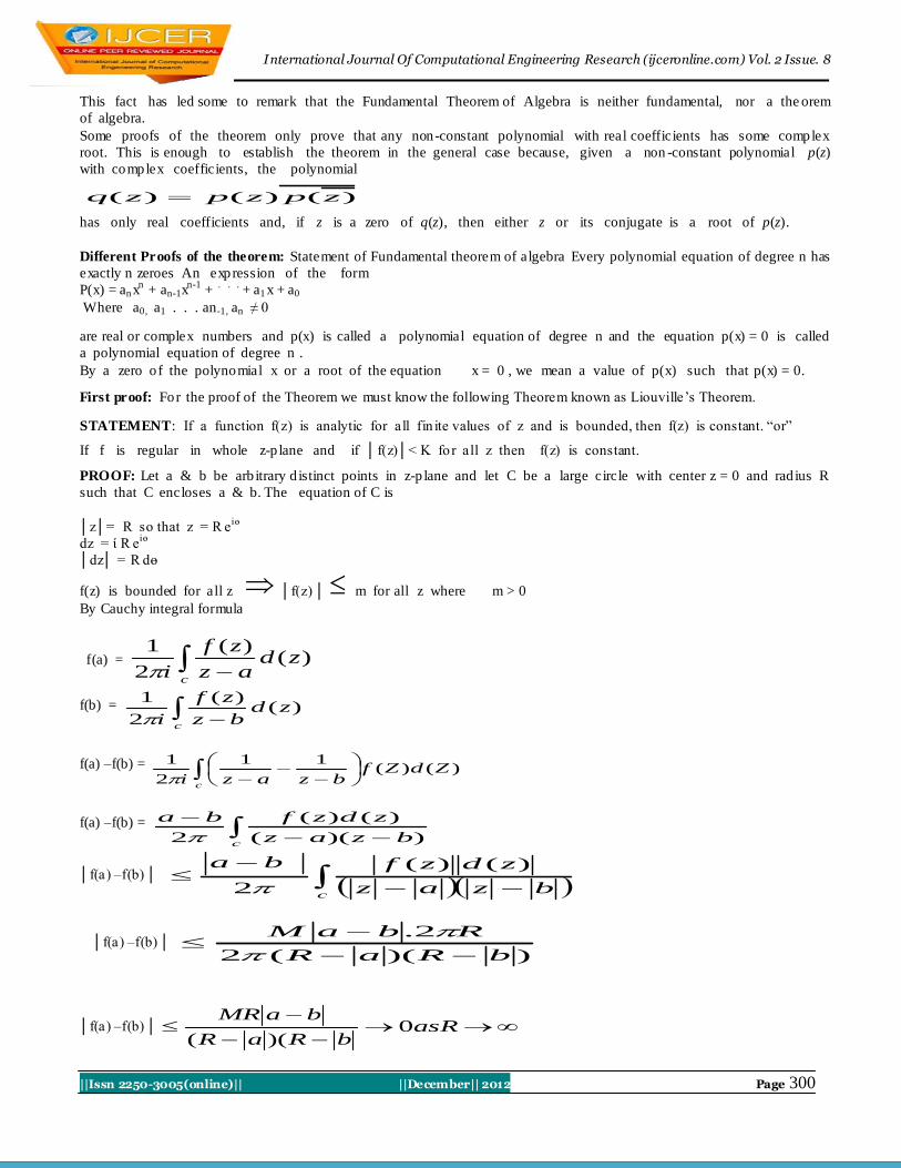
First proof: For the proof of the Theorem we must know the following Theorem known as Liouville‟s Theorem.

STATEMENT: If a function f(z) is analytic for all fin ite values of z and is bounded, then f(z) is constant. “or”

If f is regular in whole z-p lane and if │f(z)│< K fo r all z then f(z) is constant.

PROOF: Let a & b be arb itrary d istinct points in z-p lane and let C be a large circle with center z = 0 and rad ius R

such that C encloses a & b. The equation of C is

│z│= R so that z = R eiө

dz = ί R eiө

│dz│ = R dө

f(z) is bounded for all z │f(z) │ m for all z where m > 0

By Cauchy integral formula

f(a) = c

zdaz

zf

i)(

)(

2

1

f(b) = c

zdbz

zf

i)(

)(

2

1

f(a) –f(b) = )()(11

2

1ZdZf

bzazic

f(a) –f(b) =

cbzaz

zdzfba

))((

)()(

2

│f(a) –f(b) │

cbzaz

zdzfba )()(

2

│f(a) –f(b) │ ))((2

2.

bRaR

RbaM

│f(a) –f(b) │

asR

bRaR

baMR0

)((

International Journal Of Computational Engineering Research (ijceronline.com) Vol. 2 Issue. 8

||Issn 2250-3005(online)|| ||December|| 2012 Page 301

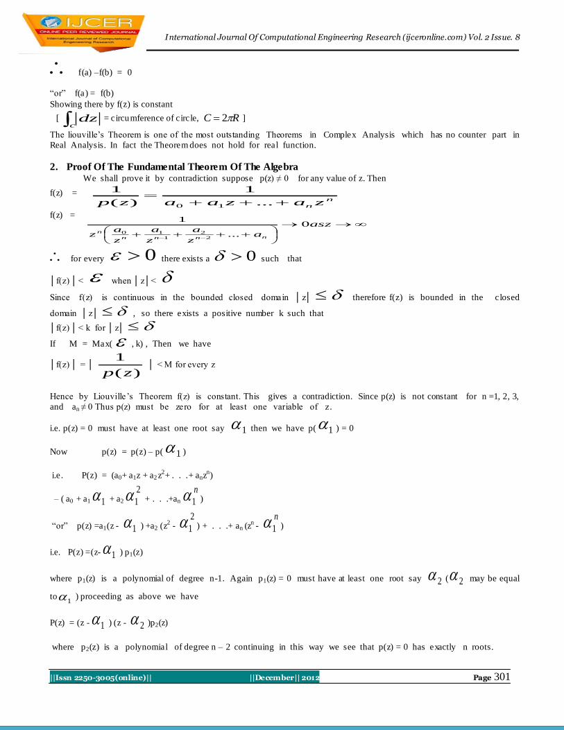
f(a) –f(b) = 0

“or” f(a) = f(b)

Showing there by f(z) is constant

[ c dz = circumference of circle, RC 2 ]

The liouville‟s Theorem is one of the most outstanding Theorems in Complex Analysis which has no counter part in

Real Analysis. In fact the Theorem does not hold for real function.

2. Proof Of The Fundamental Theorem Of The Algebra We shall prove it by contradiction suppose p(z) ≠ 0 for any value of z. Then

f(z) = n

n zazaazp

...

1

)(

1

10

f(z) =

asz

az

a

z

a

z

az nnnn

n

0

...

1

2

2

1

10

for every 0 there exists a 0 such that

│f(z) │< when │z│<

Since f(z) is continuous in the bounded closed domain │z│ therefore f(z) is bounded in the closed

domain │z│ , so there exists a positive number k such that

│f(z) │< k for │z│

If M = Max( , k) , Then we have

│f(z) │ = │)(

1

zp │ < M for every z

Hence by Liouville‟s Theorem f(z) is constant. This gives a contradiction. Since p(z) is not constant for n =1, 2, 3,

and an ≠ 0 Thus p(z) must be zero for at least one variable of z .

i.e. p(z) = 0 must have at least one root say 1 then we have p( 1 ) = 0

Now p(z) = p(z) – p( 1 )

i.e . P(z) = (a0+ a1z + a2 z2+ . . .+ anz

n)

– ( a0 + a1 1 + a2

2

1 + . . .+an

n

1 )

“or” p(z) =a1(z - 1 ) +a2 (z2 -

2

1 ) + . . .+ an (zn

- n

1 )

i.e. P(z) =(z- 1 ) p1(z)

where p1(z) is a polynomial of degree n-1. Again p1(z) = 0 must have at least one root say 2 ( 2 may be equal

to1 ) proceeding as above we have

P(z) = (z - 1 ) (z - 2 )p2(z)

where p2(z) is a polynomial of degree n – 2 continuing in this way we see that p(z) = 0 has exactly n roots.

International Journal Of Computational Engineering Research (ijceronline.com) Vol. 2 Issue. 8

||Issn 2250-3005(online)|| ||December|| 2012 Page 302

Second proof : For the second proof of the theorem we must know the following theorem known as Rouche‟s Theorem

Statement: If f(z) and g(z) are analytic inside and on a simple closed curve C and│g(z) │< │f(z) │ on C ,

Then f(z) and f(z) + g(z) both have the same number of zeros inside C

Proof : Suppose f(z) and g(z) are analytic inside and on a simple closed curve C and

│g(z) │< │f(z) │ on C

Firstly we shall prove that neither f(z) nor f(z) + g (z) has zero on C

If f(z) has a zero at z = a on C then f(a) = 0

But │g(z) │<│f(z) │on C

which is absurd Again if f(z) +g(z) has a zero at z = a on C

Then f(a) + g(a) = 0 so that

f(a) = - g(a)

“or”

│g(a) │ = │f(a) │

Again we get a contradiction , Thus neither f(z) nor f(z) + g(z) has a zero on C

Let N1 and N2 be number of the zeros of f and f + g respectively inside C.

we know that f and f + g both are analytic within and on C and have no poles inside C .

Therefore, by usual formula.

PNdzf

f

i c

'

2

1

gives 1

'

2

1Ndz

f

f

ic

and

2

''

2

1Ndz

gf

gf

ic

subtracting we get

12

'''

2

1NNdz

f

f

gf

gf

ic

(I)

Taking f

g so that g = f

│g│ < │f│ │

f

g│ < 1 │ │ < 1

Also gf

gf

''

= ff

fff

'''

= )1(

'1'

f

ff

“or”

1

''''

f

f

gf

gf

International Journal Of Computational Engineering Research (ijceronline.com) Vol. 2 Issue. 8

||Issn 2250-3005(online)|| ||December|| 2012 Page 303

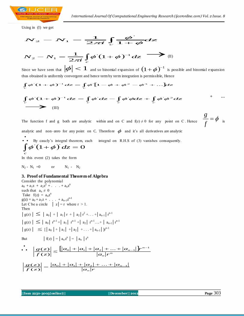
Using in (I) we get

dzi

NNc

12

1 '

12

dzi

NNc

1'

12 12

1

(II)

Since we have seen that 1 and so binomial expansion of 11

is possible and binomial expansion

thus obtained is uniformly convergent and hence term by term integration is permissible, Hence

dzdz

cc

...11 32'1'

dzdzdzdzcccc

2'''1' 1 + …

(III)

The function f and g both are analytic within and on C and f(z) ≠ 0 for any point on C . Hence

f

g is

analytic and non–zero for any point on C. Therefore and it‟s all derivatives are analytic

By caucly‟s integral theorem, each integral on R.H.S of (3) vanishes consequently.

01'' dz

c

In this event (2) takes the form

N2 - N1 =0 or N1 - N2

3. Proof of Fundamental Theorem of Algebra Consider the polynomial

a0 + a1z + a2z2

+ . . . + anzn

such that an ≠ 0

Take f(z) = anzn

g(z) = a0 + a1z + . . . + an-1zn-1

Let C be a circle │ z│= r where r > 1.

Then

│g(z) │ │ a0│ + │ a1│r + │ a2│r2 +. . . +│an-1│r

n-1

│g(z) │ │ a0│ rn-1

+│ a1│ rn-1

+│ a2│ rn-1

….+ │ an-1│rn-1

│g(z) │ [│a0 │+ │a1│ +│a2│ + . . . +│an-1│]rn-1

But │f(z) │= │an zn │= │an │r

n

n

n

n

n

ra

raaaa

zf

zg1

1210 ...

)(

)(

ra

aaaa

zf

zg

n

n 1210 ...

)(

)(

International Journal Of Computational Engineering Research (ijceronline.com) Vol. 2 Issue. 8

||Issn 2250-3005(online)|| ||December|| 2012 Page 304

Now if │g(z) │<│f(z) │ so that 1)(

)(

zf

zg , then

1... 1210

ra

aaaa

n

n

This

n

n

a

aaaar

1210 ...

Since r is arbitrary and hence by choosing r large enough, the last condition can be satisfied so th at │g(z)

│<│f(z)│. Now applying Rouche‟s theorem, we find that the given polynomial f(z) + g(z) has the same numbers

of zeros as f(z) But f(z) = anzn has exactly n zeros all located at z = 0 . Consequently f(z) +g(z) has exactly

n zeros. Consequently the given Polynomial has already n zeros.

Third Proof :For the proof we must know the fo llowing theorem known as Maximum Modulus princip le .

Statement:Suppose f(z) is analytic within and on a simple closed countor C and f(z) is not constant . Then │f(z) │ reaches its

maximum value on C (and not inside C), that is to say , if M is the maximum value of │f(z) │ on C, then │f(z) │ < M fo r

every z inside C.

PROOF: We prove this theorem by the method of contradiction, Analyicity of f(z) declares that f(z) is continuous within and

on C. Consequently │f(z)│ attains its maximum value M at the same point within or on C. we want to show that │f(z) │

attains the value M at a point lying on the boundary of C (and not inside C) . Suppose, if possible, this value is not attained on

the boundary of C but is attained at a point z = a within C so that

max│f(z) │=│f(a) │ = M……………(1)

and │f(z) │ ≤ M Z with in C………...(2)

Describe a circle Γ with a as center ly ing within C. Now f(z) is not constant and its continuity implies the existence of a point z

= b inside Γ such that │f(b) │ < M

Let > 0 be such that │f (b) │ = M -

Again │f(z) │ is continous at z = b

and so │[│f(z) │- │f(b) │]│ < 2

Whenever │z – b │ <

Since

│[│f(z) │- │f(b) │]│≥ │f(z) │- │f(b) │

“or” │f(z) │- │f(b) │ ≤ │[│f(z) │- │f(b) │]│< 2

“or” │f(z) │- │f(b) │< 2

“or” │f(z) │< │f(b) │+ 2

= M - +2

= M -

2

“or” │f(z) │< M - 2

z s.t │z – b │< …(3)

International Journal Of Computational Engineering Research (ijceronline.com) Vol. 2 Issue. 8

||Issn 2250-3005(online)|| ||December|| 2012 Page 305

We draw a circle γ with center at b and radius δ. Then (3) shows that

│f (z) │< M - 2

Z inside γ …………(4)

Again we draw another circle Ѓ with center at a and rad ius │b – a │= r

By Cauchy‟s Integral formula .

dzaz

zf

i

)(

2

1 f(a)

on Ѓ, z – a = reiө

i

ii

rie

driereaf

iaf

2

0

)(2

1)(

If we measure in anti-clock wise direction & if

< QPR = then

dreafaf i )(2

1)(

0

2

2

0

)(2

1)(

2

1)( dreafdreafaf ii

.

2

02

1

22

1)( MddMaf

42

2

22)(

MMMaf

Then M = │f (a) │ < M -

4

“or” M < M -

4

. A contradiction

For M cannot be less than M -

4

Hence the Required results follow.

International Journal Of Computational Engineering Research (ijceronline.com) Vol. 2 Issue. 8

||Issn 2250-3005(online)|| ||December|| 2012 Page 306

4. Minimum Modulus Principle STATEMENT:- Suppose f(z) is analytic within and on a closed contour C and Let f(z) ≠ 0 inside C suppose further that f(z)

is not constant . Then │f(z) │ attains its minimum value at a point on the boundary of “C” that is to say, if M is the

minimum value of │f(z) │ inside and on C. Then │f(z) │> m z inside C

PROOF:f(z) is analytic within and on C and f(z) ≠ 0 inside C. It follows that )(

1

zfis analytic within C. By Maximum

Modulus principal

)(

1

zf

attains its Maximum value on the boundary of C. So that │ )(zf │ attains its Minimum

value on the boundary of C. Hence the theorem

5. Proof Of The Fundamental Theorem Via Maximum

Modulus Principle Proof: Assume p(z) is non-constant and never zero. M such that |p(z)| |a0| ≠ 0 if |z| > M. Since |p

(z)| is continuous, it achieves its min imum on a closed interval. Let z0 be the value in the circle of radius M where p (z) takes

its minimum value.

So |p(z0)| |p(z)| for all z C, and in part icular

|p(z0)| |p(0)| = |a0|.

Translate the polynomial.

Let p (z) = p((z - z0) + z0);

Let p (z) = Q(z - z0).

Note the min imum of Q occurs at

z = 0: |Q(0)| |Q(z)| for all z C.

Q(z) = c0 + cj zj + · · · + cn z

n,

Where j is such that cj is the first coefficient (after c0) that is

Non-zero. I must show Q(0) = 0 Note if c0 = 0, we are done.

We may rewrite such that

Q(z) = c0 + cjzj + z

j+1 R(z)

We will ext ract roots.

Let

reiө

= -

jc

c0

Further, Let

j

i

j erz

1

1

So, 0czc j

j

Let 0 be a small real number. Then

)()(

)()(

1

1

1

1

01

1

1

1

1

101

zRzzcczQ

zRzzcczQ

jjj

j

j

j

jjjj

j

,1

1

1

00 Nzccjjj

Where N chosen such that )( 1zRN , and is chosen so that

International Journal Of Computational Engineering Research (ijceronline.com) Vol. 2 Issue. 8

||Issn 2250-3005(online)|| ||December|| 2012 Page 307

0

1

1

1 cz jjj

Thus,

,)( 01 czQ

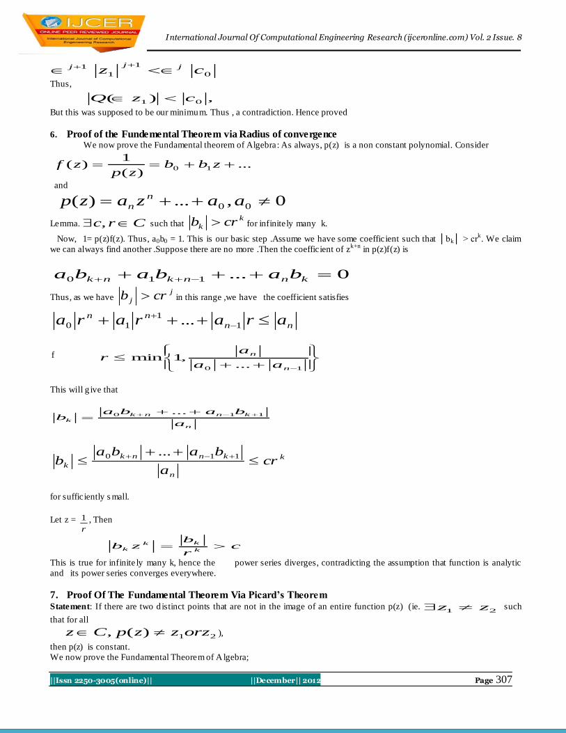
But this was supposed to be our minimum. Thus , a contradiction. Hence proved

6. Proof of the Fundemental Theorem via Radius of convergence

We now prove the Fundamental theorem of Algebra: As always, p(z) is a non constant polynomial. Consider

...)(

1)( 10 zbb

zpzf

and

0,...)( 00 aazazp n

n

Lemma. Crc , such that k

k crb for infinitely many k.

Now, 1= p(z)f(z). Thus, a0b0 = 1. This is our basic step .Assume we have some coefficient such that │bk│ > crk. We claim

we can always find another .Suppose there are no more .Then the coefficient of zk+n

in p(z)f(z) is

0...110 knnknk bababa

Thus, as we have j

j crb in this range ,we have the coefficient satisfies

nn

nn ararara

1

1

10 ...

f

10 ...,1min

n

n

aa

ar

This will g ive that

n

knnk

ka

babab

110 ...

k

n

knnk

k cra

babab

110 ...

for sufficiently s mall.

Let z = r

1 , Then

cr

bzb

k

kk

k

This is true for infinite ly many k, hence the power series diverges, contradicting the assumption that function is analytic

and its power series converges everywhere.

7. Proof Of The Fundamental Theorem Via Picard’s Theorem Statement: If there are two d istinct points that are not in the image of an entire function p(z) (ie.

21 zz such

that for all

21)(, orzzzpCz ),

then p(z) is constant.

We now prove the Fundamental Theorem of A lgebra;

International Journal Of Computational Engineering Research (ijceronline.com) Vol. 2 Issue. 8

||Issn 2250-3005(online)|| ||December|| 2012 Page 308

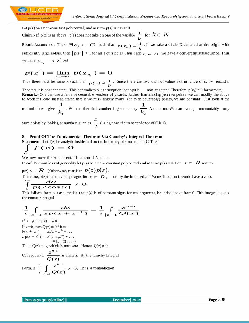
Let p(z) be a non-constant polynomial, and assume p(z) is never 0.

Claim:- If p(z) is as above , p(z) does not take on one of the variable k

1 fo r Nk

Proof: Assume not. Thus, Czk such that k

zp k

1)( . If we take a circle D centered at the orig in with

sufficiently large radius, then │p(z) │ > 1 for all z outside D. Thus each Dz 1, we have a convergent subsequence. Thus

we have 'zzin .but

0)(lim)( ' i

i

nn

zpzp .

Thus there must be some k such that k

zp1

)( . Since there are two distinct values not in range of p, by picard‟s

Theorem it is now constant. This contradicts our assumption that p(z) is non-constant. Therefore, p(z0) = 0 for some z0 .

Remark:- One can use a finite or countable versions of picards. Rather than missing just two points, we can modify the above

to work if Picard instead stated that if we miss finitely many (or even countably) points, we are constant. Just look at the

method above, gives

1

1

k. We can then find another larger one, say

2

1

k.And so on. We can even get uncountably many

such points by looking at numbers such as 2

(using now the transcendence of C is 1).

8. Proof Of The Fundamental Theorem Via Cauchy’s Integral Theorem Statement:- Let f(z) be analytic inside and on the boundary of some region C. Then

c

zf 0)(

We now prove the Fundamental Theorem of A lgebra.

Proof: Without loss of generality let p(z) be a non- constant polynomial and assume p(z) = 0. For Rz .assume

p(z) R (Otherwise, consider zpzp )( .

Therefore, p(z) doesn‟t change signs for Rz , or by the Intermediate Value Theorem it would have a zero.

2

0

0)cos2(p

d

This follows from our assumption that p(z) is of constant signs for real argument, bounded above from 0. This integral equals

the contour integral

1

1

1

1 )(

1

)(

1

z

n

zzQ

z

izzzp

dz

i

If z ≠ 0, Q(z) ≠ 0

If z =0, then Q(z) ≠ 0 Since

P(z + z-1

) = an(z + z-1

)+ . . .

znp(z + z

-1) = z

n(…anz

-n) + . . .

= an + z( . . . )

Thus, Q(z) = an, which is non-zero . Hence, Q(z) ≠ 0 ,

Consequently )(

1

zQ

z n

is analytic. By the Cauchy Integral

Formula

1

1

.0)(

1

z

n

zQ

z

i Thus, a contradiction!

International Journal Of Computational Engineering Research (ijceronline.com) Vol. 2 Issue. 8

||Issn 2250-3005(online)|| ||December|| 2012 Page 309

9. The Fundamental Theorem Of Algebra Our object is to prove that every non constant polynomial f(z) in one variable z ov er the complex numbers C

has a root, i.e. that is a complex number r in C such that f(r) = 0. Suppose that

f(z) = anzn + an-1z

n-1 + . . . + a1z + a0

where n is at least 1, an ≠ 0 and the coefficients ai are fixed complex numbers. The idea of the proof is as follows: we first

show that as |z| approaches infinity, |f(z)| approaches infinity as well. Since |f(z)| is a continuous function of z, it follows

that it has an absolute minimum. We shall prove that this minimum must be zero, which establishes the theorem. Complex

polynomial at a point where it does not vanish to decrease by moving along a line segment in a suitably chosen direction.

We first review some relevant facts from calcu lus.

10. Properties Of Real Numbers And Continuous Functions Lemma 1. Every sequence of real numbers has a monotone (nondecreasing or nonincreasing) subsequence. Proof. If

the sequence has some term which occurs infinitely many times this is clear. Otherwise, we may choose a subsequence in

which all the terms are distinct and work with that. Hence, assume that all terms are d istinct. Call an element "good" if it is

bigger than all the terms that follow it. If there are infinitely many good terms we are done: they will form a decreasing

subsequence. If there are only finitely many pick any term beyond the last of them. It is not good, so pick a term after it

that is bigger. That is not good, so pick a term after it that is bigger. Continuing in this way (officially, by mathemat ical

induction) we get a strict ly increasing subsequence. That proves the theorem

lemma 2. A bounded monotone sequence of real numbers converges.

Proof. Th is is sometimes taken as an axiom about the reals . What is given here is an intuitive justification. We assume the

sequence is non-decreasing: for the other case, take the negatives. The boundedness forces the integer parts of the terms in the

sequence to stabilize, since a bounded montone sequence of integers is eventually constant. Thus, eventually, the terms have

the form m + fn where m is a fixed integer, 0 is less than or equal to fn < 1, and the fn are non decreasing. The first digits

of the fn (after the decimal point) don't decrease and eventually stabilize: call the stable value a1. For the fn which begin with

.a1 ... the second digits increase and eventually stabilize: call the stable value a2. Continuing in this fashion we construct a

number f = .a1 a2 ... ah ... with the property that eventually all the fn agree with it to as many decimal p laces as we

like. It follows that fn approaches f as n approaches infinity, and that the original sequence converges to m + f. That proves

the theorem

Lemma 3. A bounded sequence of real numbers has a convergent subsequence. If the sequence is in the closed interval

[a,b], so is the limit.

Proof. Using Fact 1, it has a monotone subsequence, and this is also bounded. By Fact 2, the monotone subsequence

converges. It is easy to check that if all terms are at most b (respectively, at least a) then so is the limit. That proves the

theorem

Lemma 4. A sequence of points inside a closed rectangle (say a is less than or equal to x is less than or equal to b, c is less

than or equal to y is less than or equal to d) has a convergent subsequence. The limit is also in the rectangle.

Proof. Using Fact 3 we can pick out a subsequence such that the x-coordinates converge to apoint in [a,b]. Applying lemma 3

again, from this subsequence we can pick out a further subsequence such that the y-coordinates converge to a point in [c,d].

The x-coordinates of the points in this last subsequence still converge to a point in [a,b]. That proves the theorem

Lemma 5. A continuous real-valued function f defined on a closed rectangle in the plane is bounded and takes on an absolute

minimum and an absolute maximum value.

Proof. We prove the result for the maximum: for the other case consider -f. For each integer n = 1, 2, 3, ... divide the

rectangle into n2 congruent sub rectangles by drawing n-1 equally spaced vertical lines and the same number of equally

spaced horizontal lines. Choose a point in each of these sub rectangles (call these the special points at step n ) and evaluate f

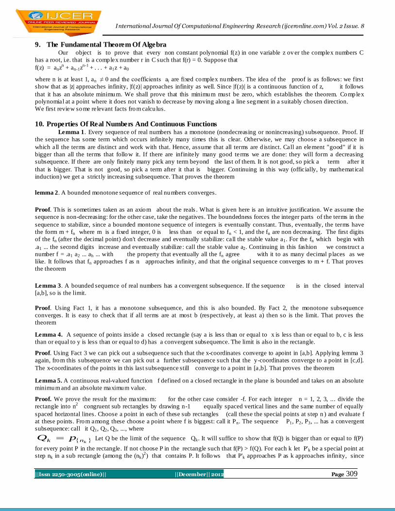
at these points. From among these choose a point where f is biggest: call it Pn. The sequence P1, P2, P3, ... has a convergent

subsequence: call it Q1, Q2, Q3, ..., where

knk pQ Let Q be the limit of the sequence Qk. It will suffice to show that f(Q) is bigger than or equal to f(P)

for every point P in the rectangle. If not choose P in the rectangle such that f(P) > f(Q). For each k let P'k be a special point at

step nk in a sub rectangle (among the (nk)2) that contains P. It follows that P'k approaches P as k approaches infinity, since

International Journal Of Computational Engineering Research (ijceronline.com) Vol. 2 Issue. 8

||Issn 2250-3005(online)|| ||December|| 2012 Page 310

both sides of the sub rectangles approach zero as k approaches infinity. For every k, f(Qk) is at least f(P'k), by the choice of

Qk. Taking the limit as k approaches infinity gives a contradiction, since f(Qk) approaches f(Q) and, by the continuity of f,

f(P'k) approaches f(P) as k approaches infinity. That proves the theorem. The result is valid for a continuous real- valued

function on any closed bounded set in R2 or R

n, where a set is closed if whenever a sequence of points in the set converges,

the limit point is in the set.

Lemma 6. Let f be a continuous real- valued function on the plane such that f(x,y) approaches infinity as (x,y) approaches

infinity. (This means that given any real number B, no matter how large, there is a real number m > 0 such that if x2 + y

2 is at

least m then f(x,y) is at least B.) Then f takes on an absolute min imum value at a point in the plane.}

Proof. Let B = f(0,0). Choose m > 0 such that if x2 + y

2 is at least m then f(x,y ) is at least B. Choose a rectangle that

contains the circle of radius m centered at the origin. Pick Q in the rectangle so that the minimum value of f on the

rectangle occurs at Q. Since (0,0) is in the rectangle f(Q) is at most B. Since outside the rectangle all values of f are at least B,

the value of f at Q is a minimum fo r the whole plane, not just the rectangle. That proves the theorem

Lemma 7. Let g be a continuous function of one real variable which takes on the values c and d on a certain interval. Then g

takes on every value r between c and d on that interval. Proof. Let g(a) = c and g(b) = d. We may assume without loss of

generality that a < b. Replacing g by g - r we may assume that g is positive at one endpoint, negative at the other, and never

vanishes. We shall get a contradiction. We shall construct a sequence of intervals I1 = [a,b], I2, ..., In, ... such that I[n+1] is

contained in In for each n, g has values of opposite sign at the end points of every In, and In has length 12

n

ab . In fact if I =

[an,bn] has already been constructed and M is the midpoint of In, then g (M) has opposite sign from at least one of

the numbers g(an), g(bn), and so we can choose one of [an, M] or [M, bn] for 1nI . The an are non decreasing, the bn

are non increasing, and an< bn for all n. It follows that both sequences have limits. But bn – an approaches 0 as n approaches

infinity, so the two limits are the same. Call the limit h. Since an approaches h, g(an) approaches g(h). Similarly, g(bn)

approaches g(h). Since g(an) and g(bn) have opposite signs for all n, this can only happen if g(h) = 0. That proves the

theorem

Remark:- Consider a polynomial f(x) with real coefficients of odd degree. Then lemma 7 implies that f has at least

one real root. To see this, we may assume that f has a posit ive leading coefficient (otherwise, replace f by -f). It is then

easy to see that f(x) approaches +infinity as x approaches + infinity while f(x) approaches -infinity as x approaches -

infinity. Since f(x) takes on both positive and negative values, lemma 7 implies that f takes on the value zero.

We want to note that if u, u' are complex numbers then

|u + u'| |u | + |u'|.

To see this note that, since both sides are non-negative, it suffices to prove this after squaring both sides, i.e. to show

that |u + u'|2 |u|

2 + 2|uu'| +|u'|

2. Now, it is easy to see that for any complex number v,

)(2

vvv ,

v where denotes the complex conjugate of v. Using this the inequality above is equivalent to

'''',' 2)( uuuuuuuuuu .

Multiply ing out, and canceling the terms which occur on both sides, yields the equivalen t inequality ''''' 2222 uuuuuuuuuuuu

Let w = u(u')-. Then '' uuuuw .

Thus, what we want to show is that www 2 .

If w = a + bi where a, b are real this becomes the assertion that 2a ≤ 2 {a2+b

2}

1/2

or a 22 ba ,

which is clear. Moreover, equality holds if and only if a is non negative and b is zero, i.e ., if and only

if )( 'uuw is a non-negative real number.

International Journal Of Computational Engineering Research (ijceronline.com) Vol. 2 Issue. 8

||Issn 2250-3005(online)|| ||December|| 2012 Page 311

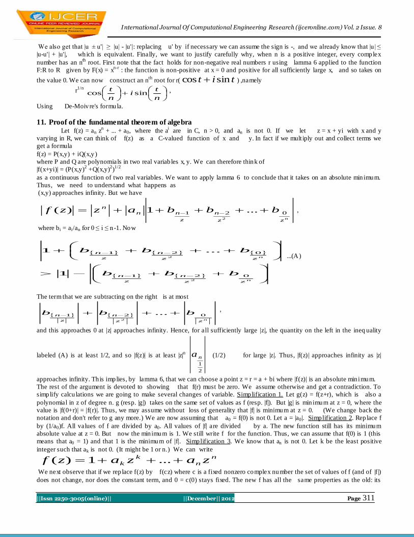
We also get that |u ± u'| ≥ |u| - |u'|: replacing u' by if necessary we can assume the sign is -, and we already know that |u | ≤

|u-u'| + |u'|, which is equivalent. Finally, we want to justify carefully why, when n is a positive integer, every complex

number has an nth

root. First note that the fact holds for non-negative real numbers r using lamma 6 applied to the function

F:R to R given by F(x) = xn-r

: the function is non-positive at x = 0 and positive for all sufficiently large x, and so takes on

the value 0. We can now construct an nth

root for r( tit sincos ) ,namely

r1/n

n

ti

n

tsincos ,

Using De-Moivre's formula.

11. Proof of the fundamental theorem of algebra Let f(z) = an z

n + ... + a0, where the a

i are in C, n > 0, and an is not 0. If we let z = x + yi with x and y

varying in R, we can think of f(z) as a C-valued function of x and y. In fact if we mult iply out and collect terms we

get a formula

f(z) = P(x,y) + iQ(x,y)

where P and Q are polynomials in two real variab les x, y. We can therefore think of

|f(x+yi)| = (P(x,y)2 +Q(x,y)

2)1/2

as a continuous function of two real variables. We want to apply lamma 6 to conclude that it takes on an absolute min imum.

Thus, we need to understand what happens as

(x,y) approaches infinity. But we have

nzz

n

z

nn

n bbbazzf 021 ...1)(2

,

where bi = ai/an for 0 ≤ i ≤ n -1. Now

n

n

zz

n

z

n

zz

n

z

n

bbb

bbb

021

021

2

2

1

...1...(A)

The term that we are subtracting on the right is at most

nzz

n

z

n bbb 021 ...2

,

and this approaches 0 at |z| approaches infinity. Hence, for all sufficiently large |z|, the quantity on the left in the ineq uality

labeled (A) is at least 1/2, and so |f(z)| is at least |z|n

2

1

na (1/2) for large |z|. Thus, |f(z) | approaches infinity as |z|

approaches infinity. Th is implies, by lamma 6, that we can choose a point z = r = a + bi where |f(z)| is an absolute min imum.

The rest of the argument is devoted to showing that f(r) must be zero. We assume otherwise and get a contradiction. To

simplify calcu lations we are going to make several changes of variable. Simplification 1. Let g(z) = f(z+r), which is also a

polynomial in z of degree n. g (resp. |g|) takes on the same set of values as f (resp. |f|). But |g| is min imum at z = 0, where the

value is |f(0+r)| = |f(r)|. Thus, we may assume without loss of generality that |f| is minimum at z = 0. (We change back the

notation and don't refer to g any more.) We are now assuming that a0 = f(0) is not 0. Let a = |a0|. Simplification 2. Rep lace f

by (1/a0)f. All values of f are divided by a0. All values of |f| are divided by a. The new function still has its minimum

absolute value at z = 0. But now the min imum is 1. We still write f for the function. Thus, we can assume that f(0) is 1 (this

means that a0 = 1) and that 1 is the minimum of |f|. Simplification 3. We know that an is not 0. Let k be the least positive

integer such that ak is not 0. (It might be 1 or n.) We can write n

n

k

k zazazf ...1)(

We next observe that if we rep lace f(z) by f(cz) where c is a fixed nonzero complex number the set of values of f (and of |f|)

does not change, nor does the constant term, and 0 = c(0) stays fixed. The new f has all the same properties as the old: its

International Journal Of Computational Engineering Research (ijceronline.com) Vol. 2 Issue. 8

||Issn 2250-3005(online)|| ||December|| 2012 Page 312

absolute value is still min imum at z = 0. It makes life simplest if we choose c to be a kth

root of (-1/ak). The new f we get

when we substitute cz for z then turns out to be 1 – zk + a'k+1 z

k+1 + ... + a'n z

n. Thus, there is no loss of generality in

assuming that ak = -1. Therefore, we may assume that

f(z) = 1 – zk + ak+1 z

k+1+ ... +an z

n.

If n = k then f(z) = 1 – zn and we are done, since f(1) = 0. Assume from here on that k is less than n. The main point. We

are now ready to finish the proof. All we need to do is show with f(z) = 1 – zk + ak+1z

k+1 + ...+ anz

n that the minimum

absolute value of f is less than 1, contradicting the situation we have managed to set up by assuming that f(r) is not 0. We shall

show that the absolute value is indeed less than one when z is a s mall positive real number (as we move in the complex p la ne

away from the origin along the positive real axis or x-axis, the absolute value of f(z) drops from 1.) To see this assume that z

is a positive real number with 0 < z < 1. Note that 1-z is then positive. We can then write

|f(z)| =|1 – zk + ak+1z

k+1 + ... + anz

n |

≤ |1-zk|+|ak+1z

k+...+anz

n|

= 1- zk + | ak+1z

k+1 + ... + anz

n|

≤1- zk + | ak+1|z

k+1 + . . . + |an|z

n

(keep in mind that z is a positive real number)

= 1 - zk (1 – wz), where

wz = | ak+1|z + ... +|an|zn-k

.

When z approaches 0 through positive values so does wz. Hence, when z is a s mall positive real number, so is z (1-wz), and so

for z a s mall positive real number we have that

0 < 1 – zk(1-wz) < 1.

Since |f(z)| < 1 – zk(1-wz)

it follows that |f(z)| takes on values smaller than 1, and so |f(z)| is not min imum at z = 0 after all. Th is is a cont radiction. It

follows that the minimum value of |f(z)| must be 0, and so f has a root .That proves the theorem.

12. Fundemental Theorem of Algebra via Fermat’s Last Theorem For the proof of the theorem we must know the following lemmas

Lemma 1:If an algebraic equation f(x) has a root α, then f(x) can be divided by x-α without a remainder and the degree of the

result f'(x) is less than the degree of f(x).

Proof:

Let f(x) = xn

+ a1 xn-1

+ . . . + an-1x + an

Let α be a root such that f(α) = 0

Now, if we div ide the polynomial by (x-α), we get the following

f(x)/(x - α) = f1(x) + R/(x-α)

where R is a constant and f1(x) is a polynomial with order n -1.

Multiplying both sides with x-α gives us:

f(x) = (x - α)f1(x) + R

Now, if we substitute α for x we get:

f(α) = 0 which means that the constant in the equation is 0 so R = 0. That proves the lemma.

Theorem: Fundamental Theorem of Algebra

For any polynomial equation of order n, there exist n roots ri such that:

xn + a1 x n-1

+ ... + an-1 x + an = (x – r1)(x – r2) . . . (x – rn)

Proof: Let f(x) = xn + a1 xn-1

+ ... + an-1 x + an

We know that f(x) has at least one solution α1.

Using Lemma 1 above, we know that:

f(x)/(x – α1) = f'(x) where deg f'(x) = n-1.

International Journal Of Computational Engineering Research (ijceronline.com) Vol. 2 Issue. 8

||Issn 2250-3005(online)|| ||December|| 2012 Page 313

So that we have:

f(x) = (x – α1)f'(x)

But we know f'(x) has at least one solution α2

f'(x)/ (x–α2) = f''(x) where deg f''(x) = n-2. And

f(x) = (x – α1)(x – α2)f''(x)

Eventually we get to the point where the degree of

fn(x)=1 .In this case, fn(x) = x – αn. This establishes that there are n roots for a given equation f(x) where the

degree is n. Putting this all together gives us:

f(x) = (x – α1)(x – α2). . . (x – αn)

Now, since f(x)=0 only when one of the values α i=x, we see that the n roots αi are the only solutions.

So, we have proven that each equation is equal to n roots.One important point to remember is that the n roots are not

necessarily distinct. That is, it is possible that α i = αj where i ≠ j. That proves the theorem

Fundamental theorem of A lgebra due to Cauchy

We will prove

f(z) = zn

+ a1zn-1

+ a2zn-1

+ . . . + an = 0

where ai are complex numbers n ≥ 1 has a complex root.

Proof:- let an ≠ 0 denote z = x + iy x, y real Then the function

g(x ,y) = │f(z) │= │f(x + iy) │

Is defined and continuous in R2

Let

n

j

jac1

it is +ve using the triangle inequality

We make the estimation

n

nn

z

a

z

a

z

azzf ...

21)(

2

1

n

n

z

a

z

a

z

azf ...1)(

21

nnz

z

czzf

2

11)(

Being true for cz 2,1max denote nnacr 2,2,1max: conside the

disk ryx 22 Because it is compact the function g(x,y) attains at a point (x0 y0) of the disk its absolute

minimum value (infimum) in the disk if │z│> r we have

022

1

2

1

2

1)(),( n

nn

nnaarzzfyxg

Thus

rzforzfagyxg n )()0,0(),(

Hence ),( 00 yxg is the absolute min imum of g(x,y) in the whole complex plane

we show that g(x0 y0) = 0 therefore we make the antitheses that g(x0y0) > 0

Denote UBziyxz 0000

nn

nn UUbUbbuzfzf

1

110 ...)()(

Then bn = f(z0) ≠ 0 by the antithesis

International Journal Of Computational Engineering Research (ijceronline.com) Vol. 2 Issue. 8

||Issn 2250-3005(online)|| ||December|| 2012 Page 314

More over denote

nn

j

jb

cnib

bc

1),...12( 0

And assume that cn-1 = cn-2 = . . . = cn-k+1 = 0

But cn-k ≠ 0 then we may write

)...1()( 0

1

1

kk

knknknn ucucuccbzf

If )sin(cos&)sin(cos

euipuc k

kn

Then

)sin()(cos kiknk

kn peuc

By Demorvie‟s identity choosing

k

&1 we get

kk

kn peuc & can make the estimate

11

01

0

1

10

1

1

Re...

......

kk

kn

nk

kn

nk

kn

ecc

ccecucuc

Where R is constant

Let now

k

R

p

p

i

2.,1min we obtain

uhpebzf k

n 1)(

1Re1)(

)(1)(

kk

n

k

n

pebzf

uhpebzf

)(2

21

0zfbnb

R

pRpeb

n

k

n

Which results is impossible since │f(z) │ was absolute minimum. Consequently the antithesis is wrong & the proof is settled.

13. Another Proof Of Fundamental Theorem Of Algebra The proof depends on the following four lemmas

Lemma1: Any odd-degree real polynomial must have a real root.

Proof:

We know from intermediate value theorem, suppose xRxp )( with degree p(x) = 2k +1 and

suppose the leading coefficient an > 0

( the proof is almost identical if an > 0). Then

International Journal Of Computational Engineering Research (ijceronline.com) Vol. 2 Issue. 8

||Issn 2250-3005(online)|| ||December|| 2012 Page 315

P(x) = an xn + (lower terms)

And n is odd . Then,

(1)

n

nxx xaxp lim)(lim since an > 0.

(2)

n

nxx xaxp lim)(lim

since an > 0 and n is odd.

From (1) , p(x) gets arbitrarily large positively , so there exists an x1 with p(x1) > 0 . Similarly, from (2) their exits an x2 with

p(x2) < 0 A real polynomial is a continuous real – valued function for all Rx , Since p(x1) p (x2) < 0, it fo llows by the

intermediate value theorem that their exits an x3 , between x1 and x2, such that p(x3 ) = 0.

Lemma 2: Any degree two complex polynomials must have a complex root.

Proof: We know from consequence of the quadratic formula and of the fact that any complex number has a square root.

If p(x) = ax2 + bx + c, a ≠ 0, then the roots formally are

a

acbbx

a

acbbx

2

4,

2

4 2

2

2

1

From DeMoivere‟s theorem every complex number has a square root, hence x1 , x2 exists in C. They of course may be same if

b2 - 4ac = 0.

Lemma 3: If every non-constant real polynomial has a complex root, then every non-constant complex polynomial has a

complex root.

Proof: According to concept of the conjugate of complex polynomial

Let xRxP )( and suppose that every non-constant real polynomial has at least one complex root. Let

).()()( xPxPxH from previous lemma xRxH )( . By supposition there exists a Cz 0 with

H(z0) = 0. then

0)()( 00 zPzP ,

And since C has no zero d ivisors, either

)( 0zP = 0 or )( 0zP = 0.

then previous lemmas

0)()()( 000 zPzPzP .

Therefore, 0z is root of p(x).

Lemma 4:-

Any non-constant real polynomial has a complex root.

Proof: Let xRxa. . .x a a f(x) n

n10

with n ≥ 1 , an ≠ 0. The proof is an induction on the degree n of f(x). Suppose n = 2mq where q is odd. We do the induction on

m. if m = 0 then f(x) has odd degree and the theorem is true from lemma 1. Assume then that theorem is true for all degrees d

= 2k q

‟ where k > m and q

‟ is odd . Now assume that the degree of f(x) is n = 2

mq. Suppose F

‟ is the splitting field for f(x) over

R in which the roots are n ,...,1 . We show that at least one of these roots must be in C. ( In fact, all are in C but to

prove the lemma we need only show at least one.)

Let Zh and from the polynomial

))(()( ji

ji

i hjxxH

International Journal Of Computational Engineering Research (ijceronline.com) Vol. 2 Issue. 8

||Issn 2250-3005(online)|| ||December|| 2012 Page 316

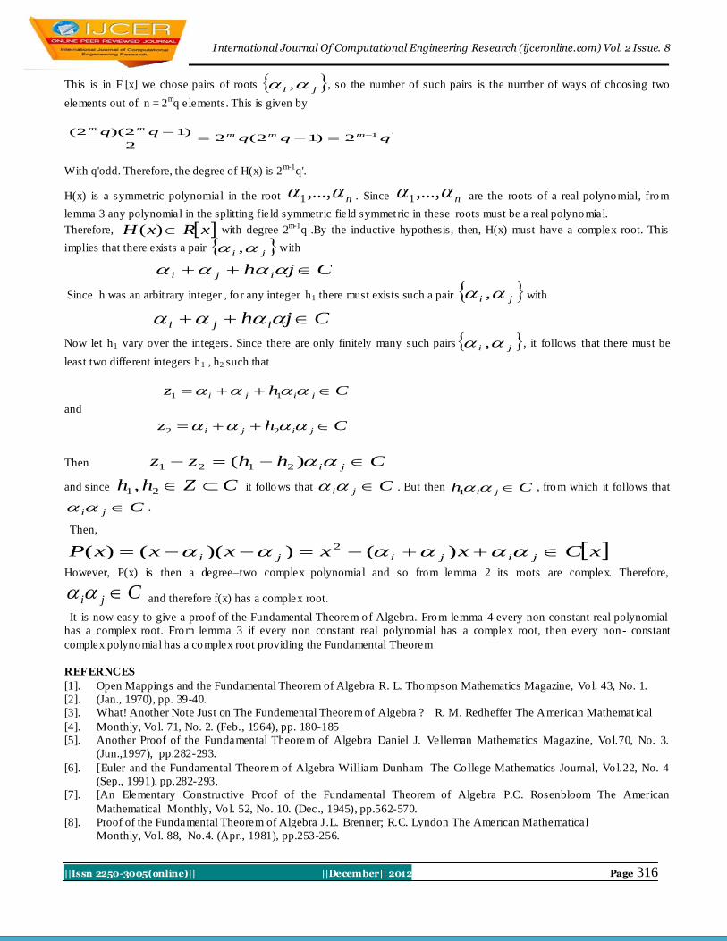
This is in F‟[x] we chose pairs of roots

ji , , so the number of such pairs is the number of ways of choosing two

elements out of n = 2mq elements. This is given by

'12)12(22

)12)(2(qqq

qq mmmmm

With q'odd. Therefore, the degree of H(x) is 2m-1

q'.

H(x) is a symmetric polynomial in the root n ,...,1 . Since n ,...,1 are the roots of a real polynomial, from

lemma 3 any polynomial in the splitting field symmetric field symmetric in these roots must be a real polynomial.

Therefore, xRxH )( with degree 2m-1

q‟.By the inductive hypothesis, then, H(x) must have a complex root. This

implies that there exists a pair ji , with

Cjh iji

Since h was an arbit rary integer , fo r any integer h1 there must exists such a pair ji , with

Cjh iji

Now let h1 vary over the integers. Since there are only finitely many such pairs ji , , it follows that there must be

least two different integers h1 , h2 such that

Chz jiji 11

and

Chz jiji 22

Then Chhzz ji )( 2121

and since CZhh 21, it follows that Cji . But then Ch ji 1 , from which it follows that

Cji .

Then,

xCxxxxxP jijiji )())(()( 2

However, P(x) is then a degree–two complex polynomial and so from lemma 2 its roots are complex. Therefore,

Cji and therefore f(x) has a complex root.

It is now easy to give a proof of the Fundamental Theorem of Algebra. From lemma 4 every non constant real polynomial

has a complex root. From lemma 3 if every non constant real polynomial has a complex root, then every non - constant

complex polynomial has a complex root providing the Fundamental Theorem

REFERNCES

[1]. Open Mappings and the Fundamental Theorem of Algebra R. L. Thompson Mathematics Magazine, Vol. 43, No. 1.

[2]. (Jan., 1970), pp. 39-40.

[3]. What! Another Note Just on The Fundemental Theorem of Algebra ? R. M. Redheffer The American Mathemat ical

[4]. Monthly, Vol. 71, No. 2. (Feb., 1964), pp. 180-185

[5]. Another Proof of the Fundamental Theorem of Algebra Daniel J. Velleman Mathematics Magazine, Vol.70, No. 3.

(Jun.,1997), pp.282-293.

[6]. [Euler and the Fundamental Theorem of Algebra William Dunham The College Mathematics Journal, Vol.22, No. 4

(Sep., 1991), pp.282-293.

[7]. [An Elementary Constructive Proof of the Fundamental Theorem of Algebra P.C. Rosenbloom The American

Mathematical Monthly, Vol. 52, No. 10. (Dec., 1945), pp.562-570.

[8]. Proof of the Fundamental Theorem of Algebra J.L. Brenner; R.C. Lyndon The American Mathematical

Monthly, Vol. 88, No.4. (Apr., 1981), pp.253-256.

International Journal Of Computational Engineering Research (ijceronline.com) Vol. 2 Issue. 8

||Issn 2250-3005(online)|| ||December|| 2012 Page 317

[9]. [Yet Another Proof of the Fundamental Theorem of Algebra R.P. Boas,Jr. The American Mathematical Monthly, Vol.

71, No. 2. (Feb., 1964), p.180.

[10]. The Fundamental Theorem of Algebra Raymond Redheffer The American Mathematical Monthly, Vol. 64,

[11]. No. 8 (Oct.,1957), pp.582-585.

[12]. A Proof of the Fundamental Theorem of Algebra R.P.Boas, Jr. The American Mathemat ical Monthly,

[13]. Vol. 42, No. 8.(Oct.,1935), pp.501-502

[14]. An Easy Proof of the Fundamental Theorem of Algebra Charles Fefferman The American Mathematical

[15]. Monthly, Vol. 74, No. 7. (Aug.- Sep., 1967), pp.854-855[11] Eu lers: The Masster of Us All William Dunham

[16]. The Mathematica Association of America Dolciani Mathematical Expositions No.22, 1999.

[17]. The Fundamental Theorem of Algebra Benjamin Fine Gerhard Rosenberger Springer New York

[18]. Mathematical Analysis S.C Malik, Savita Arora New Age International Publication

[19]. Functions of a Complex Variable Goyal & Gupta Pragati Prakajhan Publication

[20]. A.R. Schep, A Simple Complex Analysis and an Advanced Ca lculus Proof o f the FundamentalTheorem

[21]. of Algebra, Am Math Monthly 116, Jan 2009,67-67

[22]. David Antin‟s translation of Heinrich Dorrie‟s 100 Great Problems of Elementary

[23]. A. R. Schep, A Simple Complex Analysis and an Advanced Calculus Proof o f the Fundamental Theorem of

[24]. Algebra, Am Math Monthly 116, Jan 2009, 67-68.

[25]. Heinrich Dorrie, 100 Great Problems of Elementary Mathemat ics.

[26]. Complex Analysis Kunihiko Kodaira Cambridge Studies in advanced mathematics

[27]. Elementary Theory of Analytic Functions of one or Several Complex Variables Henri Cartan

[28]. Complex variables An introduction Carlos A. Berenstein Roger gar Springer-Verlag

[29]. Fundamental Theorems of Operator Algebra V.1 Elementary Theorem V.2 Advanced Theorem Kadison- Richard.

[30]. Fundamental Theorem of Algebra Fine and Gerhard

[31]. Fundamentals of College algebraic Miller

[32]. Fundamental concept of higher Algebra Albert.

[33]. Fundamental concept of Algebra Meserve.

[34]. Fundamental Concept of Algebra Chevalley. C

[35]. Fundemental Theorey of One Complex Variable Green and Krantz

[36]. Function of complex variab le Franklin

[37]. Function of Complex Variable with applicat ion Phillips vig Theory & Technique carrier range.

[38]. Function of a Complex variab le and some of their applicat ions Fuchs and Shabat Smitnov & Lebeder

[39]. Function of complex variab le Goursat E.

[40]. Function of complex variab le Conway J.B

[41]. Function of one complex variable Macrobart TM

[42]. Foundation of the Theorem of Algebras Volume I & Volume II Hankoock. Harris

[43]. Complex Analysis Freitag Busam

[44]. Function of Several variab les lang.