fundamental period prediction of steel plate shear wall
TRANSCRIPT

FUNDAMENTAL PERIOD PREDICTION OF STEEL PLATE SHEAR WALLSTRUCTURES
A Thesis submitted to the faculty of San Francisco State University
In partial fulfillment of The requirements for
The Degree
. V: 4-'2- Master of Science
In
Engineering: Structural/Earthquake Engineering
By
Benjamin Aaron Kean
San Francisco, California
May 2017

Copyright by Benjamin Aaron Kean
2017

CERTIFICATION OF APPROVAL
I certify that I have read Fundamental Period Prediction o f Steel Plate Shear Wall
Structures by Benjamin Aaron Kean, and that in my opinion this work meets the
criteria for approving a thesis submitted in partial fulfillment of the requirement for
the degree Master of Science in Engineering: Structural/Earthquake Engineering at
San Francisco State University.
Cheng Chen, Ph.D.Professor of Civil Engineering
Professor of Civil Engineering

Fundamental Period Prediction of Steel Plate Shear Wall Structures
Benjamin Aaron Kean San Francisco, California
2017
The Steel Plate Shear Wall (SPSW) is a structural system used today in design for
the primary Lateral Force Resisting System (LFRS) of a building. In the initial
design stage the fundamental period of the structure is used to calculate the seismic
forces using the Equivalent Lateral Force Procedure (ELFP). The American Society
of Civil Engineers (ASCE) allows for the approximation of the fundamental period
to be performed using a general formula using two coefficients whose values are
dependent on the type of LFRS. The SPSW uses a general value for the
fundamental period coefficients and it has been shown that the current procedure
for approximating the fundamental period of an SPSW produces overly
conservative estimations. This study evaluates the fundamental period of a large
population of SPSW prototypes. A formula for better approximation of the
fundamental period coefficients is derived and then verified on code-designed
SPSW prototypes.
I certify that the Abstract is a correct representation of the content of this thesis.
Date

PREFACE AND/OR ACKNOWLEDGEMENTS
I would like to thank the efforts of Dr. Cheng Chen, Amado Flores Renteria, Jolani
Chun-Moy, Daniel Salmeron, and David Flores for making this research possible.
Amado Flores Renteria, Jolani Chun-Moy, Daniel Salmeron, and David Flores
contributed as undergraduate students in the process of design and analysis of the
5-,8-, and 10-story SPSWs. Acknowledgements are also given to Ramin Bahargi
and Shihang Guo who contributed on the 3-, 6-, and 9-Story SPSWs. The author
would also like to acknowledge the constant support of his family and friends. The
results and findings in this thesis would not be possible without the help from the
individuals listed above.

TABLE OF CONTENTS
List of Table.................................................................................................................. viii
List of Figures...................................................................................................................x
List of Appendices.......................................................................................................... ix
CHAPTER 1. INTRODUCTION..................................................................................1
1.1 The Steel Plate Shear W all..........................................................................1
1.1.1 Previous SPSW research............................................................. 3
1.2 Current Code for Fundamental Period Estimation for SPSW ................. 5
1.3 Previous Research on Fundamental Period Estimation for S P S W 6
1.3.1 Liu etal. Approximation M ethod.............................................. 6
1.3.2 Topkaya and Kurban Approximation M ethod..........................8
CHAPTER 2. DESIGN OF SPSW PROTOTYPES.................................................10
2.1 Building Information..................................................................................10
2.2 Design of SPSW Prototypes......................................................................12
2.3 SPSW Prototype Design Summary...........................................................13
2.3.1 3-Story SPSW Design Summary..............................................13
2.3.2 5-Story SPSW Design Summary..............................................14
2.3.3 6-Story SPSW Design Summary..............................................15
2.3.4 8-Story SPSW Design Summary..............................................15
2.3.5 9-Story SPSW Design Summary..............................................16
2.3.6 10-Story SPSW Design Summary........................................... 17

CHAPTER 3. FUNDAMENTAL PERIOD APPROXIMATION METHODS ...19
3.1 Equivalent Lateral Force Procedure..........................................................19
3.1.1 Approximation of Fundamental Period.................................. 20
3.1.2 Seismic Response Coefficient...................................................24
3.2 Proposed Simplified Fundamental Period Approximation Methods...27
3.2.1 Liu etal. Approximation Method ........................................... 28
3.2.1.1 Application of Liu et al. method..............................30
3.2.2 Topkaya and Kurban Approximation M ethod....................... 32
3.2.2.1 Application of Topkaya and Kurbans method.......34
3.3 Comparison of Period Approximations...................................................37
CHAPTER 4. FINITE ELEMENT MODELING.....................................................44
4.1 Open System for Earthquake Engineering Simulation (OpenSees) ....44
4.2 Modeling of SPSW prototypes.................................................................44
4.3 Panel Zone Modeling.................................................................................46
CHAPTER 5. STATISTICAL ANALYSIS..............................................................50
5.1 Statistical Analysis of the SPSW Prototypes..........................................50
5.2 Bay-Width Adjustment..............................................................................52
5.2.1 Coefficient C t..............................................................................52
5.2.2 Coefficient x................................................................................ 54
5.3 Derivation of Base-Shear Participation Adjustment Function..............56
5.3.1 Ct Coefficient Adjustment........................................................ 57
5.3.2 x Coefficient Adjustment.......................................................... 61
5.3.3 Error Analysis.............................................................................66
5.4 Proposed Method for Approximating SPSW Fundamental Period.....67

CHAPTER 6. VALIDATION OF PROPOSED METHOD................................... 70
6.1 SPSW Validation Prototypes.................................................................... 70
6.2 Results from Approximation M ethod...................................................... 71
6.3 Summary......................................................................................................75
CHAPTER 7. CONCLUSIONS.................................................................................. 82
REFERENCES...............................................................................................................83
vii

LIST OF TABLES
Table 1-1. Values of Parameters Ct and x .................................................................... 6
Table 2-1. Seismic mass and weights for SPSW prototypes...................................10
Table 2-2. Design summary SPSW prototype 3M100.............................................14
Table 2-3. Design summary SPSW prototype 5M100............................................ 14
Table 2-4. Design summary SPSW 6M100................................................................ 15
Table 2-5. Design summary SPSW 8M100................................................................ 16
Table 2-6. Design summary SPSW 9M100................................................................ 17
Table 2-7. Design summary SPSW 10M100.............................................................. 18
Table 3-2. Values for factor r f ..................................................................................... 21
Table 3-3. 10-foot bay width fundamental period results.........................................33
Table 3-4. 15-foot bay width fundamental period results.........................................40
Table 3-5. 20-foot bay width fundamental period results.........................................41
Table 5-1. Fundamental period coefficients from regression analysis...................42
Table 5-2. /(L ) values for fundamental period coefficient fc(L ) ............................51
Table 5-3. Values for ^c100ari^ c 100 ............................................................................^3
Table 5-4. Coefficient values for the adjustment function.......................................55
Table 5-5. Coefficient values for the adjustment function/*(L)..............................55
Table 5-6. fac(V) at varying levels of base-shear participation..............................58
Table 5-7. fpc(V) at varying levels of base-shear participation............................. 58
Table 5-8. Values for aUc and bac assuming a power series model....................... 60
Table 5-9. Values for apc and bpc assuming a power series m odel...................... 60
Table 5-10. Values for aUc and bac assuming a linear variation.............................61
viii

Table 5-11. Values for a.pc and bpc assuming a linear variation.............................. 61
Table 5-12. Values of fax(Y) at varying base-shear participation levels...............62
Table 5-13. Values of fpx(V) values at each base-shear participation value 62
Table 5-14. Values for aUxand /^assum ing a power series variation.................65
Table 5-15. Values for a^x and bpx assuming a power series variation................65
Table 5-16. Values for aUx and bUx assuming a linear variation...........................65
Table 5-17. Values for a^x and bpx assuming a linear variation.............................66
Table 5-18. Root Mean Squared Analysis for the power series and linear model66
Table 5-19. Values of all coefficients used in proposed method............................68
Table 6-1. 3K100 SPSW design sum m ary.................................................................70
Table 6-2. 4N80 SPSW design summary................................................................... 71
Table 6-3. 7W60 SPSW Design Summary.................................................................71
Table 6-4. Comparison of fundamental periods from finite element analysis and the proposed method for the three validation prototypes.......................................... 74
Table 6-5. Proposed method coefficient values........................................................ 76
Table 6-6. 10-foot bay-width SPSW fundamental period results............................79
Table 6-7. 15-foot bay-width SPSW fundamental period results............................80
Table 6-8. 20-foot bay-width SPSW fundamental period results............................81

LIST OF FIGURES
Figure 1-1 Typical SPSW configuration [1],
Figure 1-2 Hour-glass shape of web-plate due to pull-in effect (courtesy of Carlos Ventura, University of Columbia, Vancouver, Canada) [1]....................................... 4
Figure 2-1. Floor plan for 3-story SPSW prototypes................................................. 11
Figure 2-2. Floor plan for 5-, 6-, 8-, 9-, and 10-story SPSW prototypes..................11
Figure 3-1. Comparison of fundamental period for SPSW prototypes designed with 100 percent base shear..........................................................................................22
Figure 3-2. Comparison of fundamental period for SPSW prototypes designed with 85 percent base shear.........................................................................................23
Figure 3-3. Comparison of fundamental period for SPSW prototypes designed with 65 percent base shear..........................................................................................24
Figure 3-4. Comparison of Cs max values of SPSW N prototypes........................26
Figure 3-5. Comparison of Cs max values of SPSW M prototypes........................26
Figure 3-6. Comparison of Cs max values o f SPSW W prototypes........................27
Figure 3-7. Application of Liu et al. method to 10-foot bay-width SPSW prototypes........................................................................................................................ 30
Figure 3-8. Application of Liu et al. method to 15-foot bay-width SPSW prototypes........................................................................................................................ 31
Figure 3-9. Application of Liu et al. method to 20-foot bay-width SPSW prototypes........................................................................................................................ 31
Figure 3-10. 10-foot bay width SPSW results from Topkayas SPSW fundamental period m ethod.................................................................................................................35
Figure 3-11. 15-foot bay width SPSW results from Topkayas SPSW fundamental period m ethod.................................................................................................................36
Figure 3-12. 20-foot bay width SPSW results from Topkayas SPSW fundamental period m ethod.................................................................................................................37
Figure 3-13. 10-foot SPSW period approximations from Liu and Topkaya..... 38
Figure 3-14. 15-foot SPSW period approximations from Liu and Topkaya.....38
Figure 3-15. 20-foot SPSW period approximations from Liu and Topkaya.....39
Figure 4-1. Visualization o f the strip method [1 ] ......................................................45
Figure 4-2. 6-Story OpenSees SPSW m odel............................................................ 46
Figure 4-3. Visualization of a typical panel zone configuration at beam-to-column connection....................................................................................................................... 47
Figure 4-4. HBE node conventions for typical SPSW web-plate............................48
Figure 4-5. Configuration of the modified panel zones............................................ 49
Figure 5-1. Comparison between periods from regression and finite element analysis.............................................................................................................................51
Figure 5-2. Comparison of adjusted Ct values and finite element values.............54
Figure 5-3. Validation o f power series assumption for “x” coefficient adjustment function............................................................................................................................56
Figure 5-4. aC over base-shear participation levels..................................................59
Figure 5-5. PC over base-shear participation levels..................................................59
Figure 5-6. Variation o f ax over base-shear participation levels.............................63
Figure 5-7. Variation of Px over base-shear participation levels.............................64
Figure 5-8. Results from application of proposed method on SPSW prototypes ..69
Figure 6-1. Comparing fundamental period analysis methods for the first validation SPSW prototype, SPSW 3K 100................................................................72
Figure 6-2. Comparing fundamental period analysis methods for the second validation SPSW prototype, SPSW 4N 80..................................................................73
Figure 6-3. Comparing fundamental period analysis methods for the third validation SPSW prototype, SPSW 7W60..................................................................74
Figure 6-4. 10-foot bay-width SPSW fundamental period results..........................77


LIST OF APPENDICES
A-2-1. 3-STORY SPSW DESIGN SUMMARIES.................................................... 87
A-2-2. 5-STORY SPSW DESIGN SUMMARIES.................................................... 88
A-2-3. 6-STORY SPSW DESIGN SUMMARIES....................................................89
A-2-4. 8-STORY SPSW DESIGN SUMMARIES....................................................91
A-2-5. 9-STORY SPSW DESIGN SUMMARIES....................................................93
A-2-6. lO-STORY SPSW DESIGN SUMMARIES..................................................95
A-3-1. LIU ETAL. SPSW FUNDAMENTAL PERIOD APPROXIMATION M ETHOD....................................................................................................................... 97
A-3-2. TOPKAYA AND KURBAN SPSW FUNDAMENTAL PERIOD APPROXIMATION M ETHOD................................................................................ I l l
A-4-1. lO-STORY SPSW PANEL ZONE OPENSEES CODE............................ 124
A-6-1. VERIFICATION OF PROPOSED METHOD WITH VALIDATION PROTOTYPE...............................................................................................................127

Chapter 1. INTRODUCTION
In today’s design industry, there are many different Lateral Force Resisting Systems
(LFRS) for the structural engineer to choose from. The Steel Plate Shear Wall (SPSW) is
a structural system that can be used as the primary LFRS in a building [1], The SPSW has
been utilized in LFRS design since the 1970s with their use steadily increasing over the
past few decades [2]. The use of SPSWs can be advantageous when compared with other
LFRSs. Performance of the SPSW has been shown to be highly ductile when subjected to
seismic loading. In addition, the cost and time to construct the SPSW system makes it
competitive to other LFRSs [1].
While advances in research on the behavior of the SPSW continue, some aspects of the
systems behavior remain unknown. Approximating the fundamental period of a SPSW is
one area of research where more work is required. The fundamental period is used to
calculate the design base-shear of a structure using provisions from ASCE 7-10 [3].
Current code and provision has been shown to produce overly conservative approximations
of the fundamental period for a SPSW when compared to that from a finite element
analysis. This error in estimation leads to overly conservative approximations of design
base-shear and costly designs. The focus of this study is to improve estimation of the
fundamental period of steel plate shear wall structures. A total of fifty-four SPSWs are
designed and analyzed using finite element models developed for its fundamental period.
Statistical analysis is then performed to explore an optimal estimation for the fundamental
period of a SPSW system.
1.1 The Steel Plate Shear Wall
Typically, a SPSW consists of a vertical steel infill plate connected to surrounding beams
and columns [1], The beams and columns are often referred to as horizontal boundary
elements (HBEs) and vertical boundary elements (VBEs), respectively. The steel web-
plates are installed in one or more bays along the full height of the structure to form a
cantilever wall, a typical SPSW configuration is presented in Figure 1-1. The behavior of

2
the SPSW is similar to a plate-girder where forces are resisted by flexure and axial capacity
in the VBEs and by in-plane shear resistance of the web-plate bounded by the HBEs.
Figure 1-1. Typical SPSW configuration [1],
SPSWs have been shown to have high initial stiffness, behave ductile, and dissipate
a good amount of energy under cyclical loading, which makes them a viable alternative for
moment resisting and braced frames in LFRS design. Compared with the concrete shear
wall system SPSW offers advantages due average 18 percent decrease in building weight
and average 2 percent increase in available floor space [2]. The SPSWs in this study are
designed using the requirements outlined in the “American Institute of Steel Construction
(AISC) Design Guide 20: Steel Plate Shear Walls” (Design Guide 20) [1] and “AISC
Seismic Provisions for Structural Steel Buildings” (AISC 341-10) [10], Lateral loading
for the SPSW structures are calculated using the ELFP outlined in the “American Society
o f Civil Engineers (ASCE) Minimum Design Loads for Buildings and Other Structures”

3
(ASCE 7-10) [3]. A detailed discussion on the design of a SPSW prototype is presented in
Chapter 2.
1.1.1 Previous SPSW research
Prior to research performed in the 1980s, the assumed limit state for the SPSW was out-of-
plane buckling of the web-plate [4]. Satisfying this limit state required using web-plates
with high stiffness which typically made the system uncompetitive economically. Through
a number of studies, it was shown that the post-buckling strength of the web-plate
contributes significantly to the strength and ductility of the system. This observation allows
the designer to select thinner web-plates and ultimately select smaller boundary elements
making the system more economically competitive. This has also led to an increase in
research in both analytical and experimental analysis of the performance of SPSWs.
A study performed in 1993 by Elgaaly et al. [5] used the strip method to analytically
model three SPSW prototypes developed for a previous study by Caccese et al. [6] to verify
the accuracy of the model. The results indicated that a large number of tension strips were
required for accurate approximations of the deformations and other properties o f the web-
plate. For the time at which this study was conducted this resulted in large computational
power requirements, the computer analysis would also require a large amount o f time.
Finite element analysis consisted of applying an increasing load until a loss o f stability due
to plastic hinges forming in the base of the column. It was found that using plates much
thicker than required did not substantially add strength to the system as the column yielding
was the failure mode for each analysis and the web-plates were not able to achieve the
capacity of their post-buckling strength.
From the analytical results a method was developed to predict the hysteretic
behavior of the SPSW. A modified version of the strip method which included truss
elements in each direction to account for the earthquake action in both direction was used

4
for the derivation of the method. The results from this method were able to closely match
the hysteretic behavior of the SPSWs tested experimentally.
A study performed in 2000 by Lubell et al. [7] designed, constructed, and tested
SPSW prototypes under cyclical quasi-static loading to observe their performance. Under
the loading the first prototype experienced failure in the lateral brace due to out-of-plane
deflection of the top HBE. To avoid this failure mode, the top HBE was stiffened for the
remaining prototypes. Failure modes for the remaining SPSW prototypes were plastic
hinging in the column. One thing observed from the failure of the SPSWs was significant
pull-in at the column to web-plate interface. The pull-in effect o f the cyclical deformations
resulted in an hour-glass shape forming in the web-plate as shown in Figure 1-2. The main
conclusions drawn from this study was the importance of proper anchorage of the top level
HBE and the necessity of capacity design of the VBEs to ensure the web-plate reaches its
full post-buckling strength and to avoid the hour-glass effect from the VBE pull-in.
Figure 1-2. Hour-glass shape of web-plate due to pull-in effect (courtesy of Carlos
Ventura, University of Columbia, Vancouver, Canada) [1].

5
Both experimental and analytical analyses however showed that the post-buckling
strength of thin steel plates can be quite substantial. Current code provisions require that
the web-plate of a SPSW should resist the design lateral load calculated from the
Equivalent Lateral Force Procedure (ELFP) [3], This requirement neglects any lateral
resistance in the boundary elements that could potentially add to the strength of the SPSW
ultimately leading to overly conservative designs.
Previous studies at San Francisco State University from Enright [8] and Barghi [9]
have explored the performance of SPSWs whose web-plates were designed to resist less
than one-hundred percent o f the design base-shear. These studies suggest that the boundary
elements lateral resistance could provide a substantial increase in strength and stiffness for
a SPSW. This could be advantageous in the design due to the reduction in size and strength
requirements for the boundary elements and web-plates. For this study the contribution of
lateral resistance effects of reducing the lateral load resisted in the web-plate was
considered in a similar way to that by Enright [8] and Barhgi [9].
1.2 Current code for fundamental period estimation
The natural period of a structure is the duration of time it takes for the structure to complete
one full cycle of vibratory motion. In structural design using the ELFP, the natural period
is a used in calculating the design base-shear on the structure accordingly to chapter 12 o f
ASCE 7-10 [3]. Current code allows for the engineer to approximate a structures
fundamental period using the following equation:
[ASCE 7-10 12.8-7] Ta = Ct Hx (1-1)
where in Eq. (1-1), G and x are empirical coefficients from Table 12.8-2 in ASCE 7-10 [3]
as presented in Table 1-1; and H is the total height of the structure in feet. ASCE 7-10
provides specific values for the coefficients of G and x for only four distinct LFRSs
including steel and concrete moment frames, steel eccentrically braced frames, and steel
buckling-restrained braced frames. All other LFRSs, including the SPSW, are categorized

6
under “All other structural systems” with generalized values for G and x. This
generalization contributes to the inaccurate and overly conservative approximations of the
fundamental period during the initial design of SPSW structures.
Table 1-1. Values of Parameters Ct and x
ASCE 7-10 Table 12.8-2 Values of Approximate Period ________________ Parameters Ct and x
Structure Type C, X
Steel moment-resisting frames 0.28 0.8Concrete moment-resisting frames 0.016 0.9Steel eccentrically braced frames 0.03 0.75
Steel buckling-restrained braced frames 0.03 0.75All other structural systems 0.02 0.75
1.3 Previous research on fundamental period estimation for SPSWs
Research on more accurate approximation methods for the fundamental period of SPSWs
have been conducted by researchers. While the provision of ASCE 7-10 allows the
engineer to approximate the fundamental period using finite element analysis, it is often
time consuming. Moreover, member sizes of the LFRS are not available at this stage for a
finite element analysis. There is a need for a simplified method to provide better
approximations of the fundamental period for a SPSW structure. Two approximation
methods developed by researchers are presented and reviewed in this section. A more
detailed discussion on both approximation methods is presented in Chapter 3.
1.3.1 Liu et al. [11] approximation method
Liu et al. [11] proposed a simplified method to approximate the fundamental period of a
SPSW system. The SPSW prototypes designed by Berman [12] are used to evaluate the

7
proposed method through a comparison with finite element analysis. The method proposed
by Liu et al. can be expressed as follows
where in Eq. (1-2), on, coSi, and co/i, represent the combined shear-flexure, shear, and flexure
frequencies o f the ith mode of vibration, respectively. The fundamental period o f the SPSW
is then calculated as
In Eq. (1-3), Ti is the natural period of a SPSW structure for the ith mode of vibration. The
calculation of the shear frequency is performed using the assumption that the SPSW
behaves as a lumped mass system [11], which allows the shear frequency to be calculating
using the expression
In Eq. (1-4), K and M represent the global stiffness and mass matrices of the SPSW
structure, respectively. The global mass matrix is a diagonal matrix composed of the
individual story masses for the assumed lumped mass system. The global stiffness matrix
is composed of the individual story stiffness, which is considered to be a summation of the
column and web-plate stiffness as following
[Liu et al. Eq. (3)]1 1 12 ~ 2* 2~ < oj2fi ( 1-2)
2n[Liu et al. Eq. (4)] Ti = (1-3)
[Liu et al. Eq. (5)] d e t(K - <o2 M) = 0 (1-4)
[Liu et al. Eq. (8)] (1-5)
[Liu et al. Eq. (9)]ELt
sin2 a cos2 a ( 1-6)k p i~ h

8
where in Eq. (1-5), fc/the lateral stiffness of VBEs at the ith story; E is the elasticity modulus
for steel; Ic is the moment of inertia for the VBE member; and h is the typical story height.
In Eq (1-6), kPi is the stiffness o f the web-plate; a is the tension field angle of the web-plate;
t is the thickness of the web-plate; L is the center to center distance between VBE members.
The flexural frequency in Eq. (1-2) is calculated assuming the SPSW frame as a
cantilever wall with uniformly distributed mass and stiffness
[Liu et al. Eq. (10a)] W/1 = 1.8752\
El(1-7)
mHA
In Eq. (1-7), co/i is the flexural frequency of the first mode of vibration; H is the height of
the structure; m is as the distributed mass of the structure; E is the elasticity modulus of
the steel; and / is the moment of inertia of the VBE assuming the entire structure acts as a
cantilever beam. To account for varying VBE member sizing the mean value of the VBEs
moment of inertia is used in the calculation [11].
1.3.2 Topkaya and Kurban [13] approximation method
Topkaya and Kurban [13] proposed a simplified method for estimating the fundamental
period of a SPSW. For this method the structure is assumed to behave as a vertical
cantilever similar to the assumption made by Liu et al. [11]. In this method, the
fundamental period of a SPSW is approximated as
[Topkaya Eq. (3)] TxW1 1
7 2 + 7 1 ( 1-8)Jb Js
where in Eq. (1-8), Tw is the natural period o f the SPSW structure; f i and f s are the natural
frequencies of two cantilever beams, experiencing bending and shear, respectively.
The natural frequency of the vertical cantilever subject to bending is calculated as

9
[Topkaya Eq. (4)] f b = VfM
El(1-9)
m
where H is the height of the structure; m is the mass; and Iw is the moment of inertia of the
web-plate. The parameter r/ is a factor proposed by Zalka [14] accounting for lumped
masses at story levels [13].
The natural frequency of the SPSW deforming in shear is calculated as
KGAw ( 1- 10)[Topkaya Eq. (5)] f ' = r —7 4 m
where KAW is the effective shear area of the web plate; and G is the shear modulus of the
steel plate. The effective shear area of the web-plate KAw can be expressed as
[Topkaya Eq. (6)] KAW = (1-11)
where the parameter fi is defined as
f Q2[Topkaya Eq. (6)] /? = I ~^dA (1-12)
Aw
where Q is the static moment of area; and b is the width of the web-plate. Determining the
exact value of /? could be quite time consuming due to the possibility of integration of
fourth-order polynomials [13]. An approximation proposed by Atasoy [15] could be used
to simplify the calculation which assumes the ratio Q/b varies linearly over the region of
continuity.

10
CHAPTER 2. DESIGN OF SPSW PROTOTYPES
For this study, a total of fifty-four SPSW structures were designed to create a population
of fundamental period data with varying story height, bay width, and base-shear
participation ratios.
2.1 Building information
The SPSW prototypes in this study are modeled after structures described in the SAC joint
venture [16] using a Los Angeles structure with a seismic design category D. The SPSW
structures are designed in accordance to the procedures outlined in AISC Design Guide 20
[1], and requirements from AISC 341-10 [10]. The design base shear was calculated using
the equivalent lateral force procedure [3] with seismic masses listed in Table 2-1. Building
weights were calculated using 86 psf for roof dead loading and 96 psf for dead loading on
a typical floor [16]. From ASCE 7-10 Table 12.2-1 the response modification factor, R,
overstrength factor, Qo, and deflection amplification factor, Cd are given as 7, 2.5, and 6.5
respectively.
Table 2-1. Seismic mass and weights for SPSW prototypes
Level
3-Story 5,6,8,9,& 10-Story
Seismic Mass Seismic Weight SeismicMass
SeismicWeight
kip sec / ft kips kip sec/ft kipsRoof 55.7 1793.5 58 1867.6
TypicalFloor 64.4 2073.7 67.1 2160.6
Buildings are constructed at three-, five-, six-, eight-, nine-, and ten-story with a
typical story height o f thirteen feet. Three-story SPSWs are designed with the floor plan
presented in Figure 2-1, the remaining SPSWs are designed with the floor plan presented
in Figure 2-2. All SPSW prototypes are designed with varying bay widths at ten, fifteen,

11
and twenty feet denoted N, M, and W respectively. Base-shear participation ratios in the
web-plate varied at 100%, 85%, and 65% to account for plate-frame interaction based on
previous works by Enright [8] and Barghi [9].
/7T
§>
&r.
~T~
111
“ “ “ ***•“ -* — *■«
c 1 1
I B B a* m m
I11
* ________L . _______111
_________ %_______
--------------
— ; —
i i
i i i i
1 I
I 1 I 1
1I
r i ---------------1i i i i i i i i i
1 - - « .
ii
i
L ..............................................11 4 bays (§ 30' 1
Figure 2-1. Floor plan for 3-story SPSW prototypes.
i f -
om
</aC3JD
■f-
i i i i
i i. - — f ----------- - i
i i i i i i
i ii i
i t
i i i i
I t
i
i
i
i i i 1i i i i ii i i i i
i I ! 1 1i I 1 1 11 i I 1 1
5 bays @ 30’Figure 2-2. Floor plan for 5-, 6-, 8-, 9-, and 10-story SPSW prototypes.
Two material grades were considered for the selection of web-plates. Both ASTM
A36 steel plate and ASTM A 1001 SS Gr. 36 Type 2 structural steel gauge plate are selected
based on the optimal thickness needed to resist the shear loading at each story. All HBEs
and VBEs are assumed to be ASTM 992 wide flange sections.

12
2.2 Design of SPSW prototypes
The design of a SPSW is determined utilizing the post-buckling strength which is
developed by the tension-field action of the web-plate when subjected to lateral loading.
Web-plates are assumed to be of the unstiffened slender type. It is assumed in design that
the web-plate experiences only shear deformations and does not carry any lateral loading.
Web-plates are assumed to be connected to rigid beams and columns making a moment
resisting frame (MRF) [1]. The story shear is assumed to be resisted completely by the
web-plate in the preliminary design for prototypes designed for 100 percent base-shear
participation. The amount of story shear resisted can be reduced to account for the resistive
capacity of the horizontal and vertical boundary elements.
To determine the required thickness of the web-plate, equation 3-21 shown in Eq.
(2-1), from AISC Design Guide 20 is used.
Vn[AISC 3-21] tw > -— — (2-1)
QAlFyRy sin 2a
In Eq. (2-1), U is the web-plate thickness; Vn is the individual story shear for the
nth story; Fy is the nominal yield stress; Ry is the modification factor for expected yield
strength; and a is the developed tension field angle in the web-plate. The value of a is
determined calculated using equation 17-2 in AISC 341-10 [10] and presented in Eq. (2-
2).
i + hvL2 A
[AISC 17-2] a = ta n _4(------------— — c - ) (2-2)1 + twh - T - + -Ab 360ICL
where in Eq. (2-2), L is the bay-width of the structure; h is the typical story height; Ac is
the cross-sectional area of the VBE; Ab is the cross-sectional area of the HBE; and Ic is the
moment of inertia for the VBE.

13
It can be seen in Eq. (2-2) that the buildings geometry and properties of the
boundary elements are used for calculating a. The boundary elements are not typically
known when the ELFP is performed making the value of tension field angle difficult to
initially approximate. For this reason, a conservative assumption of 30 degrees is typically
taken as a for initial web-plate sizing.
The HBEs and VBEs of an SPSW are designed based on a capacity design approach
to ensure the post-buckling limit state in the web-plate is achieved. More specifically, the
HBEs are designed to resist the demands resulting from yielding of the tension field in the
web-plates, and the VBEs are designed to resist the tension field yielding as well the
flexural yielding in the HBEs [1, 7]. The SPSW prototypes in this study were optimized
in the design process by matching the shear capacity of the web-plate to the shear demand
and measured the demand of the system to the capacity o f the member. The SPSW
prototype is considered optimized when the web-plate DCR is approximately one.
Variation of the HBEs and VBEs were also limited to create a realistic design. VBE
selections were limited to one-member size spliced at every second floor. HBE selections
were limited to one or two sizes to create a typical beam section for each floor. While this
process does result in the overdesign of VBE and HBE elements it creates a more realistic
design prototype.
2.3 Design summary of SPSW prototypes
2.3.1 3-story SPSW design summary
The 3-story SPSW prototypes were designed with a rectangular floor plan of 180 feet
longitudinal and 120 transverse as shown in Figure 2-1. The W prototypes were designed
with 2 SPSW frames in each direction. The M and N prototypes were designed with 4
SPSW frames in each direction. SPSW prototypes were named based on their number of
stories, bay width, and web-plate shear participation. A sample design summary is
presented in Table 2-2 for the 3-story SPSW structure with 15-foot bay width designed for

14
100% web-plate shear participation (3M100). The remaining 3-story SPSW designs are
presented in Appendix A-2-1.
Table 2-2. Design summary SPSW prototype 3M100
SPSW Design Summary
Prototype: 3M100
Story HBE VBE Web-Plate (in.)
Roof W 18X65 - -
3 W18X71 W14X132 18 gauge
2 W18X65 W14X193 13 gauge
1 W18X119 W14X193 12 gauge
2.3.2 5-story SPSW design summary
The 5-story SPSW prototypes were designed with a square floor plan of 150 feet in both
longitudinal and transverse as seen in Figure 2-2. The W prototypes were designed with 4
SPSW frames in each direction. M and N prototypes were designed with 6 SPSW frames
in each direction. Naming convention follows the procedure outlined for 3-story
prototypes. A sample design summary is presented in Table 2-3 for the 5M100 prototype.
The remaining design summaries are presented in Appendix A-2-2.
Table 2-3. Design summary SPSW prototype 5M100
SPSW Design Summary
Prototype: 5M100
Story HBE VBE Web-Plate (in.)
Roof W 18X65 - -
5 W 18X65 W14X132 19 gauge
4 W 18X65 W14X132 14 gauge
3 W 14X74 W14X193 12 gauge
2 W 14X74 W14X193 11 gauge
1 W24X192 W 14X233 10 gauge

15
2.3.3 6-story SPSW design summary
The 6-story SPSW prototypes were designed using the same floor plan as the 5-story SPSW
prototypes in Figure 2-2. The number of SPSW frames used in each direction remains the
same as the 5-story SPSW prototypes for the W, M, and N 6-story prototypes. Similar
naming conventions are used as the 3- and 5-story prototypes. A sample design summary
is presented in Table 2-4 for the 6M100 prototype. The remaining design summaries for
the 6-story SPSWs are presented in Appendix A-2-3
Table 2-4. Design summary SPSW 6M100
SPSW Design Summary
Prototype: 6M100
Story HBE VBE Web-Plate (in.)
Roof W 18X65 - -
6 W 18X65 W14X176 19 gauge
5 W18X65 W14X176 14 gauge
4 W 18X65 W14X176 12 gauge
3 W 18X65 W 14X283 1/8
2 W 18X65 W 14X283 9 gauge
1 W21X132 W 14X283 9 gauge
2.3.4 8-story SPSW design summary
The 8-story SPSW prototypes were designed using the same floor plan as the 5- and 6-
story SPSW prototypes in Figure 2-2. The same number of SPSW frames in each direction
is used as the 5- and 6- story frames for the W and M prototypes. 8-story N prototypes use
8 SPSW frames in each direction. Naming convention remains the same as the 3-, 5-, and
6-story prototypes. A sample design summary is presented in Table 2-5 for the 8M100
prototype. The remaining 8-story designs are presented in Appendix A-2-4.

16
Table 2-5. Design summary SPSW 8M100
SPSW Design Summary
Prototype: 8M100
Story HBE VBE Web-Plate (in.)
Roof W 16X77 - -
8 W 16X77 W14X145 19 gauge
7 W 14X68 W14X145 13 gauge
6 W 14X74 W 14X283 11 gauge
5 W 16X77 W 14X283 10 gauge
4 W 14X68 W 14X283 7 gauge
3 W 14X68 W 14X426 6 gauge
2 W 14X68 W 14X426 5 gauge
1 W24X146 W 14X426 5 gauge
2.3.5 9-story SPSW design summary
The 9-story SPSW prototypes were designed using the same floor plan as the 5-, 6-, and 8-
story SPSW prototypes in Figure 2-2. The number o f SPSW frames used in each direction
remains the same as the 8-story prototypes. Similar naming conventions are used. A sample
design summary is presented in Table 2-6 for the 9M100 prototype. The remaining design
summaries are presented in Appendix A-2-5.
17
Table 2-6. Design summary SPSW 9M100
SPSW Design Summary
Prototype: 9M100
Story HBE VBE Web-Plate (in.)
Roof W 16X77 - -
9 W 16X77 W14X211 19 gauge
8 W 16X77 W14X211 13 gauge
7 W16X77 W14X211 1/8
6 W16X77 W 14X426 8 gauge
5 W 16X77 W 14X426 6 gauge
4 W 16X77 W 14X426 5 gauge
3 W 16X77 W 14X665 4 gauge
2 W 16X77 W 14X665 3 gauge
1 W24X192 W 14X665 1/4
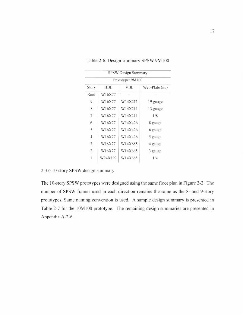
2.3.6 10-story SPSW design summary
The 10-story SPSW prototypes were designed using the same floor plan in Figure 2-2. The
number of SPSW frames used in each direction remains the same as the 8- and 9-story
prototypes. Same naming convention is used. A sample design summary is presented in
Table 2-7 for the 10M100 prototype. The remaining design summaries are presented in
Appendix A-2-6.

18
Table 2-7. Design summary SPSW 10M100
SPSW Design Summary
Prototype: 10M100
Story HBE VBE Web-Plate (in.)
Roof W 16X77 - -
10 W 16X77 W14X257 19 gauge
9 W 14X68 W14X257 13 gauge
8 W 14X68 W14X257 11 gauge
7 W16X77 W 14X257 8 gauge
6 W 14X82 W 14X500 6 gauge
5 W 14X74 W 14X500 5 gauge
4 W 14X74 W 14X500 4 gauge
3 W 18X86 W14X500 3 gauge
2 W14X132 W 14X665 1/4
1 W40X264 W 14X665 1/4

19
Chapter 3. EXISTING METHODS FOR FUNDAMENTAL PERIOD
APPROXIMATION OF SPSW STRUCTURES
The code prescribed methodology for approximating the fundamental period of a structure
is outlined in chapter 12 of ASCE 7-10 [3] as a part of the Equivalent Lateral Force
Procedure (ELFP), the estimated fundamental period is used to calculate the structures
design base-shear. The current code method has been shown to produce overly
conservative estimations of the period for SPSW structures. While AISC 7-10 does allow
the use of a fundamental period obtained through computer analysis this is an impractical
solution. Periods obtained from these types of analysis require the engineer to already have
member sizes selected for the HBE, VBE, and web-plates which are typically unknown in
the preliminary design.
A simplified method to accurately estimate the fundamental period of an SPSW
structure would be a useful tool for a SPSW design. Previous studies have focused on the
development of a simple and accurate method to estimate the fundamental period of SPSW
structures. Two of these methods are considered in this study to serve as a comparison.
This section discusses the current accepted method of approximating a SPSWs
fundamental period. As well the two proposed simplified methods are discussed and
applied to the SPSW prototypes developed for this study.
3.1 Equivalent lateral force procedure
The ELFP, outlined in section 12.8 of ASCE 7-10, is used to calculated the design base-
shear of a structure expressed as
[ASCE 12.8-1] V = CSW (3-1)
where in Eq. (3-1), V is the base shear of the structure; W is the seismic weight of the
structure; and Cs is the seismic response coefficient. The seismic response coefficient is a
parameter which depends on several factors including the location o f the structure,

20
structural system being used, and the fundamental period. The base shear is then
distributed along the height of the structure. Point loading at each level is calculated as
[ASCE 12.8-11] Fx = CvxV (3-2)
In Eq. (3-2), Fx is the point load found at each level, x; CW is the vertical distribution
coefficient. The vertical distribution coefficient determines what percentage of the base
shear will be applied at each level and is calculated for each story as
[ASCE 12.8-12] Cvx = vnW*fe* . fc (3-3)I"= iW iK
In Eq. (3-3), h is the height from the base of the structure to the level of interest; w is the
portion of seismic weight applied to the story of interest; and k is an exponent obtained
from section 12.8.3 of ASCE 7-10. ASCE 7-10 defines k as an exponent related to the
period of the structure [3]. The exponent k is taken as 1 for structures with a period less
than 0.5 seconds and 2 for structures with a period greater than 2.5 seconds. For
intermediate periods between 0.5 and 2.5 seconds the value of k is determined through
linear interpolation. Seismic forces at each level are calculated as
n
[ASCE 12.8-13] Vx = 1 Ft (3-4)i-x
In Eq. (3-4) the seismic force at a particular story is found through the summation of the
story loads found in Equation (3-2) above the level of interest. Applying Eqs. (3-1) through
(3-4) allows the designer to calculate the seismic loads that the structure will need to resist
in order to be code compliant.
3.1.1 Approximation of the fundamental period
The ELFP outlined in Section 12.8 of ASCE 7-10 requires the approximation of the
fundamental period of the structure for the calculation of the base shear described in Eq.
(3-1). It is stated in Section 12.8.2 of ASCE 7-10 that the period of the structure may be
determined from a sufficient analysis using the structural properties and deformation

21
characteristics. This method of analysis requires sizes of the structural elements to be
known, which is generally not the case in the preliminary design stage when the ELFP is
applied. ASCE 7-10 does allow for the use of an approximated formula for the
approximation of a structures fundamental period calculated as
[ASCE 12.8-7] Ta = Cth* (3-5)
In Eq. (3-5), Ta is the approximate fundamental period of the structure; hnis the full height
of the structure; and both G and x are fundamental period coefficients from Table 12.8-2
of ASCE 7-10 [3]. Values for these two coefficients are dependent on the type of LFRS
and are only defined for four LFRSs including steel moment-resisting frames, concrete
moment-resisting frames, steel eccentrically braced frames, and steel buckling-restrained
braced frames. LFRSs not described in Table 12.8-2 are allowed to use the generalized
values for the two coefficients. Values o f G and x are shown below in Table 3-1 for U.S.
customary units. Values of the coefficients are available for the S.I. unit system in ASCE
7-10 Table 12.8-2.
Table 3-1. Values of Period Coefficients Ct and x.
ASCE 7-10 Table 12.8-2 Values of Approximate Period ________________ Parameters Ctand x
Structure Type C, X
Steel moment-resisting frames 0.28 0.8Concrete moment-resisting frames 0.016 0.9Steel eccentrically braced frames 0.03 0.75
Steel buckling-restrained braced frames 0.03 0.75All other structural systems 0.02 0.75
As indicated above, the generalized values of the two coefficients are often used to
approximate the fundamental period of the SPSWs for the use of the ELFP. For the
prototype SPSWs in the previous chapter, Figures 3-1 through 3-3 present the comparison
between the fundamental period using ASCE 7-10 and those from finite element analysis.

22
It can be observed that the use of the generalized values results in overly conservative
estimations.
N100
15r1h
05-
%
15r1to
■aoq3 0 5 “ cl
40
40
40
50
50
50
60
60
60
70 80
M10090 100 110 120 130
70 80
W10090 100
..X.70
Height (ft)
110 120 130
i l . i l 90 100 110 120 130
Finite Element “ — ASCE 7-10
Figure 3-1. Comparison of fundamental period for SPSW prototypes designed with 100
percent base shear.

Perio
d (s
)
23
N85
M85
W85
Finite Element ASCE7-10
Figure 3-2. Comparison of fundamental period for SPSW prototypes designed with 85
percent base shear.

24
N65
96“ 40 50 60 70 80
M6590 100 110 120 130
9 r 40 50 60 70 80
W65
—1_______I_______!_______I_______I90 100 110 120 130
Figure 3-3. Comparison of fundamental period for SPSW prototypes designed with 65
percent base shear.
3.1.2 Seismic response coefficient
The fundamental period of a LFRS is used in the calculation of the seismic response
coefficient, Cs. The coefficient is used to determine what percentage of the seismic weight
will be distributed to the structure as base shear. The seismic response coefficient is
calculated using equation 12.8-2 in section 12.8.1.f of ASCE 7-10. The coefficient is
calculated as
_ Sds[ASCE 12.8-2] ~ ~r ~ (3-6)
VIn Eq. (3-6), G is the seismic response coefficient; S d s is the short period range
design spectral acceleration; Ie is the importance factor; and R is the response modification
factor. Ie is taken from section 11.5 o f ASCE 7-10 and is determined from the inherent risk

25
to human life the structure would have if it were to fail, for this study /<? is taken as equal to
1 for all SPSW prototypes suggesting the structures carry a low risk if it were to fail. R is
a factor which considers the overall ductility of the system; values for R can be found in
Table 12.14-1 in ASCE 7-10, for this study R is taken to equal 7.5 for all SPSW prototypes
suggesting the system will behave in a ductile manner. Sas is a parameter determined from
the geographic location o f the structure; for this study S d s is taken to equal 1.07.
ASCE 7-10 requires checking the seismic response factor calculated in Eq. (3-6)
with a maximum and a minimum value. The minimum value allowed by ASCE 7-10 is
calculated as
[ASCE 12.8-5] Cs = 0.044 S D S I e > 0.01 (3-7)
The maximum allowable value for the seismic response coefficient is calculated as
Sdi[ASCE 12.8-3] Cs ~ ~ R ~ (3-8)
l e
In Eq. (3-8), Sdi is the one second period design spectral response acceleration; and
T is the fundamental period of the structure calculated in Eq. (3-5). As seen in Eq. (3-8) the
maximum value the seismic response coefficient can take is dependent on the period of the
structure calculated using Eq. (3-5). When the overly conservative approximation of the
fundamental period is used the values Cs takes will become larger. A comparison of the
maximum allowed Cs using the fundamental periods from Eq. (3-5) and finite element
analysis are presented in Figures 3-4, 3-5, and 3-6 for the N, M, and W SPSW prototypes
respectfully.

C m
ax
26
Q 4r~
0 2r n*—
0 4j
0
0 4p 0 2b
0*—
3N100
5N100
6N100
10N100
3N85
5N85
6N85
3N65
5N65
6N65
10N85 10N65
lASCE 7-10 ■ F in ite Element
Figure 3-4. Comparison of Cs max values for SPSW N prototypes.
10M100 10M85 10MW65
I ASCE 7-10B|Ftntte Element]
Figure 3-5. Comparison of Cs max values of SPSW M prototypes.

27
OAr0 2 -
oL-0 4r-0 . 2 “
0-0.4«-02-
0-0.2- 0 1 -
0- 0.2- 0 1 -
0-X 0.2rE 0.11-o* 0L
Figure 3-6. Comparison of Cs max values of SPSW W prototypes.
As seen in Figures 3-4, 3-5, and 3-6 the maximum values of Cs calculated using the
fundamental period from finite element analysis are smaller in magnitude when compared
to the values computed using fundamental periods from Eq. (3-5). Using the fundamental
periods from the finite element data would reduce the magnitude of the maximum
allowable Cs potentially reducing the design base-shear of the structure.
3.2 Simplified fundamental period approximation methods
A simple and accurate method for approximating the fundamental period of a SPSW
structure would reduce the iteration during the design process and increase efficiency.
Research has been conducted in the attempt of proposing a simplified method of
approximating SPSW fundamental periods. Two methods are considered in this study,
both of which treat the SPSW as a vertical cantilever and analyze the system as a vibrating
body. These methods are applied to the SPSW and compared with a new method proposed
in this study.
3W100 3W85 3W65
5W100 5W85 5W65
6W100
8W100
6W85
8W85
6W65
8W65
9W100 9W85 9W65
10W1GQ 10W85
|ASCE 7 -1 0 lF in ite Element]
1QW65

28
3.2.1 Approximation method by Liu et al. [11]
A study by Liu et al. [11] proposes a method to estimate the fundamental period of SPSW
structures. In this method, the fundamental period of the structure is approximated by
analyzing both the flexure and shear frequencies using Dunkerley’s equation [17].
Considering the fact that many designers take advantage of the reduction in strength
requirements along the height of the structure and design a SPSW with varying properties
at each story, this method takes into consideration the possibility that the material
properties of the system may not be uniform along the height of the structure.
The shear frequency of the system is calculated from an eigenvalue analysis with
the frame modeled as a lumped mass system [11]. The eigenvalue analysis is calculated
by taking the determinant of the characteristic equation of the system expressed as
[Liu et al. (5)] d e t(K - (OgM) = 0 (3-9)
In Eq. (3-9), M is the mass matrix; K is the stiffness matrix; and tos is the shear frequency.
For a lumped mass system, the mass matrix can be calculated as
M =
m 1000
0m 2
00
00
0 0
... 00 m n
(3-10)
In Eq. (3-10), mn is the story mass at the nth level. The stiffness matrix, K, is similarly
defined as
[Liu et al. (6)] K =
kt + k2 - k 2 k2 k2 + k3
00
0 0 ivn 1V.JJ J
(3-11)
- k n krIn Eq. (3-11) the value kn represents the stiffness of the nth story. It is worth noting that Eq.
(6) in Liu et al. states that a value of -k i should be used for the non-diagonal terms in the

29
first row and first column of the stiffness matrix. It is assumed that this is a simple
typographical error and the correct value of -k2 is therefore used in Eq. (3-11) [18].
The story stiffness used in Eq. (3-11) is a summation of contributions from the
frame and the web-plate. Frame stiffness is determined using the assumption that the
columns are connected to beams with high rigidity as
In Eq. (3-12), kd is the lateral frame stiffness at the ith story; E is the elasticity modulus of
steel; Ic is the moment of inertia of the VBEs; and h is the height of a typical column. The
web-plate stiffness is calculated as
In Eq. (3-13), k pi is the web-plate stiffness at the ith story; L is the bay-width of the SPSW
frame; t is the thickness of the web-plate; and a is the tension field angle. With the stiffness
kci and kpi defined for each story in Eqs. (3-12) and (3-13), the natural frequency of the
SPSW system under shear can be found using Eq. (3-9).
To determine the flexural frequency, the SPSW is modeled as a vertical cantilever
with mass and stiffness uniformly distributed along the height of the structure [11]. The
first mode natural frequency for a cantilever with uniformly distributed mass can be
calculated as [ 19]
In Eq. (3-14), cof is the flexure frequency; H is the full height of the structure; and m is the
distributed mass of the structure taken as the seismic mass divided by the height of the
structure. Using both the natural frequencies of shear and flexure the combined shear-
[Liu et al. (8)] (3-12)
[Liu et al. (9)]E L t
sin2 a cos2 a (3-13)k p i ~ h
[Liu et al. (10 a)] (3-14)

30
flexure frequency can be determined using Dunkerly’s equation [17], which can be
expressed as
0)f[Liu et al. (3)] (i) UUjr UUS
The natural period of the SPSW is then found using the expression
(3-15)
[Liu et al. (4)] T =2nco
(3-16)
3.2.1.1 Application of method by Liu et al.
The method proposed by Liu et al. is applied to the fifty-four SPSW prototypes developed
for this study. The fundamental periods for these SPSW prototypes are shown in Figures
3-4 through 3-6 in comparison with those from ASCE 7-10 and from finite element
analysis. An example o f the method proposed by Lie et a l being used to approximate an
SPSWs fundamental period is presented in Appendix A-3-1.
0L3N100 3N85 3N65
-E Z L T v
%5N100 5N85 5N65
o n_ ; l_[ [_[ l l I
ft
6N100 6N85 6N65
?F8N100 8N85
'zs M l . ' ■■ i
8N65
X ~ 1
o l |0Cl
9N100 9N85 9N65
p - i . ■ •- r - r "
■r / :/ \ ........
; ______________________ P v ^ L 1 ...................
10N100 10N85 10N65F33ASCE 7-10 I [OpenSees Analysis [73 Liu
Figure 3-7. Application of Liu et al. method to 10-foot bay-width SPSW prototypes.

31
?FO'— M -Lfl Z L
?(3M100
l tmm
3M85 3M65
L5M100
E5M85
s a i l ‘ LESS
5M65
6M100
' Li
6M85
* d n s z
6M65
r n P t8M100
f r e t i i ' \ 'EiSi
8M85 8M65
m lyZ 7/
9M100 9M85 9M65
5 i f■c nL_■g °LCLJ 1 l O .
F~/i5, -I u' ;
10M100 10M85 10MW65
Figure 3-8. Application of Liu et al. method to 15-foot bay-width SPSW prototypes.
Pll_______ 1 « i _ J Y lw M 'x.A _______________
3W100 3W85
E X 11
J LI IL3W65
5W100 5W85 5W65
E6W100 6W85
i s i r ± i i 2 a _
6W65
-T ^ n J ' U / I8W100 8W85
E jnijfelJ LEZZI
8W65
j j j ig i] 5 L f ^ v l9W100 9W85 9W65
1 iF r r f t T~ Lf ~ l : i x t . -TSXL10W100 10W85 10W65
Figure 3-9. Application of Liu et al. method to 20-foot bay-width SPSW prototypes.

32
3.2.2 Approximation method by Topkaya and Kurban [13]
A study by Topkaya and Kurban [13] proposed another method for approximating the
natural period of SPSWs. In this method, the fundamental period is determined through
the cyclical natural frequencies of the system under shear and flexure as
[Topkaya (3)] TxW
In Eq. (3-17), Tw is the fundamental period of an SPSW structure; fs is the natural frequency
of the SPSW under shear; and ft is the natural frequency of the SPSW subject to bending.
The natural frequency under bending can be calculated as
r r i rAM r 0.5595[Topkaya (4)] f b = Tf —ElZ^L (3-18)m
In Eq. (3-18), H is the total height of the SPSW structure; E is the elasticity
modulus of steel for the VBE; I is the moment o f inertia of the VBE; m is the distributed
seismic mass of the structure; and rf is a factor proposed by Zalka [14] to take into account
for the lumped mass assumption at each story level. The factor rf is dependent on the total
number of stories of the SPSW structure and is defined for a structure up to 50 stories.
Selected values of rf are shown below in Table 3-2 which encompasses all prototypes of
SPSWs considered in this study.

33
Table 3-2. Values for factor rf
Number of Stories rf1 0.4932 0.6533 0.7704 0.8125 0.8426 0.8637 0.8798 0.8929 0.90210 0.911
The natural frequency of a structure under shear is calculated as
[Topkaya (5)] £ = r / _ L G K A W (3. 19)mN
In Eq. (3-19), G is the shear modulus of steel; and KAW is the effective shear area calculated
as
[Topkaya (6a)] / J (3-20)a A
where the parameter p is calculated as
'Aw Q2[Topkaya (6b)] p = [ j j d A (3-21)
J o b
In Eq. (3-21), Q is the first moment of area of the web-plate; and b is the bay-width of the
SPSW frame. Eq. (3-21) requires integrating polynomials of the fourth degree which is not
practical in a preliminary design stage. An approximation of the value P can be determined
with the assumption that a linear variation exists between Q/b over regions of continuity
[13, 20], where the parameter p is then calculated as

34
[Topkaya (7a)] P = P i + P 2 (3-22)
where Pi is the contribution from the VBE element; P2 is the contribution from the web-
plate. Pi is calculated as
[Topkaya (7b)] A = ~ + ~ d VBE (3-23)
The parameter Qi is calculated as
[Topkaya (7d)] Q i = A f i ( 0 . S p l w + d V B E ) (3-24)
The parameter Q2 is calculated as
[Topkaya (7e)] Q2 = Qi + A w e b 0 . S ( p l w + d V B E ) (3-25)
The contribution from the web-plate is calculated as
[Topkaya (7c)] fe = p l w (3-26)2 p t k
The parameter Q3 is calculated as
[Topkaya (7f)] Q 3 = A V B E 0 . S ( p l w + d V B E ) (3-27)
The parameter Q4 is calculated as
[Topkaya (7g)] Q4 = Q3 + ^ f ^ p t k (3-28)O
3.2.2.1 Application of method by Topkaya and Kurban
The method proposed by Topkaya and Kurban was applied to the SPSW prototypes
developed for this study. It is worth noting that this method was developed for SPSW
frames utilizing the same boundary elements and web-plate along the full height of the
structure. This however is not practical in the design of an optimized SPSW structure as
the strength requirements reduce at each story level allowing reduction in the size of
boundary elements and web-plates [11].

35
To apply this method by Topkaya and Kurban to the SPSW prototypes in this study
a lower bound and upper bound estimation are calculated. The lower bound estimations
are calculated using the VBE and web-plate elements from the bottom level of each
prototype representing the period of the SPSW using the most rigid elements. The upper
bound estimations are calculated using VBE and web-plate elements from the top level of
each prototype representing the period of the SPSW using the least rigid elements. The
results from this method are presented in Figures 3-7 through 3-9 in comparison with those
using ASCE 7-10 and those from finite element method. An example of the method
proposed by Topkaya and Kurban being used to approximate the fundamental period of an
SPSW is presented in Appendix A-3-2.
2r1 -
-iX3N100
ZLl Li
3N85
( J
3N65
5N100
l I L 1..j l
5N85 5N65
6N100
c z l
6N85
JU L
6N65
I rZ L8N100 8N85 8N65
n n:2r
i i£ o
9N100
1ON100
9N85
10N85
9N65
i10N65
2 3 L
| | ASCE 7-10 j | Open Sees Analysis j | Topkaya Upper Bound C M Topkaya Lower Bound
Figure 3-10. 10-foot bay width SPSW results from Topkayas SPSW Fundamental Period
Method.

Perio
d (s
)
36
r m i---- »,— i______ cmU___k ,.K>1 ...........jtttl___li3M100 3M85 3M65
2 r1 -qI----- i—_lJ-----bJ J ® .............. J - l i li , s m ________r— 1..I L M M ......2 -
1 -
5M100 5M85
e h
5M65
6M100 6M85 6M65
8M10G
f ZZL
8M85 8M65
[£E L9M100
EZZL
9M85
fTTl
9M65
10M100 10M85 10MW65
11 [ASCE 7-10 | |openSees Analysis j [Topkaya Upper Bound |' * ] Topkaya Lower Bound
Figure 3-11. 15-foot bay width SPSW results from Topkayas SPSW Fundamental Period
Method.
37
3W100 3W85
1 - ...— ................0 F 'T v l I li m m ............ r ’ - i i — i . ’ E H r ^ r i 1 li BBS
5W12 r
0 I - I f li
00 5W
r— 1 1 1.
85 5W
r ~ i f li
65
m6W1
2r*.......00 6W
j s s i ______i
85
u s r ~ i
6W
i
65
j - ...j___2
10
? 1
lo
8W85
H H i
8W65
9W100 9W85
10W100 10W85 10W85
ASCE 7-10 [ [OpenSees Analysis |Topkaya Upper Bound f v j Topkaya Lower Bound
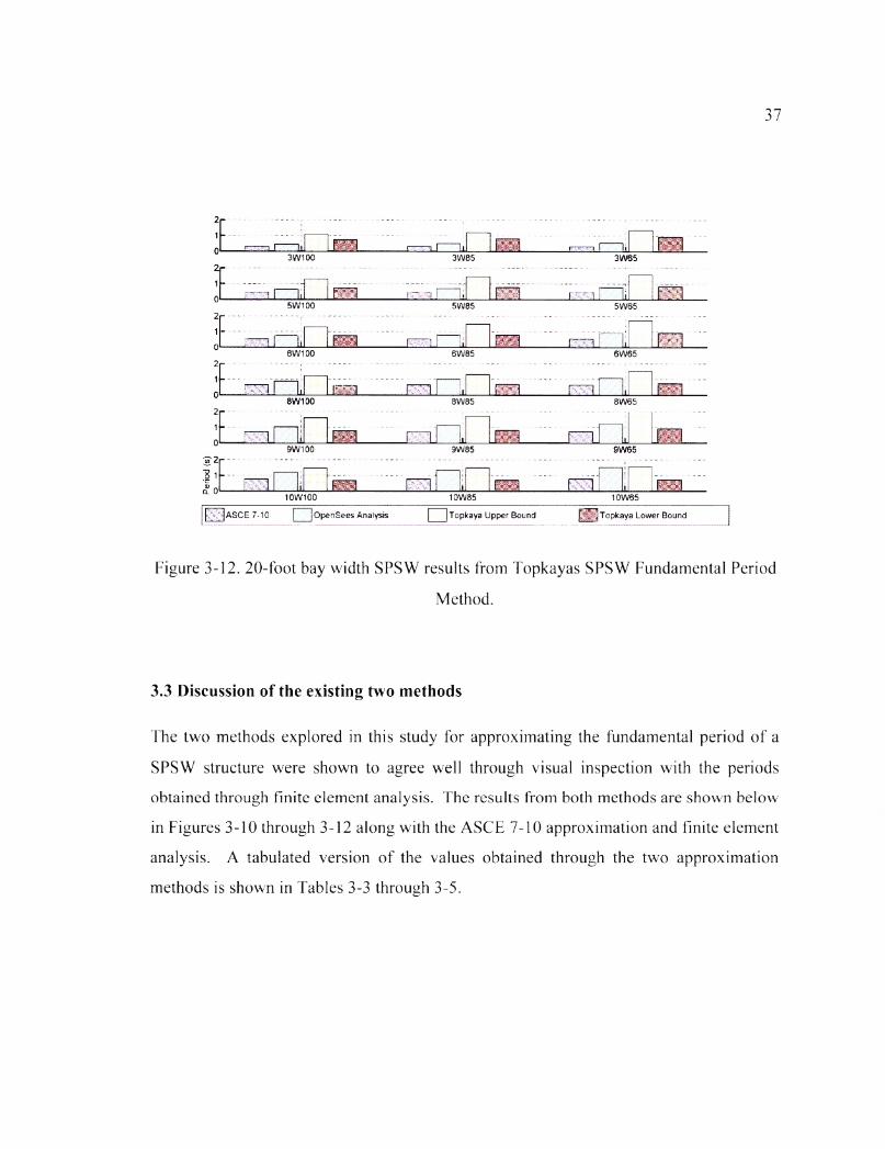
Figure 3-12. 20-foot bay width SPSW results from Topkayas SPSW Fundamental Period
Method.
3.3 Discussion of the existing two methods
The two methods explored in this study for approximating the fundamental period o f a
SPSW structure were shown to agree well through visual inspection with the periods
obtained through finite element analysis. The results from both methods are shown below
in Figures 3-10 through 3-12 along with the ASCE 7-10 approximation and finite element
analysis. A tabulated version of the values obtained through the two approximation
methods is shown in Tables 3-3 through 3-5.

Perio
d (s)
Pe
tiod(
s)
38
2p1 -
3N100lCZL
3N85 3N65
5N100 5N85I I I n n
5N65J__ L
6N100xm J .. ... L
6N85 6N65JZZU
8N100iZILI
8N85i Li
8N65
j | j o9N100 9N85 9N65
A m
10N100jzzu
10N85J— L
10N65f lA S C E 7-10 I ; Open Sees Analysis I iTopkaya Upper Bound HlTopkaya Lower Bound E lL iu
Figure 3-13. 10-foot SPSW period approximations from Liu and Topkaya.
J, Ml ,...L3M100
f ' j...;;,,;,.., ..i3M85
lE h J lE 23M65
2-i ... ........ .0---- t l L l Z I I i lM . .. .... .j— U I n P
I5M100 SM85
J .715M65
J Z l i6M100
-T Li6M85
J L I : : j ~ ~ i □6M65
E U l2f1 -
8M100J---- 18M85
m J8M65
C-...... iVd'tt ' I BO1 “* I
o__ I....L...... j ^ a M l ___ i i n t s i ___ m i i ted9M100 9M85 9M65
X U 10M100 10M85X U
10MW65In A S C E 7-10 ( jQpenSees Analysis I iTopkaya Upper Bound I iTopkaya Lower Bound PSlLiu]
Figure 3-14. 15-foot SPSW period approximations from Liu and Topkaya.

Perio
d (s
)
39
02p1 -0 —
3W100
5W1D0
8W100
9W100
10W100
............ 1
3W85 3W65
[ b £ L.....I I. 1 J— iM L ---------[ m l 1. i_ iJiX l....... ...m l 1,5W85 5W65
I i— i f - ! □n r a r - , r r m m r ~ i c n ® _
2r
1 — r ~ i ____
>W1CX
□0 (5W8e
□awee
r>
8W85 8W65
9W85 9W65
10W85EZL i n i n E - M
10W65[I 1ASCE7-10I OpenSees Analysis I iTopkaya Upper Bound I iTopkava Lower Bound F 'lL iu
Figure 3-15. 20-foot SPSW period approximations from Liu and Topkaya.

40
Table 3-3. 10-foot bay width fundamental period results
Fundamental Period Analysis Method
SPSWPrototype
ASCE 7-10 (s)
Finite Element
Analysis (s)
Upper Bound: Topkaya's Method
(s)
Lower Bound: Topkaya's Method
(s)
Liu'sMethod
(s)3N100 0.499 0.700 0.669 0.512
3N85 0.312 0.566 0.883 0.768 0.571
3N65 0.618 0.953 0.788 0.661
5N100 0.807 0.880 0.495 0.861
5N85 0.458 0.854 0.940 0.532 0.907
5N65 0.952 1.080 0.608 1.017
6N100 0.860 0.870 0.437 0.993
6N85 0.525 0.993 0.884 0.477 1.133
6N65 1.045 0.997 0.533 1.237
8N100 1.245 1.085 0.522 1.358
8N85 0.651 1.303 1.183 0.563 1.420
8N65 1.491 1.293 0.673 1.657
9N100 1.334 1.192 0.510 1.515
9N85 0.711 1.521 1.269 0.580 1.734
9N65 1.543 1.269 0.580 1.745
10N100 1.583 1.203 0.555 1.799
10N85 0.770 1.722 1.405 0.563 1.972
10N65 1.940 1.475 0.686 2.176

41
Table 3-4. 15-foot bay width fundamental period results
Fundamental Period Analysis Method
SPSWPrototype
ASCE 7- 10 (s)
Finite Element
Analysis (s)Upper Bound:
Topkaya's Method (s)Lower Bound:
Topkaya's Method (s)Liu's
Method (s)
3M100 0.469 0.953 0.944 0.518
3M85 0.312 0.512 1.018 0.782 0.573
3M65 0.564 1.100 0.806 0.667
5M100 0.710 1.053 0.611 0.832
5M85 0.458 0.753 1.200 0.685 0.887
5M65 0.872 1.391 0.744 1.023
6M100 0.812 1.141 0.644 0.960
6M85 0.525 0.895 1.281 0.704 1.065
6M65 0.957 1.408 0.763 1.1398M100 1.124 1.366 0.664 1.278
8M85 0.651 1.171 1.440 0.701 1.332
8M65 1.332 1.647 0.808 1.530
9M100 1.146 1.423 0.643 1.296
9M85 0.711 1.200 1.514 0.712 1.331
9M65 1.429 1.772 0.816 1.641
10M100 1.378 1.295 0.604 1.555
10M85 0.770 1.473 1.645 0.715 1.664
10M65 1.675 1.597 0.734 1.904
42
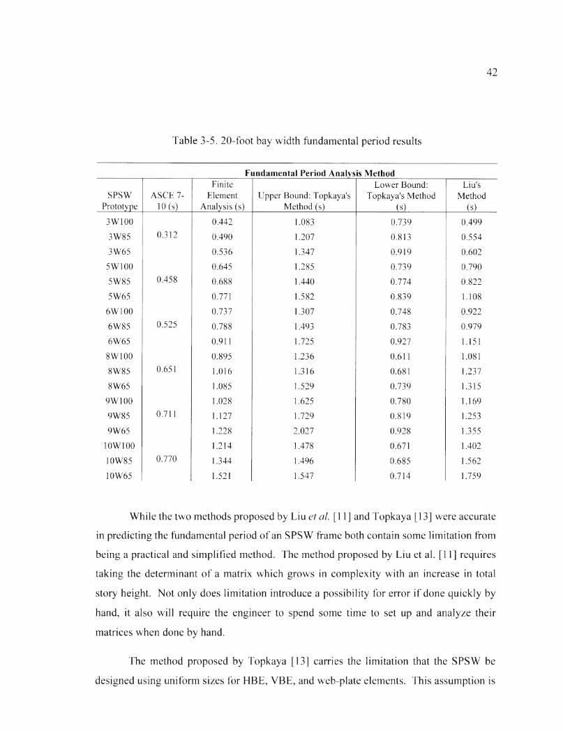
Table 3-5. 20-foot bay width fundamental period results
Fundamental Period Analysis Method
SPSWPrototype
ASCE 7- I 0 ( s )
Finite Element
Analysis (s)Upper Bound: Topkaya's
Method (s)
Lower Bound: Topkaya's Method
(s)
Liu'sMethod
(s)3W100 0.442 1.083 0.739 0.4993W85 0.312 0.490 1.207 0.813 0.5543W65 0.536 1.347 0.919 0.602
5W100 0.645 1.285 0.739 0.7905W85 0.458 0.688 1.440 0.774 0.822
5W65 0.771 1.582 0.839 1.108
6W100 0.737 1.307 0.748 0.922
6W85 0.525 0.788 1.493 0.783 0.979
6W65 0.911 1.725 0.927 1.151
8W100 0.895 1.236 0.611 1.081
8W85 0.651 1.016 1.316 0.681 1.237
8W65 1.085 1.529 0.739 1.315
9W100 1.028 1.625 0.780 1.169
9W85 0.711 1.127 1.729 0.819 1.253
9W65 1.228 2.027 0.928 1.355
10W100 1.214 1.478 0.671 1.402
10W85 0.770 1.344 1.496 0.685 1.562
10W65 1.521 1.547 0.714 1.759
While the two methods proposed by Liu et al. [11] and Topkaya [13] were accurate
in predicting the fundamental period of an SPSW frame both contain some limitation from
being a practical and simplified method. The method proposed by Liu et al. [11] requires
taking the determinant o f a matrix which grows in complexity with an increase in total
story height. Not only does limitation introduce a possibility for error if done quickly by
hand, it also will require the engineer to spend some time to set up and analyze their
matrices when done by hand.
The method proposed by Topkaya [13] carries the limitation that the SPSW be
designed using uniform sizes for HBE, VBE, and web-plate elements. This assumption is

43
not practical especially when designing an SPSW greater than 3 stories. While the upper
and lower bound estimations provide a range where the engineer can approximate the
period it does not give a definite value to use in the design.

44
CHAPTER 4. FINITE ELEMENT MODELING OF SPSW
PROTOTYPES
This chapter discusses the finite element modeling and analysis for the fundamental period
o f the SPSW prototypes.
4.1 Open System for Earthquake Engineering Simulation (OpenSees)
For this study SPSW prototypes were modeled and analyzed using the software platform
Open System for Earthquake Engineering Simulation (OpenSees). OpenSees is open
source software produced by the Pacific Earthquake Engineering Research (PEER) Center
for modeling and analyzing the nonlinear response of structural systems. For this study
OpenSees version 2.4.6 was used for all modeling and analysis of the SPSW prototypes
[21]. OpenSees analysis was performed to obtain the fundamental period for each SPSW
prototype using the Eigen algorithm [22].
4.2 Modeling of SPSW Prototypes
The finite element models used in this study were based on models previously used in
studies at San Francisco State University performed by Enright [8] and Barghi [9]. For
specific modeling questions the OpenSees Wiki [23] was utilized.
Web-plate modeling was achieved using the strip method outlined in AISC Design
Guide 20 [1]. The strip method models the web-plate as a series of pined tension only truss
members which are placed diagonally along the HBE. The truss members are modeled to
have a significant tension capacity and negligible compression strength. To achieve the
effects o f the distributed loading that the web-plate acts onto the HBE member AISC
recommends at least ten strips be used in each direction when modeling the web-plate. A
visualization of the strip method is provided below in Figure 4-1.

45
Th1
y y y y / ^
:Y / .Y vf> ...................... A i
■------------L-------------
Figure 4-1. Visualization of the strip method [1].
The web-plate tension strips are modeled so their angle matches closely to the
tension-field angle, a, shown in Figure 4-1. Tension strips are assumed to be distributed
along the HBE using similar node locations for each story level. This is a simplifying
assumption as the tension-field angle will slightly vary at each story level. An average of
the tension field angles at each level are taken when determining how many tension strips
to use for web-plate modeling. This technique is allowed by AISC Design Guide 20 but is
only recommended when bay-width and story heights are similar, which is the case for the
prototypes used in this study [1].
Determining the number of tension strips to use for the web-plate modeling was
done based on work by Barghi [8]. Tension strips were selected so that diagonal of each
strip would lie within a 5% tolerance o f the average tension field angle used for each SPSW
prototype. Using this requirement, the number of strips in each direction fell between 15

46
and 16 for each prototype. Figure 4-2 shows a 6-story OpenSees model whose setup is
typical for all prototypes.
VBE and HBE elements were modeled so that plasticity was distributed along the
length of the member. This was done so that the tension effects o f the truss pulling at
different locations on the members would be accurately modeled.
4.3 Panel zone modeling
Panel zones at beam-to-column connections were modeled using an algorithm provided by
Lingos [24] which is based on definitions provided by Gupta et al. Modification of Lingos
algorithm was required for the 10-story SPSW prototypes due to node conventions used by
OpenSees. A visualization of a typical OpenSees Panel Zone configuration is shown in
Figure 4-3.

47
Rotational Spring (element 4xy00)500xyl x
[xy02] _ A |xy03][xy04]- 500xy3
[xyOl]500xy8 — - - — 500xy3
« [Xy'° \x y05] -500xy7 - — 500xy4
[xy091 I[xy08] |
500xy6 —
Figure 4-3. Visualization of a typical panel zone configuration at beam-to-column
connection.
The panel zones at beam-to-column connections are modeled similarly to the
configuration shown in Figure 4-3. Coordinates xyOl through xylO represent the node
locations defined by the user to create the location for each panel zone. The variable x
represents the pier each panel zone is being defined on. The variable y represents the story
level where each panel zone is being defined. Panel zone elements are modeled using eight
beam-column elements which carry a very high stiffness represented by elements 500xyl
through 500xy8 in Figure 4-3 [25].
The configuration shown in Figure 4-3 was used for all SPSW models excluding
the 10 story SPSW prototypes. An error in modeling the 10 story SPSW prototypes
presented itself when the panel zones and tension strips were defined at the roof level. The
source of error was found to be from the node conventions used by OpenSees to define the
locations of both the tension strips and panel zones. To remove this error, the node
conventions used for defining the panel zone locations were modified.

48
To visualize the source of this error, Figure 4-4 shows the typical convention for
defining nodes on the SPSW HBE elements. The variable n represents the story being
modeled. When the top level o f the 10 story SPSW prototypes were being modeled in
OpenSees the node coordinates of nOOl with n equal to 10 was required resulting in a node
coordinate of 10001. Based on the panel zone node definitions shown if Figure 4-3 and
the beam node definitions shown in Figure 4-4 an identical node of 11005 is generated
when modeling the first pier, tenth story panel zone and the roof HBE. OpenSees is not
capable to distinguish the difference between the two different nodes and was unable to
run any analysis using the algorithms for the previous models.
To account for this error, the panel zone source code was modified at the top two
HBE elements. Modifying the code was accomplished by inserting an additional zero at
the node coordinate to distinguish it from the node defined on the HBE. This required
modifying the OpenSees source code [24] to account for the additional zero. The modified
code used for the 10 story SPSW models is provided in Appendix A-4-1. A visualization
of the modified panel zone configuration is shown below in Figure 4-5.

49
Figure 4-5. Configuration of the modified panel zones.
The configuration presented in Figure 4-5 was adopted into the 10-story SPSW
finite element models. Once adopted the Eigen analysis was able to converge and the
fundamental period was computed.

50
Chapter 5. STATISTICAL ANALYSIS
To develop a more efficient method for approximating the fundamental period of SPSWs,
a statistical analysis is performed with MATLAB [25] using fundamental period data
obtained from the SPSW prototypes presented in Chapter 2. The objective of this analysis
is to develop adjustment expressions to better approximate the fundamental period
coefficients, Ct and x, used in Eq. (3-5). This method is developed so that the bay-width
and the base-shear participation level of the structure are the only parameters required.
These parameters are typically known to the designer when calculating seismic loads
making it ideal for application in the initial design stage of SPSWs. In this section, a method
for approximating the fundamental period coefficients of SPSWs is developed and
proposed. Adjustment expressions are first developed considering only the bay-width of
the prototypes; expressions are then developed to adjust the bay-width expressions
according to the structures base-shear participation levels.
5.1 Statistical analysis of the SPSW prototypes
ASCE 7-10 Eq. (12.8-7) approximates the fundamental period as a power function of the
structure height as shown in Eq. (3-5). It was assumed for the development o f the proposed
method that the periods obtained from the finite element analysis would follow a similar
trend to be behavior of Eq. (3-5). Using MATLAB [27] a first-degree power regression
was performed assuming the data to follow the following form:
y = a x b (5-1)
where in Eq. (5-1) the coefficients a and b represent the fundamental period coefficients Ct
and x, respectfully; the variable y represents the fundamental period of the system in
seconds; and x represents the height of the structure in feet. Shown in Figure 5-1 is a
comparison of the regression analysis and the finite element analysis. Table 5-1 gives
tabulated values of the coefficients a and b obtained from the regression analysis.

51
N100 N85 N652 2
1.5 . / . 1 5
1 1
0 5 _______ 0.5150 150M100 M85
50 100M65
150
151
05
Q 50 100W100
150
151
05
0,50 100
W85150
2
151
0 5,50 100
W65150
1.5
' 1a> 0 5 a.
15 2
£ 1 3q> 0 5Q-
n
Perio
d (s
.........
Height (ft)150
Height (ft)150
Height (ft)150
| — Power Regression Finite Element
Figure 5-1. Comparison between periods from regression and finite element analysis.
Table 5-1. Fundamental period coefficients from regression analysis.
SPSW Prototype C, X
N100 0.0125 0.9877
N85 0.0144 0.9774
N65 0.0153 0.9839
M100 0.0159 0.9097
M85 0.0192 0.8828
M65 0.0175 0.9312
W100 0.0181 0.8534
W85 0.0174 0.8833
W65 0.0197 0.8786
As seen in Figure 5-1 the power regression models the behavior of the finite
element analysis closely. This suggests that the assumed behavior described in Eq. (5-1)
appropriately models the behavior of the fundamental period of a SPSW. The G and x
coefficient values presented in Table 5-1 are derived using only the height of the structure

52
as a parameter. To adjust the fundamental period coefficients to their assumed correct
value, adjustment functions for Ct and jc are derived first only considering the bay-width of
the structure as a parameter. For this only SPSW prototypes designed for 100 percent base-
shear participation were considered. An additional expression adjusting the coefficients
considering the base-shear participation of the structure using the remaining SPSW
prototypes is then presented.
5.2 Bay-width adjustment function
5.2.1 Ct bay-width adjustment function
The Ct adjustment function for bay-width is assumed to take the form
where, Ct' is the adjusted fundamental period coefficient; G is the code prescribed value
taken from ASCE 7-10t; and f c {L) is the bay-width adjustment function.
To determine the form of the Ct adjustment function Eq. (5-2) can be modified as
Using Eq. (5-3), values for f c (L) can be calculated for the bay widths considered in this
study using SPSWs designed for 100 percent base-shear participation. Table 5-2 gives
values o f / c (L)at the considered bay-widths.
c l = Ctfc(U) (5-2)
(5-3)l a s c e
Table 5-2. /(L ) values for fundamental period coefficient fc(L).
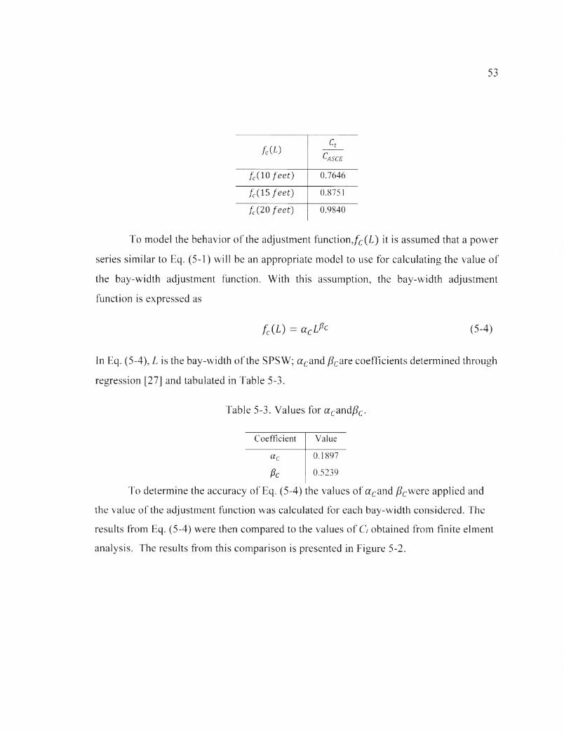
53
Ctfo il)
l a s c e
/c(10 fe e t ) 0.7646
fc( 15 f e e t ) 0.8751
A (20 f e e t ) 0.9840
To model the behavior of the adjustment function,/C(L) it is assumed that a power
series similar to Eq. (5-1) will be an appropriate model to use for calculating the value of
the bay-width adjustment function. With this assumption, the bay-width adjustment
function is expressed as
U L ) = cccLPc (5-4)
In Eq. (5-4), L is the bay-width of the SPSW; a cand /?care coefficients determined through
regression [27] and tabulated in Table 5-3.
Table 5-3. Values for a cand/?c .
Coefficient Value
«c 0.1897
Pc 0.5239
To determine the accuracy of Eq. (5-4) the values of a cand /?cwere applied and
the value of the adjustment function was calculated for each bay-width considered. The
results from Eq. (5-4) were then compared to the values of G obtained from finite elment
analysis. The results from this comparison is presented in Figure 5-2.

54
0,054
0 052
0 05
0 048
O0 046
0.044
0 042
0 04 35j ’ —Finite Element Coefficient Adjustment Function Coefficient t
45 5Bay Width (ft)
55 65
Figure 5-2. Comparison of adjusted G values and finite element values.
As seen in Figure 5-2 the Ct values using Eq. (5-4) can acceptably model the
behavior of Ct values taken from the finite element analysis. From a visual inspection, it
can be assumed that behavior o f the adjustment function described in Eq. (5-4) is an
accurate model to use.
5.2.2 x bay-width adjustment function
The derivation of the adjustment function for the coefficient x used in Eq. (3-5) is
performed in a similar fashion to the Ct adjustment function derived in the previous section.
The adjustment of x to the regression values presented in Table 5-1 was performed
assuming the following expression
x' = xfx(L) (5-5)
where in Eq. (5-5), x' is the adjusted value of the fundamental period coefficient; x is the
code prescribed value obtained from ASCE 7-10; and fx(L) is the bay-width adjustment
function. To determine the appropriate model to use for describing the behavior o ffx(L),

55
values were computed at the SPSW bay-widths similar to the procedure presented in Eq.
(5-3) and are presented in Table 5-4.
Table 5-4. Values of fx{L) at considered SPSW bay-widths.
/*(£) X
XASCE
fx( 10 fe e t) 1.3118
fx{ 15 fe e t) 1.2416
A (20 fe e t ) 1.1714
The behavior of fx(L) is assumed to behave similar to f c {L) in Eq. (5-4) and can
be expressed as
/ , ( i ) = axLV* (5-6)
where in Eq. (5-6), L is the bay-width of the SPSW in feet; a* and /?xare coefficients found
through a power regression analysis in MATLAB [27] and are presented in Table 5-5.
Table 5-5. Coefficient values for the adjustment functionfx(L).
Coefficient Value
2.1368
Px -0.2099
To determine if Eq. (5-6) is an appropriate model to use adjusted values o f x using
Eq. (5-6) were computed and compared with the x values obtained from the finite element
analysis. This comparison is presented in Figure 5-3.

1 — Finite Element CoefHcient — Adjustment Function Coefficient ! . , . .Q = ^ ; v : .= == = = === i-------- 1-------------------------------- 1-------------------------------- 1--------------------------------- 1
3 3 5 4 4 5 5 5 5 6 6 5Bay Width (ft)
Figure 5-3. Validation of power series assumption for jc coefficient adjustment function.
As seen in Figure 5-3, the model presented in Eq. (5-6) is able to closely
approximate the adjusted values of x to those computed from the finite element analysis.
Therefore, Eq. (5-6) is used for adjusting the coefficient x according to the bay-width of
the structure.
5.3 Derivation of base-shear participation adjustment function
Current code provisions require the web-plate of the SPSW to be designed to resist 100
percent of the design-base shear [1], Previous studies conducted by Berman, Enright, and
Bhargi [9,5,6] suggest that the boundary elements in the SPSW can add substantial strength
to the system which is currently ignored. If this additional strength is considered in the
design a reduction in base-shear resisted in the web-plate will be conducted to optimize the
system. The reduction in base-shear resisted in the web-plate due to the plate-frame
interactions were considered in the study with SPSW prototypes being designed for 85 and

57
65 percent of the design base shear in addition to the code prescribed 100 percent
prototypes.
The adjustment functions derived in the previous sections adjust the fundamental
period coefficients, G and x, used in Eq. (3-5) with the bay-width of the SPSW as the only
parameter. To continue exploring the effects of reducing the design base-shear in the web-
plate additional adjustment functions are developed considering a possible variation in the
base-shear participation ratio. These expressions are developed adjusting the a and P
coefficients derived in Eqs. (5-4) and (5-6) based on the design base-shear resisted in the
web-plate.
5.3.1 G base-shear adjustment function.
The adjusted fundamental period coefficient Ct' is expressed as:
where in Eq. (5-7), a cand /?care the bay-width adjustment coefficients whose values are
taken from Table 5-3. To account for a variation in the design base-shear resisted in the
web-plate, adjustment functions for both a cand /?c are derived and presented in this
section.
The behavior of the adjustment functions for a cand /?c are assumed to be modeled
similar to Eq. (5-2) and are expressed as:
C' = Cta cLPc (5-7)
a'c = a cfac ( y ) (5-8)
Pc = PcfficQO (5-9)
The expressions fa (V) and fpc (V) in Eqs. (5-8) and (5-9) are found in a similar
way to / c ( i ) in Eq. (5-3). Values o f fac(V) and fpc (V) at each base-shear participation
ratio considered in this study are presented in Tables 5-6 and 5-7, respectively.

58
Table 5-6. fac(Y) at base-shear participation ratios.
/«c0 0Cioo
/«c(ioo% ) 1
fac (85%) 2.2146
foci 65%) 1.7313
Table 5-7. fpc(V) at base-shear participation ratios.
fficOO «c
ac100
fpc( 100%) 1
fpci 85%) 0.5019
fpci 65%) 0.6967
To determine the appropriate model to use for describing the behavior o f the
adjustment functions over the considered base-shear participation ratios a visual inspection
was performed for both fac(V) and fpc(V). For this inspection values of a cand /?c were
computed for each considered base-shear participation level and plotted over the base-shear
participation ratios. The results from this inspection are presented in Figures 5-4 and
Figures 5-5, respectively.

alph
^.
59
Base-Shear Participation
Figure 5-4. ac over base-shear participation levels.
Figure 5-5. Pc over base-shear participation levels

60
As seen in Figures 5-4 and 5-5 a visual inspection of the adjusted coefficients over
the base-shear participation levels gives no explicit model to accurately describe the
behavior of the data. Therefore, two models are presented and explored to determine the
appropriate form of the base-shear adjustment function. Both models are presented in this
section and later analyzed to determine the appropriate model to use for describing the
behavior of the adjustment functions. The first model assumes the adjustment functions
fac (V) and fp (V) to be modeled as a power series similar to Eqs. (5-6) and (5-7),
expressed as:
fa cOO = (5-1°)ftcQO = e/cv ri,c (5-ii)
In Eqs. (5-10) and (5-11), V is the base shear participation ratio;0ac, yac, 6pc, and
Ypc are coefficients whose values are determined through power series regression in
MATLAB [27]. Values for 6ac, yac, 0pc, and ypc assuming the form presented in Eqs. (5-
10) and (5-11) are provided in Tables 5-8 and 5-9 for fac(V) and fpc(V), respectively.
Table 5-8. Values for 6ac and yac assuming a power series model.
fa c (Y y coefficient value Value
1.493
Vac -0.691
Table 5-9. Values for °Pc and Ypc assuming a power series model.
fpc (K ) coefficient value Value
dPc 0.870
YPc 0.948

61
The second model considered assumes the adjustment functions fac(V) and
fpc(V) to vary linearly over the base-shear participation ratios. With this assumption fa (V)
and fpc (K) are expressed as
fac(V) = eacV + Yac (5- 12)
fpc (v ) = dPcV + Ypc (5_13)
In Eqs. (5-12) and (5-13), V is the base-shear participation ratio; 9ac, yac, 9pc, and
Ypc are coefficients whose values are determined through a linear regression in MATLAB
[28]. Values for 6ac, yac, 6pc, and ypc assuming the form presented in Eqs. (5-12) and (5-
13) are provided in Tables 5-10 and 5-11 for fac(V) and fpc(V), respectively.
Table 5-10. Values for Gac and yac assuming a linear variation.
fa (V) coefficient value Value
0 «c -1.846
Yac 3.187
Table 5-11. Values for 6pc and ypc assuming a linear variation.
fpc ( I /) coefficient value Value
0.7671
YPc 0.0937
5.3.2 x base-shear adjustment function.
A similar procedure is used for the derivation of a base-shear participation adjustment
function for x to that of Ct. The adjusted fundamental period coefficient x' is expressed as:
x' = xaxL^x (5-14)

62
where in Eq. (5-14), a xand /?x are coefficients whose values are obtained through
regression analysis and are presented in Table 5-5. To account for a possible variation in
base-shear resisted in the web-plate, additional adjustment functions are derived for a xand
(3X considering the variation of base-shear participation ratios considered in this study. The
adjusted values of the coefficients a^and j3x are assumed to take the form:
a'x = ocxfax(V) (5-15)
P x = P x f p x GO (5-16)
To determine the behavior o f fUx(V) and fpx(V), values of a xand /3X are calculated
at each base-shear participation level considered in this study, tabulated values are
presented in Tables 5-12 and 5-13, respectively.
Table 5-12. Values of fa (V) at varying base-shear participation levels.
fax 0 0 ax
aXioo
/ax(100%) 1
fax (85%) 0.8663
faxi 65%) 0.8905
Table 5-13. Values of fpx(V) values at each base-shear participation value.
/fe(v0“ *100
/ fe (100%) 1
/& ( 85%) 0.7471
/fc ( 65%) 0.7641

alph
^
63
To determine the appropriate model to use for describing the behavior of a x and
(3X ,the values of ax and (3X at each base-shear participation level are computed and plotted
over the varying base-shear participation levels and presented in Figures 5-6 and 6-7.
Figure 5-6. Variation of axover base-shear participation levels.

64
Figure 5-7. Variation of |3x over base-shear participation levels.
As seen in Figures 5-6 and 5-7, the appropriate model to use for describing the
behavior of axand (3X is not explicitly given. Similar to a c and /3C, two models are
presented and later analyzed to determine the appropriate to use.
The first model assumes the adjustment function to behave as a power series. Using
this assumption, the adjustment functions fa (V) and fpx(V) are expressed as
fax0 0 = 0 « V Ya* (5-17)
fpx(V ) = dpVVPx (5-18)
In Eqs. (5-17) and (5-18), Vis the base-shear participation level; and 0Ux, yUx, Qpx,
and y ^are coefficients obtained through a power regression analysis in MATLAB [27].
Tabulated values of 6Ux, yUx, 0px, and y ^are provided in Tables 5-14 and 5-15 for fUx(V)
and fp QT), respectively.

65
Table 5-14. Values for 9Uxand /^assum ing a power series variation.
fax (V) coefficient value Value
0.9642
Yax 0.2484
Table 5-15. Values for 9px and yp assuming a power series variation.
fpx ( 7 ) coefficient value Value
dPx 0.9420
Ypx 0.6304
The second model assumes a linear variation over base-shear participation ratios.
Under this assumption f a (V) and fp (V) are expressed as
/ o ,0 0 = K V + fax (5-20)
f e W = ek v + Yh (5-2i)
where in Eqs. (5-20) and (5-21), V is the base-shear participation ratio; and the
coefficients 9Ux, yUx, 9px, and yp are obtained through a linear regression analysis in
MATLAB [28]. The values of 9Ux, yUx, 9px, and y^are shown in Tables 5-16 and 5-17 for
fax(V) and fpx(V), respectively.
Table 5-16. Values for 9Ux and ya% assuming a linear variation.
/^^(F)coefficient value Value
0.2894
Yax 0.6777

66
Table 5-17. Values for 0px and Ypx assuming a linear variation.
fp ( V ) coefficient value Value
0.6331
ypx 0.3095
5.3.3 Error analysis of base-shear adjustment function models
The model to describe the base-shear adjustment function was not explicitly given from
the visual inspections performed in Figures 5-4 through 5-7. Both a power series model
and a linear series modeled were considered. To determine which of these two models are
more appropriate to use an error analysis in the form of the root mean squared method was
performed using MATLAB [29]. Results from the error analysis are tabulated in Table 5-
18.
Table 5-18. Root Mean Squared Analysis results for the power series and linear model.
Root Mean Squared Error Analysis
Structure
Class
Power Series
model
Linear
Model
N100 0.2191 0.1414
N85 0.0864 0.0939
N65 0.1007 0.0751
Ml 00 0.1448 0.0783
M85 0.0775 0.0844
M65 0.1113 0.069
W100 0.1605 0.0971
W85 0.0676 0.0746
W65 0.0868 0.0642
As seen in Table 5-18, the linear model for the base shear adjustment function is
more appropriate for modeling the behavior of the SPSWs fundamental period

67
coefficient. From this observation the linear models presented in Eqs. (5-12), (5-13), (5-
20), and (5-21) will be adopted for the proposed method.
5.4 Proposed method for approximating the fundamental period
Based on the derivations outlined in this chapter the proposed method of approximating
the fundamental period of an SPSW prototype can be summarized as
T = Ctf c (L)Hxf* V (5-22)
fc(L) = a cfacm L M >cm (5-23)
fx(L) = axfXc(V )L^I>,m (5-24)
fac(.V) = e„cV + Yac (5-12)
ff,c{V) = V + Yt>c (5-13)
faxm = eaxv + (5-20)
+OSII (5-21)
Tabulated values for all variables used in the method are presented in Table 5-19.
The method proposed in this section was applied to the SPSWs developed for this study.
The fundamental period of the SPSWs using the proposed method are compared with the
fundamental periods obtained from the finite element analysis. This comparison is
presented in Figure 5-8.

68
Table 5-19. Parameter values for proposed methods.
Parameter Value1
Q 0.02(0.0488)
X 0.75(0.75)
«c 0.1897(0.6016)
Pc 0.5239(0.2979)
2.1368(1.6652)
Px -0.2099(-0.2099)
-1.8S6<-0.9681>
Vac 3.187(2.0747)
0.7671(0.9767)
ypc 0.0937(-0.1457)
6 a ax 0.2894(0.1442)
Yax 0.6777(0.8355)
0.6331(0.6331)
y p x 0.3095(0.3095)
'S.I. equivalents are given in parenthesis

69
N100
0
1 5f
1
05
0
1 5f
3 1ES 0.5Q,
qo
50 100M100
150
50 100W100
150
1 5-
1 ■
1 5
1
05
q
1 5
H 1 E§ 0.5
50 100Height (ft)
150
N85
50 100M85
N65
50 100W85
50 100Height (ft)
150
150
2'15
1
2
1 5
10 5,
150
E 1 S
CL.
0,
50 100M65
50 100W65
150
150
50 100 150 ________ Height (ft) .........- —Proposed Function Finite Element Period;
Figure 5-8. Results from application of proposed method on SPSW prototypes.
As seen in Figure 5-8, the proposed method can closely approximate the
fundamental period of the SPSWs designed for this study when compared to the finite
element analysis. From this comparison, it can be concluded that the proposed method
can be used to approximate the fundamental period of an SPSW if designed similar to the
prototypes developed for this study.

70
CHAPTER 6. VALIDATION OF PROPOSED METHOD
To determine the validity of the proposed method, SPSWs with story heights, bay-widths,
and base-shear participation ratios not considered in the initial population. The SPSW
validation prototypes were designed using the specification from AISC Design Guide 20
[1]. Finite element modeling and analysis of the fundamental period was performed using
OpenSees [23]. The fundamental period of the prototypes were then obtained using the
proposed method and compared with the finite element analysis.
6.1 SPSW validation prototypes
Three SPSW prototypes were designed for the validation of the method proposed in this
study. The validation prototypes include a three story, twelve-foot bay-width SPSW with
a 100 percent base-shear participation ratio denoted 3K100; a four story, ten-foot bay width
SPSW with an 80 percent base-shear participation ratio denoted 4N80; and a seven story,
twenty-foot bay width SPSW with a 60 percent base-shear participation ratio denoted
7W60. Design summaries for each validation prototype are presented below in Tables 6-1
through 6-3.
Table 6-1. 3K 100 SPSW design summary
Design Summary: 3K100
Story HBE VBE Web-Plate
Roof W 18X65 - -
3 W 18X65 W 14X233 15 gauge
2 W16X57 W 14X233 11 gauge
1 W24X250 W 14X233 9 gauge

71
Table 6-2. 4N80 SPSW design summary
Design Summary: 4N80
Story HBE VBE Web-Plate
Roof W 14X68 - -
4 W 14X68 W14X145 18 gauge
3 W 14X68 W14X145 13 gauge
2 W14X68 W14X233 11 gauge
1 W 18X65 W 14X233 10 gauge
Table 6-3. 7W60 SPSW Design Summary
Design Summary: 7W60
Story HBE VBE Web-plate
Roof W18X119 - -
7 W18X119 W14X132 23 gauge
6 W18X119 W 14X233 17 gauge
5 W18X119 W 14X23 3 14 gauge
4 W 18X65 W 14X233 12 gauge
3 W 18X65 W 14X45 5 12 gauge
2 W 14X53 W 14X45 5 11 gauge
1 W24X306 W 14X45 5 11 gauge
6.2 Results from approximation method.
The method proposed in this study was applied to the three validation prototypes and then
compared with the results from a finite element analysis results. Tabulated values from the
proposed method and finite element analysis comparison are given in Table 6-5. The
comparison is presented in Figures 6-1 through 6-3.
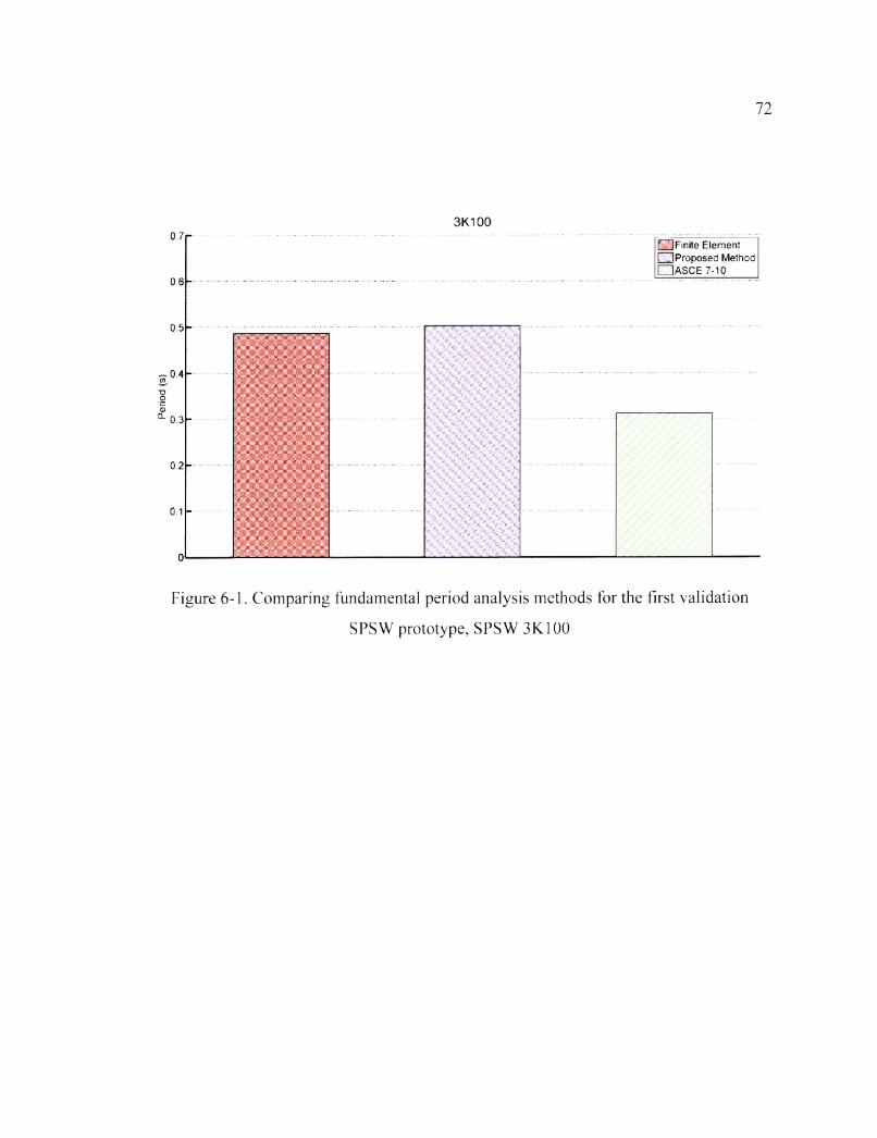
Perio
d (s
)
72
3K1000.7
0.6
0.5
0.4
0.3
0.2
0 1
p.A. * ■
- .
H i Finite Element mProposed Method □ A S C E 7-10
Figure 6-1. Comparing fundamental period analysis methods for the first validation
SPSW prototype, SPSW 3K100

Perio
d (s
)
73
4N800.8r
0,7-
0 6 -
0.5-
0 4 -
0.3-
02-
0.1
' " "* “ . M*' *" S''1*'*VVvvVV/y-v
' V V X % <V\ *V*/,v%'VvS.\
> x x v
XV«LiV %%:*
F I Finite Element ( I Proposed Method □ A S C E 7-10
Figure 6-2. Comparing fundamental period analysis methods for the second validation
SPSW prototype, SPSW 4N80

74
7W60
i fkmW
■ ■ /■/-> .. '
.■ ■ . ■ ■ ■ ,
* A \■ >
□ Finite Element □Proposed Method □ A S C E 7-10
Figure 6-3. Comparing fundamental period analysis methods for the third validation
SPSW prototype, SPSW 7W60.
Table 6-4. Comparison of fundamental periods from finite element analysis and the
proposed method for the three validation prototypes.
Comparison of Fundamental Period Analysis for Validation SPSW PrototypesSPSW
Prototype Finite Element Period (s) Proposed Method Period (s) Error3K100 0.486 0.503 3.50%4N80 0.738 0.731 0.95%7W60 1.003 1.017 1.40%
As seen in Figures 6-1 through 6-3 the proposed method is able to closely
approximate the fundamental period of an SPSW when compared to a finite element
analysis.

75
6.3 Summary
In this study the fundamental period of fifty-four SPSW structures was used to develop a
simplified method for approximating the fundamental period. The proposed method
approximates by adjusting the fundamental period coefficients to use in ASCE 7-10
equation 12.8-7 for a SPSW structure based on the bay-width and base-shear participation
level. The method proposed in this study is summarized as follows in Eqs (6-1) through
(6-7).
T = Ctf c (L)Hxf*M (6-1)
fc ( 0 = a cfac(V)LPcfec(v) (6-2)
fx ( 0 = axfXc( V ) L ^ f ^ (6-3)
fac (V) = dacV + yac (6-4)
fpcW = ePcV + Ypc (6-5)
fax(V) = da V + Yax (6-6)
fpx(y ) = ep v + Ypx (6-7)
The values for each variable used in Eqs (6-1) through (6-7) are presented in Table
6-5.

76
Table 6-5. Proposed method coefficient values
Parameter Value1
Ct 0.02(0.0488)
X 0.75(0.75)
«c 0.1897(0.6016)
Pc 0.5239(0.2979)
2.1368(1.6652)
Px -0.2099(-0.2099)
-1.856(-0.9681)
Yac 3.187(2.0747)
0.7671(0.9767)
Ypc 0.0937(-0.1457)
a X0.2894(0.1442)
Yax 0.6777(0.8355)
0.6331(0.6331)
Ypx 0.3095(0.3095)
'S.I. equivalents are given in parenthesis
In addition to deriving the proposed method, two methods proposed in previous
research were considered as a method of comparison. These methods approximate the
fundamental period of the SPSW through analysis of its dynamic and material properties
[8, 10]. The two methods were applied to the fifty-four SPSW prototypes to approximate
the fundamental period. The results from each method used in this study are presented in
Figures 6-4 through 6-6 and in Tables 6-6 through 6-8.
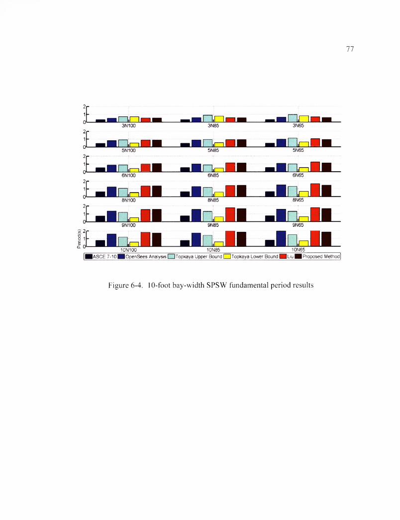
Perio
d(s)
77
DM m l1GN100 10N85 10N65
|ASCE 7~10MQpenSees Analysis I iTopkaya Upper Bound | iTopkaya Lower Bound 1HLiu H i Proposed Method]
Figure 6-4. 10-foot bay-width SPSW fundamental period results

Perio
d (s)
Pe
riod
(s)
78
5M100
. n M I6M100
l.i—i M l8M100
l£=L9M100
HI
l£ n10M100
LM
.no3M85
□ M l5M85
£ n M J6M85
8M85
n9M85
□ i
j it—ii3M65
n i l5M65
L t m6M65
8M65
9M65
£ H10M85
I «■10MW65
|ASCE 7-10 WM OpenSees Analysis! iTopkaya Upper Bound I iTopkaya Lower Bound M L iu M i Proposed Method]
Figure 6-5. 15-foot bay-width SPSW fundamental period results
10W100
1f -.1 I h m b
u
J —
3 W 1 0 0 3VV85
n n i5V\
J — -
m o o
, r n n « — ■
5VV85
■ r n n *
t m m
6V\MOO
n n i - ■
6VV85
a l AO' ' i
; f ■ ■
8V\im o o
n W M m M
8VV85
, n ( ! ■U *-------........... ........
L m *
9WMOO
n i l ■ !
9VV85
, n l ■10W85
a3W65
□ j5W65
o M j6W65
8W65
9W65n
Q10W65
0lASCE 7-10 B | OpenSees Analysis I ITopkaya Upper Bound □Topkaya Lower Bound B B t iu M Proposed Method]
Figure 6-6. 20-foot bay-width SPSW fundamental period results.

79
Table 6-6. 10-foot bay-width SPSW fundamental period results.
Fundamental Period Analysis Method
SPSWPrototype
ASCE 7- 10 (s)
Finite Element
Analysis (s)
Upper Bound: Topkaya's Method
‘ (s)
Lower Bound: Topkaya's Method
’ IS)
Liu'sMethod
(s)
Kean'sMethod
(s)3N100 0.499 0.700 0.669 0.512 0.526
3N85 0.312 0.566 0.883 0.768 0.571 0.553
3N65 0.618 0.953 0.788 0.661 0.557
5N100 0.807 0.880 0.495 0.861 0.870
5N85 0.458 0.854 0.940 0.532 0.907 0.913
5N65 0.952 1.080 0.608 1.017 0.919
6N100 0.860 0.870 0.437 0.993 1.040
6N85 0.525 0.993 0.884 0.477 1.133 1.092
6N65 1.045 0.997 0.533 1.237 1.098
8N100 1.245 1.085 0.522 1.358 1.380
8N85 0.651 1.303 1.183 0.563 1.420 1.449
8N65 1.491 1.293 0.673 1.657 1.456
9N100 1.334 1.192 0.510 1.515 1.550
9N85 0.711 1.521 1.269 0.580 1.734 1.627
9N65 1.543 1.269 0.580 1.745 1.634
10N100 1.583 1.203 0.555 1.799 1.719
10N85 0.770 1.722 1.405 0.563 1.972 1.804
10N65 1.940 1.475 0.686 2.176 1.811

80
Table 6-7. 15-foot bay-width SPSW fundamental period results.
Fundamental Period Analysis Method
SPSWPrototype
ASCE 7-10 (s)
FiniteElementAnalysis
(s)
Upper Bound: Topkaya's Method
(s)
Lower Bound: Topkaya's Method
' ( s )
Liu'sMethod
(s)
Kean'sMethod
(s)3M100 0.469 0.953 0.944 0.518 0.479
3M85 0.312 0.512 1.018 0.782 0.573 0.504
3M65 0.564 1.100 0.806 0.667 0.510
5M100 0.710 1.053 0.611 0.832 0.761
5M85 0.458 0.753 1.200 0.685 0.887 0.804
5M65 0.872 1.391 0.744 1.023 0.817
6M100 0.812 1.141 0.644 0.960 0.898
6M85 0.525 0.895 1.281 0.704 1.065 0.950
6M65 0.957 1.408 0.763 1.139 0.966
8M100 1.124 1.366 0.664 1.278 1.166
8M85 0.651 1.171 1.440 0.701 1.332 1.236
8M65 1.332 1.647 0.808 1.530 1.259
9M100 1.146 1.423 0.643 1.296 1.297
9M85 0.711 1.200 1.514 0.712 1.331 1.376
9M65 1.429 1.772 0.816 1.641 1.404
10M100 1.378 1.295 0.604 1.555 1.427
10M85 0.770 1.473 1.645 0.715 1.664 1.516
10M65 1.675 1.597 0.734 1.904 1.547

81
Table 6-8. 20-foot bay-width SPSW fundamental period results.
Fundamental Period Analysis Method
SPSWPrototype
ASCE 7-10 (s)
FiniteElementAnalysis
(s)Upper Bound:
Topkaya's Method (s)
Lower Bound: Topkaya's Method (s)
Liu'sMethod
(s)
Kean'sMethod
(s)3W100 0.442 1.083 0.739 0.499 0.454
3W85 0.312 0.490 1.207 0.813 0.554 0.477
3W65 0.536 1.347 0.919 0.602 0.483
5W100 0.645 1.285 0.739 0.790 0.703
5W85 0.458 0.688 1.440 0.774 0.822 0.744
5W65 0.771 1.582 0.839 1.108 0.758
6W100 0.737 1.307 0.748 0.922 0.821
6W85 0.525 0.788 1.493 0.783 0.979 0.871
6W65 0.911 1.725 0.927 1.151 0.890
8W100 0.895 1.236 0.611 1.081 1.051
8W85 0.651 1.016 1.316 0.681 1.237 1.119
8W65 1.085 1.529 0.739 1.315 1.147
9W100 1.028 1.625 0.780 1.169 1.163
9W85 0.711 1.127 1.729 0.819 1.253 1.239
9W65 1.228 2.027 0.928 1.355 1.273
10W100 1.214 1.478 0.671 1.402 1.273
10W85 0.770 1.344 1.496 0.685 1.562 1.358
10W65 1.521 1.547 0.714 1.759 1.397

82
CHAPTER 7. CONCLUSIONS
This study proposes a simplified method for approximating the fundamental period of a
SPSW structure. Fifty-four SPSW were designed in accordance to specifications outlined
in AISC Design Guide 20 [1], ASCE 7-10 [3], and AISC 341-10 [10], Using the finite
element analysis software OpenSees [21] finite element models were created for each
SPSW prototype and their fundamental period was calculated using an Eigen value
approach. A statistical analysis of the SPSW fundamental period data was performed using
MATLAB [26]. Using the results from the statistical analysis a method was developed
which adjusted the fundamental period coefficients used in ASCE 7-10 equation 12.8-7
based on the structures bay-width and base-shear participation ratios.
The proposed method was applied to the SPSW prototypes developed for this study
and could closely approximate the fundamental period when compared to a finite element
analysis. Three validation prototypes were then developed with story heights, bay-widths,
and base-shear participation ratios not considered in the initial SPSW population. The
proposed method was then used to approximate the fundamental period o f the validation
prototypes and compared with the finite element analysis. From the comparison, it was
found that the proposed method could closely approximate the fundamental period of the
validation SPSWs.
Based on the results from this study it can be stated that the proposed method can
approximate the fundamental period of a SPSW if designed similarly to the prototypes in
this method. The method proposed in this study is limited to the type of web-plate used in
the SPSW design. The prototypes developed for this study were all unstiffened and
unperforated steel web-plates. Further on the effects o f using web-plates with eccentric
configurations could expand the range where this method is valid.

83
References
[1] Sabelli, Rafael, S.E., and Michel Bruneau, Ph.D. "Steel Plate Shear Walls." Steel
Design Guide 20 Steel Plate Shear Walls. 2012 ed. Chicago: American Institute of Steel
Construction, 2007. Print.
[2] Seilie, Ignasius F., P.E., and John D. Hooper, P.E. "Steel Plate Shear Walls: Practical
Design and Construction." Modern Steel Construction (2005): n. pag. Web.
[3] Minimum Design Loads for Buildings and Other Structures. Reston, VA: American
Society of Civil Engineers, 2010. Print.
[4] Bruneau, Michel, Jeffrey W. Berman, Diego Lopez-Garcia, and Darren Vian. "A
Review of Steel Plate Shear Wall Design Requirements and Research." Engineering
Journal (2007): 27-34. Web
[5] Elgaaly, M., V. Caccese, and C. Du. "Postbuckling Behavior of Steel-Plate Shear
Walls under Cyclic Loads." Journal o f Structural Engineering J. Struct. Eng. 119.2
(1993): 588-605. Web.
[6] Caccese, Vincent, Mohamed Elgaaly, and Ruobo Chen. "Experimental Study of Thin
Steel-Plate Shear Walls under Cyclic Load." Journal o f Structural Engineering J. Struct.
Eng. 119.2 (1993): 573-87. Web.
[7] Lubell, Adam S., Helmut G. L. Prion, Carlos E. Ventura, and Mahmoud Rezai.
"Unstiffened Steel Plate Shear Wall Performance under Cyclic Loading." Journal o f
Structural Engineering J. Struct. Eng. 126.4 (2000): 453-60. Web.

84
[8] Enright, James Thomas. Improving Steel Plate Shear Wall Code Design
Methodology. Thesis. San Francisco State University, 2014. N.p.: n.p., n.d. Print.
[9] Barghi, Ramin David. Evaluation of Maximum Likelihood Fitting for Fragility
Analysis of Code-Designed Steel Plate Shear Walsl. Thesis. San Francisco State
University, 2015. N.p.: n.p., n.d. Print.
[10] Seismic Provisions for Structural Steel Buildings. Chicago, IL: American Institute of
Steel Construction, 2010. Print.
[11] Liu, Shi, Gordon P. Warn, and Jeffrey W. Berman. "Estimating Natural Periods of
Steel Plate Shear Wall Frames." Journal of Structural Engineering J. Struct. Eng. 139.1
(2013): 155-61. Web.
[12] Berman, Jeffrey W. "Seismic Behavior of Code Designed Steel Plate Shear
Walls." Seismic Behavior of Code Designed Steel Plate Shear Walls. Engineering
Structures, 9 Nov. 2010. Web.
[13] Topkaya, Cem, and Can Ozan Kurban. "Natural Periods of Steel Plate Shear Wall
Systems." Journal of Constructional Steel Research 65.3 (2009): 542-51. Web.
[14] Zalka, K.a. "A Simplified Method for Calculation of the Natural Frequencies of
Wall-frame Buildings." Engineering Structures 23.12 (2001): 1544-555. Web.
[15] Atasoy, M. Lateral Stiffness o f Unstiffened Steel Plate Shear Walls. Thesis. Middle
East Technical University, 2008. N.p.: n.p., n.d. Print.
[16] Gupta, A., and Krawinkler, H. (1999). "Seismic Demands for Performance
Evaluation of Steel Moment Resisting Frame Structures," Technical Report 132,
The John A. Blume Earthquake Engineering Research Center, Department of Civil
Engineering, Stanford University, Stanford, CA.

85
[17] Dunkerley, S. On the Whirling and Vibration o f Shafts. London: Harrison and Sons,
1894. Print.
[18] Chopra, Anil K. Dynamics of Structures: Theory and Applications to Earthquake
Engineering. Englewood Cliffs, NJ: Prentice Hall, 1995. Print.
[ 19] BENDING FREQUENCIES OF BEAMS, RODS, AND PIPES Revision S By Tom
Irvine Email: [email protected] November 20, 2012 (n.d.): n. pag. Web.
[20] Topkaya, Cem, and Mehmet Atasoy. "Lateral Stiffness of Steel Plate Shear Wall
Systems." Thin-Walled Structures 47.8-9 (2009): 827-35. Web.
[21] "Open System for Earthquake Engineering Simulation - Home Page." Open System
for Earthquake Engineering Simulation - Home Page. N.p., n.d. Web.
[22] "Eigen Command." - OpenSeesWiki. N.p., n.d. Web.
<http://opensees.berkeley.edu/wiki/index.php/Eigen_Command>.
[23] "Main Page." OpenSeesWiki. N.p., n.d. Web.
<http://opensees.berkeley.edu/wiki/index.php/Main_Page>.
[24] "ElemPanelZone2D.tcl." - OpenSeesWiki. N.p., n.d. Web.
<http://opensees.berkeley.edu/wiki/index.php/ElemPanelZone2D.tcl>.
[25] Eads, Laura. "Pushover and Dynamic Analysis of 2 Story Moment
Frame."OpenSees Wiki. U.C. Berkeley, n.d. Web.
<http://opensees.berkeley.edu/wiki/index.php/Pushover_and_Dynamie_Analyses_of_2-
Story_Moment_Frame_with_Panel_Zones_and_RBS>.
[26] "Documentation." MATLAB. Mathworks, n.d. Web.
<http://www.mathworks.com/help/matlab/>.
[27] "Documentation." Power Series. Mathworks, n.d. Web.
<http://www.mathworks.com/help/curvefit/power.html>.

86
[28] "Documentation." Linear Regression. Mathworks, n.d. Web. 19 Dec. 2015.
<http://www.mathworks.com/help/matlab/data_analysis/linear-regression.html>.
[29] "Documentation." Root-mean-square Level. Web. 19 Mar. 2016.
<http://www.mathworks.com/help/signal/ref/rms.html?s_tid=gn_loc_drop>.
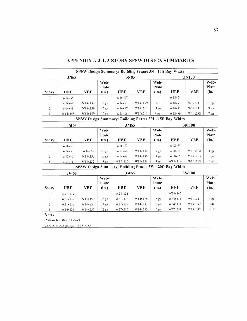
87
APPENDIX A-2-1. 3-STORY SPSW DESIGN SUMMARIES
SPSW Design Summary: Building Frame 3N - 10ft Bay-Width3N65 3N85 3N100
Story HBE VBE
Web-Plate(in.) HBE VBE
Web-Plate(in.) HBE VBE
Web-Plate(in.)
R W 18x65 - - W 16x57 - - W18x71 - -
3 W 14x48 W14xl32 18 ga W16x57 W14xl59 1/16 W18x71 W14x211 13 ga
2 W 14x48 W14xl59 13 ga W 16x57 W14x211 11 ga W 18x71 W 14x211 9 ga
1 W14xl58 W14xl59 12 ga W 18x86 W14x211 9 ga W 18x86 W 14x283 7 ga
SPSW Design Summary: Building Frame 3M - 15ft Bay-Width
3M65 3M85 3M100
Story HBE VBE
Web-Plate(in.) HBE VBE
Web-Plate(in.) HBE VBE
Web-Plate(in.)
R W16x57 - - W 16x77 - - W 18x65 - -
3 W 16x57 W 14x74 20 ga W 14x68 W14xl32 19 ga W 18x71 W14xl32 18 ga
2 W 12x45 W14xl32 16 ga W 14x48 W14xl45 14 ga W 18x65 W14xl93 13 ga
1 W 18x86 W14xl32 15 ga W18xl 19 W14xl45 13 ga W18xl 19 W14xl93 12 ga
SPSW Design Summary: Building Frame 3W - 20ft Bay-Width
3W65 3W85 3W100
Story HBE VBE
Web-Plate(in.) HBE VBE
Web-Plate(in.) HBE VBE
Web-Plate(in.)
R W21xl32 - - W24xl31 - - W24xl62 - -
3 W21xl32 W14xl59 18 ga W21xl22 W14xl76 16 ga W24xl31 W14x211 14 ga
2 W21xl32 W 14x257 13 ga W21xl22 W 14x283 12 ga W24xl31 W 14x342 1/81 W24x229 W 14x257 12 ga W27x217 W 14x283 10 ga W27x281 W 14x342 3/16
NotesR denotes Roof Level ga deontoes gauge thickness

88
APPENDIX 2-2-2. 5-STORY SPSW DESIGN SUMMARIES
SPSW Design Summary: Building Frame 5N - 10ft Bay-Width5N65 5N85 5N100
Story HBE VBE
Web-Plate(in.) HBE VBE
Web-Plate(in.) HBE VBE
Web-Plate(in.)
R W 14x68 - W 14x68 - - W 12x50 - -
5 W 14x68 W 14x82 22 ga W 14x68 W14xl32 20 ga W12x50 W14xl59 18 ga
4 W 14x68 W14xl32 17 ga W 14x68 W14xl32 14 ga W12x50 W14xl59 13 ga
3 W 14x68 W14xl32 14 ga W 14x68 W14xl59 12 ga W12x50 W14xl59 11 ga
2 W 14x68 W14xl93 13 ga W 14x68 W 14x233 11 ga W 12x50 W14x211 9 ga
1 W 14x68 W14xl93 12 ga W 14x74 W 14x233 10 ga W 12x96 W14x257 8 ga
SPSW Design Summary: Building Frame 5M - 15ft Bay-Width5M65 5M85 5M100
Story HBE VBE
Web-Plate(in.) HBE VBE
Web-Plate(in.) HBE VBE
Web-Plate(in.)
R W 14x53 - - W 14x68 - - W 18x65 - -
5 W 14x53 W 14x74 24 ga W 14x68 W 14x82 21 ga W 18x65 W14xl32 19 ga
4 W 14x48 W14xl32 18 ga W 14x68 W14xl45 16 ga W 18x65 W14xl32 14 ga
3 W 14x48 W14xl32 15 ga W 14x68 W14xl45 13 ga W 14x74 W14xl93 12 ga
2 W 14x53 W14xl32 14 ga W 14x68 W14x211 12 ga W 14x74 W14xl93 11 ga
1 W14x257 W14xl59 13 ga W30x211 W14x211 12 ga W24xl92 W 14x233 10 ga
SPSW Design Summary: Building Frame 5W - 20ft Bay-Width5W65 5W85 5W100
Story HBE VBE
Web-Plate(in.) HBE VBE
Web-Plate(in.) HBE VBE
Web-Plate(in.)
R W 18x97 - - W21xl 11 - - W21xl22 - -
5 W 18x86 W14xl32 23 ga W14xl59 W14xl32 21 ga W21xl32 W14xl45 19 ga
4 W16x77 W14xl32 17 ga W14xl93 W14xl76 15 ga W 16x77 W14x211 13 ga
3 W 16x77 W14xl45 15 ga W 16x77 W14x211 13 ga W 18x97 W14xl93 12 ga
2 W 14x48 W14xl76 13 ga W 16x77 W14xl93 12 ga W21xl 11 W14x257 10 ga
1 W30x211 W14xl76 13 ga W27x217 W 14x370 11 ga W33x236 W14x311 10 ga
NotesR denotes Roof Level ga deontoes gauge thickness

89
APPENDIX A-2-3. 6-STORY SPSW DESIGN SUMMARIES
SPSW Design Summary: Building Frame 6N - 10ft Bay-Width6N65 6N85 6N100
Story HBE VBE
Web-Plate( in .) HBE VBE
Web-Plate(in.) HBE VBE
Web-Plate(in.)
R W 18x65 - W21x93 - - W21x93 - -
6 W16x57 W14xl45 19 ga W16x57 W14xl76 17 ga W 18x65 W14x257 16 ga
5 W 14x48 W14xl45 13 ga W16x57 W14xl76 12 ga W 16x57 W14x257 11 ga
4 W 14x48 W 14x233 11 ga W16x57 W 14x257 9 ga W16x57 W 14x342 7 ga
3 W 14x48 W14x233 10 ga W 16x57 W 14x257 7 ga W 18x65 W 14x342 5 ga
2 W 14x48 W14x311 9 ga W18x65 W14x370 5 ga W 18x65 W14x455 3 ga
1 W 14x86 W14x311 8 ga W21x93 W14x370 5 ga W21xl 11 W 14x455 1/4
SPSW Design Summary: Building Frame 6M - 15ft Bay-Width6M65 6M85 6M100
Story HBE VBE
Web-Plate(in.) HBE VBE
Web-Plate(in.) HBE VBE
Web-Plate(in.)
R W16x57 - W16x57 - - W 18x65 - -
6 W16x57 W14xl32 23 ga W16x57 W14xl45 21 ga W 18x65 W14xl76 19 ga
5 W16x57 W14xl32 18 ga W 16x57 W14xl45 1/16 W 18x65 W14xl76 14 ga
4 W 16x57 W14xl32 15 ga W 16x57 W14xl45 13 ga W 18x65 W14xl76 12 ga
3 W 16x57 W 14x211 13 ga W16x57 W 14x233 12 ga W 18x65 W 14x283 1/82 W16x57 W14x211 12 ga W16x57 W14x233 11 ga W 18x65 W 14x283 9 ga
1 W18xl 19 W14x211 12 ga W21x211 W 14x233 1/8 W21xl32 W 14x283 9 ga

90
SPSW Design Summary: Building Frame 6W - 20ft Bay-Width6W65 6W85 6W100
Story HBE VBE
Web-Plate(in.) HBE VBE
Web-Plate(in.) HBE VBE
Web-Plate(in.)
R W18xl06 - - W24xl31 - - W21xl32 - -
6 W18xl06 W14xl32 23 ga W21xl 11 W14xl93 20 ga W21xl32 W 14x211 19 ga
5 W18xl06 W14xl32 17 ga W21x93 W14xl93 14 ga W21xl32 W14x211 13 ga
4 W 18x65 W14xl76 14 ga W 16x77 W14x233 12 ga W16x77 W 14x257 11 ga3 W 18x65 W14xl76 13 ga W 16x77 W14x233 11 ga W 16x77 W 14x257 10 ga
2 W18x65 W 14x233 12 ga W 16x77 W14x311 10 ga W 16x77 W14x342 9 ga
1 W24x229 W 14x233 12 ga W30x211 W14x311 9 ga W30x235 W 14x342 8 ga
NotesR denotes Roof Level ga deontoes gauge thickness

91
APPENDIX A-2-4. 8-STORY SPSW DESIGN SUMMARIES
SPSW Design Summary: Building Frame 8N - 10ft Bay-Width8N65 8N85 8N100
Story HBE VBE
Web-Plate(in.) HBE VBE
Web-Plate(in.) HBE VBE
Web-Plate(in.)
R W 14x68 - W 14x82 - - W 14x68 - -
8 W 14x68 W14xl59 21 ga W 14x82 W14xl45 19 ga W 14x82 W14x211 18 ga
7 W 14x68 W14xl59 15 ga W 14x82 W14xl45 13 ga W 14x68 W14x211 12 ga
6 W 14x68 W14xl59 13 ga W 14x68 W14x370 11 ga W 14x68 W14x211 9 ga
5 W 14x68 W 14x283 11 ga W 14x68 W 14x370 9 ga W 14x68 W14x455 7 ga
4 W 14x68 W 14x283 10 ga W14xl32 W14x370 7 ga W 14x68 W 14x455 5 ga
3 W 16x89 W 14x289 9 ga W14xl32 W14x370 6 ga W 14x68 W 14x455 3 ga
2 W 16x89 W 14x370 9 ga W14xl32 W 14x500 5 ga W14x68 W14x455 1/4
1 W 16x89 W14x370 8 ga W16xl00 W 14x500 5 ga W14xl32 W14x550 1/4
SPSW Design Summary: Building Frame 8M - 15ft Bay-Width8M65 8M85 8M100
Story HBE VBE
Web-Plate(in.) HBE VBE
Web-Plate(in.) HBE VBE
Web-Plate(in.)
R W 14x68 - - W 14x74 - - W 14x82 - -
8 W 14x68 W14xl32 24 ga W 14x82 W14xl59 20 ga W 14x82 W14xl76 22 ga
7 W 14x68 W14xl32 18 ga W 14x68 W14xl59 14 ga W 14x82 W14xl76 16 ga
6 W 14x68 W14xl32 16 ga W 14x68 W14xl59 12 ga W 14x53 W14xl76 13 ga
5 W 14x68 W14xl93 14 ga W 14x68 W14x342 10 ga W 14x82 W14xl76 12 ga
4 W 14x68 W14xl93 13 ga W 14x68 W 14x342 9 ga W 14x48 W14x283 10 ga
3 W 14x68 W14xl93 13 ga W 14x68 W14x342 8 ga W 14x48 W14x283 10 ga
2 W 14x68 W14x257 12 ga W21xl 11 W 14x342 7 ga W 14x48 W14x283 9 ga
1 W 18x86 W 14x257 12 ga W30x235 W14x426 7 ga W21xl22 W14x342 9 ga

92
SPSW Design Summary: Building Frame 8W - 20ft Bay-Width8W65 8W85 8W100
Story HBE VBE
Web- Plate
....(in.).... HBE VBE
Web-Plate(in.) HBE VBE
Web-Plate(in.)
R W18xl 19 - W21xl22 - W18xl92 -
8 W 18xl 19 W14x211 22 ga W21xl 11 W 14x233 19 ga W18xl92 W l 4x257 18 ga
7 W18xl 19 W14x211 16 ga W24xl31 W 14x233 14 ga W18xl58 W14x257 12 ga
6 W14xl32 W14x211 13 ga W24xl31 W14x283 11 ga W 18xl 19 W 14x426 9 ga
5 W14xl32 W 14x342 12 ga W 18x86 W14x283 9 ga W18xl 19 W 14x426 8 ga
4 W 18x86 W14x342 11 ga W18x86 W 14x426 8 ga W18xl75 W 14x426 6 ga
3 W14xl32 W 14x342 10 ga W18x86 W 14x426 7 ga W18x97 W 14x426 5 ga
2 W24x306 W 14x342 9 ga W 18x86 W 14x426 3/16 W27x368 W 14x500 4 ga
1 W24x306 W14x500 9 ga W33x221 W14x426 6 ga W27x668 W l 4x730 4 ga
NotesR denotes Roof Levelga deontoes gauge thickness

93
APPENDIX A-2-5. 9-STORY SPSW DESIGN SUMMARIES
SPSW Design Summary: Building Frame 9N - 10ft Bay-Width9N65 9N85 9N100
Story HBE VBE
Web-Plate( in .) HBE VBE
Web-Plate(in.) HBE VBE
Web-Plate(in.)
R W21x93 - W 12x50 - - W16x77 -
9 W 14x48 W14xl59 21 ga W12x50 W14xl59 19 ga W16x77 W14xl76 18 ga
8 W 14x48 W14xl59 15 ga W12x50 W14xl59 13 ga W 16x77 W14xl76 12 ga
7 W21x93 W14xl59 13 ga W16x57 W14xl59 11 ga W 16x77 W14x311 9 ga
6 W21x93 W 14x342 11 ga W16x57 W 14x342 9 ga W16x77 W14x311 6 ga
5 W 14x48 W 14x342 9 ga W16x57 W 14x342 7 ga W16x77 W 14x455 3 ga
4 W 14x48 W 14x342 8 ga W16x57 W 14x342 5 ga W16x77 W14x455 1/4
3 W21x93 W14x550 7 ga W16x57 W14x550 4 ga W 16x77 W14x730 5/16
2 W21x93 W14x550 3/16 W16x57 W14x550 4 ga W 16x77 W14x730 5/16
1 W 14x90 W14x550 3/16 W 18x97 W14x550 3 ga W18xl30 W14x730 5/16
SPSW Design Summary: Building Frame 9M - 15ft Bay-Width9M65 9M85 9M100
Story HBE VBE
Web-Plate(in.) HBE VBE
Web-Plate(in.) HBE VBE
Web-Plate(in.)
R W16x57 - - W21x93 - - W 16x77 - -
9 W16x57 W14xl32 23 ga W 18x65 W14x211 20 ga W 16x77 W14x211 19 ga
8 W16x57 W14xl32 17 ga W 18x65 W14x211 15 ga W16x77 W 14x211 13 ga
7 W16x57 W14xl32 14 ga W21x93 W14x211 12 ga W 16x77 W 14x211 1/86 W16x57 W14x283 12 ga W 18x65 W 14x455 10 ga W16x77 W 14x426 8 ga
5 W16x57 W14x283 11 ga W 18x65 W 14x455 9 ga W 16x77 W 14x426 6 ga
4 W 16x57 W14x283 10 ga W21x93 W14x455 8 ga W16x77 W 14x426 5 ga
3 W 16x57 W 14x426 10 ga W 18x65 W 14x605 7 ga W 16x77 W 14x665 4 ga
2 W16x57 W 14x426 9 ga W 18x65 W 14x605 6 ga W16x77 W 14x665 3 ga
1 W18xl75 W 14x426 9 ga W33x241 W 14x605 6 ga W24xl92 W 14x665 1/4

94
SPSW Design Summary: Building Frame 9W - 20ft Bay-Width9W65 9W85 9W100
Story HBE VBE
Web-Plate(in.) HBE VBE
Web-Plate(in.) HBE VBE
Web-Plate(in.)
R W21x93 - W21xl32 - - W21xl32 - -
9 W21x93 W14xl76 22 ga W21xl32 W 14x233 19 ga W21xl22 W14x257 18 ga
8 W21x93 W14xl76 16 ga W21x93 W 14x233 13 ga W21xl22 W 14x257 13 ga
7 W21x93 W14xl76 13 ga W21x93 W l 4x233 11 ga W21xl22 W 14x257 10 ga
6 W 18x97 W 14x455 11 ga W21x93 W 14x500 9 ga W21xl22 W l 4x605 7 ga
5 W 18x97 W l 4x455 1/8 W21x93 W 14x500 7 ga W21x93 W 14x605 5 ga
4 W18x86 W14x550 9 ga W21x93 W l 4x500 3/16 W21x93 W 14x605 4 ga
3 W 18x86 W 14x605 9 ga W21x93 W 14x665 5 ga W21x93 W14x730 3 ga
2 W18x86 W 14x605 8 ga W21x93 W 14x665 4 ga W21x93 W 14x730 1/4
1 W24x335 W 14x605 ....8 £a.... W33x263 W 14x665 4 ga W30x326 W l 4x730 1/4
NotesR denotes Roof Levelga deontoes gauge thickness

95
APPENDIX A-2-6. lO-STORY SPSW DESIGN SUMMARIES
SPSW Design Summary: Building Frame ION - 10ft Bay-Width10N65 10N85 10N100
Story HBE VBE
Web-Plate(in.) HBE VBE
Web-Plate
......<>"•) ....._ HBE VBE
Web-Plate(in.)
R W 14x48 - - W 14x48 - W 16x77 - -
10 W 14x48 W14xl76 21 ga W14x53 W14xl32 19 ga W 16x77 W14x211 17 ga
9 W 14x48 W14xl76 15 ga W 14x48 W14xl32 13 ga W 16x77 W14x211 12 ga
8 W14x48 W14xl76 12 ga W 14x48 W 14x283 10 ga W16x77 W 14x211 9 ga
7 W 14x48 W14xl76 11 ga W14x53 W 14x283 8 ga W 16x77 W14x398 3/16
6 W14xl32 W 14x426 9 ga W 14x48 W14x550 6 ga W16x77 W l 4x398 4 ga
5 W14xl32 W 14x426 8 ga W14x68 W14x550 5 ga W 16x77 W14x398 1/4
4 W14xl32 W 14x426 7 ga W 14x68 W14x550 3 ga W 16x77 W14x730 5/16
3 W 14x82 W 14x426 7 ga W 14x48 W14x550 1/4 W 16x77 W l 4x730 5/16
2 W14x82 W 14x426 6 ga W 14x48 W l 4x550 5/16 W 16x77 W 14x730 5/16
1 W14xl32 W l 4x500 6 ga W14xl59 W 14x665 5/16 W14xl59 W14x730 5/16
SPSW Design Summary: Building Frame 10M - 15ft Bay-Width10M65 10M85 10M100
Story HBE VBE
Web-Plate(in.) HBE VBE
Web-Plate(in.) HBE VBE
Web-Plate(in.)
R W 14x74 - - W 16x57 - - W16x77 - -
10 W 14x74 W14xl76 23 ga W 16x77 W14xl32 20 ga W16x77 W 14x257 19 ga
9 W 14x74 W14xl76 17 ga W 16x77 W14xl32 14 ga W 14x68 W l 4x257 13 ga
8 W14x53 W14xl76 13 ga W16x77 W 14x342 12 ga W 18x86 W14x257 11 ga
7 W14x53 W14xl76 12 ga W 16x77 W 14x342 10 ga W 16x77 W l 4x257 8 ga
6 W16x57 W 14x342 11 ga W 16x77 W 14x342 8 ga W 14x82 W 14x500 6 ga
5 W 14x68 W 14x342 10 ga W 16x77 W 14x342 7 ga W 14x74 W 14x500 5 ga
4 W 14x48 W 14x342 9 ga W 16x77 W14x550 6 ga W 14x74 W l 4x500 4 ga
3 W14xl32 W 14x342 9 ga W 14x82 W14x550 5 ga W18x86 W 14x500 3 ga
2 W14xl32 W 14x455 8 ga W 14x82 W14x550 5 ga W14xl32 W 14x665 1/4
1 W l 4x370 W l 4x455 8 ga W24xl46 W14x550 5 ga W40x264 W 14x665 1/4

96
SPSW Design Summary: Building Frame 10W - 20ft Bay-Width10W65 10W85 10W100
Story HBE VBE
Web-Plate
HBE VBE
Web-Plate(in.) HBE VBE
Web-Plate(in.)
R W18xl 19 -
.....W21xl22 - - W l 8x234 - -
10 W18xl 19 W14xl59 22 ga W24xl31 W 14x233 19 ga W18xl58 W 14x283 18 ga
9 W18xl 19 W14xl59 16 ga W21xl 11 W 14x233 13 ga W18xl58 W 14x283 13 ga
8 W18xl 19 W14x257 13 ga W21xl 11 W l 4x233 11 ga W18xl58 W 14x283 10 ga
7 W18xl 19 W 14x283 11 ga W 18x86 W l 4x283 9 ga W18xl58 W 14x455 8 ga
6 W18xl 19 W l 4x283 10 ga W21xl 11 W 14x500 8 ga W18xl58 W l 4x455 6 ga
5 W 16x89 W l 4x455 9 ga W21xl22 W 14x500 6 ga W18xl58 W 14x455 4 ga
4 W 16x77 W14x455 8 ga W 18x97 W 14x500 5 ga W 18x234 W l 4x730 3 ga
3 W 16x89 W 14x455 8 ga W21xl22 W 14x500 4 ga W18xl58 W 14x730 5/16
2 W 16x77 W l 4x455 7 ga W21xl22 W 14x605 4 ga W18xl58 W14x730 5/16
1 W24x335 W 14x455 7 ga W40x278 W 14x605 4ga W27x537 W14x730 5/16
NotesR denotes Roof Levelga deontoes gauge thickness

97
APPENDIX A-3-1. LIU E T A L . SPSW FUNDAMENTAL PERIOD
APPROXIMATION METHOD
Liu et al. SPSW Fundamental Period Approximation Method
SPSW Prototype: 5W85
Input:Percentage of Shear in Pate
Building Information
Number of Stoires:
Levels:
Frame Width:
k := 0 .8 f
n := 5
i := 0 .. n - 1
Length := 24( L* := Length-in
LT = (240 240 240 240 2 4 0 )-in
Frame Height:
Unbraced Length:
Height := 15f
T
h := Height in-(1 1 1 1 1 1 )
h * = (13 13 13 13 13 13) ft
H :=AW
^6- 156-in >
oor-
5-156-in 65
4-156-in 52
3-156-in 39
2-156-in 26
v 156-in J ,13 J
• f t
Lb := — 3
Lb =(6.667 6.667 6.667 6.667 6.667)ft
Number of Shear Walls on a Story: Nsh := 4
Dead Load: Po l ^ 96 96 96 % % > V f
Live Load: pLL:= lOOpsf

98
Seismic Design sDS := 1.0'Acceleration:
Sds := 1.0'
Sdl := 0.7S
Material Properties
Web Plate
Steel Web Yield Strength:
Ratio of expected yield stress to the minimum yield stress:
Boundary ElementsSteel Yield Strength:
Ration of expected yield stress to the minimum yield stress:
Steel Modulus of Elasticity:
Fyweb := 36'ksi
Ryw :=l-2
Fy := 50ksi
:= 1.1
E := 29000ksi
Effective Length factor:
CodeBending phi factor
Tension phi factor
Shear phi factor
Compression phi factor
K := l.CAAAA
* b := 0.S
<j,t := O.S
<t>v := 1C
d»c := O.S
Braced member phi factor := 0.7f
ASTM A36
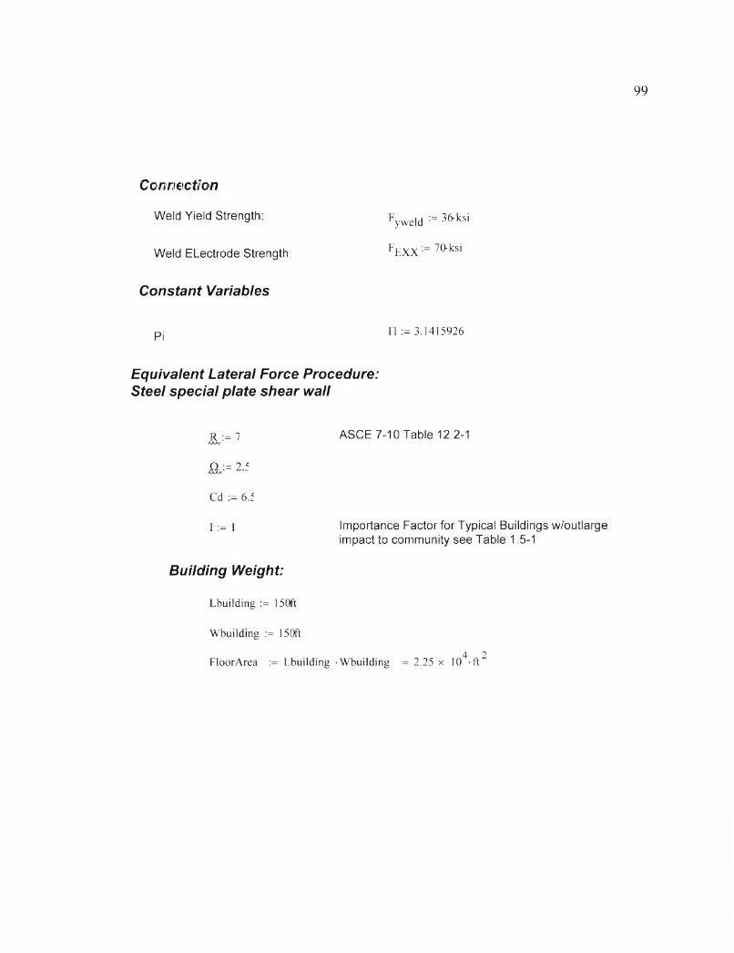
99
Connection
Weld Yield Strength: FyWeld := 36 ksi
Weld ELectrode Strength: FEXX:= 70 ksi
Constant Variables
P I n := 3.1415926
Equivalent Lateral Force Procedure: Steel special plate shear wall
r := 7 ASCE 7-10 Table 12.2-1AAA/
Q := 2 .fAAAA
Cd := 6.5
I := i Importance Factor for Typical Buildings w/outlargeimpact to community see Table 1.5-1
Building Weight:
Lbuilding := 150ft
Wbuilding := 150ft
4 2FloorArea := Lbuilding Wbuilding = 2.25 x 10 ft

100
Wh. := p ^ L ’FloorArea
Wh =
1.867x 10
2.16x 10
2.16x 10
2.16x 10
2.16x 10
kip
FlrW := stack(w h0 ,W hr Wh2 ,W h3 ,W h4j
FlrW
1.867x 10
2.16x 10
2.16x 10
2.16x 10
kip
2.16x 10 J
W := Y FlrW. = 1.051 x 10⁴-kip/WW / , 1 ri
WEB PLATE DESIGN PROPERTIES
Standard Steel Plate Thicknesses
wSTD '1 3 1 5 3 7 1 9 5 Y 1
- ins j _1 16 8 16 4 16 8 16 2 16

101
Gauge Steel Defined
wg •
0
0
0
0.2391
0.2242
0.2092
0.1943
0.1793
0.1644
0.1495
0.1345
0.1198
0.1046
0.0897
0.0747
0.0673
0.0598
0.0538
0.0478
0.0418
0.0359
0.0329
0.0299
0.0269
v0.0239y
in
Steel Gauge begins at 3
Web Plate Thickness Per Story
V :=
•wg21
^0.0027^'wSl5 0.0056
wSi3 = 0.0075
0.0087w®12 v 0.01 j
W lly
fit
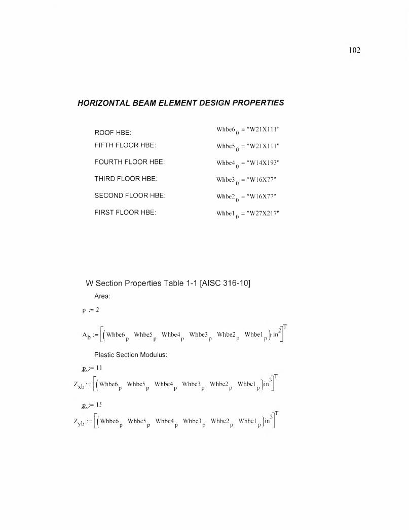
HORIZONTAL BEAM ELEMENT DESIGN PROPERTIES
ROOF HBE:
FIFTH FLOOR HBE:
FOURTH FLOOR HBE:
THIRD FLOOR HBE:
SECOND FLOOR HBE:
FIRST FLOOR HBE:
Whbe6 Q = "W21X111"
Whbe5Q = "W21X111"
Whbe4Q = "W14X193"
Whbe3Q = "W16X77"
Whbe2 Q = "W16X77"
Whbel Q = "W27X217"
W Section Properties Table 1-1 [AISC 316-10]Area:
p := 2
. 2' Whbe6 Whbe5 Whbe4 Whbe3 Whbe2 Whbel in I P P P P P P
Plastic Section Modulus:
Lxb '=. 3Whbe6 Whbe5 Whbe4 Whbe3 Whbe2 Whbel in
I P P P P P P
Zyb :_. 3
Whbe6 Whbe5 Whbe4 Whbe3 Whbe2 Whbel in I p P P P P P

103
Inertial Properties:
v := 1CHAKi
4Iu := ( Whbe6 Whbe5 Whbe4 Whbe3 Whbe2 Whbel )mb LA P P P P P P /
J L := 3
du:=f('w hbe6 Whbe5 Whbe4 Whbe3 Whbe2 Whbel jinj1b LA P P P P P P / J
S U = 17
r , ;= [YWhbe6 Whbe5 Whbe4 Whbe3 Whbe2 Whbel W"IT y t > L v P P P P P P / J
13r , := [YWhbe6 Whbe5 Whbe4 Whbe3 Whbe2 Whbel )in“|TxD LA P P P P P P / J
£L'-=4bfl, := |7Whbe6 Whbe5 Whbe4 Whbe3 Whbe2 Whbel )in“|T
™ Lv P P P P P Pt J
&,:= 6
tfh '■-[(Whbe6 Whbe5 Whbe4 Whbe3 Whbe2 Whbel )in1Ttb LI p p p p p p / J
JL--8htwu := (Ywhbe6 Whbe5 Whbe4 Whbe3 Whbe2 Whbel 'l'iT
b U P P P P P pJ J
£J= 5
t , := 7 Whbe6 Whbe5 Whbe4 Whbe3 Whbe2 Whbel l in fw b Lv p p p p p p / J
Plastic Development Length:
JL:= 9
L. := \ ( Whbe6 Whbe5 Whbe4 Whbe3 Whbe2 Whbel Vftli3 LV P P P P P P / J

104
10.24 > ^0.227 > f 1.208 N f 0.129 N
10.24 0.227 1.208 0.129
14.31 0.394 2 1.537 0.116ft A b = Z xb = gaI Jb =8.72 u 0.157 0.649 u 0.054
8.72 0.157 0.649 0.054
,11.73 , v 0.444 , v 3.078 j v 0.43 ,
f t
d b =
1.792 A
1.792
1.292
1.375
1.375
2.367 )
VERTICAL BOUNDARY ELEMENT DESIGN PROPERTIES
FIFTH FLOOR VBE: Wvbe50 = "W14X132’
FOURTH FLOOR VBE: Wvbe40 = "W14X176'
THIRD FLOOR VBE: Wvbe3Q = "W14X2111
SECOND FLOOR VBE: Wvbe2Q = "W14X193'
FIRST FLOOR VBE: Wvbel = "W14X370'
W Section Properties Table 1-1 [AISC 316-10]
Area:
Ac .
SJ-=2
(Wvbe5 Wvbe4 Wvbe3 Wvbe2 Wvbel P P P P PKf

105
Modulus of Plasticity:
&„■= 1 1
z •=xc •. 3f Wvbe5 Wvbe4 Wvbe3 Wvbe2 Wvbel W
{ P P P P P/
JL:=
zyc • Wvbe5 Wvbe4 Wvbe3 Wvbe2 Wvbel I P P P P
Inertial Properties:
d := 1C
!C := (Wvbe5 Wvbe4 Wvbe3 Wvbe2 Wvbel )in \ P P P P P/
£ .:= 3
dp := r(Wvbe5 Wvbe4 Wvbe3 Wvbe2 Wvbel )in1 c Ll P P P P P / J
i T
r :=f(Wvbe5 Wvbe4 Wvbe3 Wvbe2 Wvbel V I 1 yc LI P P P P P / J
13
■ iTr ;= [Y Wvbe5 Wvbe4 Wvbe3 Wvbe2 Wvbel \in~l xc LV P P P P P / J£L-=4
- [ (b^c := Wvbe5 Wvbe4 Wvbe3 Wvbe2 Wvbel • -|T
• nTtfP :=|7Wvbe5 Wvbe4 Wvbe3 Wvbe2 Wvbel W~|tc L\ p p p p p / J
htw. := ( Wvbe5 Wvbe4 Wvbe3 Wvbe2 Wvbel )T c \ p p p p p)
t_ := rfWvbe5 Wvbe4 Wvbe3 Wvbe2 Wvbel Vnlwc LI P P P P P / J

Plastic Development Length:
S c == [(Wvbe5 Wvbe4 Wvbe3 Wvbe2 Wvbel P P P P P
S c T =
r 13.28^
14.2
14.38
14.31
v 15.08y
).«]
V
0.269^
0.36
0.431
0.394
0.757y
f t 7 -xc
r 1.013n
1.385
1.688
1.537
v3.186y
gal L =
r 0.074^
0.103
0.128
0.116
v0.262y
dc =
r 1.225^
1.267
1.308
1.292
0 .4 9 2 ,
f t
Angle of Inclination
a . := atan i
1 +tw L.Wj i
2* A c-
1 + tw -h .■Wj i 360 L L. A h c. , b.
( 0.764 > 43.791 ^
0.75180
42.963
0.757 a deg a — - 43.352
0.723 41.401
v 0.716 j v41.016 j

alpha := reverse (a)
Length of beam from centerline: Lcf := L - d
Approximation MethodShear Frequency Calculation
Column Stiffness
1 2 E L
(hif
r 280.496^
392.328
487.66
439.994
v 997.32
kipin
/
Web Plate Stiffness
EL. t .i i:= “ ( h y (sin(alpbai)) -(cos(alphai))
Total Stiffness
1.311 x 10
1.148x 10³
997.192
746.864
v 366.309 j
kipin
k. := k„ +. + kp. = - 1 F1
/
Define Global Stiffness Matrix
1.591 x 10
1.541 x 10
1.485x 10
1.187 x 10
1.364 x 10 J

108
% + k3 " k3
-k3 k3 + k2
“ tot :=-k 2 k2 + kj
0
0 0
k l + k0 “ko
Define Mass Matrix
a := 32.2g
m. := 1
FlrW.
Nsh 'gm :
4.669 x 10
5.4 x 10
5.4 x 10
5.4 x 10
5.4 x 10
•lb
M := diag ( m4 m3 m2 m i m0 f
cos := J sort eigenvals M ' • JJ =
f 9.043 ^
27.595
42.628
53.528
v 62.66 j
Shear Natural Frequency of System
©c = 9.043— s0 s
2-nT •=----- = 0.695s
°°ss0

109
Flexure Frequency Calcualtion
Average mass
Z mi
Have • n-13ft
Height of structure
Not := n ' 13-ft = 780in
Moment of Inertia of system
:= 2-L +cantilever j • Cj 2 = ...-ft
.6 . 4^average • mean(Wntilever) l-84x 10 -in
cantilever
r 54.036^
72.151
86.368
79.12
151.914;
• f t
Flexural Frequency
p := 1.8752
cof := P-El,
2=11 . ,4.29,1
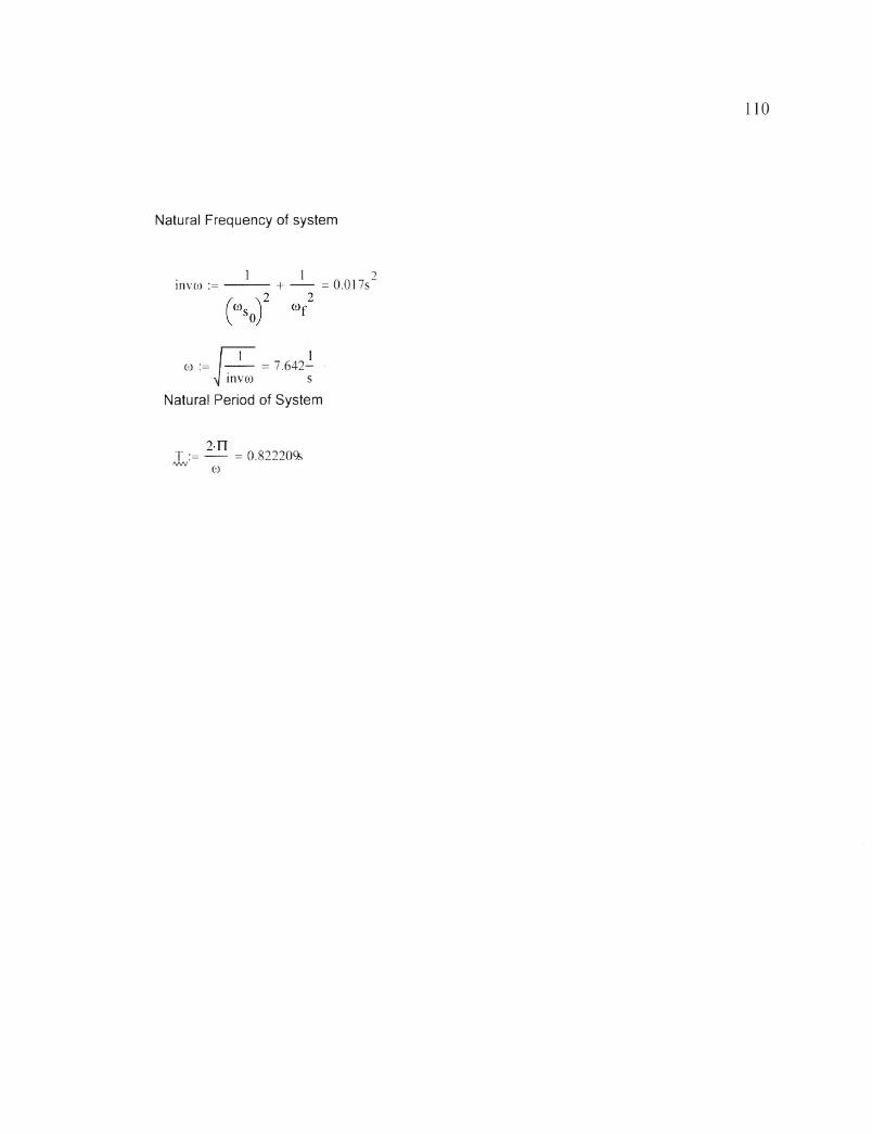
110
Natural Frequency of system
1 1 2 invco := ----------+ ------ = 0.017s
co := I—!— = 7.642- \j invco s
Natural Period of System
T := — = 0.82220%/wv co
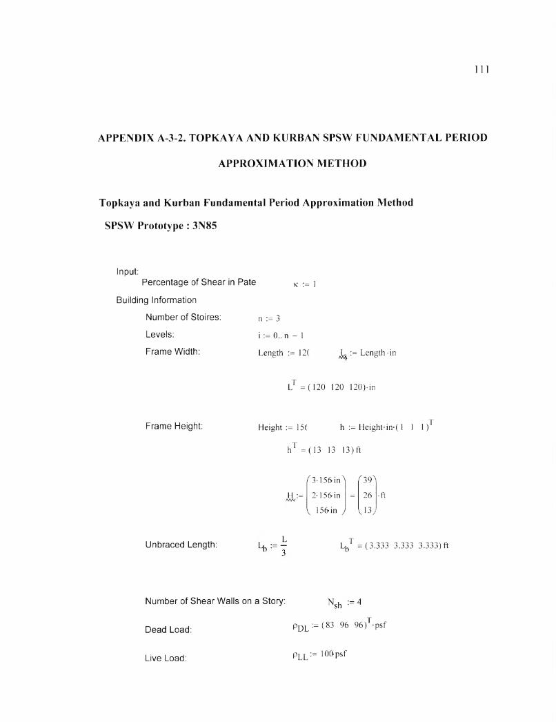
I l l
APPENDIX A-3-2. TOPKAYA AND KURBAN SPSW FUNDAMENTAL PERIOD
APPROXIMATION METHOD
Topkaya and Kurban Fundamental Period Approximation Method
SPSW Prototype: 3N85
Input:Percentage of Shear in Pate K := i
Building Information
Number of Stoires: n := 3
Levels: i : = 0 . . n - l
Frame Width: Length := 12C L. := Length-in
LT =(120 120 120)-in
Frame Height: Height := 15( h := Height in ( 1 1 1)
hT =(13 13 13) ft
,T
( 3-156-in^ ( 39 1
H := 2156in = 26 -ftWVv 156in J Vl3y
Unbraced Length: LbT =(3.333 3.333 3.333) ft
Number of Shear Walls on a Story:
Dead Load: pDL := (83 96 96)T psf
Live Load: PLl := lOOpsf

112
Seismic Design Acceleration:
SDS := 1.0 /
Sds := 1.0 /
Sdl := 0.7S
Material Properties
Web Plate
Steel Web Yield Strength:
Ratio of expected yield stress to the minimum yield stress:
Boundary ElementsSteel Yield Strength:
Ration of expected yield stress to the minimum yield stress:
Steel Modulus of Elasticity:
Steel Modulus of Rigidity:
Effective Length factor:
CodeBending phi factor
Tension phi factor
Shear phi factor
Compression phi factor
Fyweb := 36'ksi
^yw • 1.3
Fy := 50ksi
Ry := L]
E := 29000 ksi
G := 11.5106 psiAAA/ r
K := l.CAAAA
* b := 0.S
♦ t := 0.S
<t.v :=LC
♦ c : = 0 5
Braced member phi factor ^)br := 0.7f
ASTM A36
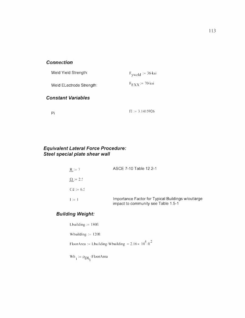
113
Connection
Weld Yield Strength: FyWeld := 36ksi
Weld ELectrode Strength: FEXX:= 7(>ksi
Constant Variables
pj n := 3.1415926
Equivalent Lateral Force Procedure: Steel special plate shear wall
R ;=7 ASCE 7-10 Table 12.2-1AAAt
Q := 2 .fAAAA
Cd := 6.f
I := i Importance Factor for Typical Buildings w/outlargeimpact to community see Table 1.5-1
Building Weight:
Lbuilding := 180ft
Wbuilding := 120ft
FloorArea := Lbuilding-Wbuilding = 2.16x 104-ft2
Wh. := Pql.- Floor Area

Wh =
1.793 x 10'
2.074 x 10'
2.074 x 10'
kip
FlrW := s tack |w hQ,Wh j , Wh 2j
FlrW
1.793x 10
2.074 x 10
V2.074x 10
kip
W - V FlrW. = 5.94 x 10 -kit/WW / J 1 r
WEB PLATE DESIGN PROPERTIES
Standard Steel Plate Thicknesses
t,wSTD •_ L 1 _ L J . _ L 2 J L J . J L 116 8 16 4 16 8 16 2 16 8

115
Gauge Steel Defined
Wg ■
\
V
0
0
0
0.2391
0.2242
0.2092
0.1943
0.1793
0.1644
0.1495
0.1345
0.1198
0.1046
0.0897
0.0747
0.0673
0.0598
0.0538
0.0478
0.0418
0.0359
0.0329
0.0299
0.0269
0.0239^
in
Steel Gauge begins at 3
Web Plate Thickness Per Story
wSTD0( 0.0625^
tw§ n = 0.1198 •in
twg9 ,
v0.1495y
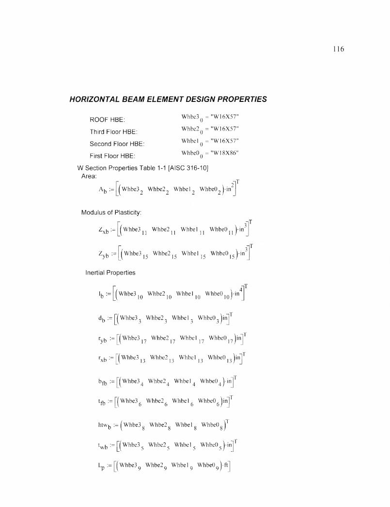
116
HORIZONTAL BEAM ELEMENT DESIGN PROPERTIES
ROOF HBE: Whbe30 = "W16X57"
Third Floor HBE: Whbe2() = "W16X57"
Second Floor HBE: Whbel Q = "W16X57"
First Floor HBE: Whbe0() = "W18X86"
W Section Properties Table 1-1 [AISC 316-10] Area:
. 2~|TAb := Whbe3„ Whbe2„ Whbel „ WhbeO„ -in'Y
Modulus of Plasticity:
,)z x b :" Whbe3 j j Whbe2 ] Whbel x ] WhbeO ] )in3
Zyb := [ Whbe3 j 5 Whbe2J5 Whbel |5 WhbeO ]5 )-in3
l bWhbe3 jQ Whbe2 ]Q Whbel 1() WhbeO ]Q |in 4
■ iT
• nT
Inertial Properties
.1db :=[7whbe33 Whbe23 Whbel 3 WhbeO3 jinjT
ryb := g w h b e3 17 Whbe2]? Whbel ]? WhbeO 1?)inj
rxb := [ (Whbe3 i3 w hb e2 13 Whbel ]3 WhbeO )3)inJ
bf b :=^W hbe34 Whbe24 Whbel 4 Whbe04 j-inj
tfb ;= [ ( whbe3 6 Whbe26 Whbel 6 WhbeO6jinJ
htwb := ^Whbe3g Whbe2g Whbel g WhbeO J
twb := r(w hbe35 Whbe2$ Whbel 5 WhbeO^-inj1
L p:= ^W hbe39 Whbe29 Whbel g Whbe09 )-ftj
• iT
iT
\T

Vertical Boundary Element Design Properties
Third Floor VBE: Wvbe3 Q =
Second Floor VBE: Wvbe2 Q =
First Floor VBE: Wvbel Q =
W Section Properties Table 1-1 [AISC 316-10]
Area:
Ac : [ Wvbe32 Wvbe22 Wvbel A in 2
Modulus of Plastcity:
3Z •= xc *
^yc
|W vbe311 Wvbe211 Wvbel ^ j i n
Wvbe3 Wvbe215 Wvbel 15
Inertial Properties:
Ic :=[(W vbe3 |0 Wvbe2|0 Wvbel ,„ )
dc := ^W vbe33 Wvbe23 Wvbel 3 jinj
ryC := [(W vbe317 Wvbe217 Wvbel jinj
rxe := [( Wvbe3 J3 Wvbe2 J3 Wvbel ]3 jinj
iT
m]
• 1T m]iTbfc :=[(W vbe34 Wvbe2^ Wvbel^j inj
tfc ^W vbe36 Wvbe2^ Wvbel 6 j-inJT
htwc := ( Wvbe3 g Wvbe2 g Wvbe 1 g jT
twc ^ Wvbe3 Wvbe2^ Wvbel 5 jinJT
Plastic Development Length:
LpC :=^W vbe39 Wvbe29 Wvbel
kdet := [(Wvbe322 Wvbe222 Wvbel 22 j-inj7
"W14X159
"W14X211
MW14X211

118
Angle of Inclination
a. := atan 1
1 +tw LWj l
2-A
1 + tw *h .■Wj iw3
360 L L. Al e. , b.
^0.707^180
a deg a ' n
( 40.496^
a = 0.674 38.646
v 0.66 y v37.807y
Length of beam from centerline: Lcf := L - dc
Application of Topkaya's Method: Upper Bound
Define Necessary Parameters
Thickness of Web-Plate: ptk„ := t,„ =0.063inu wo
Height of Web-Plate: piwu := h Q = 156in
Column Moment of Inertia: IyBEu:= = 19x lo3-ir|4
2Column Cross-Sectional Area: AVBEu: =Ac =46.7 in
Column Depth: dVBEu:= dc = 15-in

119
Cross-Sectional Area of Colunm Flange:
. 2Aflu := tfco bfcQ = 18-564in
Cross-Sectional Area of Column Flange:
Mass per story:
^webu * ( Cq ‘ detQjVcQ 7.45in. 2
^tory *W
32.2-g- 156-in3 lb
= 1.183 x 10 —in
Zalkas Factor: iv :=
r 0.493^
0.653
0.770
0.812
0.842
0.863
0.879
0.892
0.902
0.911)V
Calculate Necessary Q values
Q]upper := Aflu(°-5-Plwu + dVBEi) = L726x ^ ' i "3
S upper := Q]upper + Aw ebu°-5'(Plwu + dVBEi) = 2-363x 10'3 . 3 in
Supper A VBEu(p1wu + dVBEi) " 7‘986x 1()3' in3
(Plwu )2 3 3Q4upper := Q3upper + ---- Ptku = 8176x 10 in

120
Calculate P 1 and p 2
2 2 Ql upper + S upper , 8 . 6
Pj - dVBEu_ l 725x 10 inwc0
2 2:= ^ u p p e , + S upper _ |()n
2 lp tk u
Calculate Total p
p := pj + p2 = 1.632x 10U -in6
Determine Moment of Inertia for the Wall with respect to the Neutral Axis
Centroid of Web-VBE Interface:
0 '5' tfcj' twi-tfci + (°-5-h i)-(h i-tWj) + (°-5'tfcj + h ; -d. := ----------- 7— = ...-in
2-twi '( tfci) + *Wj
Averaged Centroid: dsys := mean(d) = 6.5ft
Moment of Inertia for 1 3 2 5 .4Web-VBE Interface: *w := ^ 'P tku 'P lwu + 2 AVBEiidsys + 2 I VBEu = 5-918x 10 in

121
Calculate Approximate Fundamental Period of SPSW
Application of Topkaya's Method: Lower Bound
Define Necessary Parameters
Thickness of Web-Plate: ptk, := t = 0.15-inn-1
Height of Web-Plate: piw, := h = 156in
Column Moment of Inertia: Iy B£i:= Ic = 2.66x l 03-in4n-1
2Column Cross-Sectional Area: A VBEj := A c = 62-in
Column Depth: d VBE1:= dc = 15.7-in
Cross-Sectional Areaof Colunm Flange: Af l l := tfcn_ , 'b fcn_ 1 = 24-648in
Fundamental Period: T,upper ' + ------- = 0.883s2 2 f fbu su
n-1
Cross-Sectional Area ,of Column Flange: A webl := e •twc'n-1

122
Calculate Necessary Q values
Qllower := Afir(0-5-plwj + dVBE|) = 2.31 x 10³-in3
.3 . 3S lo w er Qllower + Awebl'°-5'(Plwl + dVBEj) “ 3-147x 10 in
.4 . 3S lo w er AVBEl(Plwl + dVBEj) ~ 1 065x 10 -in
(Plwl)2 4 3Q41ower := Q31ower + ~ J -----Ptkl = 1-Hx 10 -in
Calculate p 1 and (3 2
2 2 ^1 lower + S low er 8 . 6
P |j VBE1- 2*441 x 10 -in
twCn -l
2 2^3 lower + S low er ll . 6
B91 := ----------------------------- plwi = 1.234x 10 -in21 2-ptk, 1
Calculate Total (3
^ : = P n + P 2I = 1.237x 10¹¹ -in6
Determine Moment of Inertia for the Wall with respect to the Neutral Axis
Centroid of Web-VBE Interface:
°-5' tfci' twi'tfci + (°-5'h i)'(^h i‘twij + + h i _ ‘fC j^ fC j 'Vd. := ----------- 7— = ...-in
1 2 ' S f tfci ) + h *’twi

123
Averaged Centroid: d mean(d) = 6 .5ft
Moment of Inertia for 1 3 2Web-VBE Interface: !w l := ~ Ptkl Plwl + 2 AVBEIdsys + 2 IVBE1:
Calculate Effective Shear Area
i 2'w 2" r>"2-inEffective Shear Area: KA . := — = 2.832-Wl p
Calculate Bending and Shearing Natural Frequencies
0 5595 I ^ ^wlBending Natural Fequency: f , . := rf •—1 I-----------= 5 .437-H2n~' |H Qj 2 J mstory
Shearing Natural Frequency: f , := rf ------------= 1.341-H2n -l 4-Hq J ^ to ry
Calculate Approximate Fundamental Period of SPSW
T *=Fundamental Period: lower • — + — = 0.768s 2 2
fbl fsl
8.07 x 10⁵-in4

124
APPENDIX A-4-1. lO-STORY SPSW PANEL ZONE OPENSEES CODE
# SPSW PROTOTYPE: 10W10 0# PANELZONE MODELING WITH MO DIF ICAT ION AT ROOF LEVEL# d e f i n e e l a s t i c p a n e l z o n e e l e m e n t s ( a s s u m e r i g i d )# e l e m P a n e l Z o n e 2 D c r e a t e s 8 e l a s t i c e l e m e n t s t h a t f o r m a r e c t a n g u l a r p a n e l z o n e# r e f e r e n c e s p r o v i d e d i n e l e m P a n e l Z o n e 2 D . t e l# n o t e : t h e n o d e l D a n d e l e l D o f t h e u p p e r l e f t c o r n e r o f t h e PZ m u s t b e i m p o r t e d# e l e l D c o n v e n t i o n : 5 0 0 x y a , 5 0 0 = p a n e l z o n e e l e m e n t , x = P i e r # , y = F l o o r ## " a " c o n v e n t i o n : d e f i n e d i n e l e m P a n e l Z o n e 2 D . t e l , b u t 1 = t o p l e f t e l e m e n tset Apz 1100.0; # a r e a o f p a n e l z o n e e l e m e n t ( m a k e m u c h l a r g e r t h a n A o f f r a m e e l e m e n t s )set E 29000 . 0;set Ipz 1 . 0 e 5 ; # m o m e n t o f i n t e r t i a o f p a n e l z o n e e l e m e n t ( m a k e m u c h l a r g e r t h a n I o f f r a m e e l e m e n t s )# e l e m P a n e l Z o n e 2 D e l e l D n o d e R E A_P Z I _ P Z t r a n s f T a ge 1 e m P a n e 1 Z o n e 2 D 500121 1201 $E $Apz $Ipz $PDeltaTransf; # P i e r 1 , F l o o rZe l e m P a n e l Z o n e 2 Do
500221 2201 $E $Apz $ Ipz $PDeltaTransf; # P i e r 2 , F l o o rze l e m P a n e l Z o n e 2 DQ
500131 1301 $E $Apz $Ipz $PDeltaTransf; # P i e r 1, F l o o rO
e l e m P a n e 1 Z o n e 2 D3e l e m P a n e l Z o n e 2 D
500231 2301 $E $Apz $ Ipz $PDeltaTransf; # P i e r 2 , F l o o r
500141 1401 $E $Apz $Ipz $PDeltaTransf ; # P i e r 1 , F l o o r*±
# [ J T 3 0 1 - 2 7 ] c h a n g e F l o o r 4 t o R o o f 2 / 2 5 / 2 0 1 5 R o o f C h a n g e d t o F l o o r 4e 1 e m P a n e l Z o n e 2 DA
500241 2401 $E $Apz $Ipz $PDeltaTransf ; # P i e r 2 , F l o o r
# [J T 3 0 1 - 2 8 ] c h a n g e F l o o r 4 F l o o r 4
t o R o o f CHANGE; 2 / 2 5 / 2 0 1 5 R o o f <C h a n g e d t o
e l e m P a n e l Z o n e 2 Dcr
500151 1501 $E $Apz $ Ipz $PDeltaTransf; # P i e r 1 , F l o o rbe l e m P a n e l Z o n e 2 Dc
500251 2501 $E $Apz $Ipz $PDeltaTransf; # P i e r 2 , F l o o rDe l e m P a n e l Z o n e 2 D 500161 1601 $E $Apz $Ipz $PDeltaTransf; # P i e r 1 , F l o o rbe l e m P a n e l Z o n e 2 D 500261 2601 $E $Apz $Ipz $PDeltaTransf; # P i e r 2 , F l o o rbe l e m P a n e l Z o n e 2 D7e l e m P a n e l Z o n e 2 D7e l e m P a n e l Z o n e 2 D8
500171 1701 $E $Apz $Ipz $PDeltaTransf; # P i e r 1 , F l o o r
500271 2701 $E $Apz $Ipz $PDeltaTransf; # P i e r 2 , F l o o r
500181 1801 $E $Apz $Ipz $PDeltaTransf; # P i e r 1 , F l o o r

125
elemPanelZone2D 500281 2801 $E $Apz $Ipz $PDeltaTransf; # P i e r 2 , F l o o r
elemPanelZone2D 500191 1901 $E $Apz $Ipz $PDeltaTransf; # P i e r 1 , F l o o r 9elemPanelZone2D 500291 2901 $E $Apz $Ipz $PDeltaTransf; # P i e r 2 , F l o o r 9# e l e I D { 5 0 0 1 1 0 1 5 0 0 2 1 0 1 5 0 0 1 1 1 1 5 0 0 2 1 1 1 } n o d e R { 1 1 0 0 0 1 2 1 0 0 0 1 1 1 1 0 0 1 2 1 1 0 0 1 } $E $ A p z $ I p z $ P D e l t a T r a n s f# p r o c e l e m P a n e l Z o n e 2 D { e l e l D n o d e R E A _P Z I__PZ t r a n s f T a g }foreach elelD {5001101 5002101 5001111 5002111} nodeR {llQOOl 210001 111001 211002} {set A_PZ 1100.0; # a r e a o f p a n e l z o n e e l e m e n t ( m a k e m u c h l a r g e r t h a n Ao f f r a m ee l e m e n t s )set E 29000 . 0;set I_PZ 1. 0 e 5 ;set transfTag 1;# d e f i n e p a n e l z o n e n o d e sset node_xy01 $nodeR; # t o p l e f t o f j o i n t
[expr $node__xy01 + 1][expr $node__xy01 + 2][expr $node_xy01 + ][expr $node_xy01 + 4]
set node_xy02 set node_xy03 set node_xy04 set node_xy05m i d d l e ,h o r i z o n t a l r i g h t ) set node_xy06 [expr $node_xy01
[expr $node__xy01 [expr $node_xy0i [expr $node_xy01 [expr ($node__xy01
# t o p l e f t o f j o i n t# t o p r i g h t o f j o i n t# t o p r i g h t o f j o i n t# m i d d l e r i g h t o f j o i n t ( v e r t i c a l
5] ;6] ;
] ;S] ; )/K
# b t m r i g h t o f j o i n t# b t m r i g h t o f j o i n t# b t m l e f t o f j o i n t# b t m l e f t o f j o i n t+ 10]; # m i d d l e l e f t o f j o i n t
set node_xy07 set node_xy08 set node_xy0 9 set node_xyl0( v e r t i c a l
m i d d l e , h o r i z o n t a l l e f t ) set node_xy6 [expr ( $ n o d e _ _ x y 0 1 - 1 ) / set node_xy7 [expr ($ n o d e _ _ x y 0 1 - 1 ) /# c r e a t e e l e m e n t I D s a s a f u n c t i o n o f f i r s t i n p u t e l e l D (8 p e r p a n e l z o n e )set xl $eleID; # l e f t e l e m e n t o n t o p o f p a n e l z o n e
+ 6 ] ; # b t m c e n t e r o f j o i n t + 3 ; # t o p c e n t e r o f j o i n t
1 ] ; # r i g h t e l e m e n t o n t o p o f p a n e l z o n e2 ] ; # t o p e l e m e n t o n r i g h t s i d e o f p a n e l z o n e3 ] ; # b t m e l e m e n t o n r i g h t s i d e o f p a n e l z o n e4 ] ; # r i g h t e l e m e n t o n b t m o f p a n e l z o n e
set x2 [expr $xl +set x3 [expr $xl +set x4 [expr $xl +set x5 [expr $xl +- 1-
C:\Users\Benjamin\Desktop\A-4-1.tcl Monday, March 21, 2016 7:56 PMset x6 [expr $xl + 5 ] ; # l e f t e l e m e n t o n b t m o f p a n e l z o n eset x7 [expr $xl + 6 ] ; # b t m e l e m e n t o n l e f t s i d e o f p a n e l z o n eset x8 [expr $xl + 7 ] ; # t o p e l e m e n t o n l e f t s i d e o f p a n e l z o n e# c r e a t e p a n e l z o n e e l e m e n t s# t a g n d l n d J A__PZ E I _ P Z t r a n s f T a gelement elasticBeamColumn $xl $node_xy02 $node_xy7 $A_PZ $E $1 PZ $transfTag;
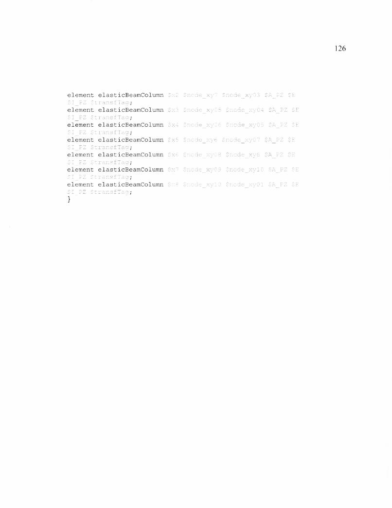
126
element elasticBeamColumn $x2 $node_xy7 $node_xy03 $A__PZ $E $I_PZ $transfTag;element elasticBeamColumn $x3 $node__xy05 $node_xy04 $A__PZ $E $I_PZ $transfTag;element elasticBeamColumn $x4 $node_xy0 6 $node_xy05 $A_PZ $E $I_PZ $transfTag;element elasticBeamColumn $x5 $node_xy6 $node_xy07 $A_PZ $E $I__PZ $transfTag;element elasticBeamColumn $x6 $node_xy08 $node_xy6 $A__PZ $E $I__PZ $transfTag;element elasticBeamColumn $x7 $node_xy0 9 $node__xylO $A_PZ $E $I_PZ $transfTag;element elasticBeamColumn $x8 $node_xylO $node_xy01 $A_PZ $E $I_PZ $transfTag;}

127
APPENDIX A-6-1. VERIFICATION OF PROPOSED METHOD WITH
VALIDATION PROTOTYPE
Validation of Kean's Fundamental Period Approxiamtion Method
SPSW PROTOTYPE: 3K100
Building Parameters
Building Height (feet)
H := 3SAAA/
Base-Shear Participation Level
V := 1AA A /
Bay-Width (feet)
ASCE 7-10 Equation 12-8-2 Parameters
c t := 0.02
x := 0.75

128
Proposed Method Coefficients
a c := 0.189'
Pc := 0.523‘
Px := - 0.209‘
epc
?pc
a x := 2 -136f e a x :
ax *
0a C := -l.B 46( 0p x :
Y a C := 3.187C Ypx
Proposed Method
faC := 0a C V+ YaC = L341
fpc := 0pc v + y p c = 0 861
W -= ®ax ^ + Y ax = 0-967
fp x := 0p xV+ Ypx = 0-943
P c fpcfC := a C fa C L = 0.78
f, := CL,-f„v-L^X = 1.264x ax
xf
T = 0.503 seconds
TpE *— 0.48(
Errortf e - t
lFE3.466%
= 0.767
= 0.093'
- 0.289^
= 0.677'
= 0.633:
= 0.3095