Functions of Matrices

Higham, Nicholas J.

2005

MIMS EPrint: 2005.21

Manchester Institute for Mathematical SciencesSchool of Mathematics

The University of Manchester

Reports available from: http://eprints.maths.manchester.ac.uk/And by contacting: The MIMS Secretary

School of Mathematics

The University of Manchester

Manchester, M13 9PL, UK

ISSN 1749-9097

F.13 Functions of Matrices1

Matrix functions are used in many areas of linear algebra and arise in numerous applica-

tions in science and engineering. The most common matrix function is the matrix inverse;

it is not treated specifically in this article, but is covered in Chapter B. This article is

concerned with general matrix functions as well as the specific cases of matrix square

roots, trigonometric functions, and the exponential and logarithmic functions.

The specific functions just mentioned can all be defined via power series or as the

solution of nonlinear systems. For example, cos(A) = I −A2/2!+A4/4!−· · ·. However, a

general theory exists from which a number of properties possessed by all matrix functions

can be deduced and which suggest computational methods. This article treats general

theory, then specific functions, and finally outlines computational methods.

Proofs of the facts in this article can be found in one or more of [Hig], [HJ91] or [LT85],

unless otherwise stated.

1 General Theory

Definitions:

A function of a matrix can be defined in several ways, of which the following three are

the most generally useful.

• Jordan canonical form definition. Let A ∈ Cn×n have the Jordan canonical form

1Nicholas J. Higham, School of Mathematics, The University of Manchester, Sackville Street, Manch-

ester, M60 1QD, UK (higham@ma.man.ac.uk, http://www.ma.man.ac.uk/~higham/). For Handbook

of Linear Algebra, edited by Hogben, Brualdi, Greenbaum, and Mathias, CRC Press. Version dated

November 7, 2005.

1

Z−1AZ = JA = diag(J1(λ1), J2(λ2), . . . , Jp(λp)), where Z is nonsingular,

Jk(λk) =

λk 1

λk. . .

. . . 1

λk

∈ Cmk×mk , (1)

and m1 + m2 + · · · + mp = n. Then

f(A) := Zf(JA)Z−1 = Z diag(f(Jk(λk)))Z−1, (2)

where

f(Jk(λk)) :=

f(λk) f ′(λk) . . .f (mk−1))(λk)

(mk − 1)!

f(λk). . .

...

. . . f ′(λk)

f(λk)

. (3)

• Polynomial interpolation definition. Denote by λ1, . . . , λs the distinct eigenvalues of

A and let ni be the index of λi, that is, the order of the largest Jordan block in

which λi appears. Then f(A) := r(A), where r is the unique Hermite interpolating

polynomial of degree less than∑s

i=1 ni that satisfies the interpolation conditions

r(j)(λi) = f (j)(λi), j = 0: ni − 1, i = 1: s. (4)

Note that in both these definitions the derivatives in (4) must exist in order for f(A)

to be defined. The function f is said to be defined on the spectrum of A if all the

derivatives in (4) exist.

• Cauchy integral definition.

f(A) :=1

2πi

∫

Γ

f(z)(zI − A)−1 dz, (5)

where f is analytic inside a closed contour Γ that encloses σ(A).

2

When the function f is multivalued and A has a repeated eigenvalue occurring in more

than one Jordan block (i.e., A is derogatory), the Jordan canonical form definition has

more than one interpretation. Usually, for each occurrence of an eigenvalue in different

Jordan blocks the same branch is taken for f and its derivatives. This gives a primary

matrix function. If different branches are taken for the same eigenvalue in two different

Jordan blocks then a nonprimary matrix function is obtained. A nonprimary matrix

function is not expressible as a polynomial in the matrix, and if such a function is obtained

from the Jordan canonical form definition (2) then it depends on the matrix Z. In most

applications it is primary matrix functions that are of interest. For the rest of this article

f(A) is assumed to be a primary matrix function, unless otherwise stated.

Facts:

1. The Jordan canonical form and polynomial interpolation definitions are equivalent.

Both definitions are equivalent to the Cauchy integral definition when f is analytic.

2. f(A) is a polynomial in A and the coefficients of the polynomial depend on A.

3. f(A) commutes with A.

4. f(AT ) = f(A)T .

5. For any nonsingular X, f(XAX−1) = Xf(A)X−1.

6. If A is diagonalizable, with Z−1AZ = D = diag(d1, d2, . . . , dn), then f(A) =

Zf(D)Z−1 = Z diag(f(d1), f(d2), . . . , f(dn))Z−1.

7. f(diag(A1, A2, . . . , Am)) = diag(f(A1), f(A2), . . . , f(Am)).

8. Let f and g be functions defined on the spectrum of A. (a) If h(t) = f(t) + g(t)

then h(A) = f(A) + g(A). (b) If h(t) = f(t)g(t) then h(A) = f(A)g(A).

3

9. Let G(u1, . . . , ut) be a polynomial in u1, . . . , ut and let f1, . . . , ft be functions defined

on the spectrum of A. If g(λ) = G(f1(λ), . . . , ft(λ)) takes zero values on the spec-

trum of A then g(A) = G(f1(A), . . . , ft(A)) = 0. For example, sin2(A)+cos2(A) = I,

(A1/p)p = A, and eiA = cos A + i sin A.

10. Suppose f has a Taylor series expansion

f(z) =∞∑

k=0

ak(z − α)k

(

ak =f (k)(α)

k!

)

with radius of convergence r. If A ∈ Cn×n then f(A) is defined and is given by

f(A) =∞∑

k=0

ak(A − αI)k

if and only if each of the distinct eigenvalues λ1, . . . , λs of A satisfies one of the

conditions

(a) |λi − α| < r,

(b) |λi−α| = r and the series for fni−1(λ), where ni is the index of λi, is convergent

at the point λ = λi, i = 1: s.

11. [Dav73], [Des63], [GVL96, 1996, Thm. 11.1.3]. Let T ∈ Cn×n be upper triangular

and suppose that f is defined on the spectrum of T . Then F = f(T ) is upper

triangular with fii = f(tii) and

fij =∑

(s0,...,sk)∈Sij

ts0,s1ts1,s2

. . . tsk−1,skf [λs0

, . . . , λsk],

where λi = tii, Sij is the set of all strictly increasing sequences of integers that start

at i and end at j, and f [λs0, . . . , λsk

] is the kth order divided difference of f at

λs0, . . . , λsk

.

4

Examples:

1. For λ1 6= λ2,

f

([

λ1 α

0 λ2

])

=

[

f(λ1) αf(λ2) − f(λ1)

λ2 − λ1

0 f(λ2)

]

.

For λ1 = λ2 = λ,

f

([

λ α

0 λ

])

=

[

f(λ) αf ′(λ)

0 f(λ)

]

.

2. Compute eA for the matrix

A =

−7 −4 −3

10 6 4

6 3 3

.

We have A = XJAX−1, where JA = [0] ⊕ [10

11] and

X =

1 −1 −1

−1 2 0

−1 0 3

.

Hence, using the Jordan canonical form definition, we have

eA = XeJAX−1 = X([1] ⊕ [ e

0ee])X−1

=

1 −1 −1

−1 2 0

−1 0 3

1 0 0

0 e e

0 0 e

6 3 2

2 2 1

2 1 1

=

6 − 7e 3 − 4e 2 − 3e

−6 + 10e −3 + 6e −2 + 4e

−6 + 6e −3 + 3e −2 + 3e

.

3. Compute√

A for the matrix in Example 1. To obtain the square root, we use the

polynomial interpolation definition. The eigenvalues of A are 0 and 1, with indices

5

1 and 2, respectively. The unique polynomial r of degree at most 2 satisfying the

interpolation conditions r(0) = f(0), r(1) = f(1), r′(1) = f ′(1) is

r(t) = f(0)(t − 1)2 + t(2 − t)f(1) + t(t − 1)f ′(1).

With f(t) = t1/2, taking the positive square root, we have r(t) = t(2−t)+t(t−1)/2,

and therefore

A1/2 = A(2I − A) + A(A − I)/2 =

−6 −3.5 −2.5

8 5 3

6 3 3

.

4. Consider the mk × mk Jordan block Jk(λk) in (1). The polynomial satisfying the

interpolation conditions (4) is

r(t) = f(λk) + (t − λk)f′(λk) +

(t − λk)2

2!f ′′(λk) + · · · + (t − λk)

mk−1

(mk − 1)!f (mk−1)(λk),

which of course is the first mk terms of the Taylor series of f about λk. Hence, from

the polynomial interpolation definition,

f(Jk(λk)) = r(Jk(λk))

= f(λk)I + (Jk(λk) − λkI)f ′(λk) +(Jk(λk) − λkI)2

2!f ′′(λk) + · · ·

+(Jk(λk) − λkI)mk−1

(mk − 1)!f (mk−1)(λk).

The matrix (Jk(λk) − λkI)j is zero except for 1s on the jth superdiagonal. This

expression for f(Jk(λk)) is therefore equal to that in (3), confirming the consistency

of the first two definitions of f(A).

2 Matrix Square Root

Definitions:

6

Let A ∈ Cn×n. Any X such that X2 = A is a square root of A.

Facts:

1. If A ∈ Cn×n has no eigenvalues on R

− (the closed negative real axis) then there is a

unique square root X of A all of whose eigenvalues lie in the open right half-plane,

and it is a primary matrix function of A. This is the principal square root of A

and is written X = A1/2. If A is real then A1/2 is real. An integral representation is

A1/2 =2

πA

∫

∞

0

(t2I + A)−1 dt.

2. A Hermitian positive definite matrix A ∈ Cn×n has a unique Hermitian positive

definite square root.

3. [CL74] A singular matrix A ∈ Cn×n may or may not have a square root. A necessary

and sufficient condition for A to have a square root is that in the “ascent sequence”

of integers d1, d2, . . . defined by

di = dim(ker(Ai)) − dim(ker(Ai−1))

no two terms are the same odd integer.

4. A ∈ Rn×n has a real square root if and only if A satisfies the condition in the

previous fact and A has an even number of Jordan blocks of each size for every

negative eigenvalue.

5. The n × n identity matrix In has 2n diagonal square roots diag(±1). Only two of

these are primary matrix functions, namely I and −I. Nondiagonal but symmetric

nonprimary square roots of In include any Householder matrix I − 2vvT /(vTv)

(v 6= 0) and the identity matrix with its columns in reverse order. Nonsymmetric

7

square roots of In are easily constructed in the form XDX−1, where X is nonsingular

but nonorthogonal and D = diag(±1) 6= ±I.

Examples:

1. The Jordan block [00

10] has no square root. The matrix

0 1 0

0 0 0

0 0 0

has ascent sequence 2, 1, 0, . . . and so does have a square root—for example, the

matrix

0 0 1

0 0 0

0 1 0

.

3 Matrix Exponential

Definitions:

The exponential of A ∈ Cn×n, written eA or exp(A), is defined by

eA = I + A +A2

2!+ · · · + Ak

k!+ · · · .

Facts:

1. e(A+B)t = eAteBt holds for all t if and only if AB = BA.

2. The differential equation in n × n matrices

dY

dt= AY, Y (0) = C, A, Y ∈ C

n×n,

has solution Y (t) = eAtC.

8

3. The differential equation in n × n matrices

dY

dt= AY + Y B, Y (0) = C, A,B, Y ∈ C

n×n,

has solution Y (t) = eAtCeBt.

4. A ∈ Cn×n is unitary if and only if it can be written A = eiH , where H is Hermitian.

In this representation H can be taken to be Hermitian positive definite.

5. A ∈ Rn×n is orthogonal with det(A) = 1 if and only if A = eS with S ∈ R

n×n

skew-symmetric.

Examples:

1. Fact 5 is illustrated by the matrix

A =

[

0 α

−α 0

]

,

for which

eA =

[

cos α sin α

− sin α cos α

]

.

4 Matrix Logarithm

Definitions:

Let A ∈ Cn×n. Any X such that eX = A is a logarithm of A.

Facts:

1. If A has no eigenvalues on R− then there is a unique logarithm X of A all of

whose eigenvalues lie in the strip { z : −π < Im(z) < π }. This is the principal

logarithm of A, and is written X = log A. If A is real then log A is real.

9

2. If ρ(A) < 1,

log(I + A) = A − A2

2+

A3

3− A4

4+ · · · .

3. A ∈ Rn×n has a real logarithm if and only if A is nonsingular and A has an even

number of Jordan blocks of each size for every negative eigenvalue.

4. exp(log A) = A holds when log is defined on the spectrum of A ∈ Cn×n. But

log(exp(A)) = A does not generally hold unless the spectrum of A is restricted.

5. If A ∈ Cn×n is nonsingular then det(A) = exp(tr(log A)), where log A is any loga-

rithm of A.

Examples:

For the matrix

A =

1 1 1 1

0 1 2 3

0 0 1 3

0 0 0 1

we have

log(A) =

0 1 0 0

0 0 2 0

0 0 0 3

0 0 0 0

.

5 Matrix Sine and Cosine

Definitions:

The sine and cosine of A ∈ Cn×n are defined by

cos(A) = I − A2

2!+ · · · + (−1)k

(2k)!A2k + · · · ,

10

sin(A) = A − A3

3!+ · · · + (−1)k

(2k + 1)!A2k+1 + · · · .

Facts:

1. cos(2A) = 2 cos2(A) − I.

2. sin(2A) = 2 sin(A) cos(A).

3. cos2(A) + sin2(A) = I.

4. The differential equation

d2y

dt2+ Ay = 0, y(0) = y0, y′(0) = y′

0

has solution

y(t) = cos(√

At)y0 + (√

A)−1 sin(√

At)y′

0,

where√

A denotes any square root of A.

Examples:

1. For

A =

[

0 i α

i α 0

]

,

we have

eA =

[

cos α i sin α

i sin α cos α

]

.

2. For

A =

1 1 1 1

0 −1 −2 −3

0 0 1 3

0 0 0 −1

11

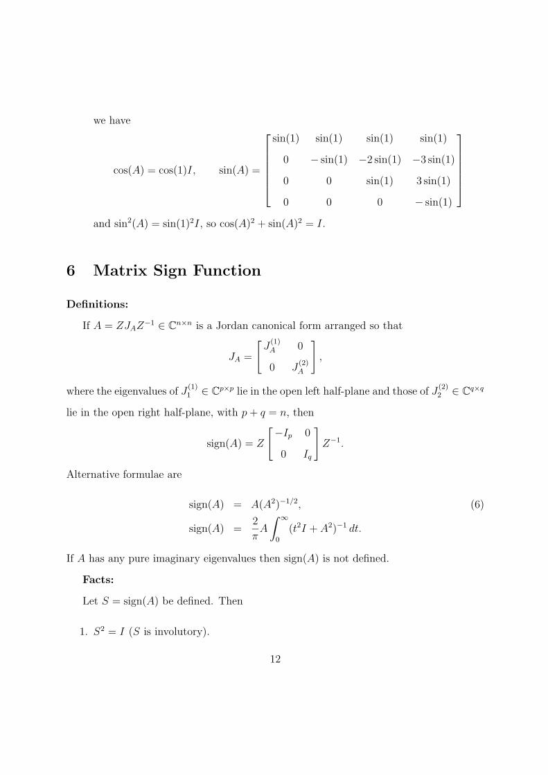
we have

cos(A) = cos(1)I, sin(A) =

sin(1) sin(1) sin(1) sin(1)

0 − sin(1) −2 sin(1) −3 sin(1)

0 0 sin(1) 3 sin(1)

0 0 0 − sin(1)

and sin2(A) = sin(1)2I, so cos(A)2 + sin(A)2 = I.

6 Matrix Sign Function

Definitions:

If A = ZJAZ−1 ∈ Cn×n is a Jordan canonical form arranged so that

JA =

[

J(1)A 0

0 J(2)A

]

,

where the eigenvalues of J(1)1 ∈ C

p×p lie in the open left half-plane and those of J(2)2 ∈ C

q×q

lie in the open right half-plane, with p + q = n, then

sign(A) = Z

[−Ip 0

0 Iq

]

Z−1.

Alternative formulae are

sign(A) = A(A2)−1/2, (6)

sign(A) =2

πA

∫

∞

0

(t2I + A2)−1 dt.

If A has any pure imaginary eigenvalues then sign(A) is not defined.

Facts:

Let S = sign(A) be defined. Then

1. S2 = I (S is involutory).

12

2. S is diagonalizable with eigenvalues ±1.

3. SA = AS.

4. If A is real then S is real.

5. If A is symmetric positive definite then sign(A) = I.

Examples:

1. For the matrix A in Example 2 of the previous subsection we have sign(A) = A,

which follows from (6) and the fact that A is involutory.

7 Computational Methods for General Functions

Many methods have been proposed for evaluating matrix functions. Three general ap-

proaches of wide applicability are outlined here. They have in common that they do not

require knowledge of Jordan structure and are suitable for computer implementation.

1. Polynomial and Rational Approximations

Polynomial approximations

pm(X) =m∑

k=0

bkXk, bk ∈ C, X ∈ C

n×n,

to matrix functions can be obtained by truncating or economizing a power series represen-

tation, or by constructing a best approximation (in some norm) of a given degree. How to

most efficiently evaluate a polynomial at a matrix argument is a nontrivial question. Pos-

sibilities include Horner’s method, explicit computation of the powers of the matrix, and

a method of Paterson and Stockmeyer [GVL96, Sec. 11.2.4], [PS73] that is a combination

of these two methods that requires fewer matrix multiplications.

13

Rational approximations rmk(X) = pm(X)qk(X)−1 are also widely used, particularly

those arising from Pade approximation, which produces rationals matching as many terms

of the Taylor series of the function at the origin as possible. The evaluation of rationals

at matrix arguments needs careful consideration in order to find the best compromise

between speed and accuracy. The main possibilities are

• Evaluating the numerator and denominator polynomials and then solving a multiple

right-hand side linear system.

• Evaluating a continued fraction representation (in either top-down or bottom-up

order).

• Evaluating a partial fraction representation.

Since polynomials and rationals are typically accurate over a limited range of matrices,

practical methods involve a reduction stage prior to evaluating the polynomial or rational.

2. Factorization Methods

Many methods are based on the property f(XAX−1) = Xf(A)X−1. If X can be found

such that B = XAX−1 has the property that f(B) is easily evaluated, then an obvious

method results. When A is diagonalizable, B can be taken to be diagonal, and evaluation

of f(B) is trivial. In finite precision arithmetic, though, this approach is reliable only

if X is well conditioned, that is, if the condition number κ(X) = ‖X‖‖X−1‖ is not too

large. Ideally, X will be unitary, so that in the 2-norm κ2(X) = 1. For Hermitian A, or

more generally normal A, the spectral decomposition A = QDQ∗ with Q unitary and D

diagonal is always possible, and if this decomposition can be computed then the formula

f(A) = Qf(D)Q∗ provides an excellent way of computing f(A).

For general A, if X is restricted to be unitary then the furthest that A can be reduced

14

is to Schur form: A = QTQ∗, where Q is unitary and T upper triangular. This decom-

position is computed by the QR algorithm. Computing a function of a triangular matrix

is an interesting problem. While Fact 11 of Subsection 1 gives an explicit formula for

F = f(T ), the formula is not practically viable due to its exponential cost in n. Much

more efficient is a recurrence of Parlett [Par76]. This is derived by starting with the

observation that since F is representable as a polynomial in T , F is upper triangular,

with diagonal elements f(tii). The elements in the strict upper triangle are determined

by solving the equation FT = TF . Parlett’s recurrence is:

Algorithm 1. Parlett’s recurrence.

fii = f(tii), i = 1: n

for j = 2: n

for i = j − 1:−1: 1

fij = tijfii − fjj

tii − tjj+(

j−1∑

k=i+1

fiktkj − tikfkj

)

/ (tii − tjj)

end

end

This recurrence can be evaluated in 2n3/3 operations. The recurrence breaks down

when tii = tjj for some i 6= j. In this case, T can be regarded as a block matrix T = (Tij),

with square diagonal blocks, possibly of different sizes. T can be reordered so that no

two diagonal blocks have an eigenvalue in common; reordering means applying a unitary

similarity transformation to permute the diagonal elements whilst preserving triangularity.

Then a block form of the recurrence can be employed. This requires the evaluation of the

diagonal blocks Fii = f(Tii), where Tii will typically be of small dimension. A general way

to obtain Fii is via a Taylor series. The use of the block Parlett recurrence in combination

15

with a Schur decomposition represents the state of the art in evaluation of f(A) for general

functions [DH03].

3. Iteration Methods

Several matrix functions f can be computed by iteration:

Xk+1 = g(Xk), X0 = A, (7)

where, for reasons of computational cost, g is usually a polynomial or a rational function.

Such an iteration might converge for all A for which f is defined, or just for a subset of

such A. A standard means of deriving matrix iterations is to apply Newton’s method

to an algebraic equation satisfied by f(A). The iterations most used in practice are

quadratically convergent, but iterations with higher orders of convergence are known.

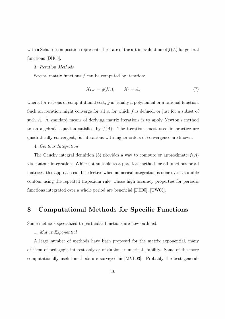
4. Contour Integration

The Cauchy integral definition (5) provides a way to compute or approximate f(A)

via contour integration. While not suitable as a practical method for all functions or all

matrices, this approach can be effective when numerical integration is done over a suitable

contour using the repeated trapezium rule, whose high accuracy properties for periodic

functions integrated over a whole period are beneficial [DH05], [TW05].

8 Computational Methods for Specific Functions

Some methods specialized to particular functions are now outlined.

1. Matrix Exponential

A large number of methods have been proposed for the matrix exponential, many

of them of pedagogic interest only or of dubious numerical stability. Some of the more

computationally useful methods are surveyed in [MVL03]. Probably the best general-

16

purpose method is the scaling and squaring method. In this method an integral power of

2, σ = 2s say, is chosen so that A/σ has norm not too far from 1. The exponential of the

scaled matrix is approximated by an [m/m] Pade approximant, eA/2s ≈ rmm(A/2s), and

then s repeated squarings recover an approximation to eA: eA ≈ rmm(A/2s)2s

. Symmetries

in the Pade approximant permit an efficient evaluation of rmm(A). The scaling and

squaring method was originally developed in [MVL78] and [War77], and it is the method

employed by MATLAB’s expm function. How best to choose σ and m is described in

[Hig05].

2. Matrix Logarithm

The (principal) matrix logarithm can be computed using an inverse scaling and squar-

ing method based on the identity log A = 2k log A1/2k

, where A is assumed to have no

eigenvalues on R−. Square roots are taken to make ‖A1/2k − I‖ small enough that an

[m/m] Pade approximant approximates log A1/2k

sufficiently accurately, for some suit-

able m. Then log A is recovered by multiplying by 2k. To reduce the cost of computing

the square roots and evaluating the Pade approximant, a Schur decomposition can be

computed initially so that the method works with a triangular matrix. For details, see

[CHKL01], [Hig01], [KL89, App. A].

3. Matrix Cosine and Sine

A method analogous to the scaling and squaring method for the exponential is the

standard method for computing the matrix cosine. The idea is again to scale A to have

norm not too far from 1 and then compute a Pade approximant. The difference is that

the scaling is undone by repeated use of the double-angle formula cos(2A) = 2 cos2 A− I,

rather than by repeated squaring. The sine function can be obtained as sin(A) = cos(A−π2I). See [SB80], [HS03], [HH05].

4. Matrix Square Root

17

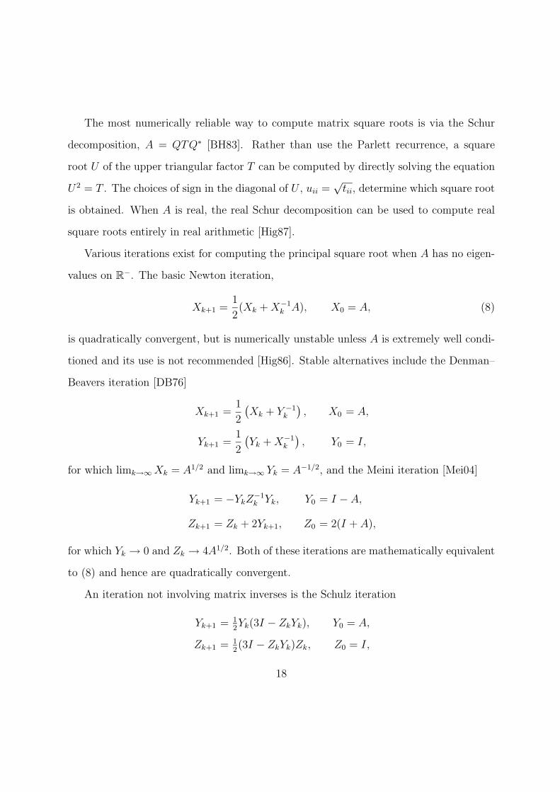
The most numerically reliable way to compute matrix square roots is via the Schur

decomposition, A = QTQ∗ [BH83]. Rather than use the Parlett recurrence, a square

root U of the upper triangular factor T can be computed by directly solving the equation

U2 = T . The choices of sign in the diagonal of U , uii =√

tii, determine which square root

is obtained. When A is real, the real Schur decomposition can be used to compute real

square roots entirely in real arithmetic [Hig87].

Various iterations exist for computing the principal square root when A has no eigen-

values on R−. The basic Newton iteration,

Xk+1 =1

2(Xk + X−1

k A), X0 = A, (8)

is quadratically convergent, but is numerically unstable unless A is extremely well condi-

tioned and its use is not recommended [Hig86]. Stable alternatives include the Denman–

Beavers iteration [DB76]

Xk+1 =1

2

(

Xk + Y −1k

)

, X0 = A,

Yk+1 =1

2

(

Yk + X−1k

)

, Y0 = I,

for which limk→∞ Xk = A1/2 and limk→∞ Yk = A−1/2, and the Meini iteration [Mei04]

Yk+1 = −YkZ−1k Yk, Y0 = I − A,

Zk+1 = Zk + 2Yk+1, Z0 = 2(I + A),

for which Yk → 0 and Zk → 4A1/2. Both of these iterations are mathematically equivalent

to (8) and hence are quadratically convergent.

An iteration not involving matrix inverses is the Schulz iteration

Yk+1 = 12Yk(3I − ZkYk), Y0 = A,

Zk+1 = 12(3I − ZkYk)Zk, Z0 = I,

18

for which Yk → A1/2 and Zk → A−1/2 quadratically provided that ‖ diag(A−I, A−I)‖ < 1,

where the norm is any consistent matrix norm [Hig97].

5. Matrix sign function

The standard method for computing the matrix sign function is the Newton iteration

Xk+1 =1

2(Xk + X−1

k ), X0 = A,

which converges quadratically to sign(A), provided A has no pure imaginary eigenvalues.

In practice, a scaled iteration

Xk+1 =1

2(µkXk + µ−1

k X−1k ), X0 = A.

is used, where the scale parameters µk are chosen to reduce the number of iterations

needed to enter the regime where asymptotic quadratic convergence sets in. See [Bye87],

[KL92].

The Newton–Schulz iteration

Xk+1 =1

2Xk(3I − X2

k), X0 = A,

involves no matrix inverses but convergence is guaranteed only for ‖I − A2‖ < 1.

A Pade family of iterations

Xk+1 = Xkpℓm(1 − X2k)qℓm(1 − X2

k)−1, X0 = A,

is obtained in [KL91], where pℓm(ξ)/qℓm(ξ) is the [ℓ/m] Pade approximant to (1− ξ)−1/2.

The iteration is globally convergent to sign(A) for ℓ = m−1 and ℓ = m, and for ℓ ≥ m−1

is convergent when ‖I − A2‖ < 1, with order of convergence ℓ + m + 1 in all cases.

19

References

[BH83] Ake Bjorck and Sven Hammarling. A Schur method for the square root of a

matrix. Linear Algebra Appl., 52/53:127–140, 1983.

[Bye87] Ralph Byers. Solving the algebraic Riccati equation with the matrix sign

function. Linear Algebra Appl., 85:267–279, 1987.

[CHKL01] Sheung Hun Cheng, Nicholas J. Higham, Charles S. Kenney, and Alan J.

Laub. Approximating the logarithm of a matrix to specified accuracy. SIAM

J. Matrix Anal. Appl., 22(4):1112–1125, 2001.

[CL74] G. W. Cross and P. Lancaster. Square roots of complex matrices. Linear and

Multilinear Algebra, 1:289–293, 1974.

[Dav73] Chandler Davis. Explicit functional calculus. Linear Algebra Appl., 6:193–199,

1973.

[DB76] Eugene D. Denman and Alex N. Beavers, Jr. The matrix sign function and

computations in systems. Appl. Math. Comput., 2:63–94, 1976.

[Des63] Jean Descloux. Bounds for the spectral norm of functions of matrices. Numer.

Math., 15:185–190, 1963.

[DH03] Philip I. Davies and Nicholas J. Higham. A Schur–Parlett algorithm for com-

puting matrix functions. SIAM J. Matrix Anal. Appl., 25(2):464–485, 2003.

[DH05] Philip I. Davies and Nicholas J. Higham. Computing f(A)b for matrix func-

tions f . In Artan Borici, Andreas Frommer, Baalint Joo, Anthony Kennedy,

and Brian Pendleton, editors, QCD and Numerical Analysis III, volume 47 of

20

Lecture Notes in Computational Science and Engineering, pages 15–24. Spring-

er-Verlag, Berlin, 2005.

[GVL96] Gene H. Golub and Charles F. Van Loan. Matrix Computations. Johns Hop-

kins University Press, Baltimore, MD, USA, third edition, 1996.

[HH05] Gareth I. Hargreaves and Nicholas J. Higham. Efficient algorithms for the

matrix cosine and sine. Numerical Analysis Report 461, Manchester Centre

for Computational Mathematics, Manchester, England, February 2005. To

appear in Numerical Algorithms.

[Hig] Nicholas J. Higham. Functions of a Matrix: Theory and Computation. Book

in preparation.

[Hig86] Nicholas J. Higham. Newton’s method for the matrix square root. Math.

Comp., 46(174):537–549, April 1986.

[Hig87] Nicholas J. Higham. Computing real square roots of a real matrix. Linear

Algebra Appl., 88/89:405–430, 1987.

[Hig97] Nicholas J. Higham. Stable iterations for the matrix square root. Numerical

Algorithms, 15(2):227–242, 1997.

[Hig01] Nicholas J. Higham. Evaluating Pade approximants of the matrix logarithm.

SIAM J. Matrix Anal. Appl., 22(4):1126–1135, 2001.

[Hig05] Nicholas J. Higham. The scaling and squaring method for the matrix expo-

nential revisited. SIAM J. Matrix Anal. Appl., 26(4):1179–1193, 2005.

21

[HJ91] Roger A. Horn and Charles R. Johnson. Topics in Matrix Analysis. Cambridge

University Press, 1991.

[HS03] Nicholas J. Higham and Matthew I. Smith. Computing the matrix cosine.

Numerical Algorithms, 34:13–26, 2003.

[KL89] Charles S. Kenney and Alan J. Laub. Condition estimates for matrix functions.

SIAM J. Matrix Anal. Appl., 10(2):191–209, 1989.

[KL91] Charles S. Kenney and Alan J. Laub. Rational iterative methods for the matrix

sign function. SIAM J. Matrix Anal. Appl., 12(2):273–291, 1991.

[KL92] Charles S. Kenney and Alan J. Laub. On scaling Newton’s method for polar

decomposition and the matrix sign function. SIAM J. Matrix Anal. Appl.,

13(3):688–706, 1992.

[LT85] Peter Lancaster and Miron Tismenetsky. The Theory of Matrices. Academic

Press, London, second edition, 1985.

[Mei04] Beatrice Meini. The matrix square root from a new functional perspective:

Theoretical results and computational issues. SIAM J. Matrix Anal. Appl.,

26(2):362–376, 2004.

[MVL78] Cleve B. Moler and Charles F. Van Loan. Nineteen dubious ways to compute

the exponential of a matrix. SIAM Rev., 20(4):801–836, 1978.

[MVL03] Cleve B. Moler and Charles F. Van Loan. Nineteen dubious ways to compute

the exponential of a matrix, twenty-five years later. SIAM Rev., 45(1):3–49,

2003.

22

[Par76] B. N. Parlett. A recurrence among the elements of functions of triangular

matrices. Linear Algebra Appl., 14:117–121, 1976.

[PS73] Michael S. Paterson and Larry J. Stockmeyer. On the number of nonscalar

multiplications necessary to evaluate polynomials. SIAM J. Comput., 2(1):60–

66, 1973.

[SB80] Steven M. Serbin and Sybil A. Blalock. An algorithm for computing the matrix

cosine. SIAM J. Sci. Statist. Comput., 1(2):198–204, 1980.

[TW05] L. N. Trefethen and J. A. C. Weideman. The fast trapezoid rule in scientific

computing. Paper in preparation, 2005.

[War77] Robert C. Ward. Numerical computation of the matrix exponential with ac-

curacy estimate. SIAM J. Numer. Anal., 14(4):600–610, 1977.

23