Functional-coefficient cointegrating regression with endogeneity

Han-Ying Liang, Yu Shen and Qiying Wang

Tongji University, Tongji University and The University of Sydney

May 12, 2017

Abstract

This paper explores nonparametric estimation of functional-coefficient cointegrating regression

models where the structural equation errors are serially dependent and the regressor is endogenours.

Generalizing earlier models of Wang and Phillips (2009b, 2016), the self-normalized local kernel and

local linear estimators are shown to be asymptotic normal and to be pivotal upon an estimation

of co-variances. Our new results open up inference by convenentional nonparametric methods to a

wide class of potentially nonlinear cointgerated relations.

Key words and phrases: Cointegration, nonparametric estimation, functional-coefficient model,

endogeneity, kernel estimation, local linear estimation.

JEL Classification: C14, C22.

1 Introduction

Since the initial works by Granger (1981) and Engle and Granger (1987), linear cointegrating regression

has attracted extensive researches in both theory and empirical applications. The specification in linear

structure is convenient for practical work and package software has many standard routines for dealing

with such system, encouraging extensive usage of the methods. While common in applications, the

linear structure is often too restrictive and linear cointegration models are often rejected by the data

even when there is a clear long-run relationship in the series. See, e.g., Park and Phillips (1988),

Saikkonen (1995), Terasvirta, et al. (2011), among many others.

To overcome such deficiencies, various nonlinear cointegrating models have been suggested in past

decades. For nonlinear parametric cointegrating regression, we refer to Park and Phillips (2001),

Chang, et al. (2001), Chang and Park (2003) and Chan and Wang (2015). More recently, Wang and

Phillips (2009a, b, 2016), Gao and Phillips (2013a) investigated flexible nonparametric and semipara-

metric approaches that can cope with the unknown functional form of response in a nonstationary

time series setting. A further extension was considered in Cai et al (2009), Xiao (2009) and Trokic

1

(2014), where the authors suggested a nonlinear cointegrating model with functional-coefficients of

the form:

yt = xTt β0(zt) + εt, (1.1)

where yt, zt and εt are all scalars, xt = (xt1, · · · , xtd)T is of dimension d, β0(·) is a d × 1 vector of

unknown smooth function defined on R and AT denotes the transpose of a vector or a matrix A.

Extensions of (1.1) to more general nonparametric and semiparametric formulations can be found in

Gao and Phillips (2013b) and Li, et al. (2017).

Model (1.1) allows cointegrating relationship that vary or evolve smoothly over time. This frame-

work seems particularly useful in empirical applications where there may be structural evolution in a

relationship over time. Asymptotic theory of estimation and inference for model (1.1) and more gen-

eral related models has been established in the literature. Technical difficulties, however, has confined

much of the asymptotic theory to the case of strict exogeneity where the independence is essentially

imposed between xt, zt and the errors εt. See, for instance, Cai, et al. (2009), Xiao (2009), Sun, et al.

(2013), Gao and Phillips (2013a, b) and Li, et al. (2017). Exogeneity is a natural starting point for a

pure cointegrated system and provides some useful insight into the properties of various estimates of

nonlinear long run linkages between the system variables. But the assumption is restrictive, especially

in a cointegrated framework where the driver variables may be expected to be temporally and con-

temporaneously correlated. Exogeneity therefore delimits potential applications as well as removing

a central technical difficulty in the development of the asymptotics.

The aim of this paper is to remove the exogeneity restriction. Our framework allows for a wider

class of regressors and temporal dependence properties within the system, particularly, we may have

E(εt|xt, zt) 6= 0, thereby introducing the endogeneity in model (1.1). Another contribution of the

present paper is to address the technical difficulties. Our methodology in investigating the asymp-

totics builds up the techniques currently developed in Wang and Phillips (2009b, 2016), enabling our

assumptions neat and our proofs quite straightforward.

The rest of this paper is organized as follows. In Section 2, we investigate the asymptotics for local

kernel and local linear nonparametric estimators of β0(·) in model (1.1). The present paper considers

two different situations:

(1) xt is non-stationary and zt is stationary;

(2) xt is stationary and zt is non-stationary.

As mentioned above, in both situations, we allow for E(εt|xt, zt) 6= 0, thereby introducing the endo-

geneity in model (1.1). Section 3 concludes. The proofs of main results are given in Section 4. The

proofs of some auxiliary results are collected in Appendix, i.e., Section 5.

Throughout the paper, we make use of the following notation: for x = (xij), 1 ≤ i ≤ m, 1 ≤ j ≤ k,

||x|| =∑m

i=1

∑kj=1 |xij |. We denote constants by C,C1, ..., which may be different at each appearance.

2

2 Main results

The local kernel estimator of β0(z) in model (1.1) is given by

βN (z) =arg minβ

n∑t=1

[yt − xTt β]2K(zt − z

h

)=[ n∑t=1

xtxTt K(zt − z

h

)]−1n∑t=1

xtytK(zt − z

h

),

where K(x) is a nonnegative real function and the bandwidth parameter h ≡ hn → 0 as n→∞. The

limit behavior of βN (z) has been investigated in past work in some special situations, notably where

the error process εt is a martingale difference sequence and there is no contemporaneous correlation

between xt, zt and εt. See, Cai et al.(2009), Xiao (2009), Gao and Phillips (2013a, b) and Li, et al.

(2017), for instance.

This work has a similar goal to the previous papers in terms of accommodating endogeneity, but

provides more general results with advantages for empirical applications. Our assumptions permit

dependence between the error process εt and the regressors xt and zt. These relaxations of the

conditions in previous works are particularly important in nonlinear cointegrated systems because

finite time horizon dependence between the regressor and the equation error will often be restrictive

in practice.

We further consider the local linear estimator βL(z) of β0(z) (e.g., Fan and Gijbels, 1996) defined

by (βL(z)

β′L (z)

)= arg min

β,β1

n∑t=1

yt − xTt [β + β1(zt − z)]

2K(zt − z

h

).

Namely, we have

βL(z) =[ n∑t=1

wtxtxTt K(zt − z

h

)]−1n∑t=1

wtxtytK(zt − z

h

),

where wt = Vn2 − (zt − z)Vn1, and Vnj =∑n

t=1 xtxTt K

(zt−zh

)(zt − z)j .

The asymptotics of βN (z) and βL(z) will be investigated in two different cases mentioned in the

introduction part. Since the conditions set on xt, zt and εt are quite different, we consider their

theoretical results in Sections 2.1 and 2.2, separately. In Section 2.3, we discuss possible extensions of

the model.

2.1 Models with non-stationary xt and stationary zt

This section makes use of the following assumptions in the asymptotic development.

A1 (i) zt, εt, ηtt≥1 (where ηt = xt − xt−1) is a stationary α-mixing process of d + 2 dimension

with Eηt = 0 and mixing coefficients α(n) = O(n−γ), where γ > 0 is specified later;

3

(ii) E(ε1|z1) = 0, E(|ε1|3∣∣z1 = z) is bounded and (z1, ε1) has a joint density function p(x, y) so

that p(x, y) is continuous in a neighbourhood of z;

(iii) z1 has a density function g(x) which is continuous in a neighbourhood of z;

(iv) Ω = limn→∞1nExn x

Tn > 0 and E||η1||3 <∞.

A2 (i) K(x) is a nonnegative real function having a compact support and∫∞−∞K(x)dx = 1;

(ii)∫∞−∞ xK(x)dx = 0.

A3 In a neighbourhood of z, for some η > 0,

(i) ||β0(y + z)− β0(z)− β′0(z)y|| ≤ Cz |y|1+η ;

(ii) ||β0(y + z)− β0(z)− β′0(z)y − 12β′′(z)y2|| ≤ Cz |y|2+η,

where Cz is a constant depending only on z.

Conditions A2 and A3 are standard in literature. See, for instance, Cai, et al. (2000) and Cai, et al.

(2009). The smooth condition on β0(x) in A3 (ii) is stronger than that of A3 (i), which is required to

provide a better bias term in local linear estimator βL(z). The conditional mean E(ε1|z1) = 0 in A1 (ii)

is necessary to make consistency for both estimators βN (z) and βL(z). We may have E(ε1|z1, x1) 6= 0

under A1, which introduces endogeneity in the model. This differs from much previous work (e.g.

Cai, et al.(2009) and Xiao (2009)) where the model is often assumed to have a martingale structure.

The other conditions in A1 are standard, indicating

(x[nt]√n,

1√nh

[nt]∑t=1

K[(zt − z)/h

]εt

)⇒Bt, σz B1t

, (2.1)

on DR2 [0, 1], where

σ2z = E(ε21|z1 = z)

∫ ∞−∞

K2(x)dx,

B1t is a standard Brownian motion independent of Bt, and Bt is a d-dimensional Brownian motion

with covariance matrix Ω = limn→∞1nExnx

Tn . Result (2.1) is vital to establish the asymptotics of

βN (z) and βL(z) in our technical development. For a proof of (2.1), see Lemma 5.1 in Appendix.

Let Id be a d dimensional identity matrix and z ∈ R be a fixed constant. The next is our first

result.

Theorem 2.1 Under A1, A2(i) and A3(i), for any h satisfying nh3/2 = O(1) and nh1+δ → ∞ for

some δ > 0, if γ, which is defined in A1(i), satisfies that γ > max21/2, 6/δ, then( n∑t=1

xtxTt K[(zt − z)/h

])1/2(βN (z)− β0(z)− c1β

′0(z)h

)→D σz N, (2.2)

where c1 =∫∞−∞ xK(x)dx and N ∼ N(0, Id) is a standard d-dimensional normal vector.

4

Remark 1. From the proof of Theorem 2.1, we have also established the following result:

nh1/2(βN (z)− β0(z)− c1β

′0(z)h

)→D τ1

( ∫ 1

0BsB

Ts ds

)−1/2 N, (2.3)

where τ21 = g−1(z)σ2

z and N is independent of B = Bss≥0. As expected in nonparametric coin-

tegraing regression, due to the nonstationarity of regressor xt, the convergence rate n√h in (2.3) is

faster than√nh comparing to the conventional functional coefficient estimators in stationary time

series regression [e.g., Cai, et al. (2000)].

Remark 2. In applications, one may choose c1 = 0 or the bandwidth h satisfying nh3/2 = o(1)

so that the term c1β′0(z)h disappears. Consequently, the self-normalized limit (2.2) is pivotal and

well-suited to inference and confidence interval construction upon estimation of E(ε21|z1 = z), which

can be constructed by

σ2z =

∑nt=1[yt − xTt βN (zt)]

2K[(zt − z)/h]∑nt=1K[(zt − z)/h]

.

Remark 3. Results (2.2) and (2.3) provide a first order bias c1β′0(z)h. Surprisingly, a higher order

bias term can not be expected to add in the result (so that the result is more accurate) even there are

more smooth conditions on β0(z). To see this claim, let K1(x) = xK(x), c1 =∫∞−∞ xK(x)dx = 0 and

Λn =h1/2

n

n∑t=1

xtxTt K1

[(zt − z)/h

].

In order to consider the bias term having a order O(h2) in result (2.3), from the proof of Theorem 2.1

in Section 4.1, we have to show that the bandwidth condition that nh3/2 = O(1) can be reduced to

nh5/2 = O(1) and

Λn − c0nh5/2 = oP (1), (2.4)

for some constant c0 (c0 allows to be zero), as nh5/2 = O(1). This seems to be impossible except

K1(x) ≡ 0. Indeed, by letting d = 1 and xt =∑t

j=1 uj , where ut ∼ iid N(0, 1) and xt is independent

of zt ∼ iid N(0, 1), it is readily seen that

EΛ2n ≥ E

K1

[(z1 − z)/h

]− EK1

[(z1 − z)/h

]2 h

n2

n∑t=1

Ex4t

= [1 + o(1)]

∫ ∞−∞

K21 (x)dxnh2,

i.e.,√nh/Λn = OP (1), indicating that (2.4) is impossible whenever nh5/2 = O(1). The conclusion

here contradicts with Theorem 1 of Xiao (2009), where a higher order bias O(hq) is given. In handing

with his bias term bn,k, Xiao only provided a rough estimation without serious proof, making the high

order bias term in his Theorem 1 to be doubtful.

It is possible to reduce the bias in local linear estimator βL(z), as indicated in the following

theorem.

5

Theorem 2.2 Under A1–A2 and A3 (ii), for any h satisfying nh5/2 = O(1) and nh1+δ → ∞ for

some δ > 0, if γ, which is defined in A1(i), satisfies that γ > max21/2, 6/δ, then

( n∑t=1

xtxTt K[(zt − z)/h

])1/2 (βL(z)− β0(z)− c2 β

′′0 (z)h2

)→D σz N, (2.5)

where c2 = 12

∫∞−∞ x

2K(x)dx.

Remark 4. As in Remark 2, the self-normalized limit (2.5) is pivotal upon estimation of E(ε21|z1 =

z). Theorem 2.2 also indicates that the local linear estimator always is better in reducing the bias

when zt is stationary in a functional-coefficient cointegrating regression model. In a related paper,

under more restrictive conditions (in particular, without consideration of endogeneity), Theorem 2.1

of Cai, et al. (2009) established a similar version of (2.3):

nh1/2(βL(z)− β0(z)− c2 β

′′0 (z)h2

)→D τ1

( ∫ 1

0BsB

Ts ds

)−1/2 N, (2.6)

where τ1 is given in Theorem 2.1.

2.2 Models with stationary xt and non-stationary zt

In this section, let ηi ≡ (νi, η1i, ..., ηmi)T , i ∈ Z,m ≥ 1 be a sequence of iid random vectors with

Eη0 = 0, E(η0η

T0

)= Σ and E||η0||4 < ∞. We further make use of the following assumptions in the

asymptotic development.

A4 (i) ξj , j ≥ 1, is a linear process defined by ξj =∑∞

k=0 φk νj−k, where the coefficients φk, k ≥ 0,

satisfy one of the following conditions:

LM. φk ∼ k−µ ρ(k), where 1/2 < µ < 1 and ρ(k) is a function slowly varying at ∞.

SM.∑∞

k=0 |φk| <∞ and φ ≡∑∞

k=0 φk 6= 0;

(ii) zk = (1− c/n)zk−1 + ξk, where z0 = 0 and c ≥ 0 is a constant;

(iii) Eν21 = 1 and lim|t|→∞ |t|η|Eeitν1 | <∞ for some η > 0.

A5 (i)

(εj

xj

)=∑∞

k=0 ψk ηj−k, where the coefficient matrix,

ψk =

ψ

(1)k

ψ(2)k

.

ψ(d+1)k

with ψ(s)k = (ψk,s1, ψk,s2, ..., ψk,s,m+1),

satisfies∑∞

k=0 k1/4||ψ(s)

k || <∞, for each 1 ≤ s ≤ d+ 1;

(ii) Ex1ε1 = 0 and Ex1xT1 > 0, i.e., Ex1x

T1 is a positive definite matrix.

6

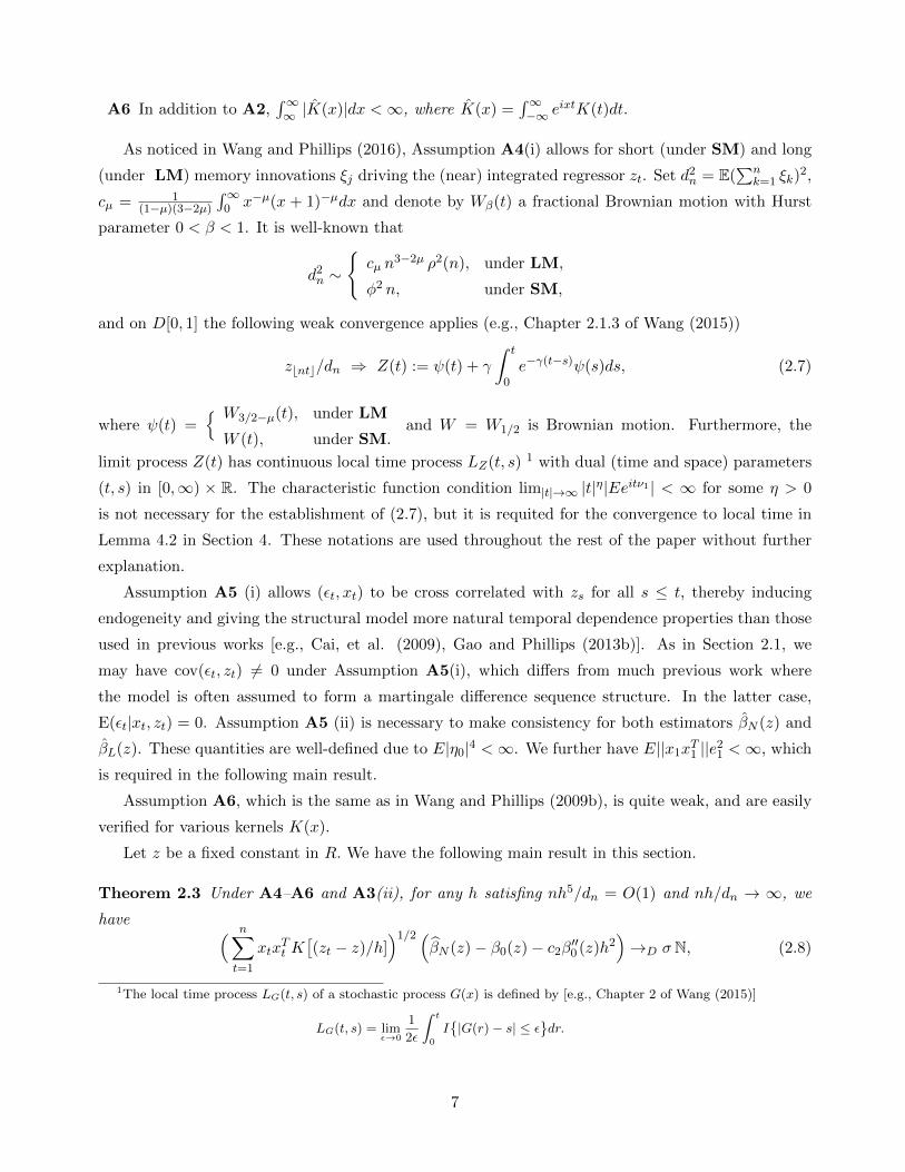
A6 In addition to A2,∫∞∞ |K(x)|dx <∞, where K(x) =

∫∞−∞ e

ixtK(t)dt.

As noticed in Wang and Phillips (2016), Assumption A4(i) allows for short (under SM) and long

(under LM) memory innovations ξj driving the (near) integrated regressor zt. Set d2n = E(

∑nk=1 ξk)

2,

cµ = 1(1−µ)(3−2µ)

∫∞0 x−µ(x + 1)−µdx and denote by Wβ(t) a fractional Brownian motion with Hurst

parameter 0 < β < 1. It is well-known that

d2n ∼

cµ n

3−2µ ρ2(n), under LM,

φ2 n, under SM,

and on D[0, 1] the following weak convergence applies (e.g., Chapter 2.1.3 of Wang (2015))

zbntc/dn ⇒ Z(t) := ψ(t) + γ

∫ t

0e−γ(t−s)ψ(s)ds, (2.7)

where ψ(t) = W3/2−µ(t), under LM

W (t), under SM.and W = W1/2 is Brownian motion. Furthermore, the

limit process Z(t) has continuous local time process LZ(t, s) 1 with dual (time and space) parameters

(t, s) in [0,∞) × R. The characteristic function condition lim|t|→∞ |t|η|Eeitν1 | < ∞ for some η > 0

is not necessary for the establishment of (2.7), but it is requited for the convergence to local time in

Lemma 4.2 in Section 4. These notations are used throughout the rest of the paper without further

explanation.

Assumption A5 (i) allows (εt, xt) to be cross correlated with zs for all s ≤ t, thereby inducing

endogeneity and giving the structural model more natural temporal dependence properties than those

used in previous works [e.g., Cai, et al. (2009), Gao and Phillips (2013b)]. As in Section 2.1, we

may have cov(εt, zt) 6= 0 under Assumption A5(i), which differs from much previous work where

the model is often assumed to form a martingale difference sequence structure. In the latter case,

E(εt|xt, zt) = 0. Assumption A5 (ii) is necessary to make consistency for both estimators βN (z) and

βL(z). These quantities are well-defined due to E|η0|4 <∞. We further have E||x1xT1 ||e2

1 <∞, which

is required in the following main result.

Assumption A6, which is the same as in Wang and Phillips (2009b), is quite weak, and are easily

verified for various kernels K(x).

Let z be a fixed constant in R. We have the following main result in this section.

Theorem 2.3 Under A4–A6 and A3(ii), for any h satisfing nh5/dn = O(1) and nh/dn → ∞, we

have ( n∑t=1

xtxTt K[(zt − z)/h]

)1/2 (βN (z)− β0(z)− c2β

′′0 (z)h2

)→D σN, (2.8)

1The local time process LG(t, s) of a stochastic process G(x) is defined by [e.g., Chapter 2 of Wang (2015)]

LG(t, s) = limε→0

1

2ε

∫ t

0

I|G(r)− s| ≤ ε

dr.

7

where c2 = 12

∫∞−∞ x

2K(x)dx, σ2 = [Ex1xT1 ]−1E(ε21x1x

T1 )∫∞−∞K

2(x)dx and N ∼ N(0, Id) is a standard

d-dimensional normal vector. Result (2.8) also holds if we replace βN (z) by βL(z).

Remark 5. In comparison with Theorem 2.2 where the result is derived under stationary zt, (2.8)

has a similar structure but with different co-variance σ2, indicating the limit distributions of βN (z),

also for βL(z), is not mutual independent. As in Theorem 2.2, the self-normalized limit (2.8) is pivotal

upon estimation of σ2, which can be constructed by

σ2 =

∑nt=1 xtx

Tt [yt − xTt βN (zt)]

2K2[(zt − z)/h]∑nt=1 xtx

Tt K[(zt − z)/h]

.

We may establish [result also holds if we replace βN (z) by βL(z)]

(nhdn

)1/2 (βN (z)− β0(z)− c2β

′′0 (z)h2

)→D τ2 L

−1/2Z (1, 0)N, (2.9)

where τ22 = [Ex1x

T1 ]−1 σ2 and N is independent of LZ(1, 0). Note that (2.9) is quite different from

(2.3) or (2.6), indicating that quite different techniques are used in establishing the results. Result

(2.9) has a slow convergence rate due to the fact that, in nonstationary case, the amount of time

spent by the process zt around any particular spatial point point z is n/dn rather than n so that the

corresponding convergence rate in such a regression is now√nh/dn. This philosophia was first noticed

in Wang and Phillips (2009a, b). Furthermore, unlike Theorem 2.2, the bias reducing advantage of

the local linear nonparametric estimator is lost under point-wise estimation as first noticed in Wang

and Phillips (2011). In contrast to point-wise estimation, the local linear non-parametric estimator

does have superior performance characteristics to the Nadaraya-Watson estimator in terms of uniform

asymptotics over wide domains (Chan and Wang, 2014; Duffy, 2017).

Remark 6. Let x1t = xt +A0, where A0 is a constant vector. Note that

Ex11ε1 = Ex1ε1 +A0Eε1 = 0.

A routine modification of Theorem 2.3 yields that result (2.8) still holds if we replace xt by x1t and

σ2 by σ21 defined by

σ21 = (A0A

T0 + Ex1x

T1 )−1E

[ε21(x1 +A0)(x1 +A0)T

] ∫ ∞−∞

K2(x)dx.

This fact indicates that Theorem 2.3 provides a natural extension of Wang and Phillips (2009b, 2016)

to a functional-coefficient cointegrating regression model. As noted in Wang and Phillips (2009b),

there is no inverse problem in structural models of nonlinear cointegration of the form (1.1) where the

regressor zt is an endogenously generated integrated process, avoiding the need for instrumentation

and completely eliminating ill-posed functional equation inversions. As a consequence, Theorem 2.3

has important implications for applications.

8

2.3 Possible extensions

In economic applications, it is important to consider multivariate extension of model (1.1), i.e., to

consider the model having the form:

yt = xTt β0(zt, wt) + εt, (2.10)

where yt, zt and εt are all scalars, xt = (xt1, · · · , xtd)T and wt = (wt1, ..., wtd1) are of dimension d and

d1, respectively, and β0(·, · · · ) is a d× 1 vector of unknown smooth function defined on R1+d1 . As in

one-dimension situation, the local kernel estimator β0(·, ·) of β0(·, ·) can be similarly defined by

β0(z, w) =

∑nt=1 xt ytK[(zt − z)/h] Πd1

j=1Kj [(wtj − wj)/hj ]∑nt=1 xt x

Tt K[(zt − z)/h]Πd1

j=1Kj [(wtj − wj)/hj ], (2.11)

where K(x),Kj(x) are non-negative kernel functions and the bandwidth h, hj ≡ hjn → 0 for j =

1, ..., d1.

If xt is nonstationary and both zt and wt are stationary, asymptotics of β0(z, w) can be obtained

by using similar arguments as in Section 2.1 under some regular settings and hence the details are

omitted. We next consider the situation that xt and wt are stationary and zt is an I(1) process.

As noticed in Section 5.1.5 of Wang (2015), to enable β0(z, w) being a consistency estimator, the

stationary assumption on wt is essentially necessary. We further assume d1 = 1 for the sake of

notation convenience. The extension to d1 ≥ 2 is straightforward.

To investigate the asymptotics of β0(z, w), as in Section 2.2, let ηi ≡ (νi, η1i, ..., ηmi)T , i ∈ Z,m ≥ 1

is a sequence of iid random vectors with Eη0 = 0, E(η0η

T0

)= Σ and E||η0||4 <∞. We also make use

of the following assumtions.

A7 [Regression function and Kernel function]

(a) The kernels K(x) and K1(x) have a common compact support Ω satisfying∫

ΩK(x)dx =∫ΩK1(x)dx = 1 and

∫∞−∞ |K(t)|dt <∞, where K(t) =

∫∞−∞ e

itxK(x)dx;

(b) When (x, y) is in a compact set, we have

|β0(x+ δ1, y + δ2)− β0(x, y)| ≤ C (|δ1|+ |δ2|), (2.12)

whenever δ1 and δ2 are sufficiently small.

A8 [Regressors]

(a) zt is defined as in A4(ii) and A4 holds;

(b) xt = (xt1, · · · , xtd)T , where xti = Γi(ηt, ..., ηt−m0+1) for some m0 > 0, where Γi(.), 1 ≤ i ≤ d,

are real measurable functions of its contents;

9

(c) wt = Γ0(ηt, ..., ηt−m0+1) for some m0 > 0, where Γ0(.) is a real measurable function of its

contents;

(d) For any fixed w and each 1 ≤ i ≤ d, E(|xti|4+δ|wt = w) <∞ with t = m0 for some δ > 0;

(e) For any fixed w and each 1 ≤ i, j ≤ d, (xti, xtj , wt) and (xti, wt) have joint density functions

pij(x, y, z) and pj(x, z), respectively, that are continuous in a neighbourhood of w;

(f) For any fixed w, Dw =(dij(w)

)1≤i,j≤d is a positive-definite matrix, where, with t = m0,

dij(w) = E(xtixtj |wt = w).

A9 [Error processes] εi,Fii≥1, where Fi+1 = σ(ηi, ηi−1, ...), is a martingale difference such that,

as i→∞, E (ε2i | Fi−1)→a.s. σ2 > 0, and, as A→∞,

supi≥1

E[ε2i I(|εi| ≥ A) | Fi−1

]= oP(1).

Theorem 2.4 Under Assumptions A7–A9, for any h and h1 satisfying nhh1/dn → ∞ and (h +

h1)2nhh1/dn → 0, we have

D1/2n

[β0(z, w)− β0(z, w)

]→D τ N, (2.13)

where Dn =∑n

t=1 xtxTt K[(zt − z)/h]K1[(wt − w)/h1] and τ2 = σ2

∫ΩK

21 (x)dx

∫ΩK

22 (x)dx, N ∼

N(0, Id) is a standard d-dimensional normal vector.

Remark 7. Theorem 2.4 provides an extension of Theorem 5.7 in Wang (2015) to a functional-

coefficient cointegrating regression model by imposing the restriction E(εt|xt, zt, wt) = 0 on the error

processes. In a related paper, Gao and Phillips (2013b) [also see Sun, et al. (2013)] investigated

the model (2.10) with both xt and zt are I(1) processes under some similar conditions. Their main

theorems made use of a result established by Phillips (2009), where the independence between xt and

zt, wt is essentially required. In terms of possible empirical applications, it is of interests to remove

these restrictions, in particular, to establish the asymptotics without imposing E(εt|xt, zt, wt) = 0 in

the model as in Theorems 2.1-2.3. There are some technical challenges in the investigation of general

model (2.10), and hence the extensions will be left for future work.

3 Conclusion

This paper studies nonparametric estimation for functional-coefficient cointegrating regression models

of the form (1.1) in two different situations: (1) xt is nonstationary and zt is stationary and (2) xt is

stationary and zt is nonstationary. Both self-normalized local kernel and local linear estimators are

shown to be asymptotic normal and to be pivotal upon an estimation of co-variances. Importantly, our

asymptotic results allow for endogenous regressor in the models, namely, we assume E(εt|xt, zt) 6= 0 in

10

(1.1). These structural models differ from various previous works and open up some interesting pos-

sibilities for functional-coefficient regression in empirical research with integrated processes. In terms

of many possible empirical applications, some extensions of the ideas presented here to other useful

models involving nonlinear functions of integrated processes seems to be interesting. In particular,

partial linear cointegration models (e.g., Gao and Phillips, 2003b)) may be treated in a similar way to

(1.1), but there are difficulties for multiple non-stationary regression models, due to the nonrecurrence

of the limit processes in high dimensions (c.f. Park and Phillips, 2001). It will also be of interest in

exploring the functional-coefficient cointegration models by the use of instrumental variables in the

present nonstationary context. We plan to report on some of these extensions in later work.

4 Proofs

Since methodology is different, the proofs of Theorems 2.1-2.2, 2.3 and 2.4 will be Sections 4.1, 4.2

and 4.3, respectively.

4.1 Proofs of Theorems 2.1 and 2.2

We start with the some preliminaries. Write xnt = xt/√n , Kj(x) = xjK(x) and µj =

∫∞−∞Kj(x)dx

for j ≥ 0. Other notation is the same as in previous sections except mentioned explicitly.

Lemma 4.1 (a) Under A1 (ii), for any 0 ≤ α ≤ 3, we have

EK[(z1 − z)/h

](1 + |ε1|α) ≤ C(z)h, (4.1)

where C(z) is a constant depending only on z; (b) Under A1 (iii), as h→ 0, we have

h−1EKj

[(z1 − z)/h

]= g(z)µj + o(1). (4.2)

The proof of Lemma 4.1 is routine, and hence the details are omitted. In the next lemma, suppose

that H(x) and H1(x) are locally bounded real functions on Rd and H1(x) satisfies the local lipschitz

condition, i.e., for any ||x||+ ||y|| ≤ K,∣∣H1(x)−H1(y)∣∣ ≤ CK ||x− y||, (4.3)

where CK is a constant depending only on K.

Lemma 4.2 (i) For any real function An(x, y),

(a) we have

1

n

n∑t=1

H(xnt)An(zt, εt) = OP(E|An(z1, ε1)|

); (4.4)

11

(b) If EAn(z1, ε1) = 0 for each n ≥ 1, then for any α > 0,

1√n

n∑t=1

H1(xnt)An(zt, εt) = OP

[E|An(z1, ε1)|2+α

]1/(2+α). (4.5)

(ii) For any h→ 0 satisfying nh1+δ →∞ for some δ > 0, we have

1

n

n∑t=1

H(xnt),1√nh

n∑t=1

H1(xnt)K[(zt − z)/h] εt

→D

∫ 1

0H(Bs)ds, a1

( ∫ 1

0H2

1 (Bs)ds)1/2

N, (4.6)

where a21 = g(z)σ2

z , N is a standard normal variate independent of Bs.

The proof of Lemma 4.2 will be given in Appendix. Note that |Kj(x)| ≤ CK(x) as K(x) has a

compact support. Result (4.4), together with (4.1), implies that, as h→ 0,

1

nh

n∑t=1

||xntxTnt|| |Kj

[(zt − z)/h

]| = OP (1). (4.7)

Similarly, by using (4.2) and (4.5) with An(zt, εt) = Kj

[(zt − z)/h

]− EKj

[(zt − z)/h

], we have

∆nj :=1

nh

n∑t=1

xntxTntKj

[(zt − z)/h

]=

1

nh

n∑t=1

xntxTntEKj

[(zt − z)/h

]+

1

nh

n∑t=1

xntxTnt

[Kj

[(zt − z)/h

]− EKj

[(zt − z)/h

]]= [g(z)µj + o(1)]

1

n

n∑t=1

xntxTnt +OP ((nh1+α/(2+α))−1/2)

= g(z)µj1

n

n∑t=1

xntxTnt + oP (1), (4.8)

by taking α sufficiently small so that nh1+α/(2+α) ≥ nh1+δ → ∞. Furthermore, it follows from (4.6)

and the continuous mapping theorem that, for any h→ 0 satisfying nh1+δ →∞ for some δ > 0,( 1

n

n∑t=1

xntxTnt,

1√nh

n∑t=1

xntK[(zt − z)/h] εt

→D

∫ 1

0BsB

Ts ds, a1

( ∫ 1

0BsB

Ts ds

)1/2 N, (4.9)

where N ∼ N(0, Id) is a d dimensional normal vector independent of Bs with covariance Id.

We are now ready to prove the main results.

Proof of Theorem 2.1. We may write

n√h(βN (z)− β0(z)− c1β

′0(z)h

)= ∆−1

n0

(Sn +Rn1 +Rn2

), (4.10)

12

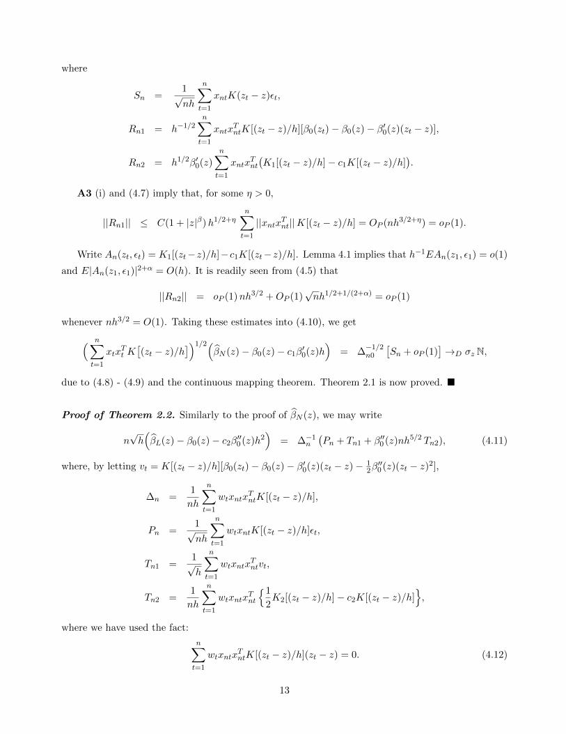
where

Sn =1√nh

n∑t=1

xntK(zt − z)εt,

Rn1 = h−1/2n∑t=1

xntxTntK[(zt − z)/h][β0(zt)− β0(z)− β′0(z)(zt − z)],

Rn2 = h1/2β′0(z)n∑t=1

xntxTnt

(K1[(zt − z)/h]− c1K[(zt − z)/h]

).

A3 (i) and (4.7) imply that, for some η > 0,

||Rn1|| ≤ C(1 + |z|β)h1/2+ηn∑t=1

||xntxTnt||K[(zt − z)/h] = OP (nh3/2+η) = oP (1).

Write An(zt, εt) = K1[(zt−z)/h]−c1K[(zt−z)/h]. Lemma 4.1 implies that h−1EAn(z1, ε1) = o(1)

and E|An(z1, ε1)|2+α = O(h). It is readily seen from (4.5) that

||Rn2|| = oP (1)nh3/2 +OP (1)√nh1/2+1/(2+α) = oP (1)

whenever nh3/2 = O(1). Taking these estimates into (4.10), we get( n∑t=1

xtxTt K[(zt − z)/h

])1/2(βN (z)− β0(z)− c1β

′0(z)h

)= ∆

−1/2n0

[Sn + oP (1)

]→D σz N,

due to (4.8) - (4.9) and the continuous mapping theorem. Theorem 2.1 is now proved.

Proof of Theorem 2.2. Similarly to the proof of βN (z), we may write

n√h(βL(z)− β0(z)− c2β

′′0 (z)h2

)= ∆−1

n

(Pn + Tn1 + β′′0 (z)nh5/2 Tn2), (4.11)

where, by letting vt = K[(zt − z)/h][β0(zt)− β0(z)− β′0(z)(zt − z)− 12β′′0 (z)(zt − z)2],

∆n =1

nh

n∑t=1

wtxntxTntK[(zt − z)/h],

Pn =1√nh

n∑t=1

wtxntK[(zt − z)/h]εt,

Tn1 =1√h

n∑t=1

wtxntxTntvt,

Tn2 =1

nh

n∑t=1

wtxntxTnt

1

2K2[(zt − z)/h]− c2K[(zt − z)/h]

,

where we have used the fact:

n∑t=1

wtxntxTntK[(zt − z)/h](zt − z) = 0. (4.12)

13

Note that, as h→ 0 and nh1+δ →∞ for some δ > 0,

n−2h1−jVnj = ∆nj = g(z)µj1

n

n∑t=1

xntxTnt + oP (1),

by (4.8). It is readily seen from (4.8) and Lemma 4.2 that, by recalling µ1 = 0 and µ0 = 1,

∆n = Vn2 ∆n0 − hVn1 ∆n1 = Vn2

[g(z)

n

n∑t=1

xntxTnt + oP (1)

];

Pn = Vn21√nh

n∑t=1

xntK[(zt − z)/h]εt − hVn11√nh

n∑t=1

xntK1[(zt − z)/h]εt

= Vn2

[ 1√nh

n∑t=1

xntK[(zt − z)/h]εt + oP (1)];

‖Tn1‖ ≤ Ch3/2+δn∑t=1

|wt| ||xntxTnt||K[(zt − z)/h]

≤ Ch3/2+δ(|Vn2|

n∑t=1

||xntxTnt||K[(zt − z)/h] + h|Vn1|n∑t=1

||xntxTnt||K1[(zt − z)/h])

= OP (nh5/2+δ)Vn2;

Tn2 = Vn21

nh

n∑t=1

xntxTnt

1

2K2[(zt − z)/h]− c2K[(zt − z)/h]

−hVn1

1

nh

n∑t=1

xntxTnt

1

2K3[(zt − z)/h]− c2K1[(zt − z)/h]

= oP (1)Vn2.

Taking these facts into (4.11), we obtain

( n∑t=1

xtxTt K[(zt − z)/h

])1/2 (βL(z)− β0(z)− c2β

′′0 (z)h2

)=

[g(z)

n

n∑t=1

xntxTnt + oP (1)

]−1/2 [ 1√nh

n∑t=1

xntK[(zt − z)/h]εt + oP (1)nh5/2]

→D σz N

as nh5/2 = O(1) and nh1+δ →∞ for some δ > 0, due to (4.9) and the continuous mapping theorem.

Theorem 2.2 is now proved.

4.2 Proof of Theorem 2.3

As in Section 4.1, let Kj(x) = xjK(x) and µj =∫∞−∞Kj(x)dx for j ≥ 0. Let

uk =

∞∑l,m=0

ϕTl ηk−l ηTk−m ϕm, (4.1)

14

where coefficient constants ϕl and ϕm are the d+ 1 dimensional vectors satisfying∑∞

l=0 l1/4‖ϕl‖ <∞

and∑∞

m=0m1/4‖ϕm‖ <∞. We start with the following lemma. The proof of Lemma 4.3 is similar to

Lemma 2.2 and Theorem 3.16 of Wang (2015). A outline will be given in the appendix. For a proof

of Lemma 4.4, we refer to Theorem 3.18 of Wang (2015). See, also, Wang and Phillips (2011).

Lemma 4.3 Let z be a fixed constant. For any 1 ≤ s, t ≤ d+ 1 and any h satisfying h log n→ 0 and

nh/dn →∞, we have

n∑k=1

(1 + |uk|)K(zk − z

h

)= OP

(nh/dn

); (4.2)

n∑k=1

(uk − Euk

)K(zk − z

h

)= OP

((nhdn

)1/2) ∞∑l,m=0

(l1/4m1/4‖ϕl‖ ‖ϕm‖

). (4.3)

and dnnh

n∑t=1

K(zt − z

h

),( dnnh

)1/2 n∑t=1

(uk − Euk

)K(zt − z

h

)→D

LZ(1, 0), a2 L

1/2Z (1, 0)N

, (4.4)

where a22 = E(u2

k)∫∞−∞K

2(t)dt, and N is standard normal variate independent of LZ(1, 0);

Lemma 4.4 Let g(x) be a real function having a compact support. If∫∞−∞ g(x)dx = 0, then

n∑k=1

g(zk − z

h

)= OP

((nh/dn

)1/2), (4.5)

for any h satisfying nh/dn →∞.

Since, due to Assumption A5, each element of xtxTt and xtεt can be representated as uk for some

specified ϕl and ϕm, it follows from Lemma 4.3 that

Dnj :=dnnh

n∑t=1

xtxTt Kj

(zt − zh

)=

dnnh

n∑t=1

E(xtxTt )Kj

(zt − zh

)+dnnh

n∑t=1

[xtx

Tt − E(xtx

Tt )]Kj

(zt − zh

)= E(x1x

T1 )dnnh

n∑t=1

Kj

(zt − zh

)+OP

(( dnnh

)1/2)= E(x1x

T1 )dnnh

n∑t=1

Kj

(zt − zh

)+ oP (1), (4.6)

as nh/dn → ∞. Furthermore, due to E(x1ε1) = 0, it follows from (4.4) and the continuous mapping

theorem that dnnh

n∑t=1

K(zt − z

h

),( dnnh

)1/2 n∑t=1

xtεtK(zt − z

h

)15

→D

LZ(1, 0), a2 L

1/2Z (1, 0)N

, (4.7)

where a22 = E(ε21x1x

T1 )∫∞−∞K

2(x)dx, and N ∼ N(0, Id) is a d dimensional normal vector independent

of LZ(1, 0).

We are now ready to prove Theorems 2.3. By letting vt = K(zt−zh

)[β0(zt)−β0(z)−β′0(z)(zt− z)−

12β′′0 (z)(zt − z)2], we may write(nh

dn

)1/2(βN (z)− β0(z)− c2β

′′0 (z)h2

)= D−1

n0

(Sn +Rn1 + β′0(z)Rn2 + β′′0 (z)Rn3

), (4.8)

where

Sn =( dnnh

)1/2 n∑t=1

xtεtK(zt − z

h

),

Rn1 =( dnnh

)1/2 n∑t=1

xtxTt vt,

Rn2 = h( dnnh

)1/2 n∑t=1

xtxTt K1

(zt − zh

),

Rn3 = h2( dnnh

)1/2 n∑t=1

xtxTt

1

2K2[(zt − z)/h]− c2K[(zt − z)/h]

.

From A3(ii) and (4.2), as nh5/dn = O(1) we have

‖Rn1‖ ≤ Ch2+η( dnnh

)1/2n∑t=1

||xtxTt ||K(zt − z

h

)= OP

((nhdn

)1/2h2+η

)= oP (1). (4.9)

From (4.3) and (4.5), as h→ 0 we have

Rn2 = h( dnnh

)1/2 n∑t=1

[xtx

Tt − E(xtx

Tt )]K1

(zt − zh

)+h

( dnnh

)1/2 n∑t=1

E(xtxTt )K1

(zt − zh

)= OP (h) = oP (1). (4.10)

Note that∫∞−∞

[12K2(x)−c2K(x)

]dx = 0. It follows from (4.3) and (4.5) again that, as nh5/dn = O(1),

Rn3 = h2( dnnh

)1/2 n∑t=1

[xtx

Tt − E(xtx

Tt )]1

2K2[(zt − z)/h]− c2K[(zt − z)/h]

+(nh5

dn

)1/2 dnnh

n∑t=1

E(xtxTt )1

2K2[(zt − z)/h]− c2K[(zt − z)/h]

= OP (h2) +Op

((nh5/dn

)1/2)oP (1) = oP (1). (4.11)

Combining (4.6) and (4.8)-(4.11), we obtain( n∑t=1

xtxTt K[(zt − z)/h]

)1/2 (βN (z)− β0(z)− c2β

′′0 (z)h2

)16

=[E(x1x

T1 )dnnh

n∑t=1

K(zt − z

h

)+ oP (1)

]−1/2 [( dnnh

)1/2 n∑t=1

xtεtK(zt − z

h

)+ oP (1)

]→D σN,

due to (4.7) and the continuous mapping theorem. This proves (2.8).

We next prove that(2.8) still holds if βN (z) is replaced by βL(z). In fact, as in the proof of Theorem

2.2, we may write(nhdn

)1/2(βL(z)− β0(z)− c2β

′′0 (z)h2

)= D−1

n

(Pn + Tn1 + β′′0 (z)Tn2

), (4.12)

by virtue of (4.12), where

Dn =dnnh

n∑t=1

wtxtxTt K(zt − z

h

),

Pn =( dnnh

)1/2 n∑t=1

wtxtεtK(zt − z

h

),

Tn1 =( dnnh

)1/2 n∑t=1

wtxtxTt vt,

Tn2 = h2( dnnh

)1/2 n∑t=1

wtxtxTt

1

2K2[(zt − z)/h]− c2K[(zt − z)/h]

.

Noting that from (4.6), it can be obtained

dnnhh−jVnj = Dnj = E(x1x

T1 )dnnh

n∑t=1

Kj

(zt − zh

)+ oP (1).

Since µ1 = 0 and µ0 = 1, from Lemmas 4.3 and 4.4 we have

Dn = Vn2Dn0 − hVn1Dn1 = Vn2[Dn0 + oP (1)];

Pn = Vn2

( dnnh

)1/2n∑t=1

xtεtK(zt − z

h

)− hVn1

( dnnh

)1/2n∑t=1

xtεtK1

(zt − zh

)= Vn2

[( dnnh

)1/2n∑t=1

xtεtK(zt − z

h

)+ oP (1)

];

‖Tn1‖ ≤ Vn2‖Rn1‖+ h|Vn1|n∑t=1

xtxTt |vt(zt − z)|

= OP

((nh

dn)1/2 h2+η

)Vn2;

Tn2 = Vn2Rn3 − Vn1 h3( dnnh

)1/2n∑t=1

xtxTt

1

2K3[(zt − z)/h]− c2K1[(zt − z)/h]

= oP (1)Vn2.

Taking these facts into (4.12), the claim follows from( n∑t=1

xtxTt K[(zt − z)/h

])1/2 (βL(z)− β0(z)− c2β

′′0 (z)h2

)17

=[E(x1x

T1 )dnnh

n∑t=1

K(zt − z

h

)+ oP (1)

]−1/2 [( dnnh

)1/2n∑t=1

xtεtK(zt − z

h

)+ oP (1)

]→D σN,

due to (4.7) and the continuous mapping theorem. Theorem 2.3 is now proved.

4.3 Proof of Theorem 2.4

Let Vt = xtK[(zt − z)/h]K1[(wt − w)/h1]. We may write

D1/2n

[β0(z, w)− β0(z, w)

]= D−1/2

n Sn +Rn. (4.13)

where Sn =∑n

t=1 εt Vt and, by (2.12),

||Rn|| =n∑t=1

|β0(zt, wt)− β0(z, w)| ||D−1/2n Vt||

≤ C(|h1|+ |h2|)n∑t=1

||D−1/2n Vt||.

By the continuous mapping theorem, result (2.13) will follow if we prove

||Rn|| = oP (1), (4.14)

and for any A = (A1, ..., Ad)T ∈ Rd, dn

nhh1ATDnA,

( dnnhh1

)1/2ATSn

→D

(ATDwA)LZ(1, 0), τ1/2 (ATDwA)N L

1/2Z (1, 0)

, (4.15)

where LZ((1, 0) is given as in Section 2.2 and N ∼ N(0, 1) is independent of LZ(1, 0).

We start with some preliminaries. Set ∆t =∑d

k,j=1AkAjxtkxtjK1[(wt − w)/h1]. Since, by A8(d)

and some standard arguments,

ExtixtjKγ1 [(wt − w)/h1] = h1E(xtixtj |wt = w)

∫ΩKγ

1 (x)dx+ o(h1),

E|xti|βKγ1 [(wt − w)/h1] = h1E(|xti|β|wt = w)

∫ΩKγ

1 (x)dx+ o(h1) = O(h1),

for any γ > 0, 0 ≤ β ≤ 4 + δ and uniformly for all t ≥ m0, we have E∆t = h1[ATDA + o(1)] and

E∆2t = O(h1). Now it follows from Lemma 2.2 (ii) of Wang (2015) that, for any A = (A1, ..., Ad)

T ∈ Rd,

dnnhh1

ATDnA =dnnhh1

n∑t=1

K[(zt − z)/h]E∆t +dnnhh1

n∑t=1

K[(zt − z)/h] (∆t − E∆t)

=[ATDwA+ o(1)

] dnnh

n∑t=1

K[(zt − z)/h] +OP[(dnnhh1

)1/2]

18

=[ATDwA+ o(1)

] dnnh

n∑t=1

K[(zt − z)/h] + oP (1), (4.16)

due to nhh1/dn →∞. Similarly, we have

dnnhh1

n∑t=1

(ATVt)2 =

[ATDwA+ o(1)

] ∫ΩK2

1 (x)dxdnnh

n∑t=1

K2[(zt − z)/h]

+oP (1), (4.17)

and

n∑t=1

(||Vt||+ ||Vt||2+δ/2

)=

n∑t=1

(||xt||+ ||xt||2+δ)K[(zt − z)/h]K1[(wt − w)/h1]

≤ O(h1)n∑t=1

K[(zt − z)/h] +OP [(nhh1/dn)1/2]

= OP (nhh1/dn), (4.18)

where we have used the fact that∑n

t=1K[(zt − z)/h] = OP (nh/dn). By virtue of Theorem 2.21 of

Wang (2015), results (4.16)-(4.17) imply that

∑[nt]j=1 νj√n

,

∑[nt]j=1 ν−j√n

,dnnhh1

ATDnA,dnnhh1

n∑t=1

(ATVt)2

⇒Bt, B−t, (ATDwA)LZ(1, 0), τ1 (ATDwA)LZ(1, 0)

, (4.19)

on DR4 [0,∞), where B = Btt∈R is a standard Brown motion and

τ1 =

∫ΩK2

1 (x)dx

∫ΩK2(x)dx.

We are now ready to prove (4.14) and (4.15). By noting that Dw is positive-definite, it is readily

seen from (4.16) that D−1n = OP (dn/nhh1). This, together with (4.18), yields that

||Rn|| = (|h|+ |h1|)OP [(dn/nhh1)1/2]n∑t=1

||Vt|| = OP[(|h|+ |h1|) (nhh1/dn)1/2

]= oP (1),

implying (4.14).

To prove (4.15), write unt =(dnnhh1

)1/2ATVt, namely, we have

(dnnhh1

)1/2ATSn =

∑nt=1 εt unt. By

using (4.16), routine calculations show that 1√n

∑nt=1 |unt| = oP (1) and

max1≤t≤n

|unt| ≤( dnnhh1

)1+δ/4n∑t=1

|ATVt|2+δ/2 = oP (1).

Now, by recalling A8 and (4.19), (4.15) follows from Wang’s extended martingale limit theorem, e.g.,

Wang (2014 or Theorem 3.14 of Wang (2015) . The proof of Theorem 2.4 is complete.

19

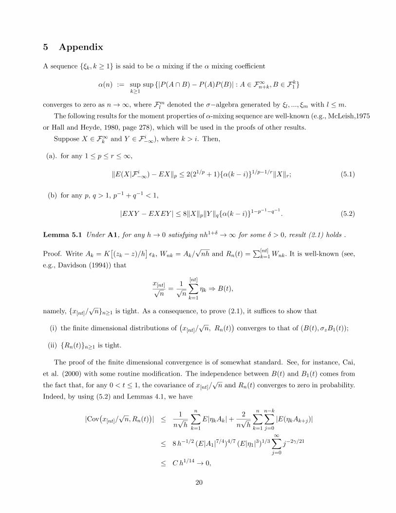
5 Appendix

A sequence ξk, k ≥ 1 is said to be α mixing if the α mixing coefficient

α(n) := supk≥1

sup |P (A ∩B)− P (A)P (B)| : A ∈ F∞n+k, B ∈ Fk1

converges to zero as n→∞, where Fml denoted the σ−algebra generated by ξl, ..., ξm with l ≤ m.

The following results for the moment properties of α-mixing sequence are well-known (e.g., McLeish,1975

or Hall and Heyde, 1980, page 278), which will be used in the proofs of other results.

Suppose X ∈ F∞k and Y ∈ F i−∞), where k > i. Then,

(a). for any 1 ≤ p ≤ r ≤ ∞,

‖E(X|F i−∞)− EX‖p ≤ 2(21/p + 1)α(k − i)1/p−1/r‖X‖r; (5.1)

(b) for any p, q > 1, p−1 + q−1 < 1,

|EXY − EXEY | ≤ 8‖X‖p‖Y ‖qα(k − i)1−p−1−q−1. (5.2)

Lemma 5.1 Under A1, for any h→ 0 satisfying nh1+δ →∞ for some δ > 0, result (2.1) holds .

Proof. Write Ak = K[(zk − z)/h

]εk, Wnk = Ak/

√nh and Rn(t) =

∑[nt]k=1Wnk. It is well-known (see,

e.g., Davidson (1994)) that

x[nt]√n

=1√n

[nt]∑k=1

ηk ⇒ B(t),

namely, x[nt]/√nn≥1 is tight. As a consequence, to prove (2.1), it suffices to show that

(i) the finite dimensional distributions of(x[nt]/

√n, Rn(t)

)converges to that of (B(t), σzB1(t));

(ii) Rn(t)n≥1 is tight.

The proof of the finite dimensional convergence is of somewhat standard. See, for instance, Cai,

et al. (2000) with some routine modification. The independence between B(t) and B1(t) comes from

the fact that, for any 0 < t ≤ 1, the covariance of x[nt]/√n and Rn(t) converges to zero in probability.

Indeed, by using (5.2) and Lemmas 4.1, we have

|Cov(x[nt]/

√n,Rn(t)

)| ≤ 1

n√h

n∑k=1

E|ηkAk|+2

n√h

n∑k=1

n−k∑j=0

|E(ηkAk+j)|

≤ 8h−1/2 (E|A1|7/4)4/7 (E|η1|3)1/3∞∑j=0

j−2γ/21

≤ C h1/14 → 0,

20

for any 0 < t ≤ 1 and γ > 21/2. Simple calculations by using similar arguments [see, e.g., Lemma A1

(c) of Cai, et al. (2000)] also yield that

supn≥1

ER2n(t) ≤ C t, (5.3)

indicating that Rn(t)n≥1, for any 0 < t ≤ 1, is uniformly integrable. This fact will be used later.

We next prove the tightness. To this end, let Fk = σ(zi, εi; i ≤ k),

βnk =

∞∑i=1

E(Wn,i+k|Fk), wnk =

∞∑i=0

[E(Wn,i+k|Fk)− E(Wn,i+k|Fk−1)

It is well-known that βnk and wnk are well defined and Wnk = wnk + βn,k−1 − βnk. Since Rn(t) =∑[nt]k=1wnk + βn,[nt], the tightness of Rn(t) will follow if we prove that

∑[nt]k=1wnk is tight and

E max1≤k≤n

|βnk| = oP (1). (5.4)

Note that wnk,Fk forms a sequence of martingale differences and the finite dimensional distribution

converges to a joint normal distribution. To prove∑[nt]

k=1wnk is tight, it suffice to show that, for any

t > 0,∑[nt]

k=1wnk is uniformly integrable [see, e.g., Proposition 1.2 of Aldous (1989)], which follows

from (5.3), (5.4) and the fact Rn(t) =∑[nt]

k=1wnk + βn,nt again.

It remains to prove (5.4). Note that EA1 = 0 and E|A1|r ≤ C(z)h for any 1 ≤ r ≤ 3 by (4.1).

Standard arguments by using (5.1), together with α(n) = O(n−γ) for some γ > 0, show that, for any

1 ≤ p < 3 and 0 < α ≤ 3− p,(E|E(Ai+k|Fi)|p

)1/p≤ Cα(k)α/p(p+α)

(E|A1|p+α

)1/(p+α)

and

(E|βni|p)1/p ≤ (nh)−1/2∞∑k=1

(E|E(Ai+k|Fi)|p

)1/p ≤ C (nh)−1/2 h1/(p+α)∞∑k=1

k−γα/p(p+α). (5.5)

This implies that, for any 2 < p < 3, 0 < α ≤ 3− p and γα/p(p+ α) > 1,

E max1≤k≤n

|βnk| ≤[ n∑i=1

E|βni|p]1/p≤ C

(nh1+α/[(p+α)(p/2−1)]

)(1−p/2)/p.

We now establish (5.4) by taking γ > 6/δ, and α sufficiently small so that

nh1+α/[(p+α)(p/2−1)] ≥ nh1+δ →∞.

The proof of Lemma 5.1 is now complete.

Proof of Lemma 4.2. We only prove (4.6). Due to the local boundedness of H(x), (4.4) is obvious.

The proof of (4.5) follows from similar arguments as in proof of (4.6). We omit the details.

21

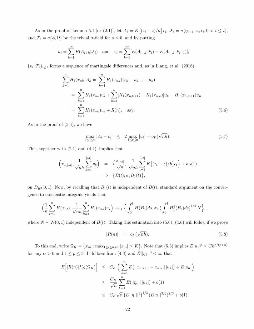
As in the proof of Lemma 5.1 [or (2.1)], let Ai = K[(zi − z)/h

]εi, Ft = σ(ηi+1, zi, εi, 0 < i ≤ t),

and Fs = σ(φ,Ω) be the trivial σ-field for s ≤ 0, and by putting

ui =∞∑k=1

E(Ai+k|Fi) and vi =∞∑k=0

[E(Ai+k|Fi)− E(Ai+k|Fi−1)],

vi,Fii≥1 forms a sequence of martingale differences and, as in Liang, et al. (2016),

n∑k=1

H1(xnk)Ak =

n∑k=1

H1(xnk)(vk + uk−1 − uk)

=

n∑k=1

H1(xnk)vk +

n∑k=1

[H1(xn,k+1)−H1(xn,k)]uk −H1(xn,n+1)un

=

n∑k=1

H1(xnk)vk +R(n), say. (5.6)

As in the proof of (5.4), we have

max1≤i≤n

|Ai − vi| ≤ 2 max1≤i≤n

|ui| = oP (√nh). (5.7)

This, together with (2.1) and (4.4), implies that

(xn,[nt],

1√nh

[nt]∑k=1

vk

)=

x[nt]√n,

1√nh

[nt]∑t=1

K[(zt − z)/h

]εt

+ oP (1)

⇒B(t), σzB1(t)

,

on DR2 [0, 1]. Now, by recalling that B1(t) is independent of B(t), standard argument on the conver-

gence to stochastic integrals yields that( 1

n

n∑t=1

H(xnt),1√nh

n∑k=1

H1(xnk)vk

)→D

∫ 1

0H(Bs)ds, σz

( ∫ 1

0H2

1 (Bs)ds)1/2

N,

where N ∼ N(0, 1) independent of B(t). Taking this estimation into (5.6), (4.6) will follow if we prove

|R(n)| = oP (√nh). (5.8)

To this end, write ΩK = xni : max1≤i≤n+1 |xni| ≤ K. Note that (5.5) implies E|u1|p ≤ Chp/(p+α)

for any α > 0 and 1 ≤ p ≤ 3. It follows from (4.3) and E||η1||3 <∞ that

E[|R(n)|I(g(ΩK)

]≤ CK

( n∑k=1

E(||xn,k+1 − xn,k|| |uk|

)+ E|un|

)≤ CK√

n

n∑k=1

E(||ηk|| |uk|) + o(1)

≤ CK√n(E||η1||3

)1/3(E|u1|3/2)2/3 + o(1)

22

≤ CK√nh2/(3+2α) + o(1) = o(

√nh),

by taking α < 1/2. This implies that R(n) = oP (√nh) due to P (ΩK)→ 1 as K →∞.

The proof of Lemma 4.2 is complete.

Proof of Lemma 4.3. We only provide a outline. Results (4.2) and (4.5) follow from (2.94) and

Theorem 3.18 of Wang (2015), respectively. By using similar arguments as in proof of (2.96) in Wang

(2015), for any l,m ≥ 0, we have

E( n∑k=1

[ηk−lη

Tk−m − E(ηk−lη

Tk−m)

]K[(zk − z)/h]

)2

≤ C (1 + maxl1/2,m1/2+ h log n)[E(η1η

T1 ) + E(η1η

T2 )]nh/dn.

This, together with Holder’s inequality, yields that

E∣∣∣ n∑k=1

(uk − Euk)K(zk − z

h

)∣∣∣≤

∞∑l,m=0

‖ϕl‖ ‖ϕm‖E∣∣∣ n∑k=1

[ηk−lη

Tk−m − E(ηk−lη

Tk−m)

]K[(zk − z)/h]

∣∣∣= O

[(nh/dn

)1/2] ∞∑l,m=0

(l1/4m1/4‖ϕl‖ ‖ϕm‖

),

implying (4.3). To see (4.4), let ukM =∑M

l,m=0 ϕTl ηk−l η

Tk−m ϕm and uk = uk − Euk, ukM = ukM −

EukM . For any M ≥ 1, (3.8) of Wang and Phillips (2009b) implies that dnnh

n∑t=1

K(zt − z

h

),( dnnh

)1/2 n∑t=1

ukM K(zt − z

h

)→D

LZ(1, 0), aM2 L

1/2Z (1, 0)N

, (5.9)

where a2M2 = E(u2

kM )∫∞−∞K

2(t)dt. Since a2M2 → a2

2 as M → ∞, (4.4) follows easily from (5.9) and

the fact: ( dnnh

)1/2 n∑k=1

(uk − ukM

)K(zt − z

h

)= OP (1)

( ∞∑l=M,m=0

+∞∑

l=0,m=M

)l1/4m1/4‖ϕl‖ ‖ϕm‖ = oP (1),

as n→∞ first and then M →∞. The proof of Lemma 4.3 is now complete.

Acknowledgments. Liang acknowledges research support from the National Natural Science Foun-

dation of China (11671299). Shen acknowledges research support from the international exchange

program for graduate students, Tongji University (2016020028). Wang acknowledges research support

from the Australian Research Council.

23

References

[1] Aldous, D.J. (1989). Stopping times and tightness, II, Ann. Probab. 17, 586-595.

[2] Cai, Z., Li, Q. and Park, J.Y. (2009). Functional-coefficient models for nonstationary time series

data. Journal of Econometrics 148, 101-113.

[3] Cai, Z., Fan, J. and Yao, Q. (2000). Functional-coefficient regression models for nonlinear time

series, Journal of Amer. Assoc., 95, 941-956.

[4] Chan, N. and Wang, Q. (2014). Uniform convergence for nonparametric estimators with non-

stationary data. Econometric Theory, 30, 1110-1133.

[5] Chan, N. and Wang, Q. (2015) Nonlinear regressions with nonstationary time series. Journal of

Econometrics 185(1), 182-195.

[6] Chang, Y. and Park, J.Y. (2003) Index models with integrated time series. Journal of Econo-

metrics 114(1), 73-106.

[7] Chang, Y., Park, J.Y. and Phillips, P.C.B. (2001). Nonlinear econometric models with cointe-

grated and deterministically trending regressors. Econometrics Journal 4, 1-36.

[8] Davidson, J. (1994). Stochastic Limit Theory, Oxford University Press.

[9] Duffy, J. (2017). Uniform convergence rates on a maximal domain for structural nonparametric

cointegrating regression. Econometrics Journal , forthcoming.

[10] Engle, R.F. and Granger, C.W.J. (1987). Cointegration and error correction: Representation,

estimation, and testing. Econometrica 55, 251-276.

[11] Fan, J. and Gijbels, I. (1996). Local Polynomial Modeling and its Applications. Chapman and

Hall, London.

[12] Gao, J. and Phillips, P.C.B. (2013a). Semiparametric estimation in triangular system equations

with nonstationarity, Journal of Econometrics, 176, 59–79.

[13] Gao, J. and Phillips, P.C.B. (2013b). Functional coefficient nonstationary regression. Cowles

fundation discussion paper No 1911.

[14] Granger, C.W.J. (1981). Some properties of time series data and their use in econometric model

specification. Journal of Econometrics 16, 121-130.

[15] Hall, P. and Heyde, C.C. (1980). Martingale Limit Theory and its Application. Academic Press.

[16] Li, K. Li, D. Liang, Z and Hsiao, C. (2017). Estimation of semi-varying coefficient models with

nonstationary regressors. Econometric Review, 36, 354–369.

24

[17] Liang H.-Y., Phillips, P.C.B., Wang, H. and Wang, Q. (2016). Weak convergence to stochastic

integrals for econometric applications. Econometric Theory 32, 1349-1375.

[18] McLeish, D.L. (1975) A maximal inequality and dependent strong laws. Annals of Probability

3, 829-839.

[19] Park, J.Y. and Phillips, P.C.B. (1988). Statistical inference in regressions with integrated pro-

cesses: Part 1. Econometric Theory 4, 468-497.

[20] Park, J.Y. and Phillips, P.C.B. (2001). Nonlinear regressions with integrated time series. Econo-

metrica 69, 117-161.

[21] Phillips, P.C.B (2009). Local Limit theorem and spurious regressions, Econometric Theory, 15,

269-298.

[22] Sun, Y. Cai, Z and Li, Q. (2013). Semiparametric functional coefficient models with integrated

covariaates, Econometric Theory, 29, 659–672.

[23] Saikkonen P. (1995). Problems with the asymptotic theory of maximum likelihood estimation

in integrated and cointegrated systems. Econometric Theory 11(5), 888-911.

[24] Terasvirta, T. Tjostheim, D. and Granger, C. W. J. (2011). Modelling nonlinear economic time

series, Oxford University Press.

[25] Trokic, M. (2014). Functional Coefficient Models for Nearly (Possibly Weakly) I(1) Processe,

online, https : //papers.ssrn.com/sol3/papers.cfm?abstractid = 2374495.

[26] Wang, Q. (2014). Martingale limit theorems revisited and non-linear cointegrating regression.

Econometric Theory, 30, 509-535.

[27] Wang, Q. (2015). Limit Theorems for Nonlinear Cointegrating Regression. World Scientific.

[28] Wang, Q. and Phillips, P.C.B. (2009a) Asymptotic theory for local time density estimation and

nonparametric cointegrating regression. Econometric Theory 25, 710-738.

[29] Wang, Q. and Phillips, P.C.B. (2009b). Structural Nonparametric Cointegrating Regression,

Econometrica, 25, 1901-1948.

[30] Wang, Q. and Phillips, P. C. B. (2011). Asymptotic Theory for Zero Energy Functionals with

Nonparametric Regression Applications. Econometric Theory, 27, 235-259.

[31] Wang, Q. and Phillips, P.C. B.(2016). Nonparametric cointegrating regression with endogeneity

and long memory. Econometric Theory, 32, 359–401.

[32] Xiao, Z. (2009). Functional-coefficient cointegration models. Journal of Econometrics 152, 81-92.

25