Discrete Applied Mathematics 144 (2004) 231–236www.elsevier.com/locate/dam

Fun-Sort—or the chaos of unordered binary search

Therese Biedla, Timothy Chana, Erik D. Demaineb, Rudolf Fleischerc;1,Mordecai Golinc, James A. Kinga, J. Ian Munroa

aDepartment of Computer Science, University of Waterloo, Waterloo, ON, Canada N2L 3G1bMIT Laboratory for Computer Science, Cambridge, MA 02139, USA

cDepartment of Computer Science, The Hong Kong University of Science and Technology, Clear Water Bay, Kowloon,Hong Kong

Received 30 April 2002; received in revised form 15 December 2003; accepted 22 January 2004

Abstract

Usually, binary search only makes sense in sorted arrays. We show that insertion sort based on repeated “binarysearches” in an initially unsorted array also sorts n elements in time 9(n2 log n). If n is a power of two, then the expectedtermination point of a binary search in a random permutation of n elements is exactly the cell where the element shouldbe if the array was sorted. We further show that we can sort in expected time 9(n2 log n) by always picking two randomcells and swapping their contents if they are not ordered correctly.c© 2004 Elsevier B.V. All rights reserved.

Keywords: Oblivious sorting; Insertion-sort; Binary search

1. Introduction

Comparison-based sorting algorithms apply four paradigms: selection, insertion, exchanging, and merging [3, p. 73].Most methods operate by maintaining an invariant (of sortedness) on an increasingly longer segment of the array or, asin the case of Quicksort, at least strong invariants on the progress made thus far. Shellsort, from one point of view,maintains sorted subarrays of increasingly greater length as the process continues. From another point of view, Shellsortis delightfully chaotic. At any stage, one is presented with a subsequence which one hopes is reasonably close to sorted,and then one is to complete the task by using linear Insertion-Sort.

We study exchange sorting algorithms, i.e., algorithms that compare pairs of array elements and swap them if theyare out of order. In particular, we consider the algorithm Fun-Sort 2 that repeatedly moves values from current to “morelikely” locations by performing a “binary search”. Since the array is initially unsorted, a “binary search” will most likelyend up at the wrong array position, resulting in rather chaotic behavior of the insertion sort algorithm. Nevertheless, wewere able to adapt the method to correctly perform a sort in the (rather poor) worst-case runtime by 9(n2 log n). However,we feel the greater contribution of this paper is to lay open the approach, both for purposes of algorithmic improvementsand for improvements in the expected runtime of our approach. In particular, we observe that in a randomly permutedarray a “binary search” for an element of rank i will on the average end at position i. We also ask whether the paradigmcan be further developed to give substantially better behavior in the worst case.

1 R. Fleischer was partially supported by HKUST grant DAG00/01.EG03.E-mail addresses: biedl@uwaterloo.ca (T. Biedl), tmchan@uwaterloo.ca (T. Chan), edemaine@mit.edu (E.D. Demaine),

rudolf@cs.ust.hk (R. Fleischer), golin@cs.ust.hk (M. Golin), ja3king@uwaterloo.ca (J.A. King), imunro@uwaterloo.ca (J. I. Munro).2 After the conference series Fun with Algorithms.

0166-218X/$ - see front matter c© 2004 Elsevier B.V. All rights reserved.doi:10.1016/j.dam.2004.01.003

232 T. Biedl et al. / Discrete Applied Mathematics 144 (2004) 231–236

This paper is organized as follows. In Section 2 we deJne the model of exchange sorting algorithms. In Section 3 weintroduce Guess-Sort, a simple randomized exchange sorting algorithm which runs in expected time O(n2 log n). We alsogive a new direct proof of an old theorem that n − 1 rounds of comparing all adjacent cells, in any order, suKce tosort. In Section 4 we show that Fun-Sort, which is Insertion-Sort where insertions are guided by “binary search” in theinitially unsorted array, sorts in time O(n2 log n). We conclude with a few open problems in Section 5.

2. Basics

Let an array a hold n elements from a totally ordered set. When convenient, we will assume that these elements aredistinct; all results also hold in general. Denote the contents of cell i by ai, for i = 1; : : : ; n. Our goal is to sort theseelements in non-decreasing order. In an exchange sorting algorithm we concentrate on just two elements at a time, fromwhich we can extract only one bit of information. A pair (i; j) of cells i and j, where i �= j, is good if the cell contents arecorrectly ordered, i.e., ai ¡aj if i ¡ j, or ai ¿aj if i ¿ j. Otherwise the pair is bad. Bad pairs are also called inversions.The number of inversions in the array is between zero if the array is correctly sorted, and ( n2 ) if the array is sorted inreverse order.

Sorting algorithms based on Jnding and swapping bad pairs are called exchange sorting algorithms [3, p. 73]. Aprimitive comparison compares two adjacent cells. A primitive exchange sorting algorithm only does primitive compar-isons. In an oblivious sorting algorithm the sequence of comparisons is Jxed in advance, i.e., it is independent of theinput sequence or the outcome of individual comparisons. Bubblesort is an example of an oblivious primitive exchangesorting algorithm.

De Bruijn showed that adding arbitrary comparisons to an oblivious primitive sorting algorithm yields another sortingalgorithm. As a consequence (also attributed to de Bruijn by some authors [7, Fact 1]; [5, Proposition 1.9], although hispaper does not mention this corollary) we see that doing n rounds of all n− 1 primitive comparisons, in arbitrary order,is already an oblivious primitive sorting algorithm (because the n phases of Odd–Even Transposition Sort [3, p. 240]can be found in the augmented sorting algorithm). Later, de Bruijn’s theorem was rediscovered [8,4,1] and the corollarywas slightly improved; it was shown that n− 1 rounds of all primitive comparisons are suKcient to sort. In Section 3 wegive a new direct proof without reducing to Odd–Even Transposition Sort. Note that the bound of n− 1 rounds is tight.If we want to sort the input sequence 1; 0; : : : ; 0 by repeatedly comparing the pairs (n − 1; n); (n − 2; n − 1); : : : ; (1; 2) inthis order then we need n− 1 rounds to move the ‘1’ to the rightmost position.

The following simple observation is folklore and implies that we can sort by repeatedly swapping bad pairs.

Lemma 1. Swapping a bad pair strictly decreases the number of inversions.

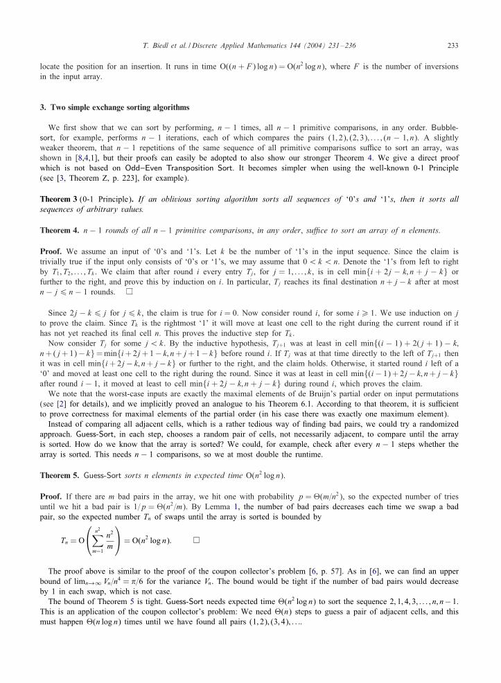
Proof. Consider swapping a bad pair (i; j), where i ¡ j and ai ¿aj (see Fig. 1). Let (k; ‘) be a good pair before theswap, where k ¡‘. Since cell i becomes smaller and cell j becomes larger, (k; ‘) can only turn bad if k= j or ‘= i.

In the former case, (i; ‘) was a bad pair before the swap (because ai moves to cell j) but it is good afterwards; in thelatter case, (k; j) was a bad pair before the swap (because aj moves to cell i) but it is good afterwards. In any case, thenumber of bad pairs decreases because (i; j) becomes a good pair.

Corollary 2. Any exchange sorting algorithm terminates after swapping at most ( n2 ) = O(n2) bad pairs.

If we could somehow identify the indices of bad pairs we could sort in O(n2) time. Unfortunately, we cannot expectto get this information for free. In Section 3 we show that choosing the comparisons randomly yields a sorting algorithmwith expected running time O(n2 log n). In Section 4 we use “binary search” (in an initially unordered array) to Jnd badpairs in logarithmic time. The resulting algorithm can be seen as Insertion-Sort based on “unordered binary searches” to

Fig. 1. If we swap the bad pair (i; j) then the good pair (k; ‘) becomes a bad pair. However, the bad pair (i; ‘) becomes a good pair.As an unintended (but pleasant) side eRect, we also turn the bad pairs (i; m) and (m; j) into good pairs.

T. Biedl et al. / Discrete Applied Mathematics 144 (2004) 231–236 233

locate the position for an insertion. It runs in time O((n + F) log n) = O(n2 log n), where F is the number of inversionsin the input array.

3. Two simple exchange sorting algorithms

We Jrst show that we can sort by performing, n − 1 times, all n − 1 primitive comparisons, in any order. Bubble-sort, for example, performs n − 1 iterations, each of which compares the pairs (1; 2); (2; 3); : : : ; (n − 1; n). A slightlyweaker theorem, that n − 1 repetitions of the same sequence of all primitive comparisons suKce to sort an array, wasshown in [8,4,1], but their proofs can easily be adopted to also show our stronger Theorem 4. We give a direct proofwhich is not based on Odd–Even Transposition Sort. It becomes simpler when using the well-known 0-1 Principle(see [3, Theorem Z, p. 223], for example).

Theorem 3 (0-1 Principle). If an oblivious sorting algorithm sorts all sequences of ‘0’s and ‘1’s, then it sorts allsequences of arbitrary values.

Theorem 4. n− 1 rounds of all n− 1 primitive comparisons, in any order, su9ce to sort an array of n elements.

Proof. We assume an input of ‘0’s and ‘1’s. Let k be the number of ‘1’s in the input sequence. Since the claim istrivially true if the input only consists of ‘0’s or ‘1’s, we may assume that 0¡k¡n. Denote the ‘1’s from left to rightby T1; T2; : : : ; Tk . We claim that after round i every entry Tj , for j = 1; : : : ; k, is in cell min{i + 2j − k; n + j − k} orfurther to the right, and prove this by induction on i. In particular, Tj reaches its Jnal destination n+ j− k after at mostn− j6 n− 1 rounds.

Since 2j − k6 j for j6 k, the claim is true for i = 0. Now consider round i, for some i¿ 1. We use induction on jto prove the claim. Since Tk is the rightmost ‘1’ it will move at least one cell to the right during the current round if ithas not yet reached its Jnal cell n. This proves the inductive step for Tk .

Now consider Tj for some j¡ k. By the inductive hypothesis, Tj+1 was at least in cell min{(i − 1) + 2(j + 1) − k;n+ (j+ 1) − k} = min{i+ 2j+ 1 − k; n+ j+ 1 − k} before round i. If Tj was at that time directly to the left of Tj+1 thenit was in cell min{i+ 2j− k; n+ j− k} or further to the right, and the claim holds. Otherwise, it started round i left of a‘0’ and moved at least one cell to the right during the round. Since it was at least in cell min{(i− 1) + 2j− k; n+ j− k}after round i − 1, it moved at least to cell min{i + 2j − k; n+ j − k} during round i, which proves the claim.

We note that the worst-case inputs are exactly the maximal elements of de Bruijn’s partial order on input permutations(see [2] for details), and we implicitly proved an analogue to his Theorem 6.1. According to that theorem, it is suKcientto prove correctness for maximal elements of the partial order (in his case there was exactly one maximum element).

Instead of comparing all adjacent cells, which is a rather tedious way of Jnding bad pairs, we could try a randomizedapproach. Guess-Sort, in each step, chooses a random pair of cells, not necessarily adjacent, to compare until the arrayis sorted. How do we know that the array is sorted? We could, for example, check after every n − 1 steps whether thearray is sorted. This needs n− 1 comparisons, so we at most double the runtime.

Theorem 5. Guess-Sort sorts n elements in expected time O(n2 log n).

Proof. If there are m bad pairs in the array, we hit one with probability p = 9(m=n2), so the expected number of triesuntil we hit a bad pair is 1=p = 9(n2=m). By Lemma 1, the number of bad pairs decreases each time we swap a badpair, so the expected number Tn of swaps until the array is sorted is bounded by

Tn = O

n2∑m=1

n2

m

= O(n2 log n):

The proof above is similar to the proof of the coupon collector’s problem [6, p. 57]. As in [6], we can Jnd an upperbound of limn→∞ Vn=n4 = �=6 for the variance Vn. The bound would be tight if the number of bad pairs would decreaseby 1 in each swap, which is not case.

The bound of Theorem 5 is tight. Guess-Sort needs expected time 9(n2 log n) to sort the sequence 2; 1; 4; 3; : : : ; n; n−1.This is an application of the coupon collector’s problem: We need 9(n) steps to guess a pair of adjacent cells, and thismust happen 9(n log n) times until we have found all pairs (1; 2); (3; 4); : : :.

234 T. Biedl et al. / Discrete Applied Mathematics 144 (2004) 231–236

Consider Primitive Guess-Sort, a variant of Guess-Sort that always chooses a random pair of adjacent cells. PrimitiveGuess-Sort would sort the sequence above in expected time O(n log n). It is easy to see that any input sequence will besorted in expected time O(n2 log n), i.e., Primitive Guess-Sort is not worse than Guess-Sort. To prove the claim, observethat we need an expected 9(n log n) steps until we have done each primitive comparison at least once. By Theorem 4,n−1 such phases suKce to sort. But is this bound tight? Experiments suggest that Primitive Guess-Sort needs an expected9(n2 log n) steps to sort the input n=2+1; n=2+2; : : : ; n; 1; 2; : : : ; n=2 (assuming n is even). Note that the coupon collector’sproblem only guarantees a lower bound of V(n2 log log n) steps. This follows from the observation that we must hit eachpair of adjacent cells in the middle half of the array at least n=4 times each to move the leftmost n=4 elements to theircorrect positions at the right end of the array.

4. Fun-Sort—smart search in bad arrays

Another way of Jnding bad pairs is by binary search. While we are normally taught to apply binary search only whenan array is sorted, we could rebel and apply the same procedure to an unsorted array. Note that a standard implementationof binary search can also “search” in an unsorted array; the sortedness is only needed to show correctness of the binarysearch procedure. Therefore, we also speak of binary search when we apply the procedure to an unsorted array.

We give a short description of binary search. Let x be the search element. To avoid special treatment of the arrayboundaries we assume a0 =−∞ and an+1 =∞. We keep two indices ‘ and h such that at any time a‘ ¡x¡ah. Initially,‘ = 0 and h = n + 1. In each step we compare x to am, where m = �(‘ + h)=2�, and set h = m if x6 am, or ‘ = m ifx¿am. We stop if h = ‘ + 1 and return the index h as the result of the search. We say the search was successful ifx= ah (note that x= al is impossible), otherwise it failed. Note that the search for x can fail even though x is containedin the array, and that encountering x during the search (i.e., am = x at some time) does not cause the search to halt.

Fun-Sort is an in-place variant of Insertion-Sort. It performs repeated insertions guided by binary search into an initiallyunsorted array. We show that O(n2) of these insertions suKce to sort the array.

Fun-Sort runs in n phases. In phase i, for i=1; : : : ; n, we repeatedly binary search for the current content ai of cell i untilthe search is successful and “Jnds” the element in cell i. If the search fails we Jnd an index h such that ah−1¡ai ¡ah.We then either swap the bad pair (i; h− 1) if i ¡ h− 1, or the bad pair (h; i) if h¡ i. The phase continues with a searchfor the new content of cell i. Note that Fun-Sort is not an exchange algorithm in the strict sense (because we do notrepair wrongly ordered pairs during a binary search), but a failed search always identiJes a bad pair which is subsequentlyswapped.

To illustrate Fun-Sort, we demonstrate phase 1 on the input (12; 14; 8; 1; 20). We Jrst binary search for a1 = 12. Thebinary search starts with (l; m; h) = (0; 3; 6). Since a3 = 8¡ 12, we set l= 3 and m= 4. Since a4 = 1¡ 12, we set l= 4and m= 5. Since a5 = 20¿ 12, we set h= 5. Now l+ 1 = h, so the binary search stops and returns position h= 5. Sincewe are in phase 1, we swap the pair (1; 4). The array now contains (1; 14; 8; 12; 20), and we continue binary searchingfor a1 = 1. This search is successful (it ends in position 1), ending phase 1.

Note that, incidentally, 12 ended up near its correct Jnal position (position 3) in the Jrst step of phase 1. Indeed, wecan show that binary searching for the ith item (in increasing order) returns exactly array position i on average if allinput permutations are equally likely and if n = 2k − 1, so Fun-Sort just does the right thing when it moves an item tocell h− 1 (or h) after an unsuccessful search.

Theorem 6. Let n = 2k − 1 for some k¿ 1. Then the expected termination point of a binary search for i, i = 1; : : : ; n,in a random permutation of {1; : : : ; n} is cell i.

Proof. Let di be the expected value of the diRerence of the array positions where the searches for i and i+1 end. Insteadof binary searching in a random permutation of {1; : : : ; n}, we think of searching in a complete binary tree with k levelswhere the elements {1; : : : ; n = 2k − 1} are randomly placed on the nodes. At an interior node containing element z, thesearch for x proceeds to the left child if x6 z and to the right child otherwise. Note that we do not stop the search atthe interior node if x = z; a search always ends at some leaf.

If the search path for i passes through the node containing i we say the search hits i. If the search does not hit ithen the search paths for i and i + 1 are identical. Otherwise, if the search for i hits i in node v at level r, for somer=0; : : : ; k−1, then the search for i ends at some expected position x in the left subtree of v. Since the set of all possibleleft subtrees is identical to the set of all possible right subtrees, the search for i + 1 ends at the same expected positionx in the right subtree of v (where the expectation is over all placements such that we hit i at level r).

T. Biedl et al. / Discrete Applied Mathematics 144 (2004) 231–236 235

So the diRerence in the positions between the search for i and i + 1 depends only on the level r where the searchfor i hits i. We could now write down the probabilities that we hit i at a particular level r and what that would meanfor the oRset, but we can also observe that the argument above shows that di is actually independent of i, so we haved1 = d2 = · · · = dn. Since the search for ‘1’ always ends in cell 1 and the search for ‘n + 1’ always ends in cell n + 1,we have d1 + · · · + dn = n and thus d1 = · · · = dn = 1, proving the claim.

Theorem 7. Fun-Sort sorts n elements in time 9((n + F) log n) = 9(n2 log n), where F is the number of inversions inthe input array.

Proof. First we prove that the runtime is O(n2 log n). This is done by induction on the number of phases such that afterphase i, for i = 1; : : : ; n, the elements stored in cells 1; : : : ; i are ordered correctly (although they are not necessarily thesmallest i elements).

The claim is clearly true for i = 1, so assume i ¿ 1. By induction, the Jrst i − 1 cells are ordered correctly at thebeginning of phase i. If now a search fails (i.e., we are not done with phase i yet) then it returns an index h �= i. If h¿ i,the subsequent swap of (i; h − 1) does not aRect the sortedness of the Jrst i cells. If h¡ i then we swap (h; i). Sincebinary search guarantees ah−1¡ai ¡ah, this swap also maintains the sortedness of the Jrst i − 1 cells. If the search forai is successful (and phase i ends) then we have ai−1¡ai, and the Jrst i cells are sorted as claimed.

Each binary search takes time O( log n). There are n successful searches, one per phase, and there are at most F = ( n2 )unsuccessful searches by Lemma 1. Thus, the total time is O((n+ F) log n) = O(n2 log n).

To demonstrate that this bound is tight in the worst case, we give a family of examples. If n is even, we add anotheritem ∞ to the input to get an odd number of items. Thus, we can assume n= 2k + 1 for some k¿ 1. Consider the inputk + 2; k + 3; : : : ; 2k; 2k + 1; 1; 2; : : : ; k; k + 1. In the Jrst phase, we Jrst try to locate k + 2. The binary search ends withh= n+ 1, so we swap (1; n). Then cell 1 contains k + 1, and we search for k + 1. The search ends with h= n, etc. Afterk + 1 unsuccessful searches, the sequence of numbers is 1; k + 3; : : : ; 2k; 2k + 1; 2; 3; 4; : : : ; k + 1; k + 2, and the phase endswith a successful search for 1. Analogously, the next phases will have k; k − 1; : : : unsuccessful searches.

An alternate proof of the upper bound can be obtained by demonstrating that no two searches in the same phasewill terminate at the same location. This follows from a few observations: First, in phase i, if an unsuccessful searchterminates to the right of i at position p, the next search will end to the left of p. Next, in phase i, if an unsuccessfulsearch terminates in the range [0; i− 1] at position p, the next search will terminate at position p+ 1. Finally, in phase i,all unsuccessful searches terminating to the right of i occur before all unsuccessful searches terminating to the left of i.

Note that we actually have some liberty in the deJnition of binary search regarding how to break ties. If x = am wecontinued the search in the left half, but instead we could also continue the search in the right half (and at the end returnthe last index ‘ as the result of the search), or even stop immediately and return index m as the result of the search.In the former case, Fun-Sort would swap the bad pair (‘ + 1; i) if ‘¡ i and the bad pair (i; ‘) if i ¡ ‘. These variantsalways produce the same result on sorted arrays, but not on unsorted arrays. It is easy to adapt the proof of Theorem 7to these Fun-Sort variants, so the theorem still holds.

5. Conclusions

A few interesting questions still await answers:

• Prove a lower bound of V(n2 log n) for the expected running time of Primitive Guess-Sort.• Is there an exchange sorting algorithm in the strict sense based on unsorted binary searches? In particular, how eKcient

is the following algorithm (if it works at all): binary search on a Jxed search path and swap elements which are inthe wrong order (i.e., on each level of the path have lower bound, search key, and upper bound ordered such that thebinary search follows the Jxed path)?

• Theorem 6 only holds for values of n of the form n = 2k − 1. For other values of n, the search for i in a randompermutation of {1; : : : ; n} still ends approximately in cell i on the average, but not exactly cell i. However, an exactanalysis seems to be non-trivial.

The main questions, though, are:

• Can Fun-Sort be adapted to run in o(n2) (or even O(n2)) worst-case time?• What is the average-case runtime of Fun-Sort? Theorem 6 seems to indicate that it might be rather fast on the average.

236 T. Biedl et al. / Discrete Applied Mathematics 144 (2004) 231–236

Acknowledgements

We thank Otfried Cheong and two unknown referees for their valuable comments. We also thank the Second CupCoRee Shop next to the University of Waterloo for providing a stimulating problem-solving environment.

References

[1] T. Biedl, T. Chan, E.D. Demaine, R. Fleischer, M. Golin, J.I. Munro, Fun-Sort, in: E. Lodi, L. Pagli, N. Santoro (Eds.), Proceedingsof the Second International Conference on FUN with Algorithms 2, Island of Elba, Italy (FUN’01) (2001), Carleton ScientiJc,Proceedings in Informatics, Vol. 10, pp. 15–26.

[2] N. DeBruijn, Sorting by means of swapping, Discrete Math. 9 (1974) 333–339.[3] D.E. Knuth, The Art of Computer Programming, Vol. 3: Sorting and Searching, 2nd Edition, Addison-Wesley, Reading, MA, 1998.[4] J.G. Krammer, E.G. Bernard, M. Sauer, J.A. Nossek, Sorting on defective VLSI-arrays, INTEGRATION, VLSI J. 12 (1991) 33–48.[5] M. Kuty lowski, K. LoryXs, B. OesterdiekhoR, R. Wanka, PeriodiJcation scheme: constructing sorting networks with constant period,

J. ACM 47 (5) (2000) 944–967.[6] R. Motwani, P. Raghavan, Randomized Algorithms, Cambridge University Press, Cambridge, England, 1995.[7] Y. Rabani, A. Sinclair, R. Wanka, Local divergence of Markov chains and the analysis of iterative load-balancing schemes, in:

Proceedings of the 39th Symposium on Foundations of Computer Science (FOCS’98), Palo Alto, CA, November 8-11, IEEE ComputerScience Society, 1998, pp. 694–705.

[8] H. SchrZoder, Partition sorts for VLSI, in: I. Kupka (Ed.), Proceedings of the 13th GI-Jahrestagung, Informatikfachberichte 73, Springer,Heidelberg, 1983, pp. 101–116.