full monte the better approach to schedule risk analysis ... monte 2016 user guide.pdf · full...
TRANSCRIPT

1
Full Monte™ — The better approach to Schedule Risk Analysis
Full Monte™
USER GUIDE

2
Table of Contents
Chapter 1: Getting Started 5
1.1 User Guide Introduction 5
1.2 Installation and Configuration 5
1.3 Data Migration from Earlier Versions of Full Monte 5
1.4 Terminology 5
Chapter 2: Opening a Project 6
2.1 Full Monte for Microsoft Project 6
2.1.1 Microsoft Project 2007 6
2.1.2 Microsoft Project 2010/2013 6
2.2 Full Monte for Oracle Primavera 7
Chapter 3: Tabular Views 9
Chapter 4: Editing Full Monte Data 11
4.1 Activity Duration Uncertainty Information 11
4.2 Templates 12
4.3 Apply Templates based on User Defined Fields or Lookup Tables 14
4.4 Manually Entering Uncertainty Information 16
4.5 Correlation 17
4.6 Conditional Branching 20
4.7 Probabilistic Branching 21
4.8 Validating and Committing Changes 21
4.9 Editing in the Grid 22
Chapter 5: Editing Full Monte Data for Resource Costs 23
Chapter 6: Editing Full Monte Data for Calendars 25
Chapter 7: Running Risk Analysis Simulation 27
Chapter 8: Named Tabular Views 29
8.1 Overview 29
8.2 Standard Views 29
8.3 Special Features of Certain Standard Reports 33
Chapter 9: Graphical Views 34
Chapter 10: Exploring Sensitivity 37
10.1 Overview 37
10.2 The Effect of Correlations on Schedule Sensitivity Calculations 38
10.3 The Tornado Charts 38
10.4 Full Sensitivity Analysis 39
Chapter 11: The Joint Confidence Level View 43

3
Chapter 12: The Actual/Expected View 47
Chapter 13: Customizing Views 51
13.1 Customization Options 51
13.2 Adding Columns to the View 52
13.3 Creating and Editing Bar-chart Columns 52
13.4 Saving Your Customizations 56
Chapter 14: Managing Percentiles, Templates, and Views 58
14.1 Managing Percentiles 58
14.2 Managing Templates 59
14.3 Managing Views 60
Appendix A: Probability Distributions 61
Uniform distribution 61
Normal distribution 62
Lognormal distribution 63
Beta distribution 64
Triangular distribution 64
Appendix B: Correlation 66
Correlation Sources vs. Drivers 68
Appendix C: Branching 71
Branching and progress 71
Branching and the interpretation of calculated dates, floats, and cost 72
Appendix D: Full Monte Fields 73
Activity fields 73
Calendar Fields (P6 Only) 76
Appendix E: Merge Bias 77
Appendix F: Result Diagnostics 78
Bibliography 79

4
FOREWORD
Most project management software products implement a technique called Critical Path Methodology
(CPM). This includes popular tools such as Microsoft Project™, Oracle Primavera™, and Deltek Open
Plan™. The problem with the Critical Path Methodology is that it gives users a single-point estimate of
when projects will be complete. This single, deterministic, estimate will not only most likely be wrong
but in fact tends to be overly optimistic, often resulting in projects being delivered late and over budget.
By including information related to estimate uncertainty and the potential impact of threats and
opportunities, we can enhance the CPM model to provide insight into how these uncertainties interact
and produce a range of completion estimates with associated levels of confidence.
These types of enhancements are called ‘Quantitative Risk Assessment’ or ‘Schedule Risk Analysis’.
Barbecana’s Full Monte™ addresses the issue of cost and schedule risk analysis by replacing single-point
estimates with probability distributions and using Monte Carlo simulation to provide a much more
realistic assessment of likely project outcomes.
We have strived to make the product powerful and flexible while retaining ease of use for all levels of
schedule maturity. We hope you enjoy using the software as much as we have enjoyed creating it.
Comments, suggestions, and feedback are always welcome, so please feel free to contact us.
Thank you go choosing Full Monte to help improve your chance of delivering a successful project.
Tony Welsh, Founder and CEO
+1 281 971 9825
www.barbecana.com

5
Chapter 1: Getting Started
1.1 User Guide Introduction
This user guide is for Full Monte 2016. Where functionality varies between the various Full Monte 2016
product versions (Microsoft Project or Oracle Primavera P6) it is noted in each section.
1.2 Installation and Configuration
Please refer to the specific installation guide for the version of Full Monte appropriate to your
scheduling tool.
1.3 Data Migration from Earlier Versions of Full Monte
Please see the data migration appendix in the installation guide for the version of Full Monte
appropriate to your scheduling tool.
1.4 Terminology
Different scheduling tools use different terminology to describe components of a Project. For example
the basic element used to describe work needing to be performed in Microsoft Project is a ‘Task’ while
in Oracle Primavera P6 the same basic element is called an ‘Activity’.
While the Full Monte application and the Full Monte on-line help adapt to the terminology of your
scheduling tool, and the various installation guides use product specific terminology, the Full Monte user
guide itself (this document) cannot adapt to your specific scheduling solution.
We have therefore selected certain standard terms for use throughout this guide. These are:
Activity = P6 Activity or Microsoft Project Task
Float = P6 Float or Microsoft Project Slack
Free Float = P6 Free Float or Microsoft Project Free Slack
NOTE: There may be some variation in the guide regarding the use of task vs activity depending
on the product version used to capture specific screenshots.

6
Chapter 2: Opening a Project
The exact mechanism to open a project in Full Monte depends on the underlying scheduling tool.
2.1 Full Monte for Microsoft Project
Full Monte for Microsoft Project integrates into the Microsoft Project menu structure and Full Monte
itself operates against data opened in Microsoft Project. Therefore, to work on a specific project, just
open the project as normal with Microsoft Project either from local files or from Microsoft Project
Server (if available).
The data used by Full Monte for Microsoft Project is stored in Microsoft project custom fields. The user
can control which custom fields are utilized using the Field Mapping dialog. For complete information on
Field Mapping please see the Full Monte for Microsoft Project installation guide.
2.1.1 Microsoft Project 2007
With Microsoft project 2007, menu items for Full Monte 2016 and for the Full Monte Administration
options will be added the to the Microsoft Project menu bar as shown in figure 2.1.
Figure 2.1
Clicking the Full Monte 2016 menu item will launch Full Monte and display the project currently opened
in Microsoft Project in the Full Monte Activity Edit view, described in Chapter 4.
2.1.2 Microsoft Project 2010/2013/2016
With Microsoft Project 2010/2013/2016, menu items for Full Monte 2016 and for the Full Monte
Administration options will be added to the ADD-INS menu ribbon as shown in figure 2.2.
Figure 2.2
Clicking the Full Monte 2016 icon will launch Full Monte and display the project currently opened in
Microsoft Project in the Full Monte Activity Edit view, described in Chapter 4.

7
2.2 Full Monte for Oracle Primavera
After logging in, the first view you will see is the Project view, shown in figure 2.3.
Figure 2.3
By default, it is shown as a hierarchy. It remembers the last project accessed by the particular user and
highlights it, expanding the hierarchy just enough to show this project.
NOTE: There are many options to customize the view. Since these are common to all views, they
are discussed in the next chapter.
You can highlight a different project by expanding the hierarchy, scrolling up and down, etc. Or you can
start typing its name in the Find box at the top right. This will look for matches on either the name or
description, highlighting the first match after expanding and scrolling as necessary to make it visible.
NOTE: You will not see projects to which you do not have rights in P6 unless they are necessary to
indicate the hierarchical position of projects to which you do have rights, and then only the
project ID will be displayed.
The panel to the right gives more information about the highlighted project. Most of these are Full
Monte results that will be blank unless you have performed risk analysis on the project in question. The
Graph buttons give access to histograms and S-curves of key dates etc., discussed further in Chapter 9.

8
NOTE: The panel can be shown (<<) or hidden (>>) by clicking on the chevron button located at
the top right of the display.
The Joint Confidence Level and Actual/Estimated Duration buttons give access to special graphics
discussed in Chapters 11 and 12, respectively.
Once the project you want to open is highlighted, you can open it by pressing Enter. If it is visible but not
highlighted, you can double-click on it.
This will take you to the Full Monte Activity Edit view, described in Chapter 4.

9
Chapter 3: Tabular Views
The main component of the Full Monte interface is a series of spreadsheet-style views accessible from
the primary Activity Edit view which is displayed when a project is first opened.
From the Activity Edit view, you can open either the Calendar Edit view [P6 version only] or the Resource
Cost Rate Edit view, but not both at the same time.
There is also an expandable set of user-definable read-only views or reports known as “named views.”
You can open these from any of the three edit views. (A named view can also be opened from another
named view, but in this case, it will replace the current view rather than opening a new window.)
There are a number of customization capabilities common to all views, including the following.
Right-click on a column heading to:
1. Find in Column – Search for a row containing the specified number or text.
2. Find Again (F3) - Only available if a Find in Column has been performed. Find the next occurrence of
the specified number or text.
3. Sort Ascending – Sort the column into ascending order (see Note below)
4. Sort Descending – Sort the column into descending order (see Note below)
5. Delete Column – Remove the column from the current view
6. Insert Column (before) – Add a new column before (to the left of) the current column
7. Add Column (after) – Add a new column after (to the right of) the current column
8. Freeze Column - (and those columns to its left) so that they do not scroll horizontally
9. Resize Column to Fit Data – Adjust the column width to show all data in the column
10. Resize Column to Fit Window – Adjust the column width to either expand it to use any available
remaining free space in the current Window or contract the column width in an attempt to show
more columns in the available Window.
11. Edit Bar Chart Column… - Only available if the column contains a Bar Chart. This is described in
Chapter 13.
12. Do Full Analysis for All Bars – Only available for Bar Chart columns in a Tornado view. This is
described in Chapter 10.
NOTE: Sorting a column while the hierarchy is on will preserve the hierarchy by sorting only
within each level of the hierarchy.
You can also change the order of the columns by dragging the column heading. Note that you cannot
drag a frozen column into the unfrozen area or vice versa.

10
These additional options are accessible from the view menu:
1. Switch the row hierarchy on and off (when it is on you can expand and collapse individual rows
by clicking on the + or - symbol in the ID column)
2. If the hierarchy is on, expand or collapse all
3. Change the date format
4. Change the units used to display durations
5. Revert to the original system default for that view
The File menu varies slightly between views, but in all cases it includes the ability to:
1. Print
2. Print Preview
3. Copy to CSV file (for spreadsheets)
4. Copy to clipboard (for presentations)
All views have a Find capability accessed from the text box at the top right, which finds matches of the
entered text either in the ID or Name columns.
Note: The Find capability searches left to right in the ID or Name columns. It will not find partial
matches within a column. For partial matches within a column use the column right-click context
menu to find within a column.
All views also have a docked pane to the right. This can be displayed or hidden using the chevron control
(<< or >>) at the top right. When displayed, it shows additional information about the highlighted row in
the grid.
The editing views allow editing of Full Monte data in the docked pane. Most of this data can also be
edited in the spreadsheet itself. Details of the editing operation depend on the view and are dealt with
in the following chapters.
NOTE: Full Monte allows editing only of its own risk analysis data. No underlying schedule data is
ever changed by Full Monte.
11
Chapter 4: Editing Full Monte Data
4.1 Activity Duration Uncertainty Information
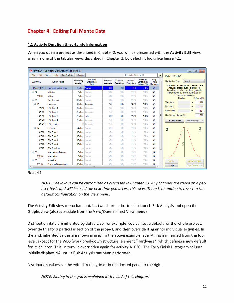
When you open a project as described in Chapter 2, you will be presented with the Activity Edit view,
which is one of the tabular views described in Chapter 3. By default it looks like figure 4.1.
Figure 4.1
NOTE: The layout can be customized as discussed in Chapter 13. Any changes are saved on a per-
user basis and will be used the next time you access this view. There is an option to revert to the
default configuration on the View menu.
The Activity Edit view menu bar contains two shortcut buttons to launch Risk Analysis and open the
Graphs view (also accessible from the View/Open named View menu).
Distribution data are inherited by default, so, for example, you can set a default for the whole project,
override this for a particular section of the project, and then override it again for individual activities. In
the grid, inherited values are shown in grey. In the above example, everything is inherited from the top
level, except for the WBS (work breakdown structure) element “Hardware”, which defines a new default
for its children. This, in turn, is overridden again for activity A1030. The Early Finish Histogram column
initially displays NA until a Risk Analysis has been performed.
Distribution values can be edited in the grid or in the docked panel to the right.
NOTE: Editing in the grid is explained at the end of this chapter.

12
4.2 Templates
There is an ability to define and apply templates to quickly enter data on activities with similar profiles.
Two templates are supplied with the product, but you can modify these and add your own. See Chapter
14 for further information on creating/editing templates.
NOTE: There must always be a template called “Default.” It is used as the default top level and is
initially inherited by all activities in a new project.
Templates can be assigned to one or more activities as follows:
To apply a template to a single WBS element/activity, simply right-click on the WBS/activity in the grid
and choose Apply Template from the context menu as shown in figure 4.2.
Figure 4.2
To apply a template to multiple WBS elements/Activities, select all the required rows using standard
keystrokes such as CTRL+Click, Shift+Click, or Click+drag. To select all rows, choose Select All from the
Edit menu or type CTRL+A.
NOTE: Activities in WBS Elements that are not expanded will not be selected by the above
selection operations and will not be directly updated by template application. However, if such
activities are set to inherit uncertainty information they may be affected by changes applied to
higher level WBS elements.
13
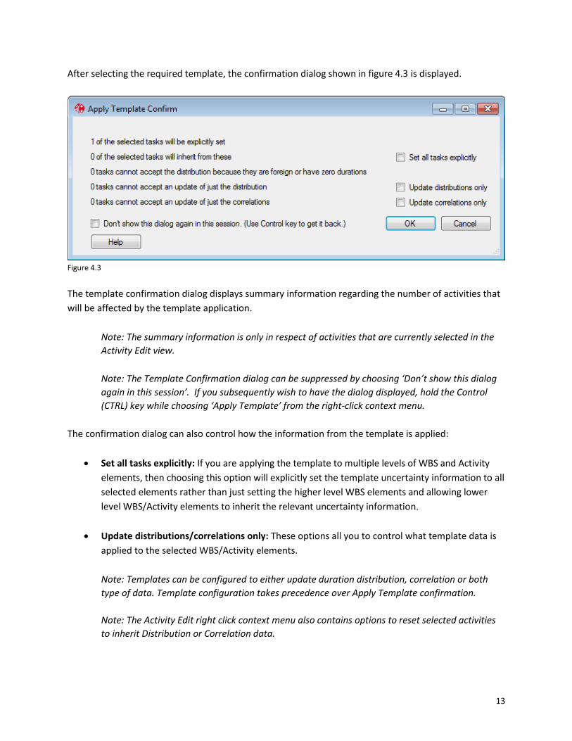
After selecting the required template, the confirmation dialog shown in figure 4.3 is displayed.
Figure 4.3
The template confirmation dialog displays summary information regarding the number of activities that
will be affected by the template application.
Note: The summary information is only in respect of activities that are currently selected in the
Activity Edit view.
Note: The Template Confirmation dialog can be suppressed by choosing ‘Don’t show this dialog
again in this session’. If you subsequently wish to have the dialog displayed, hold the Control
(CTRL) key while choosing ‘Apply Template’ from the right-click context menu.
The confirmation dialog can also control how the information from the template is applied:
Set all tasks explicitly: If you are applying the template to multiple levels of WBS and Activity
elements, then choosing this option will explicitly set the template uncertainty information to all
selected elements rather than just setting the higher level WBS elements and allowing lower
level WBS/Activity elements to inherit the relevant uncertainty information.
Update distributions/correlations only: These options all you to control what template data is
applied to the selected WBS/Activity elements.
Note: Templates can be configured to either update duration distribution, correlation or both
type of data. Template configuration takes precedence over Apply Template confirmation.
Note: The Activity Edit right click context menu also contains options to reset selected activities
to inherit Distribution or Correlation data.
14
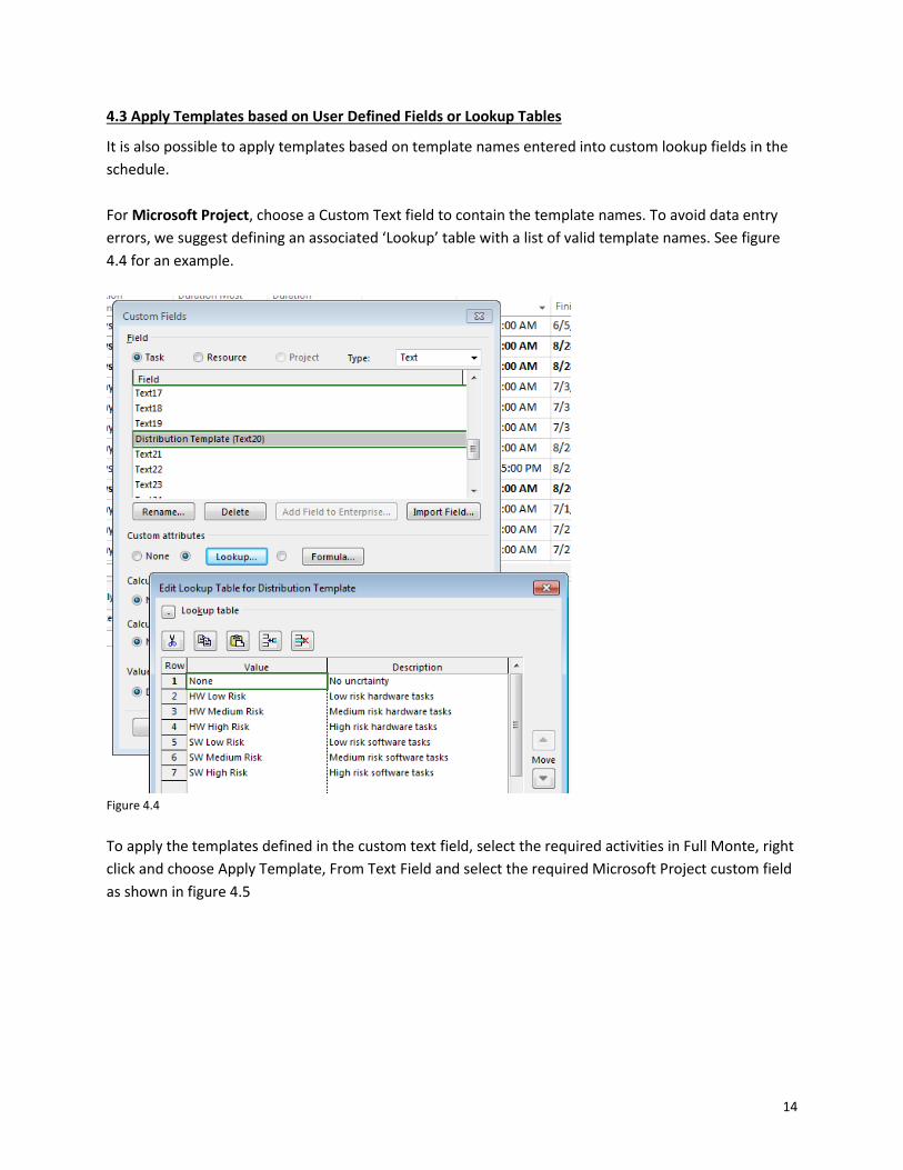
4.3 Apply Templates based on User Defined Fields or Lookup Tables
It is also possible to apply templates based on template names entered into custom lookup fields in the
schedule.
For Microsoft Project, choose a Custom Text field to contain the template names. To avoid data entry
errors, we suggest defining an associated ‘Lookup’ table with a list of valid template names. See figure
4.4 for an example.
Figure 4.4
To apply the templates defined in the custom text field, select the required activities in Full Monte, right
click and choose Apply Template, From Text Field and select the required Microsoft Project custom field
as shown in figure 4.5

15
Figure 4.5
For Primavera P6, define a custom Activity Code ‘Lookup Table’ as shown in figure 4.6
Figure 4.6
To apply the templates defined in the lookup table, select the required activities, right click, and choose
Apply Template, From Lookup Table and select the required Table as shown in figure 4.7

16
Figure 4.7
NOTE: The template name entered in the custom text/code field must match exactly with a
template name defined in Full Monte.
4.4 Manually Entering Uncertainty Information
If you do not want to use a template, you can enter the parameters individually. To assign a probability
distribution to the duration of this activity, first choose the general shape from the drop-down menu.
Five different shapes are available: beta, lognormal, normal, triangular, and uniform. To determine
which to choose for your application, see Appendix A, Probability Distributions.
Depending upon which probability distribution shape you choose, the controls will be enabled to allow
entry of either a 2- or 3-point estimate of the duration. The uniform, normal, and lognormal
distributions are each defined completely by two parameters, so Full Monte calculates the most likely
value for you. In either case, you can enter the information either as an absolute duration or a
percentage of the deterministic duration. (You are reminded of the current value of the deterministic
duration above the data entry fields.) Whichever entry method you use, Full Monte will prorate the
values when the activity is progressed or its duration has changed, so you will not have to update these
as the project progresses unless you want to.
You can also enter a confidence interval for the optimistic and pessimistic values you enter. By default it
is set to 100%, meaning you are 100% sure that the actual value will fall between the values entered.
NOTE: In the case of the triangular distribution, this is similar to what other systems call the
Trigen distribution. In Full Monte, this concept is extended to apply to all distribution types.
17
NOTE: 100% confidence cannot be strictly true for those distribution types that have infinitely
long tails, namely the normal and lognormal. In these cases, Full Monte interprets 100% as a 6-
standard-deviation range, or about 99.73%.
As you enter the data described above, the picture will change to indicate what the distribution function
actually looks like, with the optimistic, most likely, and pessimistic values marked, along with the
absolute limits if these are different.
NOTE: If the picture disappears, you have broken one of the rules defined in section 4.3.
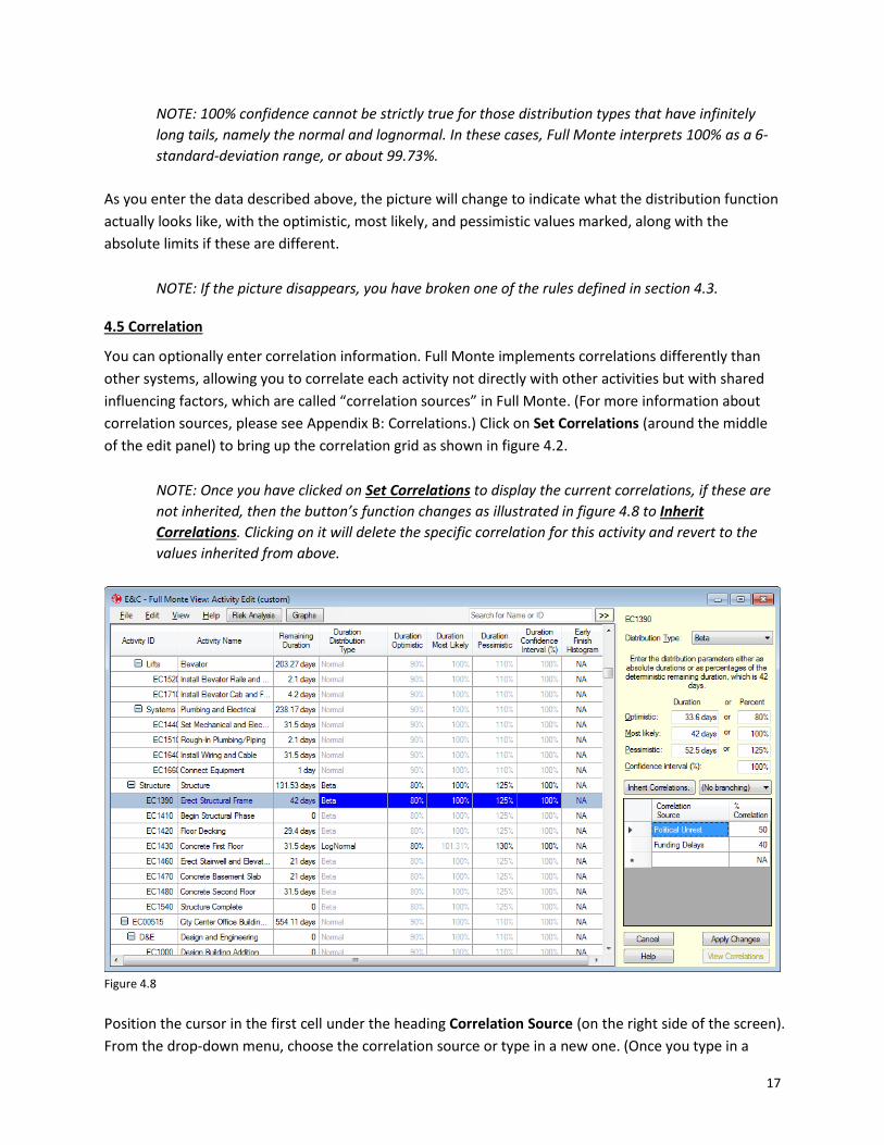
4.5 Correlation
You can optionally enter correlation information. Full Monte implements correlations differently than
other systems, allowing you to correlate each activity not directly with other activities but with shared
influencing factors, which are called “correlation sources” in Full Monte. (For more information about
correlation sources, please see Appendix B: Correlations.) Click on Set Correlations (around the middle
of the edit panel) to bring up the correlation grid as shown in figure 4.2.
NOTE: Once you have clicked on Set Correlations to display the current correlations, if these are
not inherited, then the button’s function changes as illustrated in figure 4.8 to Inherit
Correlations. Clicking on it will delete the specific correlation for this activity and revert to the
values inherited from above.
Figure 4.8
Position the cursor in the first cell under the heading Correlation Source (on the right side of the screen).
From the drop-down menu, choose the correlation source or type in a new one. (Once you type in a

18
correlation source, it will appear in the drop-down menu next time.) In the second column, enter a
percentage for the correlation coefficient. This should be between -100% and +100%, and the sum of
the squares of the values entered must not exceed 10,000 (i.e., if expressed as fractions rather than
percentages, the sum of squares cannot exceed 1).
Note that this correlation coefficient is between the duration of the current activity and the specified
correlation source. The correlation coefficient between any pair of activities correlated with this same
factor will be the product of the two entered correlation coefficients, interpreting them as fractions. For
example, if the two activities have coefficients of 50% and 70%, the correlation between the two activity
durations will be 35%.
NOTE: This also means that if you enter negative correlations for two activities, they will be
positively correlated with one another. If you want a negative correlation between two activities,
one should be negatively and one positively correlated with the source.
This novel way of specifying correlations allows Full Monte to properly model correlations between any
number of activities without the user having to resort to programming. (For more information on how
this works, see Appendix B: Correlations.) After you have applied the changes, you can see the implied
correlations with other activities by clicking View Correlations to display the grid illustrated in figure 4.9.
(This button is enabled only if there is at least one other activity correlated with the current activity.)
Figure 4.9
The grid shown in figure 4.9 lists all the activities correlated with the current activity, in descending
order of the theoretical correlation coefficient between each activity and the current activity. Clicking on
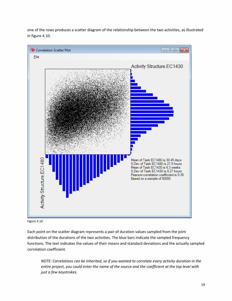
19
one of the rows produces a scatter diagram of the relationship between the two activities, as illustrated
in figure 4.10.
Figure 4.10
Each point on the scatter diagram represents a pair of duration values sampled from the joint
distribution of the durations of the two activities. The blue bars indicate the sampled frequency
functions. The text indicates the values of their means and standard deviations and the actually sampled
correlation coefficient.
NOTE: Correlations can be inherited, so if you wanted to correlate every activity duration in the
entire project, you could enter the name of the source and the coefficient at the top level with
just a few keystrokes.

20
4.6 Conditional Branching
The currently selected activity (EC1390) has multiple finish successors, so it is eligible for branching. Full
Monte supports two kinds of branching, conditional and probabilistic. Selecting a branching method
(conditional or probabilistic) in the drop-down menu will display the appropriate branching grid instead
of the distribution graphic. Figure 4.11 shows the conditional branching grid.
NOTE: For obvious reasons, branching cannot be inherited. Probabilistic branching is covered in
the next section.
Figure 4.11
For conditional branching, the choice of active successor depends on the finish date of the current
activity. Enter dates in all but one of the rows. Every date should be different. Using the above as an
example, the data is interpreted as follows: If activity EC1390 finishes on or before January 7th, then
choose activity EC1410. Otherwise, choose EC1420.
NOTE: You do not have to enter the dates in order, and the missing date can be anywhere. When
you click on Apply Changes, Full Monte will display them in order as shown in figure 4.5. If you
enter dates in every row, the latest date will be replaced with “NA.”
21
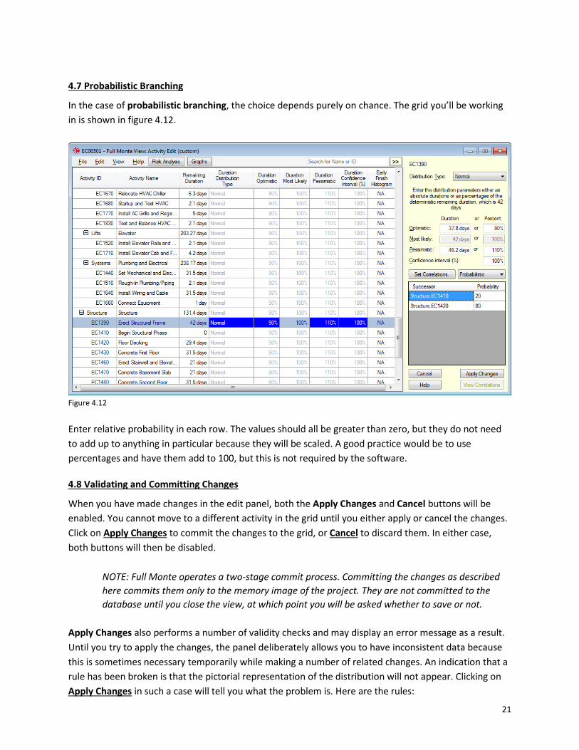
4.7 Probabilistic Branching
In the case of probabilistic branching, the choice depends purely on chance. The grid you’ll be working
in is shown in figure 4.12.
Figure 4.12
Enter relative probability in each row. The values should all be greater than zero, but they do not need
to add up to anything in particular because they will be scaled. A good practice would be to use
percentages and have them add to 100, but this is not required by the software.
4.8 Validating and Committing Changes
When you have made changes in the edit panel, both the Apply Changes and Cancel buttons will be
enabled. You cannot move to a different activity in the grid until you either apply or cancel the changes.
Click on Apply Changes to commit the changes to the grid, or Cancel to discard them. In either case,
both buttons will then be disabled.
NOTE: Full Monte operates a two-stage commit process. Committing the changes as described
here commits them only to the memory image of the project. They are not committed to the
database until you close the view, at which point you will be asked whether to save or not.
Apply Changes also performs a number of validity checks and may display an error message as a result.
Until you try to apply the changes, the panel deliberately allows you to have inconsistent data because
this is sometimes necessary temporarily while making a number of related changes. An indication that a
rule has been broken is that the pictorial representation of the distribution will not appear. Clicking on
Apply Changes in such a case will tell you what the problem is. Here are the rules:

22
1. The pessimistic value must be strictly greater than the optimistic value.
2. The most likely value (where applicable) must be between the two, inclusive.
3. Confidence must be between 50% and 100% inclusive.
4. The optimistic value must be no less than zero after adjusting for the confidence value.
5. For lognormal only, optimistic must be strictly greater than zero.
NOTE: The absolute minimum of a lognormal is always zero, but Full Monte interprets the
optimistic value so that about 1 in 750 samples fall between 0 and the optimistic value.
4.9 Editing in the Grid
Some users may prefer to edit the data in the grid. One advantage of this is that you can hide the edit
panel and thereby have more space to display columns of your choice. On the other hand, if you edit in
the panel, you do not need to show the editable columns in the grid. Other disadvantages are that you
cannot use templates nor edit correlations or branching.
Editable columns are shown in blue when the row is selected, as shown in figure 4.6. You can edit the
distribution type, the optimistic and pessimistic values, and where appropriate the most likely value.
You can use percentages or duration units.
NOTE: One other disadvantage of editing in the grid is that each change is validated as soon as
you leave the cell, so you may sometimes have to be careful in what order you make the changes.
For example, if you had a triangular distribution and wanted to change the optimistic value from
50 to 65 days and the most likely value from 60 to 75 days, you would have to make the second
change first to avoid breaking the rules even temporarily.

23
Chapter 5: Editing Full Monte Data for Resource Costs
Selecting the menu item Edit/Edit Resources takes you to a similar view for editing distributions on
resource cost rates.
NOTE: This menu item will be disabled if there are no cost rates associated with any resources
used by the project.
Figure 5.1
The view shows only those resources assigned to activities in this project. It works in a similar way to the
Activity Edit view.
For individual resources, you can enter data only if there is a cost rate defined. If there is only one rate
for the resource, you can enter the values in currency units. If there is more than one rate, that is if
there is cost escalation, all rates are assumed to move in unison and the distribution parameters must
be entered as percentages.
For higher levels in the resource hierarchy, data must be entered in percentage terms, and it is used as
defaults for the lower levels.
Correlations work in the same way as activity durations. Resource rates can be correlated with either
other resource rates or with activity durations or both.

24
NOTE: During the simulation, the cost of each activity is calculated using its resource usage and
the appropriate rate, having regard to any escalation.
When you have finished you can close the view, and you will be back in the Activity Edit view. You will
be prompted whether you want to save any changes made to the resource rate distributions.

25
Chapter 6: Editing Full Monte Data for Calendars
[This capability is available only in the P6 version.]
Selecting the menu item Edit/Edit Calendars takes you to a somewhat similar view for editing calendars.
It looks like the example shown in figure 6.1.
Figure 6.1
The view shows only those calendars assigned to activities in this project or to their resources. The way
calendars are modeled requires some explanation. There are four basic models:
1. Full days may be lost or not on a seasonal and random basis.
2. A randomly generated proportion of a day may be lost, this proportion being generated from a
lognormal distribution.
3. Full weeks may be lost or not on a seasonal and random basis.
4. A randomly generated proportion of a week may be lost, this proportion being generated from a
lognormal distribution.
The model is used in conjunction with an expected value for the particular week number. In the above
example, we expect to lose 20% of the working time between weeks 39 and 47 inclusive, and none at
the other times. During the simulation, Full Monte will interpolate the probability between specified
points, including wrapping around the year-end from the last week number to the first. (Any odd days in
week 53 are treated as part of week 52 for this purpose.)

26
NOTE: If your data is not seasonal, maybe because it has nothing to do with the weather, you
only need to add one row to the grid, and it does not matter what the week number is.
It is also possible to specify a correlation between consecutive days or weeks. This is meant to model the
extent to which one period affects the next and allows modeling of the fact that the weather is more
likely to be also bad on the day following an episode of bad weather. A default is provided of 50% for
daily models and 0% for weekly models, which is appropriate for some measures of the weather. (The
effect wears off rapidly with time. Raising 50% to the power of 7 — to get the weekly value — gives less
than 1%, which would not be material.)
NOTE: Correlations of more than 70% for daily models (8% for weekly models) are rarely
appropriate, especially when the probability of lost time is also high. With the discrete models
(full days or weeks lost) in particular, even moderate correlations when used in conjunction with
high probabilities of lost time for extended parts of the year can result in unintentionally long
periods with no working time, with consequent effects on project duration.
When you see the results (see Chapters 8 and 9), you will notice that this does not change the reported
duration, which is typically in working days, but it does change the elapsed duration. Two activities with
the same duration (in working days) may take different times (or elapsed durations) if they occur in
different periods. This is a much better way to model the weather than using correlations.
NOTE: Two activities that both depend on the weather in the same location are correlated only if
they happen at the same time, which, in theory at least, is not known in advance. Modeling the
connection with a correlation between the two durations is therefore not as realistic as modeling
the calendar as described above.

27
Chapter 7: Running Risk Analysis Simulation
This is done by clicking on the Risk Analysis button on any tabular view. (Doing it from any of the edit
views allows you to see the effect before committing the data changes.) This displays the dialog shown
in figure 7.1.
Figure 7.1
The edit controls are populated using the values last used for this project, or system defaults otherwise.
You can choose a number of options, as described below.
Number of Simulations: The larger this number, the better your results will be. Not only will your results
be more accurate, but the graphics will tend to be smoother and therefore more aesthetically pleasing.
The only downside to doing more simulations is the additional processing time. However, Full Monte is
fast, so you can afford to do more simulations than might be practical with slower products. We
recommend a minimum of 10,000.
Use Fixed Seed: Risk analysis uses what are called pseudorandom numbers. They are not really random
because if you know the algorithm you can predict the next value with perfect precision, but they
appear random and pass statistical tests for randomness. The pseudorandom number generator starts
with what is called a seed value, which by default is determined by the date and time. This means that if
you do the same risk analysis twice, you will get the same results only to the statistical accuracy of the
simulation. Unless you do a very large number of simulations, you will not always get exactly the same
results. If you want exact repeatability, check this box and the random number generator will be
initiated with the same seed value every time. We do not recommend this option because it creates a
false sense of repeatability. What you should do instead is increase the number of iterations until the
results are repeatable within the precision you require.
NOTE: The repeatability works only if no significant changes are made to the data. For example,
adding an activity or a correlation source will change the number of samples used in each
iteration so that the second and subsequent iterations will start with a different pseudorandom
number, negating the effect of using a fixed seed.
28
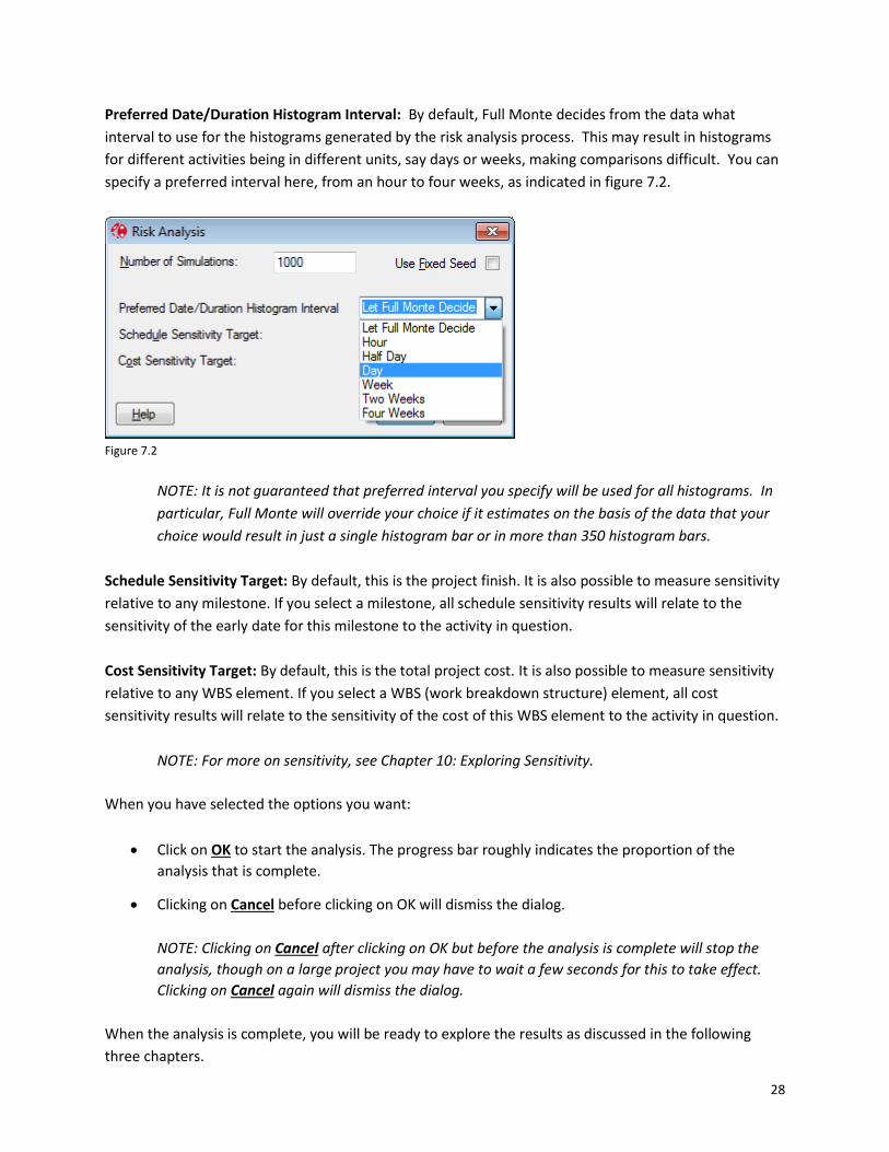
Preferred Date/Duration Histogram Interval: By default, Full Monte decides from the data what
interval to use for the histograms generated by the risk analysis process. This may result in histograms
for different activities being in different units, say days or weeks, making comparisons difficult. You can
specify a preferred interval here, from an hour to four weeks, as indicated in figure 7.2.
Figure 7.2
NOTE: It is not guaranteed that preferred interval you specify will be used for all histograms. In
particular, Full Monte will override your choice if it estimates on the basis of the data that your
choice would result in just a single histogram bar or in more than 350 histogram bars.
Schedule Sensitivity Target: By default, this is the project finish. It is also possible to measure sensitivity
relative to any milestone. If you select a milestone, all schedule sensitivity results will relate to the
sensitivity of the early date for this milestone to the activity in question.
Cost Sensitivity Target: By default, this is the total project cost. It is also possible to measure sensitivity
relative to any WBS element. If you select a WBS (work breakdown structure) element, all cost
sensitivity results will relate to the sensitivity of the cost of this WBS element to the activity in question.
NOTE: For more on sensitivity, see Chapter 10: Exploring Sensitivity.
When you have selected the options you want:
Click on OK to start the analysis. The progress bar roughly indicates the proportion of the
analysis that is complete.
Clicking on Cancel before clicking on OK will dismiss the dialog.
NOTE: Clicking on Cancel after clicking on OK but before the analysis is complete will stop the
analysis, though on a large project you may have to wait a few seconds for this to take effect.
Clicking on Cancel again will dismiss the dialog.
When the analysis is complete, you will be ready to explore the results as discussed in the following
three chapters.

29
Chapter 8: Named Tabular Views
8.1 Overview
Named views are read-only views that you can use to view various aspects of the project data, including
the results of Full Monte’s risk analysis, as well as the data used to generate it and a variety of source
scheduling system data (though by no means all). You can select the views by name from the
View/Open Named View menu available whenever a project is open.
Some named views are standard views that are hard-coded in the software and cannot be changed by
the user. Others are user-defined, in other words, created by the user.
NOTE: You can make changes to standard view and save the modified view under different
names using View/Save View Specification As, but you cannot overwrite the standard reports.
There are also a small number of features in the standard reports that cannot be added directly
by the user, so starting with a standard report is the only way to duplicate these. These are
described in section 8.3.
All views can be printed or copied to the clipboard.
8.2 Standard Views
When you select View/Open Named View, the standard reports are those listed above the line in the
drop-down menu shown in figure 8.1.

30
Figure 8.1
The top item, “(New),” is not so much a view as a starting point for developing your own new views. It
has just one column, the activity ID.
The other standard views are listed in alphabetical order and described below in the same order.
The view Graphs comprises a table of buttons from which you can view all the graphical results of risk
analysis. The report is illustrated in figure 8.2.
Note: The Graphs view can also be displayed by clicking the Graphs quick-launch button on the
Activity Edit view menu bar.
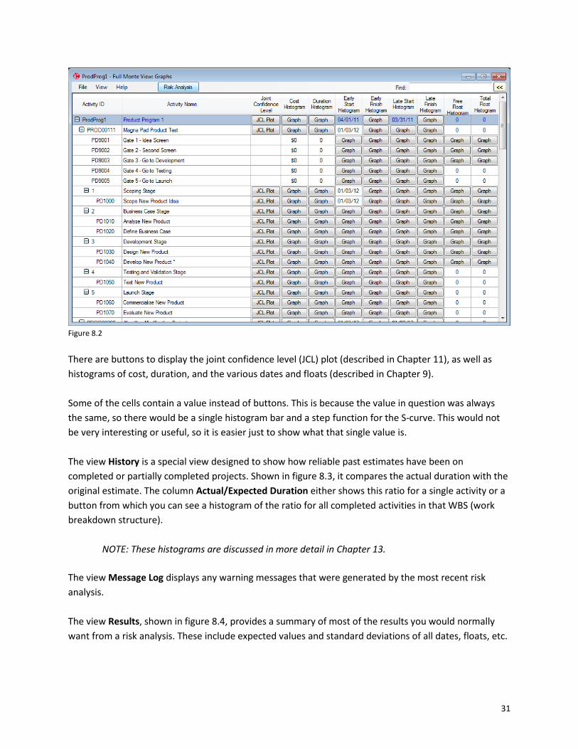
31
Figure 8.2
There are buttons to display the joint confidence level (JCL) plot (described in Chapter 11), as well as
histograms of cost, duration, and the various dates and floats (described in Chapter 9).
Some of the cells contain a value instead of buttons. This is because the value in question was always
the same, so there would be a single histogram bar and a step function for the S-curve. This would not
be very interesting or useful, so it is easier just to show what that single value is.
The view History is a special view designed to show how reliable past estimates have been on
completed or partially completed projects. Shown in figure 8.3, it compares the actual duration with the
original estimate. The column Actual/Expected Duration either shows this ratio for a single activity or a
button from which you can see a histogram of the ratio for all completed activities in that WBS (work
breakdown structure).
NOTE: These histograms are discussed in more detail in Chapter 13.
The view Message Log displays any warning messages that were generated by the most recent risk
analysis.
The view Results, shown in figure 8.4, provides a summary of most of the results you would normally
want from a risk analysis. These include expected values and standard deviations of all dates, floats, etc.

32
Figure 8.3
Figure 8.4
The three tornado charts are described in Chapter 10.

33
8.3 Special Features of Certain Standard Reports
1. The report Graphs contains a filter so that only rows with at least one Graph button will be
displayed.
2. All the Tornado charts contain a filter so that only rows with bars will be displayed.
3. All the Tornado charts respond to clicking on the bars to do a full sensitivity analysis as explained
in Chapter 10.
4. The Tornado reports contain special code to display the bars in two colors, split at the point of
the expected date of the sensitivity target. The user can control only the left-hand color.
There is no explicit user interface to include these behaviors in nonstandard views, but they will be
inherited by any user-defined reports based on them.

34
Chapter 9: Graphical Views
One final user interface element is the graphical view, which is accessed from the Graph buttons on any
histogram column included in a spreadsheet or the docked panel in tabular views. It looks like the
example in figure 9.1.
Figure 9.1.
The histogram bars show the frequency function measured against the left-hand scale, whereas the
S-curve shows the cumulative frequency function measured against the right-hand scale. You can
produce graphs at any level of the WBS (work breakdown structure) for:
Cost
Duration
Early Start
Early Finish
Late Start
35
Late Finish
Free Float
Total Float
The chevron buttons (<< and >>) allow you to move backward and forward through the list of activities.
The File menu allows you to:
Print the view
Show a print preview of the view
Copy the view to the clipboard
Close the view
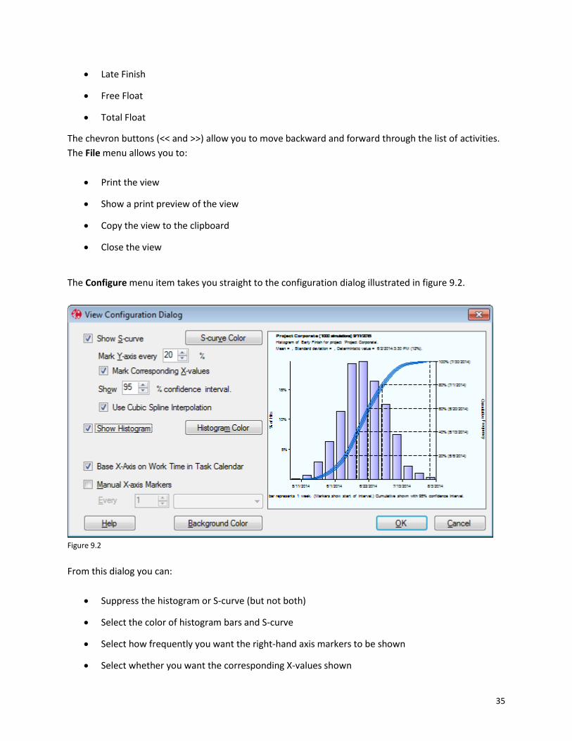
The Configure menu item takes you straight to the configuration dialog illustrated in figure 9.2.
Figure 9.2
From this dialog you can:
Suppress the histogram or S-curve (but not both)
Select the color of histogram bars and S-curve
Select how frequently you want the right-hand axis markers to be shown
Select whether you want the corresponding X-values shown

36
Select whether you want to show a confidence range around the S-curve (see below)
Select whether to use cubic spine or linear interpolation to form the S-curve (see below).
Select whether to base the X-axis on the task calendar (see below).
Define frequency of X-axis markers
Select the background color
Every time you make a change it is reflected in the preview on the dialog. In the example in figure 9.2,
the confidence interval for the S-curve has been set to 95%. This causes the S-curve to be replaced by an
envelope such that there is 95% confidence that the true cumulative probability lies within it.
NOTE: In this case, only 1,000 iterations have been done for illustrative purposes. The more
iterations you do, the narrower the envelope will be.
The S-curve is formed by interpolating between the cumulative values at the end of each histogram
interval. This can be done either linearly or using a technique called a cubic spline. This fits a cubic
function to each line segment such that where it meets its neighboring segments it has the same
gradient, avoiding sharp corners at these points. It generally produces a smoother and more realistic
curve, but in some cases (usually when too few iterations have been performed or when elapsed time is
used for the X-axis as dscussed below) it may be misleading.
The X-axis can be dispayed either using elapsed time (i.e. allowing space for non-work time such as
weekends) or usng the task calendar. Depending upon the histogram interval, using elapsed time may
result in gaps in the histogram (and horizontal lines in the S-curve) representing weekends or overnight
hours. Using the task calendar for the X-axis will not allocate any space for non-work time, eliminating
any spaces and making the S-curve smooth.
NOTE: The space allocated to each interval is actually proportional to the amount of work time
in it. This is normally either 0 or a constant value (e.g 0 on Sunday, 480 minutes on Monday) so
every period which is actually shown will be the same width. However, if for example the
calendar indicates a half-day on Saturday, then Saturdays will be allocated half the width of the
a normal weekday. To compensate, the height of the bar is doubled so that the area of the bar
represents the probabililty in that interval and the tops of the histogram bars are comparable to
the surrounding bars.
When you have finished making changes, you can apply them by clicking on OK or cancel them by
clicking on Cancel.
NOTE: Any changes you make will apply to the current session only, unless when you close the
view from which you invoked the graph you elect to save it. If you do save it, it will be stored with
the view specification.

37
Chapter 10: Exploring Sensitivity
10.1 Overview
Sensitivity analysis is sometimes seen as an alternative to Monte Carlo simulation as a way to deal with
uncertainty. Barbecana believes it is a valuable tool that not only augments simulation results, but needs
to be done in conjunction with the simulation.
To see why this is necessary, consider a sensitivity analysis done in isolation, sometimes called a “local
analysis.” The typical local analysis varies one variable at a time within certain limits and examines the
effects, all other things being equal.
The devil is in the detail of those last five words, because “all other things being equal” is generally
interpreted as meaning “all other variables taking their expected values.” To see how misleading this can
be, suppose you had 10 identical activities in parallel with a common successor, each of which could
take three to seven weeks with an expected value of four weeks. Looking at each of these activities one
at a time and assuming that the other nine took their expected value of four weeks, it would look as if
each of the activities had the potential to change the expected start of the successor by three weeks. In
fact, fixing one of them at three weeks and doing a full simulation would show that it has little effect,
because one or more of the other nine activities would be almost bound to take seven weeks to
complete. This “local” analysis ignores merge bias among all the other activities.
Full Monte therefore uses sophisticated statistical techniques to estimate the true sensitivity of each
activity during the simulation. Before going further, we should also note that it does sensitivity for both
cost and schedule, and that the user can choose the identity of the “sensitivity target” in each case. The
sensitivity target is the date or WBS (work breakdown structure) cost whose sensitivity to the input
variables one wishes to measure. The schedule sensitivity target defaults to the project finish but can be
set to any milestone. The cost sensitivity target defaults to the total project but can be set to any WBS
element.
NOTE: Only one of each type of target can be specified in any given risk analysis run. Doing them
all would require prodigious amounts of memory because the amount of data would be
proportional to the square of the number of activities.
The main sensitivity outputs are:
Sensitivity, Optimistic Finish of Target: This is an estimate of the expected early finish date of the
schedule sensitivity target if the current activity’s duration were to take its most optimistic value.
Sensitivity, Pessimistic Finish of Target: This is an estimate of the expected early finish date of the
schedule sensitivity target if the current activity’s duration were to take its most pessimistic value.

38
Sensitivity Index: This field gives an indication of how sensitive the early finish of the schedule
sensitivity target is to variation in the activity’s duration. It is computed as the percent critical multiplied
by the standard deviation of the duration and divided by the standard deviation of the early finish of the
sensitivity target.
NOTE: The field ‘Percent Critical (Sensitivity)’ is used in the Sensitivity calculation rather than the
regular ‘Percent Critical’ field. The field ‘Percent Critical (Sensitivity)’ differs in two ways from the
regular ‘Percent Critical’ field: it indicates whether the task is critical specifically to the sensitivity
target; and it reflects whether the duration of the task affects this target (so it does not count as
critical tasks which have the critical path passing through their starts or finishes but not through
their durations.
Sensitivity, Optimistic Cost of Target: This is an estimate of the expected cost of the cost sensitivity
target if the current activity’s duration were to take its optimistic value.
Sensitivity, Pessimistic Cost of Target: This is an estimate of the expected cost of the cost sensitivity
target if the current activity’s duration were to take its pessimistic value.
NOTE: The above two measures are produced for resource costs as well as for tasks.
NOTE: The cost sensitivity measures are more reliable than the schedule ones because costs
generally interact in simpler ways – i.e. they just add up. But note that schedule delays may
affect costs due to pushing a task into a time of higher unit cost due to escalation, while
conditional or probabilistic branching also make cost sensitivity non-trivial.
10.2 The Effect of Correlations on Schedule Sensitivity Calculations
In previous versions of Full Monte (and still used by most if not all other products) the methods used to
estimate the above measures of sensitivity (with the exception of the sensitivity index) were statistical
techniques based on a comparison of the inputs (the durations sampled for each activity) and outputs
(the early finish of the sensitivity target) as if the project network were a “black box.” They were
therefore vulnerable to being misled by correlations. If activity A and B are correlated and if activity A is
sometimes critical but activity B is not, then a correlation will nonetheless be observed between the
target date and the duration of task B, and this could result in a spurious indication that the target date
is sensitive to the duration of B.
The new technique used in Full Monte 2016 is based upon the relationship between the task duration
and the project finish date (or other specified target milestone date) only when the task is critical,
avoiding any errors due to correlation. It is still the case however that the only way to get completely
reliable estimates of the sensitivity to a particular task duration, while all other task durations are
uncertain, is to do two full risk analyses as described in section 10.4.
10.3 The Tornado Charts

39
The split tornado chart is illustrated in figure 10.1. The bars indicate the range of the expected finish
date based on possible variation in the duration of each of eight tasks. It was based on 10,000 iterations,
so we can be fairly sure that this is a definitive list. (It does not list activities for which the sensitivity is
not statistically significant.)
The chart is shown in descending order of the length of the bars, and the other measures of sensitivity
are in line. The dates upon which the bars are based are also shown in the columns on either side of the
bar chart. The bars are split by color at the expected finish date of the target.
NOTE: The bars are not necessarily symmetrical, and will often not be.
Clicking on a bar will do a full sensitivity analysis.
Figure 10.1
The cost tornado chart provides similar information for cost.
10.4 Full Sensitivity Analysis
Full sensitivity analysis for a particular task entails doing two risk analysis simulations, one with the
duration of the task set to its optimistic value and one with it set to its pessimistic value. In both cases,
all other tasks are allowed to vary randomly as defined by their distributions.
It is possible to do this full analysis for all the tasks shown in the view, or for individual tasks.
To do it for an individual task, click on the bar. You will get a dialog similar to the one shown in figure
10.2.

40
Figure 10.2
Clicking on Go sets off the full analysis which has three results:
1. A view showing the s-curves generated by the two simulations, as shown in figure 10.3, is
displayed. (This can be suppressed by unchecking the checkbox in the previous dialog.)
2. The dates and bars on the tornado view are updated to reflect the results of the full analysis.
3. The value of the “Schedule Sensitivity Bar Based on” field is changed to “Full Analysis”.
The view shown in figure 10.3 shows a pair of S-curves representing the cumulative frequency function
for the project finish on two alternative assumptions: that the duration of activity EC1290 takes its most
optimistic value and that it takes its most pessimistic value.
So now we have not just an estimate of the sensitivity of the expected value of the finish date, but of the
whole distribution! Furthermore, we can confirm that the sensitivity is about 3 months, and at the 50%
point this spans the dates 10/2 TO 1/7 as indicated on the tornado bar at the bottom of the view.
NOTE: The two S-curves are not always closely parallel as they are here. It is possible that a
target is considerably more sensitive to a task in one direction than the other.

41
Figure 10.2
When a full sensitivity analysis has been done for a particular task, this is indicated in the field “Schedule
Sensitivity based on” or “Cost Sensitivity based on” as shown for the second task in figure 10.3. The
colors of the corresponding bar are also slightly more vivid.

42
Figure 10.4
To perform a full analysis on all the tasks shown, right mouse on the bar column header and select “Do
Full Analysis for All Bars.” This invokes a dialog as shown in figure 10.5. This is similar to the previous
dialog but note that by default the checkbox is now unchecked.
Figure 10.5
NOTE: As noted above, cost sensitivity is generally simpler than schedule sensitivity.
Nevertheless, Full Monte supports the same functionality for costs to get a totally reliable
estimate from a full analysis. This will differ from the initial estimate only if branching or
escalation are involved.

43
Chapter 11: The Joint Confidence Level View
The joint confidence level (JCL) view is a scatter diagram showing the combined distribution of the early
finish date and the cost of the project or any activity or WBS (work breakdown structure) element. It can
be accessed by adding a column to the grid in the Project or Activity views or from a button on the
docked panel in the Project view. The view looks like figure 11.1.
Figure 11.1
Note that unlike other views, the data for this is not stored but is generated by doing a risk analysis
when required. For this reason, it takes some time to appear, especially for large projects and/or when
the project is not open. (The number of iterations performed is fixed at 5,000.) Because of this, you will
first see a dialog containing a progress bar and a Cancel button, as shown in figure 11.2.
NOTE: On very large projects that are not yet open, it may take 10 or 20 seconds for the progress
bar to appear. If you intend to open the project anyway, it is best to open it first and then access
this view from the grid.

44
Figure 11.2
If you proceed, you will see that the view is divided into four quadrants based on a target date and a
target cost. When the view first appears, these are both set to the 50th percentile, as in the example.
The green quadrant is where both cost and schedule are better than the target, while the red quadrant
is where they are both worse. The percentages in the corners give the percentage of observations in
each quadrant. (Because the view is initially centered on the 50th percentile, the percentages in
opposite quadrants are always equal. The more they differ from 25%, the more correlated the cost and
schedule.)
The view also shows three lines indicating points that have the same joint confidence level of 50%, 70%,
and 90%, respectively. (For example, any point on the 70% line has 70% of the points below and to the
left of it.)
The Configure menu item brings up the dialog shown in figure 11.3.
Figure 11.3
Here you can enter the real project targets, as well as a list of the constant JCL lines you want shown.
NOTE: Both targets must be within the ranges shown in the original plot.
This results in the report shown in figure 11.4. Note that there is roughly a 50% chance of meeting or
beating both the target date of 6/25 and the target cost of $7.2 million. (Note that there are many
combinations of date and cost target for which this is true, indicated by the 50% line.)

45
Figure 11.4.
The view can be printed or copied to the clipboard. The latter strips off the window border, as shown in
figure 11.5. (If you want the border, use Alt-PrtScrn.)
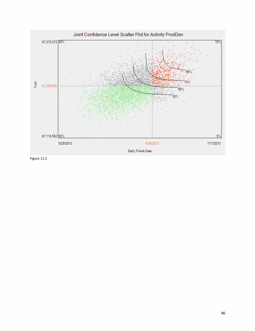
46
Figure 11.5

47
Chapter 12: The Actual/Expected View
The purpose of this view is to see how good your estimates have been in the past, so it is not very useful
until you have built up some history of completed projects. (You do not have to have performed risk
analysis on these projects though.) It can be done at any level in the WBS (work breakdown structure),
which contains at least two completed activities and plots the distribution of ratio of actual to expected
duration.
This data is accessed through the History view as illustrated in figure 12.1
Figure 12.1
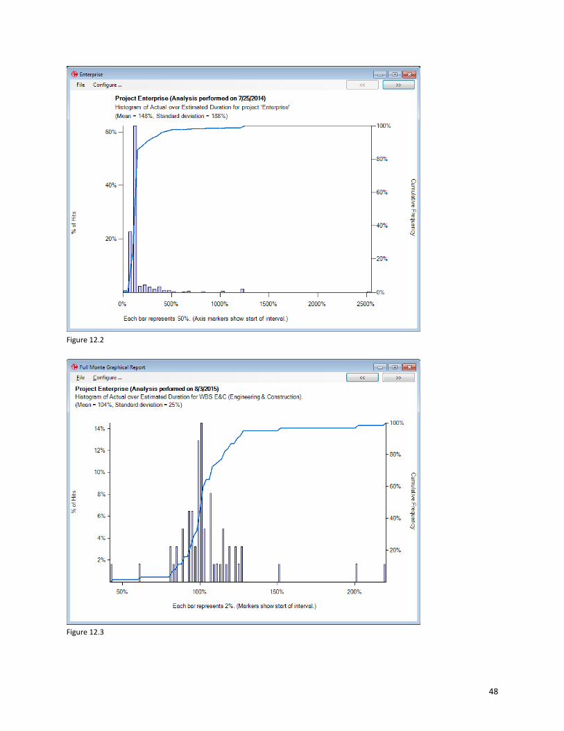
Clicking the Graph button on the top line produces the graph in figure 12.2. It shows the proportion of
activities throughout the entire organization/project/WBS element that completed on the ratio shown
on the X axis. This example is somewhat compromised by a single outlier, which took 250 times as long
as planned, but still you can see a familiar pattern. A little over 20% took between 50 and 100 percent,
and a little over 60% took between 100 and 150 percent of the expected value.
If you want to delve deeper, you can of course go down a level or two, though this reduces the sample
size. In figure 12.3, we have drilled down to one area of the organization, and you can see that while the
individual estimates vary widely, the overall average is remarkably good, at 104%.
48
Figure 12.2
Figure 12.3

49
Going back to the History report, we can also drill down in another way. Suppose we want to find that
2500% outlier. You will notice in figure 12.1 that in the graph column in some rows there is a percentage
instead of a button. This is true for all individual activities and for any WBS (work breakdown structure)
that contains only one completed activity. Using the right-click menu on the column header, select Find
in Column and type 2500. The result is shown in figure 12.4, from which we can see that the culprit is
activity A1470. It was a very short activity, so it may be of little consequence.
Figure 12.4
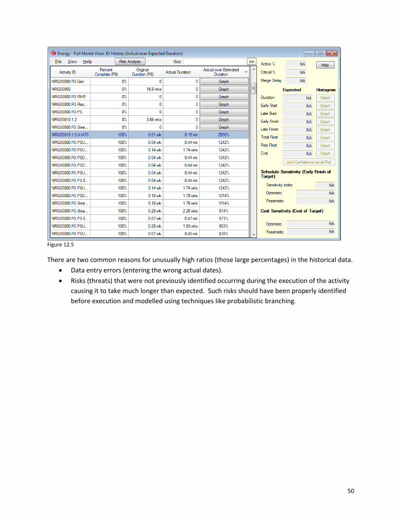
We were a little lucky there; we read off the value 2500% from the graph and searched for it, but it
might not have been exactly 2500%. An alternative would be to switch the hierarchy off and sort on the
graph column in descending order. All the graph buttons get sorted first and then the individual values
in descending order as shown in figure 12.5.
50
Figure 12.5
There are two common reasons for unusually high ratios (those large percentages) in the historical data.
Data entry errors (entering the wrong actual dates).
Risks (threats) that were not previously identified occurring during the execution of the activity
causing it to take much longer than expected. Such risks should have been properly identified
before execution and modelled using techniques like probabilistic branching.

51
Chapter 13: Customizing Views
13.1 Customization Options
The View menu allows you to:
1. Open a new named view
2. Save or Save As the current named view
3. Reset current view to its default settings (for unnamed views only)
4. Toggle whether to observe the hierarchy
5. Expand all nodes (disabled when hierarchy not shown)
6. Collapse all nodes (disabled when hierarchy not shown)
7. Sort the ID column interpreting numeric parts as integers (“Natural ID Sort,” on activity views
only.)
8. Undo the sort
9. Resize all columns to fit data
10. Select date format (only views that have the ability to display dates)
11. Set the default duration unit
Right-click on a column header to:
1. Find a value in the column
2. Sort on the column in ascending or descending order
3. Delete the column
4. Add a column before or after the column
5. Freeze the column (so it and all columns to its left stay put when you scroll)
6. Unfreeze the column (so it and all columns to its right scroll)
7. Resize the column to fit the largest item of data
8. Widen the column if necessary to make the total width of the grid fill the space
9. Edit the bar-chart definition (for bar-chart columns only)
Other customizations include:
1. Resizing columns by dragging or double-clicking the right edge of the header cell
2. Moving columns by dragging the header cell
52
3. Sorting on a column by clicking on the header cell (first time on a column ascending, second
time descending)
4. Show or hide the information panel by clicking on the chevron button (<< or >>)
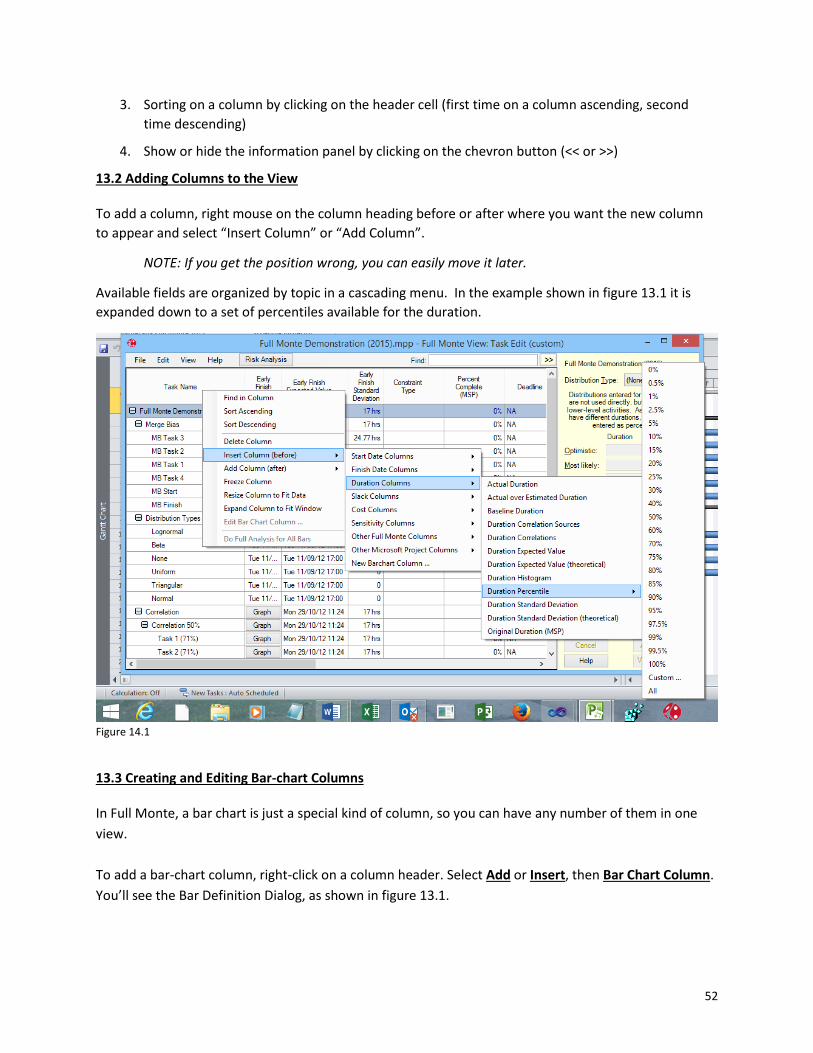
13.2 Adding Columns to the View
To add a column, right mouse on the column heading before or after where you want the new column
to appear and select “Insert Column” or “Add Column”.
NOTE: If you get the position wrong, you can easily move it later.
Available fields are organized by topic in a cascading menu. In the example shown in figure 13.1 it is
expanded down to a set of percentiles available for the duration.
Figure 14.1
13.3 Creating and Editing Bar-chart Columns
In Full Monte, a bar chart is just a special kind of column, so you can have any number of them in one
view.
To add a bar-chart column, right-click on a column header. Select Add or Insert, then Bar Chart Column.
You’ll see the Bar Definition Dialog, as shown in figure 13.1.

53
Figure 13.1
The drop-down menu at the top of the dialog allows you to select the type of data to display. This must
be date, duration, or cost/numeric. Since you cannot mix these types, once you have defined a bar this
control is disabled.
In the grid, you can define any number of bars and/or milestone symbols. Bars extend from Bar Start to
Bar Finish. For a milestone symbol, leave out one of the values. For example, for a finish milestone, leave
out the Bar Start or select “(None).” For a start milestone, leave out the Bar Finish. Select fields by
selecting from the drop-down list that appears when you click on the cell or by right-clicking on the cell.
For cost/numeric bars, there is an additional option for the Bar Start or Finish to be zero, enabling you to
display bars with lengths that represent the value of a particular cost or numeric field.
Enter a line for each bar or symbol you want to define. The grid will scroll if necessary. Figure 13.2 shows
a completed Bar Definition Dialog. Here is an explanation of the data:
Bar Start: The variable representing the start of the bar. Note that on the third row, this is set to
“(None),” making it a finish milestone symbol.
Bar Finish: The variable representing the start of the bar. Note that on the second row, this is set to
“(None),” making it a start milestone symbol.
Line Number: The line number allows you to separate bars and symbols vertically.

54
NOTE: Bars are displayed in the order in which they are defined. Unless you know that they won’t
overlap, you probably want to either separate them vertically or make the latter bar thinner. You
can alter the display order using the up and down arrow buttons to the right of the grid.
Lines are numbered from top to bottom within the cell, and the numbers do not have to be consecutive
(Full Monte closes up any gaps). If you don’t enter a line number, it will be taken as 1.
NOTE: A bar or symbol will not appear if the dates are not populated. For example, if you want
to draw a bar from actual start to early start to show progress, it will appear only if the activity
has been progressed.
Figure 13.2
Color: Clicking on the next cell invokes a color choice dialog where you choose the color of the bar or
symbol.
Bar Height: It is very important to enter the bar height, because a zero-height bar will simply not display.
The bar height is expressed as a percentage of the total cell height. The heights are scaled if necessary,
so that their total does not exceed 90%.
NOTE: A bar height of 1, as on the first row in the example, will produce a thin line. If you want
to temporarily suppress a bar without losing its definition, set its bar height at 0.

55
Full Monte applies a height to each line based on the bar or symbol with the greatest height in that line,
and then it applies the rule to the line heights. This avoids double counting bars and symbols on the
same line.
Show Zero-Length Bars: This check box specifies whether to print a symbol when the start and finish of
the bar are identical so that the bar would otherwise not display. (It has no effect if one end of tte bar s
“(None)” and it does not display if the end of the bar is to the left of the start of the bar.)
Sort Order: The final column in the grid controls the sort order.
NOTE: It does not actually sort the report; it defines what will happen when you sort on this
particular column by clicking on its header.
Click on the cell and select the sort order from the drop-down menu at the top of the screen or by right-
clicking on the cell. You can sort on only one bar or symbol, so when you select one the others will
revert to (None). For bars, you can choose to sort on either end or on the length of the bar. For symbols,
you can sort only on the value that it is based on.
There is also a text box and there are also fIve checkboxes controlling the display of the bar-chart
column as a whole:
Column Header Text allows you to annotate the column.
Don’t Display Rows with no Bars will suppress any rows for which there are no bars. The main reason
for there to be no bars is that the dates at both ends of the bar are the same for this particular activity.
For example, in the tornado report the bars appear only for activities that can affect the project finish
date, which is often a very small subset.
NOTE: If there is more than one bar-chart column, checking the checkbox Unless there are Bars
in Other Bar Columns on all of them will not suppress the row unless there are no bars in any
column.
Extend Grid Lines Downward extends the lines from the lowest level of the date grid in the header row
downward over the data rows.
Show Nonwork Time causes nonwork time to be displayed as a gray stripe underneath the bars. It
displays these only to the granularity of the lowest-level grid markings, so weekends will not show up
unless the grid is marked in days or less.
NOTE: This and the following checkbox are disabled if the data type is not Date.

56
Split Bars for Nonwork Time causes nonwork time to be indicated by a break in the bars. This break will
be either white or gray depending on the setting of the previous option. It splits the bars only to the
granularity of the lowest-level grid markings, so weekends will not show up unless the grid is marked in
days or less.
When you are done, click on OK. A column will appear before or after the place you right-clicked,
looking similar to the bar chart shown in figure 13.3. In this example, the Extend Grid Lines Downward
checkbox was checked.
Figure 13.3
NOTE: Right-clicking on the bar-chart header and selecting Edit Bar Chart Column will bring up
the dialog shown in 13.2 again so you can make changes.
13.4 Saving Your Customizations
For standard named views (those that appear above the line on the Open Named View drop-down
menus, you can save your changes to a new view name, using View/Save View Specification As.
For nonstandard named views you can do as above, or you can overwrite the original using View/Save
View Specification.

57
NOTE: With either type of named view, if you make changes during a session, you will be
prompted as to whether you want to save them when you close the view.
For unnamed views (that is the Project View and the three views used to edit activities, resources, and
calendars), any changes are automatically saved on a per-user basis and used the next time you access
that view. (As noted above, there is an option to revert to the original default.)
58
Chapter 14: Managing Percentiles, Templates, and Views
Percentiles, Templates, and Views are stored in the database [P6] or on the local disc [Microsoft Project],
and Full Monte provides simple dialogs to manage them.
Management dialogs are accessed from the Edit menu.
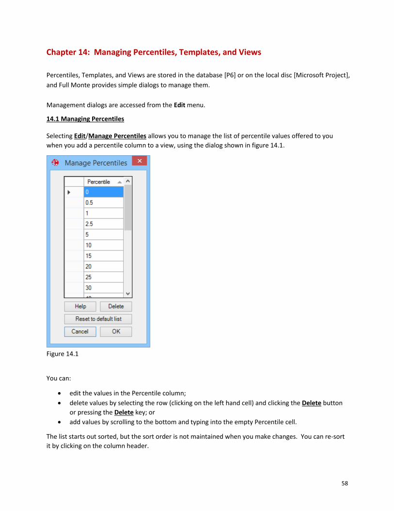
14.1 Managing Percentiles
Selecting Edit/Manage Percentiles allows you to manage the list of percentile values offered to you
when you add a percentile column to a view, using the dialog shown in figure 14.1.
Figure 14.1
You can:
edit the values in the Percentile column;
delete values by selecting the row (clicking on the left hand cell) and clicking the Delete button
or pressing the Delete key; or
add values by scrolling to the bottom and typing into the empty Percentile cell.
The list starts out sorted, but the sort order is not maintained when you make changes. You can re-sort
it by clicking on the column header.

59
NOTE: The dialog does not prevent you from temporarily creating duplicate values, but these
will be removed when you click OK.
There is also a button to revert to the system default as supplied by Barbecana when installed.
When you are done, click OK. Full Monte will sort the values, remove duplicates and update the list.
NOTE: These are personal preferences. They are stored on the local machine in the MSP version
and by user in the P6 version.
14.2 Managing Templates
The Manage Templates dialog is shown in figure 14.2. This allows you to add, modify, and delete
templates. You cannot delete the template called “Default,” but you can redefine it.
NOTE: Full Monte remembers each user’s active template between sessions. Since in the P6
version templates are global, it is possible that one user’s active template can get deleted by
another user. If this happens, Full Monte defaults to the one called “Default.”
To modify an existing template, select it from the drop-down menu and change the data as required.
Click Save to save the changes or Cancel to cancel them.
The actual data that you can specify are the distribution type and parameters and correlations. These
work as discussed in Chapter 4. (For obvious reasons, you cannot create template data for branching.)
To add a new template, click on New (which gives you a copy of the currently selected template), give it
a name, and change the data as required. Click on Save to save the changes or Cancel to cancel them.
To delete a template, select it from the drop-down menu and click on Delete.
Figure 14.2
60
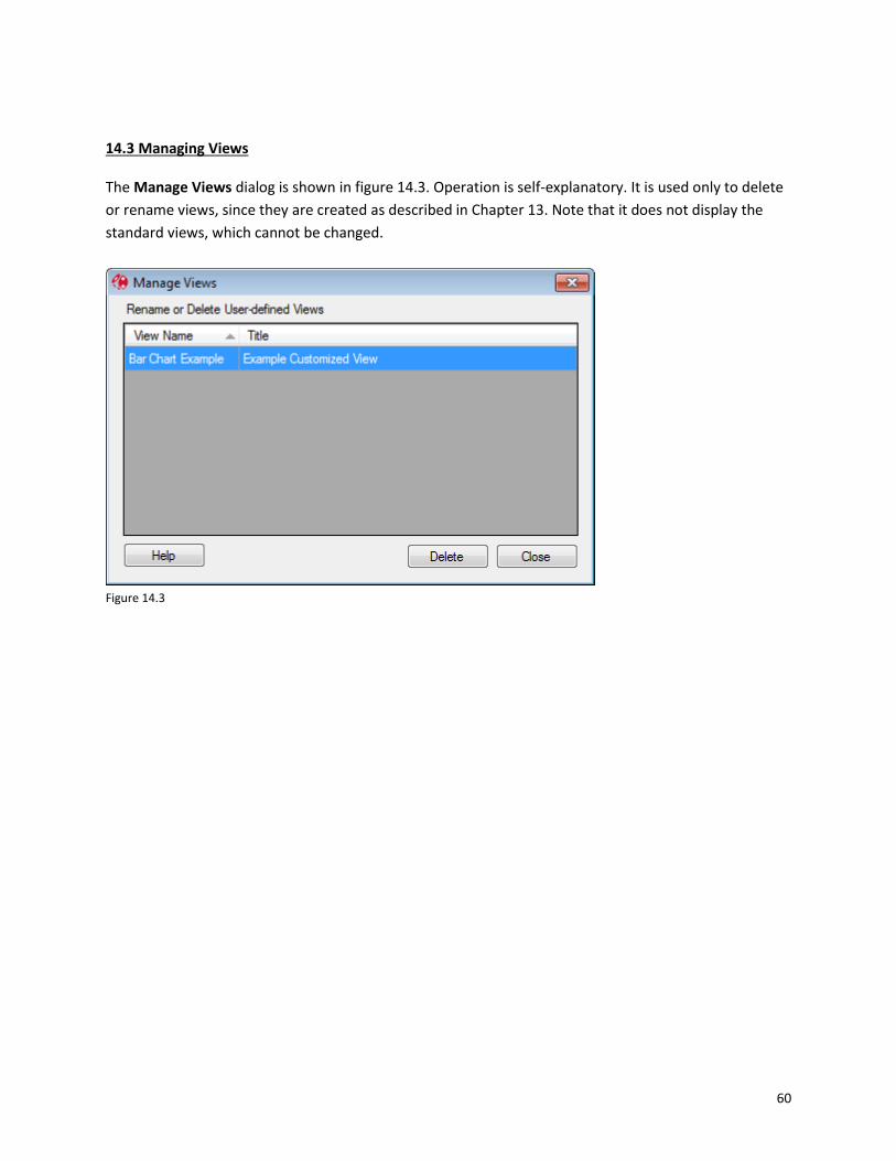
14.3 Managing Views
The Manage Views dialog is shown in figure 14.3. Operation is self-explanatory. It is used only to delete
or rename views, since they are created as described in Chapter 13. Note that it does not display the
standard views, which cannot be changed.
Figure 14.3

61
Appendix A: Probability Distributions
A probability distribution for a random variable is a function defining the probability of that variable
having a particular value. (The distributions used in Full Monte are continuous, which means that the
probability of any particular value is infinitesimal. It would be more accurate to talk about “the
probability density at a particular value.” Since Full Monte actually works in whole minutes and
approximates the continuous distribution by a discrete one, we can set aside this nicety for now.)
Both the inputs to Full Monte (activity durations, etc.) and the resulting outputs (dates, floats, and costs)
are probability distributions. The ones that come out are empirical, which means that we don’t have a
formula for the function; we have only an estimate based on simulation. Here we are concerned with
the probability distributions we input for activity durations and cost rates, where we do have such a
formula.
Full Monte supports five families of probability distributions. Here we discuss what they are, how you
choose among them, how the parameters are interpreted, and how Full Monte samples from them.
Uniform distribution
The simplest distribution type is the uniform distribution, in which any value in a specified range is
equally likely. Unfortunately, it is also the least useful because it is unlikely to be realistic in practice. (If
you think that an activity will take between four and six weeks, the actual value is probably more likely
to be toward the center of the range rather than near the outer edges.)
Sampling is merely a matter of translating a pseudorandom number (which emulates a true random
variable distributed uniformly between 0 and 1) to the specified range. That range is specified by the
user on the Full Monte Edit dialog. Since the distribution is symmetrical, there is no need to input a
middle value. (The dialog calculates and displays what it calls the most likely value, though in this
particular case it is actually the mean value. By definition, no value is more likely than any other.) An
example of the uniform distribution as generated by Full Monte is illustrated in figure A.1.
62
Figure A.1
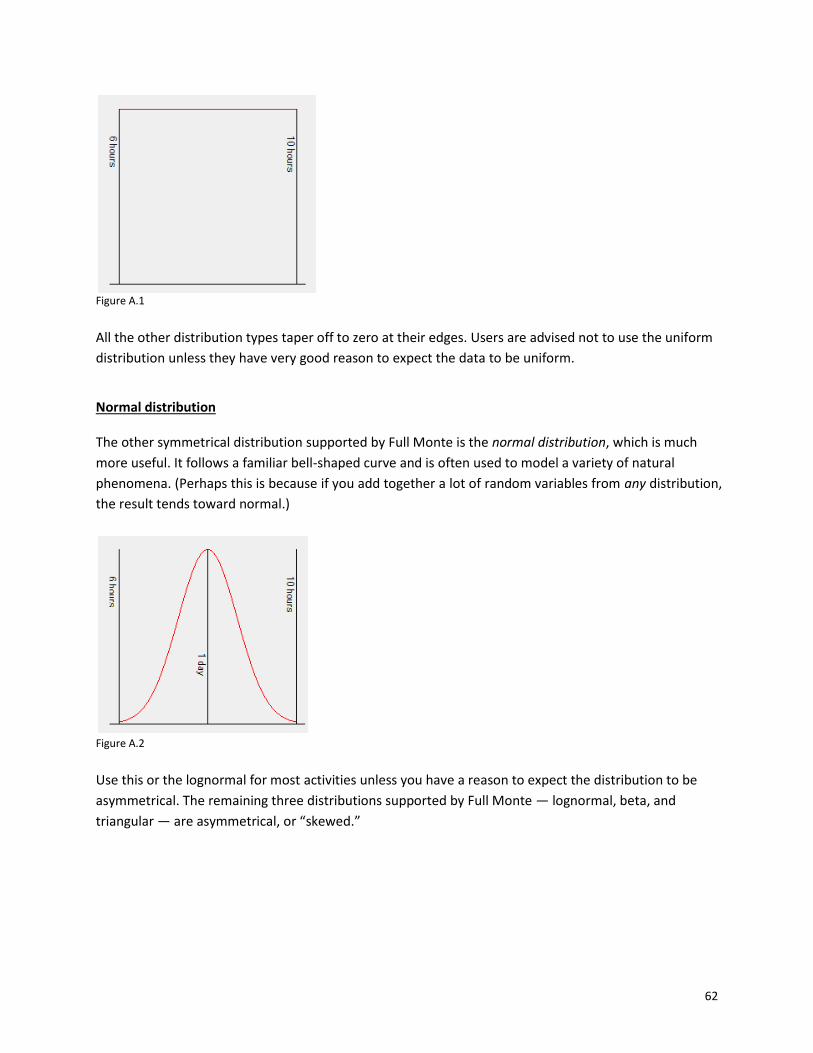
All the other distribution types taper off to zero at their edges. Users are advised not to use the uniform
distribution unless they have very good reason to expect the data to be uniform.
Normal distribution
The other symmetrical distribution supported by Full Monte is the normal distribution, which is much
more useful. It follows a familiar bell-shaped curve and is often used to model a variety of natural
phenomena. (Perhaps this is because if you add together a lot of random variables from any distribution,
the result tends toward normal.)
Figure A.2
Use this or the lognormal for most activities unless you have a reason to expect the distribution to be
asymmetrical. The remaining three distributions supported by Full Monte — lognormal, beta, and
triangular — are asymmetrical, or “skewed.”

63
Lognormal distribution
The lognormal distribution is skewed in a very special way. It is the distribution of a variable whose
logarithm is distributed normally, which means it is defined by just two parameters. Therefore, you
cannot specify the most likely value, so you cannot determine the skew independently of the optimistic
and pessimistic values.
It is always skewed to the right, or “positively.” The tail on the right is longer than the tail on the left. In
fact, while it has an infinite tail to the right, its absolute minimum is always zero since the log of minus
infinity is zero. When the optimistic and pessimistic values are close together the lognormal differs little
from the normal, but as the ratio between the two increases the skew becomes greater.
The lognormal also occurs often in nature for values that can vary by orders of magnitude. (Which is why
when you look at a list of populations of cities of all sizes, you find that about 30% of them have 1 as
their first digit.) Use the lognormal for situations where the duration is highly uncertain, such as basic
research projects, where the pessimistic estimate may exceed the optimistic by an order of magnitude
or more. There is even some empirical evidence from Dan Trietsch of the American University of
Armenia that the lognormal distribution should be used in all cases. (See
mba.tuck.dartmouth.edu/pss/Notes/LognormalParkinson.pdf.)
Two examples of the lognormal distribution as generated by Full Monte are illustrated in figure A.3. The
first is less extreme, with the minimum value being 60% of the maximum, making it almost symmetrical,
while the second has a minimum, which is only 10% of the maximum.
Figure A.3
The final two supported distributions are determined by three parameters and thus give the user
complete control over the amount and direction of the skew.

64
Beta distribution
A true beta distribution is specified by no less than four parameters, which give rise to an astonishing
variety of shapes, many of which would not be expected or useful, such as continuously increasing or
decreasing or even a U-shape with the lowest point in the middle. (See the Wikipedia entry referenced
in the Bibliography. It also includes the uniform distribution as a special case, but in Full Monte we treat
this separately.)
Full Monte therefore restricts the choice to a well-behaved subset that rises monotonically from zero at
its most optimistic point until it reaches its peak, and then declines monotonically to zero at its most
pessimistic point. In fact, the particular subset used by Full Monte when defined to be symmetrical looks
almost identical to a similarly defined normal distribution and has an almost identical standard deviation.
The standard deviation decreases, however, as the skew increases. Two examples of the beta
distribution — one symmetrical and one skewed to the right — are illustrated in figure A.4.
NOTE: The particular subset is intended to approximate to the distribution used in PERT, but this
is somewhat ambiguous. The formula suggested for the mean — (a + 4b + c) / 6 — implies one
subset, while that suggested for the standard deviation — (b – a) / 6 — implies another. Full
Monte has chosen the latter, which means that in the symmetrical case the standard deviation is
actually equal to that of the normal. (It decreases with increasing skew to about 1/9th of the
range.) This also means that the mean is actually given by (a + 6b + c) / 8.
Figure A.4
Use this distribution when you want something similar to a normal distribution but want to control the
skew.
Triangular distribution
Finally, the triangular distribution has long been used for schedule risk analysis. It does not appear much
naturally, but it is simple, and because it puts more emphasis on values close to the limits, it is perhaps
more in tune with users’ expectations. As its name implies, it is simply a triangle with the base defined
by the optimistic and pessimistic estimates, and the apex defined by the most likely value. It is very easy

65
to sample and to understand, but like the uniform distribution, it is unlikely to reflect the real situation.
Because its tails are not thin, it has a larger standard deviation than similarly defined distributions of all
the other types except uniform. Two example of the triangular distribution — one symmetrical and one
skewed extremely to the right with the same parameters as the beta above — are illustrated in figure
A.5.
Figure A.5

66
Appendix B: Correlation
Correlation is the name given to the phenomenon of interdependence between random variables, such
that the frequency function for one of them depends on the actual values of the others. For two
variables, it is often illustrated visually by a scatter diagram. To fully describe the correlation between
two or more variables mathematically, one must define their multivariate distribution function, which is
a multidimensional extension of the frequency function defining the probability of each possible
combination of values of the variables. For most purposes, however, and certainly for input to Full
Monte and other schedule risk analysis software, we summarize this using the concept of correlation
coefficients.
A correlation coefficient measures the degree of interdependence between two random variables in
terms of a number between -1 and 1. The details are beyond the scope of this guide and there are
actually two different correlation coefficient definitions. The interested reader is referred to the URLs
listed in the bibliography. Suffice it to say that a coefficient of zero means that the variables are
independent, while a coefficient of + or - 1 means that they are perfectly (positively or negatively)
correlated, i.e., the value of one variable exactly determines the value of the other.
It is worth noting, since it surprises some people, that perfect correlation can exist even between
variables with different distributions, as illustrated in the scatter diagram in figure B.1. (Actually, the
Pearson or linear correlation coefficient displayed is not quite 1 but the Spearman correlation coefficient
is exactly 1. But more to the point, any particular value of one of the variables precisely determines the
value of the other.)

67
Figure B.1 100% correlation between a uniform and a lognormal distribution
It is also worth noting that the correlation coefficient measures linear, or at least monotonic
relationships. A Wikipedia URL referenced in the Bibliography shows how various convoluted
relationships can exist between variables that have zero correlation coefficients. The correlations in Full
Monte can, however, be relied upon not to exhibit such odd relationships and a typical correlation
between two activity durations is illustrated in figure B2.
Figure B.2 Approximately 80% correlation between a uniform and a lognormal distribution

68
So, correlation coefficients provide a shorthand way of defining the joint distribution of two variables,
which more generally would require us to define the joint distribution in detail. But even using
correlation coefficients, specifying the relationship between three or more variables can be a daunting
task. To properly describe the correlations between the three variables, one needs to define the
correlations between each of the three possible pairings. And it gets much worse: If there are four
variables involved there are six possible pairings, and for five there are 10.
Full Monte handles correlations between the durations of activities differently than other systems.
Some allow the user to specify the correlation between the durations of any two activities, but this does
not fully define the relationship between a larger set of activities. Suppose that five activities (A through
E) are correlated in a symmetrical fashion, i.e., the correlations between any pair are the same. There
are 10 possible pairings, but in simple systems only five places (one on each activity) to enter a
correlation with another activity. What happens is that you pick an activity arbitrarily (say A) and
correlate the others with it. Let’s say you put in 50% as the correlation coefficient. The result is that B, C,
D, and E are correlated with A at 50%, but are correlated with each other only 25% (50% turned into a
fraction and then squared). So the symmetry is not accurately modeled.
Some systems ignore this problem, which means they do not properly handle correlations involving
more than two activities, while others require the user to write code to set up the data in a strictly
upper triangular matrix. Other systems support “drivers,” an idea discussed in the next section.
Full Monte takes a different approach, recognizing that the usual reason for a correlation between the
durations of different activities is that they all depend upon some outside factor, such as their location.
We make this explicit, so that however many activities there are, each of them just needs one scalar
quantity to define its correlation with a particular factor, and hence with all other activities similarly
defined. So all the user has to enter for each activity is the causal factor (which can be given any
arbitrary name like “On Site”) and the correlation coefficient. Any number of such factors can be
included, and once specified for one activity they appear on the drop-down list for the others.
Of course if the situation really is asymmetrical, so that activities B and C really do depend on activity A
(and are therefore more correlated with A than with each other), then all you have to do is define a
factor (say activity A) and make A correlated with that with a coefficient of 100%.
Note that in the symmetrical situation described above, one should enter the square root of the
correlation you want between each pair of activities. So instead of putting in 50%, one would put in 70%
(the square root of .5 is actually about 0.707).
Correlation Sources vs. Drivers
Drivers are a recent development that seems superficially similar to the Correlation Source concept
described above, but the concepts are similar only in that they both allow the user to specify one or

69
more outside factors to influence a set of activity durations, but the way in which this influence is
specified is very different. In the driver concept, the value of each driver is drawn from a distribution
roughly centered on 1, and they are interpreted multiplicatively. For example, if an activity is affected by
two drivers, these might be represented by two triangular distributions with parameters:
0 .7, 1.0, 1.2, and
0.9, 1.0, 1.4.
On a particular iteration, we might sample 1.04 and .98, so the value sampled for the activity is
multiplied by 1.04 times .98, or 1.0192.
While there is appealing logic to this seemingly simple idea, there are a number of problems for the
unwary that can be overcome only with the most sophisticated analysis:
1. First, it means that the distribution specified for the activity itself is not actually the distribution
you get. Even in the above relatively simple scenario, most statisticians would be hard put to tell
you what the final distribution is. In fact, one cannot readily calculate even the expected value
or standard deviation. (They are about 1.06 and .15, respectively, by the way.)
2. Second, one cannot readily know what the correlation coefficient between two activity
durations actually is.
3. Third, you cannot easily specify that two activities be affected by the same driver but to
different degrees. (This is possible, but involves complicated calculations to get the right input
data.)
4. Fourth, it is just additional data entry. It has been suggested that it can actually require less data
entry, on the basis that all the uncertainty in activity durations is attributable to drivers. Or that
any remaining uncertainty can itself be attributed to a special driver. But this is a fallacy. Using
the same driver to represent the uncertainty on two activities would make them unintentionally
correlated.
The net result is a system, which while it may have value in special circumstances, is likely to mean
either much more work or unrealistic results.
By contrast, correlation sources require no extra data other than the name of the source and a
percentage. They enable the user to easily specify correlations between any number of activities and
any number of sources and to simply calculate the correlation implied between any pair of activity
durations. (Full Monte even provides a visual aid in the form of a scatter diagram.) Furthermore, the

70
distribution the user specifies for the activity duration is unaffected by the correlation sources. One
incidental advantage of this is that it is easy to assess the effect of correlations.

71
Appendix C: Branching
Branching is a feature that enables Full Monte to choose at run time, i.e. on each iteration of the
simulation, which of a number of alternative paths from an activity is active. Full Monte supports two
types of branching: conditional and probabilistic.
In conditional branching, the user associates a date with each successor, such that the successor will be
active if it can start before that date, and no other successor with an earlier associated date can.
In probabilistic branching, the user specifies a set of relative probabilities for the different successors,
and the active successor will be chosen randomly based on these probabilities.
NOTE: Either type of branching can be applied to the finish-to-start successors of any activity
that has two or more of these. It does not apply to other types of relationships, and you cannot
combine the two different types of branching on successors to the same activity.
It is important to understand that branching applies to a path rather than an activity, which can lead to
several rather confusing scenarios.
For example, if successor activity C is not on the selected active path out of activity A, it could still itself
be active if it has another predecessor B that is active. The general rule is that:
NOTE: An activity is active if it is a start activity or if it has at least one active predecessor
relationship from an active predecessor.
Having stated the rules, it is probably best to avoid such confusing situations by using branching
judiciously. We suggest that the use of branching be limited to situations where no successor activity
has any other predecessors.
Branching and progress
If any of the successors have been progressed, Full Monte assumes that the branch has been
determined and will not apply the normal rules. In fact, it is quite possible (though illogical) that more
than one of the successors has been progressed. If any of the successors is progressed, Full Monte
assumes that all the progressed successors are active and all the unprogressed ones are not.

72
Branching and the interpretation of calculated dates, floats, and cost
Branching means, in general, that some activities are not always active. This is measured by the statistic
“Active Percent,” which estimates the percentage probability of each activity being active. Some of the
other calculated values are conditional upon the activity being active, and some are not, as follows:
Means and standard deviations of dates are conditional because it is impossible to assign a date value
to something that did not happen. The expected finish date reported is the expected finish date, given
that the activity is active.
Means and standard deviations of floats are also conditional to make them consistent with the dates
and because assigning a value of zero to the float of an activity that did not happen is not very
meaningful. (Zero float means the activity is critical, yet how can a nonexistent activity be critical?) The
expected total float reported is the expected float given that the activity is active.
Means and standard deviations of costs are, on the other hand, unconditional. This is reasonable
because assigning zero cost to an activity that did not happen makes sense. It is also necessary if the
costs are to roll up correctly; if two alternative activities with equal probability have an expected cost of
$10,000 and $20,000, respectively, then the expected cost of the pair is $15,000, not $30,000.)
Criticality and sensitivity are also unconditional, though this choice is somewhat arbitrary. The value
reported for criticality is the percentage of times overall that the activity was critical, including the times
when it was not critical because it was not active. (One can easily calculate the conditional criticality or
sensitivity by dividing by the active percentage.)
Histograms (probability density) and S-curves (cumulative probability) are all conditional, which, in the
case of cost, is somewhat inconsistent with the above. Doing otherwise would mean a tall bar at the
origin representing the times when the cost was zero because the activity was not performed, which
would severely reduce the precision visible for the interesting part of the graph. It does mean, however,
that the expected cost reported (which is not conditional) may be nowhere near the middle of the
graphed data.

73
Appendix D: Full Monte Fields
Activity fields
Full Monte reports on eight different items for each activity:
1. Early Start
2. Early Finish
3. Late Start
4. Late Finish
5. Total Float
6. Free Float
7. Duration
8. Cost
Each of these has the same meaning as it does in the source scheduling tool, except that instead of
being represented by a single value, each is a probability distribution represented by three different
fields:
1. The expected value
2. The standard deviation
3. The histogram/S-curve data
The histogram data are represented by a button, clicking on which displays the histogram and/or S-
curve (see Chapter 9, Graphical Views) and is also used to calculate the percentiles that are available in
Full Monte tabular views. (In the event that the value depicted is constant, i.e. not subject to any
random variation, this constant value is displayed instead of the button.)
The above accounts for 24 fields and these are named so that fields relating to the same basic data are
sorted consecutively. Thus, for example, there are fields named:
Early Start, expected value
Early Start, standard deviation
Early Start, histogram
An additional 27 fields do not fit into the above pattern. They are, in alphabetical order:
Actual over Estimated Duration: This field contains either a number representing the ratio of actual
duration over the expected value based upon the specified distribution, or for WBS elements containing
two or more finished activities data upon which a histogram and S-curve of this data can be displayed.
In the latter case a button is displayed, giving access to the histogram and/or S-curve

74
Analysis Log Messages: This field contains messages generated during risk analysis and relates to issues
with each activity. They can be viewed in the Message Log report, which can be shown automatically
after risk analysis.
Chance of Achieving P6 Cost: The probability of completing the project at a cost less than or equal to
the deterministic value calculated by P6.
Chance of Achieving P6 Early Finish: The probability of completing the project on or before the
deterministic date calculated by P6.
Confidence Interval: This is an editable input field. See Chapter 4, Editing Full Monte Data for Activity
Durations.
Correlation Coefficients: A list of correlation coefficients for this activity, separated by commas. (See
Appendix B, Correlations.) This is input data, but not editable in the table.
Correlation Sources: A list of correlation sources for this activity, separated by commas. (See Appendix B,
Correlations.) This is input data, but not editable in the table.
Correlations: A list of correlation sources and coefficients for this activity, separated by commas. (See
Appendix B, Correlations.) This is input data, but not editable in the table.
Cost Sensitivity, Attributable Variance: This is the percentage of the variance in the cost of the “cost
sensitivity target,” which is attributable to the current activity. (The cost sensitivity target is a WBS
element nominated by the user. By default, it is the project WBS element, representing the whole
project. See Chapter 7, Running Risk Analysis Simulation.)
Date of Simulation: The date of the risk analysis simulation on which displayed results are based.
Duration Distribution Type: This is an editable input field. See Chapter 4, Editing Full Monte Data for
Activity Durations.
Duration Expected Value (theoretical): This is the theoretical expected value of the duration based
upon the distribution specified by the duration distribution type and parameters.
Duration Most Likely: This is an editable input field. See Chapter 4, Editing Full Monte Data for Activity
Durations.
Duration Optimistic: This is an editable input field. See Chapter 4, Editing Full Monte Data for Activity
Durations.

75
Duration Pessimistic: This is an editable input field. See Chapter 4, Editing Full Monte Data for Activity
Durations.
Duration Standard Deviation (theoretical): This is the theoretical standard deviation of the duration
based upon the distribution specified by the duration distribution type and parameters.
Merge Delay: When an activity has multiple predecessors, it cannot start until all of these predecessors
are complete. If two or more of these predecessors are sometimes critical, there will be a gap between
the latest of the expected early finishes of the predecessors and the expected early start of the
successor, due to the phenomenon known as merge bias. (See Appendix E, Merge Bias.) This field
measures the size of this gap.
Number of Trials: The number of risk analysis simulation trials (iterations) on which displayed results are
based.
Percent Active: This field merely measures the percentage of trials when the activity was active.
(Inactivity is caused by branching, as explained in Appendix C.)
Percent Critical: This field merely measures the percentage of trials when the activity was critical.
Percent Critical (Sensitivity): The field ‘Percent Critical (Sensitivity)’ differs in two ways from the regular
‘Percent Critical’ field: it indicates whether the task is critical specifically to the sensitivity target; and it
reflects whether the duration of the task affects this target (so it does not count as critical tasks which
have the critical path passing through their starts or finishes but not through their durations.
Sensitivity Index: This field is intended to give a rough guide of how sensitive the early finish of the
schedule sensitivity target is to variation in the activity’s duration. It is computed as the percent critical
multiplied by the standard deviation of the duration and divided by the standard deviation of the early
finish of the sensitivity target.
Sensitivity, Optimistic Cost of Target: This is an estimate of the expected cost of the cost sensitivity
target if the current activity’s cost were to take its optimistic value. (In the column heading, the word
“target” is replaced by the identity of the cost sensitivity target of the WBS element selected. See
Chapter 7, Running Risk Analysis Simulation, and Chapter 10, Exploring Sensitivity.)
Sensitivity, Optimistic Finish of Target: This is an estimate of the expected early finish date of the
schedule sensitivity target if the current activity’s duration were to take its most optimistic value. (In the
column heading, the word “target” is replaced by the identity of the cost sensitivity target of the WBS
element selected. See Chapter 7, Running Risk Analysis Simulation, and Chapter 10, Exploring Sensitivity.)
Sensitivity, Pessimistic Cost of Target: This is an estimate of the expected cost of the cost sensitivity
target if the current activity’s cost were to take its pessimistic value. (In the column heading, the word

76
“target” is replaced by the identity of the cost sensitivity target of the WBS element selected. See
Chapter 7, Running Risk Analysis Simulation, and Chapter 10, Exploring Sensitivity.)
Sensitivity, Pessimistic Finish of Target: This is an estimate of the expected early finish date of the
schedule sensitivity target if the current activity’s duration were to take its most pessimistic value. (In
the column heading, the word “target” is replaced by the identity of the cost sensitivity target of the
WBS element selected. See Chapter 7, Running Risk Analysis Simulation, and Chapter 10, Exploring
Sensitivity.)
Calendar Fields (P6 Only)
There are just three fields specific to Full Monte:
Auto-regression Coefficient %
Distribution Type
Granularity
All three are editable input fields. See Chapter 6, Editing Full Monte Data for Calendars.
77
Appendix E: Merge Bias
Merge bias is probably the single biggest reason why deterministic schedules (and PERT schedules) are
too optimistic and, therefore, why Monte Carlo simulation is so important. It results when two or more
parallel paths merge either at the end of the project or as predecessors to some intermediate task or
milestone and when two or more of these paths have a chance of being critical.
NOTE: Even if a schedule has multiple finish tasks, these all “merge” for the purpose of this
appendix, in the sense that the project is not finished until every path is finished.
Because the successor cannot start until all its predecessors are complete, it is always dependent on the
path that happens to finish last, even though that path is not always the same one. This results in the
expected start date of the successor being later than the expected finish dates of any of its predecessors.
This delay is known as merge bias.
Merge bias can be illustrated by analogy with the throwing of a pair of dice. Each die has equal chances
of coming up with any value 1 through 6, so the expected value is 3.5. But if we look at the distribution
of the greater of the two scores, which is equivalent to waiting for the longer of two predecessors, the
expected value turns out to be about 4.5. This additional 1 represents the merge bias.
Merge bias builds up over the duration of the project, causing greater and greater discrepancies
between a deterministic plan and reality, so that while early milestones may be met, the later ones are
increasingly likely to be missed. It is truly a bias toward optimism in deterministic schedules, in the sense
that there are no countervailing tendencies that might work the other way.

78
Appendix F: Result Diagnostics
Full Monte 2016 includes several fields that are designed to help users understand the reason for a
specific set of results.
Critical Predecessors: This shows the percentage criticality (Percent Critical) for each predecessor
activity that is on the critical path at some point in the simultation. Predecessors that are never on the
critical path are not listed. This information can be used to help identify opportunities for schedule
compression (time reduction).
Early Start Basis: This field provides an explanation of the basis for the calculation of the Early Start date
for each activity. Examples include:
Project Start – The activity early start is defined by the Project Start.
Task <ID> - The activity early start is driven by predecessor <ID>.
Tasks <IDx> (93%), <IDy>(7%) – The activity early start is driven by predecessor (IDx) 93% of the
time and <IDy> 7% of the time during the simulations.
Target: <Date> - The Early Start of the activity is constrained by a Target Constraint Date.
Early Finish Basis: This field provides an explanation of the basis for the calculation of the Early Finish
date for each activity. Examples Include:
Early Start – The Early Finish date is driven by the activity Early Start date plus Duration.
Task <ID> - The activity early finish is driven by activity <ID>.
Tasks <IDx> (93%), <IDy>(7%) – The activity early finish is driven by activity (IDx) 93% of the time
and <IDy> 7% of the time during the simulations.
Target: <Date> - The Early Finish of the activity is constrained by a Target Constraint Date.
NOTE: The Early Start / Finish Basis columns do not persist between Full Monte sessions. When a
new Full Monte session is started a Risk Analysis must be performed to repopulate the columns.
Before a Risk Analysis is performed the fields will display NA (Not Available). Microsoft Project
users can map these fields to Microsoft Project custom fields for review in Microsoft Project.
Please see section 3.5 of the Full Monte for Microsoft Project Installation Guide for details of how
to map custom fields.

79
Bibliography
Hoel, Paul G., Introduction to Mathematical Statistics, Wiley, 1984.
An academic introductory text on the subject of probability.
Hubbard, Douglas. The Failure of Risk Management, Wiley, 2009. This book is not about project management specifically, but it does mention it in passing. It also has some very useful exercises to calibrate your ability to make subjective probability estimates.
Raydugin, Yuri. Project Risk Management, Wiley, 2013. An up-to-date and comprehensive guide to all aspects of project risk management, this new book devotes over 80 pages to the Monte Carlo method.
Savage, Sam L. The Flaw of Averages: Why We Underestimate Risk in the Face of Uncertainty, Wiley,
2012.
This book is an entertaining read about the danger of using single-point estimates. Again, it is not
specifically about project management, but it does cite it as an example of what Sam calls the “Strong
Flaw of Averages.”
URLs
Empirical arguments for the use of the lognormal distribution:
http://mba.tuck.dartmouth.edu/pss/Notes/LognormalParkinson.pdf
http://mba.tuck.dartmouth.edu/pss/Notes/PERT21.pdf
Full range of the beta distribution:
http://en.wikipedia.org/wiki/Beta_distribution
Scatter plots of variables with different correlation coefficients, including some that have a coefficient
of zero but are clearly not independent:
http://en.wikipedia.org/wiki/Correlation_and_dependence
For the math behind the two-dice analogy of merge bias; download the spreadsheet:
http://barbecana.com/merge-bias/

80
B
Beta, 16, 62, 64
Branching, 20, 21, 71, 72
C
Column, 55, 56
Correlation, 17, 18, 66, 68
Cost, 61, 72
Criticality, 72
Cumulative, 72
D
Data, 16, 20, 55, 62, 68, 72
Data entry, 16
Display, 54, 55, 61
Distribution, 16, 61, 62, 63, 64
E
Edit dialog, 61
G
Graph, 72
Grid, 21, 53, 54, 55, 56
H
Header, 52, 55
Histogram, 72
L
Lognormal, 16, 62, 63
M
Mean, 27, 61, 63, 68, 72
Milestone, 53
N
Normal, 16, 62, 63, 64, 71
O
Optimistic, 63, 64
P
Parent, 71
Pessimistic, 63, 64
Probability, 16, 21, 61, 71, 72
Project, 55, 63
R
Report, 55
Result, 18, 27, 68
Row, 20, 21, 55
S
Sample, 61, 65
S-curve, 72
Sensitivity, 72
Simulation, 27, 61, 71
Slack, 61, 72
Standard deviation, 64, 65, 72
T
Task, 16, 17, 18, 20, 21, 54, 55, 61, 62, 68, 71,
72
Tornado, 55
Triangular, 16, 62, 64, 68
U
Uniform, 16, 61, 62, 65