full derivation of the helmholtz potential approach to the ... 25 -full derivation... · 1 full...
TRANSCRIPT

1
Full Derivation of the Helmholtz Potential Approach to the Analysis
of Guided Wave Generation during Acoustic Emission Events
Mohammad Faisal Haider1, Victor Giurgiutiu2
Department of Mechanical Engineering, University of South Carolina, 300 Main Street,
Columbia, SC 29208
Report# USC-ME-LAMSS-2001-101, September 2017.
1 Graduate Research Assistant, Department of Mechanical Engineering, University of South Carolina, 300 Main Street,
Columbia, SC 29208
2 Professor, Department of Mechanical Engineering, University of South Carolina, 300 Main Street, Columbia, SC
29208

2
ABSTRACT
This research addresses the predictive simulation of acoustic emission (AE) guided waves that
appear due to sudden energy release during incremental crack propagation. The Helmholtz
decomposition approach is applied to the inhomogeneous elastodynamic Navier-Lame equation
for both the displacement field and body forces. For the displacement field, we use the usual
decomposition in terms of unknown scalar and vector potentials, and H . For the body forces,
we hypothesize that they can be also expressed in terms of excitation scalar and vector potentials, *A and *B . It is shown that these excitation potentials can be traced to the energy released during
an incremental crack propagation. Thus, the inhomogeneous Navier-Lame equation has been
transformed into a system of inhomogeneous wave equations in terms of known excitation
potentials *A , *B and unknown potentials , H . The solution is readily obtained through direct
and inverse Fourier transforms and application of the residue theorem. A numerical study of the
AE guided wave propagation in a 6 mm thick 304-steel plate is conducted. A Gaussian pulse is
used to model the growth of the excitation potentials during the AE event; as a result, the actual
excitation potential follows the error function variation in the time domain. The numerical studies
show that peak amplitude of A0 signal is higher than the peak amplitude of S0 signal and the peak
amplitude of bulk wave is not significant compared to S0 and A0 peak amplitudes. In addition, the
effect of the source depth and propagating distance on guided waves is also investigated.
KEYWORDS: Acoustic emission, Crack propagation, Lamb wave, Helmholtz Potentials, Wave
propagation, SHM, NDT, Navier-Lame equations.
TABLE OF CONTENTS
1 Introduction ..............................................................................................................................4
1.1 State of the art ..................................................................................................................4
1.2 Scope of this research ......................................................................................................6
1.3 Description of excitation potentials as strain energy released from a crack ....................7
2 Formation of pressure and shear potentials ..........................................................................8
3 Solution in terms of displacement ........................................................................................11
3.1 Symmetric Lamb wave solution ....................................................................................14
3.2 Anti-symmetric Lamb wave solution.............................................................................14
3.3 Displacement solution in the wavenumber domain .......................................................15
3.4 Displacement solution in the physical domain ..............................................................16
3.5 Effect of source depth ....................................................................................................18
3.6 AE guided wave propagation .........................................................................................20
4 Numerical studies ...................................................................................................................22
4.1 Time dependent excitation potentials ............................................................................22
4.2 Phase velocity and group velocity dispersion curves ....................................................24
4.3 Example of AE guided wave propagation in a 6mm plate ............................................24
4.4 Effect of source depth ....................................................................................................26
4.5 Effect of higher order Lamb wave mode .......................................................................29
4.6 Effect of propagation distance .......................................................................................29
5 Summary, Conclusions, and Future Work ..........................................................................31

3
5.1 Summary ........................................................................................................................31
5.2 Conclusions ....................................................................................................................31
5.3 Future work ....................................................................................................................32
Acknowledgement ........................................................................................................................32
References .....................................................................................................................................33
Appendix A ...................................................................................................................................36
Appendix B ...................................................................................................................................42
Appendix C ...................................................................................................................................46

4
1 INTRODUCTION
Acoustic emission (AE) has been used widely in structural health monitoring (SHM) and
nondestructive testing (NDT) for the detection of crack propagation and to prevent ultimate failure
[1]-[5]. Acoustic emission (AE) signals are therefore needed to study extensively in order to
characterize the crack in an aging structure. This paper presents a theoretical formulation of AE
guided wave due to AE events such as crack extension in a structure. Lamb (1917) [6] derived
Rayleigh-Lamb wave equations from Navier-Lame elastodynamic equations in an elastic plate.
The presence of body force makes the homogeneous Navier-Lame elastodynamic equations into
inhomogeneous equations. Helmholtz decomposition principle was used to decompose
displacement to unknown scalar and vector potentials, and force vectors to known excitation scaler
and vector potentials [7]. There are two types of potentials acting in a plate for straight crested
Lamb waves: pressure potential and shear potential. The assumption of the straight-crested guided
wave makes the problem z-invariant (plane strain assumption). Excitation potentials for body
forces can be generalized as localized AE event. Excitation potentials can be traced to energy
released from the tip of the crack during crack propagation. These potentials satisfy the
inhomogeneous wave equations. In this research, inhomogeneous wave equations for unknown
potentials were solved due to known generalized excitation potentials in a form, suitable for
numerical calculation. The theoretical formulation shows that elastic waves generated in a plate
using excitation potentials followed the Rayleigh-Lamb equations.
In numerical studies, the one-dimensional (1D) (straight crested) AE guided wave propagation was
modeled in order to simulate the out-of-plane displacement that would be recorded by an AE
sensor placed on the plate surface at some distance away from the source. A real AE source releases
energy at certain time rate as a pulse over a finite time period. If the time rate of released energy
is known, then this time rate of released energy can be decomposed to time rate of pressure
excitation potential and shear excitation potential. The time profile of excitation potential is
calculated from the time rate of excitation potential. Out-of-plane displacement was calculated
numerically on the top surface of the plate in a 6mm thick 304-stainless steel plate. A very short
peak time (3 s ) of time rate of excitation potential was considered during the case study.
Parameter studies were performed to evaluate: (a) the effect of the pressure and shear potentials;
(b) the effect of the thickness-wise location of the excitation potential sources varying from mid-
plane to the top surface (source depth effect); (c) the effect of higher propagating modes and (d)
the effect of propagating distance away from the source.
1.1 STATE OF THE ART
The basic concepts and equations of elastodynamics have been explained by several authors [6],
[8]-[14]. Elastic waves emission from a damage process, a common phenomenon in earthquake
seismology. As a result, major references can be found from earthquake seismology. Aki and
Richards [14] have presented a comprehensive study on elastic wave fields due to seismic sources
in “Quantitative Seismology” book. A generalized theory of solution for the elastodynamic Green
function due to point dislocation source in a homogeneous isotropic bounded medium is discussed
in that book. But the solution of green function was not obtained in an elastic plate. Vvendensyaya
[15] developed a system of forces, which is equivalent to the rupture accompanied by slipping in
the theory of dislocation of Nabarro [16]. Another notable contribution is the development of the
force equivalent of dynamic elastic dislocation to the earthquake mechanism by Maruyama [17].

5
Lamb [18] presented propagation of vibrations over the surface of semi-infinite elastic solids. The
vibrations were assumed due to an arbitrary application of force at a point. Rice [19] discussed a
theory of elastic wave emission from damage (e.g., slip and micro cracking). A general
representation of the displacement field of an AE event was presented in terms of damage process
in the source region. The solution is obtained in an unbounded medium.
Miklowitz [20], Weaver and Pao [21] presented the response of transient loads of an infinite elastic
plate, using double integral transforms. Based on the generalized theory of AE, the elastodynamic
solution due to internal crack or fault can be analyzed by suitable Green function solution [22].
This Green function solution was obtained for either infinite media or half space media. Later,
Ohtsu et al. [23] characterized the source of AE on the basis of that generalized theory. AE
waveforms due to instantaneous formation of a dislocation were presented in that paper. In an
inverse study, deconvolution analysis was done to characterize the AE source. Johnson [24]
provided a complete solution to the three-dimensional Lamb’s problem, the problem of
determining the elastic disturbance resulting from a point source in a half space. Frank Roth [25]
extended the theory of dislocations to model deformations on the surface of a layered half-space
to calculate deformation inside the medium. Lamé constants for each layer were chosen
independently of each other. However, a theoretical representation of wave propagation in a plate
due to body force is not presented.
Wave propagation in an elastic plate is well known from Lamb [6] classical work. Achenbach [8],
Giurgiutiu [9], Graff [10] and Viktorov [11] considered Lamb waves, which exists in an elastic
plate with traction free boundaries. Achenbach [8] presented Lamb wave in an isotropic elastic
layer generated by a time harmonic internal/surface point load or line load. Displacements are
obtained directly as summations over symmetric and antisymmetric modes of wave propagation.
Elastodynamic reciprocity is used in order to obtain the coefficients of the wave mode expansion.
Bai et al. [26] presented three-dimensional steady state Green functions for Lamb wave in a layered
isotropic plate. The elastodynamic response of a layered isotropic plate to a source point load
having an arbitrary direction was studied in that paper. A semi-analytical finite element (SAFE)
method was used to formulate the governing equations. Using this method, in-plane displacements
were accommodated by means of an analytical double integral Fourier transform, while, the anti-
plane displacement approximated by using finite elements. They have used same modal
summation technique of eigenvectors as described by Liu and Achenbach [27], Achenbach [8].
Jacobs et al. [28] presented an analytical methodology by incorporating a time dependent acoustic
emission signal as a source model to represent an actual crack propagation and arrest event. A
review paper on the signal analysis used in acoustic emission (AE) for materials research field
published by Ono [29]. This paper reviewed recent progress in methods of signal analysis used in
acoustic emission such as deformation, fracture, phase transformation, coating, film, friction, wear,
corrosion and stress corrosion for materials research. A novel experimental mechanics technique
using scanning electron microscopy (SEM) in conjunction with AE monitoring is discussed by
Wisner et al. [30]. The objective is to investigate microstructure sensitive mechanical behavior and
damage of metals, in order to validate AE related information. An acoustic emission-based
technique maybe used to predict the residual fatigue life ceramic-matrix-composite at high
temperature [31]. Transducer characterization may be necessary for high tempratute AE
applications [32]. Cuadra et al. [33] proposed a 3D computational model to quantify the energy
associated with AE source by energy balance and energy flux approach. The time profile of
available energy as AE source was obtained for the first increment of crack. Khalifa et al. [34]

6
proposed a formulation for modeling the AE sources and for the propagation of guided or Rayleigh
waves. They used an exact analytical solution from a fracture-mechanics based model to obtain
the crack opening displacement. Green’s functions for Rayleigh wave are calculated using
reciprocity considerations without the use of integral transform techniques.
There are numerous publications based on finite element analysis for detecting AE signals. For
example, Hamsted et al. [35] reported wave propagation due to buried monopole and dipole
sources with finite element technique. Hill et al. [36] compared waveforms captured by AE
transducer for a step force on the plate surface by finite element modeling. Hamstad [37] presented
frequencies and amplitudes of AE signals on a plate as a function of source rise time. In that paper,
an exponential increase in peak amplitude with source rise time was reported. Sause et al. [38]
presented a finite element approach for modeling of acoustic emission sources and signal
propagation in hybrid multi-layered plates. They presented various parameter studies using
different layup configurations of multi-layered hybrid plates and validated the results to
analytically calculated dispersion curve results.
1.2 SCOPE OF THIS RESEARCH
There are numerous publications to characterize the source from a crack growth or damage.
Various deformation sources in solids, such as single forces, step force, point force, dipoles and
moments can be represented as AE sources [23], [39]-[41]. A moment tensor analysis to acoustic
emission (AE) has been studied to elucidate crack types and orientations of AE sources [42]. AE
source characteristics are unknown and the detected AE signals depend on the types of AE source,
propagation media, and the sensor response. Therefore extracting AE source feature from a
recorded AE waveform is always challenging. In this paper, we proposed a new technique to
predict the AE waveform using excitation potentials. Excitation potentials can be traced to the
energy released during an incremental crack propagation. The main contribution of this paper is to
simulate AE elastic waves due to energy released during crack propagation by Helmholtz potential
approach, for the first time to the authors’ best knowledge. The time profile of available energy as
AE source from a crack can be obtained analytically or from a 3D computational model [33].
Our analytical model is developed based on integral transform using Helmholtz potentials. The
solution is obtained through direct and inverse Fourier transforms and application of the residue
theorem. The resulting solution is a series expansion containing the superposition of all the Lamb
waves modes and bulk waves existing for the particular frequency-thickness combination under
consideration. It is worth mentioning that there are other methods that can be used to solve wave
equation of a structure, for example, Green’s functions for forced loading, semi analytical method;
normal mode expansion method etc. Green’s functions for forced loading can be solved through
an integral formulation relying on the elastodynamic reciprocity principle or integral transform.
However, the Green function for forced loading problem requires the knowledge of the point load
source that generated the AE event. Extracting information about the point load source that
generated an actual AE event recorded in practice is quite challenging. Our approach bypassed this
difficulty because it only needs and estimation of the energy released from the tip of the crack
during a crack propagation increment. Our proposed method novelty lies on calculating AE
waveform using energy released from the tip of the crack. Semi analytical method requires
extensive computational effort and has convergence issue at high frequency. Integral transform
provides an exact solution, and easy to solve numerically.

7
1.3 DESCRIPTION OF EXCITATION POTENTIALS AS STRAIN ENERGY RELEASED FROM A CRACK
When a crack grows into a solid, a region of material adjacent to the free surfaces is unloaded, and
it releases strain energy. The strain energy is the energy that must be supplied to a crack tip for it
to grow and it must be balanced by the amount of energy dissipated due to the formation of new
surfaces and other dissipative processes such as plasticity. Fracture mechanics allows calculating
strain energy released during propagation of a crack. Figure 1a shows a plate with an existing crack
length of 2a and Figure 1b shows the typical energy release rate with crack half-length [43]. The
amount of energy released from a crack, is to be calculated as follow [43]
2 2( )
f
S
a tU
E
(1)
Figure 1 (a)-(d) plate with existing crack length 2a, energy release rate with crack length, time rate of energy from a crack, and total released energy from a crack.
Therefore, the amount of energy release from crack depends on: applied stress level ( f ), initial
crack half length ( a ), incremental crack length ( da ) and modulus of elasticity ( E ). For small
8
increment of crack length da (Figure 1a) the incremental strain energy is to be calculated by
following formula
22 ( )f
S
a tdU da
E
(2)
A particular example could be 1 mm thick plate under 200 MPa stress with existing 2 mm crack
length, if crack grows by 1μm from both ends, then the total amount of energy released from the
crack tip is 1.4 J . This incremental strain energy can be released at different time rate at different
time depending on crack growth and types of material. A real AE source releases energy during a
finite time period. If time rate of energy released is known (Figure 1c), and integration of that with
respect to time gives the time profile of energy (Figure 1d) released from a crack. Total released
energy from a crack can be decomposed to shear excitation potential and pressure excitation
potential. The proceeding section presents a theoretical formulation for Lamb wave solution using
time profile of excitation potentials: a Helmholtz potential technique.
2 FORMATION OF PRESSURE AND SHEAR POTENTIALS
Navier-Lame equations in vector form for Cartesian coordinates is given as
2( ) u u u (3)
where, ˆˆ ˆx y zu u i u j u k , with i , j , k being unit vectors in the x , y , z directions respectively,
, are Lamé constants, is the density.
If the body force is present, then the Navier-Lame equations are to be written as follow
2( ) u u f u (4)
Helmholtz decomposition states that [7], any vector can be resolved into the sum of an irrotational
(curl-free) vector field and a solenoidal vector field, where an irrotational vector field has a scalar
potential and a solenoidal vector field has a vector potential. Potentials are useful and convenient
in several wave theory derivations [9], [10].
Assume that the displacement u can be expressed in terms of two potential functions, a scalar
potential and a vector potential H ,
Φ+ Φu grad curl H H (5)
Where
x y zH H i H j H k (6)
Equation (5) is known as the Helmholtz equation, and is complemented by the uniqueness
condition, i.e.,
0H (7)
Introducing additional scalar and vector potentials Aand B for body force f [10], [14]
+ Af grad A curl B B (8)

9
Here,
x y zB B i B j B k (9)
The uniqueness condition is
0B (10)
Using the Equations (5) and (8) into Equation (4), wave equations for potentials are to be found
[Appendix A]
2 2
Pc A (11)
2 2
Sc H B H (12)
Here, 2 2
;Pc
2
Sc
The expanded form of Equations (11) and (12) are given in Appendix A. Equations (11) and (12)
are the wave equations for the scalar potential and the vector potential respectively. Equation (11)
indicates that the scalar potential, , propagates with the pressure wave speed, pc due to
excitation potential A , whereas Equation (12) indicates that the vector potential, H , propagates
with the shear wave speed, sc due to excitation potential B .
The excitation potentials are indeed a true description of energy released from a crack. The unit of
the excitation potentials are J/kg . Inhomogeneous wave equations for potentials are well known
in electrodynamics and electromagnetic fields. Wolski [44], Jackson [45] and Uman et al. [46]
treated inhomogeneous wave equation for scalar and vector potential with the presence of current
and charge density. The source can be treated as localized event and Green function can be used
as the solution of inhomogeneous wave equations. In this paper, wave equations for scalar
potential and vector potential H need to be solved with the presence of known source potentials
Aand B .
The derivation Lamb wave equation will be provided by solving wave Equations (11) and (12) for
the potentials. In this derivation we will consider generation of straight crested lamb wave due to
time harmonic excitation potentials. The assumption of straight-crested waves makes the problem
z-invariant. For P+SV waves (Lamb wave) [Appendix A: Equations (A8)-(A19)], the relevant
potentials are , , ,z zH A B . Equations (11) and (12) are condensed into two equations, i.e.,
2 2
Pc A (13)
2 2
S z z zc H B H (14)
Upon rearranging
2
2 2
1 1
P P
Ac c
(15)
10
2
2 2
1 1z z z
S S
H B Hc c
(16)
The P waves and SV waves give rise to the Lamb waves, which consist of a pattern of standing
waves in the thickness direction (Lamb wave modes) behaving like traveling waves in the x
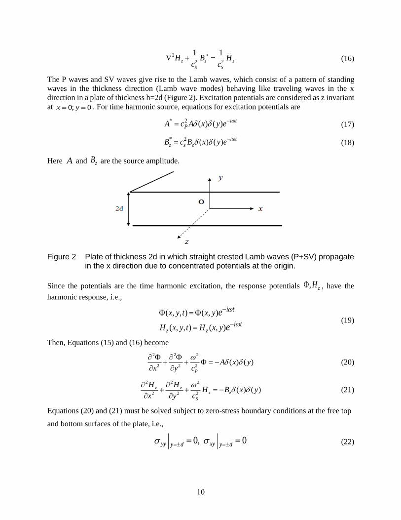
direction in a plate of thickness h=2d (Figure 2). Excitation potentials are considered as z invariant
at 0; 0x y . For time harmonic source, equations for excitation potentials are
* 2 ( ) ( ) i t
PA c A x y e (17)
* 2 ( ) ( ) i tz s zB c B x y e (18)
Here A and zB are the source amplitude.
Figure 2 Plate of thickness 2d in which straight crested Lamb waves (P+SV) propagate in the x direction due to concentrated potentials at the origin.
Since the potentials are the time harmonic excitation, the response potentials , zH , have the
harmonic response, i.e.,
( , , ) ( , )
( , , ) ( , )z z
i t
i t
x y t x y
H x y t H x y
e
e
(19)
Then, Equations (15) and (16) become
2 2 2
2 2 2( ) ( )
P
A x yx y c
(20)
2 2 2
2 2 2( ) ( )z z
z z
S
H HH B x y
x y c
(21)
Equations (20) and (21) must be solved subject to zero-stress boundary conditions at the free top
and bottom surfaces of the plate, i.e.,
0, 0yy xyy d y d
(22)

11
3 SOLUTION IN TERMS OF DISPLACEMENT
Taking Fourier transform of Equations (20) and (21), in x direction, ( , ) ( , )x y y and
( , ) ( , )H x y H y
2
2
2( , ) ( , ) ( , ) ( )
p
y y y A yc
(23)
2
2
2( , ) ( , ) ( , ) ( )z z z z
S
H y H y H y B yc
(24)
Here, ( ) ( )[ ( ) ]i xA y A y x e dx
and ( ) ( )[ ( ) ]i x
z zB y B y x e dx
Upon rearranging
2( , ) ( , ) ( )py y A y (25)
2( , ) ( , ) ( )z s z zH y H y B y (26)
Here,
22 2
2
22 2
2
p
p
s
s
c
c
(27)
Equations (25) and (26) are the second order ordinary differential equation (ODE) in y direction.
The total solution of Equations (25) and (26) consists of representation of two solutions [47]:
(a) The complementary solution for the homogeneous equation
(b) A particular solution of that satisfies source effect
Solution can be assumed as
0 1( , ) ( , ) ( , )y y y (28)
0 1( , ) ( , ) ( , )z z zH y i H y H y (29)
The functions 0 and 0zH satisfy the corresponding homogeneous differential equations
2
0 0( , ) ( , ) 0py y (30)
2
0 0( , ) ( , ) 0z s zH y H y (31)
Equations (30) and (31) give the complementary solutions, i.e.,

12
0 1 2( , ) C sin C cosp py y y (32)
0 1 2( , ) D sin D cosz s sH y y (33)
The functions 1( , )y and 1( , )zH y from Equation (29) satisfy the corresponding
inhomogeneous equations
2
11 1( , ) ( , ) ( ) ( )py y A y y (34)
2
1 1( , ) ( , ) ( ) ( )z s z zH y H y B y y (35)
Here, 1( , )y and 1( , )zH y are the Fourier transform of the free field depth dependent function.
The solution of Equation (34) is obtained using Fourier transform in y direction
2 2
1 1( , ) ( , )p A (36)
Here, ( ) i yA A y e dy
2 2
( , )p
A
(37)
The solution of Equation (35) is obtained in a similar way
2 2
1 1( , ) ( , )z s z zH H B
1 2 2( , ) z
z
s
BH
(38)
In order to get the solution in y domain, taking inverse Fourier transform of Equations (37) and
(38), i.e.,
1 2 2
1( , )
2
i y
p
Ay e d
(39)
1 2 2
1( , )
2
i yzz
s
BH y e d
(40)
The evaluation of the integral in Equations (39) and (40) can be done by the residue theorem using
a close contour [48]-[52] [Appendix B]. Integration formula for Equations (39) and (40) are
1 2 2
1( , ) sin
2 2
i y
p
p p
A Ay e d y
(41)
1 2 2
1( , ) sin
2 2
i yz zz s
s s
B BH e d y
(42)
13
Equations (41), (42) represent the particular solution. The total solution is superposition of
complementary solution Equations (32), (33) and particular solution Equations (41), (42), i.e.,
1 2( , ) C sin C cos sin2
p p p
p
Ay y y y
(43)
1 2( , ) D sin D cos sin
2
zz s s s
s
BH y i y y y
(44)
The coefficients 1 2 1 2C , C , D , D of the complimentary solutions Equations (32), (33) are to be
determined by using the Fourier transformed boundary conditions i.e.,
0, 0yy xyy d y d
(45)
After applying the boundary conditions [Appendix A: Equations (A20)-(A29)] we get
2 2
1 2
1 2
( ) C sin C cos sin2
2 D cos D sin cos2
0
s p p p
p
zs s s s s s
s
Ad d d
Bdd d
(46)
2 2
1 2
1 2
( ) C sin C cos sin2
2 D cos D sin cos2
0
s p p p
p
z
s s s s s s
s
Ad d d
Bdd d
(47)
1 2
2 2
1 2
2 C cos C sin cos2
( ) D sin D cos sin 02
p p p p p p
p
s s s
zs
s
Ad d d
d dB
d
(48)
1 2
2 2
1 2
2 C cos C sin cos2
( ) D sin D cos sin 02
p p p p p p
p
s s s
zs
s
Ad d d
d dB
d
(49)
Equations (46)-(49) are a set of four equations with four unknowns. The equations can be separated
into a couple of two equations with two unknowns, one for symmetric motion and one for anti-
symmetric motion.

14
3.1 SYMMETRIC LAMB WAVE SOLUTION
Addition of the Equations (46) and (47), and subtraction of the Equations (48) from(49), yields
2 2 2 2
2 2
2
1
( ) 2 ( )
2 ( )
cos cos C sin cos2
sin sin D0
s s
s
p s s p z s
pp p sd
Ad d d B d
d
(50)
Equation (50) represents an algebraic system that can be solved for 2C , 1D provided the system
determinant does not vanish
2 2
2 2
( )cos 2 cos0
2 sin ( )sin
s p s s
p p s s
s
d d
dD
Let,
2 2
( ) sin cos2
sS p z s
p
PA
d B d
(51)
SP is the source term for the symmetric solution which contains source potentials A and ZB .
Then,
2 2
2 2
2
1
( ) 2
2 ( )
sin cos
sin cos 0C
D
s
s
s
s s s S
p p pd
D
d d P
d
(52)
2 2
2
1
( )sin1
2 sin
C
D
S s s
S p ps
P d
P dD
(53)
Here,
2 2
2 2 2 2
2 2
( )cos 2 cos( ) cos sin 4 cos sin
2 sin ( )sin
s p s s
s p s s p s p
p p s s
s
d dd d d d
dD
(54)
By equating to zero the ( )sD term of Equation (54), one gets the symmetric Rayleigh -Lamb
equation.
3.2 ANTI-SYMMETRIC LAMB WAVE SOLUTION
Subtraction of the Equations (46) from(47), and addition of the Equations (48) and (49), yields
2 2
2 2 2 2
1
2
( ) 2
2 ( ) ( )
0sin sin C
cos cos D cos sin2
s
s s
p s s
zp p s p s
s
d dB
d A d d
(55)
15
Equation (55) represents an algebraic system that can be solved for 1C , 2D provided the system
determinant does not vanish
2 2
2 2
( )sin 2 sin0
2 cos ( )cos
s p s s
p p s s
A
d d
dD
Let,
2 2cos ( ) sin
2
zA p s s
s
BP A d d
(56)
AP is the source term for the anti-symmetric solution which contains source potentials A and ZB
.
Then,
2 2
2 2
1
2
( ) 2
2 ( )
cos sin 0
cos sinC
D
s
s
A
s s s
p p p Ad
D
d d
d P
(57)
2 2
1
2
2 sin1
( )sin
C
D
A s s
A s pA
P d
P dD
(58)
Here,
2 2
2 2 2 2
2 2
( )sin 2 sin( ) sin cos 4 sin cos
2 cos ( )cos
s p s s
s p s s p s p
p p s s
A
d dd d d d
dD
(59)
By equating to zero the ( )AD term of Equation (59), one gets the anti-symmetric Rayleigh -
Lamb equation.
3.3 DISPLACEMENT SOLUTION IN THE WAVENUMBER DOMAIN
Equation (A14) [Appendix A] gives the out-of-plane displacement yu , in terms of potentials, i.e.,
z
y
Hu
y x
(60)
In ‘x’ direction wavenumber domain the displacement yu becomes
y zu i Hy
(61)
By substituting of Equations (43), (44) into Equation (61) yields the expressions for out-of-plane
displacement in the wavenumber domain in terms of coefficients 1 2 1 2C , C , D , D which are
functions of the wavenumber ξ, i.e.,
16
1 2 1 2C cos C sin D sin D cos cos sin2 2
zy p p p p s s p s
s
BAu y y y y d d
(62)
Evaluation of Equation (62) at the plate top surface, y y d
u
:
1 2 1 2C cos C sin D sin D cos cos sin2 2
zy p p p p s s p s
s
BAu d d d d d d
(63)
The complete solution of displacement is the superposition of the symmetric, antisymmetric and
bulk wave solution. By using Equations (53) and (58) into Equation (63) and obtain
cos sin2 2
S A zy S A p s
S A s
N N BAu P P d d
D D
(64)
Where,
2 2 2
2 2
2 sin sin ( ) sin sin
2 sin cos ( )sin cos
s p p s s p p s
A s p s p s p s
N d d d d
N d d d d
(65)
3.4 DISPLACEMENT SOLUTION IN THE PHYSICAL DOMAIN
Displacement solution in the physical domain is obtained by taking inverse Fourier transform of
Equation (64), i.e.,
1
cos sin2 2 2
i xS A zy S A p s
S A s
N N BAu P P d d e d
D D
(66)
Let,
1 2 3yu I I I (67)
Where,
1
1
2
i xS AS A
S A
N NI P P e d
D D
(68)
2
1cos
2 2
i x
p
AI d e d
(69)
3
1sin
2 2
i xzs
s
BI d e d
(70)
The integration of Equations (68), (69), (70) are presented in Appendix C. After integrating
Equations (68), (69), (70), the displacement yu becomes

17
1 11 1
2 2 2 2 2 2 2 22 22 21 0
0 0
Y ( ) J ( )4 2
(2
( )( )( ) ( )
( ) ( )
As AS j jj
j
y
z
P p S S
z
AS jji xAi xjSS A
j jS AS Aj js j A
u
BAd x d x d x x d x d
c c c c
iB
NNi P e P e
D D
1 1
2 2 2 22 21) ( ) Y ( )( )
S S
x x d x dc c
(71)
After rearranging Equation (71) and reinstating explicitly the harmonic time dependency, we get,
1 11 1
2 2 2 2 2 2 2 22 22 21 0
( )( )
0 0
Y ( ) J ( )4 2
( )( )( ) ( )
( ) ( )
As AS j jj
j
y
i t i tz
P P S S
AS jji x tAi x tjSS A
j jS AS Aj js j A
u
BAd x d x d e x x d x d e
c c c c
i
NNi P e P e
D D
1 1
2 2 2 22 21( ) ( ) Y ( )( )
2
i tz
S S
Bx x d x d e
c c
(72)
Assume that,
y y L y A y Bu u u u
Where,
( )( )
0 0
( )( )( ) ( )
( ) ( )
As AS j jj
j
y L
AS jji x tAi x tjSS A
j jS AS Aj js j A
uNN
i P e P eD D
(73)
1
2
1 12 2 2 22 2
1J4
i t
y A
p p
Au x d x d d x e
c c
(74)
1 1
2 2 2 22 20
1 1
2 2 2 22 21
( ) J ( )2
( ) ( ) Y ( )( )2
i tzy B
S S
i tz
S S
Bu x x d x d e
c c
iBx x d x d e
c c
(75)
y Lu is the out-of-plane displacement containing Lamb wave mode and ,y A y Bu u are the out-of-plane
displacements of bulk wave for excitation potentials A and zB respectively.
Theoretical derivation reveals that, bulk wave is present in addition to Lamb wave. The Lamb
waves, which consist of a pattern of standing waves in the thickness direction (Lamb wave modes)

18
behaving like traveling waves in the x direction in a plate. Guided waves can propagate long
distances, yields an easy inspection of a wide variety of structures. Whereas, bulk waves generate
from a source and directly reach to the AE sensor without interfering the boundaries. Bulk waves
are categorized into longitudinal (pressure) and transverse (shear) waves. The displacements y Au
and y Bu are the longitudinal and transverse bulk waves respectively.
3.5 EFFECT OF SOURCE DEPTH
If the source is present at different location other than mid-plane i.e., 0y y (Figure 3) then
equations for excitation potentials become
* 2
0( ) ( ) i tpA c A x y y e (76)
* 2
0( ) ( ) i tz s zB c B x y y e (77)
Recall Equations (25) and (26) for new location of excitation potentials
2
0( , ) ( , ) ( )py y A y y (78)
2
0( , ) ( , ) ( )z s z zH y H y B y y (79)
Complementary solution of Equation (78) and (79) will be the same as before. Only particular
solution will change due to the source in right hand side.
Figure 3 Plate of thickness 2d in which straight crested Lamb waves (P+SV) propagate
in the x direction due to concentrated potentials at 0y y
Fourier shift transform states that,
0
0{ ( )} { ( )}i y
F f y y e F f y
(80)
By using Fourier shift transform theorem Equation (80), the particular solutions of Equations (78)
, (79) become
0
1 2 2
1( , )
2
i yi y
p
Aey e d
(81)

19
0
1 2 2
1( , )
2
i yi yz
z
s
B eH y e d
(82)
Upon rearranging,
0( )
1 2 2
1( , )
2
i y y
p
Ay e d
(83)
0( )
1 2 2
1( , )
2
i y yzz
s
BH y e d
(84)
Integration of Equations (83) and (84) can be done by using residue theorem. The detailed solution
is already presented before from Equations (39) to (42). For brevity, only the final results of
Equations (83), (84) are presented here. From residue theorem the integrands become,
0( )
1 02 2
1( , ) sin
2 2
i y y
p
p p
A Ay e d y y
(85)
Similarly,
0( )
1 02 2
1( , ) sin
2 2
i y yz zz s
s s
B BH e d y y
(86)
The corresponding source terms, Equations (51) and (56) for symmetric and antisymmetric
solutions will be
2 2
1 1( ) sin cos2
S s p z s
p
AP d B d
(87)
2 2
1 1cos ( ) sin2
zA p s s
s
BP A d d
(88)
Here, 1 0d d y
The corresponding displacement Equations (73), (74), (75) become
( )( )
0 0
( )( )( ) ( )
( ) ( )
As AS j jj
j
y L
AS jji x tAi x tjSS A
j jS AS Aj js j A
uNN
i P e P eD D
(89)
1 1
2 2 2 22 21 1 1Y
4 p p
i tc cy A
Au x d x d e
(90)
1 1
2 2 2 22 21 0 1
1 1
2 2 2 22 21 1 1
( ) J ( )2
( ) ( ) Y ( )( )2
s s
s s
i tzc cy B
i tzc c
Bu x x d x d e
iBx x d x d e
(91)

20
3.6 AE GUIDED WAVE PROPAGATION
AE guided waves will be generated by the AE event. AE guided waves will propagate through the
structure according to the structural transfer function. The out-of-plane displacement of the guided
waves can be captured by conventional AE transducer installed on the surface of the structure as
shown in Figure 4.
Figure 4 Acoustic emission propagation and detection by a sensor installed on a structure
For numerical analysis, a 304-stainless steel plate with 6 mm thickness was chosen as a case study.
The signal was received at 500 mm distance from the source. The excitation source was located at
the mid-plane of the plate. A very short peak time of 3 s was used for this case study. Later, the
effects of source depth and propagation distance were included into the study. A detailed
methodology of the numerical analysis is described in Figure 5. In numerical analysis, direct
Fourier transforms of the time domain excitation signal was performed to get the frequency
contents of the signal and an inverse Fourier transform was done to get the time domain output
signal from frequency response of out-of-plane displacement.

21
Figure 5 Methodology for guided wave analysis

22
4 NUMERICAL STUDIES
This section includes guided wave simulation in a plate due to excitation potentials.
4.1 TIME DEPENDENT EXCITATION POTENTIALS
The time-dependent excitation potentials depend on time-dependent energy released from a crack.
A real AE source releases energy during a finite time period. At the beginning, the rate of energy
released from a crack increases sharply with time and reaches a maximum peak value within very
short time; then decreases asymptotically toward the steady state value, usually zero. Time rate of
energy released from a crack can be modeled as a Gaussian pulse. Figure 6a and Figure 7a show
the time rate of pressure potential and shear potential. The corresponding equations are,
2
2
2
2*
2
0
*2
0
t
zZ
tA
A t et
BB t e
t
(92)
Here 0A and 0ZB are the scaling factors. Time profile of the potentials are to be evaluated by
integrating Equation (92), i.e.,
2
2
2
2
0
0
( ) 2
( ) 2
t
t
z z
tA A erf te
tB B erf te
(93)
Figure 6 (a) Time rate of pressure potential *A t and (b) Time profile of pressure
potential ( *A )

23
Figure 7 (a) Time rate of shear potential *
zB t and (b) Time profile of shear potential
*( )zB
Time profile of potential is shown in Figure 6b and Figure 7b. Time profile of AE source may
follow cosine bell function [37], [38] or error function. In this research, a Gaussian pulse is used
to model the growth of the excitation potentials during the AE event; as a result, the actual
excitation potential follows the error function variation in the time domain. Cuadra et al. [33]
obtained similar time profile of AE energy from a crack by using 3D computation method.
The key characteristics of the excitation potentials are:
peak time: time required to reach the time rate of potential to maximum value
rise time: time required to reach the potential to 98% of maximum value or steady state
value
peak value: maximum value of time rate of potential
maximum potential: maximum value of time profile of potential
Amplitude of the source A and zB for unit width is,
2
2
2
2
02
02
( ) 2
( ) 2
t
p
t
z z
s
h tA A erf tec
h tB B erf tec
(94)
Here, plate thickness 2h d .

24
4.2 PHASE VELOCITY AND GROUP VELOCITY DISPERSION CURVES
Solution of the Rayleigh-Lamb equation for symmetric and antisymmetric modes (Equations (54)
and (59)) yields the wave number and hence the phase velocity for each given frequency. Multiple
solutions exist, hence multiple Lamb modes also exist. Differentiation of phase velocity with
respect to frequency yields the group velocity. The phase velocity dispersion curves and group
velocity dispersion curves are shown in Figure 8a and Figure 8b respectively. The existence of
certain Lamb mode depends on the plate thickness and frequency. The fundamental S0 and A0
modes will always exist. The phase velocity (Figure 8a) is associated with the phase difference
between the vibrations observed at two different points during the passage of the wave. The phase
velocity is used to calculate the wave length of each mode.
(a) (b)
Figure 8 Lamb wave dispersion curves: (a) phase velocity and (b) group velocity of symmetric and anti-symmetric Lamb wave modes.
The fundamental wave mode of symmetric (S0) and anti-symmetric (A0) is considered in this
analysis. The signal is received at some distance away from the point of excitation potentials, only
the modes with real-valued wavenumbers are included in the simulation. The corresponding modes
for imaginary and complex-valued wavenumbers are ignored because they propagate with
decaying amplitude; at sufficiently far from the excitation point their amplitudes are negligible.
Since different Lamb wave modes traveling with different wave speeds exist simultaneously, the
excitation potentials will generate S0 and A0 wave packets. The group velocity (Figure 8b) of
Lamb waves is important when examining the traveling of Lamb wave packets. These wave
packets will travel independently through the plate and will arrive at different times. Due to the
multi-mode character of guided Lamb wave propagation, the received signal has at least two
separate wave packets, S0 and A0 All wave modes propagate independently in the structure. The
final waveform will be the superposition of all the propagating waves and will have the
contribution from each Lamb wave mode.
4.3 EXAMPLE OF AE GUIDED WAVE PROPAGATION IN A 6MM PLATE
A test case example is presented in this section to show how AE guided waves propagate over a
certain distance using excitation potentials. A 304-stainless steel plate with 6 mm thickness was
chosen for this purpose. The signal was received at a distance 500 mm away from the source.
Excitation sources were located at mid-plane of the plate ( 1 3 mmd ). Time profile excitation
potentials (Figure 6b and Figure 7b) were used to simulate AE waves in the plate. Excitation

25
potential can be calculated from the time rate of potential released during crack propagation. Peak
time, rise time, peak value and maximum potential of excitation potentials are 3 s , 6.6 s , 0.28
W/kg and 1 J/kg . Based on this information a numerical study on AE Lamb wave propagation
was conducted. Peak time or rise time is one of the major characteristics of AE source. Several
researchers investigate potential effect of rise time on AE signal by varying the source rise time
in-between 0.1 s to 15 s [37]- [39], [55].
(a) Pressure potential excitation (b) Shear potential excitation
Figure 9 Lamb waves (S0 and A0 mode) and bulk waves propagation at 500 mm distance in 6 mm 304-steel plate for (a) pressure potential excitation (b) shear potential excitation (peak time = 3 s ) located at mid plane.
In this research, each excitation potential was considered separately to simulate the Lamb waves.
Total released energy from a crack can be decomposed to pressure and shear excitation potentials.
This research presents the individual effect of the unit amplitude of potentials (1 J/kg ) on AE
signals. However, distributing the energy between the pressure and shear potentials for real AE

26
source is very important and we recommend it for future study for specific damage assumptions
(e.g., a crack propagating under Mode I fracture may have a different mix of shear/pressure
potentials than a crack propagating under Mode II or Mode III fracture modes; similarly for mixed-
mode fracture).
Figure 9a shows the Lamb wave (S0 and A0 mode) and bulk wave propagation using pressure
excitation potential. Signals are normalized by their individual peak amplitudes, i.e., amplitude/
peak amplitude. It can be inferred from the figures that both A0 and S0 are dispersive. Bulk wave
shows nondispersive behavior, but the peak amplitude is not significant compared to peak S0 and
A0 amplitude. Figure 9b shows the Lamb wave (S0 and A0 mode) and bulk wave propagation
using shear potential only. Peak amplitude of A0 is higher than peak S0 amplitude while using
shear potential only (Figure 9b). By comparing Figure 9a and Figure 9b the important observation
can be made as, pressure excitation potential has more contribution to the peak S0 amplitude over
shear excitation potentials whereas, shear excitation potential has more contribution to the peak
A0 amplitude. The notable characteristic is that, peak amplitude of A0 is higher than the peak S0
amplitude for both excitation potentials. It should be noted that, the peak amplitude of the bulk
wave is much smaller than the peak A0 and S0 amplitudes for both pressure and shear excitation
potentials located at the mid-plane. But their contribution to the S0 and A0 peak amplitude might
change due to change in source depth and propagating distance. The following sections discuss
the effect of source depth, higher propagating mode and propagating distance in AE guided wave
propagation using excitation potentials.
4.4 EFFECT OF SOURCE DEPTH
To study the effect of source depth, a 6 mm thick plate was chosen. The signal was received at 500
mm distance from the source. The excitation sources were located at the top surface, 1.5 mm from
the top surface, and 3 mm from the top surface (mid plane). Figure 9, Figure 10, Figure 11 show
the out-of-plane displacement (S0 and A0 mode, bulk wave) vs time at 500 mm propagation
distance in 6mm thick plate for mid-plane, top surface and 1.5 mm depth from top surface source
location. The summary of the results are listed in Table 1. Signals are normalized by their
individual peak amplitudes, i.e., amplitude/ peak amplitude. From Figure 10 it is observed that,
the A0 mode appears only while using pressure potential on the top surface whereas, S0 mode
appears only while using shear potential. Therefore, pressure potential contributes to the peak A0
amplitude and shear potential contributes to the peak S0 amplitude in the final waveform. Another
notable characteristic is that, the pressure potential contributes to the high amplitude of the trailing
edge (low frequency component) of A0 wave packet for top-surface source. With increasing source
depth, the effect of high amplitude of low frequency decreases (Figure 9a and Figure 11a) in A0
signal. By comparing the amplitude scales of Figure 9 and Figure 11, the increase in peak A0
amplitude and the decrease in peak S0 amplitude with increasing source depth while using pressure
excitation potential only.
Figure 9b, Figure 10b and Figure 11b show some qualitative and quantitative changes in spectrum
while using shear excitation potentials only. The amplitude of S0 signal decreases and A0 signal
increases with increasing source depth while using shear excitation potential only (Figure 11b and
Figure 9b). Qualitative change in S0 signal with source depth refers to the change in frequency
content of the signal. It should be noted that, peak amplitude of S0 and A0 signal using shear
excitation potential located at 1.5 mm depth from the top surface is more significant compared to
pressure potential located at same location (Figure 11). However, with increasing source depth, S0

27
signals amplitude become more significant due to pressure excitation potential over shear
excitation potential (Figure 9 and Figure 11). For all AE source location, the shear potential part
of the AE source has more contribution to the peak A0 amplitude than pressure potential. Peak
amplitude of bulk waves increases with increasing source depth (Figure 9 and Figure 11).
However, the amplitude of bulk wave is much smaller than the peak A0 and S0 amplitudes.
Therefore, peak amplitude of bulk wave may not appear in real AE signal.
(a) Pressure potential excitation (b) Shear potential excitation
Figure 10 Lamb waves (S0 and A0 mode) and bulk waves propagation at 500 mm distance in 6 mm 304-steel plate for (a) pressure potential excitation (b) shear potential excitation (peak time = 3 s ) located on top surface.

28
(a) Pressure potential excitation (b) Shear potential excitation
Figure 11 Lamb waves (S0 and A0 mode) and bulk waves propagation at 500 mm distance in 6 mm 304-steel plate for (a) pressure potential excitation (b) shear potential excitation (peak time = 3 s ) located at 1.5 mm depth from top
surface.
Table 1 Comparison of peak amplitudes of Lamb waves (S0 and A0 mode) and bulk waves for different source depth
Source depth
Peak S0 amplitude
(m)
Peak A0 amplitude
(m)
Peak bulk wave amplitude
(m)
Pressure Shear Pressure Shear Pressure Shear
Top surface
source - 5.0e-15 7.3e-15 - - -
1.5 mm from
top surface 7.5e-16 3.8e-15 7.4e-15 1.07e-14 7.14e-19 2.37e-17
Mid-plane
source 2.5e-15 1.9e-15 1.6e-14 2.5e-14 1.43e-18 2.4e-17
29
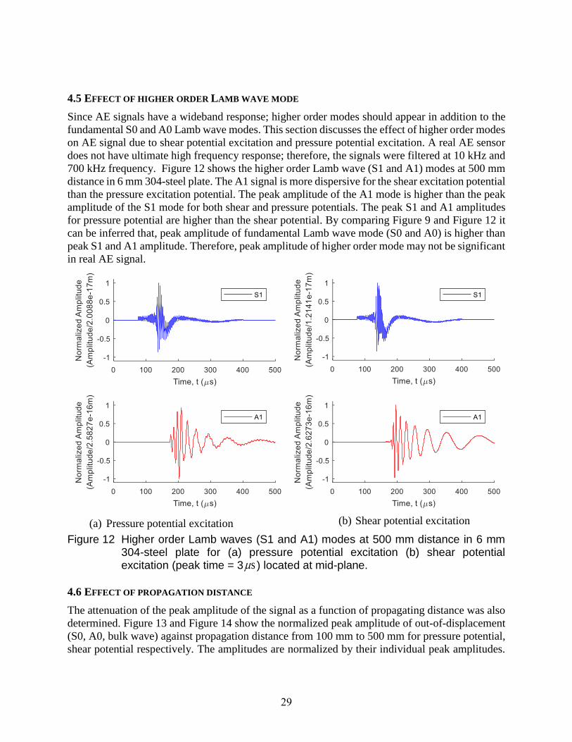
4.5 EFFECT OF HIGHER ORDER LAMB WAVE MODE
Since AE signals have a wideband response; higher order modes should appear in addition to the
fundamental S0 and A0 Lamb wave modes. This section discusses the effect of higher order modes
on AE signal due to shear potential excitation and pressure potential excitation. A real AE sensor
does not have ultimate high frequency response; therefore, the signals were filtered at 10 kHz and
700 kHz frequency. Figure 12 shows the higher order Lamb wave (S1 and A1) modes at 500 mm
distance in 6 mm 304-steel plate. The A1 signal is more dispersive for the shear excitation potential
than the pressure excitation potential. The peak amplitude of the A1 mode is higher than the peak
amplitude of the S1 mode for both shear and pressure potentials. The peak S1 and A1 amplitudes
for pressure potential are higher than the shear potential. By comparing Figure 9 and Figure 12 it
can be inferred that, peak amplitude of fundamental Lamb wave mode (S0 and A0) is higher than
peak S1 and A1 amplitude. Therefore, peak amplitude of higher order mode may not be significant
in real AE signal.
(a) Pressure potential excitation (b) Shear potential excitation
Figure 12 Higher order Lamb waves (S1 and A1) modes at 500 mm distance in 6 mm 304-steel plate for (a) pressure potential excitation (b) shear potential excitation (peak time = 3 s ) located at mid-plane.
4.6 EFFECT OF PROPAGATION DISTANCE
The attenuation of the peak amplitude of the signal as a function of propagating distance was also
determined. Figure 13 and Figure 14 show the normalized peak amplitude of out-of-displacement
(S0, A0, bulk wave) against propagation distance from 100 mm to 500 mm for pressure potential,
shear potential respectively. The amplitudes are normalized by their individual peak amplitudes.

30
A 6 mm thick 304-steel plate with both excitation potentials are considered. Potentials are located
at mid-plane with peak time of 3 s .
Figure 13 Effect of pressure excitation potential: variation of out-of-plane displacement (S0, A0 and bulk wave) with propagation distance in 6 mm 304- steel plate for source (peak time = 3 s ) located at the mid-plane.
Figure 14 Effect of shear excitation potential: variation of out-of-plane displacement (S0, A0 and bulk wave) with propagation distance in a 6-mm 304-steel plate for source (peak time = 3 s ) located at the mid-plane.
0
0.2
0.4
0.6
0.8
1
100 200 300 400 500
Ou
t o
f p
lan
e d
isp
lace
men
t
(Norm
aliz
ed p
eak a
mpli
tude)
Propagation distance (mm)
S0
A0
Bulk wave
0
0.2
0.4
0.6
0.8
1
100 200 300 400 500
Out
of
pla
ne
dis
pla
cem
ent
(Norm
aliz
ed p
eak a
mpli
tude)
Propagation distance (mm)
S0
A0
Bulk wave

31
Figure 13 and Figure 14 show significant attenuation of S0, A0, and bulk wave signal with
propagating distance 100 mm to 500 mm. However, larger attenuation of peak bulk wave
amplitude is observed compared to peak S0 and A0 amplitudes. Therefore, far from the source
bulk wave becomes less significant and may not be captured by the AE transducer. Another
important observation is that, peak A0 amplitude attenuates more than peak S0 amplitude while
using pressure potential only whereas, peak S0 amplitude attenuates more than peak A0 amplitude
while using shear potential only. The attenuation of the peak amplitude is expected due to
dispersion of the signal.
5 SUMMARY, CONCLUSIONS, AND FUTURE WORK
5.1 SUMMARY
The guided waves generated by an acoustic emission (AE) event were analyzed through a
Helmholtz potential approach. The inhomogeneous elastodynamic Navier-Lame equation was
expressed as a system of wave equations in terms of unknown scalar and vector solution potentials,
, H , and known scalar and vector excitation potentials, *A , *B . The excitation potentials *A , *B were traced to the energy released during an incremental crack propagation.
The solution was readily obtained through direct and inverse Fourier transforms and application
of the residue theorem. The resulting solution took the form of a series expansion containing the
superposition of all the Lamb waves modes and bulk waves existing for the particular frequency-
thickness combination under consideration.
A numerical study of the AE guided wave propagation in a 6 mm thick 304-steel plate was
conducted in order to predict the out-of-plane displacement that would be recorded by an AE
sensor placed on the plate surface at some distance away from the source. Parameter studies were
performed to evaluate: (a) the effect of the pressure and shear potentials; (b) the effect of the
thickness-wise location of the excitation potential sources varying from mid-plane to the top
surface (source depth effect); (c) the effect of higher propagating mode; (d) the effect of
propagating distance away from the source.
5.2 CONCLUSIONS
The present work has shown that pressure and shear source potentials can be used to model the
guided wave generation and propagation due to an AE event associated with incremental crack
growth. The advantage of this approach is to decouple the inhomogeneous Navier-Lame equations.
The numerical studies performed over a range of parameters have shown that:
i. Both A0 and S0 modes generated by an AE excitation in a 6-mm steel plate are
dispersive. The high frequency components of the AE excitation are responsible for the
dispersive part of the S0 mode, whereas the low frequency components of the AE
excitation are responsible for the dispersive part of the A0 mode.
ii. The peak amplitude of A0 mode is higher than the peak amplitude of the S0 mode for
all cases.
iii. The amplitude of bulk wave is much smaller than peak A0 and S0 amplitude.
Therefore, peak amplitude of bulk waves may not be significant in real AE signal.
iv. For mid-plane AE source location, the shear potential part of the AE source has more
contribution to the peak A0 amplitude than pressure potential whereas the pressure

32
potential part of the AE source has more contribution to the peak S0 amplitude than
shear potential.
v. With an increase in the source depth, the peak A0 and S0 amplitude increases by
considering pressure potential only, whereas, the peak A0 increases and S0 decreases
by using shear potential only.
vi. If the AE source is located at top surface, the effect of the excitation pressure and shear
potentials on the S0 and A0 modes seems to be decoupled: pressure potential does not
contribute to S0 and bulk wave amplitude whereas shear potential does not contribute
to the A0 and bulk wave amplitude.
vii. For top-surface AE source, pressure excitation potential has contribution to the high
amplitude low-frequency component of the A0 wave packet. This contribution
decreases as the source depth increases.
5.3 FUTURE WORK
Substantial future work is still needed to verify the hypotheses and substantiate the calculation of
the AE source potentials that produce the guided wave excitation. The extensive experimental AE
monitoring data existing in the literature should be explored to find actual physical signals that
could be compared with numerical predictions in order to extract factual data about the amplitude
and time-evolution of the AE source potentials. A frequency analysis of time domain signal should
be done to analyze the frequency content of the captured AE signals. Frequency content may help
to distinguish different source types and source location. If necessary, additional experiments with
wider band AE sensors should be conducted. An inverse algorithm could then be developed to
characterize the AE source during crack propagation. The source characterization can provide
information about amount of energy released from the crack. Therefore, it may help to generate a
qualitative as well quantitative description of the crack propagation phenomenon. A further
extensive study on the effect of plate thickness, AE rise time, and AE source depth would be
recommended.
Straight crested Lamb wave (1-D wave guided propagation) was considered in this paper.
However, realistic AE guided wave propagation usually takes place events in 2D geometries
(pressure vessels, containment vessels, etc.). Hence, the present theory should be extended to
circular crested Lamb waves (2-D wave guided propagation). The contribution of pressure and
shear excitation potentials to the total energy release from a crack needs to be studied through
types of materials and crack types.
ACKNOWLEDGEMENT
The authors are grateful for the financial support from US Department of Energy (DOE), Office
of Nuclear Energy, under grant numbers DE-NE 0000726 and DE-NE 0008400.

33
REFERENCES
[1] Harris, D. O. and Dunegan, H. L. (1974) “Continuous monitoring of fatigue-crack
growth by acoustic-emission techniques,” Experimental Mechanics, 14(2), 71-81.
[2] Han, B. H., Yoon, D. J., Huh, Y. H. and Lee, Y. S. (2014) “Damage assessment of wind
turbine blade under static loading test using acoustic emission,” Journal of Intelligent
Material Systems and Structures, 25(5), 621-630.
[3] Tandon, N. and Choudhury, A. (1999) “A review of vibration and acoustic measurement
methods for the detection of defects in rolling element bearings,” Tribology
International, 32(8), 469-480.
[4] Roberts, T. and Talebzadeh, M. (2003) “Acoustic emission monitoring of fatigue crack
propagation,” Journal of Constructional Steel Research, 59(6), 695-712.
[5] Bassim, M. N., Lawrence, S. S. and Liu, C. D. (1994) “Detection of the onset of fatigue
crack growth in rail steels using acoustic emission,” Engineering Fracture Mechanics,
47(2), 207-214.
[6] Lamb, H. (1917, March) “On waves in an elastic plate,” In Proceedings of the Royal
Society of London A: Mathematical, Physical and Engineering Sciences (Vol. 93, No.
648, pp. 114-128), The Royal Society.
[7] Helmholtz, H. (1858) “Uber Integrale der Hydrodynamischen Gleichungen, Welche den
Wirbelbewegungen Entsprechen,” J. fur die reine und angewandte Mathematik, vol.
1858, no. 55, pp. 25–55, 1858. (https://eudml.org/doc/147720)
[8] Achenbach, J. D. (2003) Reciprocity in elastodynamics, Cambridge University Press.
[9] Giurgiutiu, V. (2014) Structural Health Monitoring with Piezoelectric Wafer Active
Sensors, 2nd edition, New York: Academic, ISBN: 9780124186910.
[10] Graff, K. F. (1975) Wave motion in elastic solids, Courier Corporation.
[11] Viktorov, I. A. (1967) Rayleigh and Lamb Waves: Physical Theory and Applications,
Transl. from Russian. with a Foreword by Warren P. Mason. Plenum Press.
[12] Landau, L. D., and Lifschitz, E. M. (1965) Teoriya uprugosti, Nauka, Moscow, 1965
(Theory of Elasticity, 2nd ed., Pergamon Press. Oxford, 1970).
[13] Love, A. E. H. (1944) A treatise on the mathematical theory of elasticity, New York:
Dover.
[14] Aki, K., & Richards, P. G. (2002) Quantitative seismology (Vol. 1).
[15] Vvedenskaya, A. V. (1956) “The determination of displacement fields by means of
dislocation theory,” Izvestiya Akas, Nauk, SSSR, 227-284.
[16] Nabarro, F. R. N., (1951) Phil. Mag. 42:313.
[17] Maruyama, T. (1963). “On the force equivalents of dynamical elastic dislocations with
reference to the earthquake mechanism,” Bull. Earthq. Res. Inst., Tokyo Univ., 41,467–
486.
[18] Lamb, H. (1903) “On the Propagation of Tremors over the Surface of an Elastic Solid,”
Proceedings of the royal society of London, 72, 128-130.
[19] Rice, J. R. (1980) “Elastic wave emission from damage processes,” Journal of
Nondestructive Evaluation,” 1(4), 215-224.
[20] Miklowitz, J., (1962) “Transient compressional waves in an infinite elastic plate or

34
elastic layer overlying a rigid half-space,” J. Appl. Mech. 29, 53–60.
[21] Weaver, R. L. and Pao, Y.-H. (1982) “Axisymmetric elastic waves excited by a point
source in a plate,” J. Appl. Mech. 49, 821–836.
[22] Ono, K., and Ohtsu, M. (1984) “A generalized theory of acoustic emission and Green's
functions in a half space,” Journal of Acoustic Emission, 3, 27-40.
[23] Ohtsu, M., & Ono, K. (1986) “The generalized theory and source representations of
acoustic emission,” Journal of Acoustic Emission, 5(4), 124-133.
[24] Johnson, L. R. (1974) “Green's function for Lamb's problem,” Geophysical Journal
International, 37(1), 99-131.
[25] Roth, F. (1990) “Subsurface deformations in a layered elastic half-space,” Geophysical
Journal International, 103(1), 147-155.
[26] Bai, H., Zhu, J., Shah, A. H. and Popplewell, N. (2004) “Three-dimensional steady state
Green function for a layered isotropic plate,” Journal of Sound and Vibration, 269(1),
251-271.
[27] G.R. Liu and J.D. Achenbach (1995) “Strip element method to analyze wave scattering
by cracks in anisotropic laminated plates,” Journal of Applied Mechanics, American
Society of Mechanical Engineers, 62 (1995) 607–613.
[28] Jacobs, L. J., Scott, W. R., Granata, D. M. and Ryan, M. J. 1991. “Experimental and
analytical characterization of acoustic emission signals. Journal of nondestructive
evaluation, 10(2), 63-70.
[29] Ono, K. 2011. Acoustic emission in materials research–A review. Journal of acoustic
emission, 29, 284-309.
[30] Wisner, B., Cabal, M., Vanniamparambil, P. A., Hochhalter, J., Leser, W. P. and
Kontsos, A. 2015. In situ microscopic investigation to validate acoustic emission
monitoring. Experimental Mechanics, 55(9), 1705-1715.
[31] Momon, S., Moevus, M., Godin, N., R’Mili, M., Reynaud, P., Fantozzi, G., & Fayolle,
G. (2010). Acoustic emission and lifetime prediction during static fatigue tests on
ceramic-matrix-composite at high temperature under air. Composites Part A: Applied
Science and Manufacturing, 41(7), 913-918.
[32] Haider, M. F., Giurgiutiu, V., Lin, B., and Yu, L. (2017). Irreversibility effects in
piezoelectric wafer active sensors after exposure to high temperature. Smart Mater.
Struct, 26(095019), 095019.
[33] Cuadra, J. A., Baxevanakis, K. P., Mazzotti, M., Bartoli, I. and Kontsos, A. 2016.
Energy dissipation via acoustic emission in ductile crack initiation, International Journal
of Fracture, 199(1), 89-104.
[34] Khalifa, W. B., Jezzine, K., Grondel, S., Hello, G., & Lhémery, A. (2012). Modeling of
the Far-field Acoustic Emission from a Crack under Stress. Journal of Acoustic
Emission, 30, 137-152.
[35] Hamstad, M. A., O'GALLAGHER, A. and Gary, J. (1999) “Modeling of buried
monopole and dipole sources of acoustic emission with a finite element technique,”
Journal of Acoustic Emission, 17(3-4), 97-110.
[36] Hill, R., Forsyth, S. A. and Macey, P. (2004) “Finite element modelling of ultrasound,
with reference to transducers and AE waves,” Ultrasonics, 42(1), 253-258.

35
[37] Hamstad, M. A. (2010) “Frequencies and amplitudes of AE signals in a plate as a
function of source rise time,” In Proceeding of the 29th European Conference on
Acoustic Emission Testing.
[38] Sause, M. G., Hamstad, M. A. and Horn, S. (2013). Finite element modeling of lamb
wave propagation in anisotropic hybrid materials. Composites Part B: Engineering, 53,
249-257.
[39] Michaels, J. E., Michaels, T. E. and Sachse, W. (1981) “Applications of deconvolution
to acoustic emission signal analysis,” Materials Evaluation, 39(11), 1032-1036.
[40] Hsu, N. N., Simmons, J. A. and Hardy, S. C. (1978) “Approach to Acoustic Emission
Signal Analysis-Theory and Experiment,” Proceedings of the ARPA/AFML Review of
Progress in Quantitative NDE, September 1976–June 1977. 31.
[41] Pao, Y. H. (1978) Theory of acoustic emission, umu7i, 389.
[42] Ohtsu, M. (1995) “Acoustic emission theory for moment tensor analysis,” Journal of
Research in Nondestructive Evaluation, 6(3), 169-184.
[43] Fischer-Cripps, A. C. (2000) Introduction to contact mechanics, New York: Springer.
[44] Wolski, A. (2011) “Theory of electromagnetic fields,” arXiv preprint arXiv:1111.4354.
[45] Jackson, J. D. (1999) Classical electrodynamics, Wiley.
[46] Uman, M. A., McLain, D. K. and Krider, E. P. (1975) “The electromagnetic radiation
from a finite antenna,” Am. J. Phys, 43(1), 33-38.
[47] Jensen, F. B., Kuperman, W. A., Porter, M. B. and Schmidt, H. (2011) Computational
ocean acoustics, Springer Science & Business Media.
[48] Remmert, R. (2012) Theory of complex functions (Vol. 122). Springer Science &
Business Media.
[49] Cohen, H. (2010) Complex analysis with applications in science and engineering,
Springer Science & Business Media.
[50] Krantz, S. G. (2007) Complex Variables: a physical approach with applications and
MATLAB, CRC Press.
[51] Watanabe, K. (2014) Integral transform techniques for Green's function, New York:
Springer.
[52] Breckenridge, F. R., Proctor, T. M., Hsu, N. N., Fick, S. E. and Eitzen, D. G. (1990)
“Transient sources for acoustic emission work,” Progress in acoustic emission V, 20-
37.
[53] Erdélyi A (ed) (1954) Tables of integral transforms, vol II. McGraw-Hill, New York
[54] Bailey, W. N. (1938) “Some integrals involving Bessel functions,” The Quarterly
Journal of Mathematics, Oxford series, 9, 141-147.
[55] Haider, M. F., Giurgiutiu, V., Lin, B. and Yu, Y. (2017) Simulation of Lamb Wave
Propagation using Excitation Potentials, ASME 2017 Pressure Vessels & Piping
Conference, July 17, 2017, Waikoloa, Hawaii, United States, PVP2017-66074.

36
APPENDIX A
WAVE EQUATIONS FOR POTENTIALS
Recall the inhomogeneous Navier-Lame equations in vector form
2( ) u u f u (A1)
Upon substitution of Equations (5), (8) into Equation (A1), Equation (A1) becomes,
2 2 2( ) ( ) ( ) ( ) ( )H A B H (A2)
Upon rearrangement of Equation (A2)
2 2[( 2 )( ) - ] ( ) 0A H B H (A3)
For Equation (A3) to hold at any place and any time, the components in parentheses must be
independently zero, i.e.,
2( 2 )( ) - 0A (A4)
2 0H B H (A5)
Upon division by and rearrangement,
2 2
Pc A (A6)
2 2
Sc H B H (A7)
Here, 2 2
;Pc
2
Sc
Equation (A6) and (A7) are the wave equations for the scalar potential and the vector potential
respectively.
The derivation Lamb wave equation will be provided by solving wave Equations (A6) and (A7)
for the potentials. In this derivation, we will consider generation of straight crested Lamb wave
due to time harmonic excitation potentials. The assumption of straight-crested waves makes the
problem z-invariant.
Upon expansion of Equation (4), i.e.,

37
22 2 2 2 22
2 2 2 2 2
2 2 2 2 22 2
2 2 2 2 2
222
2
( )
( )
( )
yx x x x xzx
y y y y yx zy
yxz
uu u u u uuf
x y x zt x x y z
u u u u uu uf
x y y zt y x y z
uuu
x z z yt
2 2 2 2
2 2 2 2z z z z
z
u u u uf
z x y z
(A8)
Under z invariant condition 0z
, Equation (A8) becomes
22 2 2 2
2 2 2 2
2 2 2 22
2 2 2 2
2 2 2
2 2 2
( )
( )
yx x x xx
y y y yxy
z z zz
uu u u uf
x yt x x y
u u u uuf
x yt y x y
u u uf
t x y
(A9)
Corresponding displacement and force equations from Equations (5) and (8), under z invariant
condition can be written as
zx
zy
y xz
Hu
x y
Hu
y x
H Hu
x y
(A10)
zx
zy
y xz
BAf
x y
BAf
y x
B Bf
x y
(A11)
Corresponding potentials Equations (11) and (12) become
2 2
pc A (A12)

38
2 2
2 2
2 2
S x x x
S y y y
S z z z
c H B H
c H B H
c H B H
(A13)
Equation (A10) implies that, it is possible to separate the solution into two parts:
(1) Solution for xu and yu , with excitation force xf and yf , which depend on the potentials
, , ,z zH BA . The solution will be the combination of pressure wave P represented by
potential and a shear vertical wave SV represented by potential zH due to excitation
potentials , zBA respectively.
(2) Solution for zu due to excitation force zf which depend on the potentials , , ,x y x yH H B B .
The solution for zu displacement will give shear horizontal wave SH represented by
potential ,x yH H due to excitation potentials ,x yB B respectively.
For P+SV waves in a plate,
zx
zy
Hu
x y
Hu
y x
(A14)
**
**
zx
zy
BAf
x y
BAf
y x
(A15)
, ( , )x y zu u f H (A16)
, ( , )x y zf f f A B (A17)
For P+SV waves (Lamb wave), the relevant potentials are , , ,z zH A B . Equations (A12) and
(A13) are condensed into two equations, i.e.,
2 2
Pc A (A18)
2 2
S z z zc H B H (A19)
39
APPLYING BOUNDARY CONDITIONS
Stress equations in terms of displacements for z-invariant motions are
2 ;yx
yy
yxxy
uu
x y
uu
y x
(A20)
Using Equation (A14) into Equation (A20) gives the stress expression in terms of potentials, i.e.,
22 2
2 2
2 22
2 2
2 2 ;
2
zyy
z zxy
H
x yx y
H H
x y x y
(A21)
Apply the x-domain Fourier transform to Equation (A21) and obtain
2
2
2
22
2
2 2 ;
2
zyy
zxy z
Hi
yy
Hi H
y y
(A22)
The differentiation properties of Equations (43), (44) are
1 2
22 2 2 2
1 22
( , )C cos C sin cos
2
( , )C sin C cos ( ) sin ( , )
2
p p p p p p
p
p p p p p p p
p
y Ay y y
y
y Ay y y y
y
(A23)
1 2
22 2 2 2
1 22
( , ) D cos D sin cos2
( , )D sin D cos ( ) sin ( , )
2
z zs s s s s s
s
z zs s s s s s s z
s
H By i y y y
y
H y Bi y y y H y
y
(A24)
Using Equations (43), (44) and differentiation property Equations (A23), (A24) into Equation
(A22)i.e.,

40
2 2
1 2
1 2
1 2
2 2
1 2
( ) C sin C cos sin2
2 D cos D sin cos2
2 C cos C sin cos2
( ) D sin D cos sin2
yy
s p p p
p
z
s s s s s s
s
xy
p p p p p p
p
s s s
zs
s
Ay y y
By y y
Ay y y
i
y yB
y
(A25)
Using Equation (A25) into the boundary conditions, Equation (A25) yields
0yy y d
2 2
1 2
1 2
( ) C sin C cos sin2
2 D cos D sin cos2
0
s p p p
p
z
s s s s s s
s
Ad d d
Bdd d
(A26)
0yy y d
2 2
1 2
1 2
( ) C sin C cos sin2
2 D cos D sin cos2
0
s p p p
p
z
s s s s s s
s
Ad d d
Bdd d
(A27)
0xy y d
1 2
2 2
1 2
2 C cos C sin cos2
( ) D sin D cos sin 02
p p p p p p
p
s s s
zs
s
Ad d d
d dB
d
(A28)

41
0xy y d
1 2
2 2
1 2
2 C cos C sin cos2
( ) D sin D cos sin 02
p p p p p p
p
s s s
zs
s
Ad d d
d dB
d
(A29)
42
APPENDIX B
INVERSE FOURIER TRANSFORM IN Y- DIRECTION
The evaluation of the integral in Equation (39) is to be done by the residue theorem using a close
contour. Since the poles are on the real axis, the integral is to be evaluated as
2 2
real axis
ARes ( ( ); )i y
j
p
e d i f
(B1)
Res ( ( )) ( ) ( ))j jf f (B2)
Here j are the poles of on the real axis. Poles of for Equation (B1) are
p (B3)
To evaluate the integration of Equation (39) two cases are considered as follow,
Case 1: 0y
1 2 2
1( , )
2
i y
p
Ay e d
(B4)
In order to evaluate the contour integration, an arc at the infinity on the upper half plane (Figure
B1) is added because the function converges in upper half circle.
According to residue theorem the integrant is
2 2
real axis
ARes ( ( ); )i y
j
p
e d i f
(B5)
Here j are the poles of 2 2
A( ) i y
p
f e

43
Figure B1 Close contour for evaluating the inverse Fourier transform by residue theorem for 0y
Using the poles, residue theorem gives,
2 2
A( ) ( )
( )( ) ( )( )
i y i y i y
p p
p p p p pp p
A Ae d i e i e
(B6)
Upon rearrangement
2 2
A
2 2
p pi y i y
i y
p p
A e ee d
i i
(B7)
Using Euler formula in Equation(B7), i.e.,
2 2
Asini y
p
p p
Ae d y
(B8)
Case 2: 0y
For 0y ; y y
1 2 2
1( , )
2
i y
p
Ay e d
(B9)
This time an arc at the infinity on the upper half plane cannot be added because the function does
not converge in upper half circle. To evaluate the contour integration of above function an arc at
the infinity on the lower half plane (Figure B2) can be added because the function converges in
lower half circle.

44
Figure B2 Close contour for evaluating the inverse Fourier transform by residue theorem for 0y
2 2
real axis
ARes ( ( ); )
i y
j
p
e d i f
(B10)
Using the poles, residue theorem gives
2 2
A( )
( )( )
( )( )( )
i y i y
p
p p p
i y
p
p p
p
p
Ae d i e
Ai e
(B11)
Upon rearrangement
2 2 2 2
p py y
y
i ii
p p
A A e ee d
i i
(B12)
Using Euler formula in Equation (B12), i.e.,
2 2
sini y
p
p p
A Ae d y
(B13)
By observing both cases the following summary can be made:
For 0y
2 2
sini y
p
p p
A Ae d y
(B14)
For 0y
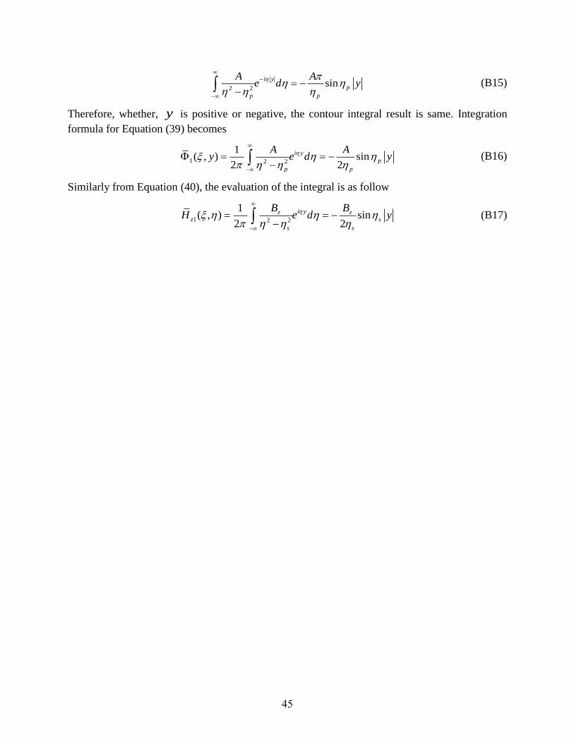
45
2 2
sini y
p
p p
A Ae d y
(B15)
Therefore, whether, y is positive or negative, the contour integral result is same. Integration
formula for Equation (39) becomes
1 2 2
1( , ) sin
2 2
i y
p
p p
A Ay e d y
(B16)
Similarly from Equation (40), the evaluation of the integral is as follow
1 2 2
1( , ) sin
2 2
i yz zz s
s s
B BH e d y
(B17)

46
APPENDIX C
INVERSE FOURIER TRANSFORM IN X- DIRECTION
The integrant in Equation (68) is singular at the roots of SD and AD , i.e.,
0SD (C1)
0AD (C2)
Equations (C1) and (C2) are the Rayleigh-Lamb equations for symmetric and anti-symmetric
modes.
The evaluation of integral in Equation (68) can be done by residue theorem using a close contour
as shown in Figure C1. The positive roots correspond to forward propagating waves. To satisfy
the radiation boundary condition at x , that is no incoming waves from infinity, the negative
real poles are avoided in the contour ( 0)x .
The integration of Equation (66) can be written as the sum of the residues,
1
( ) ( )1( ) ( )
2 ( ) ( )
12 Res( )
2k
i x i xS AS A
S A
k
N NI P e d P e d
D D
i
(C3)
For the poles k , Equation (C3) becomes
1 Res( )k
kI i
(C4)
Figure C1 Close contour for evaluating the inverse Fourier transform by residue theorem for (a) 0x (b) 0x

47
From residue theorem, if ( )
( )( )
N zf z
D z and z a is a simple pole then
( )Res( ) , where ( )
( )z a
N a dDa D a
D a dz
. Applying residue theorem to obtain the integration of
Equation (C3) we get
1
0 0
( )( )( ) ( )
( ) ( )
As AS j jj
j
AS jji xAi xjSS A
j jS AS Aj js j A
INN
i P e P eD D
(C5)
The summation of Equation (C5) is taken over the symmetric and anti-symmetric positive real
wavenumbers j
S and j
A . At given frequency , there are 0,1,2,...., Sj j symmetric Lamb
wave modes and 0,1,2,...., Aj j anti-symmetric Lamb wave modes.
Using Euler formula in Equation (69) and obtain
2
1cos cos sin
2 2p
AI d x i x d
(C6)
By using even and odd function property of the integrant, Equation (C6) becomes
2
0
cos cos2
p
AI d xd
(C7)
2
2
2
0
cos cos2
p
AI d c xd
(C8)
Apply integration by parts to Equation (C8)
2 2cos ; cos ; p
duu d c v x uvd u vd vd d
d
(C9)
After integrating by parts using Equation (C9), Equation (C8) becomes
22
22
20
sin
sin2
p
p
d cA d
I xdx
c
(C10)
The integration of Equation (C10) is to be evaluated with the aid of ref [53], pp 35 (23) for
12 and using 1
2
2( )J sin( )x x i.e.,
1 1
2 2 2 22 22 1Y
4p p
AI c d x d c x d
(C11)
Here 1Y is the Bessel function of second kind of order 1.
Upon rearrangement of Equation (70)

48
2 2
32 2
1sin
2 2
i xzs
s
BI c d e d
c
(C12)
The integration of Equation (C12) is to be evaluated by contour integration with brunch cut. The
poles are sc . The closed path for contour integral is shown in Figure C2 [51]. The
corresponding arguments are listed in Table 1.
Table 2 Arguments for inverse Fourier transform
Line 2 2
sc
DE
+ i
2 2
sc
EF
+
2 2
sc
GH
+ 2 2
sc
HI
+ i
2 2
sc
Figure C2 Close contour for evaluating the inverse Fourier transform for 0x
After applying the arguments as shown in Table 1 the Equation (C12) becomes

49
2 2
32 2
2 22 2/
2 22 20 0
2 2/
2 20
1sin
2 2
sin sin1 1cos
sinsin
s
s
i xzs
s
c
z s z sx
s s
c
z s
s
BI c d e d
c
B d c B d ce d x d
c c
B d cix d
c
(C13)
Equation (C13) turns into three integrals. Let assume that
3 31 32 33I I I I (C14)
Where,
2 2
312 2
0
sin s xz
s
d cBI e d
c
(C15)
2 2/
322 2
0
sincos
sc
sz
s
d cBI x d
c
(C16)
2 2/
332 2
0
sinsin
sc
sz
s
d ciBI x d
c
(C17)
Equation (C15) accepts imaginary wave number. The imaginary wavenumber correspond to non-
propagating evanescent waves and will not be considered here.
The integrant in Equation (C16) can be evaluated by with the aid of ref [53], [54], i.e.,
1 1
2 2 2 22 232 0( ) J ( )
2
z
S S
BI x x d x d
c c
(C18)
Here 0J is the Bessel function of first kind of order 0.
Equation (C17) is to be determined from ref [53], pp. 35 (23), by putting 12 and using the
identity of Bessel function, 12
J ( ) 2 sinx x x i.e.,
1 1
2 2 2 22 233 1( ) ( ) Y ( )
2
z
S S
iBI x x d x d
c c
(C19)
Using Equations (67), (C5), (C11), (C18), (C19) the total displacement becomes

50
1 12 2 2 22 2
1
1 1
2 2 2 22 20
0 0
Y4
( ) J ( )2
( )( )( ) ( )
( ) ( )
As AS j jj
j
y
P P
z
S S
AS jji xAi xjSS A
j jS AS Aj js j A
u
Ad x d x d
c c
Bx x d x d
c c
i
NNi P e P e
D D
1 1
2 2 2 22 21( ) ( ) Y ( )( )
2
z
S S
Bx x d x d
c c
(C20)