fukino project discussion paper series

Fukino Project

Discussion Paper Series

No.016

Inter-Industry Wage Differentials:

An Increasingly Important Contributor to Urban China Income Inequality

Zhao Chen

China Center for Economic Studies, and Center for Industry Development, Fudan University

Ming Lu

School of Economics, Fudan University and Zhejiang University

Guanghua Wan

Asian Development Bank

December 2009

Hitotsubashi University Research Project of Policies for East Asia

Hitotsubashi University

2-1 Naka, Kunitachi, Tokyo, 186-8601 Japan

Inter-Industry Wage Differentials:

An Increasingly Important Contributor to Urban China Income Inequality

Zhao Chen, Ming Lu and Guanghua Wan*

Abstract: How significantly inter-industry wage differentials contribute to rising

income inequality is an essential policy issue for transitional economies. Using

regression-based inequality decomposition, this paper finds that inter-industrial wage

differentials contributed increasingly to income inequality in urban China through

1988, 1995, and 2002, mainly due to rapid income growth in monopolistic industries.

Factors such as region, education, ownership, occupation, and holding a second job

also contribute increasingly to income inequality, while being employed the whole

year and age have decreasing contributions. If China seeks to reduce urban income

inequality, removing entry barriers in the labor market and breaking monopoly power

in the goods market are essential policy prescriptions.

Keywords: Inter-industry wage differentials; Income inequality; Regression-based

decomposition

1. Introduction

As one of the fastest-growing countries in the world, China needs to face the challenge of

widening income inequality. Although many researchers have focused on interregional and

urban-rural income inequality, as well as individual-level inequality, few have studied the rising

inter-industrial wage differential. In this paper, we use regression-based inequality decomposition

to sort various factors that influence income inequality according to their importance. Our results

suggest priorities for policies that reduce income inequality. We find that inter-industry wage

differentials have contributed increasingly to Chinese urban inequality during 1988, 1995, and

* Zhao Chen: China Center for Economic Studies, and Center for Industry Development, Fudan University,

Shanghai, China, Email: [email protected]; Ming Lu: School of Economics, Fudan University and

Zhejiang University, Email: [email protected]. Guanghua Wan: Asian Development Bank, Email: [email protected].

Financial support from the National Social Science Foundation (08BJL008), MOE Project of Key Research

Institute of Humanities and Social Sciences at Universities, the Shanghai Leading Academic Discipline Project

(B101) are greatly appreciated. We thank seminar participants at UNU/WIDER for their useful comments. The

1

2002, mainly due to the high rapid income growth in monopolistic industries. This finding is

particularly important for understanding the direction of the Chinese market economy. Combating

monopoly power is essential for China’s next step in reforms to build a competitive and efficient

market, as well as to narrow income inequality and achieve social justice.

Worldwide research into inter-industry wage differentials has continued for more than 20

years. Research in China indicates that higher salaries in monopolistic industries are regarded as

“unfair” rather than “an inequality” justified by factors such as workers’ higher education or job

skills. Although many argue that China should pay greater attention to rising inequality among

industries, there has been no measure of the magnitude of the industry factor’s contribution to

income inequality or to the trend of this magnitude. Therefore, we do not know how well

competition-inducing policies to combat a monopoly can narrow income inequality and whether

China’s current marketization reform can reduce inter-industry wage differentials.

In a well-developed market system, full competition in the labor market can assure

equalization of income among different industries. In other words, as long as specific industries

impose no entry barriers on the labor market, inter-industry income differentials would be

determined only by the individual characteristics rather than by the industries where people work.

Therefore, in the process of marketization toward full competition, inter-industry factors should

have decreasing contribution to income inequality, which would indicate that China is becoming a

market economy with fair competition. However, we obtained the opposite finding. Although there

is increasing competition in the market, the extent of competition varies across industries. The

state-owned monopolistic industries have been minimally affected by reform. The legal system for

antitrust activities is by no means effective, and it was especially ineffective before August 2008,

when China’s first Antitrust Law took effect. In the financial sector the four major state-owned

banks were commercialized according to the Law of Commercial Banks in 1995, but it is hard to

say as the banking sector became highly competitive. For instance, in late 1990s Urban Credit

Cooperatives in cities were merged into some Urban Commercial Banks, thus increasing market

power of the existing banks. The effect of competition policy in the telecommunication sector is

also unsatisfactory. In 2002, China Netcom① was separated from China Telecom and was

supposed to compete with the new China Telecom. At that time, China Netcom’s market was

northern China and China Telecom’s was in the south. However, in February 2007 China Netcom

content of this article is the sole responsibility of the authors.

2

and China Telecom agreed not to enter each other’s markets. These instances imply that China’s

gradual reform is not necessarily leading to a market economy with full competition. Without

narrowing inter-industry wage differentials, the current marketization reform in China may lead to

an unfair market economy. The finding also indicates that controlling inter-industry wage

differentials would be a conducive and important policy to reduce Chinese urban inequality.

The remainder of this paper is organized as follows. Section 2 briefly reviews literature related

to inter-industrial inequality. Section 3 describes the background and facts of the Chinese labor

market reform and inter-industry inequality. Section 4 reports data and income equations. Section

5 presents results of the regression-based income inequality decomposition. The final section

concludes and discusses policies based on this paper.

2. What do we know about inter-industry inequality? A literature review

Since the mid-1980s, it has generally been accepted that inter-industry wage differentials are

widely evident. The following research has inquired mainly into the causes of inter-industry wage

differentials. The basic conclusion is that in the income equation using OLS estimation the omitted

variables (such as ability) might be correlated with an industry variable, thereby leading to an

over-estimated inter-industry wage differential. In recent research using siblings’ data to control

unobserved fixed effects, 11% to 24% of inter-industry wage differentials are correlated to

unobserved factors co-owned by brothers in north Europe, while in the U.S., this percentage is up

to 50%. After controlling those fixed effects by differencing siblings data, the range of

inter-industry wage differentials for the U.S. and northern Europe are close (Björklund, et al.,

2004). Haisken-DeNew and Schmidt (1999) used panel data in Germany and the U.S. to control

fixed effects. They found that personal heterogeneity can explain almost a half of inter-industry

wage differentials. Even by controlling the standard human capital, job characteristic, job identity,

and geographical factors, inter-industry wage differentials in Germany and the U.S. are still large

and similar. Pinheiro and Ramos’s (1994) research in Brazil discovered a huge inter-industry wage

differential in the labor market. Even after controlling for differences in workers’ productivity and

occupation characteristics, the inter-industry wage differential remains and cannot be explained by

quality of work, worker’s heterogeneity, discrimination, short-term excess demand in specific

① In 2008, China Netcom was merged into China Unicom.

3

sectors, or fluctuations in macroeconomic status and policies.

What other factors influence the inter-industry wage differential? Theoretically, reduced

competition in the goods market and in the labor market are important factors explaining the

inter-industry wage differential. Monopoly power enables enterprises to obtain monopoly profits,

which allow employers to pay higher wages. Non-competitiveness of labor markets is another

condition contributing to inter-industry wage differentials. If there are no entry barriers in the

labor market, employers need not pay wages above the market-clearing equilibrium. Krueger and

Summers (1988) found that inter-industry wage differentials exist even after controlling

measurable and immeasurable labor quality, working conditions, excess welfare, short-term

demand shock, unionization threats, bargaining power of labor union, an enterprise’s scale, etc.

They also found that higher wages were related to lower labor-turnover in an industry, which

demonstrates that high-wage industries obtain some rent from non-competitiveness. Katz and

Summers (1989) also believed workers receive rents in high-wage industries. These rents might

appear because some industries are willing to pay above-market wages to achieve higher

productivity. This mechanism is called “an efficiency wage.” Evidence provided by Chen and Edin

(2006) supports the efficiency wage hypothesis. Similarly, Gittleman and Wolff (1993) found that

inter-industry wage differentials are positively correlated to an industry’s productivity growth rate,

output growth rate, capital intensity, and export orientation. Arbache (2001) used comparable and

measurable productivity characteristics to explain wage differentials. He finds no evidence to

support the compensatory wage, but he does find the existence of an efficient wage mechanism in

manufacturing industries.

The inter-industry wage differential is widening in transitional economies like China and

Russia and is stable in developed economies. In China, Shi (2007) reported the trend of widening

inter-industry wage differentials. The ranking of industry wages changed dramatically in the 1980s

and stabilized after the mid-1990s. In Russia, the relative change of the inter-industry average

wage was the main reason for the widening income gap (Lukyanova, 2006). In other countries,

empirical research shows that inter-industry wage differentials in the U.S. widen after the 1970s,

mainly because of the widening wage differential between the primary and secondary sectors

(Davidson and Reich, 1988). Using panel data from the 14 OECD countries for the period 1970-85,

Gittleman and Wolff (1993) found that rankings of inter-industry wages were stable. They found

4

that inter-industry wage differentials in the U.S. were generally widening, but the trend in other

countries is unclear. Haisken-DeNew and Schmidt (1999) found that inter-industry wage

differentials for Germany and the U.S. were stable during the 13 years they studied. Between 1984

and 1998, a period of dramatic structural change in Brazil, the wage structure there was relatively

stable (Arbache, 2001; Arbache, Dickerson, and Green, 2004). Using historical data for the U.S.,

Krueger and Summers (1987) found that the correlation coefficient of relative wages for nine main

industries was 0.62 during the period 1900–1984, while correlation for the years between 1970 and

1984 was 0.91.

Among the literature we have surveyed there is little research using decomposition methods to

determine various factors’ contribution (including an industry factor) to income inequality and the

trend of the contribution. Pinheiro and Ramos (1994) used the decomposition method to study

Brazil’s data. After controlling for other variables, they found that the contribution of labor market

segmentation to income inequality is between 7% and 11%. In this paper, we use Chinese data to

show the contribution of inter-industry wage differentials to income inequality and to document

how the contribution changes over time. We will provide new empirical evidence of inter-industry

wage differentials in China as it undergoes economic transition. Knight and Song (2003)

decomposed Chinese urban residents’ income inequality, but they did not consider the contribution

of inter-industry inequality. Gustafsson and Li (2001) decomposed income inequality according to

income sources, but the method they use cannot identify the contribution of basic determinants of

income to income inequality. To our knowledge, only the recent paper by Deng and Li (2009)

decomposed urban inequality and derived the contributions of each factor over time. Their

decomposition results indicate that the effects of gender and membership in the Communist Party

of China on earnings inequality have changed little. While work experience had a reduced effect

on earnings inequality, the effects of education and occupation have increased. The contributions

of ownership status and industry to earnings inequality have increased. Regional effects have been

the largest recent contributor to earnings inequality. Unlike the work of Deng and Li (2009), where

the industry factor is a minor result in their study, our focus is how inter-industry wage

differentials contribute to income inequality and how the contribution changes over time in China.

We also will provide evidence indicating that relatively rising earnings in several industries

dominated by state-owned-enterprises mainly explains why the contribution of industry to

5

inequality increases over time. In model specification, our income-generating function also differs

slightly from Deng and Li (2009). Our approach includes more explanatory variables, such as

dummies for holding a second job and being employed the whole year, to capture the structural

change of the labor market and to alleviate potential missing-variable-bias.

3. Chinese labor market reform and inter-industry inequality: background and

fact

Among components of overall income inequality in china, urban residents’ income inequality is

becoming increasingly significant. Income inequality of rural and urban residents and overall

income disparity are widening. Urban residents’ inequality is smaller than rural residents’, but the

difference between these two inequalities is decreasing. In 2001, the rural Gini coefficient was

36.48, the urban Gini coefficient was 32.32, and the national overall Gini coefficient was 44.73

(Ravallion and Chen, 2007). Other research analyzing data of 1988, 1995, and 2002 found income

inequality widening rapidly between 1998 and 1995, but it changed little from 1995 to 2002. The

overall Gini coefficient changed from 46.9 to 46.8, while the urban Gini coefficient declined from

33.9 to 32.2. In fact, the stable trend of overall income inequality is mainly due to income

convergence in eastern provinces (Gustafsson, Li, and Sicular, 2008).

Some factors in the process of urban reform increase income inequality. Before reform and

opening-up, all urban Chinese workers were employed by state-owned or collective-owned

enterprises; and all their income came from wages, which were solely decided by the planning

system. Except for factors such as position and age, the value system of “equal pay for equal

work” controlled returns on other factors, such as education and gender, at a low level. For the

determination of wages, working age was more important than productivity (education)

(Gustafsson et al., 2001). Since wage levels were set by the labor administration department,

generally speaking, the profit differential across industries and enterprises did not produce a

difference in wages for employees.

Since the reform and opening-up, the greatest change in the determination of wage and

income is the increase of education returns and the widening inter-industry wage differential.

Marketization reform raised the return on human capital, which was previously distorted under the

planning system. Much empirical research has found that along with China’s reform and

6

opening-up, the returns to education rose continuously (to name a few: Zhang et al., 2005; Li and

Heckman, 2004; Li and Ding, 2003). Education has an increasing influence on income inequality

(Gustafsson, Li and Sicular, 2008). For example, according to empirical evidence from Shanghai,

the commercial center of China, education has the greatest contribution to income inequality (Tian

and Lu, 2007).

Let us look at the widening inter-industry wage differentials, Figure 1 shows wage

inequality among more than 10 industries since 1978 according to two indexes. The simplest index

is the ratio of the highest to the lowest industry average wage. From 1978 to 1997, this index rose

from 1.66 to 2.26, and then rapidly rose to 4.75 until 2006. The other index is the Gini coefficient

of all industries’ wages. We take all employees from the same industry as a group earning the same

wage and use the number of employees from this industry as the size of the group to calculate the

Gini coefficient. The result calculated in this way also shows a rising trend. The Gini coefficient

was 0.05 in 1978, 0.1 in 1997, and rose rapidly to 0.19 until 2006①.

0

0.05

0.1

0.15

0.2

0.25

1978

1980

1982

1984

1986

1988

1990

1992

1994

1996

1998

2000

2002

2004

2006 Year

Gini

0

1

2

3

4

5

6Wage gap

Gini

Wage gap

Fig. 1: China’s inter-industry wage differential (1978–2006)

Data source: China Statistical Yearbook (various years), Chinese Statistics Press, and the

authors’ calculation.

① Because of neglecting wage differential within the same industry, the Gini coefficient calculated here is smaller than the real value of Gini coefficient for all employees.

7

We mark 1997 as the dividing line to compare the change of inter-industry wage differentials

because 1996 was the watershed year for labor market reform. Before 1996, reform in the labor

market was relatively moderate. The obvious adjustment at that time was that wages had dropped

continuously as a share of total income (Lu and Jiang, 2008). The decentralization reform in the

1980s gave enterprises more power in deciding wages and bonuses. Enterprise revenue

differentials were reflected in the income inequality. Incentive scheme reform promoted enterprise

efficiency significantly (Groves et al., 1994). However, at the same time, it made the revenue

differential among industries and enterprises contribute to the differential in employees’ wages.

Using survey data of state-owned enterprise in 1981 and 1987, Meng and Kidd (1997) found that

the inter-industry wage differentials among Chinese state-owned enterprises had become more

remarkable since 1987. They believe the main reason is that after the reform of the employment

system, enterprises implemented profit-linked bonuses (Meng and Kidd, 1997). In 1996, with the

re-employment service center as an intermediary, Shanghai began to lay off redundant workers in

state-owned enterprises. After that, labor market reform accelerated, employment structure

adjusted rapidly, and the labor force participation rate decreased sharply (Lu and Jiang, 2008). The

widening of urban income inequality after 1996 resulted from labor market restructuring (Meng,

Gregory, and Wang，2005). It is noteworthy that labor market reform after 1996 began in

money-losing enterprises, which were mostly in the competitive sector. Policies at that time

allowed state-owned enterprises with two years of losses to cut redundant employment through

lay-offs and repositioning. However, competition in the labor market exists marginally. Monopoly

sectors such as public utilities, post and communication, and finance were less influenced by the

labor market competition. According to Figure 2, as a whole, employment in sectors with lower

wages decreased more in 1996–1998, while employment increased in higher-wage sectors①. This

phenomenon is similar to the lower employment turnover in higher-wage industries in the U.S.

(Krueger and Summers, 1988). Moreover, during the 1980s, although the labor market became

more flexible, the labor flow both between urban and rural areas and among cities was not

remarkable (Davis, 1992). After the mid-1990s, large scale rural-urban migrants intensified

competition in the urban labor market, but this marginal increase in competition was concentrated

① The outlier in the left of Figure 2 is “other industry,” which has higher employment increasing rate. If omitting this point, wage and employment change still have positive relationship and the fitting degree rises to 0.34.

8

only in industries with fewer labor market entry barriers. The influence of increasing competition

is different for various industries; that is the main reason for the widening inter-industry wage

differentials.

In the following two sections, we will see the contribution of the inter-industry wage

differential to income inequality and its changes over time. In addition, we will see that the

increasing contribution of the inter-industry wage differential to inequality results primarily from

several state-owned monopolistic industries.

Fig. 2: Income and employment change in 1996–98

4. Data and income equation

Data used in our research are from the Chinese Household Income Project Survey (CHIPS)

conducted by the Chinese Academy of Social Science and the National Bureau of Statistics.

CHIPS data are collected randomly following a strict sampling process, are nationally

representative, and are widely used in research. In our data, the 1988 urban survey covers 10

provinces including Beijing, Shanxi, Liaoning, Jiangsu, Anhui, Henan, Hubei, Guangdong,

Yunnan, and Gansu. The 1995 data include one additional province, Sichuan. The 2002 data cover

the same provinces as 1995 plus the new municipality, Chongqing.

Our research has two steps. First, we need to estimate a semi-log income-generating

equation, and then we decompose income inequality based on this equation. The

income-generating equation we estimate can be written as: In Wit = βt’Xit + εit, where W is the

individual’s annual earnings (including wage, bonus, price subsidy, income in kind, and secondary

96-97 changing rate of employment

y = 1E-05x - 0.0665

R 2 = 0.0805

-0.1

-0.05

0

0.05

0.1

0.15

0.2

0.25

0 2000 4000 6000 8000 10000

wage in 1996

97-98changing rate of employment

y = 4E-05x - 0.3748R 2 = 0.3581

-0.35

-0.3

-0.25

-0.2

-0.15

-0.1

-0.05

0

0.05

0.1

0 2000 4000 6000 8000 10000 12000wage in 1997

9

job income), i denotes the individual, t denotes year (t = 1988, 1995, and 2002), and X is a vector

of the explanatory variables. Following existing literature, explanatory variables for income

include age and its square, years of schooling, dummies for holding a second job, being employed

the whole year, gender, party membership, minority groups, ownership types, and occupation

classifications. We also controlled the city dummy. βt is a vector of parameters to be estimated. In

order to make the income data comparable across region and time, we need to deflate income data.

Brandt and Holz (2006) provided the interregional price index in 1990, which indicates the

purchasing power of the RMB among different regions. Using this interregional price index in

1990 and the provincial level urban consumer price index, we obtain the price deflator for 1988,

1995, and 2002. By doing so, the deflated income becomes comparable not only across time but

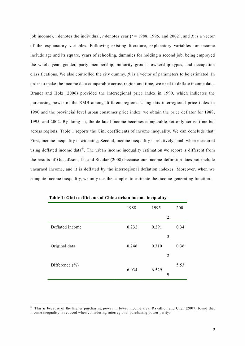
across regions. Table 1 reports the Gini coefficients of income inequality. We can conclude that:

First, income inequality is widening; Second, income inequality is relatively small when measured

using deflated income data①. The urban income inequality estimation we report is different from

the results of Gustafsson, Li, and Sicular (2008) because our income definition does not include

unearned income, and it is deflated by the interregional deflation indexes. Moreover, when we

compute income inequality, we only use the samples to estimate the income-generating function.

Table 1: Gini coefficients of China urban income inequality

1988 1995 200

2

Deflated income 0.232 0.291 0.34

3

Original data 0.246 0.310 0.36

2

Difference (%) 6.034 6.529

5.53

9

① This is because of the higher purchasing power in lower income area. Ravallion and Chen (2007) found that income inequality is reduced when considering interregional purchasing power parity.

10

Table 2: Income-generating functions of different years

1988 1995 2002

Socio- economic characteristics

Second job (yes = 1) 0.058** 0.362*** 0.150***

Being employed the whole year (yes = 1) 0.643*** 0.455*** 0.444***

Gender (male = 1) 0.079*** 0.152*** 0.122***

Age 0.084*** 0.160*** 0.055***

Age square −0.001*** −0.002*** −0.0006***

Minority group (yes = 1) 0.024 −0.013 −0.036

Industry

Farm, forest, husbandry and fishery 0.014 0.039 0.011

Mining and exploration industry 0.065*** 0.020 −0.0007

Geological prospecting, irrigation administration −0.028 0.116

Electricity, gas and water supply facilities, architecture 0.317***

Construction 0.001 −0.051 0.070**

Transportation, storage, post office and communication 0.001 0.047* 0.163***

Wholesale, retail and food services −0.004 −0.028 −0.027

Real-estate −0.069*** −0.022 0.203***

Social services −0.186*** −0.091***

Health, sports and social welfare 0.016 0.036 0.050

Education, culture and arts, mass media and

entertainment

0.0001 0.068*** 0.067

Scientific research and professional services −0.017 0.064 0.110

Finance and insurance 0.003 0.196*** 0.210***

Government agents, party organisations and social

groups

−0.038*** 0.014 0.084

Other industries −0.018 −0.259*** 0.047

City dummy yes yes yes

Constant 6.529*** 4.861*** 7.088***

11

Number of Observation 17568 10933 6121

Adj-R2 0.473 0.336 0.383

Note: (1) The classification of industries is consistent with CHIPS questionnaire, which is a little different

from the classification of China Statistical Yearbook. (2)Control variables include dummies for party membership,

education level, ownership type, occupation type, city dummies, etc. Because of space limitations, we do not

report coefficients of party membership and education level. (3) *, **, and *** denote significance at 1%、5% and

10% level, respectively. To save space, standard error is not reported.

5. Regression-based decomposition of income inequality

In this section, we analyze how different variables contribute to income inequality using a

regression-based decomposition framework developed by Shorrocks (1999), focusing on the

contribution of industry variables and its change across time. The idea of this method is to

calculate a sample average value of an argument (such as X) in the income determination function,

then substitute X by its average, predict income data, and compute the inequality index of this

predicted income. This new inequality index does not include the influence of “X.” X’s

contribution to income inequality is measured by the difference between this new index, and the

income inequality computed before X is replaced by its average. Above is a brief introduction of

the decomposition method in this paper. A more-detailed introduction can be found in Wan (2004)

or Wan and Zhou (2005).

Because we choose a semi-log model in the income-generating function, we will get

erroneous results if we use the logarithm of income as the dependent variable to do decomposition;

therefore, we take the exponent while writing the income-generating equation for decomposition.

0 1 1 2 2ˆ ˆ ˆ ˆ ˆex p ( ) ex p ( ) ex p ( )k ky a a X a X a X u

In the above equation 0ˆexp( )a is a scalar. When we compute indices of income inequality, the

scalar can be omitted from the equation without influencing the results (Wan, 2002). Considering

the influence of residual u , we employ a popular method that can be used by any index to

measure inequality. We take the difference between the inequality index of original income y

and the inequality index when assuming u ＝ 0 as residual u ’s contribution to the actual

income inequality. In the ideal status, the residual is 0, and total income inequality can be

12

explained 100% by variables in the income-generating function that fits the data perfectly.

Generally, however, the residual is seldom 0, so the analysis of residual influence is necessary. In

Table 3, we adopt the ratio of the residual’s contribution to total income inequality as the

proportion explained by the residual. The rest reflects the income inequality contributed by the

explanatory variables in the model (Wan，2002). According to this principle, our model can

explain approximately 81%, 78%, and 67%, respectively, of total income inequality.

Table 3: China urban income Gini and the proportion explained

1988 1995 2002

Gini coefficient computed by original income data 0.232 0.291 0.343

Gini coefficient computed by predicted income data 0.189 0.227 0.228

Proportion explained by residual (%) 18.534 22.129 33.448

Proportion explained by model (%) 81.466 77.871 66.552

Because there is some difference in industrial classification in these three years, we cannot

directly compare income inequality decomposition results of different years. So we first focus on

the decomposition results for 2002. Because the regression-based decomposition method we use

can be applied to different inequality indices, we use data in 2002 to decompose four different

indices of income inequality. Table 4 reveals an issue that arises when using different indexes:

although the factors employed in each index are the same, their contributions to income inequality

differ in each index. This is because each index applies a different weighting to income groups

from the poorest to the richest. Notwithstanding this variation among indexes, however, each

factor’s rank in contributing to income inequality does not change.

The most important contributor to income inequality is the city dummy variable, which

represents different regional factors such as geography, institution and culture, etc. This variable’s

contribution to income inequality ranges from 31.984% to 37.02%. The great contribution of

region dummies to urban residents’ income inequality reflects the persistent barriers to Chinese

labor mobility that are noted by Davis (1992). Based on Gini decomposition results, the second

level contains four factors: occupation, ownership, education, and industry, each contributing

13

approximately 10% to income inequality. Contribution factors at the third level are age, being

employed the whole year, and gender, which have contributed between 5% and 6.8%.

Contributions of holding a second job and party membership are 3.321% and 3.982%, respectively.

The contribution of the minority group dummy is trivial. In fact, in our income-generating

function, membership in a minority group is also an insignificant factor, which means that China

does not have discrimination against minority groups.

Table 4: Decomposition of income inequality for 2002 (industry is of original category)

Gi

ni

% GE(0

)

% GE (1) % CV %

Second job 0.009 3.982 0.002 2.749 0.002 2.787 0.005 2.811

Being employed

the whole year

0.015 6.613 0.008 9.253 0.007 7.926 0.012 6.828

Gender 0.011 5.004 0.004 4.287 0.004 4.203 0.007 4.112

Age and its

square

0.016 6.803 0.005 6.151 0.005 5.595 0.009 5.034

Party

membership

0.008 3.321 0.003 3.060 0.003 3.104 0.006 3.176

Minority group 0.000 0.074 0.000 −0.019 0.000 −0.016 0.000 −0.017

Education 0.024 10.373 0.009 10.118 0.009 10.656 0.020 11.296

Ownership 0.024 10.630 0.008 9.753 0.008 9.665 0.017 9.547

Occupation 0.025 11.148 0.009 10.910 0.009 10.799 0.019 10.771

Industry 0.023 10.067 0.008 9.186 0.008 9.332 0.017 9.422

City dummy 0.073 31.984 0.029 34.551 0.030 35.948 0.067 37.020

total 0.228 100.000 0.085 100.000 0.084 100.000 0.180 100.000

What importance does the variable “Industry” have in contributing to income inequality?

If we decompose income inequality and estimate the income equation entirely according to

industrial categories based on original data, this factor contributes increasingly to income

14

inequality, from 1.03% in 1988 to 3.02% in 1995, then 10.07% in 2002. Its rising contribution

from 1995 to 2002 is dramatic. To accommodate for the official re-classification of industries in

three different years, we combine some industries to make industry dummies comparable across

time. For instance, we combined the exploration and mining industries for 1988 and 2002. Also for

these two years, we combined the category “social service” with “public health, sports, and social

welfare,” which also merges the categories “electric, gas, and water suppliers” for 2002. After

doing so, we establish 13 industries, including “other,” which fall into categories that are

comparable across several years.

In Table 5, we report 11 factors contributing to income inequality in all three years. It

shows the following trends: (1) The industry factor’s contribution to income inequality grows. For

2002, we combine the category “electricity, gas, and water production and supply” that has higher

income, with “social services” that has lower income, and with “public health, sports, and social

welfare,” which has insignificantly higher income compared to manufacturing. Therefore, the

contribution of industrial category to income inequality is lower, but it still produces a greater

contribution to income inequality than in 1995. (2) The location factor, represented by the urban

dummy, has a growing contribution to income inequality. In 1988, the location factor contributed

14% to income inequality, ranking in first place, but its contribution had increased to 30% in 1995,

becoming the most important contributor to income inequality. It could explain one-third of total

income inequality in 2002. The regional variable’s rising contribution to income inequality can be

explained by barriers to labor-flow for low-skilled labors among cities, but relatively free mobility

for high-skilled laborers. (3) Education has an apparently increasing contribution to income

inequality. Now that reform permits higher wages for education and training, its increasing

contribution is not surprising. (4) Ownership and occupation also contribute increasingly to

income inequality, although occupation’s contribution increases faster. This may be explained by

intense restructuring in forms of ownership and occupation. (5) Being employed the whole year

has an apparently decreasing contribution to income inequality. For 1998, this factor explains up

to one-third of income inequality, which was caused by a large number of surplus workers in

enterprises. In our 1988 sample, 9.47% of people were not employed the whole year. But in 1995,

this factor’s contribution had decreased dramatically to 7.4%. In that year, only 7.86% of people

were not employed the whole year. In 2002, this factor’s contribution dropped to 6.7%. (6) Age

15

also has an understandably decreasing contribution. Older workers were paid more under

traditional working system, so it had a great contribution from 1988 to 1995. But in 2002, after

rapid labor market reform beginning in 1996, age’s importance has dropped, while other factors of

productivity have influenced income more. (7) Holding a second job has an apparently increasing

contribution to income inequality. In 1995 its contribution to income inequality was more than

three times greater than in 1988, and in 2002 its contribution was 7.5 times greater than in 1995.

Table 5: Income inequality (Gini) decomposition (industries combined)

1988 1995 2002

Gini % Gini % Gini %

Second job 0.000 0.147 0.001 0.558 0.009 4.178

Being employed the

whole year

0.061 32.501 0.017 7.422 0.015 6.733

Gender 0.009 4.603 0.014 6.245 0.012 5.363

Age (and its square) 0.053 27.868 0.051 22.378 0.016 7.116

Party membership 0.006 3.252 0.010 4.383 0.007 3.219

Minority group 0.000 0.114 0.000 0.049 0.000 0.081

Education 0.004 1.939 0.019 8.410 0.025 11.122

Ownership 0.018 9.475 0.023 9.967 0.028 12.250

Occupation 0.011 5.641 0.018 7.735 0.028 12.623

Industry 0.001 0.406 0.007 3.019 0.011 5.086

City dummy 0.027 14.055 0.068 29.834 0.072 32.229

Total 0.189 100.000 0.227 100.000 0.225 100.000

According to regression results of Table 2, the coefficients of two

industries—“transportation, storage, post office, and communication” and “finance and

insurance”—change from insignificant to increasingly significant. Coefficients of these two

industry categories also increase. We suspect that these two industries increase the industry

variable’s contribution to income inequality rapidly. Galbraith, et al., (2004) note that in Russia

16

and China industries having the strongest monopoly power gained relatively during economic

restructuring. In both countries, the financial sector gained the most, while the agricultural sector

lost the most. Therefore, in the following step we exclude these two industries, which have the

highest income. In conclusions presented in Table 6, the contribution of factors other than industry

changes little, but industry contribution has greatly decreased. For 2002, industry leaves the

second layer of factors in terms of their contribution. Its contribution to income inequality ranks

9th of 11 factors and dropped by 0.13% from 1995 to 2002. Therefore, we can conclude that two

industries—“transportation, storage, post office and communication” and “finance and

insurance”—have become the important elements in widening urban residents’ income inequality,

while the income of these two industries is relatively rising. Due to data limitation, we lack more

detailed categories of industries. However, the two industries excluded from the analysis include

state-owned sub-industries with monopoly powers.

Table 6: Income inequality (Gini) decomposition (industries combined, and two highest

income industries excluded)

1988 1995 2002

Gini % Gini % Gini %

Second job 0.000 0.137 0.001 0.627 0.010 4.430

Being employed

the whole year

0.060 31.892 0.017 7.511 0.016 7.177

Gender 0.009 4.656 0.015 6.457 0.013 5.621

Age (and its

square)

0.052 27.634 0.048 21.367 0.015 6.868

Party membership 0.006 3.383 0.010 4.382 0.008 3.526

Minority group 0.000 0.136 0.000 0.091 0.000 0.173

Education 0.004 2.090 0.018 8.149 0.023 10.194

Ownership 0.018 9.570 0.023 10.230 0.028 12.695

Occupation 0.010 5.547 0.018 8.073 0.031 13.712

Industry 0.001 0.424 0.005 2.421 0.005 2.292

17

City dummy 0.027 14.529 0.070 30.691 0.074 33.313

Total 0.188 100.000 0.227 100.000 0.223 100.000

6. Conclusions and policy implications

This paper primarily explores inter-industry wage differentials by examining the contribution that

industry variables make to urban residents’ income inequality and how the contribution changes

over time. We find that, concerning the process of widening urban residents’ income inequality,

inter-industry wage differentials also expand. Among all factors that widen inequality in our model,

the importance of inter-industry wage differential is increasing. During the period 1995–2002, the

increasing contribution of inter-industry wage differential was mainly attributable to the

monopolistic industries of “transportation, storage, post office and communication” and “finance

and insurance.” This suggests that in the marketization process, some industries benefit more, and

more intense competition in the labor market does not affect every industry equally. In addition,

we found that region, education, ownership, occupation, and holding a second job also contribute

increasingly to income inequality, while the factors like age and being employed the whole year

have a decreasing contribution.

The main policy implication of this paper is clear: if China wants to control urban income

inequality, removing entry barriers in the labor market and breaking monopoly power in the goods

market are essential. China needs to build a fairly competitive market economy to control income

inequality. According to results of 2002, urban residents’ income inequality would decease

5%–10% if China could remove inter-industrial wage differentials. In fact, just removing several

industries’ unreasonably high wage can make the industrial factor much less important in urban

income inequality. Of course, in order to reduce urban income inequality, the policy for regional

and educational equality is also important. The high inter-regional income inequality reflects the

situation that workers cannot freely move across regions because of institutional barriers induced

by the household registration (Hukou) system. Therefore, the main policy for reducing regional

income inequality should be to eliminate barriers to labor mobility, not the present policy of

inter-regional financial transfers. Higher income through higher education is an inevitable result of

marketization reform. Therefore, reducing income inequality can better be achieved by equalizing

18

educational opportunity than by artificially suppressing wages of the educated. When

inter-regional labor migration becomes much freer in the future, income inequality will be greater,

despite increased returns on education, if rural residents receive insufficient education before they

enter the cities.

The empirical results of this paper suggest that many current market reforms are not

producing a more fair and competitive economy. Widening inter-industrial inequality reflects

injustice in the labor market, which induces increasingly greater dissatisfaction in the population.

Having provided evidence of inter-industrial inequality, we now need to provide evidence

explaining its causes. In a companion paper, we will present evidence indicating who receives the

opportunity to enter highly paid industries.

References：

Appleton, Simon, Lina Song and Qingjie Xia, 2005, “Has China Crossed the River? The Evolution

of Wage Structure in Urban China during Reform and Retrenchment,” Journal of Comparative

Economics, 33(4), 644–663.

Arbache, Jorge Saba, 2001, “Wage Differentials in Brazil: Theory and Evidence,” The Journal of

Development Studies, 38(2), 109–130.

Arbache, Jorge Saba, Andy Dickerson and Francis Green, 2004, “Assessing the Stability of the

Inter-industry Wage Structure isn the Face of Radical Economic Reforms,” Economics Letters,

83(2), 149–155.

Björklund, Anders, Bernt Bratsberg, Tor Eriksson, Markus Jäntti, and Oddbjörn Raaum, 2004,

“Inter-Industry Wage Differentials and Unobserved Ability: Siblings Evidence from Five

Countries,” IZA Discussion Paper Series, No. 1080.

Brandt, Loren and Carsten A. Holz, 2006, “Spatial Price Differences in China: Estimates and

Implications,” Economic Development and Cultural Change, 55(1), 43–86.

Chen, Paul and Per-Anders Edin, 2006, “Efficiency Wages and Industry Wage Differentials: A

Comparison across Methods of Pay,” The Review of Economics and Statistics, 84(4),

617–631.

19

Chen, Yi, Sylvie Démurger and Martin Fournier, 2005, “Earnings Differentials and Ownership

Structure in Chinese Enterprises, “Economic Development and Cultural Change, 53(4),

933–58.

Deng, Quheng and Shi Li, 2009, “What Lies behind Rising Earnings Inequality in Urban China?

Regression-based Decompositions,” CESifo Economic Studies, 55(3–4): 598–623.

Davidson, Carlos and Michael Reich, 1988, “Income Inequality: An Inter-Industry Analysis,”

Industrial Relations, 27(3), 263–286.

Davis, Deborah, 1992, “Job Mobility in Post-Mao Cities: Increases on the Margins,” China

Quarterly, 132, 1062–1085.

Dong, Xiao-Yuan, 2005, “Wage Inequality and Between-firm Wage Dispersion in the 1990s: A

Comparison of Rural and Urban Enterprises in China,” Journal of Comparative Economics,

33(4), 664–687.

Galbraith, James K., Ludmila Krytynskaia and Qifei Wang, 2004, “The Experience of Rising

Inequality in Russia and China during the Transition,” The European Journal of Comparative

Economics, 1(1), 87–106.

Gittleman, Maury and Edward N. Wolff, 1993, “International Comparisons of Inter-Industry Wage

Differentials,” Review of Income and Wealth, 39(3), 295–312.

Groves, Theodore, Yongmiao Hong, John McMillan and Barry Naughton, 1994, “Autonomy and

Incentives in Chinese State Enterprises,” Quarterly Journal of Economics, 109(1), 183–209.

Gustafsson, Björn and Shi Li, 2001, “The Anatomy of Rising Earnings Inequality in Urban

China,” Journal of Comparative Economics, 29(1), 118–135.

Gustafsson, Björn, Shi Li and Terry Sicular, 2008, Inequality and Public Policy in China,

NewYork: Cambridge University Press.

Gustafsson, Björn, Shi Li, Ludmila Nivorozhkina and Katarina Katz, 2001, “Rubles and Yuan:

Wage Functions for Urban Russia and China at the End of the 1980s,” Economic Development

and Cultural Change, 50(1), 1–17.

Haisken-DeNew, John P. and Christoph M. Schmidt, 1999, “Industry Wage Differentials Revisited:

A Longitudinal Comparison of Germany and USA (1984–1996),” IZA Discussion Paper

Series No.98.

Katz, L. F. and L. H. Summers, 1989, “Can Inter-Industry Wage Differentials Justify Strategic

20

Trade Policy,” in Feenstra, R. (ed.), Trade Policies for International Competitiveness,

University of Chicago Press, Chicago, 85–124.

Knight, John and Lina Song, 2003, “Increasing Urban Wage Inequality in China: Extent, Elements

and Evaluation,” Economics of Transition, 11(4), 597–619.

Krueger, Alan, and Lawrence Summers, 1988, “Efficiency Wages and the Inter-industry Wage

Structure,” Econometrica, 56(2), 259–293.

Li, Chunling, 2003, “Socio-Political Changes and Inequality of Educational Opportunity: Impact

of Family Background and Institutional Factor for the Education Acquiring (1940–2001),” (in

Chinese), Social Sciences in China, No. 3, 86–98.

Li, Shi and Sai Ding, 2003, “Long-term Change in Private Returns to Education in Urban China,”

(in Chinese), Social Sciences in China, No. 6, 58–72.

Li, Xuesong and James J. Heckman, 2004, “Heterogeneity, Selection Bias and the Return to

Education:A Empirical Analysis Based on Chinese Micro-Data,” (in Chinese), Economic

Research Journal, No. 4, 91–99.

Lukyanova, Anna, 2006, “Wage Inequality in Russia (1994–2003),” Moscow: Economics

Education and Research Consortium, Working Paper Series, No. 06/03.

Lu, Ming and Shiqing Jiang, 2008, “Labor Market Reform, Income Inequality and Economic

Growth in China,” China & World Economy, 16(6), 63-80.

Meng, Xin and Michael P. Kidd, 1997, “Labor Market Reform and the Changing Structure of Wage

Determination in China’s State Sector during the 1980s,” Journal of Comparative Economics,

25(3), 403–421.

Meng, Xin, Robert Gregory and Youjuan Wang, 2005, “Poverty, Inequality, and Growth in Urban

China, 1986–2000,” Journal of Comparative Economics, 33(4), 710–729.

Osburn, Jane, 2000, “Interindustry Wage Differentials: Patterns and Possible Sources,” Monthly

Labor Review, February, 34–46.

Pinheiro, Armando Castelar and Lauro Ramos, 1994, “Inter-Industry Wage Differentials and

Earnings Inequality in Brazil,” Estudios de Economia, 21, November, 79–111.

Ravallion, Martin and Shaohua Chen, 2007, “China's (Uneven) Progress against Poverty,” Journal

of Development Economics, 82(1), 1–42.

21

Shi, Xiancheng, 2007, “Monopoly Causes Inter-industry Wage Differentials,” China Economist,

November, 53–61.

Shorrocks, A., 1999, “Decomposition Procedures for Distributional Analysis: A Unified

Framework Based on the Shapley Value,” (unpublished manuscript), Department of Economics,

University of Essex.

Tian, Shichao and Ming Lu, 2007, “Contribution of Education to Within-City Income Inequality:

Evidence from Shanghai Household Data,” (in Chinese), South China Journal of Economics,

No. 5, 12–21.

Wan, Guanghua, 2002, “Regression-based Inequality Decomposition: Pitfalls and a Solution

Procedure,” World Institute for Development Economics Research discussion paper 2002/101,

Helsinki.

Wan, Guanghua, 2004, “Accounting for Income Inequality in Rural China: a Regression-based

Approach,” Journal of Comparative Economics, 32(2), 348–363.

Wan, Guanghua, Ming Lu and Zhao Chen, 2007, “Globalization and Regional Income Inequality:

Empirical Evidence from within China,” Review of Income and Wealth, 53(1), 35–59.

Wan, Guanghua and Zhangyue Zhou, 2005, “Income Inequality in Rural China: Regression-Based

Decomposition Using Household Data,” Review of Development Economics, 9(1), 107–120.

Zhang, Junsen, Yaohui Zhao, Albert Park, Xiaoqing Song, 2005, “Economic Returns to Schooling

in Urban China, 1988 to 2001,” Journal of Comparative Economics, 33(4), 730–752.

22

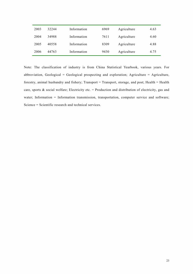
Appendix：The highest income and lowest income industry (1978–2006)

Year

Highest

Income

(yuan)

Highest Income

Industry

Lowest

Income

(yuan)

Lowest Income

Industry Ratio

1978 809 Geological 486 Agriculture 1.66

1979 885 Geological 503 Health etc. 1.76







1986 1543 Transport 1075 Agriculture 1.44

1987 1942 Transport 1162 Agriculture 1.67


1989 3288 Construction 1417 Agriculture 2.32

1990 2718 Mining 1541 Agriculture 1.76

1991 2942 Mining 1652 Agriculture 1.78

1992 3392 Electricity etc. 1828 Agriculture 1.86

1993 4320 Real estate 2042 Agriculture 2.12

1994 6712 Finance 2819 Agriculture 2.38






2000 13620 Science 5184 Agriculture 2.63

2001 16437 Science 5741 Agriculture 2.86


23

2003 32244 Information 6969 Agriculture 4.63




Note: The classification of industry is from China Statistical Yearbook, various years. For

abbreviation, Geological = Geological prospecting and exploration; Agriculture = Agriculture,

forestry, animal husbandry and fishery; Transport = Transport, storage, and post; Health = Health

care, sports & social welfare; Electricity etc. = Production and distribution of electricity, gas and

water; Information = Information transmission, transportation, computer service and software;

Science = Scientific research and technical services.

fukino project discussion paper series

Documents