from waste to fertilizer: evaluation of waste and waste

POLITECNICO DI MILANO

Scuola di Ingegneria Civile, Ambientale e Territoriale

Corso di Laurea in Ingegneria per l’Ambiente e il Territorio –

Environmental and Land Planning Engineering

From waste to fertilizer: evaluation of waste and

waste-derived materials as nutrient and safety

source in agriculture

Supervisors: Prof.ssa Sabrina Saponaro, Prof. Walter Wenzel

Assistant Supervisor: Olivier Duboc

Student:

Jessica Tacconi

Matr. n. 837827

Academic Year 2015/2016

POLITECNICO DI MILANO

Scuola di Ingegneria Civile, Ambientale e Territoriale

Corso di Laurea in Ingegneria per l’Ambiente e il Territorio –

Environmental and Land Planning Engineering

Dai rifiuti ai fertilizzanti: valutazione di rifiuti e di

prodotti derivanti da rifiuti come fonte sicura di

nutrienti in agricoltura

Relatori: Prof.ssa Sabrina Saponaro, Prof. Walter Wenzel

Correlatori: Olivier Duboc

Tesi di Laurea Magistrale di:

Jessica Tacconi

Matr. n. 837827

Anno accademico 2015/2016

I

Sintesi

Il Fosforo (P) rappresenta una delle sostanze nutritive più importanti per tutte le specie

vegetali; per tale motivo, láttuale carenza delle sue riserve rappresenta un ingente e

imminente problema globale. Le rocce fosfatiche costituiscono la scorta principale sulla

Terra che è limitata e rinnovabile solo su un periodo temporale di milioni di anni; per cui,

continuando ad estrarre il Fosforo, ci si aspetta che tali miniere si esauriscano nei prossimi

40 anni. Lúnica soluzione sostenibile ed allo stesso tempo, a lungo termine, è il riciclaggio

di questo fondamentale macronutriente.

Lóbiettivo di questo lavoro è stato quello di testare la precisione di diversi metodi per la

quantificazione del contenuto e della disponibilità del Fosforo sia nel terreno che nelle

piante, da parte di differenti fertilizzanti. I fertilizzanti utilizzati sono stati recuperati da

svariate risorse come le biochars dei fanghi di depurazione comunale, le farine di carne ed

ossa e le biochars ottenute dagli escrementi animali. Monitorare direttamente la crescita

delle piante in una serra rappresenta il miglior approccio per raggiungere tale scopo, ma allo

stesso tempo è anche la soluzione più costosa sia da un punto di vista pecuniario che di

tempo (minimo 6 settimane); per questa ragione, abbiamo voluto testare dei metodi

alternativi, convenzionali (metodo di estrazione Ćalcium Acetate Lactate method´ e

Ólsen´) ed innovativi (DGT, Gradiente Diffusivo degli strati sottili), per la misura

delláccessibilità del Fosforo in un modo più immediato ma efficiente. Quindi, abbiamo

deciso di svolgere un esperimento in serra con la crescita della Secale cereale in vaso (fatta

crescere per 6 settimane in 1 kg di terreno con l’aggiunta attraverso fertilizzante di 100

mgP/kg) e successivamente di confrontare i risultati della crescita della biomassa con quelli

degli altri tests investigati. Dal confronto è stato possibile stabilire quale tra questúltimi

avesse la miglior correlazione con la crescita delle piante.

La concentrazione di P rilevata all’interfaccia tra il terreno e lo strato diffusivo del DGT

(CDGT) mostra una buona corrispondenza con l’incremento della biomassa. Tali esiti ci

permettono di affermare che il metodo degli strati diffusivi è il più appropriato per misurare

la disponibilità di P nel terreno.

Il lavoro attuale si concentra sulla valutazione di un’eventuale contaminazione, per esempio

da metalli pesanti, rilasciata dai fertilizzanti riciclati da residui, sia nel terreno che nella

pianta.

II

Abstract

The deficiency of one of the most important natural resources, the plant nutrient phosphorus

(P), will be soon a significant global problem; “fossil” P reserves can be renewed only on a

time scale of millions of years and its supplies are expected to be depleted within the next

40 years. The only long-term solution to this challenge is the recycling of P.

The objective of this research was to determine the accuracy of different methods to assess

P content and availability in different types of P fertilizers in the soil and in the plants with

efficient approaches. The fertilizers were obtained from various resources including

municipal Sewage sludge (MSS) biochars, meat and bone meal (MBM), animal manure and

their respective biochars. A plant experiment is the most reliable procedure to reach this aim

but it is cost and time consuming; for that reason, we tested plant-independent conventional

and novel alternative methods to test P availability (Calcium Acetate – calcium Lactate

(CAL), Olsen, and the Diffusive Gradients in Thin films (DGT)). We did a comparison

between a pot trial in the greenhouse (Secale cereale, 6 weeks in 1 kg soil with 100mgP/kg

added) and the soil P availability tests to investigate which soil test gave the best correlation

with plant growth.

The correlation between the plant biomass increase and the concentration of P at the interface

between soil and diffusive layer (CDGT) shows a good fitting between the data. The results

allow us to say that DGT is the most suitable method to measure P availability in soil.

The current work is concerned with the appraisal of potential contaminants, as heavy metals,

from the recycled fertilizers to the plant and to the soil.

III

Acknowledgments

I spent my last year of Master abroad, in Austria, where I did this entire research. Therefore,

I would like to say thank you to all the people that gave me the possibility to work on it, to

work with them and that uphold me along this beautiful, sometimes difficult, experience.

I would like to say thank you to Prof. Walter Wenzel that gave me the opportunity to do this

thesis work in the RHIZO group of the Department of Forest and Soil Science in the

University of Natural Resources and Life Sciences (BOKU) in Wien. Thank you to have

been so willing with me.

I am so grateful to Olivier Duboc for many things: he was my tutor and he was so

fundamental for this research. I have to say thank you to him for all the things that he taught

me, for all the patience, for answering to all my email during the night, for solving my

doubts, for giving me advices and for being my ´guide´ in this adventure.

I would like to say thank you to my Italian supervisor, Prof.ssa Sabrina Saponaro, that gave

me the possibility to work with her again. Thank you for taking care of me from Italy and

for being so helpful when I came back.

I am so grateful to the special friends that I met during my Erasmus experience in Wien:

thanks Chiara for being so special and for supporting me in every moment (´you know what

I mean´), thanks Sarah for have been by my side and for being one of my best friend, even

if there is an ocean that separates us, and thanks Zeno, my bodyguard. And thanks to all my

Erasmus friends!!

Vorrei ringraziare la mia famiglia, anche se un semplice grazie non basta. Grazie Mamma e

Papà per avermi dato la possibilità di studiare ciò che mi appassiona e per aver sempre

assecondato le mie scelte; anche se il nostro rapporto risulta essere complicato il più delle

volte, una gran parte di questo lavoro è stato solo grazie a voi. Ringrazio i miei nonni, i miei

´fans´ numero uno, che mi hanno sempre spronata ad andare avanti e hanno creduto in me

in qualsiasi momento. Grazie a Chiara, mia sorella, che con la sua spensieratezza e semplicità

mi ha supportato in svariati momenti e grazie a Matteo, mio fratello, che anche con poche

IV

parole mi ha fatto sempre capire che in ogni momento lui ci sarebbe stato. Grazie ai miei zii

Angelo e Giorgio, che anche da Roma, ci son sempre stati per me.

Un ulteriore grazie va alla mia seconda famiglia, i miei amici.

Un grazie speciale va al gruppo C.V.P. composto da Martina, colei che caratterialmente mi

somiglia di più e che con la sua spontaneità mi ha fatto sempre star bene, da Flavia, la prima

persona che ho conosciuto al Politecnico e tuttora ancora al mio fianco, e da Lorenza, la mia

coinquilina/sorella milanese che ormai mi conosce meglio di me stessa. Insieme a loro ho

vissuto i momenti più belli e più brutti che il Politecnico mi ha donato, grazie davvero.

Grazie a Matteo: sei stato il mio compagno di studi per tutto il percorso universitario e non

solo, con il passare del tempo sei diventato come un fratello per me che anche dalla Svezia

mi è sempre stato vicino (grazie anche a tutta la famiglia Tabiadon che ho sempre definito

´la mia famiglia milanese´).

Grazie a Marta, la tua risata e la tua ansia son state fondamentali per arrivare alla fine di

questo percorso.

Un ulteriore grazie va ai CIESSSSS, il mio gruppone milanese, vi voglio bene ragazzi!

Grazie al mio gruppo vocale ´The Bloopers´. La musica è sempre stata la mia passione e

condividerla con voi in questi anni è stato un immenso piacere. Grazie soprattutto a Chiara

che mi ha dato un tetto e tanto affetto in questi mesi. Grazie a Martina, che oltre ad essere

stata la mia insegnate di canto è stata anche una figura portante della mia esperienza

milanese.

Un grazie sincero agli amici di sempre: ai miei amici di infanzia del paesello di Ponti sul

Mincio, ai miei amici dell’accademia musicale con cui tutt’oggi condivido bei momenti

(Marta, Pietro, Ricki e Laura), ai miei amici del Liceo con cui ho condiviso momenti

indimenticabili tra i banchi del Belfiore (Brevi, Seba, Jesse, Pietro, Cri, Ele e Marti) e alla

mia bellissima e speciale neomamma Lucia.

L’ultimo ringraziamento va a Nico, Ami, Anna ed Ery, le mie certezze.

V

List of figures

Figure 1.1 Map about the reserves’ distribution of rock phosphate in the world (US geological survey

2014). ................................................................................................................................................. 2

Figure 1.2 Graph of Phosphorus balance between inputs and outputs of P in the agricultural land;

the data are taken from Eurostat and they are expressed in kgP/ha (EUROSTAT). .......................... 4

Figure 1.3 The role of mineral P-fertilizers in crop nutrition. Broad spread P fertilizer has a

theoretical efficiency of 13% for an annual crop. Placed fertilizer can have 25% efficiency in one

vegetation period (Agricultural Committee, 1980). ........................................................................... 5

Figure 1.4 Soil P pools and processes: Sorbed P (P adsorbed onto the surfaces of Fe and Al oxy-

hydroxieds and calcium carbonate), Mineral P (fertilizer reaction products, apatites) and Organic P

(organic matter, microbial biomass). ................................................................................................ 12

Figure 1.5 Elements determined by ICP-MS and approximate detection capability (Ruth 2005). . 17

Figure 2.1 Retsch ® MM 200 (www.retsch.com) …………………………………….………20

Figure 2.2 Milling cups……………………………… ................................................................... 20

Figure 2.3 Overhead shaker. ............................................................................................................ 23

Figure 2.4 Filter papers and plastic vials. during the extraction time. ............................................ 23

Figure 2.5 Cuvettes with inside the staining solution for the colorimetric analysis. ....................... 24

Figure 2.6 Carbon powder in vials .................................................................................................. 27

Figure 2.7 Carbon solution for the Olsen extraction ....................................................................... 27

Figure 2.8 Filter papers and the solution filtrated in the labelled vials. .......................................... 28

Figure 2.9 Cuvette with the stain solutions in a polystyrene container. .......................................... 28

Figure 2.10 Soil pastes……………………………………………………………………………..30

Figure 2.11 Oven at 20°C. ............................................................................................................... 30

Figure 2.12 DGT device. ................................................................................................................. 31

Figure 2.13 The four different layers. ............................................................................................. 31

Figure 2.14 DGT device assembled. ............................................................................................... 31

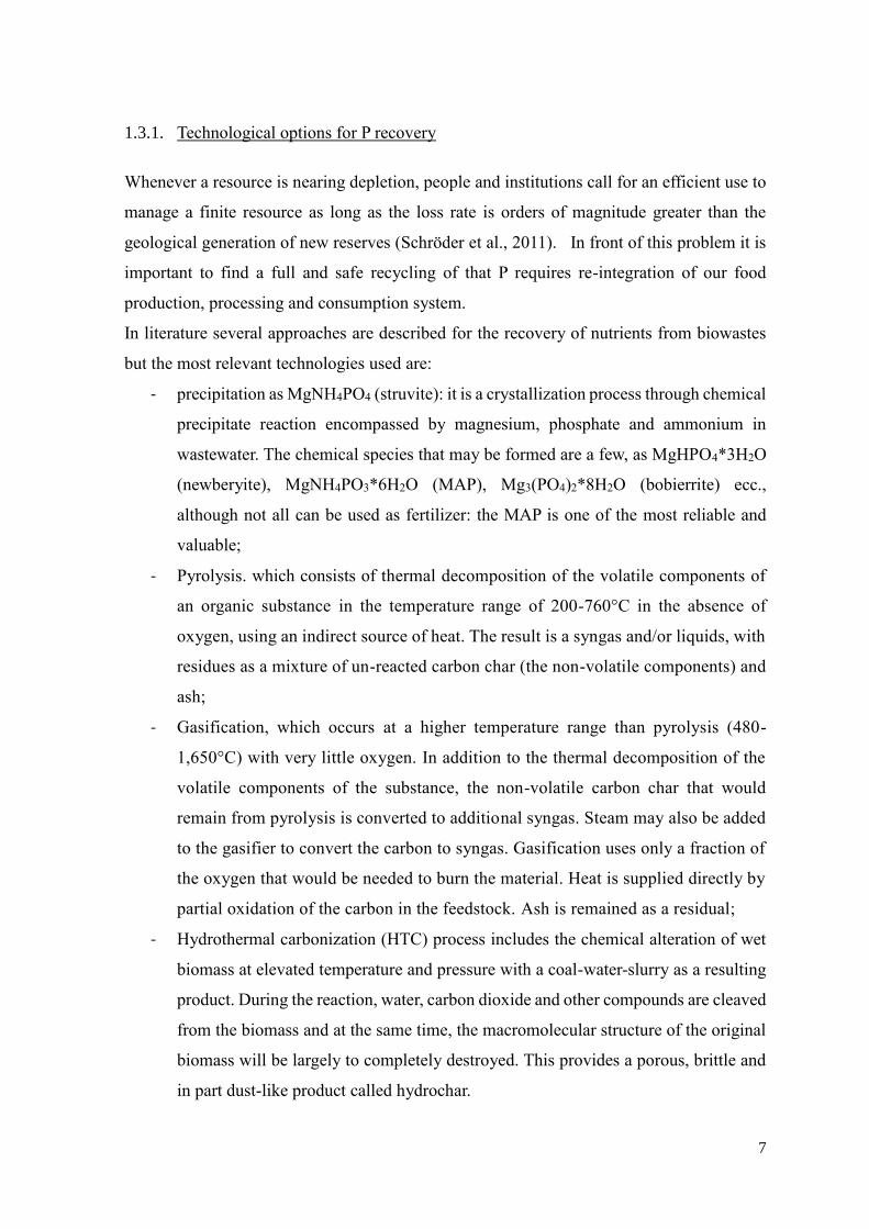
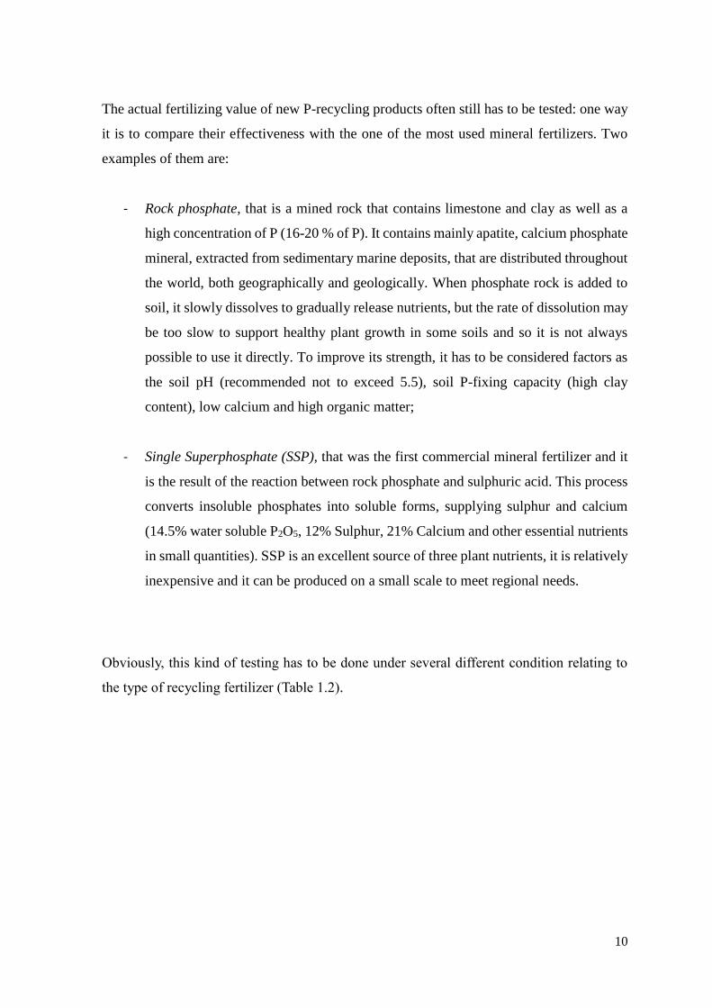
Figure 2.15 Precipitation of Fe in the solutions…….……………………………………………..32

Figure 2.16 Ferrihydrite gels………………………. ...................................................................... 32

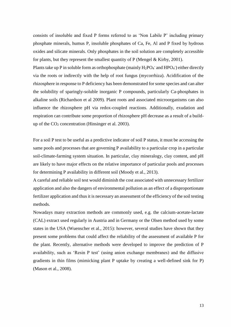
Figure 2.17 Material needed to shape the disks…………………………………………………..32

Figure 2.18 Ferrihydrite disks……………………… ..................................................................... 32

Figure 2.19 The gels solution spreads left and right by pipetting from the middle. ........................ 34

Figure 2.20 Some drops of water are added on the top of the glass plate to see better the gel. ...... 34

Figure 2.21 DGTs ready and arranged in a plastic bag in the fridge until the moment of the analysis

.......................................................................................................................................................... 34

Figure 2.22 DGTs device with plexiglas frame……………………………………………………35

Figure 2.23 DGTs device with soil on the top…….. ....................................................................... 35

Figure 2.24 After 24 h the soil is removed from the device. ........................................................... 35

Figure 2.25 Sample eluates on the plate shaker. ............................................................................. 35

Figure 2.26 Pots labelled………..…………………………………………………………………37

Figure 2.27 Pot with felt cover at the bottom. ................................................................................. 37

Figure 2.28 Soil crushed with hamme……………………………………………………………..37

Figure 2.29 Sieve 4 mm………………….. .................................................................................... 37

Figure 2.30 Rye grass seeds. ........................................................................................................... 39

Figure 2.31 Rye grass seeds spread around the surface of the pot. ................................................. 39

VI

Figure 2.32 Seeds begin to push tiny sprouts through the soil. ....................................................... 40

Figure 2.33 Rye grass in the middle phase of growth. In the pots were added bamboo sticks as a

supporter for the leaves. ................................................................................................................... 42

Figure 2.34 ICP-MS (Perkin Elmer)……………………………………………………………….45

Figure 2.35 Samples got in the position for the analysis……………………………………………45

Figure 2.36 Digestion tubes and acids…..………………………………………………………….46

Figure 2.37 Ceramic digestion tubes with lids and sensor………………………………………..46

Figure 2.38 Microwave digester Anton Paar - Multiwave 3000. .................................................... 46

Figure 2.39 Sample digested: the yellow one corresponding to the AR digestion, the one

corresponding to the HNO3 + H2O2 digestion…….. ........................................................................ 46

Figure 2.40 Illustration of the concept of detection and quantification limit by showing the

theoretical normal distributions associated with blank, detection limit and quantification limit level

samples. LOD is defined as 3 * standard deviation of the blank, and at the LOQ defined as 10 *

standard deviation of the blank. For a signal at the LOD, the alpha error (probability of false positive)

is small (1%). However, the beta error (probability of a false negative) is 50% for a sample that has

a concentration at the LOD (red line). This means a sample could contain an impurity at the LOD,

but there is a 50% chance that a measurement would give a result less than the LOD. At the LOQ

(blue line), there is minimal chance of a false negative. .................................................................. 48

Figure 3.1 P extracted from soil sample fertilized by 13 amendments with the CAL method. The

amount is expressed in mgP/kg DM and it is the mean value of experimental replicates (n=3). Error

bars indicate standard deviation of them. ......................................................................................... 53

Figure 3.2 Extractable soil P fraction from soil sample fertilized by 13 amendments with the CAL

method. The amount is expressed in mg P/kg DM and the first bar (brighter colour) belongs to the

control sample. The values are the average of experimental replicates (n=3) and the error bars indicate

standard deviation of them. .............................................................................................................. 55

Figure 3.3 DGT measurements (µgP l-1) on the gel for one type of soil fertilized with 13 type of

fertilizers. The two series of data are related to the two different incubation of time. The two bars in

brighter color belong to the control sample. Error bars indicate the standard deviation of experimental

replicates (n=3). ................................................................................................................................ 56

Figure 3.4 Biomass weight for each type of fertilizer and for the control sample. The control sample

has a brighter colour to underline the difference between the other. Error bars are the standard

deviation of experimental samples (n=3). ........................................................................................ 58

Figure 3.5 The histogram shows the P up taking by the plant in the 13 cases in which the soil was

fertilized with diverse fertilize; it is also shown the control amount (in a lighter colour) to catch better

an increase of the uptaking. The harvest was done after 6 weeks of growth. The values are the mean

between three experimental samples (n=3) and the error bars represent the standard deviation of

them. ................................................................................................................................................. 59

Figure 3.6 The graph shows the possible linear correlation between the plant P uptake measured

with the ICP-OES (mgP/pot) at increasing of detected P with DGT device in 5 days (µgP/l)..60


with the ICP-OES (mgP/pot) at increasing of detected P with DGT device in 20 days (µgP/l)..60


with the ICP-OES (mgP/pot) at increasing of extractable soil P (mgP/kg) revealed by Olsen method

with 5 days of incubation……………………………………………………………………..60


with the ICP-OES (mgP/pot) at increasing of extractable soil P (mgP/kg) revealed by CAL method

VII

with 5 days of incubation. The calibration line, with its corresponding parameter R2, was calculated

with Excel......................................................................................................................................... 60

Figure 3.10 Diagram of the estimated value Ŷ by the correlation line versus the residue ɛ , in DGT´s

case with 5 days of soil incubation……………………………………………………………63

Figure 3.11 Diagram of the estimated value Ŷ by the correlation line versus the residue ɛ , in DGT´s

case with 20 days of soil incubation…………………………………………………………63

Figure 3.12 Diagram of the estimated value Ŷ by the correlation line versus the residue ɛ, in Olsen

method´s case……………………………………………………………………………………...63

Figure 3.13 Diagram of the estimated value Ŷ by the correlation line versus the residue ɛ , in CAL

method´s case ................................................................................................................................... 63

Figure 3.14 Diagram of the predictor x versus the residue ɛ, in DGT´s case with 5 days of soil

incubation…………………………………………………………………………………………..64

Figure 3.15 Diagram of the predictor x versus the residue ɛ, in DGT´s case with 20 days of soil

incubation…………………………………………………………………………………………..64

Figure 3.16 Diagram of the predictor x versus the residue ɛ, in Olsen method´s case…………64

Figure 3.17 Diagram of the predictor x versus the residue ɛ, in CAL method´s case. .................... 64

Figure 3.18 The histogram has three different bars for every fertilzers: the two bars in grey darker

are the concentration of V by the Aqua Regia digestion, instead the bars in brighter grey are the

concentration of V by HNO3-H2O2. All the values are expressed in mgV/ kgP2O5. The Error bars

represent the standard deviation of experimental samples (n=3). .................................................... 66


are the concentration of Cr by the Aqua Regia digestion, instead the bars in brighter grey are the

concentration of Cr by HNO3-H2O2. All the values are expressed in mgCr/ kg. The Error bars

represent the standard deviation of experimental samples (n=3). The line blue means the threshold

amount of the compost regulation and the yellow line means the threshold value of the EBC

regulation.......................................................................................................................................... 67


are the concentration of Ni by the Aqua Regia digestion, instead the bars in brighter grey are the

concentration of Ni by HNO3-H2O2. All the values are expressed in mgNi/ kg. The Error bars


amount of the compost regulation, the red line is for the German Legislation and the green one is for

the Swiss one. ................................................................................................................................... 68

Figure 3.21 The histogram has three different bars for every fertilizers: the two bars in grey darker

are the concentration of Cu (63) by the Aqua Regia digestion, instead the bars in brighter grey are

the concentration of Cu (63) by HNO3-H2O2. All the values are expressed in mg Cu/ kg. The Error

bars represent the standard deviation of experimental samples (n=3). The blue line means the

threshold amount of the compost regulation and the yellow line is for the EBC regulation. ........... 69







are the concentration of Zn (66) by the Aqua Regia digestion, instead the bars in brighter grey are

the concentration of Zn (66) by HNO3-H2O2. All the values are expressed in mg Zn/ kg. The Error

VIII









are the concentration of As by the Aqua Regia digestion, instead the bars in brighter grey are the

concentration of As by HNO3-H2O2. All the values are expressed in mg As/kg. The Error bars

represent the standard deviation of experimental samples (n=3). The yellow line represents the EBC

regulation.......................................................................................................................................... 73


are the concentration of Cd (111) by the Aqua Regia digestion, instead the bars in brighter grey are

the concentration of Cd (111) by HNO3-H2O2. All the values are expressed in mg Cd/ kg. The Error

bars represent the standard deviation of experimental samples (n=3). The blue lines represent the

regulation for the compost, instead the yellow line the EBC regulation. ......................................... 74





regulation for the compost, instead the yellow line the EBC regulation. ......................................... 75


are the concentration of Pb by the Aqua Regia digestion, instead the bars in brighter grey are the

concentration of Pb by HNO3-H2O2. All the values are expressed in mg Pb/ kg. The Error bars

represent the standard deviation of experimental samples (n=3). The blue line represents the

regulation for the compost................................................................................................................ 76

Figure 4.1 Box plot of CAL and Olsen data series: the bottom and the top of the box are the first and

the third quartiles, and the band inside is the second quartile. The end of the whiskers is the inferior

and superior limit (corresponding to the minimum and maximum values of each data series). ...... 78

Figure A.1 Ryegrass seeds in germination………………………………………………………...90

Figure A.2 Pot with MSS BC 3………………………………………...………………………….91

Figure A.3 Pot with SSP………………………. ............................................................................. 91

Figure A.4 Pot with MSS BC………………………………………………………………………91

Figure A.5 Pot with Chicken manure .............................................................................................. 91

IX

List of tables

Table 1.1 Classification of soil P-contents and fertilization recommendations in Germany

(VDLUFA-Standpunkt Phosphor). The study of the P plant supply was done by the CAL method. 6

Table 1.2 Samples of possible fertilizer recommendations of P-recycling products. ...................... 11

Table 2.1 List of fertilizers studied for their P availability. NA: not analyzed................................ 18

Table 2.2 Selected characteristics of the soil tested. ....................................................................... 21

Table 2.3 Weight of the wet and air dry soil used for the CAL extraction. ................................ 22-23

Table 2.4 The weight of the wet and air dry soil used for the Olsen extraction. ........................ 25-26

Table 2.5 The stoichiometric quantities for the preparation of the solution. ................................... 27

Table 2.6 Preparation of carbon solution corresponding number of extractions (360 µl for each

sample). ............................................................................................................................................ 27

Table 2.7 P content expressed in % for dry matter basis, dry factor and the mg to add to the paste

(weight soil) for each type of fertilizer. ............................................................................................ 29

Table 2.8 Volume of solution and of reactants for thick diffusive gels. .......................................... 33

Table 2.9 Volume of solution and of reactants for thin diffusive gels. ........................................... 33

Table 2.10 The table contains the features of the diffusive layer, the time of deployment and the

volume of the eluate. ........................................................................................................................ 36

Table 2.11 The table above contains the amount of fertilizer (mg) for pot needed to have 100 mgP

in one kg of soil. ............................................................................................................................... 38

Table 2.12 Light density received by the photosynthetically active radiation in 5 different days. . 40

Table 2.13 The abundances and their corresponding interferences of the trace elements’ isotopes

analyzed....................................................................................................................................... 43-44

Table 2.14 The table below reports the statistical parameters of mean and standard deviation (SD)

and the LOD and LOQ of all the trace elements considered. ........................................................... 49

Table 2.15 In the table are reported all the regulations taken into account in this research and the

feedstocks that they are concerned. For each of them there are the trace elements’ threshold value

expressed in mgelement/kgsoil or mgelement/kgP2O5 ........................................................................... 50-51

Table 3.1 Concentration of P measured with DGT for the CMBC, SSP and MAP samples in the two

different period of incubation. .......................................................................................................... 57

Table 3.2 List of the intercept (b0) and the angular coefficient (b1) for the lines estimated by the

statistical tools of Excel, regarding all the chemical methods analysed in this research ................. 62

Table 4.1 The value of the statistical parameters used in the box plot

diagram………………………………………………………………………………………….87-89

Table A.2 Volume needed for the preparation of the calibration standard solutions in the CAL

method. ............................................................................................................................................. 94

Table A.3 Volume needed for the preparation of the calibration standard solutions in the DGT

method. ............................................................................................................................................. 94

Table A.4 This list declares only some of the trace elements studied in the research of Krüger in the

2014. For each of them is noted its minimum, its mean and its maximum concentration expressed in

mgelement/kgDM . ............................................................................................................................... 96

X

List of Abbreviations

AR Aqua Regia

As Arsenic

BGSL Biogas slurry

C Carbon

CAL Calcium-Acetat-Lactat

Cd Cadmium

CMBC Chicken Manure Biochar

CM Chicken Manure

Cr Chromium

Cu Copper

CV Coefficient of Variation

DGT Diffusive Thin Gels

Fe Iron

HQ High Quality

HTC Hydrothermal carbonization

ICP-MS Inductively Coupled Plasma Mass Spectrometry

ICP-OES Inductively Coupled Plasma Optical Emission Spectrometry

LOD Limit of Detection

LOQ Limit of Quantification

MAP Magnesium Ammonium

MBM Meat & Bonemeal

MBM-BC Meat & Bonemeal Biochar

MSS A1 Municipal sewage sludge ash 1

MSS A2 Municipal sewage sludge ash 2

MSS BC 1 Municipal sewage sludge 1

MSS BC 2 Municipal sewage sludge 2

MSS BC 3 Municipale sewage sludge 3

N Nitrogen

Ni Nickel

P Phosphorus

XI

Pb Lead

PE Polyethylene

QC Quality Control

QM Quality Monitor

RF Recycled Fertilizer

RP Rock Phosphate

SD Standard Deviation

SOW Stabilized Organic Waste

SSP Single Superphosphate

V Vanadium

WHC Water Holding Capacity

Zn Zinc

XII

Table of contents

1. INTRODUCTION .................................................................................................................... 1

1.1. The objectives of the research................................................................................. 1

1.2. P supply in Europe .................................................................................................. 3

1.3. P availability from fertilizers .................................................................................. 4

1.3.1. Technological options for P recovery ........................................................................ 7

1.3.2. Types of recycling fertilizers ...................................................................................... 8

1.4. Soil tests ................................................................................................................ 11

1.4.1. Calcium Acetate Calcium Lactate method (CAL) ................................................... 14

1.4.2. Olsen method............................................................................................................ 14

1.4.3. Diffusive Gradient in Thin film (DGT) .................................................................... 15

1.5. Analysis of possible contamination in the P fertilizers ......................................... 16

2. MATERIAL AND METHODS ............................................................................................. 18

2.1. Characteristics of fertilizers .................................................................................. 18

2.2. Sample preparation ............................................................................................... 20

2.3. Characteristics of the soil ...................................................................................... 20

2.4. Soil P tests ............................................................................................................. 21

2.4.1. Calcium Acetate Calcium Lactate method (CAL) ................................................... 21

2.4.2. Olsen method............................................................................................................ 25

2.4.3. Diffusive Gradient in Thin film (DGT) .................................................................... 29

2.5. Pot trial .................................................................................................................. 36

2.6. Analysis of any potential release of contaminants ................................................ 43

2.6.1. Preparation of the samples and the standards ........................................................... 45

2.6.2. Instrumental setting and calibration ......................................................................... 47

2.6.3. Injection sequence and calculations ......................................................................... 47

2.7. Statistics ................................................................................................................ 52

XIII

3. RESULTS ................................................................................................................................ 53

3.1. Calcium Acetate Calcium Lactate (CAL) ............................................................. 53

3.2. Olsen method ........................................................................................................ 54

3.3. Diffusive Gradient in Thin Films .......................................................................... 55

3.4. Plant growth .......................................................................................................... 57

3.5. Correlation between the pot trial and the soil P test ............................................. 59

3.6. Analysis of the possible contaminations of the recycling fertilizers .................... 65

4. DISCUSSIONS ....................................................................................................................... 77

4.1. Comparison between the two extraction methods ................................................ 77

4.2. DGT method ......................................................................................................... 79

4.3. Evaluation of the efficiency of the 13 recycled fertilizers .................................... 81

4.4. Possible contamination released by the fertilizers ................................................ 82

5. CONCLUSIONS..................................................................................................................... 85

APPENDIX I ................................................................................................................................... 87

APPENDIX II ................................................................................................................................. 92

APPENDIX III ............................................................................................................................... 96

REFERENCES ............................................................................................................................... 97

WEB RESOURCES ..................................................................................................................... 101

1

1. INTRODUCTION

1.1. The objectives of the research

Phosphorus is the eleventh most abundant element in the earth’s crust, which contains

around 5–10 × 108 million tons (Mt) of P (Cooper et al., 2011), and it represents an essential

and irreplaceable element for living organisms on earth: it is essential for life to grow and

function, and thus crucial for our food system and own health (Cordell et al., 2009). The

element P cannot be substituted since it is part of biological processes such as reproduction

(DNA), energy supply (ATP) and body structure (bones, teeth) (Oelkers and Valsami-Jones,

2008).

Phosphorus can be distinguished between primary and secondary P: the former is based on

mined P rock sourced from the geological cycle with a timescale of millions of years, the

latter is based on organic materials renewed in an anthropogenic timescale and mostly

managed within the anthroposphere (e.g. food, waste, excrements) (Van Dijk et al., 2016).

All chemical fertilizer and feed P are derived from phosphate-rich rocks but they are finite

and non-renewable resources on a human time scale, therefore their global size has been a

major source of concern recently. Recent assessments suggest that the reserves could be

exhausted within 50-400 years depending on P supply and demand dynamics (Reijnders

2014; Sattari et al.; 2012; Scholz and Wellmer, 2013). The 75% of them are located in

Morocco and Western Sahara (USGS, 2014) whereas Europe is poor in those deposits, with

the majority located in Finland (de Ridder et al., 2012).

Such predictions highlight the need to both use P efficiently and recycle it to close the cycle

of supply and demand (the two main options for closing the cycle are (1) to realign P inputs

(such as the chemical fertilizer P, followed by imported food products, animal feed and non-

food products) and (2) to recover/recycle P from food processing waste, non-food waste,

municipal waste and manure (Schoumans et al., 2015). To this end, several processes exist,

including different biological, thermal and/or chemical processes. The wide variety of new

fertilizers differ in their P content and availability (Cabeza et al., 2011).

2

Once a fertilizer is applied to the soil, it has to enhance its fertility: the ability to produce

healthy and plentiful plants is improved by the release of macro- and/or micronutrients

contained in the fertilizer in case of deficiency in the soil. In order to assess the efficiency of

a fertilizer it is required to use accurate methods. Since plants absorb P from the soil solution,

to become effective a P fertilizer must dissolve in soil water. Once the P dissolves in the soil

solution it may subsequently be adsorbed to the soil particles or precipitate. These forms stay

in equilibrium with soil solution and remain available to the plant, but often at low rate,

depending on the soil P level.

The amount of a fertilizer that dissolves and reacts with the soil can be estimated using some

form of extraction. Even if the bioassay method (greenhouse or field experiment) is the most

reliable approach, there is a number of standard and novel soil tests that can predict plant P

availability, but their accuracy still needs to be evaluated in the context of P recycling

fertilizers.

Figure 1.1 Map about the reserves’ distribution of rock phosphate in the world (US geological survey

2014).

The objectives of my research are:

- To assess the prediction of P availability from 13 recycling fertilizers obtained from

different resources: they consist of chicken manure, meat and bone meal, biogas

slurry and their respective biochars, sewage sludge biochars and ash, single

superphosphate (SSP) and magnesium ammonium phosphate (MAP). The

assessment is done with a bioassay conventional test and some novel alternative

3

methods as Calcium Acetate – calcium Lactate (CAL), Olsen, and the Diffusive

Gradients in Thin films (DGT).

- To assess the efficiency of P fertilizers used and to measure any potential release of

contaminants in the plants and in the soil.

1.2. P supply in Europe

Currently, within the European Union (EU-27), a yearly total amount of 1 to 1.5 Mt of P is

applied on agricultural or horticultural land: more than 95% in the form of inorganic

fertilizers and manure, between 2005 and 2008 (EUROSTAT), and in an insignificant part

as P input from other sources (e.g. sewage sludge, industrial waste, compost etc.). Then,

about half of the P applied as fertilizer in Europe has organic origin (Slurry, Farm Yard

Manure, digestates from anaerobic digestion).

To provide an understanding of the use of P as agricultural nutrients, it is useful to have a

look at the Gross Phosphorus Balance. It is intended to be an indicator of the potential threat

of surplus or deficit of P in agricultural land, analyzing factors determining the nutrient trend

over the time. The balance is calculated between inputs (consumption of fertilizers, manure

and other inputs) and outputs (removal of P with harvest of crops, with the grazing of fodder

and crop residues removed from the field) of P to the agricultural soil. The data presented in

the table are calculated from basic data from various data sources (available in Eurostat)

multiplied with coefficients to derive the nutrient content. The basic data used include the

consumption of inorganic and other organic fertilizers (excluding manure) (tons), livestock

population (1000 heads), manure imports, withdrawals and stock changes (tons), crop and

fodder production (tons), crop residues removed from the field (tons), use of seeds and

planting materials planted in the soil (tons), area of leguminous crops (1000 ha), area of

arable land, land under permanent crops and permanent grassland (1000 ha). Countries may

have used different types of data sources for these data and they have estimated coefficients

based on measurements, scientific research, expert judgment, default values, etc.

(EUROSTAT).

4

Figure 1.2 Graph of Phosphorus balance between inputs and outputs of P in the agricultural land;

the data are taken from Eurostat and they are expressed in kgP/ha (EUROSTAT).

The bar-graph below shows large differences between the countries: this depends on several

factors such as availability of funds in agriculture (low rates in eastern European countries),

density of livestock, export of agricultural products P fertilizers sales, official fertilizing

recommendations, advertising of producers and retailers, specific restrictions e.g. for organic

farming, and others. As can be seen, in the year of 2014 only two countries, Malta and

Cyprus, have a high P surplus; on the other hand, Bulgaria and Estonia have the largest P

deficit.

1.3. P availability from fertilizers

Justus von Liebig (1803-1878) demonstrated as early as in 1840, that P can also be used

from mineral sources (phosphate rocks): his studies on mineral plant nutrition led to a change

in fertilizer practices and an increasing of the crops yield by the factor 5 to 10, since then.

The fertilization with bone meal is used since the beginning of the 19th century with the

consecutive improvement by adding phosphoric acid (P-REX, European Commission).

-10

-5

0

5

10

15

20

25

30

35

P b

ala

nce

(k

gP

/ha

)Gross Phosphorus Balance (2014)

5

Not all the fertilizer applied is immediately available for plants due the fact that more than

80% of the P fertilizer may be strongly absorbed or precipitated in the soil (Sample et. al.

1980; Sanyal & De Datta 1991).

Figure 1.3 The role of mineral P-fertilizers in crop nutrition. Broad spread P fertilizer has a

theoretical efficiency of 13% for an annual crop. Placed fertilizer can have 25% efficiency in one

vegetation period (Agricultural Committee, 1980).

In soils where the P availability is low P and its exploitation is from 5 to 15% in general,

(Agricultural Comitee of ISMA, 1980), possibly because of stable bonds. P amounts

provided in the form of fertilizer must be much greater than the annual requirements of the

crops. On the contrary, once the optimal level is reached, it is needed to be replaced only the

amount of P exported, at least for cereals (Johnston et al., 2014). If fertilizer is broadcasted

on soil, up to 13% of its P can be taken up by plants. Banding (e.g. under foot placing when

sowing row crops) can increase this share to 25% (Agricultural Committee of ISMA, 1980).

It is required at least the amount equivalent to what was exported with the harvest in order

to keep or increase available P. Phosphorus fertilizer application is decided in relation with

soil

1200 kg soil with 0.3%

P2O5

80 kg

P2O5

40 kg

P2O5

fertilizer placed

fertilizer

10 kg 60 kg 10 kg

CROP

80 kg

6

the P-content of soil. For example, in Germany and also in other countries of Europe, there

is a classification according to the contents (Table 1.1) that suggests how to manage the

fertilization. Soils in category E do not need any treatment, whereas the rest yes: from the

category A that needs a highly input of P to category D that need a greater P output to deplete

the soil P content.

Category CAL-P (mg P/100 g soil) Fertilization

A

B

C

D

E

≤ 2.0

2.1 - 4.4

4.5 - 9.0

9.1 – 15.0

≥15.1

Highly increased fertilization

Increased fertilization

Maintenance fertilization

Reduced fertilization

No fertilization

Table 1.1 Classification of soil P-contents and fertilization recommendations in Germany

(VDLUFA-Standpunkt Phosphor). The study of the P plant supply was done by the CAL method.

Not more than 3 to 6% of all arable land in Germany (375,000 - 750,000ha) are currently

classified as category “A” (Römer 2013, a). Similar numbers have been found for

Switzerland (BUWAL, 2004).

To assess if a fertilizer has a good efficiency several aspects are taken into account: their

solubility in water and stepwise in weak to strong acids and physical, chemical and biological

P – soil – plant interactions. For instance, Myint (2005) has shown that fine ground raw

phosphate rocks do not contribute to plant nutrition within 20 years when the pH value of

the soil is between 6 and 7 which applies for most soils in Europe.

Furthermore, as Classen affirmed in 2010, a fertilizer with a good response has to be

experienced within a financially recognizable time.

According to current knowledge, the main influencing factors to develop fertilizer

recommendations for P-recycling products are: type of fertilizer and chemical

characteristics, soil nutritional status and soil pH-value.

7

1.3.1. Technological options for P recovery

Whenever a resource is nearing depletion, people and institutions call for an efficient use to

manage a finite resource as long as the loss rate is orders of magnitude greater than the

geological generation of new reserves (Schröder et al., 2011). In front of this problem it is

important to find a full and safe recycling of that P requires re-integration of our food

production, processing and consumption system.

In literature several approaches are described for the recovery of nutrients from biowastes

but the most relevant technologies used are:

- precipitation as MgNH4PO4 (struvite): it is a crystallization process through chemical

precipitate reaction encompassed by magnesium, phosphate and ammonium in

wastewater. The chemical species that may be formed are a few, as MgHPO4*3H2O

(newberyite), MgNH4PO3*6H2O (MAP), Mg3(PO4)2*8H2O (bobierrite) ecc.,

although not all can be used as fertilizer: the MAP is one of the most reliable and

valuable;

- Pyrolysis. which consists of thermal decomposition of the volatile components of

an organic substance in the temperature range of 200-760°C in the absence of

oxygen, using an indirect source of heat. The result is a syngas and/or liquids, with

residues as a mixture of un-reacted carbon char (the non-volatile components) and

ash;

- Gasification, which occurs at a higher temperature range than pyrolysis (480-

1,650°C) with very little oxygen. In addition to the thermal decomposition of the

volatile components of the substance, the non-volatile carbon char that would

remain from pyrolysis is converted to additional syngas. Steam may also be added

to the gasifier to convert the carbon to syngas. Gasification uses only a fraction of

the oxygen that would be needed to burn the material. Heat is supplied directly by

partial oxidation of the carbon in the feedstock. Ash is remained as a residual;

- Hydrothermal carbonization (HTC) process includes the chemical alteration of wet

biomass at elevated temperature and pressure with a coal-water-slurry as a resulting

product. During the reaction, water, carbon dioxide and other compounds are cleaved

from the biomass and at the same time, the macromolecular structure of the original

biomass will be largely to completely destroyed. This provides a porous, brittle and

in part dust-like product called hydrochar.

8

Atkinson et al. (2010) affirmed that the P availability of biochars is increased due to a higher

temperature of organic matter and Kammann et al. (2011) reported that the highly porous

structure of biochars is important in encouraging microbial activity in soils.

1.3.2. Types of recycling fertilizers

As it was said before, recycling of P from waste materials by chemical or thermal processes

it is important. The P-products that could be obtained are several depending on the making

procedure:

- Bonemeal and Chicken manure Biochars are the respective biochars of the organic

fertilizer Bonemeal and Chicken manure (rich of Nitrogen with a good amount of

Potassium) that were obtained by the process of pyrolyzation at 400°C of the

feedstock described above. The method was done in an experimental lab reactor with

nitrogen as a flush gas: those solid residues are safer because of the disinfection by

the high temperature;

- Biogas slurry is an organic and liquid fertilizer (93% water and 7% of dry matter, of

which 4.5% is organic matter and 2.5% inorganic matter) produced by biogas

systems and easily collected in the outlet of the digester with a bucket. It can be used

to fertilize crops directly or added with other organic materials and synthetic

fertilizers. The digested biogas slurry also contains considerable amount of

macronutrients (phosphorus, potassium, nitrogen) and micronutrient (zinc, iron,

manganese and copper) required for plant growth (Kumar et al., 2015);

- Struvite is a fertilizer-grade struvite (NH4MgPO4·6H2O) is one recovered P with a

high P content, frequently produced as a by-product of wastewater treatment: within

treatment plants where there are rapid pressure changes, it forms a scale on lines and

clogs pipes (Jaffer et al. 2002). However, controlled struvite precipitation can be

triggered in specialized reactors by manipulation of the sludge digestion process to

overcome these problems (Baur 2009). This can produce struvite granules that are

useable as a magnesium ammonium phosphate fertilizer product for agriculture,

9

whilst also reducing plant effluent P concentrations discharged to watercourses (Baur

2009; Schauer et al. 2011).

Struvite, as a less soluble slow release fertilizer, could provide a longer term source

of P for crop growth than readily soluble forms of P, thus more closely matching the

plant’s demand for P later in the growing season and increasing its efficiency of use

(Withers et al. 2014);

- Municipal Sewage Sludge biochar and ash: The sewage sludge is an impending

byproduct of wastewater treatment and its management has become a high problem

in Europe over the last years due to legislation and environmental issues. The raw

sludge is known for its high nutrient content, organic matter and trace elements that

are essential for plant growth and yield (Wong et al., 1995, Keuthale et al. 2005).

Application of sludge has been observed to improve the physico-chemical and

biological properties of soils which in turn facilitates better growth of plants. The

biomass yields of plants grown on sludge-amended soils have also been observed to

increase: The shoot length, root length, biomass and total chlorophyll contents of

plants increase with increasing rate of sewage sludge application (Kumar et al., 2004,

Aggelides et al., 2000). It was demonstrated by Mtshali (2004) that all the sample

studied have large organic matter content but the anaerobically digested sludge

contains the highest nutrient content.

Recently, thermo-chemical treatments, as gasification and pyrolysis, have been

developed; those methods represent an opportunity to recover nutrient from this

waste and to use them in the fertilization of agricultural land. The study conducted

by Liu et al. (2014) showed that the pyrolitic conversion of the raw sludge could be

feasible to produce a fertilizer. The biochars improved the soil productivity (increase

of yield of 46%) and raised the total and available P and K concentrations meeting

the relevant agronomic standards.

Lin et al. (2007) and Chen et al. (2009) studied the combination of ISSA (Incinerated

Sewage Sludge Ash) with Ca(OH)2 or cement for soil stabilization applications.

ISSA has also been used as mineral filler in asphalt production replacing limestone

(Al Sayed et al. 1995).

10

The actual fertilizing value of new P-recycling products often still has to be tested: one way

it is to compare their effectiveness with the one of the most used mineral fertilizers. Two

examples of them are:

- Rock phosphate, that is a mined rock that contains limestone and clay as well as a

high concentration of P (16-20 % of P). It contains mainly apatite, calcium phosphate

mineral, extracted from sedimentary marine deposits, that are distributed throughout

the world, both geographically and geologically. When phosphate rock is added to

soil, it slowly dissolves to gradually release nutrients, but the rate of dissolution may

be too slow to support healthy plant growth in some soils and so it is not always

possible to use it directly. To improve its strength, it has to be considered factors as

the soil pH (recommended not to exceed 5.5), soil P-fixing capacity (high clay

content), low calcium and high organic matter;

- Single Superphosphate (SSP), that was the first commercial mineral fertilizer and it

is the result of the reaction between rock phosphate and sulphuric acid. This process

converts insoluble phosphates into soluble forms, supplying sulphur and calcium

(14.5% water soluble P2O5, 12% Sulphur, 21% Calcium and other essential nutrients

in small quantities). SSP is an excellent source of three plant nutrients, it is relatively

inexpensive and it can be produced on a small scale to meet regional needs.

Obviously, this kind of testing has to be done under several different condition relating to

the type of recycling fertilizer (Table 1.2).

11

Fertilizer product Suitable fertilizing scheme

Sewage sludge Application according to official

guidelines, plant availability of P reduced

with high Fe content

Struvite Generally suitable for application in

category B, C and D, preferably every 3

years and not placed at the time of seeding

Untreated ash Suitable for very acidic soils

Thermo-chemically treated ash (ASH

DEC, Na2CO3)

For acidic as well as neutral soils

Chemically treated ash (LEACHPHOS) Good plant availability, better efficiency on

acidic soils

Thermo-metallurgic treatment (Mephrec®) Lower plant availability in the first year

than other ash-based products. Unknown

long-term effect. Possibly suitable as slow-

release fertilizer to maintain P contents in

soil.

Table 1.2 Samples of possible fertilizer recommendations of P-recycling products.

1.4. Soil tests

Ideally a soil test should measure the form of P that is available to the plant, reflecting

diffusional supply from the soil solution and its resupply from the soil solid phase

irrespectively of soil type.

The amount of P extracted by a soil P test is dependent on the soil P pool(s) and process(es)

to which the soil P test is responsive. The soil P pools can be gestated as ‘solution P’, ‘sorbed

P’, ‘mineral P’ and ‘organic P’ (figure 1.4). All of these P pools are in equilibrium with

orthophosphate in the soil solution by the processes of desorption-adsorption (in the case of

sorbed P), dissolution-precipitation (in the case of mineral P), and mineralization-

immobilization (in the case of organic P). Mineral P comprises solid-phase P compounds of

various specific surface areas and structural organizations: they interact with solution P

12

through dissolution-precipitation reactions governed by the solubility products of the P

compounds and the rate of dissolution. Organic P comprises various organic P compounds

such as phytates that occur in plant residues and soil organic matter: the mineralization of

organic P or immobilization of inorganic P by microbial processes is dependent on the C:N:P

ratio of the soil organic matter and plant residues, as well as other factors. Sorbed P is that

quantity of P adsorbed onto the surfaces of iron and aluminium oxy-hydroxides and calcium

carbonates by electrostatic and covalent bonding: the amount of P adsorbing or desorbing

from surfaces depends on the number of sorption sites and the energy of adsorption (P buffer

capacity). Solution P is the ultimate source of P supply to the plant, primarily through the

process of diffusion, which is dependent on many factors including the P concentration

gradient between the root surface and the bulk soil solution, rate of P re-supply to solution

P as it withdrawn, the volumetric soil water content, soil P buffer capacity (change in the

quantity of soil P for a change in solution P concentration), and the connectivity of water

films in soil pores.

Figure 1.4 Soil P pools and processes: Sorbed P (P adsorbed onto the surfaces of Fe and Al oxy-

hydroxieds and calcium carbonate), Mineral P (fertilizer reaction products, apatites) and Organic P

(organic matter, microbial biomass).

P contents in arable soils vary between 0.02 and 0.1 % while in organic soils (moor, fen,

peat etc.) concentrations may be higher. Within the topsoil (0 - 30 cm depth) the total amount

may be 600 to 3000 kg of P ha-1. The major fraction is nearly inaccessible for plants, it

Sorption Desorption

Solution P Mineral P

Sorbed P

Dissolution

Precipitation

Mineralisation

e

Immobilisation

Organic P

Diffusion PLANT

13

consists of insoluble and fixed P forms referred to as ‘Non Labile P’ including primary

phosphate minerals, humus P, insoluble phosphates of Ca, Fe, Al and P fixed by hydrous

oxides and silicate minerals. Only phosphates in the soil solution are completely accessible

for plants, but they represent the smallest quantity of P (Mengel & Kirby, 2001).

Plants take up P in soluble form as orthophosphate (mainly H2PO4- and HPO4

-) either directly

via the roots or indirectly with the help of root fungus (mycorrhiza). Acidification of the

rhizosphere in response to P deficiency has been demonstrated for some species and can alter

the solubility of sparingly-soluble inorganic P compounds, particularly Ca-phosphates in

alkaline soils (Richardson et al 2009). Plant roots and associated microorganisms can also

influence the rhizosphere pH via redox-coupled reactions. Additionally, exudation and

respiration can contribute some proportion of rhizosphere pH decrease as a result of a build-

up of the CO2 concentration (Hinsinger et al. 2003).

For a soil P test to be useful as a predictive indicator of soil P status, it must be accessing the

same pools and processes that are governing P availability to a particular crop in a particular

soil-climate-farming system situation. In particular, clay mineralogy, clay content, and pH

are likely to have major effects on the relative importance of particular pools and processes

for determining P availability in different soil (Moody et al., 2013).

A careful and reliable soil test would diminish the cost associated with unnecessary fertilizer

application and also the dangers of environmental pollution as an effect of a disproportionate

fertilizer application and thus it is necessary an assessment of the efficiency of the soil testing

methods.

Nowadays many extraction methods are commonly used, e.g. the calcium-acetate-lactate

(CAL) extract used regularly in Austria and in Germany or the Olsen method used by some

states in the USA (Wuenscher et al., 2015): however, several studies have shown that they

present some problems that could affect the reliability of the assessment of available P for

the plant. Recently, alternative methods were developed to improve the prediction of P

availability, such as ‘Resin P test’ (using anion exchange membranes) and the diffusive

gradients in thin films (mimicking plant P uptake by creating a well-defined sink for P)

(Mason et al., 2008).

14

1.4.1. Calcium Acetate Calcium Lactate method (CAL)

This method was introduced by Schüller (1969) and it extracts only readily soluble and

exchangeable phosphate as well as easily dissolved Ca phosphates from fertilizers. The

research made by Wuenscher et al. (2015) showed that the mean value extracted was in the

range around or below 100 mg/kg soil. It could present some problems with soil with pH

below 6 because the extracted phosphate might get re-adsorbed on Al and Fe oxides

(Wuenscher et al., 2015). Zorn and Krause (1999) analyzed the effect of CaCO3 content in

the soil on the extraction capacity and they suggested that higher CaCO3 contents may

increase the pH in the extraction solution and diminish the effectiveness of the extraction.

1.4.2. Olsen method

The Olsen-P is the common name of the sodium bicarbonate (NaHCO3)-extractable

phosphorus in the method introduced by Olsen in 1954.

Pote (1996) and Turner (2004) affirmed the possibility to use it as a surrogate measure of

potential P loss through runoff. In the regions using the Olsen-P as the recommended soil P

test it is often a criterion in soil P indices for assessing risk of P loss and impact on surface

waters (Sharpley et al. 1994).

The OH- and HCO3- in the NaHCO3 solution decrease the concentration or activity of Ca2+

and Al3+, resulting in increased P solubility in soils: the high pH further enhances phosphate

desorption from Al and Fe oxide surfaces (Sims 2000, Schoenau and O’Halloran 2007). The

extractant is useful for both acid and calcareous soils as shown by Kamprath and Watson

(1980). In general, it is preferably used for calcareous soil, > 2% CaCO3 (Wuenscher et al.,

2015) in which increased calcium phosphate solubility results from the decreased Ca

concentration by the high concentration of carbonate ions and the precipitation of CaCO3. In

acid or neutral soils, the solubility of aluminium and iron phosphates increases as increased

OH- concentrations decreases the concentration of Al3+ by aluminate complex formation and

of Fe3+ by precipitation as the oxide. The increased surface negative charges and/or

decreased number of sorption sites on Fe and Al oxide surface at high pH levels could be

responsible for the desorption of sorbed P as well. Moody et al. (2013) proved this high

correlation with rate of P (FeO-P) and solution P and the low correlation with mineral P.

15

The method can be influenced by fertilizer and manure additions and it is not suitable for P

extraction from soils amended with relatively water-insoluble P materials such as rock

phosphate (Shoenau et al., 2008).

1.4.3. Diffusive Gradient in Thin film (DGT)

The Diffusive Gradients in Thin Film is a new technique that attempts to mimic the uptake

of the solutes by plant roots by providing a sink for the free orthophosphate ion (Mason et

al., 2013). Mason et al. (2010) concluded that DGT was able to predict P availability

throughout a wide range of soil types due to the measurement of P being obtained under

conditions that are close to those experienced by the plant root during P uptake. The

technique measures not only the concentration of the nutrient in the soil solution, but the

soil’s ability to resupply the nutrient to the solution from the solid phase. Furthermore, it

involves less physical disturbance than traditional extraction methods and works at more

“natural” solid-to-liquid ratios (Degryse et al. 2009). Because of all its good features, it is

expected to provide a very good or better assessment of plant nutrient availability compared

to traditional soil extraction tests.

The rate of P diffusion is dependent on the P concentration gradient between the root surface

and the bulk soil solution, the volumetric soil water content, the connectivity of water films

in soil pores and the P buffer capacity (Nye 1980). Moody et al. (2013) conducted a study to

understand what soil properties and processes determine P availability using a subset of

Australian soils. They demonstrated that the diffusive P supply is likely to be mainly

determined by the water-filled porosity, pore-size distribution and P buffer capacity:

anyway, only 40-62% of the variation in the DGT-P could be accounted for by soil

characteristics considered in this study, and it was supposed that DGT-P was also joining

other soil characteristics not investigated in that research that affect the diffusive supply of

P.

So, the method measures the time-averaged concentration in solution at the surface of the

DGT device CDGT (µg/l). The amount of P accumulated on the binding layer depends on the

concentration of P in the soil pore water as well as the rate at which P is supplied from the

soil phase into the pore water. So the mode of the measurement is by diffusion of available

P in the soil toward a P sink via a membrane which controls movement of P to the sink.

16

The capacity of the binding gel is limited and once it is exhausted it is not possible anymore

to assume it as an infinite sink. This may create problems in soils with very high nutrient

status or in soils which have recently been amended with manure or other fertilizers high in

P (Christel et al. 2014). In addition to the limited P-binding capacity, variation in elution

efficiency has been found to be a critical source of systematic and random error in the DGT

method (Kreuzeder et al. 2015). Although the use of the correct elution factor (fe) is crucial

for producing valid estimates of P bioavailability in solutions and soils (Christel et al., 2016),

it is considered to be 1 for P bound to ferrihydrite gels.

Due to the variety of different methods of P recycling and the fact that characteristics of

products are still subject to changes as a result of process adaptations, general conclusions

regarding P availability are difficult to draw. Pot or laboratory experiments have the

(fundamental) weakness, that no long term effects can be assessed and that biological and

chemical conversion processes in the soil can only be taken into account to a very limited

extent. This may lead to under-estimation of mid to long term P availability especially from

raw phosphate rocks or incineration ashes as these fertilizers may need intensive chemical

or biological conversion processes in order to become plant available (Römer, 2013b).

1.5. Analysis of possible contamination in the P fertilizers

Although fertilizers may produce a quick increase in crop yield, their use could lead to

contamination if they contain pollutants above the threshold value established for some

elements released in the soil (Cd, Br, …). The presence of such harmful elements could leach

into water bodies leading to water pollution or they can be dangerous for human health.

To determine the total content of possible contaminants in the samples Inductively Coupled

Plasma Mass Spectrometry (ICP-MS) is the standard technique in modern elemental

analytical chemistry. ICP-MS is an analytical technique that has the ability to detect

elemental ions and isotopic information: a large number of elements can be detected (Figure

1.5).

17

Figure 1.5 Elements determined by ICP-MS and approximate detection capability (Ruth 2005).

This machine has many advantages in comparison to the other spectroscopy technologies

e.g. ICP-OES, Graphite Furnace AA, ecc.):

- a high sensitivity because it can analyze the trace levels with detection limit at or

below the part per trillion (ppt);

- a fast detection: it is able to scan the mass spectrum from 3-250 atomic mass unit

(amu) in few seconds;

- it is capable to move from one mass to another with a high degree of precision (Tyler

et al., 1995).

An ICP-MS combines a high-temperature ICP (Inductively Coupled Plasma) source with a

mass spectrometer. The ICP source converts the atoms of the elements in the sample

(commonly inserted as an aerosol, either dissolved solid sample or by aspirating a liquid) to

ions that are then separated and detected by the mass spectrometer via the interface cones.

18

2. MATERIAL AND METHODS

2.1. Characteristics of fertilizers

In this thesis thirteen P-rich biowastes (subsequently referred to as fertilizers) were assessed.

They were treated with processes as pyrolysis, gasification, precipitation as MgNH4PO4 and

hydrothermal carbonization. They were selected to represent a broad range of potential P

sources for agriculture. Total P (Pt) content was analyzed by ICP-OES after microwave

digestion in aqua regia (100 mg sample, 4.5 ml 37 % HCl + 1.5 ml 65 % HNO3).

Additionally, total carbon (Ct) and nitrogen (Nt) of the materials originating from waste and

manures was analyzed by dry combustion in an elemental analyzer. Total P contents of the

fertilizers ranged from 19 to 142 mg g-1, and the C and N contents of the recycling materials

varied widely from 43.9 to 441.2 mg g-1 and 1.2 to 79.4 mg g-1 respectively.

Fertilizer Sample code P total C total N total

(mg g-1) (mg g-1) (mg g-1)

Meat & bone meal MBM 54.7 408.9 79.4

Meat & bone meal biochar MBM-BC 114.1 276.0 37.7

Chicken manure CM 22.4 371.4 32.5

Chicken manure biochar CM BC 43.7 371.4 24.0

Biogas slurry (solid fraction) BGSL 19.1 441.2 23.6

Municipal sewage sludge

biochar 1

MSS BC 1 90.6 314.5 44.1


biochar 2

MSS BC 2 68.8 237.9 24.6


biochar 3

MSS BC 3 92.1 NA NA

Municipal sewage sludge ash

1

MSS A 1 79.5 43.9 1.2

Municipal sewage sludge ash

2

MSS A 2 104.1 89.0 2.6

Rock phosphate RP 142.9 a NA NA

Single superphosphate SSP 95.0 a NA NA

Magnesium Ammonium

Phosphate

MAP 123.6 a NA NA a content based on air-dry condition

Table 2.1 List of fertilizers studied for their P availability. NA: not analyzed.

19

Bone meal: the sample used in this research was collected from Steirische

Tierkörperverwertungsgesellschaft m.b.H. & Co KG, Gabersdorf, Austria.

Chicken manure: it was provided by a farmer from Leithaprodersdorf (Austria).

Bone meal and Chicken manure Biochars: the respective biochars were obtained by the

process of pyrolyzation at 400°C of the feedstock described above. The method was done in

an experimental lab reactor with nitrogen as a flush gas: those solid residues are safer

because of the disinfection by the high temperature.

Biogas slurry: we used a biogas slurry from production plant in Bruck/Leitha in Lower

Austria. The feed material for biogas production were food wastes and agricultural wastes.

The anaerobic digestate had a dry mass of about 5wt% and a pH of 8. It was freeze dried and

the solid residue was pyrolyzed. The amount of biochar was not sufficient to perform the pot

experiment.

Struvite (MAP): our MAP is a commercial product (Berliner Pflanze) produced by

precipitation in a wastewater treatment plant in Berlin, Germany.

Municipal Sewage Sludge biochar (MSS BC 1, MSS BC 2, MSS BC 3) & Ash (MSS A 1,

MSS A 2: the municipal sewage sludge biochar (MSS BC 1) was collected from the

municipal wastewater treatment plant of Tulln, Austria, and pyrolyzed @ 400°C. The MSS

BC 2 was originated from a pilot plant the origin of which cannot be disclosed due to

intellectual property rights. The MSS BC 1, MSS BC 2 and MSS BC 3 were

collected/produced independently from the each other were selected for the purpose of

studying products originating from different locations, assuming contrasting product

properties. The MSS A 1 and MSS A 2 were produced by gasification of MSS biochars

produced from MSS collected in Moscow (Russia) from the same treatment plant. During

gasification MgCl2 was added to remove excess metallic cations

Rock phosphate (RP): I used non-commercial rock phosphate sample from a fertilizer

company.

20

Single Superphosphate (SSP): A commercial single superphosphate (SSP) was used as

reference fertilizer.

2.2. Sample preparation

All fertilizers were milled to < 200 µm in a vibratory ball mill (Retsch ® MM 200) at 80Hz

using stainless steel grinding equipment. The milling steps were limited to a maximum of

3 min. After each milling step the material was sieved and the fraction retained in the sieve

was milled again. In order not to discard any fraction, this process was repeated until all

material passed through the 200 µm mesh.

Figure 2.1 Retsch ® MM 200 (www.retsch.com) Figure 2.2 Milling cups.

2.3. Characteristics of the soil

A carbonate free arable soil, taken from the city of Melk (Lower Austria) with low available

P content was used as test soil for the DGT and pot experiments (see below). The soil solution

pH in a saturated paste was 6.8.

http://www.retsch.com/

21

Property Value

pH (CaCl2) 6.22

pH (H2O) 7.00

CaCO3 (%) Carbonate free

CAL (mgP kg-1) 13.40

Table 2.2 Selected characteristics of the soil tested.

2.4. Soil P tests

2.4.1. Calcium Acetate Calcium Lactate method (CAL)

Our experiment was performed according to the Austrian regulation ÖNORM L1087:2006-

01 ‘Chemische Bodenuntersuchungen – Bestimmung von “pflanzenverfügbarem” Phosphor

und Kalium nach der Calcium-Acetat-Lactat (CAL) - Methode’.

The aqueous solution of calcium acetate, calcium lactate and acetic acid was made by

dissolving separately 38.5 g calcium lactate and 19.75 g calcium acetate in 100 ml hot lab

water each (80°C). After mixing the two solutions, 44.75 ml acetic acid (100%) were added

and the solution was topped up to 1000 ml; later it was left to cool down to room temperature.

Before its use, this stock solution was diluted by volume at ratio of 1:5 and adjusted of a pH

4.1 .

The extraction procedure was to weigh 2.5 ± 0.02 g air dry soil (sieved < 2mm) into an

extraction bottle noting the exact weight for each sample (3 replicates for type of fertilizers

+ 3 blank + 3 soil paste without fertilization). Knowing the soil gravimetric water content

(𝑤 = 28%) we weighed the moist soil (𝑀𝑡) and later we calculated the dry matter content

(𝑀𝑠) with the Eq (1) to check the correct value (results shown in the table 2.3).

𝑴𝒔 = 𝑀𝑡

(1 + 𝑤) (1)

Forty-five ml of dilute extract were added and all the shaking bottles, including the blank

samples, were shaken on an overhead shaker for 2 hours.

22

Volume of extract (l) (g) (g)

Bone meal 0.045 2.832 2.214

Bone meal 0.045 2.840 2.220

Bone meal 0.045 2.835 2.217

Chicken manure 0.045 2.830 2.213



Biogas slurry 0.045 2.856 2.233

Biogas slurry 0.045 2.860 2.236

Biogas slurry 0.045 2.856 2.233

Bone meal-BC 0.045 2.844 2.224

Bone meal- BC 0.045 2.835 2.217

Bone meal-BC 0.045 2.853 2.231

Chicken manure- BC 0.045 2.866 2.241



MSS BC 1 0.045 2.829 2.212

MSS BC 1 0.045 2.826 2.210

MSS BC 1 0.045 2.830 2.213

MSS BC 2 0.045 2.860 2.236

MSS BC 2 0.045 2.840 2.220

MSS BC 2 0.045 2.833 2.215

MSS A 1 0.045 2.848 2.227

MSS A 1 0.045 2.838 2.219

MSS A 1 0.045 2.833 2.215

MSS A 2 0.045 2.850 2.228

MSS A 2 0.045 2.838 2.219

MSS A 2 0.045 2.842 2.222

Rock P 0.045 2.852 2.230

Rock P 0.045 2.844 2.224

Rock P 0.045 2.828 2.211

Table 2.3 Weight of the wet and air dry soil used for the CAL extraction.

23


SSP 0.045 2.843 2.223

SSP 0.045 2.855 2.232

SSP 0.045 2.870 2.244

MAP 0.045 2.828 2.211

MAP 0.045 2.833 2.215

MAP 0.045 2.828 2.211

MSS BC 3 0.045 2.859 2.235

MSS BC 3 0.045 2.860 2.236

MSS BC 3 0.045 2.829 2.212

Melk 0.045 2.824 2.208

Melk 0.045 2.831 2.213

Melk 0.045 2.837 2.218

∆Ms 2.222 g

Table 2.3 Weight of the wet and air dry soil used for the CAL extraction.

After extraction, the samples were filtered through filter papers (Ahlstrom-Munktell, Grade

14/N).

After that we prepared the stained samples and calibration standard. We mixed 0.1 ml

calibration standard (Appendix II) or sample, 1.6 ml dye solution and 0.2 ml ascorbic acid

solution and we transferred the blend to a single-use colorimeter cuvette waiting for

completion of the colour reaction (~ 15 minutes).

Figure 2.4 Filter papers and plastic vials. during

the extraction time.

Figure 2.3 Overhead shaker.

24

Figure 2.5 Cuvettes with inside the staining solution for the colorimetric analysis.

For the measurement of the absorbance of the samples we used the Hitachi-U2000

Spectrophotometer at 660 nm. It has to be underlined that if the absorbance recorded exceeds

the absorbance of the highest calibration standard the extract has to be diluted and measured

again.

The P concentration in the extract ‘𝑐𝑒𝑥𝑡’ (mgP/l) was determined considering the calibration

function and the correction by the value of the average absorbance of the blanks (𝐴𝐵𝑆𝑏𝑙):

the eq. applied was the following (2):

𝒄𝒆𝒙𝒕 = 𝑓 𝐴𝐵𝑆𝑠𝑎𝑚𝑝𝑙𝑒 − 𝐴𝐵𝑆𝑏𝑙 − 𝑏

𝑎 (2)

Where 𝑏 is the intercept, 𝑎 is the slope of the calibration function and 𝑓 is the dilution factor

(in our case equal to 1) . The equation of the calibration line was y = 0.0233x + 0.0029,

where y is the relative concentration of P extracted in the CAL extract from the value of

absorbance measured (x) by the machine.

Using the Eq. (3) we calculated the plant-available P concentration on a soil basis (mg P/kg).

𝒄𝑪𝑨𝑳 = 𝑐𝑒𝑥𝑡𝑉𝑒𝑥𝑡

𝑀𝑠 (3)

25

Where 𝑉𝑒𝑥𝑡 is the volume of extracting solution (45 ml) and 𝑀𝑠 the soil weighed beforehand.

2.4.2. Olsen method

Our extraction was carried out according to the published method of Scheonau and

O’Halloran (2008). We weighed the equivalent weight of moist soil of 2.25 ± 0.02 g sample

of air-dried soil (sieved < 2mm) into 100 ml plastic bottles. The exact amount of soil was

calculated through the Eq. (5) knowing the water content of the soil equal to 28% (results

shown in the table 2.4).


Bone meal 0.045 0.021 2.220

Bone meal 0.045 0.021 2.213

Bone meal 0.045 0.021 2.225




Biogass slurry 0.045 0.070 2.220



Bone meal-BC 0.045 0.024 2.218

Bone meal- BC 0.045 0.027 2.220

Bone meal-BC 0.045 0.024 2.220




MSS BC 1 0.045 0.028 2.228

MSS BC 1 0.045 0.025 2.215

MSS BC 1 0.045 0.026 2.225

Table 2.4 The weight of the wet and air dry soil used for the Olsen extraction.

26


MSS BC 2 0.045 0.035 2.231

MSS BC 2 0.045 0.031 2.231

MSS BC 2 0.045 0.030 2.203

MSS A 1 0.045 0.031 2.219

MSS A 1 0.045 0.031 2.225

MSS A 1 0.045 0.030 2.220

MSS A 2 0.045 0.033 2.227

MSS A 2 0.045 0.029 2.236

MSS A 2 0.045 0.031 2.234

Rock P 0.045 0.023 2.224

Rock P 0.045 0.025 2.245

Rock P 0.045 0.023 2.253

SSP 0.045 0.110 2.256

SSP 0.045 0.118 2.251

SSP 0.045 0.128 2.218

MAP 0.045 0.159 2.221

MAP 0.045 0.190 2.235

MAP 0.045 0.209 2.201

MSS BC 3 0.045 0.023 2.222

MSS BC 3 0.045 0.023 2.213

MSS BC 3 0.045 0.024 2.220

Melk 0.045 0.021 2.237

Melk 0.045 0.023 2.224

Melk 0.045 0.022 2.236

∆Ms 2.27g

Table 2.4 The weight of the wet and air dry soil used for the Olsen extraction.

Later we pipetted 45 ml of 0.5 M NaHCO3 extracting solution adjusted to a pH of 8.5. It was

prepared dissolving the required amount of NaHCO3 and NaOH corresponding to the

number of extractions, in a volumetric flask with deionized water (Table 2.5). It was stored

stoppered to prevent the possible variation of the pH.

27

Volume to prepare (ml) 250 500 1000 2000

NaHCO3 (g) 10.5 21 42 84

NaOH (g) 0.125 0.25 0.5 1

Nr. of samples 5 10 22 44

Table 2.5 The stoichiometric quantities for the preparation of the solution.

A possible presence of organic matter can interfere with the color development in some

colorimetric methods, so we decided to remove it adding 0.36 ml of a solution of carbon

(darco, granular, 12-20 mesh 250g" 7440-44-0 242241-250 G by Sigma Aldrich). It was

prepared by mixing the carbon with deionized water (Table 2.6).

Volume to prepare (ml) 10 20 40 100

Mass of C (g) 3.33 6.66 13.32 33.3

Volume of deionized water (ml) 10 20 40 100

Nr. of samples 27 55 111 277

Table 2.6 Preparation of carbon solution corresponding number of extractions (360 µl for each

sample).

All the mixture was shaken for 30 min on the overhead shaker at 30 RPM per minute and

later on, filtered into clean labelled 20ml vials using medium retention filter paper. It was

Figure 2.6 Carbon powder in vials Figure 2.7 Carbon solution for the Olsen

extraction

28

crucial to keep all the conditions stable because a variation can lead to an oscillation of the

amount of P extracted.

The extracts were analyzed applying the molybdate blue colorimetry method of J. Santner

(Appendix II) and the sample P content in mg P kg-1 soil can be calculated using the

following formula (4):

𝒎𝒈 𝑷 𝒌𝒈−𝟏 𝒔𝒐𝒊𝒍 =𝑚𝑔 𝑃 𝑒𝑥𝑡𝑟𝑎𝑐𝑡𝑒𝑑

𝑒𝑥𝑡𝑟𝑎𝑐𝑡𝑖𝑜𝑛 𝑣𝑜𝑙𝑢𝑚𝑒× 𝑒𝑥𝑡𝑟𝑎𝑐𝑡𝑖𝑜𝑛 𝑣𝑜𝑙𝑢𝑚𝑒 ×

1

𝑘𝑔 𝑜𝑓 𝑑𝑟𝑦 𝑠𝑜𝑖𝑙 (4)

The mg of P extracted (y) was firstly found by the equation of the calibration line y = 0.5935x

+ 0.0022 from the value of absorbance measured (x) and later on corrected considering the

dilution factor and the average value of the blank samples.

Figure 2.8 Filter papers and the solution filtrated

in the labelled vials.

Figure 2.9 Cuvette with the stain

solutions in a polystyrene container.

29

2.4.3. Diffusive Gradient in Thin film (DGT)

The DGT test was performed according to the published methods in Zhang et al. (1995) and

in Santner et al. (2010).

The soil paste preparation consisted in mixing 30.54 g of soil (sieved < 4mm) @ air dry

(considering the 1.8% of soil moisture @ air dry respect the 30 g soil @ oven dry air) with

the correct quantity of fertilizer corresponding to 3 mg P/paste (equivalent to 100 mg P/kg

soil). Applying the following formula (5) we calculated the amount of each type of fertilizer

to add:

𝒎𝒈 𝑷𝒇𝒆𝒓𝒕𝒊𝒍𝒊𝒛𝒆𝒓

𝒘𝒆𝒕 𝒔𝒐𝒊𝒍 ∗ 𝒑𝒂𝒔𝒕𝒆=

(𝑚𝑔 𝑃𝑓𝑒𝑟𝑡𝑖𝑙𝑖𝑧𝑒𝑟

𝑝𝑎𝑠𝑡𝑒 )

(% 𝑃 100 ∗

1𝑑𝑟𝑦 𝑚𝑎𝑡𝑡𝑒𝑟 𝑠𝑜𝑖𝑙

∗𝑑𝑟𝑦 𝑚𝑎𝑡𝑡𝑒𝑟 𝑠𝑜𝑖𝑙

𝑤𝑒𝑡 𝑠𝑜𝑖𝑙)

(𝟓)

The results were (Table 2.7):

Paste

number

(label)

Fertilizer

name

mgP/kg g soil

/paste

(oven

dry

weight)

g soil

/paste (air

dry

weight)

Fertilizer

P content

(%P DM

basis)

Dry

Factor

mg

Fertilizer

/paste

"wet"

weight

1 Blank 0 30 30.54 0 0 0

3 Bone meal 100 30 30.54 5.47 0.95 58

5 Chicken M. 100 30 30.54 2.24 0.90 148

7 Biogas Sl. 100 30 30.54 1.91 0.90 174

9 BM BC 100 30 30.54 11.41 0.95 28

11 CM BC 100 30 30.54 4.37 0.98 70

13 MSS BC 1 100 30 30.54 9.06 0.99 34

15 MSS BC 2 100 30 30.54 6.88 0.88 49

17 MSS A 1 100 30 30.54 7.95 0.98 38

19 MSS A 2 100 30 30.54 10.41 0.99 29

21 RP 100 30 30.54 14.29 1 21

23 SSP 100 30 30.54 9.50 1 32

25 MAP 100 30 30.54 12.36 1 24

27 MSS BC 3 100 30 30.54 9.21 0.91 36

Table 2.7 P content expressed in % for dry matter basis, dry factor and the mg to add to the paste

(weight soil) for each type of fertilizer.

30

We prepared two soil pastes for each type of fertilizer resulting in 28 soil pastes in total.

The soil and the fertilizer were added in a 100 ml vial and then well homogenized by shaking

before adding the deionized water. To bring the water content to 60% of maximal water

holding capacity for the incubation, we added 7.83 ml water to each vial and homogenized.

The vials were closed and incubated at 20°C in the oven with a humid atmosphere for 4 days

(pastes with odd numbers) and 19 days (pastes with even numbers).

Figure 2.10 Soil pastes. Figure 2.11 Oven at 20°C.

During the day before scheduled DGT deployment (the 4th and the 19th) the soil moisture

was adjusted to 90% WHC, by adding 4.185 ml water, and putting back in the incubator.

The day after (the 5th and the 20th) we pull them out and made 3 DGT from each paste.

Overall we prepared 87 DGT as a result of 3 replicates of 14 type of fertilizers for 2 times

(5 days and 20 days incubation) plus 3 control-blanks treated identically to the DGT devices

deployed on the soil samples.

Plastic DGT devices comprised a backing plate on which four layers were arranged in this

precise order: a ferrihydrite 0.4 mm thick gel binding layer, a polycarbonate membrane

Nucleopore (0.01 mm thick and 0.2 µm porosity), a 0.8 mm thick diffusive gel and a

protective membrane Sartorius® Type 154 (0.15mm thick and 45µm porosity).

31

Figure 2.12 DGT device.

Figure 2.13 The four different layers.

Figure 2.14 DGT device assembled.

For the preparation of the ferrihydrite gel binding layer was followed the method of Santner

et al., (2010). Firstly, we dissolved 2.7g FeCl3 H2O with 40 ml H2O and later we inserted 4

thin diffusive gels filling the vial to 100 ml; the time of soaking was ≥ 2h to ensure even

distribution of Fe in the gel. Thereafter each gel was placed in 100ml 0.05M 2-(N-

morpholino)-ethanesulfonic acid (MES) at pH 6.7 to precipitate and moving them with a

tweezer in order to obtain a homogenous precipitation. At the end we washed the gels in a

beaker in H2O three times with 2h wash periods and stored them in 0.03M NaNO3.

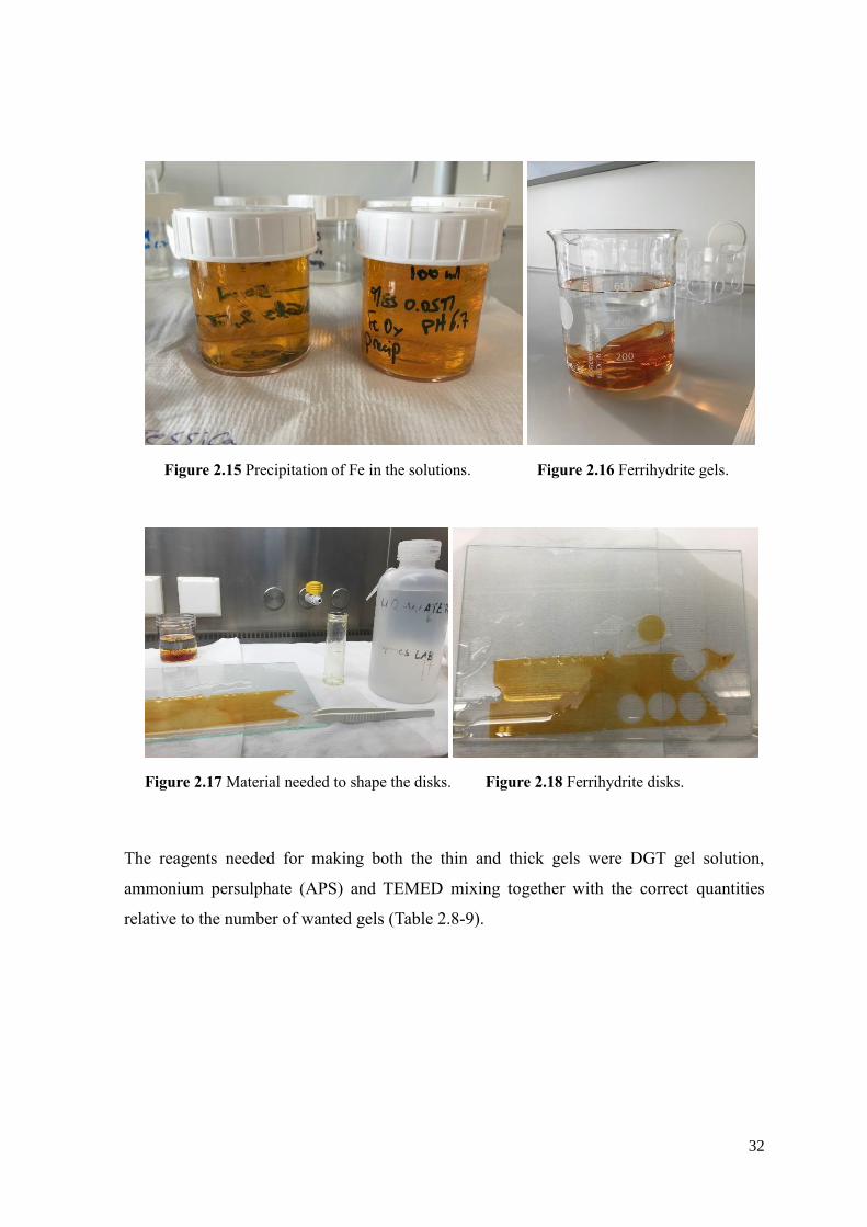
32

Figure 2.15 Precipitation of Fe in the solutions. Figure 2.16 Ferrihydrite gels.

Figure 2.17 Material needed to shape the disks. Figure 2.18 Ferrihydrite disks.

The reagents needed for making both the thin and thick gels were DGT gel solution,

ammonium persulphate (APS) and TEMED mixing together with the correct quantities

relative to the number of wanted gels (Table 2.8-9).

33

Thick diffusive gels (0.5 mm spacers, 0.8 mm hydrated gel):

# of gels

to be

prepared

Gel solution

(ml)

APS

(µl)

TEMED

(µl)

1 4 28 10

2 8 56 20

2.5 10 70 25

3 12 84 30

4 16 112 40

Table 2.8 Volume of solution and of reactants for thick diffusive gels.

Thin diffusive gels (0.25 mm spacers, 0.4 hydrated gel):

# of gels

to be

prepared

Gel solution

(ml)

APS

(µl)

TEMED

(µl)

1 2 14 5

2 4 28 10

3 6 42 15

4 8 56 20

5 10 70 25

Table 2.9 Volume of solution and of reactants for thin diffusive gels.

The gel solution was made by stirring 15 ml of DGT gel cross-linker with 47.5 ml of HQ

water in a beaker and with the successive addition of 37.5 ml of acrylamide solution. Once

the solution is prepared we used a 1 ml pipette, for the thin gels, and 5 ml pipette, for the

thick gels, to cast them inside the glass plates separated with Teflon spacers. For the 0.8 mm

thick diffusive gels were used 0.5 mm Teflon spacers and for the thin 0.25 mm thin diffusive

gels were used 0.25 mm Teflon spacers. During this action we paid attention to avoid a

possible formation of bubbles inside the gels that could decrease the available area; for this

reason, we used smooth plates freshly dried out of the acid bath. After casting the gel

between the glass plates, we placed them for 1 hour in the oven at 45°C for polymerization.

After opening the glass, we washed the polymerized gels in HQ water four times after two

34

hours each. When all the gels were ready we made disk with the same diameter of the DGT

plastic device.

Afterwards we close the DGT device with a front plate with an exposure window (A= 2.52

cm2): the pressure had to be equal in each direction to close it well and it had to avoid the

presence of air bubbles between the gel and/or membrane layers. Subsequently we stored

the assembled DGTs in a Ziploc-type PE bags with some water drops inside to maintain the

environment humid and we put them in the fridge until the moment of performing the

experiment.

.

Figure 2.19 The gels solution spreads left and

right by pipetting from the middle.

Figure 2.20 Some drops of water are

added on the top of the glass plate to see

better the gel.

Figure 2.21 DGTs ready and arranged in a plastic

bag in the fridge until the moment of the analysis

35

After 5 days of incubation (20 days in the other scenario) we removed the DGT from the

oven and we finished to assemble the DGT device adding a plexiglas frame, with a circle

hole of the same area, blocked with a screw on the side. Later, we put 5 g of dry soil, 10 g

on the safe side, on them filling completely the hole. Placing all DGTs in a box with a wet

tissue paper at the bottom, we incubated them at 20°C for an exposition time of 24h after the

application. A wet tissue paper was placed in the incubator in order to maintain a humid

atmosphere and avoid the drying of the soil. It is necessary to control the time of deployment

as closely as possible. To this effect, we recorded the paste application time and we removed

all the soil pastes before opening the DGTs at the end of experiment. The soil was removed

in a gentle way, in order not to move the 4 layers on the disks, and cleaned with a tissue

paper; later we took out the upper part of the devices and we discarded all the layers except

the ferrihydrated gel. We rinsed them with Millipore water, then we eluted the gels in 5 ml

of 0.25 M H2SO4; all the vials were left reacting on a plate shaker for the night.

Figure 2.22 DGTs device with plexiglas frame. Figure 2.23 DGTs device with soil on the top.

Figure 2.24 After 24 h the soil is removed

from the device.

Figure 2.25 Sample eluates on the plate

shaker.

36

The measurement of the eluates was done following the molybdenum blue method (in the

Appendix II): we used a HITACHI U-2000 Spectrophotometer at 881 nm.

The time-averaged concentration in the solution at the surface of the DGT device (𝐶𝐷𝐺𝑇) was

calculated using the Eq. (6):

𝑪𝑫𝑮𝑻 = 𝑀 ∗ ∆𝑔

𝐷 ∗ 𝐴 ∗ 𝑡 (𝟔)

Where ∆𝑔 is the thickness (cm) of the four diffusive layers, 𝐷(cm-2 s-1) the diffusion

coefficient of the analyte in the diffusive layer at the temperature of deployment (20°C), 𝐴

(cm2) the area of the exposure window, 𝑡 (s) the time of deployment and 𝑀 the resulting

mass of P in the eluant solution (Mason et al., 2008). The total amount of P in the volume of

eluate was calculated with the Eq. (7):

𝑴𝑫𝑮𝑻 = 𝐶 ∗ (𝑉𝐻2𝑆𝑂4+ 𝑉𝑖𝑟𝑜𝑛 𝑔𝑒𝑙) (𝟕)

Where 𝑉 is the sum of the volume of the H2SO4 and the volume of the iron gel and 𝐶 is the

P concentration obtained according to the calibration line and the dilution factor (in our case

equal to 1) and corrected for the blank values.

∆𝒈 (cm) 𝑫(cm-2 s-1) 𝑨(cm2) 𝒕(s) 𝑽𝑯𝟐𝑺𝑶𝟒+ 𝑽𝒊𝒓𝒐𝒏 𝒈𝒆𝒍 (ml)

0.095 0.00000527 3.14 86400 5.196

Table 2.10 The table contains the features of the diffusive layer, the time of deployment and the

volume of the eluate.

2.5. Pot trial

The experiment was performed with 51 pots: each fertilizer was replicated four times, except

for the Biogas Slurry (1 pot) and for Chicken Manure Biochar (2 pots) due to limited

fertilizer quantity. The weight of one pot was 33 g and we labelled them from 1 to 51: the

37

first four (from 1 to 4) were kept unfertilized as control. We put a piece of felt at the bottom

of with the plastic film at the top due to the water in the soil.

Figure 2.26 Pots labelled. Figure 2.27 Pot with felt cover at the bottom.

The first week we crushed the Melk soil clumps to smaller aggregates with a hammer and

sieved it with a 4 mm sieve.

Figure 2.28 Soil crushed with hamme. Figure 2.29 Sieve 4 mm.

We set up the pots with 1 kg of dry soil having 46.5% water holding capacity (WHC).

Fertilizer was added at the rate of 100 mgP kg-1 and mixed thoroughly. We added 284.25 ml

of water in order to reach 65% of maximum WHC, and. The final weight of one pot was

calculated as follows (8):

38

𝑻𝒐𝒕 𝒘𝒆𝒊𝒈𝒉𝒕𝒑𝒐𝒕 = 𝑤𝑒𝑖𝑔ℎ𝑡𝑒𝑚𝑝𝑡𝑦 𝑝𝑜𝑡 + 𝑤𝑎𝑡𝑒𝑟𝑎𝑑𝑑𝑒𝑑 + 𝑤𝑒𝑖𝑔ℎ𝑡𝑑𝑟𝑦 𝑠𝑜𝑖𝑙 + 𝑠𝑜𝑖𝑙 𝑚𝑜𝑖𝑠𝑡𝑢𝑟𝑒@ 𝑑𝑟𝑦 𝑎𝑖𝑟 =

= 33𝑔 + 284.25𝑔 + 1000𝑔 + 18𝑔 = 𝟏𝟑𝟑𝟓. 𝟐𝟓 𝒈 (8)

Each recycling fertilizer had its own features: different content of P for dry matter basis and

different water contents. Therefore, it was necessary to calculate the correct amount of

fertilizer to apply to the wet soil to have in each pot 100 mg P. Applying the following

formula (9):

𝒎𝒈 𝑷𝒇𝒆𝒓𝒕𝒊𝒍𝒊𝒛𝒆𝒓

𝒘𝒆𝒕 𝒔𝒐𝒊𝒍 ∗ 𝒑𝒐𝒕=

𝑚𝑔 𝑃𝑓𝑒𝑟𝑡𝑖𝑙𝑖𝑧𝑒𝑟

𝑝𝑜𝑡

(% 𝑃 100

∗1

𝑑𝑟𝑦 𝑚𝑎𝑡𝑡𝑒𝑟 𝑠𝑜𝑖𝑙∗

𝑑𝑟𝑦 𝑚𝑎𝑡𝑡𝑒𝑟 𝑠𝑜𝑖𝑙𝑤𝑒𝑡 𝑠𝑜𝑖𝑙

) (9)

We obtained those results:

# Pot Fertilizer

name

mg

P/kg

soil

added

kg soil

/pot mgP/pot

Fertilizer P

content (%

P DM basis)

Dry

Factor

mg

Fertilizer

/pot "wet"

weight

1 Blank 0 1 0 0 0 0

5 Bone meal 100 1 100 5.47 0.95 1928

9 CM 100 1 100 2.24 0.90 4933

13 Biogas Sl. 100 1 100 1.91 0.90 5802

14 BM BC 100 1 100 11.41 0.95 924

18 CM BC 100 1 100 4.37 0.98 2341

20 MSS BC 1 100 1 100 9.06 0.99 1117

24 MSS BC 2 100 1 100 6.88 0.88 1643

28 MSS A 1 100 1 100 7.95 0.98 1283

32 MSS A 2 100 1 100 10.41 0.99 971

36 Rock P. 100 1 100 14.29 1 700

40 SSP 100 1 100 9.50 1 1052

44 MAP 100 1 100 12.36 1 809

48 MSS BC 3 100 1 100 9.21 0.91 1197

Table 2.11 The table above contains the amount of fertilizer (mg) for pot needed to have 100 mgP

in one kg of soil.

We moved all the pots in a greenhouse with a temperature of 25°C.

39

The second week we planted 40 seeds of rye grass in every pot. We removed ~ 1,5 cm of the

upper part of the soil with a spoon and we scattered them and then we covered them softly

with the soil again.

Figure 2.30 Rye grass seeds.

We added water to maintain the weight around 1335 g and after 3 days we started to sprinkle

water every day to keep the soil moist and ease the sprouting and emergence. Giving your

seeds water on a regular basis to have the potting mixture always moist but never soaking.

Figure 2.31 Rye grass seeds spread around the surface of the pot.

The light is an integral component to plant photosynthesis, which is the metabolic process

necessary for plants to grow and flourish: the light and the heat were provided by lamps. To

manage this was measured the amount of light the plants were receiving and tried to match

it to its optimal light intensity. Therefore, we monitored it in 4 different points (the left and

right side and 2 check-point in the middle of the table) at the same height corresponding the

40

possible max height reached by the plants. We used a photosynthetically active radiation

(PAR) meter every 5 days:

date of

measurement

point #1

(close to

the

window)

point #2

(in the middle

(close to the

window))

point #3

(in the

middle

(close to the

door))

point #4

(close to

the door)

weather

condition

11/feb/2016 1289 µm 690 µm 590 µm 630 µm Sunny

18/feb/2016 590 µm 526 µm 620 µm 615 µm cloudy

23/feb/2016 570 µm 630 µm 595 µm 629 µm cloudy

01/mar/2016 570 µm 620 µm 460 µm 530 µm cloudy

08/mar/2016 558 µm 620 µm 486 µm 536 µm cloudy

Table 2.12 Light density received by the photosynthetically active radiation in 5 different days.

After one week (third week) the plants were thinned to 25 per pot, cutting the amount in

excess with a scissor. At the beginning we controlled the number frequently, after a week

we checked them twice a week.

Figure 2.32 seeds begin to push tiny sprouts through the soil.

In the same week we added 50 ml of P free solution for non-leguminous plants (modified

from Middleton & Toxopeus 1973) to each of the 51 pots. This fertilization was done once

a week, i.e. 5 times until the harvest.

41

It was 2.5 l of solution composed of (1) 500 ml macronutrient stock solution, (2) 500 ml

micronutrient stock solution, (3) 500 ml Fe EDDHA stock solution, and deionized water to

bring to final volume. Thus each stock solution was diluted 1:5.

The stock solutions of macronutrients, micronutrients and FeEDDHA were prepared as

follows:

(1) MACRONUTRIENTS STOCK (g/l)

NH4NO3 17

K2SO4, anhydr. 7.35

MgSO4 7H2O 2.22

CaCO3, anhydr 1.8

HCl, N (= 1 Molar) 36 ml

NaCl 0

(2) MICRONUTRIENTS STOCK (mg/l)

H3BO3 (a) 3

CuCl2 (b) 0.8

MnCl2 4H2O 27.5

(NH4)Mo7O24 4H2O (c) 0.4

ZnCl2 (d) 1.5

(a) Dissolve 30mg H3BO3 in100ml (=300mg/l)

(b) Dissolve 20mg CuCl2 in 250ml(=80mg/l)

(c) Dissolve 10mg Ammonium heptamolybdate in 250ml(=40mg/l)

(d) Dissolve 15mg ZnCl2 in 100ml(=150mg/l)

The amount of B, Cu, Mo and Zn were very little and difficult to measure and so it

was better to prepare concentrated solution first and later add 10ml of each a, b, c,

and d solution in 1l micronutrient stock solution, or 20ml in 2l (Dilution Factor

=100).

(3) Fe EDDHA stock 12mg/l

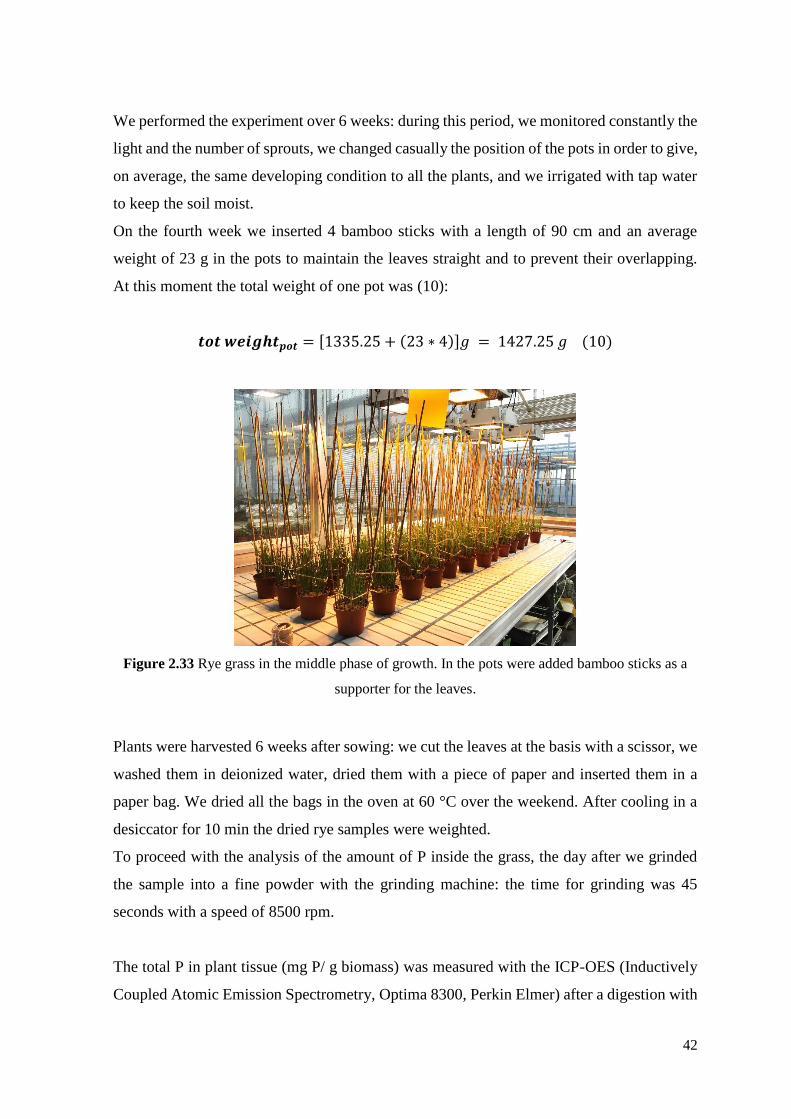
42

We performed the experiment over 6 weeks: during this period, we monitored constantly the

light and the number of sprouts, we changed casually the position of the pots in order to give,

on average, the same developing condition to all the plants, and we irrigated with tap water

to keep the soil moist.

On the fourth week we inserted 4 bamboo sticks with a length of 90 cm and an average

weight of 23 g in the pots to maintain the leaves straight and to prevent their overlapping.

At this moment the total weight of one pot was (10):

𝒕𝒐𝒕 𝒘𝒆𝒊𝒈𝒉𝒕𝒑𝒐𝒕 = [1335.25 + (23 ∗ 4)]𝑔 = 1427.25 𝑔 (10)

Figure 2.33 Rye grass in the middle phase of growth. In the pots were added bamboo sticks as a

supporter for the leaves.

Plants were harvested 6 weeks after sowing: we cut the leaves at the basis with a scissor, we

washed them in deionized water, dried them with a piece of paper and inserted them in a

paper bag. We dried all the bags in the oven at 60 °C over the weekend. After cooling in a

desiccator for 10 min the dried rye samples were weighted.

To proceed with the analysis of the amount of P inside the grass, the day after we grinded

the sample into a fine powder with the grinding machine: the time for grinding was 45

seconds with a speed of 8500 rpm.

The total P in plant tissue (mg P/ g biomass) was measured with the ICP-OES (Inductively

Coupled Atomic Emission Spectrometry, Optima 8300, Perkin Elmer) after a digestion with

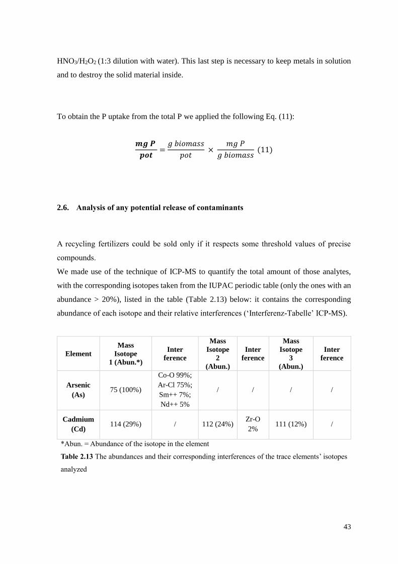
43

HNO3/H2O2 (1:3 dilution with water). This last step is necessary to keep metals in solution

and to destroy the solid material inside.

To obtain the P uptake from the total P we applied the following Eq. (11):

𝒎𝒈 𝑷

𝒑𝒐𝒕=

𝑔 𝑏𝑖𝑜𝑚𝑎𝑠𝑠

𝑝𝑜𝑡 ×

𝑚𝑔 𝑃

𝑔 𝑏𝑖𝑜𝑚𝑎𝑠𝑠 (11)

2.6. Analysis of any potential release of contaminants

A recycling fertilizers could be sold only if it respects some threshold values of precise

compounds.

We made use of the technique of ICP-MS to quantify the total amount of those analytes,

with the corresponding isotopes taken from the IUPAC periodic table (only the ones with an

abundance > 20%), listed in the table (Table 2.13) below: it contains the corresponding

abundance of each isotope and their relative interferences (‘Interferenz-Tabelle’ ICP-MS).

Element

Mass

Isotope

1 (Abun.*)

Inter

ference

Mass

Isotope

2

(Abun.)

Inter

ference

Mass

Isotope

3

(Abun.)

Inter

ference

Arsenic

(As) 75 (100%)

Co-O 99%;

Ar-Cl 75%;

Sm++ 7%;

Nd++ 5%

/ / / /

Cadmium

(Cd) 114 (29%) / 112 (24%)

Zr-O

2% 111 (12%) /

*Abun. = Abundance of the isotope in the element


analyzed

44

Element

Mass

Isotope

1 (Abun.*)

Inter

ference

Mass

Isotope

2

(Abun.)

Inter

ference

Mass

Isotope

3

(Abun.)

Inter

ference

Chromium

(Cr) 52 (84%)

Pd ++ 9%,

Ru++ 18%;

Ar-C 98%;

Cl-O-H 75%

/ / / /

Copper

(Cu) 63 (70%)

Ti-O 7%;

Te++ 19%;

Ar-Na 99%;

Ti-O-H 8%;

P-O-O 99%

65

(30.83%)

Ti-O

5%; Ar-

Mg

10%;

Te++

35%;

Xe++

4%; Ti-

O-H

74%

/ /

Nickel (Ni) 58 (68%) Na-Cl 75% 60 (26%) Na-Cl

24% / /

Lead (Pb) 208 (52%) Os-O 40% 206 (24%) Os-O

26% / /

Vanadium

(V) 51 (99%)

Ru++ 31%,

Cl-O 75%,

Cl-N 24%

Ar-B 80%

/ / 207 (22%) Ir-O 38%

Zinc (Zn) 64 (48%)

Ti-O 73%,

S-S 90%,

Ar-Mg 78%,

Te++ 31%,

S-O-O 94%

66 (28%) Ar-Mg

11% 68 (19%)

Cr-O

84%; Ar-

Si 91%;

Iron (Fe) 57 (2%)

Cd++ 28%;

K-O 6%; Ar-

O-H 99%

56 (92%)

Cd++

23%;

Ar-O

99%;

Ca-O

96%

/ /

*Abun. = Abundance of the isotope in the element


analyzed.

45

Figure 2.34 ICP-MS (Perkin Elmer)

2.6.1. Preparation of the samples and the standards

First of all, the samples were digested by two different reagents: Aqua Regia (AR), for the

range of recycling fertilizers including mineral conventional fertilizers, animal manures,

municipal sewage sludge and their respective biochars and HNO3-H2O2, for the samples with

high organic matter content like feedstocks.

The procedures were:

- Aqua Regia (AR) Digestion: firstly, it is necessary weigh 100 mg of each fertilizer

in the digestion tube (for microwave or for digestion block) and add 1.5 ml 65%

HNO3 and 4.5 ml 37% HCl directly to the tube. Once it is done it is possible to

perform the digestion program for soil in the microwave digester Anton Paar -

Multiwave 3000. After the digestion the tube is rinsed and all the samples are

transferred into a 100 ml vial (pre-weighted without cap) bringing the volume to ca

75 ml with HQ (deionized) water (staying below 80 ml). On a scale the sample weight

is brought to 83.25 g (total weight = vial weight + 83.25g) in order to dilute the

sample so as to contain 4% acid (HCl + HNO3). After stirring the mixture to ensure

a homogenous concentration of the elements, the aliquote was filter through a filter

papers with a plastic funnel into a 50 ml vial.

Figure 2.35 samples got in the position for the

analysis.

35)

46

Figure 2.36 Digestion tubes and acids, Figure 2.37 Ceramic digestion tubes with lids and sensor,

Figure 2.38 Microwave digester Anton Paar - Multiwave 3000.

- Digestion with HNO3 + H2O2: it is weight 100 mg of each fertilizer in a digestion

tube for microwave and it is added 5 ml 65% HNO3 and 1 ml H2O2 . Later on it is

performed the program for plant digestion in the microwave. Once the digestion

process is finished the tubes are rinsed and the whole digestated is moved into 100

ml vial (pre-weighed without cap). Adding water, the volume is firstly brought to ca

70 ml, staying below 75 ml, and after the sample is weighed on a scale to reach 75.33

g (total weight=vial weight + 75.33g). In this way the sample contains 6% acid (HCl

+ HNO3) and it has a density of 1.032 with a volume of 72.99 ml. The mixture is

stirred to ensure homogenous concentration of elements and then it is filter with

funnel and paper filter into a 50 ml vial.

All the samples were replicated three times and then they were diluted 1:20 with 2% HNO3.

Figure 2.39 Sample digested: the yellow one corresponding to the AR digestion, the one

corresponding to the HNO3 + H2O2 digestion.

38)

36)

37)

47

Subsequently we prepared:

- The standards for the calibration required to construct a multipoint standard curve

covering the range of analyte concentration;

- The Quality Control standards necessary to check if the measure made by the

machine is done always in the same conditions;

- The QM essential to control the measure of the elements inside the not diluted

solutions.

2.6.2. Instrumental setting and calibration

Prior to sample analysis we set up the instrument to monitor isotopes of the compounds

selected (Table 2.13) and the gas mode (Indium, In).

Analysing the calibration standards and using the linear regression analysis, the software

automatically plotted the relative response vs. the concentration in ng/l and determine slope

(m), intercept (b), and correlation coefficient (ρ).

This can be automatically performed by the ICP-MS software. Correlation coefficient ρ must

be as high as possible: ≥0.995 is generally obtained for standards that are well prepared.

2.6.3. Injection sequence and calculations

Calibration blanks and QC standards must be included in the sample analysis sequence to

verify instrument performance over the course of the run. If the response of any sample

exceeds highest standard in the calibration curve an appropriate dilution has to be made.

The instrument software was programmed to perform all necessary calculations. It used the

values for m, b determined for the calibration curve to quantify the selected analyte

concentration (𝐶𝑒𝑥𝑡𝑟𝑎𝑐𝑡, in µg/l) in any extract having a relative response R using the Eq.

(12):

48

𝑪𝒆𝒙𝒕𝒓𝒂𝒄𝒕 = 𝑅 − 𝑏

𝑚 (12)

Because of the measure of the analytes was done with analytical technique, we firstly

calculated the limit of detection (LOD) and the limit of quantification (LOQ) to verify the

suitability of the results by the ICP-MS. They were evaluated applying the equations (13)

and (14) of the method ‘blank determination’:

𝑳𝑶𝑫 = 𝑚𝑒𝑎𝑛𝑏𝑙𝑎𝑛𝑘𝑠 + 3 ∗ 𝑆𝐷𝐵𝐿𝐴𝑁𝐾𝑆 (13)

𝑳𝑶𝑸 = 𝑚𝑒𝑎𝑛𝑏𝑙𝑎𝑛𝑘𝑠 + 10 ∗ 𝑆𝐷𝐵𝐿𝐴𝑁𝐾𝑆 (14)

Figure 2.40 Illustration of the concept of detection and quantification limit by showing the

theoretical normal distributions associated with blank, detection limit and quantification limit level

samples. LOD is defined as 3 * standard deviation of the blank, and at the LOQ defined as 10 *

standard deviation of the blank. For a signal at the LOD, the alpha error (probability of false positive)

is small (1%). However, the beta error (probability of a false negative) is 50% for a sample that has

a concentration at the LOD (red line). This means a sample could contain an impurity at the LOD,

but there is a 50% chance that a measurement would give a result less than the LOD. At the LOQ

(blue line), there is minimal chance of a false negative.

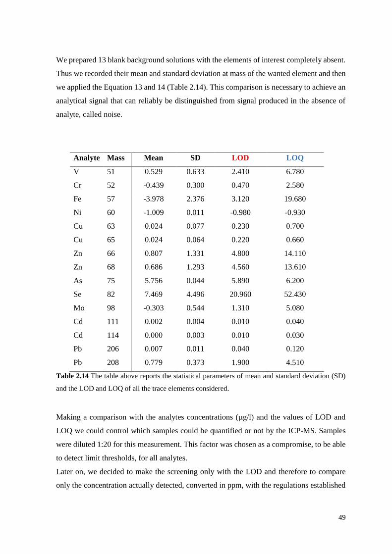
49

We prepared 13 blank background solutions with the elements of interest completely absent.

Thus we recorded their mean and standard deviation at mass of the wanted element and then

we applied the Equation 13 and 14 (Table 2.14). This comparison is necessary to achieve an

analytical signal that can reliably be distinguished from signal produced in the absence of

analyte, called noise.

Analyte Mass Mean SD LOD LOQ

V 51 0.529 0.633 2.410 6.780

Cr 52 -0.439 0.300 0.470 2.580

Fe 57 -3.978 2.376 3.120 19.680

Ni 60 -1.009 0.011 -0.980 -0.930

Cu 63 0.024 0.077 0.230 0.700

Cu 65 0.024 0.064 0.220 0.660

Zn 66 0.807 1.331 4.800 14.110

Zn 68 0.686 1.293 4.560 13.610

As 75 5.756 0.044 5.890 6.200

Se 82 7.469 4.496 20.960 52.430

Mo 98 -0.303 0.544 1.310 5.080

Cd 111 0.002 0.004 0.010 0.040

Cd 114 0.000 0.003 0.010 0.030

Pb 206 0.007 0.011 0.040 0.120

Pb 208 0.779 0.373 1.900 4.510

Table 2.14 The table above reports the statistical parameters of mean and standard deviation (SD)

and the LOD and LOQ of all the trace elements considered.

Making a comparison with the analytes concentrations (µg/l) and the values of LOD and

LOQ we could control which samples could be quantified or not by the ICP-MS. Samples

were diluted 1:20 for this measurement. This factor was chosen as a compromise, to be able

to detect limit thresholds, for all analytes.

Later on, we decided to make the screening only with the LOD and therefore to compare

only the concentration actually detected, converted in ppm, with the regulations established

50

for contaminants in fertilizers (Table 2.15) in order to establish if the thirteen recycling

fertilizers can be sold as environmental safe product on market. By this evaluation we

observed that for the Lead isotope of mass 208 all the values, both with the AR and HNO3 –

H2O2 digestion, were below the LOD; thus it was not further examined. Regarding Arsenic,

Cadmium, Chromium, Zinc and Vanadium, they present few values, scattered in both

digestions, lower than the limit; instead Lead (isotope of mass 206), Copper, Nickel and Iron

had detectable amounts in all samples

From this we wanted to obtain the concentration of the elements (𝐶𝑠𝑜𝑖𝑙) in respect to the

weight of dry soil (mganalyte/kgdrysoil, ppm) applying the following Eq. (15):

𝑪𝒔𝒐𝒊𝒍 =𝐶𝑒𝑥𝑡𝑟𝑎𝑐𝑡

1000× 𝐷𝐹 × 𝑉𝑒𝑥𝑡𝑟𝑎𝑐𝑡𝑖𝑜𝑛 ×

1

𝑤𝑒𝑖𝑔ℎ𝑡𝑠𝑎𝑚𝑝𝑙𝑒 × 𝐷𝑟𝑦𝐹𝑎𝑐𝑡𝑜𝑟 (15)

Where 𝐷𝐹 is the dilution factor and 𝑉𝑒𝑥𝑡𝑟𝑎𝑐𝑡𝑖𝑜𝑛 is the volume of the extract for the AR and

HNO3 + H2O2 digestions (l). The 𝑤𝑒𝑖𝑔ℎ𝑡𝑠𝑎𝑚𝑝𝑙𝑒 in kg times the 𝐷𝑟𝑦𝐹𝑎𝑐𝑡𝑜𝑟 give the dry

weight of the sample.

REFERENCE Feedstock Pb

ppm

Zn

ppm

Cd

ppm

Cr

ppm

Cu

ppm

Ni

ppm

As

ppm

V

ppm

Threshold Basic

deutschen

Bundes-

Bodenschutzver

ordnung

(BBodSchV)

(EBC)

BC 150 400 1.5 90 100 50 40 /

EC 86/278/EEC

High MSS 1200 / 40 / 1750 400 / /

EC 86/278/EEC

Low MSS 750 2000 20 / 1000 300 / /

*RF= recycled fertilizer; **SOW= Stabilized Organic Waste.



expressed in mgelement/kgsoil or mgelement/kgP2O5

51

REFERENCE Feedstock Pb

ppm

Zn

ppm

Cd

ppm

Cr

ppm

Cu

ppm

Ni

ppm

As

ppm

V

ppm

EU Draft

Directive 2015 MSS 500 2000 5 800 800 200 / /

DE Regulation RF* 150 / 1.5 / / 80 / /

CH Regulation RF 120 400 1 2000 100 30 / /

EC 2001 2nd

Working

document

SOW** 500 1500 5 600 600 150 / /

Düngemittelvero

rdnung 2004

(Austrian

Fertilitzer

Regulation)

DüMit>5

% P2O5

100

mg

Pb/k

gP2

O5

/

75

mg

Cd/k

gP2

O5

/ /

100

mg

Ni/k

gP2

O5

40

mg

As/k

gP2

O5

1500

mg

V/kg

P2O5

Compost

ordinance 2001

(BGBL.II

292/2001)

Class A+

Compost 45 200 0.7 70 70 25 / /

Compost

ordinance 2001

(BGBL.II

292/2001)

Class A

Compost 120 500 1 70 150 60 / /

Compost

ordinance 2001

(BGBL.II

292/2001)

Class B

Compost 200 1800 3 250 500 100 / /

*RF= recycled fertilizer; **SOW= Stabilized Organic Waste.



expressed in mgelement/kgsoil or mgelement/kgP2O5

From the table above, it is possible to notice that not the entire group of the decided element

are under regulation; the main reason is the fact that some elements, as iron, zinc and copper,

are considered micro-nutrients for the plants.

52

2.7. Statistics

Statistical analysis was performed by Microsoft Excel 2010 (Microsoft corporation). In this

research the following statistical parameters were taken into account: the standard deviation

(SD) and the derived coefficient of variation (CV), the mean value (∆), the Pearson value

(ρ), the R-squared (R2), the p-value and the behaviour of the errors (ɛ). We used the

coefficient of variation (CV) (CV=SD/mean*100) in order to assess the variability of the

results. The smaller the CV, the lower is the variability due to random experimental factors.

The ρ, R2 and ɛ were employed to evaluate a possible linear correlation between the data

series.

The number of the samples was 13, considering the mean value of the replicates.

53

3. RESULTS

3.1. Calcium Acetate Calcium Lactate (CAL)

The graph below shows that the majority of CAL values ranges from 20-60 mg P/ kg_ dry

soil, except for the response corresponding to biogas-slurry fertilization that exceeds 120 mg

P/kg and for the Rock P and MSS BC 3 that are below the lowest value. Therefore, from this

data we cannot say that treatments as pyrolysis or gasification raise more P for plants.

All the values are greater than the control soil (~13 mg/kg) with the exception of the MSS

BC, Rock P and MSS BC 3.

Figure 3.1 P extracted from soil sample fertilized by 13 amendments with the CAL method. The

amount is expressed in mgP/kg DM and it is the mean value of experimental replicates (n=3). Error

bars indicate standard deviation of them.

0

20

40

60

80

100

120

140

160

P e

xtr

act

ed (

mg P

/kg)

type of fertilizer

CAL results

54

By the evaluation of the coefficient of variation in %, only the cases of MSS BC 2 and MSS

A 1 have > 10%; therefore, it is possible to declare that we do not have a large dispersion of

the data evaluated.

3.2. Olsen method

The following graph depicts the P extracted using the Olsen method that estimates the

sodium-bicarbonate extractable phosphorus.

Olsen P values obtained from the 13 fertilizers studied ranged from 9.4 to 83.9 mg P/kg,

with the minimum corresponding to Bone meal (moreover below to the blank samples that

has a mean value of 10 mg P/kg) and the maximum was MAP.

The values are quite low and they are around 10-20 mgP/kg with the exception of MAP and

SSP that are higher but with a larger coefficient of variation (>10%). The biochars obtained

by pyrolysis do not show a huge increase of P availability in comparison with their feedstock,

furthermore the P measured by the bone meal BC is lower than that of the bone meal.

All the extractions give a larger P extracted than the control sample, apart from the bone

meal sample (9.4 < 10 mg P/kg).

55

Figure 3.2 Extractable soil P fraction from soil sample fertilized by 13 amendments with the CAL

method. The amount is expressed in mg P/kg DM and the first bar (brighter colour) belongs to the

control sample. The values are the average of experimental replicates (n=3) and the error bars indicate

standard deviation of them.

With regard to the accuracy of the data, only the MAP extraction has a coefficient of

variation higher than 10%.

3.3. Diffusive Gradient in Thin Films

The figure 3.3 shows the CDGT results after 5 days of incubation and after 20 days of

incubation.

0

20

40

60

80

100

120

P e

xtr

act

ed (

mg

P/k

g)

type of fertilizer

Olsen results

56

Figure 3.3 DGT measurements (µgP l-1) on the gel for one type of soil fertilized with 13 type of

fertilizers. The two series of data are related to the two different incubation of time. The two bars in

brighter color belong to the control sample. Error bars indicate the standard deviation of experimental

replicates (n=3).

As can be seen, the DGT method produced values for available P of 12.5 µg/l to 168.5 µg/l

(5 days’ case) and of 13.5 µg/l to 179.5 µg/l (20 days’ case). The fertilizer that achieve the

highest amount of P, in both cases of study, are MAP, SSP, chicken manure and its BC and

biogas slurry. The other were below 50 µg/l and not always greater than the blank sample

(14.4 µg/l for 5 days and 13.8 µg/l for 20 days). From this representation the mixture with

BC do not increase the value of CDGT in comparison with their feedstock, except for the case

of chicken manure BC.

Comparing the data after 5 and 20 days of incubation, we can observe that there is not a fixed

trend of the P uptake: fertilizers as Bone meal and its BC, Biogas slurry, MSS BC, MSS BC

2 and SSP raise more P after the first incubation, on the other hand chicken manure, bone

meal BC, MSS A 1, MSS A 2, Rock P, MAP and MSS BC 3 achieve a higher amount after

20 days. There is not such a large diversity between the results obtained in the two period of

incubation, except for the samples of chicken manure BC, SSP and MAP (Table 3.1).

0

50

100

150

200

250C

DG

T(µ

gP

l-1

)

type of fertilizer

DGT results

5 days

20 days

57

Chicken manure BC SSP MAP

P5d P20d P5d P20d P5d P20d

139 µg/l 109.9 µg/l 168.5µg/l 115.4µg/l 134.4µg/l 179.5µg/l

Table 3.1 Concentration of P measured with DGT for the CMBC, SSP and MAP samples in the two

different period of incubation.

About a statistical analysis, 4 out of 13 fertilizers’ 5 days’ incubation data have a CV higher

than 10%, therefore the data are not too much dispersed around the mean value. In the other

case, 9 out of 13 have a high CV which shows larger experimental.

3.4. Plant growth

The graph (Figure 3.4) below shows the weight of the biomass growth by the adding of 100

mg P/ kg soil with the 13 type of fertilizers studied. With this representation we have the

possibility to understand which amendment released more available P. Furthermore, we can

also observe the difference between the growth of the ryegrass with and without the

fertilization, making a comparison between the data of the fertilized soil and the blank

sample.

58

Figure 3.4 Biomass weight for each type of fertilizer and for the control sample. The control sample

has a brighter colour to underline the difference between the other. Error bars are the standard

deviation of experimental samples (n=3).

It is detectable that all the values are greater than the one reached by the soil without

fertilization, indicating that every category of amendment lead an increase of biomass. In

most cases the values are between 4 and 5 g, except for 6 out of the 13 fertilizers that are

outside of the range (Bone meal, Chicken Manure, Biogas slurry, Chicken manure BC, SSP,

MAP).

All the measurements don’t show a high coefficient of variation (the highest ~ 12%),

therefore we can affirm that they are reliable.

The biomass was later analysed with the spectrometry technique of the ICP-OES to reveal

the quantity of P picked up by the plant from the soil in the pot (mg P/g).

0

1

2

3

4

5

6

7

8

Bio

ma

ss g

row

th (

g)

type of fertilizer

Avarage value of aboveground biomass

59

Figure 3.5 The histogram shows the P up taking by the plant in the 13 cases in which the soil was

fertilized with diverse fertilize; it is also shown the control amount (in a lighter colour) to catch better

an increase of the uptaking. The harvest was done after 6 weeks of growth. The values are the mean

between three experimental samples (n=3) and the error bars represent the standard deviation of

them.

About the standard deviation, four samples out 13 have CV > 10%.

3.5. Correlation between the pot trial and the soil P test

As we said before, a possible solution to the problem of lack of P for agricultures the

recycling / recovery of it from various waste flows. It is required to use accurate methods to

test P availability from these new fertilizers.

In this thesis we studied the accuracy of two standard methods (CAL, Olsen) and a novel

soil test (DGT): to evaluate their prediction of plant P availability we fit the plant P uptake

with the results given by the tests. The pot trial being the most reliable test, if the correlation

between the two data series has a high R2 value, it is possible to affirm that the soil P test

gives a good prediction of P availability.

0

5

10

15

20

25

P u

ptk

ae

(mg

P/p

ot)

type of fertilizers

Plant P uptake

60

The graphs below show the correlation between the pot trial and the soil P test results (Figure

3.6, 7, 8, 9).

The four graphs show the possible linear correlation between the plant P uptake measured with the

ICP-OES (mgP/pot) at increasing of: Figure 3.6 detected P with DGT device in 5 days (µgP/l),

Figure 3.7 detected P with DGT device in 20 days (µgP/l), Figure 3.8 extractable soil P (mgP/kg)

revealed by Olsen method with 5 days of incubation, Figure 3.9 extractable soil P (mgP/kg) revealed

by CAL method with 5 days of incubation. The calibration line, with its corresponding parameter R2,

was calculated with Excel.

R² = 0,88

0

5

10

15

20

25

0 50 100 150 200

Pla

nt

P u

pta

ke

(mgP

/ p

ot)

C DGT_5 (µg/l)

Plant P uptake vs CDGT_5

R² = 0,94

0

5

10

15

20

25

0 50 100 150 200

Pla

nt

P u

pta

ke

(mgP

/ p

ot)

C DGT 20 (µg/l)

Plant P uptake vs CDGT_20

R² = 0,88

0

5

10

15

20

25

0 20 40 60 80 100

Pla

nt

P u

pta

ke

(mgP

/ p

ot)

Olsen 5 days (mg P/kg)

Plant P uptake vs Olsen results

R² = 0,16

0

5

10

15

20

25

0 20 40 60 80 100 120 140

Pla

nt

P u

pta

ke

(mgP

/ p

ot)

CAL 5 days (mg P/kg)

Plant P uptake vs CAL results

6) 7)

9) 8)

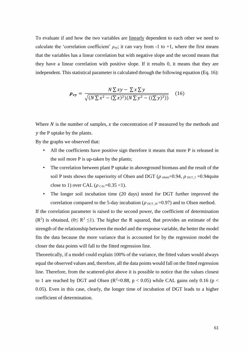
61

To evaluate if and how the two variables are linearly dependent to each other we need to

calculate the ‘correlation coefficient’ ρxy; it can vary from -1 to +1, where the first means

that the variables has a linear correlation but with negative slope and the second means that

they have a linear correlation with positive slope. If it results 0, it means that they are

independent. This statistical parameter is calculated through the following equation (Eq. 16):

𝝆𝒙𝒚 = 𝑁 ∑ 𝑥𝑦 − ∑ 𝑥 ∑ 𝑦

√(𝑁 ∑ 𝑥2 − (∑ 𝑥)2)(𝑁 ∑ 𝑦2 − ((∑ 𝑦)2)) (16)

Where 𝑁 is the number of samples, 𝑥 the concentration of P measured by the methods and

𝑦 the P uptake by the plants.

By the graphs we observed that:

• All the coefficients have positive sign therefore it means that more P is released in

the soil more P is up-taken by the plants;

• The correlation between plant P uptake in aboveground biomass and the result of the

soil P tests shows the superiority of Olsen and DGT (𝜌 olsen=0.94, 𝜌 DGT_5 =0.94quite

close to 1) over CAL (𝜌 CAL=0.35 <1).

• The longer soil incubation time (20 days) tested for DGT further improved the

correlation compared to the 5-day incubation (𝜌 DGT_20 =0.97) and to Olsen method.

If the correlation parameter is raised to the second power, the coefficient of determination

(R2) is obtained, (0≤ R2 ≤1). The higher the R squared, that provides an estimate of the

strength of the relationship between the model and the response variable, the better the model

fits the data because the more variance that is accounted for by the regression model the

closer the data points will fall to the fitted regression line.

Theoretically, if a model could explain 100% of the variance, the fitted values would always

equal the observed values and, therefore, all the data points would fall on the fitted regression

line. Therefore, from the scattered-plot above it is possible to notice that the values closest

to 1 are reached by DGT and Olsen (R2=0.88, p < 0.05) while CAL gains only 0.16 (p <

0.05). Even in this case, clearly, the longer time of incubation of DGT leads to a higher

coefficient of determination.

62

Those numerical observations are figured well by the graphs: we can see that in the case of

Olsen and DGT the points are more close to the prediction line, instead in the CAL method

the sample points are more scattered in the area.

Those coefficients show the being of a correlation between the two variables but they do not

prove the causality of the correlation. A best way to verify if this assumption is true is to

check the dispersion of the residual errors (ɛ = Y – Ŷ, where Y is the measured value and Ŷ

is the value calculated with the line, obtaining by the least squares, that fit better the

dispersion of the data) with a dispersion graph.

First of all, it was calculating the equation line for each method, Ŷ= b0 + b1x (by the statistical

tools of the Excel program) that are reported in the table below.

Method b0 b1

DGT5 2.866 0.093

DGT20 2.560 0.010

Olsen 2.380 0.230

CAL 4.680 0.070

Table 3.2 List of the intercept (b0) and the angular coefficient (b1) for the lines estimated by the

statistical tools of Excel, regarding all the chemical methods analysed in this research

63

Then we plotted the Ŷ versus ɛ:

The diagrams plot the estimated value Ŷ by the correlation line with the residue ɛ for each method

used: Figure 3.10 DGT with 5 days of soil incubation, Figure 3.11 DGT in 20 days of soil

incubation, Figure 3.12 Olsen method and Figure 3.13 CAL method.

-10

-8

-6

-4

-2

0

2

4

6

8

10

0 5 10 15 20

ɛ

Ŷ

CDGT_5

-10

-8

-6

-4

-2

0

2

4

6

8

10

0 10 20 30

ɛ

Ŷ

CDGT_20

-10

-8

-6

-4

-2

0

2

4

6

8

10

0 10 20 30

ɛ

Ŷ

Olsen

-10

-8

-6

-4

-2

0

2

4

6

8

10

0 5 10 15

ɛ

Ŷ

CAL

10) 11)

13) 12)

64

And we plotted x versus ɛ:

The diagrams plot the predictor x with the residue ɛ for each method used: Figure 3.14 DGT with 5

days of soil incubation, Figure 3.15 DGT in 20 days of soil incubation, Figure 3.16 Olsen method

and Figure 3.17 CAL method.

In all the diagrams we can see that all the data are quite good spread out the zero with the

meaning that the model for the linear regression that we had adopted it is good to describe

the relation between the x and Ŷ. The DGT results are the closest to the zero value. The

worst trend is represented by CAL because the data get far with the increasing of the Ŷ and

x. This shape suggests that the linear model doesn’t fit well the existing relation between the

variables.

-10

-8

-6

-4

-2

0

2

4

6

8

10

0 50 100 150 200

ɛ

x

CDGT_5

-10

-8

-6

-4

-2

0

2

4

6

8

10

0 50 100 150 200

ɛ

x

CDGT_20

-10

-8

-6

-4

-2

0

2

4

6

8

10

0 50 100

ɛ

x

Olsen

-10

-8

-6

-4

-2

0

2

4

6

8

10

0 50 100 150

ɛ

x

CAL

14)

16) 17)

15)

65

Besides, it is possible to observe that in the graphs with more reliability, there are six/seven

points concentrated around 5 mgP/pot at the beginning of the prediction line, while the other

are more detached and distinguished. The fertilizers which have less P availability are MSS

BC 1, Bone meal and its BC, MSS BC 2, MSS A 1, MSS A 2, Rock P and MSS BC 3.

Therefore, we can notice that the biochars, with the exception of chicken manure BC, do not

release a large quantity of P available for the plant up-taking.

3.6.Analysis of the possible contaminations of the recycling fertilizers

The bar-plots below report the comparison between the trace elements’ concentrations

(mgelement/kg or mgelement/kgP2O5) in the recycled fertilizer.

As can be seen, the concentrations measured with the two different types of digestion show

similar results in the most cases. I chose to not represent the value of Iron because there are

not thresholds established in all the regulations analyzed.

In all the graphs I marked the limit quantities decided by the European legislation in order

to make more visible a possible excess.

66

Vanadium


are the concentration of V by the Aqua Regia digestion, instead the bars in brighter grey are the

concentration of V by HNO3-H2O2. All the values are expressed in mgV/ kgP2O5. The Error bars

represent the standard deviation of experimental samples (n=3).

The unique legislations for V is the Düngemittelverordnung 2004 that sets up 1500

mgV/kgP2O5 as limit for the amendments containing more than 5% of P2O5. It is possible to

notice that the maximum value is reached by the SSP but it is very far from the threshold.

0

100

200

300

400

500

600

700

800

Co

ncen

tra

tio

n o

f V

(m

gV

/ k

gP

2O

5)

V

AR HNO3-H2O2

67

Chromium


are the concentration of Cr by the Aqua Regia digestion, instead the bars in brighter grey are the

concentration of Cr by HNO3-H2O2. All the values are expressed in mgCr/ kg. The Error bars


amount of the compost regulation and the yellow line means the threshold value of the EBC

regulation.

Regarding the BC, we can notice that the MSS BC 2/3 exceed the threshold of 90 ppm Cr

(EBC legislation, yellow line). The compost ordinance 2001 (class B, A, A+, blue lines) is

not respected in several fertilizers: MSS A 1 goes lightly beyond the 250 ppm (class B),

whereas all the BCs, the ashes from the MSS and the Rock P are not good for the class A,

A+ and B. It is good to underline that the Swiss regulation for the recycled fertilizers is

abided by (2000 ppm).

-40

-20

0

20

40

60

80

100

120

140

160

180

200

220

240

260

280

Co

nce

ntr

ati

on

Cr (

pp

m)

Cr

AR HNO3-H2O2

68

Nickel


are the concentration of Ni by the Aqua Regia digestion, instead the bars in brighter grey are the

concentration of Ni by HNO3-H2O2. All the values are expressed in mgNi/ kg. The Error bars


amount of the compost regulation, the red line is for the German Legislation and the green one is for

the Swiss one.

The two ashes are not in compliance with the compost ordinance, for all the three classes

(blue lines) and with both the German (red line) and Swiss regulation (green line). The

residues from MSS, both BC and ashes, could not be used according to the German, the

Swiss and the Düngemittelverordnung (100 mg Ni/kgP2O5, the data are not shown in the

bar-graph) regulation but they all respect the EC and the EU draft directive (EC high: 400

ppm, EC low: 300 ppm, EU draft 2015: 200 ppm). The EBC ordinance is respected by the

three types of MSS BC.

-50

-25

0

25

50

75

100

125

150

175

200

Co

nce

ntr

ati

on

Ni

(pp

m)

Ni

AR HNO3-H2O2

69

Copper





threshold amount of the compost regulation and the yellow line is for the EBC regulation.

0

50

100

150

200

250

300

350

400

450

500

550

600

650

700

750

800

Co

nce

ntr

ati

on

Cu

(p

pm

)

Cu (63)

AR HNO3-H2O2

70






According to measurement with both Copper isotopes, in the MSS BC Cu is presented in

such high concentration that overtakes 100 ppm (same value in EBC and in the Swiss

ordinance, yellow line). The greatest values are inside the MSS BC and they are not in

compliance with the quantities established for the compost (70/500 ppm, blue line). The

concentration in BC from Chicken manure and BM are adequate.

A plausible explanation was given by Kickinger et al. (2009) that observed extraordinary

high amount of Zinc and Copper in agricultural livestock (e.g. dung from pig production)

and they supposed that was because of an excessive dietary doses for purpose of health and

growth promotion. They analyzed those two trace elements content in dung come from 27

registered pig fattening farms (located in Lower Austria and in Styria) obtaining a mean

value of 142±55 mg Cu/kgDM in manure. Even if we took into account the manure from

050

100150200250300350400450500550600650700750800

Co

nce

ntr

ati

on

Cu

(p

pm

)Cu (65)

AR HNO3-H2O2

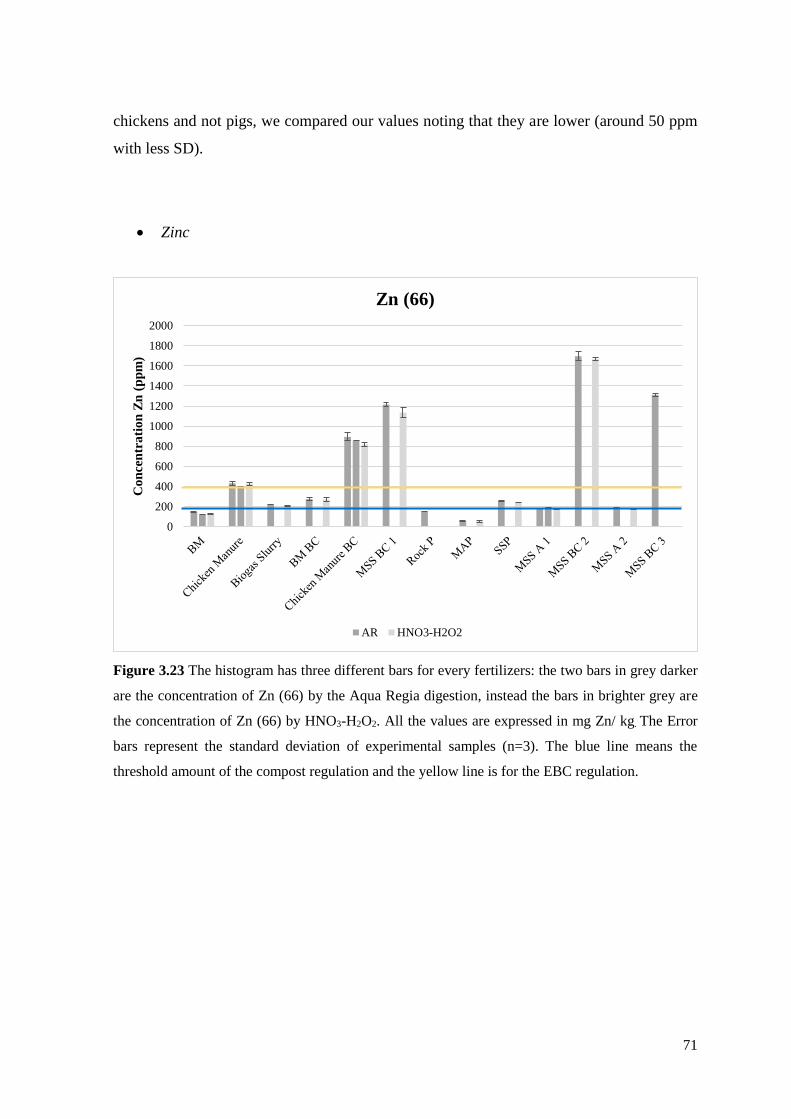
71

chickens and not pigs, we compared our values noting that they are lower (around 50 ppm

with less SD).

Zinc






0

200

400

600

800

1000

1200

1400

1600

1800

2000

Co

nce

ntr

ati

on

Zn

(p

pm

)

Zn (66)

AR HNO3-H2O2

72






In general, for Zinc the limit values are quite elevated. The lowest one (200 ppm, blue line)

are established for the compost and it is not respected by almost the entire BC and the

chicken manure. Furthermore, they are not totally in compliance with the EBC (yellow line)

that has the same value of the Swiss legislation for the general recycled fertilizers. By the

way, this one is revered by all the remain fertilizers. All the other regulations have higher

value, more than 1000 ppm, and therefore they are respected by all the samples.

A plausible explanation of the high presence of Zinc is that sometimes the feeding of the

animals is fortified with it in order to increase the proportion of multiresistant E.Coli in gut

microbial (Yazdankhah et al., 2014) or, as we said before for the Zinc case, to simply

improve the well-being and their raise they observed 653±281 mgZn/kgDM in the pig

manure. Contrasting also in this case the values of both isotopes from both digestions,

instead we saw that they were quite similar: in fact, we acquired amounts around 400 ppm

with less SD. For that reason, we can also suppose a high concentration of Zinc in the feeding

of animals.

0

200

400

600

800

1000

1200

1400

1600

1800

2000C

on

cen

tra

tio

n Z

n (

pp

m)

Zn (68)

AR HNO3-H2O2

73

Arsenic


are the concentration of As by the Aqua Regia digestion, instead the bars in brighter grey are the

concentration of As by HNO3-H2O2. All the values are expressed in mg As/kg. The Error bars

represent the standard deviation of experimental samples (n=3). The yellow line represents the EBC

regulation.

Regarding As, we compared our results only with the EBC and the Austrian Fertilizer

Regulation; for the former the threshold is 40 ppm, for the latter it is 40 mgAs/KgP2O5. As

we can see by the graph, all the concentrations detected in all the residues exceed in a great

way the limit. It is worth also with the concentration expressed in mgAs/kgP2O5 (not shown

below) because they are greater than the previous with a factor of 2.29.

Those such high values seem to represent a problem in the measurement because, comparing

our results with the previous literature, we find something strange. In the paper of Garcia

and Rosentrater (2008) the BM does not have elevated concentration of As.

0

20

40

60

80

100

120

140

160

Co

nce

ntr

ati

on

As

(pp

m)

As

AR HNO3-H2O2

74

Cadmium





regulation for the compost, instead the yellow line the EBC regulation.

0123456789

101112131415161718

Co

nce

ntr

ati

on

Cd

(p

pm

)

Cd (111)

AR HNO3-H2O2

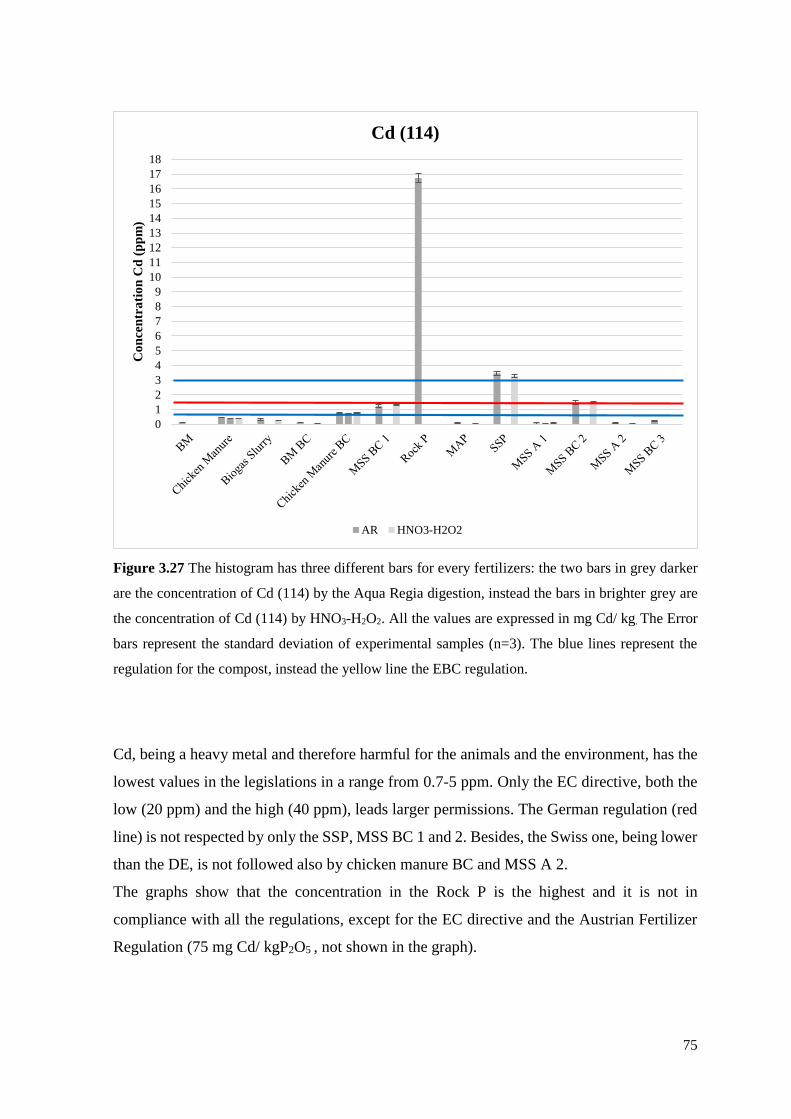
75





regulation for the compost, instead the yellow line the EBC regulation.

Cd, being a heavy metal and therefore harmful for the animals and the environment, has the

lowest values in the legislations in a range from 0.7-5 ppm. Only the EC directive, both the

low (20 ppm) and the high (40 ppm), leads larger permissions. The German regulation (red

line) is not respected by only the SSP, MSS BC 1 and 2. Besides, the Swiss one, being lower

than the DE, is not followed also by chicken manure BC and MSS A 2.

The graphs show that the concentration in the Rock P is the highest and it is not in

compliance with all the regulations, except for the EC directive and the Austrian Fertilizer

Regulation (75 mg Cd/ kgP2O5 , not shown in the graph).

0

1

2

3

4

5

6

7

8

9

10

11

12

13

14

15

16

17

18

Co

nce

ntr

ati

on

Cd

(p

pm

)Cd (114)

AR HNO3-H2O2

76

Lead


are the concentration of Pb by the Aqua Regia digestion, instead the bars in brighter grey are the

concentration of Pb by HNO3-H2O2. All the values are expressed in mg Pb/ kg. The Error bars

represent the standard deviation of experimental samples (n=3). The blue line represents the

regulation for the compost.

It is good to underline that Pb concentration revealed in the fertilizers are in compliance with

most of the legislations, because they are around or higher than 100 ppm while our results

are below 50 ppm. The only exception is with the compost ordinance of class A+ (45 ppm,

blue line) and the Austrian Fertilizer Regulation (100 mg Pb/kgP2O5, not marked in the

graph): in fact, in the MSS BC 1/ 2 that values are exceeded.

0

25

50

75

100

125

Co

nce

ntr

ati

on

Pb

(p

pm

)

Pb

AR HNO3-H2O2

77

4. DISCUSSIONS

4.1. Comparison between the two extraction methods

As it was said before a number of methods to extract P from the diverse P pools of the soil

(P dissolved in soil water; P adsorbed to surfaces of clay minerals or Fe and Al oxides, P in

primary phosphate minerals and P in organic substances and living organisms) are available

and used routinely in different countries (Wuenscher et al., 2015). Working on my thesis in

Wien, I wanted to make a comparison between DGT and the routine methods CAL (used in

Austria) as well as the Olsen method. My intention was to see if it is still worth to rely on

the current one or to move to another more reliable; the assessment was made by observing

several features: the time consuming for the preparation of the experiment and its

implementation was taken into account additionally to the correlation of the results with

plant P uptake.

Regarding the procedure of each method, they present the same one: preparation of the

solutions needed for the extraction, mixing them with the soil paste, use of the extraction

machinery and the photometric P determination. The only difference between them is the

extraction time: Olsen needs only 30 minutes in comparison to the two hours of the CAL.

Thus, from a practical point of view, the Olsen is more convenient because in a couple of

hours, it is possible to do the experiment and to obtain the results (clearly the time depends

on the number of samples).

Evaluating the phosphorus extractability, the lowest extractable amounts of P from soil were

found for the Olsen extraction method in comparison with CAL. This result is in accordance

with findings by other authors (Wuenscher et al. 2015, Fernandes et al. 1999, Csathó et al.

2005, Kulhánek et al. 2009). This assessment is visible from the box plots reported below.

78

Figure 4.1 Box plot of CAL and Olsen data series: the bottom and the top of the box are the first and

the third quartiles, and the band inside is the second quartile. The end of the whiskers is the inferior

and superior limit (corresponding to the minimum and maximum values of each data series).

CAL Olsen

First quartile (Q1 = Ƹ0.25) 21.24 10.64

Second quartile (Q2 = Ƹ0.5) 39.65 13.81

Third quartile (Q3 = Ƹ0.75) 56.01 30.91

IQR (= Q3 – Q1) 34.77 20.27

Q1 – 1.5*IQR -30.91 -19.77

Q3 + 1.5*IQR 108.16 61.31

Minimum value 12.8 9.4

Maximum value 131.0 83.9

Inferior limit Li (= max (Q1 – 1.5*IQR; minimum value)) 12.8 9.4

Superior limit Ls (= min (Q3 + 1.5*IQR; maximum value)) 131.0 83.9

Table 4.1 The value of the statistical parameters used in the box plot diagram

As can be seen from the graph above, the 50% of the Olsen’s data are lower and concentrated

in the range of 10-30 mgP/kg instead of 20-56 mgP/kg.

0

10

20

30

40

50

60

70

80

90

100

110

120

130

140

Box Plot ´CAL´

0

10

20

30

40

50

60

70

80

90

100

110

120

130

140

Box Plot ´Olsen´

79

Due to the fact that we examined only one type of soil we cannot make some considerations

about the P extractability in relation to soil properties. However, the study conducted by

Wuenscher in 2015 gave results both in accordance and in discordance with previous

researches: this underlines an uncertainty of the general knowledge about the correlation

between the P extracted and the soil properties.

In our study, different fertilizers were tested on one type of soil and as it was argued by

Kumar et al. (1994), that not only the soil but also the composition of fertilizers may

influence P extractability by different extraction methods. We also can suppose this because

only four type of recycled fertilizers gave the highest value of P in both Olsen and CAL.

They were biogas slurry, chicken manure BC, SSP and MAP. Therefore, it is possible to

think that not only the methods influence the P extractability but also the feature of the

amendments.

Further research is needed to examine the relation of P extractability by these methods to

plant P uptake in contrasting soil types and fertilizer samples.

On the other hand, correlating the amount of P with the plant P uptake shows a better linear

fitting for Olsen. It is meant that even if the quantities extracted are less they correlate in any

case better with the quantities assimilated by the plants and thus they appear more reliable.

4.2. DGT method

In the study of Mason (2008) it was provided that the diffusive thin gel method offers

benefits when predicting plant uptake/response: the use of a ferrihydrite gel as the sink

eliminates potential anionic interferences to the measurement of P that could occur by

handing an Anion Exchange Membrane and it measures P availability at more realistic soil

moisture conditions and diffusional limitation to P acquisition by plant roots. This last

feature was also previously confirmed by Zhang (2001), where observed that the presence

of a diffusive layer was the key element to mimic the plant root control on the flux, by

calculating it as the ratio between the mass of P taken and the multiplication of the exposed

gel surface and the deployment time. Later on, in a study of wheat response to an application

of P, Mason et al. (2010) underlined that the amount of phosphorous accumulated onto the

80

binding layer depends on the concentration of P in the soil pore water as well as the rate at

which P is supplied from the soil solid phase into the pore water (i.e. rate of re-supply). In

addition, they affirmed that it represents a robust technique that better assesses plant

available P and predicts the plant response to application of P, providing an improvement in

the prediction of fertilizer efficiency. Its strength lies in the fact that its reliability does not

depend on the soil type because Mason obtained these results in situations where several

factors varied, including climatic seasons, times of sowing and the use of different wheat

varieties. This key feature was also confirmed by Six et al. in the 2012.

It is known that bioassays evaluation are the most reliable methods to predict P availability.

For this reason, by analyzing the correlation of our P values obtained by the methods and

the plant responsiveness, it was understandable that the DGT showed the best fitting with

the P uptake data. For the longer time of incubation (20 days) it reported the highest value

of R2 and a better distribution of the residual errors around the zero (figure 3.7/11/15). This

strong linear correlation means that the method is able to measure P is a similar way to the

plant uptake. Thus, this comparison leads us to assess DGT as the most reliable soil-test for

plant available soil P from the tests conducted. In order to evaluate it as the best approach

such an experiment should be done with also different soils: this is a required to demonstrate

that results by DGT do not depend on the properties of soil but that it is a reliable process

for different situations.

Nevertheless, as it was shown by Mason (2010), this novel soil test has many advantages but

also some hurdles to its implementation and commercial adoption. It is time consuming

because it takes time for the preparation and for the development of the P diffusion process

to the sink. This time requirement is due to several steps: gel production, device assembly,

time of deployment, extraction and time before analysis. The two most critical steps are the

second and the third because they do not need only time for the chemical reactions or for the

waiting, but they need more time due to the precision required. The setup needs to be done

with high accuracy and rigor: the two disks gels and the two membrane do not have large

dimension and they are fragile, and their placement on the plastic support needs attention

and precision. Furthermore, the closing has to be done slowly to not create air bubbles

between the layers. Another crucial step is the deployment of the DGT because you have to

wait exactly 24 hours after the soil application (recording the exact time) before opening.

81

On the other hand, the two extraction methods did not require such a lot time for the

preparation and their development. They both needed a little lapse of time to weight the

amount of air dry soil, to make the solutions and to mix all of them in the shaking bottle.

The time depends on the number of samples but it is around a couple of hours. About the

extraction time, they demand a very brief time, 30 minutes for Olsen and 2 hours for CAL,

in juxtaposition with the 24 hours of DGT. Obviously, they also demand a high care and

rigor in the measurement, but the actions involved required less attention to the devices. In

both processes it is not required to assemble devices or to make some gels; they require only

precision regarding the weighting and the addition of extraction solution, with less effort in

comparison with the DGT.

4.3. Evaluation of the efficiency of the 13 recycled fertilizers

This study compared P fertilizer effect of a wide range of different residues rich in P,

including several varieties of each type of residue expected to differ in P availability.

Affirming that DGT was the most reliable tests, we can observe which recycling fertilizer

was more efficient to increase crop-yields.

The bar graph (figure 3.3) shows that the highest amount of P (50-180 µgP/l) was released

in the soil by recycling products as the organic fertilizers biogas slurry and chicken manure,

the thermal conversion of the chicken manure (chicken manure BC) and the struvite (MAP).

Only the standard SSP mineral fertilizer reached a value similar to the previous, due the fact

that the amount are similar, it means that the recycling fertilizers are suitable to use to

improve crops yields.

In contrast with results found in other studies (Materechera & Morutse, 2009; Petersen et

al., 2013; Delin, 2016) the P in chicken manure has an equal fertilizer value to that in mineral

fertilizer, not only in the long term but also in the short term.

The capacity of the organic waste thermochemical conversion (biochar) was also shown by

the study of Wang (2012) and Weber (2014), conducting a bioassay and chemical analysis:

by their adding to the soil, they showed an increase of shoot dry-matter yield, P concentration

and P uptake of rye grass acceptable compared with P-containing residues and fertilizers. In

our research, only the chicken manure biochar exceeded the P availability of the commercial

82

water soluble fertilizer (SSP). The MBM-BC, MSS-BC 1/2/3 reached quantities similar to

RP. These materials thus contain mainly unavailable P forms. The P in MBM is in the form

of Hydroxyapatite which would be soluble at lower soil pH values, and in the MSS-BCs P

is bound in different Fe-P species which are also insoluble.

Ashes have been shown to have variable P fertilizer effects depending on their origin. In my

thesis, the two ash samples did not perform well; Delin (2016) supposed that the justification

was the liming effect due to the high content of CaCO3 which was not favorable for P

availability in the experimental soil. Additionally, the MSS ashes used in this thesis were

experimental MSS samples which were thermo-chemically treated in an attempt to increase

P availability. Phosphorus availability in these ashes is therefore likely to be low due to the

nature of P species in MSS.

Kumar (2015) reported some data which showed that biogas slurry could easily be brought

to places that need organic fertilizers because contain considerable amount of micro and

macronutrients. As in our case, also the study of Ahmad (2009) brought in evidence an

improvement of the crop growth by the application of this ‘new’ product.

It is important to take into account that in practice, a low effect of P in residues can be

explained partly by the difficulty in applying these material with optimal placement and

timing to give the right time and way for the release of P in the soil.

To be able to strictly affirm that those products are the most efficient they should be also

compared in several soil types with diverse texture, pH, clay and Fe/Ca oxides percentage

because these variables influence P dissolution and availability to plant.

4.4. Possible contamination released by the fertilizers

Whenever a recycled material should be placed on the market as a product, it must be

registered under REACH (Registration, Evaluation, Authorization and Restriction of

Chemicals) that is the Regulation (EC) 1907/2006 is one of the EU’s endeavor to make the

use of chemicals safer. If a product is in compliance with the Fertilizer Regulation (EC)

2003/2003 it can be produced and sold anywhere in Europe; it is difficult to find a straight

phosphate fertilizer (i.e. “P-only” fertilizer) in compliance with the current regulations.

83

Based on the measurements of my research, we tried to observe if our recycled products

were in compliance with several European legislations. We conducted a general and rough

assessment in order to have a first idea about the possible contamination by ‘new’ products

obtained from wastes.

First of all, we analyzed samples from two different digestions (Aqua Regia and HNO3-

H2O2): they resulted in similar values of trace elements, with the exception of Vanadium,

Chromium, Iron, Arsenic and Lead that have less concentration with the second process. The

worst case is represented by the Vanadium, because the digested amounts differ by one order.

A possible explanation is that this kind of digestion is not able to dissolve those trace

elements species. Aqua regia is known for its complexing capacity and is better suited for

samples with a predominantly mineral matrix. Thus we can affirm that AR is a better

digestion method for those kind of products.

From the inspection of the bar-plot graphs we could understand which kind of residues

represent a possible source of soil contamination. The least efficient fertilizers were the three

biochars and the two ashes from the municipal sewage sludge (MSS BC 1/2/3 and MSS A

1/2). The content of all the trace elements studied exceeded regulations such as the

German/Swiss legislation for the recycled fertilizers or the ordinance. The chicken manure

biochar is another amendment that has high content of Copper, Cadmium and Zinc.

Concerning the mineral fertilizer, Rock P has good and safety composition, except for the

fact that it incorporates quite a large amount of Chromium and the highest level of Cadmium,

expressed in mgCd/kg. It is to be taken into account that the value of Arsenic in all fertilizers

was unusually high compared to values already reported in literature, as the one of bone meal

(Garcia et al., 2008) and of the SSA (Krüger et al., 2014). Thus, we supposed an error with

its measurement by the ICP-MS or by the preparation of the sample (digestion, dilution, …).

Furthermore, we showed that the worst feedstock was the municipal sewage sludge. In order

to verify this statement, we could compare our values with the ones obtained by Krüger et

al. (2014); they conducted a survey of all SSA in Germany and determined the respective

mass fraction of 57 trace elements over a period of one year (reported in the Appendix III).

We contrasted all our concentrations from MSS-BCs and MSS-As. In most of the cases we

achieve lower values, concerning Cadmium, Lead, Copper, Vanadium and Zinc, but the

values of Nickel and Chromium in the two ashes samples exceed them. Regarding the

84

Arsenic, we did not compare its value because it is supposed that there is something wrong

with our measurement.

The extremely low thresholds of the compost regulations are due to the fact that compost do

not have such high nutrient value and for this reason they are added at much greater level

than the fertilizers. Therefore, the compost legislations are not very relevant in the context

of contamination thresholds for fertilizers.

85

5. CONCLUSIONS

As the forthcoming depletion of global P resources is a challenge to crop production on the

long term, a change in P management and an increase of P recycling is necessary. Closing

the P cycle by using ‘residues’ as fertilizers seems to be the only solution to this challenge.

Over the years, several chemical extractions were found to be reliable for characterizing

plant P availability, but it is needed to test their accuracy for contrasting recycling fertilizers.

This research focused on the assessment of two routines (CAL and Olsen) and one new

method (DGT) to predict P availability from a representative selection of P-containing

fertilizers. These were chosen to represent the wide range of residual P-streams (e.g., animal

manure, slaughterhouse waste, products derived from municipal sewage sludge, etc.).

Moreover, to decide what residue could fit well for crop production, we examined their P

fertilizer value. This is important before application for agricultural purposes: P

bioavailability must be as high as possible to meet P crop requirement without any

wastefulness. Furthermore, a possible pollutant risk was investigated.

The data indicate that the P extracted by the extraction processes CAL and Olsen were less

in accordance than DGT with the P uptake measured with the bioassay experiment. The best

fitting with plant P uptake was reached by the DGT with longer incubation time (20 days).

Several previous studies obtained similar results: Delin (2016) found a weak prediction of P

from recycling fertilizers by the P-AL (Ammonium lactate) method, and Mason et al. (2010)

demonstrated that DGT performed better than Colwell (an NaHCO3 extraction similar to

Olsen) in a broad range of soils of different textures and pH. For these reasons, it is

concluded that DGT is a suitable method for the measurement of P availability from diverse

recycling fertilizers.

The chicken manure and its biochar, the biogas slurry and the struvite (MAP) exhibited P

availability similar to commercial mineral P (SSP). As in the studies conducted by Yusiharni

et al. (2007) and Kuligowsky et al. (2010), we obtained low P effect by the ashes; this is

likely caused by complexation of P with iron oxides, or other insoluble P species.

Trace element analysis did not show high risk of soil contamination when applied as

fertilizers. Following several European regulations, in particular the German and Swiss

regulations for recycled fertilizers, the samples that exceeded the limit values for heavy

86

metals were the residues from ashes and biochars from municipal sewage sludge, and to a

lesser extent chicken manure for (Vanadium, Zinc and Copper). It is known that animal

manures can be high in Cu and Zn due to addition in feed (Kickinger et al. 2009). Similarly,

the high Chromium, Nickel, Zinc and Copper of MSS products is in accordance with the

literature (Krüger et al. 2014).

In future, the experiment should be performed with different soils to confirm whether DGT

can predict P availability of recycling fertilizers more consistently than Olsen or CAL.

Furthermore, it would be interesting to perform it with different crops. These two matrices

are important because they entail properties (e.g., pH and buffer capacity for the soil, crop

root length/architecture and P mobilization in the rhizosphere) that can easily affect P

availability in the soil and P uptake from the plant.

87

APPENDIX I

Evaluation of plants’ condition during the pot trial

Germination Middle Harvest

# pot Type of

fertilizer

Number

of seeds

Condition

of bloom

Number

of seeds

Condition

of leaves

Number

of seeds

Condition

of leaves

1 Blank 25 good 25 dry 25 dry, h.b.

2 " 23 good 25 dry 25 dry, h.b.

3 " 22 good 24 dry 24 dry, h.b.

4 " 25 poor 25 dry 25 dry, l.b.

5 Bonemeal 25 good 25 green 25 green,

h.b.

6 " 25 good 25 dry 25 dry, h.b.

7 " 25 good 25 dry, floppy 25 dry, h.b.

8 " 25 good 25 floppy 25 green,

h.b.

9 Chicken meal 25 good 25 green 25 green,

h.b.


h.b.

11 " 25 good 25 green 25 green,

h.b.


h.b.

13 Biogas sl 25 good 25 green 25 green,

h.b.

14 Bonemeal BC 25 good 25 dry 25 dry, h.b.

15 " 25 good 25 green 25 dry, h.b.

16 " 25 ~good 25 dry 25 dry, l.b.

17 " 25 good 25 dry, floppy 25 dry, l.b.

18 Chicken M BC 25 good 25 floppy 25 green,

h.b.


h.b.

Table A.1 Report of the conditions of ryegrass during the pot trial (h.b. = high biomass, l.b.=

low biomass). The evaluation was done in three period of time: during the germination, in the

middle of the growth and at the end (harvest time).

88


# pot Type of

fertilizer

Number

of seeds

Condition

of bloom

Number

of seeds

Condition

of leaves

Number

of seeds

Condition

of leaves

20 MSS BC 25 good 25 green 25 dry, h.b.

21 " 25 good 25 dry 25 dry, h.b.

22 " 22 ~good 25 dry 25 dry, l.b.

23 " 25 good 25 dry 25 dry, l.b.

24 MSS BC 2 25 good 25 green 25 green,

h.b.

25 " 25 good 25 dry 25 dry, h.b.


h.b.

27 " 25 ~good 25 green 25 dry, h.b.

28 MSS A 1 20 poor 25 green 25 green,

h.b.


30 " 17 poor 20 green 20 dry, h.b.


h.b.

32 MSS A 2 18 poor 24 green 24 green,

h.b.

33 " 25 ~good 25 dry 25 dry, h.b.

34 " 23 poor 25 green 25 dry, h.b.


h.b.

36 Rock P 25 good 25 dry 25 dry, h.b.

37 " 25 good 25 dry 25 dry, h.b.

38 " 25 good 25 dry 25 dry, h.b.


40 SSP DC Timac 16 poor 25 floppy 25 green,

h.b.


h.b.

42 " 25 ~good 25 floppy 25 green,

h.b.


h.b.

Table A.1 Report of the conditions of ryegrass during the pot trial (h.b. = high biomass, l.b.=

low biomass). The evaluation was done in three period of time: during the germination, in the

middle of the growth and at the end (harvest time).

89


# pot Type of

fertilizer

Number

of seeds

Condition

of bloom

Number

of seeds

Condition

of leaves

Number

of seeds

Condition

of leaves

44 MAP 25 good 25 floppy 25 green,

h.b.


h.b.


h.b.


h.b.

48 MSS BC 3 25 good 25 dry 25 dry, l.b.

49 " 25 good 25 dry 25 dry, l.b.

50 " 25 good 25 dry 25 dry, l.b.

51 " 25 good 25 dry 25 dry, l.b.

Table A.1 Report of the conditions of ryegrass during the pot trial (h.b. = high biomass, l.b.= low

biomass). The evaluation was done in three period of time: during the germination, in the middle of

the growth and at the end (harvest time).

During this research I reported all the characteristics of the plants’ growth (6 weeks): in the

table above the appearance in the first week (the germination phase), in the third (in the

middle of the growth) and in the last week (the harvest phase) is described.

As we can see not all the seeds germinated at the same time: the majority of the pots achieved

the number already in the first week but some took two weeks to have 25 seeds germinated.

At the sixth week, we found 25 plants in each pot with the exception of one pot of control

and two pots fertilized with MSS A 1 and MSS A 2. Despite of this fact, most seeds

germinated in a good way (fig. 5.1).

90

Figure A.1 Ryegrass seeds in germination.

After three weeks, when the leaves reached a size of ca. 25 cm, we started to monitor the

color and the strength of the leaflets in order to check their health. A green color is a symbol

of a good well-being, instead a yellow color indicates a deficiency (e.g. iron, N, Mg), If the

iron is present in small quantities the vegetative development is arrested and the chlorophyll

doesn’t form anymore (‘chlorosis’ is the condition in which the chlorophyll is not produced

in sufficient quantities); this happens because it is an element, together with the magnesium,

fundamental in the composition of the chlorophyll molecule. In our research we had different

situations: some of them showed yellow and dry leaves but vital (e.g. the pot corresponding

to the fertilizers MSS BC 3, Rock P, Bonemeal and MSS BC), other exhibited green but

floppy leaves (MAP and SSP) and the remainder was in a healthy condition status. Due to

the presence of ‘chlorosis’ in some scattered pots, we sprayed Iron Sulphate 3% two times.

At the time of the harvest the pots fertilized with MSS BC 3, Rock P, Bonemeal and MSS

BC did not demonstrate any changes in the aspect they presented again some dry leaves.

Regarding the quantity of biomass grown, it was high in the majority of the pots except for

the ones fertilized with the MSS BC 3 (in all the four replicates) and for two replicates out

of four in the cases of Bonemeal BC and MSS BC.

Figures are shown below, that display the difference between the situation of small and large

biomass.

91

Example of low biomass Examples of high biomass

Figure A.2 Pot with MSS BC 3 Figure A.3 Pot with SSP

Figure A.4 Pot with MSS BC Figure A.5 Pot with Chicken manure

92

APPENDIX II

Analysis of phosphate using molybdate blue colorimetry (in-house method by Jakob

Santner, 2013)

The test referred to Murphy J. and Riley J. P. (1962), a modified single solution method for

the determination of phosphate in natural waters (Anal. Chim. Acta 27, 31-36). The principle

of this procedure is that the phosphate and the molybdate ions form a complex that turns

blue upon reduction by ascorbic acid. Its quantification limit is 0.010 mg P l-1.

The solutions needed for the preparation of the staining reagents are:

- H2SO4 2.5 mol l-1 (A): topping up 25.5 g at 96% H2SO4 to 100 ml deionized water in

a becker;

- B: dissolving 10 g ammonium heptdamolybdate tetrahydrate in water and reaching

the level of 250 ml;

- C: dissolving 0.28g potassium antimonyltartrate hydrate in deionized water reaching

the level of 100 ml;

- D: dissolving 0.88g of ascorbic acid in deionized water topping up to 50 ml.

The staining reagents can be of two types:

- SR1 for samples not containing H2SO4 : obtained by mixing together 10 ml of A, 3

ml of B, 1 ml of C and 6 ml of D;

- SR2 for samples containing 0.25 M H2SO4 : mixing 10 ml of deionized water with 3

ml of B and 1 ml of C.

A, B and C can be stored at room temperature for several months. Instead, D and the staining

reagents have to be prepared daily.

The method is linear in the range 10-500 (sometimes 750/1000) µg P l-1. It is necessary to

be sure to calculate the standards correctly for each method.

93

For preparing the samples:

- adding 0.2 ml SR1 to 1 ml of sample, without acid inside, and let’s react for 15-20

minutes;

- adding 0.14 ml SR2 and 0.06 ml D to 1 ml of sample 0.25 M H2SO4 and let’s react

for 15-20 minutes.

Afterwards the analysis is done by UV/VIS spectrophotometer at a wavelength of 881 nm.

In this research the preparation of the standards and the samples was different for each

chemical analysis studied:

- Olsen method:

For the preparation of the standards and the samples we pipetted 25 ml of NaHCO3

extract into 50 ml volumetric flask, adding one or two drops of phenolphthalein.

2.625 ml of H2SO4 2.5 M were needed to turn the phenotphtalein colorless meaning

that all carbonates were removed. The desired concentration range of standards was:

0, 0.065, 0.196, 0.326, 0.457, 0.587 and 0.717 µg P l-1 in NaHCO3 matrix and it was

reached by adding 0, 1, 3, 5, 7, 9 and 11 ml of the base P standard (it was stored in a

volumetric flask of 50 ml of 3.26 mg P/l) to 50 ml volumetric flask., then bringing

them to the volume with HQ water. For the samples, depending on the fertilizer P

content and solubility we did one or two dilution:

- Dilution step 1 (1:2.05) with 5 ml Olsen extract + 5.25 ml H2SO4 0.25M and

- Dilution step 2 for the samples containing more P: (1:2) with 0.5 ml of step 1 + 0.5

ml of 0.125M Na2SO4 or (1:3) 0.33 ml sample from step 1 + and 0.66 ml of 0.125M

Na2SO4 .

- Calcium Acetate - Calcium Lactate (CAL) method:

The calibration standards were prepared from the phosphate stock solution according

to the table below.

94

A 0.1 ml calibration standard or sample, followed by 1.6 ml dilute dye solution and

0.5 ml ascorbic acid solution, are mixed and well shaken. The mixture is transferred

to a single-use colorimeter cuvette.

Nominal P

concentrati

on (mg l-1)

Total

volu

me

(ml)

P

standard

stock

(ml)

Standard

5 (ml)

Extractant

stock (ml)

Lab

water

(ml)

Cal. Blank 0 10 - - 2.00 8.00

Std 1 1 10 - 0.40 2.00 7.60

Std 2 5 10 0.15 - 2.00 7.85

Std 3 10 10 0.31 - 2.00 7.69

Std 4 15 10 0.46 - 2.00 7.54

Std 5 25 10 0.77 - 2.00 7.23

Table A.2 Volume needed for the preparation of the calibration standard solutions in the

CAL method.

- Diffusive Gradient in Thin Gel (DGT):

We prepared 45 ml for each standards following the data reported in the table below

(Table 5.3).

P conc (mg/l) P-std diluted

(10 mgP/l)

(ml)

2.5M H2SO4

(ml)

H2O (ml)

Blank 0.00 0.00 4.50 40.50

Std 1* 0.02 1.80 4.50 38.70

Std 2 0.10 0.45 4.50 40.05

Std 3 0.20 0.90 4.50 39.60

Std 4 0.30 1.35 4.50 39.15

Std 5 0.40 1.80 4.50 38.70

Std 6 0.50 2.25 4.50 38.25

*Prepare last by pipetting from Std 6

Table A.3 Volume needed for the preparation of the calibration standard solutions in the

DGT method.

95

For the calibration line we used P standards in 0.25M H2SO4 and the range chosen

was: 0.02, 0.1, 0.2, 0.3, 0.4 and 0.5 mg P l-1. Standards and elutates of the DGT

samples were stained according to the blue colorimetric method for samples

containing H2SO4 as described above.

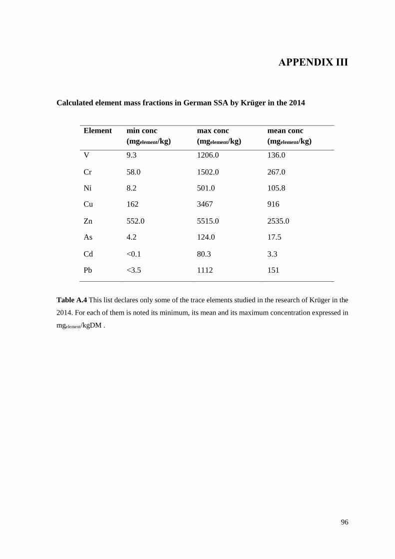
96

APPENDIX III

Calculated element mass fractions in German SSA by Krüger in the 2014

Element min conc

(mgelement/kg)

max conc

(mgelement/kg)

mean conc

(mgelement/kg)

V 9.3 1206.0 136.0

Cr 58.0 1502.0 267.0

Ni 8.2 501.0 105.8

Cu 162 3467 916

Zn 552.0 5515.0 2535.0

As 4.2 124.0 17.5

Cd <0.1 80.3 3.3

Pb <3.5 1112 151

Table A.4 This list declares only some of the trace elements studied in the research of Krüger in the

2014. For each of them is noted its minimum, its mean and its maximum concentration expressed in

mgelement/kgDM .

97

REFERENCES

Aggelides S.M., Londra P.A., (2000) Éffects of compost produced from town wastes and sewage

sludge on the physical properties of a loamy and clay soil´, Bios. Techn. (71):253-259.

Ahmad, R., Jabeen, N., (2009) ´Demonstration of growth improvement in sunflower (helianthus

annuus l.) by the use of organic fertilizers under saline conditions´ Pak. J. Bot. 41(3), 1373-1384.

Al Sayed M.H., Madany I.M., Buali A.R.M., (1995), Constr. Build. Mater. 9 (1), 19–23.

Atkinson C. J., Fitzgerald J. D., Hipps N. A. (2010) ´Potential mechanisms for achieving agricultural

benefits from biochar application to temperate soils: a review´. Plant Soil (337), 1–18.

Baur R..J., 2009, ´Waste activated sludge stripping to remove internal phosphorus´, US patent

7604740B2.

Bundesamt für Umwelt, Wald und Landschaft (BUWAL) (2004), ´Schriftenreihe Umwelt Nr. 368.

Boden, Phosphor in Böden Standortbestimmung Schweiz´. Herausgegeben vom Bundesamt für

Umwelt, Wald und Landschaft BUWAL Bern.

Cabeza R., Steingrobe B., Römer W., Claassen N., (2011) Éffectiveness of recycled P products as

P fertilizers, as evaluated in pot experiments´, Nutr. Cycl. Agroecosyst. (91): 173-184.

Chen L., Lin D.F., Hazard J., (2009), ´Stabilisation treatment of soft subgrade soil by sewage sludge

ash and cement´, Mater. 162 (1), 321–327.

Christel W., Lemming C., Mundus S., Bruun S., Jakob, Magid J., Jensen L.S., (2016), ´Measuring

phosphorus availability in recently fertilized soils with the diffusive gradient in thin films (DGT)

method – challenges and opportunities´, Comm. in Soil Scien. and Plant Anal.

Christel, W., S. Bruun, J. Magid, L. S. Jensen, (2014), ´Phosphorus availability from the solid

fraction of pig slurry is altered by composting or thermal treatment´, Biores. Techn. (169):543–51.

Claassen N., Steingrobe B., Pérez R. C. (2010) ´Phosphorrecycling – Charakterisierung der

Düngewirkung recyclierter Phosphatdünger in Feld- und Gefäßversuchen´, Abschlus. BMBF,

Förderkennzeichen 02WA0786.

Cooper J., Lombardi R., Boardman D., Carliell-Marquet C., (2011) ´The future distribution and

production of phosphate rock reserves´, Resour., Conser. and Recycl. (57): 78-86.

Compost Ordinance (FLG II Nr. 292/2001).

Cordell D., Drangert J.O., White S., (2009) ´The story of phosphorus: global food security and food

for thought´, Global Environ. Change (19):292-305.

Csathó P., Magyar M., Debreczeni K., Sárdi K., (2005), Ćorrelation between soil P and wheat shoot

P contents in a network of Hungarian long-term field trials´ Communi. in Soil Science and Plant

Anal., (36): 275–293.

De Ridder M., S. De Jong, J. Polchar, Lingemann S., (2012), ´Risks and opportunities in the global

phosphate rock market: Robust strategies in times of uncertainty´, (HCSS) Report.

Degryse F., Smolders E., Zhang H., Davison W., (2009), ´Predicting availability of mineral elements

to plants with the DGT technique: a review of experimental data and interpretation by modelling´,

Environ. Chem. (6):198-218.

Delin S., (2016), ´Fertilizer value of phosphorus in different residues´, Soil Use and Manag., (32),

17-26.

Deutsche Bundes-Bodenschutz- und Altlastenverordnung (BBodSchV), (1999), latest amendment

31.7.2009.

Düngemittelverordnung (DüMV – DE Regulation) currently under recast 19.12.2008

Düngerbuch-Verordnung (DüBV – Swiss Regulation) enforced 16.11.2007.

Dikov G., Hermann L., Hukari S., Muskolus A., Nättorp A., Pokorna M., de Ubieta C.G., (2012)

´Pre-Normative matrix. Review of fertilization schemes. Review of current legal framework for

98

phosphorus recovery´, Project supported by the European Commission within the Seventh Frame-

work Programme Grant agreement No. 308645 (P-REX).

Fernandes M.L.V., Indiati R., Countinho J., Buondonno A., (1999), ´Soil properties affecting

phosphorus extraction from Portuguese soils by conventional and innovative methods´ Comm. in

Soils Science and Plant Anal., (30): 921–936.

Garcia R.A., Rosentrater K.A., (2008) Ćoncentration of key elements in north American meat and

bone meal´, Biom. and Bioen. (32):887-891.

Gesamte Rechtsvorschrift für Düngemittelverordnung (Austrian Fertilizer Regulation) 2004,

enforced 27.11.2016.

Agricultural Committee of ISMA, (1980), Handbook on Phosphate Fertilization.

Hinsinger P., Plassard C., Tang C.X., Jaillard B., (2003) Órigins of root-mediated pH changes in the

rhi-zosphere and their responses to environmental constraints: A review´ Plant Soil (248):43 – 59.

ICP MS Interferenz Tabelle, Finnigan MAT, Bremen, 1995.

Jaffer Y., Clark T., Pearce P., Parsons S., (2002), ´Potential phosphorus recovery by struvite

formation´, Water Res. (36):1834–1842.

Jasinski B. S. M., (2005), ´Mine-rals Yearbook´, U.S. Geological Survey, 2013.

Johnston E.A., Poulton P. R., Fixen P. E., Curtin D., (2014) ´Phosphot´rus: its efficient use in

agriculture´, Advan. in Agron., (123): 177-228.

Kammann, C., Linsel, S., Gößling, J. W., Koyro, H. (2011) Ínfluence of biochar on drought

tolerance of Chenopodium quinoa Willd and on soil–plant relations´ Plant Soil (345): 195–210.

Kamprath E.J., Watson M.E., (1980) Ćonventional soil and tissue tests for assessing the phosphorus

status of soil`, The role of Phosphorus in Agriculture:.433-469.

Kauthale V.K., Takawale P.S., Kulkarn, P.K., Daniel L.N., (2005) Ínfluence of fly ash and sewage

sludge application on growth and yield of annual crops´, Intern. Journ. of Tropical Agricul. (23):49-

54.

Kickinger T., Würzner H., Windisch W., (2009), ´Zinc and Copper in feeds, slurry and soils from

Austrian pig fattening farms feeding commercial complete feed or feed mixtures produced on-farm´,

Die Bodenkultur, 60 (4).

Kreuzeder, A., Santner J., Zhang H., Prohaska T., Wenzel W., (2015), Úncertainty evaluation of the

diffusive gradients in thin films technique´, Environ. Science & Techn. 49 (3):1594–602.

Krüger O., Grabner A., Adam C., (2014), ́ Complete survey of german sewage sludge ash’, Environ.l

Science and Techn.

Kulhánek M., Balík J., Černý J., Vaněk V., (2009), Évaluation of phosphorus mobility in soil using

different extraction methods´, Plant, Soil and Environ.t, (55): 267–272.

Kuligowski K., Poulsen T., Rubæk, G., Sørensen, P. (2010), ´Plant availability to barley of

phosphorous in ash from thermally treated animal manure in comparison to other manure based

materials and commercial fertilizer´, European Journal of Agronomy, (33):293-303.

Kumar S., Malav L.C., Malav Kumar M., Khan A.S., (2015) ´Biogas Slurry: Source of Nutrients for

Eco-friendly Agriculture´, International J. Ext. Res. (2):42-46.

Kumar V., Bolland M.D.A., Gilkers R.J. (1994), Ćomparison of the Pi, Colwell, Bray 1, calcium

lactate (CAL) and Truog soil phosphorus test for predicting growth of oats, barley, triticale and clover

in the field in lateritic soils fertilized with superphosphate and rock phosphate´, Fertil. Resear., (37):

115-124.

Kumar V., Chopra A.K., 2013, Áccumulation and translocation of metals in soil and different parts

of French Bean (Phaseolus vulgaris L.) amended with sewage sludge´, Bull. Environ. Contam.

Toxicol.

Liebig J., (1840), ´Die organische Chemie in ihrer Anwendung auf Agri- und Physiologie (Organic

chemistry in its applications to agriculture and physiology)´, Friedrich Vieweg und Sohn Publ, Co.

Lin, D.F., Lin, K.L., Hung, M.J., Luo, H.L., J. Hazard., (2007), ´Sludge ash/hydrated lime on

geotechnical properties of soft soil´, Mater. 145 (1–2): 58–64.

Liu T., Liu B., Zhang W., (2014) Ńutrient and Heavy metal in biochar produced by sewage sludge

pyrolysis: its application in soil amendment´, Pol. J. Environ. Stud. 23(1): 271-275.

99

Mason S., Hamon R., Zhang H., Anderson J., (2008), Ínvestigating chemical constraints to the

measurement of phosphorus in soils using diffusive gradients in thin films (DGT) and resin methods´,

Talanta (74): 779-787.

Mason S., McNeill A., McLaughlin M., Zhang H., (2010), ´Prediction of wheat response to an

application of phosphorus under field conditions using diffusive gradients in thinfilms (DGT) and

extraction methods´, Plant Soil (337):243-258.

Mason S.D., McLaughlin M.J., Johnston C., McNeill A., (2013), ´Soil test measures of available P

(Colwell, resin and DGT) compared with plant P uptake using isotope dilution´, Plant Soil.

Materechera S.A., Morutse H.M., (2009) ´response of maize to phosphorus from fertilizer and

chicken manure in a semi-arid environment of south africa´, Experim. Agricult., 45 (3):261-273.

Mengel K., Kirkby E.A. (2001), `Principles of plant nutrition´ Dordrecht: Kluwer Academic

Publishers.

Moody P.W., Speirs S.D., Scott B.J., Mason S.D., (2013), ´Soil phosphorus tests I: What soil

phohphorus pools and processes do they measure?´, Crop & Pasture Science, (64):461-468.

Mtshali J.S., Tiruneh A.T., Fadiran A.O., (2014), Ćharacterization of sewage sludge generated from

wastewater treatment plants in Swaziland in relation to agriculture uses´, Resour. and Environ., 4(4):

190-199.

Myint K. (2005) ́ Short- and long-term P dynamics of various P fractions in the field and in the rhizo-

sphere´, Ph.D. Thesis, Georg-August-Universität, Göttingen.

Nye P.H.,(1980), ´Diffusion of ions and unchanged solutes in soils and clays´, Advanc. in Agron.,

(31):225-272.

Oelkers E.H., Valsami-Jones E., (2008), ´Phosphate mineral reactivity and global sustainability´,

Elements (4): 83-87.

Olsen S.R., Cole C.V., Watanabe F.S., Dean L.A., (1954), Éstimation of available phosphorus in

soils by extraction with sodium bicarbonate´, USDA Circular 939, U.S. Government Printing Office,

1–19.

Petersen, J., Lemming, C., Rubæk, G., Sørensen, P. (2013) ´Sideband injection of acidified cattle

slurry as starter P-fertilization for maize seedlings´ Proceedings from 15th RAMIRAN International

Conference, Versailles, France, 3–5 June 2013.

Pote D.H., Daniel T.C., Sharpley A.N., Moore P.A. Jr., Edwards D.R., Nichols D.J., (1996),

´Relating extractable soil phosphorus to phosphorus losses in runoff´, Soil Sci. Soc. Am. J., (84):275-

281.

Reijnders L., (2014), ´Phosphorus resources, their depletion and conservation, a review´, Resour.

Conserv. Recycl., 93:32-49.

Richardson A.E., Barea J.-M., McNeill A. M., Prigent-Combaret, C. (2009) Ácquisition of

phosphorus and nitrogen in the rhizosphere and plant growth promotion by microorganisms´ Plant.

Soil. (321):305 – 339.

Römer W. (2013a) ´Gehaltsklassen neu bewerten?´, DLG-Mitteilungen Heft 5, Jahrgang 2013

Eschborner Landstraße 122, 60489 Frankfurt/Main.

Römer W. (2013b) ´Phosphor-Düngewirkung von P-Recyclingprodukten´ Korrespondenz-

Abwasser-Abfall, KA 2013/06.

Ruth E. Wolf, (2005) ´What is ICP-MS? … and more importantly, what can it do?´ Ph.D. Research

Chemist, USGS/CR/CICT.

Sample E.C., Soper R.J., Racz G.J. (1980). ´Reactions of phosphate fertilizers in soils´, Khasawneh,

F.E., Sample E.C., Kamprath E.J. (1980) ´The Role of Phosphorus in Agriculture´, Amer. Soc. of

Agron., Crop Sci. Soc. Amer. and Soil Sci. Soc. Amer.: 263-310.

Santner J., Mannel M., Burrell L. D., (2014), ´Phosphorus uptake by Zea mays L. is quantitatively

predicted by infinite sink extraction of soil P´, Plant Soil.

Santner J., Prohaska T., Luo J., Zhang H., (2010), ´Ferrihydrite containing gel for chemical imaging

of labile phosphate species in sediments and soils using diffusive gradients in thin films´, Anal.

Chem., (82): 7668-7674.

Sanyal S.K., De Datta S.K. (1991), Ćhemistry of phosphorus transformations in soil´, Advan. in Soil

Science. (16):1-120.

https://www.cambridge.org/core/journals/experimental-agriculture/volume/journal-eag-volume-45/E81BC488F3F90B0CBA893667205204E1

100

Sattari S.Z., Bouwman A.F., Giller K.E., van Ittersum M.K., (2012), ´Residual soil phosphorus as

the missing piece in the global phosphorus crisis puzzle´, Proc. Natl. Acad. Sci., (109):6348-6353.

Schauer P., Baur R., Barnard J., Britton A., (2011), Íncreasing revenue while reducing nuisance

struvite precipitation: pilot scale testing of the WASSTRIP process´, Proc. Water Environ. Fed.

Schoenau J.J., O´Halloran I.P., (2007), ´Sodium bicarbonate-extractable phosphorus´, Soil sampling

and methods of Anal.: 89-94.

Scholz R.W., Wellmer F.W., (2013), Ápproaching a dynamic view on the availability of mineral

resources: what we may learn from the case of phosphorus?´, Glob. Environ. Chang. (23): 11-27.

Schoumans O.F., Bouraoui F., Kabbe C., Oenema O., Van Dijk K.C., (2015), ´Phosphorus

management in Europe in a changing world´, AMBIO, 44(Suppl.2): S180-S192.

Schröder J.J., Smit A.L., Cordell D., Rosemarin A., (2011), Ímproved phosphorus use efficiency in

agriculture: a key requirement for its sustainable use´, Chemo. (84):822-831.

Schrödter K., Bettermann G., Staffel T., Wahl F., Klein T., Hofmann T., (2012), ´Phosphoric Acid

and Phosphates´, Ullmann’s encyclopedia of industrial chemistry :679–724.

Sharpley A.N., Chapra S.C., Wedepohl R., Sims J.T., Daniel T.C., Reddy K.R., (1994), ´Managing

agricultural phosphorus for protection of surface waters: issues and options´, J. Environ. Qual.,

(23):437-441.

Sims J.T., (2000), ´Soil test phosphorus: Olsen P.´, Methods of Phosphorus Analysis for soils,

sediments, residuals, and water:20-21.

Six L., Pypers P., Degryse F., Smolders E., Merckx R., (2012), ´The performance of DGT versus

conventional soil phosphorus tests in tropical soils- an isotope dilution study´, Plant Soil (359):267-

279.

Turner B.L., Kay M.A., Westermann D.T., (2004), ´Phosphorus in surface runoff from calcareous

arable soils of the semiarid western United States´, J. Environ. Qual., (33): 1814-1821.

Tyler G., Jobin S.A.S, (1995) ´ ICP-OES, ICP-MS and AAS Techniques Compared´, ICP Optical

Emission Spectroscopy Technical note 05.

U.S.G. Survey, (2014), ´Phosphate rock´, Mineral commodity summaries, ed. S. Jewell and S.M.

Kimball, 196 pp. Reston, VA: U.S. Geological Survey.

Van Dijk K.C., Lesschen J.P., Oenema O., (2016), ´Phosphorus flows and balances of the European

Union Member States´, Science of the Tot. Environ., (542): 1078-1093.

Wang T., Camps-Arbestain M., Hedley M., Bishop P., (2012), ́ Predicting phosphorus bioavailability

from high-ash biochars´, Plant Soil (357): 173-187.

Weber B., Stadlbauer E. A., Schlich E., Eichenauer S., Kern J, Steffens D., (2014), ´Phosphorus

bioavailability of biochars produced by thermo-chemical conversion´, J. Plant Nutr. Soil Sci., (177):

84-90.

Withers P.J.A., Sylvester-Bradley R., Jones D.L., Healey J.R., Talboys P.J., (2014), ´ Feed the crop

not the soil: rethinking phosphorus management in the food chain´, Environ. Sci. Technol. (48):6523-

6530.

Wong J,W,C, Li S.W.Y. and Wong M.H., (1995), Ćoal fly ash as composting material for sewage

sludge: effects on microbial activities´, Environ. Technol. (16):527–537.

Wuenscher R., Unterfrauner H., Peticzka R., Zehetner F., (2015), Á comparison of 14 soil

phosphorus extraction methods applied to 50 agricultural soils from Central Europe´, Plant Soil

Environ., 61(2): 86-96.

Yazdankhah S., Rudi K., Bernhoft A., (2014), ´Zinc and Copper in animal feed – development of

resistance and co-resistace to antimicrobial agents in bacteria of animal origin´, Microbial Ecology

in Health and Disease.

Yusiharni B.E., Ziadi H., Gilker R.J., (2007), Á laboratory and glasshouse evaluation of chicken

litter ash, wood ash and iron smelting slag as liming agents and P fertilizers´, Australian J. of soil

resear., (45): 374-389.

Zhang H., Davison W., (1995), ´Performance characteristics of diffusion gradients in thin films for

the in situ measurement of trace metals in aqueous solution´, Anal. Chem. (67):3391-3400.

Zhang H., Zhao F.J., Sun B., Davison W., McGrath S.P., (2001) Envi. Sci. Technol. (35): 2602.

101

Zorn W., Krause O., (1999), ´ Untersuchungen zur Charakterisierung des pflanzenverfügbaren

Phosphats in Thüringer Carbonatböden´, J. of plant nutr. and soil science.

WEB RESOURCES

The Gasification and Syngas Technologies Council (2016), ´Gasification vs Pyrolysis´, [online]

available at: www.gasification-syngas.org/applications/gasification-vs.-pyrolysis/ [accessed

September 2016].

SunCoal Industries GmbH, (2013) ´Hydrothermal Carbonization, [online] available at:

http://www.htc-labs.org/en/hydrothermal-carbonisation/ [accessed September 2016].

RETSCH, ´Mixer Mill MM 200´ (Figure 2.1), [online] available at:

http://www.retsch.com/products/miling/ball-mills/mixer-mill-mm-200/ [accessed July 2016].

All Recycling Facts, (2014) ´Why use organic fertilizers?´, [online] available at: http://www.all-

recycling-facts.com/organic-fertilizer.html [accessed August 2016].

International Plant Nutrition Institute, ´Phosphate Rock´ (No 19), (2010) [online] available

at:https://www.ipni.net/publication/nss.nsf/0/89BE55B22373F573852579AF00767AFE/$FILE/NS

S-19%20Phosphate%20Rock.pdf [accessed August 2016].

Pavlis R. (2014), ´Rock phosphate fertilizer´, [online] available at:

http://www.gardenmyths.com/rock-phosphate-fertilizer/ [accessed August 2016].

International Plant Nutrition Institute, ´ Single Superphosphate (No 21), (2010) [online] available

at:https://www.ipni.net/publication/nss.nsf/0/5540C741907C7657852579AF007689EC/$FILE/NS

S-21%20SSP.pdf [accessed August 2016].

BOHRA INDUSTRIES LTD. ´Single Superphosphate (SSP)´, (2015) [online] available at:

http://www.bohraindustries.com/ssp.html [accessed August 2016].

EUROSTAT, ´Gross Phosphorus balance´ (2014), [online] available at:

http://ec.europa.eu/eurostat/tgm/table.do?tab=table&init=1&language=en&pcode=t2020_rn310&pl

ugin=1 [accessed July 2016].

P-REX EU Project, [online] available at: http://www.p-rex.eu/ [accessed September 2016].

Eurostat [online] available at: http://epp.eurostat.ec.europa.eu/portal/page/portal/eurostat/home/

Rhoades H. (2016) ´Using chicken manure fertilizer in your garden´ [online] available at:

www.gardeningknowhow.com [accessed August 2016].

VDLUFA (1997) ´Phosphordüngung nach Bodenuntersuchung und Pflanzenbedarf´, [online]

available at: http://www.vdlufa.de/joomla/Dokumente/Standpunkte/0-4-phosphor.pdf [accessed

August 2016].

European Directives, [online] available at: http://eur-lex.europa.eu/ [accessed October 2016].

http://www.gasification-syngas.org/applications/gasification-vs.-pyrolysis/

http://www.htc-labs.org/en/hydrothermal-carbonisation/

http://www.retsch.com/products/miling/ball-mills/mixer-mill-mm-200/

http://www.all-recycling-facts.com/organic-fertilizer.html

http://www.all-recycling-facts.com/organic-fertilizer.html

https://www.ipni.net/publication/nss.nsf/0/89BE55B22373F573852579AF00767AFE/$FILE/NSS-19%20Phosphate%20Rock.pdf

https://www.ipni.net/publication/nss.nsf/0/89BE55B22373F573852579AF00767AFE/$FILE/NSS-19%20Phosphate%20Rock.pdf

http://www.gardenmyths.com/rock-phosphate-fertilizer/

https://www.ipni.net/publication/nss.nsf/0/5540C741907C7657852579AF007689EC/$FILE/NSS-21%20SSP.pdf

https://www.ipni.net/publication/nss.nsf/0/5540C741907C7657852579AF007689EC/$FILE/NSS-21%20SSP.pdf

http://www.bohraindustries.com/ssp.html

http://ec.europa.eu/eurostat/tgm/table.do?tab=table&init=1&language=en&pcode=t2020_rn310&plugin=1

http://ec.europa.eu/eurostat/tgm/table.do?tab=table&init=1&language=en&pcode=t2020_rn310&plugin=1

http://www.p-rex.eu/

http://epp.eurostat.ec.europa.eu/portal/page/portal/eurostat/home/

http://www.gardeningknowhow.com/

http://www.vdlufa.de/joomla/Dokumente/Standpunkte/0-4-phosphor.pdf

http://eur-lex.europa.eu/

from waste to fertilizer: evaluation of waste and waste

Documents