From "Think Like a Vertex" to "Think Like a Graph"

Yuanyuan Tian†, Andrey Balmin§ 1, Severin Andreas Corsten?, Shirish Tatikonda†, John McPherson††IBM Almaden Research Center, USA {ytian, statiko, jmcphers}@us.ibm.com

§GraphSQL, USA andrey@graphsql.com?IBM Deutschland GmbH, Germany severin.corsten@de.ibm.com

ABSTRACTTo meet the challenge of processing rapidly growing graph andnetwork data created by modern applications, a number of dis-tributed graph processing systems have emerged, such as Pregel andGraphLab. All these systems divide input graphs into partitions,and employ a “think like a vertex” programming model to supportiterative graph computation. This vertex-centric model is easy toprogram and has been proved useful for many graph algorithms.However, this model hides the partitioning information from theusers, thus prevents many algorithm-specific optimizations. Thisoften results in longer execution time due to excessive networkmessages (e.g. in Pregel) or heavy scheduling overhead to ensuredata consistency (e.g. in GraphLab). To address this limitation, wepropose a new “think like a graph” programming paradigm. Underthis graph-centric model, the partition structure is opened up to theusers, and can be utilized so that communication within a partitioncan bypass the heavy message passing or scheduling machinery. Weimplemented this model in a new system, called Giraph++, based onApache Giraph, an open source implementation of Pregel. We ex-plore the applicability of the graph-centric model to three categoriesof graph algorithms, and demonstrate its flexibility and superiorperformance, especially on well-partitioned data. For example, ona web graph with 118 million vertices and 855 million edges, thegraph-centric version of connected component detection algorithmruns 63X faster and uses 204X fewer network messages than itsvertex-centric counterpart.

1. INTRODUCTIONRapidly growing social networks and other graph datasets require

a scalable processing infrastructure. MapReduce [7], despite its pop-ularity for big data computation, is awkward at supporting iterativegraph algorithms. As a result, a number of distributed/parallel graphprocessing systems have been proposed, including Pregel [15], itsopen source implementation Apache Giraph [1], GraphLab [14],Kineograph [6], Trinity [20], and Grace [23].

The common processing patterns shared among existing dis-tributed/parallel graph processing systems are: (1) they divide inputgraphs into partitions for parallelization, and (2) they employ a

This work is licensed under the Creative Commons Attribution-NonCommercial-NoDerivs 3.0 Unported License. To view a copy of this li-cense, visit http://creativecommons.org/licenses/by-nc-nd/3.0/. Obtain per-mission prior to any use beyond those covered by the license. Contactcopyright holder by emailing info@vldb.org. Articles from this volumewere invited to present their results at the 40th International Conference onVery Large Data Bases, September 1st - 5th 2014, Hangzhou, China.Proceedings of the VLDB Endowment, Vol. 7, No. 3Copyright 2013 VLDB Endowment 2150-8097/13/11.

vertex-centric programming model, where users express their al-gorithms by “thinking like a vertex”. Each vertex contains infor-mation about itself and all its outgoing edges, and the computationis expressed at the level of a single vertex. In Pregel, a commonvertex-centric computation involves receiving messages from othervertices, updating the state of itself and its edges, and sending mes-sages to other vertices. In GraphLab, the computation for a vertex isto read or/and update its own data or data of its neighbors.

This vertex-centric model is very easy to program and has beenproved to be useful for many graph algorithms. However, it does notalways perform efficiently, because it ignores the vital informationabout graph partitions. Each graph partition essentially represents aproper subgraph of the original input graph, instead of a collectionof unrelated vertices. In the vertex-centric model, a vertex is veryshort sighted: it only has information about its immediate neighbors,therefore information is propagated through graphs slowly, one hopat a time. As a result, it takes many computation steps to propagatea piece of information from a source to a destination, even if bothappear in the same graph partition.

To overcome this limitation of the vertex-centric model, we pro-pose a new graph-centric programming paradigm that opens upthe partition structure to users and allows information to flow freelyinside a partition. We implemented this graph-centric model in anew distributed graph processing system called Giraph++, which isbased on Apache Giraph.

To illustrate the flexibility and the associated performance advan-tages of the graph-centric model, we demonstrate its use in threecategories of graph algorithms: graph traversal, random walk, andgraph aggregation. Together, they represent a large subset of graphalgorithms. These example algorithms show that the graph-centricparadigm facilitates the use of existing well-known sequential graphalgorithms as starting points in developing their distributed counter-parts, flexibly supports the expression of local asynchronous compu-tation, and naturally translates existing low-level implementationsof parallel or distributed algorithms that are partition-aware.

We empirically evaluate the effectiveness of the graph-centricmodel on our graph algorithm examples. We compare the graph-centric model with the vertex-centric model, as well as with a hybridmodel, which keeps the vertex-centric programming API but allowsasynchronous computation through system optimization. This hy-brid model resembles the approaches GraphLab and Grace take.For fair comparison, we implemented all three models in the sameGiraph++ system. In experimental evaluation, we consistently ob-serve substantial performance gains from the graph-centric modelespecially on well-partitioned data. For example, on a graph with

1This work was done while the author was at IBM Almaden Re-search Center.

193

A B

E F

C D

(a)

Vertex

A B

Edge List

B D F

C A E

D

E A F

F A D

P1

P2

P3

Partition

(b)

A B

F

D

A

E

C D

A

E F

D

G1

G2

G3

Subgraph

(c)

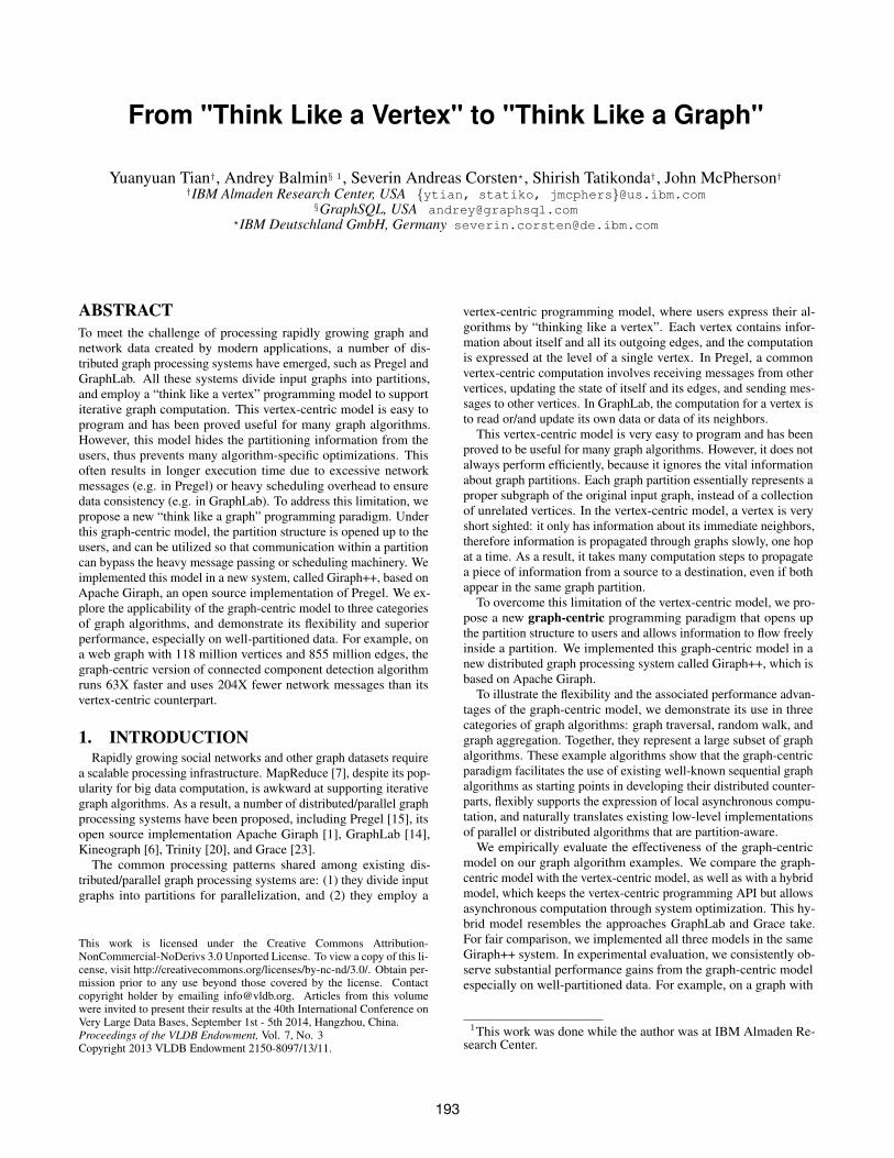
Figure 1: Example graph and graph partitions

118 million vertices and 855 million edges, the graph-centric con-nected component algorithm ran 63X faster than the vertex-centricimplementation and used 204X fewer network messages. This wasalso 27X faster than the hybrid model, even though it used only 2.3Xfewer network messages. These performance gains are due to analgorithm-specific data structure that keeps track of the connectedcomponents within a partition and efficiently merges componentsthat turn out to be connected by a path through other partitions. As aresult, the graph-centric version needs much fewer messages per iter-ation and completes in fewer iterations than both the vertex-centricand the hybrid versions.

Note that the proposed graph-centric programming model is notintended to replace the existing vertex-centric model. Both modelscan be implemented in the same system as we demonstrated inGiraph++. The vertex-centric model has its simplicity. However,the graph-centric model allows lower level access, often needed toimplement important algorithm-specific optimizations. At the sametime, the graph-centric model still provides sufficiently high level ofabstraction and is much easier to use than, for example, MPI[18].

The graph-centric programming model can also be implementedin other graph processing systems. We chose Giraph, due to itspopularity in the open source community, and more importantly itsability to handle graph mutation. Graph mutation is a crucial require-ment for many graph algorithms, especially for graph aggregationalgorithms, such as graph coarsening [12, 11], graph sparsifica-tion [19], and graph summarization [22]. Incidentally, to the bestof our knowledge, Giraph++ is the first system able to support bothasynchronous computation and mutation of graph structures.

The performance of many graph algorithms, especially the onesimplemented in the graph-centric model, can significantly benefitfrom a good graph partitioning strategy that reduces the numberof cross-partition edges. Although there has been a lot of work onsingle-node sequential/parallel graph partitioning algorithms [12,11, 21], the rapid growth of graph data demands scalable distributedgraph partitioning solutions. In this paper, we adapted and extendedthe algorithm of [11] into a distributed graph partitioning algorithm,which we implemented in the same Giraph++ system, using thegraph-centric model.

The remainder of the paper is organized as follows: Section 2provides a necessary background on Giraph. In Section 3, weintroduce the graph-centric programming model, and in Section 4,we exploit the graph-centric model in various graph algorithms. InSection 5, we discuss the hybrid model which is an alternative designto support asynchronous graph computation. Then, the detailedempirical study is provided in Section 6. Section 7 describes therelated work. Finally, we conclude in Section 8.

2. GIRAPH/PREGEL OVERVIEW

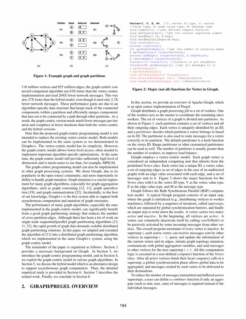
Vertex<I, V, E, M> //I: vertex ID type, V: vertex//value type, E: edge value type, M: message typevoid compute(); //user defined compute functionlong getSuperstep(); //get the current superstep numbervoid sendMsg(I id, M msg);void sendMsgToAllEdges(M msg);void voteToHalt();boolean isHalted();int getNumOutEdges(); //get the number of outgoing edgesE getEdgeValue(I targetVertexId);boolean addEdge(I targetVertexId, E edgeValue);E removeEdge(I targetVertexId);Iterator<I> iterator(); //iterator to all neighborsIterable<M> getMessages(); //get all messages to itI getVertexId();V getVertexValue();void setVertexValue(V vertexValue);void write(DataOutput out); //serializationvoid readFields(DataInput in); //deserialization

Figure 2: Major (not all) functions for Vertex in Giraph.

In this section, we provide an overview of Apache Giraph, whichis an open source implementation of Pregel.

Giraph distributes a graph processing job to a set of workers. Oneof the workers acts as the master to coordinate the remaining slaveworkers. The set of vertices of a graph is divided into partitions. Asshown in Figure 1, each partition contains a set of vertices and alltheir outgoing edges. Each vertex is uniquely identified by an ID,and a partitioner decides which partition a vertex belongs to basedon its ID. The partitioner is also used to route messages for a vertexcorrectly to its partition. The default partitioner is a hash functionon the vertex ID. Range partitioner or other customized partitionerscan be used as well. The number of partitions is usually greater thanthe number of workers, to improve load balance.

Giraph employs a vertex-centric model. Each graph vertex isconsidered an independent computing unit that inherits from thepredefined Vertex class. Each vertex has a unique ID, a vertex value,a set of outgoing edges (a set of edges in the case of an undirectedgraph) with an edge value associated with each edge, and a set ofmessages sent to it. Figure 2 shows the major functions for theVertex class with I as the vertex ID type, V as the vertex value type,E as the edge value type, and M as the message type.

Giraph follows the Bulk Synchronous Parallel (BSP) computa-tion model. A typical Giraph program consists of an input step,where the graph is initialized (e.g., distributing vertices to workermachines), followed by a sequence of iterations, called supersteps,which are separated by global synchronization barriers, and finallyan output step to write down the results. A vertex carries two states:active and inactive. In the beginning, all vertices are active. Avertex can voluntarily deactivate itself by calling voteToHalt() orbe passively activated by some incoming messages from other ver-tices. The overall program terminates if every vertex is inactive. Insuperstep i, each active vertex can receive messages sent by othervertices in superstep i − 1, query and update the information ofthe current vertex and its edges, initiate graph topology mutation,communicate with global aggregation variables, and send messagesto other vertices for the next superstep i+ 1. All this computationlogic is executed in a user-defined compute() function of the Vertexclass. After all active vertices finish their local compute() calls in asuperstep, a global synchronization phase allows global data to beaggregated, and messages created by each vertex to be delivered totheir destinations.

To reduce the number of messages transmitted and buffered acrosssupersteps, a user can define a combiner function if only an aggre-gate (such as min, max, sum) of messages is required instead of theindividual messages.

194

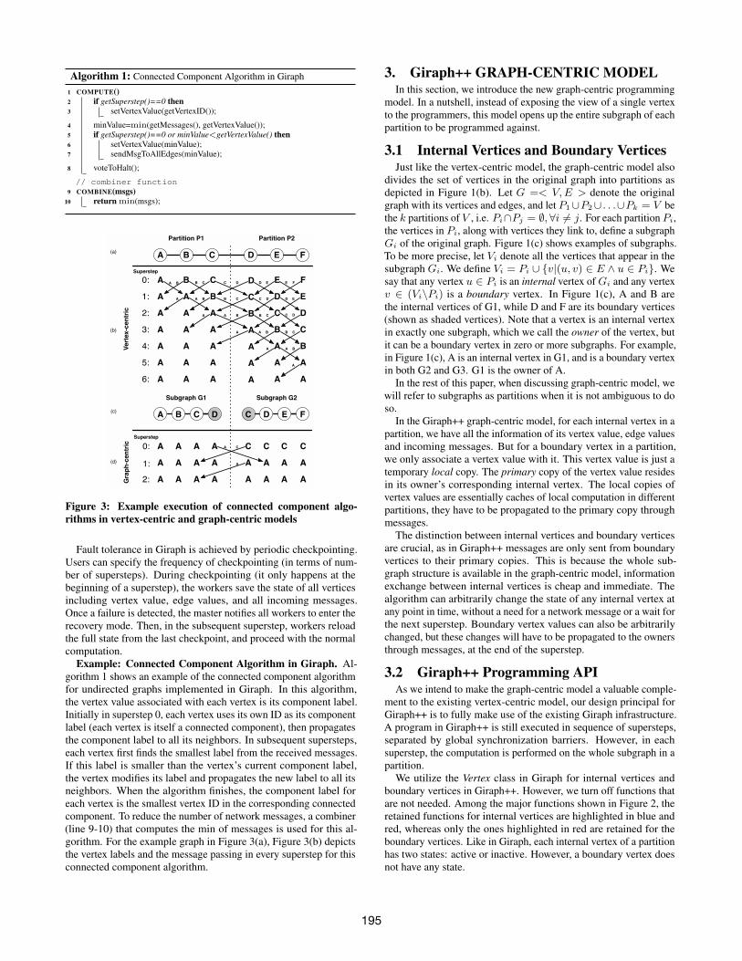
Algorithm 1: Connected Component Algorithm in Giraph

1 COMPUTE()2 if getSuperstep()==0 then3 setVertexValue(getVertexID());

4 minValue=min(getMessages(), getVertexValue());5 if getSuperstep()==0 or minValue<getVertexValue() then6 setVertexValue(minValue);7 sendMsgToAllEdges(minValue);

8 voteToHalt();

// combiner function9 COMBINE(msgs)

10 return min(msgs);

A B C FD E

A B B C C D D E E F

A B B C

A B

A B

A B

B C

C D D E

C D

B C

A

A

A

A

A

A A A C C C

A A A A A A

A A A A A A

A C

A

Vertex-centric

Graph-centric

Superstep

0:

1:

2:

3:

4:

5:

6:

Superstep

0:

1:

2:

(a)

(b)

(d)

A B C D E F

A A C D E

A A A B C D

A A A A B C

A A A A A B

A A A A A A

A A A A A A

Partition P1 Partition P2

B

Subgraph G1 Subgraph G2

A B C D C D E F

A

A

A

(c)

C

A

A

Figure 3: Example execution of connected component algo-rithms in vertex-centric and graph-centric models

Fault tolerance in Giraph is achieved by periodic checkpointing.Users can specify the frequency of checkpointing (in terms of num-ber of supersteps). During checkpointing (it only happens at thebeginning of a superstep), the workers save the state of all verticesincluding vertex value, edge values, and all incoming messages.Once a failure is detected, the master notifies all workers to enter therecovery mode. Then, in the subsequent superstep, workers reloadthe full state from the last checkpoint, and proceed with the normalcomputation.

Example: Connected Component Algorithm in Giraph. Al-gorithm 1 shows an example of the connected component algorithmfor undirected graphs implemented in Giraph. In this algorithm,the vertex value associated with each vertex is its component label.Initially in superstep 0, each vertex uses its own ID as its componentlabel (each vertex is itself a connected component), then propagatesthe component label to all its neighbors. In subsequent supersteps,each vertex first finds the smallest label from the received messages.If this label is smaller than the vertex’s current component label,the vertex modifies its label and propagates the new label to all itsneighbors. When the algorithm finishes, the component label foreach vertex is the smallest vertex ID in the corresponding connectedcomponent. To reduce the number of network messages, a combiner(line 9-10) that computes the min of messages is used for this al-gorithm. For the example graph in Figure 3(a), Figure 3(b) depictsthe vertex labels and the message passing in every superstep for thisconnected component algorithm.

3. Giraph++ GRAPH-CENTRIC MODELIn this section, we introduce the new graph-centric programming

model. In a nutshell, instead of exposing the view of a single vertexto the programmers, this model opens up the entire subgraph of eachpartition to be programmed against.

3.1 Internal Vertices and Boundary VerticesJust like the vertex-centric model, the graph-centric model also

divides the set of vertices in the original graph into partitions asdepicted in Figure 1(b). Let G =< V,E > denote the originalgraph with its vertices and edges, and let P1∪P2∪ . . .∪Pk = V bethe k partitions of V , i.e. Pi∩Pj = ∅,∀i 6= j. For each partition Pi,the vertices in Pi, along with vertices they link to, define a subgraphGi of the original graph. Figure 1(c) shows examples of subgraphs.To be more precise, let Vi denote all the vertices that appear in thesubgraph Gi. We define Vi = Pi ∪ {v|(u, v) ∈ E ∧ u ∈ Pi}. Wesay that any vertex u ∈ Pi is an internal vertex of Gi and any vertexv ∈ (Vi\Pi) is a boundary vertex. In Figure 1(c), A and B arethe internal vertices of G1, while D and F are its boundary vertices(shown as shaded vertices). Note that a vertex is an internal vertexin exactly one subgraph, which we call the owner of the vertex, butit can be a boundary vertex in zero or more subgraphs. For example,in Figure 1(c), A is an internal vertex in G1, and is a boundary vertexin both G2 and G3. G1 is the owner of A.

In the rest of this paper, when discussing graph-centric model, wewill refer to subgraphs as partitions when it is not ambiguous to doso.

In the Giraph++ graph-centric model, for each internal vertex in apartition, we have all the information of its vertex value, edge valuesand incoming messages. But for a boundary vertex in a partition,we only associate a vertex value with it. This vertex value is just atemporary local copy. The primary copy of the vertex value residesin its owner’s corresponding internal vertex. The local copies ofvertex values are essentially caches of local computation in differentpartitions, they have to be propagated to the primary copy throughmessages.

The distinction between internal vertices and boundary verticesare crucial, as in Giraph++ messages are only sent from boundaryvertices to their primary copies. This is because the whole sub-graph structure is available in the graph-centric model, informationexchange between internal vertices is cheap and immediate. Thealgorithm can arbitrarily change the state of any internal vertex atany point in time, without a need for a network message or a wait forthe next superstep. Boundary vertex values can also be arbitrarilychanged, but these changes will have to be propagated to the ownersthrough messages, at the end of the superstep.

3.2 Giraph++ Programming APIAs we intend to make the graph-centric model a valuable comple-

ment to the existing vertex-centric model, our design principal forGiraph++ is to fully make use of the existing Giraph infrastructure.A program in Giraph++ is still executed in sequence of supersteps,separated by global synchronization barriers. However, in eachsuperstep, the computation is performed on the whole subgraph in apartition.

We utilize the Vertex class in Giraph for internal vertices andboundary vertices in Giraph++. However, we turn off functions thatare not needed. Among the major functions shown in Figure 2, theretained functions for internal vertices are highlighted in blue andred, whereas only the ones highlighted in red are retained for theboundary vertices. Like in Giraph, each internal vertex of a partitionhas two states: active or inactive. However, a boundary vertex doesnot have any state.

195

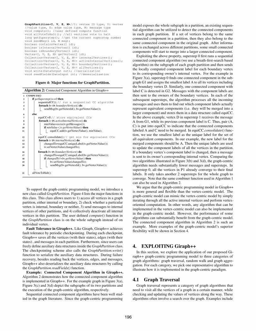
GraphPartition<I, V, E, M>//I: vertex ID type, V: vertex//value type, E: edge value type, M: message typevoid compute(); //user defined compute functionvoid allVoteToHalt(); //all vertices vote to haltlong getSuperstep(); //get the current superstep numbervoid sendMsg(I id, M msg);boolean containsVertex(I id);boolean isInternalVertex(I id);boolean isBoundaryVertex(I id);Vertex<I, V, E, M> getVertex(I id);Collection<Vertex<I, V, E, M>> internalVertices();Collection<Vertex<I, V, E, M>> activeInternalVertices();Collection<Vertex<I, V, E, M>> boundaryVertices();Collection<Vertex<I, V, E, M>> allVertices();void write(DataOutput out); //serializationvoid readFields(DataInput in); //deserialization

Figure 4: Major functions for GraphPartition.

Algorithm 2: Connected Component Algorithm in Giraph++

1 COMPUTE()2 if getSuperstep()==0 then3 sequentialCC(); // run a sequential CC algorithm4 foreach bv IN boundaryVertices() do5 sendMsg(bv.getVertexId(), bv.getVertexValue());

6 else7 equiCC=∅;// store equivalent CCs8 foreach iv IN activeInternalVertices() do9 minValue=min(iv.getMessages());

10 if minValue<iv.getVertexValue() then11 equiCC.add(iv.getVertexValue(), minValue);

12 equiCC.consolidate();// get min for equivalent CCs13 foreach iv IN internalVertices() do14 changedTo=equiCC.uniqueLabel(iv.getVertexValue());15 iv.setVertexValue(changedTo);

16 foreach bv IN boundaryVertices() do17 changedTo=equiCC.uniqueLabel(bv.getVertexValue());18 if changedTo!=bv.getVertexValue() then19 bv.setVertexValue(changedTo);20 sendMsg(bv.getVertexId(), bv.getVertexValue());

21 allVoteToHalt();

To support the graph-centric programming model, we introduce anew class called GraphPartition. Figure 4 lists the major functions inthis class. This class allows users to 1) access all vertices in a graphpartition, either internal or boundary, 2) check whether a particularvertex is internal, boundary or neither, 3) send messages to internalvertices of other partitions, and 4) collectively deactivate all internalvertices in this partition. The user defined compute() function inthe GraphPartition class is on the whole subgraph instead of onindividual vertex.

Fault Tolerance in Giraph++. Like Giraph, Giraph++ achievesfault tolerance by periodic checkpointing. During each checkpoint,Giraph++ saves all the vertices (with their states), edges (with theirstates) , and messages in each partition. Furthermore, since users canfreely define auxiliary data structures inside the GraphPartition class.The checkpointing scheme also calls the GraphPartition.write()function to serialize the auxiliary data structures. During failurerecovery, besides reading back the vertices, edges, and messages,Giraph++ also deserializes the auxiliary data structures by callingthe GraphPartition.readFields() function.

Example: Connected Component Algorithm in Giraph++.Algorithm 2 demonstrates how the connected component algorithmis implemented in Giraph++. For the example graph in Figure 3(a),Figure 3(c) and 3(d) depict the subgraphs of its two partitions andthe execution of the graph-centric algorithm, respectively.

Sequential connected component algorithms have been well stud-ied in the graph literature. Since the graph-centric programming

model exposes the whole subgraph in a partition, an existing sequen-tial algorithm can be utilized to detect the connected componentsin each graph partition. If a set of vertices belong to the sameconnected component in a partition, then they also belong to thesame connected component in the original graph. After informa-tion is exchanged across different partitions, some small connectedcomponents will start to merge into a larger connected component.

Exploiting the above property, superstep 0 first runs a sequentialconnected component algorithm (we use a breath-first-search basedalgorithm) on the subgraph of each graph partition and then sendsthe locally computed component label for each boundary vertexto its corresponding owner’s internal vertex. For the example inFigure 3(a), superstep 0 finds one connected component in the sub-graph G1 and assigns the smallest label A to all its vertices includingthe boundary vertex D. Similarly, one connected component withlabel C is detected in G2. Messages with the component labels arethen sent to the owners of the boundary vertices. In each of thesubsequent supersteps, the algorithm processes all the incomingmessages and uses them to find out which component labels actuallyrepresent equivalent components (i.e. they will be merged into alarger component) and stores them in a data structure called equiCC.In the above example, vertex D in superstep 1 receives the messageA from G1, while its previous component label is C. Thus, pair (A,C) is put into equiCC to indicate that the connected componentslabeled A and C need to be merged. In equiCC.consolidate() func-tion, we use the smallest label as the unique label for the set ofall equivalent components. In our example, the new label for themerged components should be A. Then the unique labels are usedto update the component labels of all the vertices in the partition.If a boundary vertex’s component label is changed, then a messageis sent to its owner’s corresponding internal vertex. Comparing thetwo algorithms illustrated in Figure 3(b) and 3(d), the graph-centricalgorithm needs substantially fewer messages and supersteps. Insuperstep 0, all the vertices in P1 already converge to their finallabels. It only takes another 2 supersteps for the whole graph toconverge. Note that the same combiner function used in Algorithm 1can also be used in Algorithm 2.

We argue that the graph-centric programming model in Giraph++is more general and flexible than the vertex-centric model. Thegraph-centric model can mimic the vertex-centric model by simplyiterating through all the active internal vertices and perform vertex-oriented computation. In other words, any algorithm that can beimplemented in the vertex-centric model can also be implementedin the graph-centric model. However, the performance of somealgorithms can substantially benefit from the graph-centric model.The connected component algorithm in Algorithm 2 is such anexample. More examples of the graph-centric model’s superiorflexibility will be shown in Section 4.

4. EXPLOITING Giraph++In this section, we explore the application of our proposed Gi-

raph++ graph-centric programming model to three categories ofgraph algorithms: graph traversal, random walk and graph aggre-gation. For each category, we pick one representative algorithm toillustrate how it is implemented in the graph-centric paradigm.

4.1 Graph TraversalGraph traversal represents a category of graph algorithms that

need to visit all the vertices of a graph in a certain manner, whilechecking and updating the values of vertices along the way. Thesealgorithms often involve a search over the graph. Examples include

196

Algorithm 3: PageRank Algorithm in Giraph

1 COMPUTE()2 if getSuperstep()≤ MAX ITERATION then3 delta=0;4 if getSuperstep()==0 then5 setVertexValue(0);6 delta+=0.15;

7 delta+=sum(getMessages());8 if delta>0 then9 setVertexValue(getVertexValue()+delta);

10 sendMsgToAllEdges(0.85*delta/getNumOutEdges());

11 voteToHalt();

// combiner function12 COMBINE(msgs)13 return sum(msgs);

computing shortest distances, connected components, transitive clo-sures, etc. Many such algorithms are well-studied, with sequentialimplementations readily available in textbooks and online resources.

We just examined the implementation of one such algorithm in thevertex-centric and the graph-centric models, in Algorithms 1 and 2,respectively. In the graph-centric model, we applied an existingsequential algorithm to the local subgraph of each partition in super-step 0, then only propagate messages through the boundary vertices.In the subsequent supersteps, messages to each vertex could result inthe value update of multiple vertices, thus requiring fewer superstepsthan a corresponding vertex-centric implementation.

4.2 Random WalkThe algorithms of the second category are all based on the ran-

dom walk model. This category includes algorithms like HITS [13],PageRank [5], and its variations, such as ObjectRank [2]. In thissection, we use PageRank as the representative random walk algo-rithm.

Algorithm 3 shows the pseudo code of the PageRank algorithm(using damping factor 0.85) implemented in the vertex-centric model.This is not the classic PageRank implementation, which iterativelyupdates the PageRank based on the values from the previous itera-tion as in PRi

v = d×∑{u|(u,v)∈E}

PRi−1

|Eu| +(1−d), where |Eu|is the number of outgoing edges of u. Instead, Algorithm 3 followsthe accumulative iterative update approach proposed in [25], andincrementally accumulates the intermediate updates to an existingPageRank. It has been proved in [25] that this accumulative updateapproach converges to the same values as the classic PageRankalgorithm. One advantage of this incremental implementation ofPageRank is the ability to update increment values asynchronously,which we will leverage in the graph-centric model below.

Algorithm 4 shows the PageRank algorithm implemented in thegraph-centric model. This algorithm also follows the accumulativeupdate approach. However, there are two crucial differences: (1)Besides the PageRank score, the value of each vertex contains anextra attribute, delta, which caches the intermediate updates re-ceived from other vertices in the same partition (line 16-18). (2)Local PageRank computation is asynchronous, as it utilizes thepartial results of other vertices from the same superstep (line 14).Asynchrony has been demonstrated to accelerate the convergence ofiterative computation in many cases [8], including PageRank [14].Our graph-centric programming paradigm allows the local asyn-chrony to be naturally expressed in the algorithm. Note that boththe vertex-centric and the graph-centric algorithms can benefit froma combiner that computes the sum of all messages (line 12-13 ofAlgorithm 3).

Algorithm 4: PageRank Algorithm in Giraph++

1 COMPUTE()2 if getSuperstep()>MAX ITERATION then3 allVoteToHalt();4 else5 if getSuperstep()==0 then6 foreach v IN allVertices() do7 v.getVertexValue().pr=0;8 v.getVertexValue().delta=0;

9 foreach iv IN activeInternalVertices() do10 if getSuperstep()==0 then11 iv.getVertexValue().delta+=0.15;

12 iv.getVertexValue().delta+=sum(iv.getMessages());13 if iv.getVertexValue().delta>0 then14 iv.getVertexValue().pr+=iv.getVertexValue().delta;15 update=0.85*iv.getVertexValue().delta/iv.getNumOutEdges();

16 while iv.iterator().hashNext() do17 neighbor=getVertex(iv.iterator().next());18 neighbor.getVertexValue().delta+=update;

19 iv.getVertexValue().delta=0;

20 foreach bv IN boundaryVertices() do21 if bv.getVertexValue().delta>0 then22 sendMsg(bv.getVertexId(), bv.getVertexValue().delta);23 bv.getVertexValue().delta=0;

A B

E F

C D

AB

CE DF

w = 2

w = 2 w = 2

w = 2 w = 3

w = 1

(a) (b)

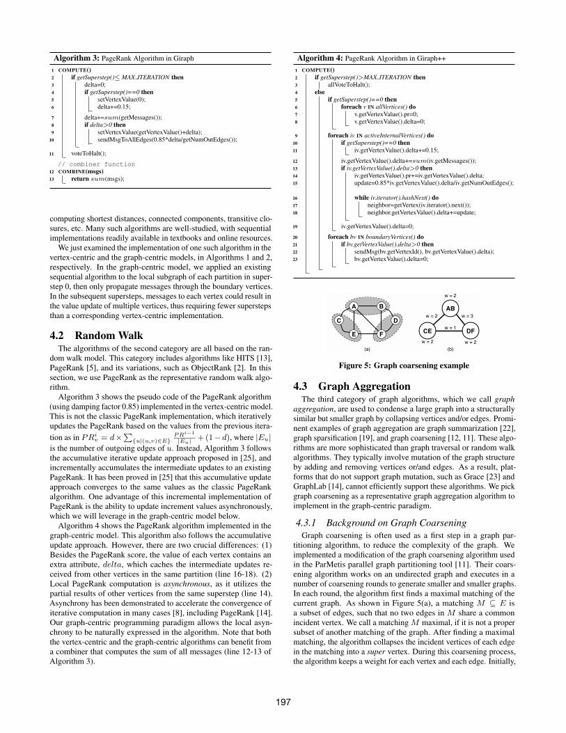
Figure 5: Graph coarsening example

4.3 Graph AggregationThe third category of graph algorithms, which we call graph

aggregation, are used to condense a large graph into a structurallysimilar but smaller graph by collapsing vertices and/or edges. Promi-nent examples of graph aggregation are graph summarization [22],graph sparsification [19], and graph coarsening [12, 11]. These algo-rithms are more sophisticated than graph traversal or random walkalgorithms. They typically involve mutation of the graph structureby adding and removing vertices or/and edges. As a result, plat-forms that do not support graph mutation, such as Grace [23] andGraphLab [14], cannot efficiently support these algorithms. We pickgraph coarsening as a representative graph aggregation algorithm toimplement in the graph-centric paradigm.

4.3.1 Background on Graph CoarseningGraph coarsening is often used as a first step in a graph par-

titioning algorithm, to reduce the complexity of the graph. Weimplemented a modification of the graph coarsening algorithm usedin the ParMetis parallel graph partitioning tool [11]. Their coars-ening algorithm works on an undirected graph and executes in anumber of coarsening rounds to generate smaller and smaller graphs.In each round, the algorithm first finds a maximal matching of thecurrent graph. As shown in Figure 5(a), a matching M ⊆ E isa subset of edges, such that no two edges in M share a commonincident vertex. We call a matching M maximal, if it is not a propersubset of another matching of the graph. After finding a maximalmatching, the algorithm collapses the incident vertices of each edgein the matching into a super vertex. During this coarsening process,the algorithm keeps a weight for each vertex and each edge. Initially,

197

the weights are all 1. The weight of a super vertex is the sum of theweights of all vertices collapsed into it. An edge between two supervertices is an aggregation of edges between the original vertices, soits weight is the sum of the individual edge weights. Figure 5(b)demonstrates an example coarsened graph of Figure 5(a).

In ParMetis [11], finding a maximal matching is done in a numberof phases. In phase i, a processor randomly iterates through its localunmatched vertices. For each such vertex u, it uses a heavy-edgeheuristic to match u with another unmatched vertex v if there is any.If v is local, the match is established immediately. Otherwise, amatch request is sent to the processor that owns v, conditioned uponthe order of u and v: if i is even, a match request is sent only whenu < v; otherwise, a request is sent only when u > v. This orderingconstraint is used to avoid conflicts when both incident vertices ofan edge try to match to each other in the same communication step.In phase i+ 1, multiple match requests for a vertex v is resolved bybreaking conflicts arbitrarily. If a match request from u is granted, anotification is sent back to u. This matching process finishes whena large fraction of vertices are matched.

4.3.2 Graph Coarsening in Giraph++The graph coarsening algorithm in ParMetis can be naturally

implemented in the graph-centric programming model. The (super)vertex during the coarsening process is represented by the Vertexclass in Giraph++. When two (super) vertices are collapsed together,we always reuse one of the (super) vertices. In other words, wemerge one of the vertex into the other. After a merge, however, wedo not delete the vertex that has been merged. We delete all itsedges and declare it inactive, but utilize its vertex value to rememberwhich vertex it has been merged to.

Algorithm Overview. The graph coarsening implementation inour graph-centric model follows the similar process as in the par-allel ParMetis algorithm: The algorithm executes iteratively in asequence of coarsening rounds. Each coarsening round consists ofm matching phases followed by a collapsing phase. Each of thematching phases is completed by 2 supersteps and the collapsingphase corresponds to a single superstep. We empirically observedthat m = 4 is a good number to ensure that a large fraction of thevertices are matched in each coarsening round. Instead of follow-ing exactly the same procedure as ParMetis, we add an importantextension to the coarsening algorithm to specially handle 1-degreevertices. It has been observed that most real graphs follow powerlaw distribution, which means a large number of vertices have verylow degree. 1-degree vertices can be specially handled to improvethe coarsening rate, by simply merging them into their only neighbor.Once again, this merge is done in two supersteps to resolve conflictsthat arise if two vertices only connect to each other and nothing else.

Vertex Data Structure. The value associated with each vertexconsists of the following four attributes: (1) state keeps track ofwhich state the vertex is currently in. It can take one of the 4 val-ues: NORMAL, MATCHREQUESTED, MERGED and MERGEHOST.NORMAL obviously indicates that the vertex is normal – ready todo any action; MATCHREQUESTED means that the vertex just sentout an match request; MERGED denotes that the vertex is or will bemerged into another vertex; and MERGEHOST means that anothervertex will be merged into this vertex. (2) mergedTo records the id ofthe vertex that this vertex is merged into, so that we can reconstructthe member vertices of a super vertex. This attribute is legitimateonly when state=MERGED. (3) weight keeps track of the weight ofthe (super) vertex during the coarsening process. (4) replacementsstores all the pair of vertex replacements in order to guarantee thecorrectness of graph structure change during a merge. For example,consider a graph where A is connected to B, which in turn links

u wv

u v

match request

(a) (b)

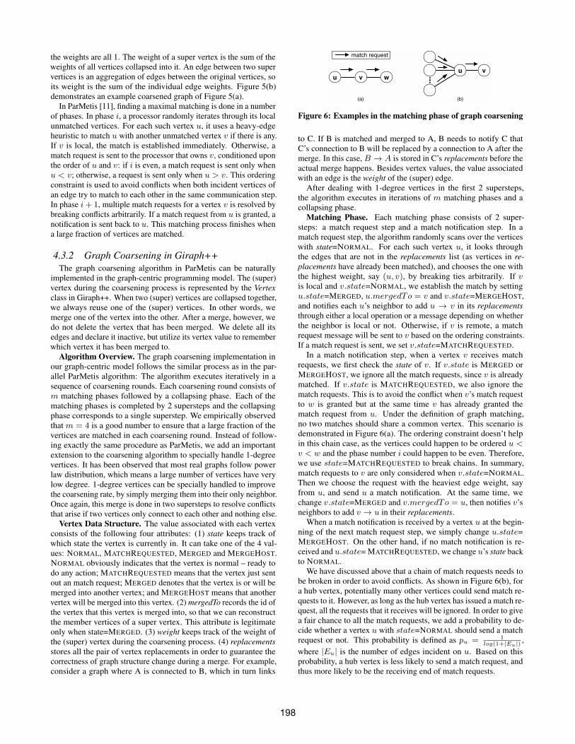
Figure 6: Examples in the matching phase of graph coarsening

to C. If B is matched and merged to A, B needs to notify C thatC’s connection to B will be replaced by a connection to A after themerge. In this case, B → A is stored in C’s replacements before theactual merge happens. Besides vertex values, the value associatedwith an edge is the weight of the (super) edge.

After dealing with 1-degree vertices in the first 2 supersteps,the algorithm executes in iterations of m matching phases and acollapsing phase.

Matching Phase. Each matching phase consists of 2 super-steps: a match request step and a match notification step. In amatch request step, the algorithm randomly scans over the verticeswith state=NORMAL. For each such vertex u, it looks throughthe edges that are not in the replacements list (as vertices in re-placements have already been matched), and chooses the one withthe highest weight, say (u, v), by breaking ties arbitrarily. If vis local and v.state=NORMAL, we establish the match by settingu.state=MERGED, u.mergedTo = v and v.state=MERGEHOST,and notifies each u’s neighbor to add u → v in its replacementsthrough either a local operation or a message depending on whetherthe neighbor is local or not. Otherwise, if v is remote, a matchrequest message will be sent to v based on the ordering constraints.If a match request is sent, we set v.state=MATCHREQUESTED.

In a match notification step, when a vertex v receives matchrequests, we first check the state of v. If v.state is MERGED orMERGEHOST, we ignore all the match requests, since v is alreadymatched. If v.state is MATCHREQUESTED, we also ignore thematch requests. This is to avoid the conflict when v’s match requestto w is granted but at the same time v has already granted thematch request from u. Under the definition of graph matching,no two matches should share a common vertex. This scenario isdemonstrated in Figure 6(a). The ordering constraint doesn’t helpin this chain case, as the vertices could happen to be ordered u <v < w and the phase number i could happen to be even. Therefore,we use state=MATCHREQUESTED to break chains. In summary,match requests to v are only considered when v.state=NORMAL.Then we choose the request with the heaviest edge weight, sayfrom u, and send u a match notification. At the same time, wechange v.state=MERGED and v.mergedTo = u, then notifies v’sneighbors to add v → u in their replacements.

When a match notification is received by a vertex u at the begin-ning of the next match request step, we simply change u.state=MERGEHOST. On the other hand, if no match notification is re-ceived and u.state= MATCHREQUESTED, we change u’s state backto NORMAL.

We have discussed above that a chain of match requests needs tobe broken in order to avoid conflicts. As shown in Figure 6(b), fora hub vertex, potentially many other vertices could send match re-quests to it. However, as long as the hub vertex has issued a match re-quest, all the requests that it receives will be ignored. In order to givea fair chance to all the match requests, we add a probability to de-cide whether a vertex u with state=NORMAL should send a matchrequest or not. This probability is defined as pu = 1

log(1+|Eu|) ,where |Eu| is the number of edges incident on u. Based on thisprobability, a hub vertex is less likely to send a match request, andthus more likely to be the receiving end of match requests.

198

Collapsing Phase. After all the matches are established, in thecollapsing phase, each vertex first processes all the replacementson the edges. After that, if an active vertex u has state=MERGED,it needs to be merged to the target vertex with id=u.mergedTo.If the target vertex is local, the merge is processed immediately.Otherwise, a merge request is sent to the target vertex with u’sweight and all its edges with their weights. Next, we remove all u’sedges but keep u.state and u.mergedTo so that later we can traceback who is merged into whom. After all the merges are done, ifa vertex has state=MERGEHOST, we set it back to NORMAL toparticipate in the next round of coarsening.

5. A HYBRID MODELIn the previous section, we have shown how the graph-centric

model can benefit a number of graph algorithms. One of the ma-jor reasons for the improved performance under the graph-centricmodel is the allowance of the local asynchrony in the computation(e.g. the PageRank algorithm in Algorithm 4): a message sent toa vertex in the same partition can be processed by the receiver inthe same superstep. In addition to using the flexible graph-centricprogramming model, asynchrony can also be achieved by a systemoptimization while keeping the same vertex-centric programmingmodel. We call this approach as the hybrid model.

To implement the hybrid model, we differentiate the messagessent from one partition to the vertices of the same partition, calledinternal messages, from the ones sent to the vertices of a differentpartition, called the external messages. We keep two separate in-coming message buffers for each internal vertex, one for internalmessages called inboxin, and one for the external messages calledinboxex. The external messages are handled using exactly the samemessage passing mechanism as in the vertex-centric model. Anexternal message sent in superstep i can only be seen by the receiverin superstep i+1. In contrast, an internal message is directly placedinto inboxin and can be utilized immediately in the vertex’s com-putation during the same superstep, since both the sender and thereceiver are in the same partition. Suppose vertices A and B are inthe same partition, and during a superstep i, A sends B an internalmessage M. This message is immediately put into B’s inboxin inthe same superstep (with proper locking mechanism to ensure con-sistency). If later B is processed in the same superstep, all messagesin B’s inboxin and inboxex, including M, will be utilized to performB’s compute() function. On the other hand, if B is already processedbefore M is sent in superstep i, then M will be kept in the messagebuffer until B is processed in the next superstep i + 1. To reducethe overhead of maintaining the message buffer, we apply the com-bine() function on the internal messages, whenever a user-definedcombiner is provided.

Under this hybrid model, we can keep exactly the same connectedcomponent algorithm in Algorithm 1 and the PageRank algorithmin Algorithm 3 designed for the vertex-centric model, while stillbenefiting from the asynchronous computation. However, one needsto be cautious when using the hybrid model. First of all, not allgraph problems can benefit from asynchrony. Furthermore, blindlyrunning a vertex-centric algorithm in the hybrid mode is not alwayssafe. For example, the vertex-centric graph coarsening algorithmwon’t work under the hybrid model without change. This is becausethe graph coarsening algorithm requires different types of messagesto be processed at different stages of the computation. The hybridmodel will mix messages from different stages and confuse thecomputation. Even for PageRank, although our specially designedaccumulative iterative update algorithm works without change inthe hybrid model, the classic PageRank algorithm won’t fly in thehybrid model without change. We point out that similar care also

needs to be taken when designing algorithms in other systems thatsupport asynchronous computation.

Note that GraphLab and Grace also allow asynchronous com-putation while keeping the vertex-centric model. Both systemsachieve this goal mainly through the customization of different ver-tex scheduling polices in the systems. However, one price paid forsupporting asynchrony in their systems is that the scheduler can nothandle mutation of graphs. In fact, both GraphLab and Grace re-quire the graph structure to be immutable. This, in turn, limits theirapplicability to any algorithm that mutates the structure of graphs,such as all the graph aggregation algorithms discussed in Section 4.3.In comparison, Giraph++ does not have such conflicts of interests:programmers can freely express the asynchronous computation inthe graph-centric model, while the system maintains the ability tohandle graph mutation.

6. EXPERIMENTAL EVALUATIONIn this section, we empirically compare the performance of the

vertex-centric, the hybrid, and the graph-centric models. For faircomparison among the different models, we implemented all of themin the same Giraph++ system. We refer to these implementations asGiraph++ Vertex Mode (VM), Hybrid Mode (HM), and Graph Mode(GM), respectively. We expect that relative performance trends thatwe observed in this evaluation will hold for other graph processingsystems, though such study is beyond the scope of this paper.

6.1 Experimental SetupWe used four real web graph datasets, shown in Table 1, for

all of our experiments. The first three datasets, uk-2002, uk-2005and webbase-2001 were downloaded from law.di.unimi.it/datasets.php. These datasets were provided by the WebGraph[4] and the LLP [3] projects. The last dataset clueweb50m wasdownloaded from boston.lti.cs.cmu.edu/clueweb09/wiki/tiki-index.php?page=Web+Graph. It is the TREC2009 Category B dataset. All four datasets are directed graphs.Since some algorithms we studied are for undirected graphs, wealso converted the four directed graphs into undirected graphs. Thenumbers of edges in the undirected version of the graphs are shownin the 4th column of Table 1. These four dataset are good rep-resentative for real life graphs with heavy-tail degree distribution.For example, although the uk-2005 graph has an average degree of23.7, the largest in-degree of a vertex is 1,776,852 and the largestout-degree of a vertex is 5,213.

All experiments were conducted on a cluster of 10 IBM Sys-tem x iDataPlex dx340 servers. Each consisted of two quad-coreIntel Xeon E5540 64-bit 2.8GHz processors, 32GB RAM, and in-terconnected using 1Gbit Ethernet. Each server ran Ubuntu Linux(kernel version 2.6.32-24) and Java 1.6. Giraph++ was implementedbased on a version of Apache Giraph downloaded in June 2012,which supports two protocols for message passing: Hadoop RPCand Netty (https://netty.io). We chose Netty (by setting-Dgiraph.useNetty=true), since it proved to be more stable. Eachserver was configured to run up to 6 workers concurrently. Since,a Giraph++ job requires one worker to be the master, there were atmost 59 slave workers running concurrently in the cluster.

Note that in any of the modes, the same algorithm running on thesame input will have some common overhead cost, such as setting upa job, reading the input, shutting down the job, and writing the finaloutput. This overhead stays largely constant in VM, HM, and GM,regardless of the data partitioning strategy. For our largest dataset(webbase-2001), the common overhead is around 113 seconds, 108seconds, and 272 seconds, for connected component, PageRankand graph coarsening, respectively. As many graph algorithms (e.g.

199

directed undirecteddirected undirected partitioning hash partitioned graph partitioned hash partitioned graph partitioned

dataset #nodes #edges #edges #partns time (sec.) ncut imblc ncut imblc ncut imblc ncut imblcuk-2002 18,520,486 298,113,762 261,787,258 177 1,082 0.97 1.01 0.02 2.15 0.99 1.06 0.02 2.24uk-2005 39,459,925 936,364,282 783,027,125 295 6,891 0.98 1.01 0.06 7.39 0.997 1.61 0.06 7.11

webbase-2001 118,142,155 1,019,903,190 854,809,761 826 4,238 0.97 1.03 0.03 3.78 0.999 1.41 0.03 5.05clueweb50m 428,136,613 454,075,604 446,769,872 2891 4,614 0.9997 1.07 0.07 5.56 0.9997 1.96 0.06 6.95

Table 1: Datasets characteristics

PageRank and graph coarsening) requires 100s of supersteps, thiscost is amortized quickly. For example, if we run 100 supersteps forPageRank and graph coarsening, then even for the fastest executiontimes on this dataset (GM with graph partitioning strategy), thecommon overhead accounts for around 7.7% and 8.7% of the totalexecution times, respectively. For the connected component algo-rithm, this cost is more noticeable, however the high-level trends arethe same. Even with overheads included in the execution time, GMis 3X faster than VM on hash partitioned data (instead of 3.1X, ifdiscounting the common overhead) for the connected component al-gorithm. Same speedup on graph partitioned data is 22X (instead of63X, if discounting the common overhead). In order to focus on thedifference in the processing part of VM, HM, and GM, we excludedthe common overhead from the reported execution time for all theexperiments. In addition, except for the experiments in Section 6.6,we turned off the checkpointing to eliminate its overhead.

Exe

cutio

n T

ime

(sec

)

0

10

20

30

40

50

60

Superstep0 5 10 15 20 25 30

VM−HPHM−HPGM−HPVM−GPHM−GPGM−GP

(a) Execution Time

Net

wor

k M

essa

ges

0

1e+008

2e+008

3e+008

4e+008

5e+008

Superstep0 5 10 15 20 25 30

VM−HPHM−HPGM−HPVM−GPHM−GPGM−GP

(b) Network Messages

Figure 7: The execution time and network messages per super-step for connected component detection on uk-2002 dataset.

6.1.1 Scalable Graph PartitioningGraph partitioning plays a crucial role in distributed graph pro-

cessing. For each experiment, we need to first decide on the numberof partitions. Intuitively, a larger partition size would benefit GMand HM, as it increases the chance that neighboring vertices belongto the same partition. However, smaller partitions increase potentialdegree of parallelism and help balance workload across the cluster.We observed empirically that when each partition contained 100,000to 150,000 vertices, all three modes performed well. Therefore, weheuristically set the number of partitions for each graph dataset sothat it is a multiple of 59 (the number of slave workers) and eachpartition contained around 100,000 to 150,000 vertices. The numberof partitions for each dataset used in our experiment is shown incolumn 5 of Table 1.

An even more important question is how to partition a graph. Agood partitioning strategy should minimize the number of edgesthat connect different partitions, to potentially reduce the numberof messages during a distributed computation. Most distributedgraph processing systems, such as Giraph [1] and GraphLab [14],by default use random hash to partition graphs. Obviously, thisrandom partitioning results in a large number of edges crossingpartition boundaries. To quantify this property, we use the well-known Average Normalized Cut measure. Normalized Cut of apartition P , denoted ncut(P), is defined as the faction of edgeslinking vertices in P to vertices in other partitions among all theoutgoing edges of vertices in P, i.e. |{(u,v)∈E|u∈P∧v/∈P}|

|{(u,v)∈E|u∈P}| . Theaverage ncut of all the partitions can be used to measure the qualityof a graph partitioning. As shown in column 7 and column 11 ofTable 1, the average ncuts for hash partitioning across differentdatasets are all very close 1, which means that almost all the edgescross partition boundaries.

GraphLab [14] and the work in [10], also proposed to employthe Metis [12] (sequential) or the ParMetis [11] (parallel) graphpartitioning tools to generate better partitions. However, Metis andParMetis cannot help when the input graph becomes too big to fit inthe memory of a single machine.

We implemented a scalable partitioning approach based on thedistributed graph coarsening algorithm described in Section 4.3.2.This algorithm mimics the parallel multi-level k-way graph parti-tioning algorithm in [11], but is simpler and more scalable. Thereare 3 phases in this algorithm: a coarsening phase, a partitioningphase, and a uncoarsening phase. In the coarsening phase, we ap-ply the distributed graph coarsening algorithm in Section 4.3.2 toreduce the input graph into a manageable size that can fit in a singlemachine. Then, in the partitioning phase, a single node sequentialor parallel graph partitioning algorithm is applied to the coarsenedgraph. We simply use the ParMetis algorithm in this step. At last,in the uncoarsening phase, we project the partitions back to theoriginal graph. This phase does not apply any refinements on thepartitions as in [11]. However, uncoarsening has to be executed in adistributed fashion as well. Recall that in the coarsening phase eachvertex that is merged into another has an attribute called mergedToto keep track of the host of the merger. This attribute can help usderive the membership information for each partition. Suppose thata vertex A is merged into B which in turn is merged into C, andfinally C belongs to a partition P. We can use the mergedTo attributeto form an edge in a membership forest. In this example, we havean edge between A and B, and an edge between B and C. Findingwhich vertices ultimately belong to the partition P is essentiallyfinding the connected components in the membership forest. Thus,we use Algorithm 2 in the last stage of graph partitioning.

Column 6 of Table 1 shows the total graph partitioning time, withgraph coarsening running 100 supersteps in the graph-centric model.The average ncuts of graph partitions produced by this algorithmare listed in columns 9 and 13. On average, only 2% to 7% edgesgo across partitions.

There is another important property of graph partitioning that af-fects the performance of a distributed graph algorithm: load balance.

200

execution time (sec) network messages (millions) number of superstepshash partitioned (HP) graph partitioned (GP) hash partitioned (HP) graph partitioned (GP) hash partitioned (HP) graph partitioned (GP)

dataset VM HM GM VM HM GM VM HM GM VM HM GM VM HM GM VM HM GMuk-2002 441 438 272 532 89 19 3,315 3,129 1,937 3,414 17 8.7 33 32 19 33 19 5uk-2005 1,366 1,354 723 1,700 230 90 11,361 10,185 5,188 10,725 370 225 22 22 16 22 12 5

webbase-2001 4,491 4,405 1,427 3,599 1,565 57 13,348 11,198 6,581 11,819 136 58 605 604 39 605 319 5clueweb50m 1,875 2,103 1,163 1,072 250 103 6,391 5,308 2,703 6,331 129 69 38 37 14 38 18 5

Table 2: Total execution time, network messages, and number of supersteps for connected component detection

For many algorithms, running time for each partition is significantlyaffected by its number of edges. Therefore, we also need to measurehow the edges are distributed across partitions. We define the loadimbalance of a graph partitioning as the maximum number of edgesin a partition divided by the average number of edges per partition,i.e. max(|EP |)×p∑

|EP |, where EP = {(u, v) ∈ E|u ∈ P} and p is

the number of partitions. Table 1 also shows the load imbalancefactors for both hash partitioning and our proposed graph partition-ing across different datasets. Clearly, hash partitioning results inbetter balanced partitions than our graph partitioning method. Thisis because most real graph datasets present a preferential attachmentphenomenon: new edges tend to be established between alreadywell-connected vertices [17]. As a result, a partition that containsa well-connected vertex will naturally bring in much more edgesthan expected. Producing balanced graph partitions with minimalcommunication cost is an NP-hard problem and is a difficult trade-off in practice, especially for very skewed graphs. Newly proposedpartitioning technique with dynamic load balancing [24], and thevertex-cut approach introduced in the latest version of Graphlab [9]can potentially help alleviate the problem, but cannot completelysolve the problem.

We decided to “eat our own dog food” and evaluate the connectedcomponent and PageRank algorithms, using our graph partitioning(GP) strategy in addition to the default hash partitioning (HP). Notethat the focus of this evaluation is on comparing Giraph++ VM,HM, and GM modes. Although we implemented a scalable graphpartitioning algorithm and use its output to evaluate two distributedgraph algorithms, we leave the in-depth study of graph partitioningalgorithms for the future work. The GP experiments should beviewed as a proxy for a scenario where some scalable graph parti-tioning algorithm is used as a part of graph processing pipeline. Thisshould be the case if graphs are analyzed by (multiple) expensivealgorithms, so that the performance benefits of the low ncut justifythe partitioning cost.

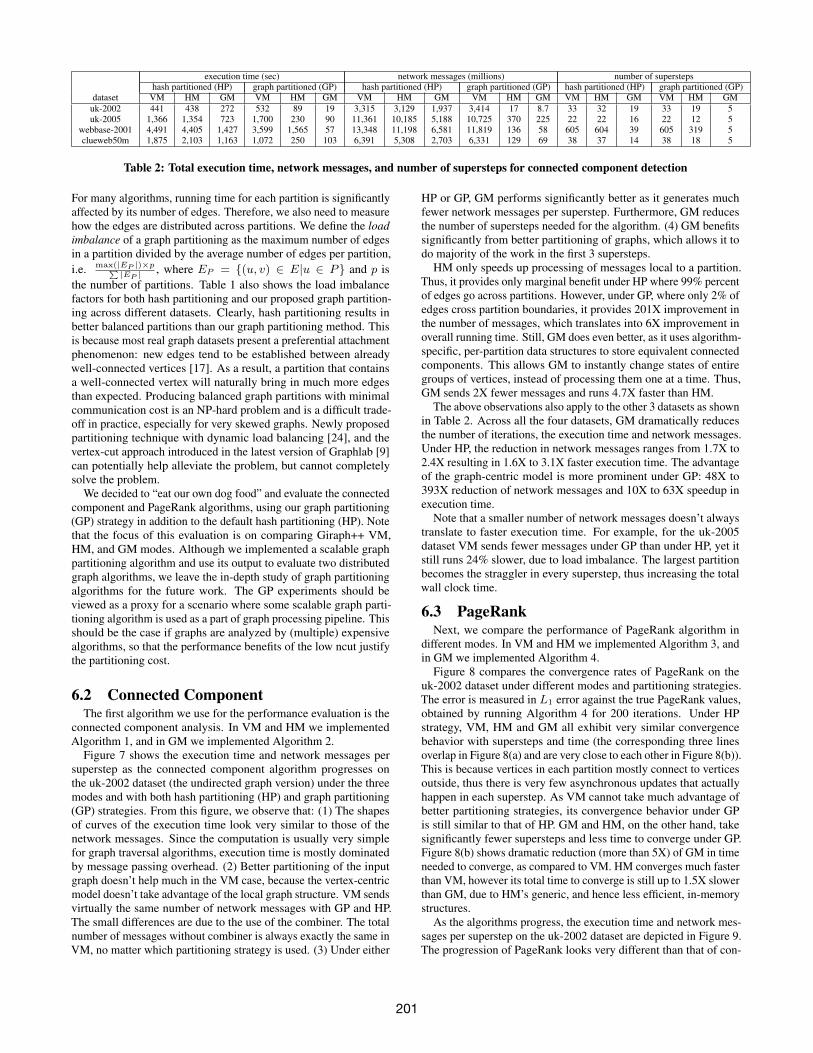
6.2 Connected ComponentThe first algorithm we use for the performance evaluation is the

connected component analysis. In VM and HM we implementedAlgorithm 1, and in GM we implemented Algorithm 2.

Figure 7 shows the execution time and network messages persuperstep as the connected component algorithm progresses onthe uk-2002 dataset (the undirected graph version) under the threemodes and with both hash partitioning (HP) and graph partitioning(GP) strategies. From this figure, we observe that: (1) The shapesof curves of the execution time look very similar to those of thenetwork messages. Since the computation is usually very simplefor graph traversal algorithms, execution time is mostly dominatedby message passing overhead. (2) Better partitioning of the inputgraph doesn’t help much in the VM case, because the vertex-centricmodel doesn’t take advantage of the local graph structure. VM sendsvirtually the same number of network messages with GP and HP.The small differences are due to the use of the combiner. The totalnumber of messages without combiner is always exactly the same inVM, no matter which partitioning strategy is used. (3) Under either

HP or GP, GM performs significantly better as it generates muchfewer network messages per superstep. Furthermore, GM reducesthe number of supersteps needed for the algorithm. (4) GM benefitssignificantly from better partitioning of graphs, which allows it todo majority of the work in the first 3 supersteps.

HM only speeds up processing of messages local to a partition.Thus, it provides only marginal benefit under HP where 99% percentof edges go across partitions. However, under GP, where only 2% ofedges cross partition boundaries, it provides 201X improvement inthe number of messages, which translates into 6X improvement inoverall running time. Still, GM does even better, as it uses algorithm-specific, per-partition data structures to store equivalent connectedcomponents. This allows GM to instantly change states of entiregroups of vertices, instead of processing them one at a time. Thus,GM sends 2X fewer messages and runs 4.7X faster than HM.

The above observations also apply to the other 3 datasets as shownin Table 2. Across all the four datasets, GM dramatically reducesthe number of iterations, the execution time and network messages.Under HP, the reduction in network messages ranges from 1.7X to2.4X resulting in 1.6X to 3.1X faster execution time. The advantageof the graph-centric model is more prominent under GP: 48X to393X reduction of network messages and 10X to 63X speedup inexecution time.

Note that a smaller number of network messages doesn’t alwaystranslate to faster execution time. For example, for the uk-2005dataset VM sends fewer messages under GP than under HP, yet itstill runs 24% slower, due to load imbalance. The largest partitionbecomes the straggler in every superstep, thus increasing the totalwall clock time.

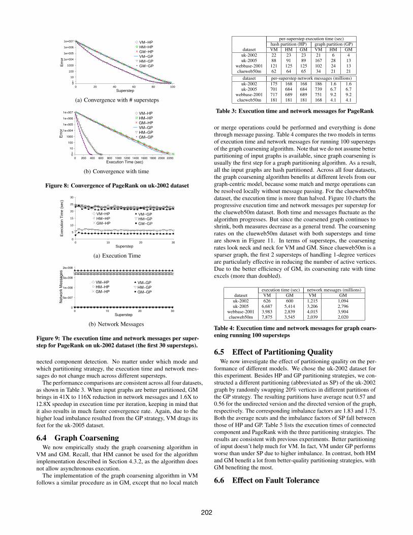
6.3 PageRankNext, we compare the performance of PageRank algorithm in

different modes. In VM and HM we implemented Algorithm 3, andin GM we implemented Algorithm 4.

Figure 8 compares the convergence rates of PageRank on theuk-2002 dataset under different modes and partitioning strategies.The error is measured in L1 error against the true PageRank values,obtained by running Algorithm 4 for 200 iterations. Under HPstrategy, VM, HM and GM all exhibit very similar convergencebehavior with supersteps and time (the corresponding three linesoverlap in Figure 8(a) and are very close to each other in Figure 8(b)).This is because vertices in each partition mostly connect to verticesoutside, thus there is very few asynchronous updates that actuallyhappen in each superstep. As VM cannot take much advantage ofbetter partitioning strategies, its convergence behavior under GPis still similar to that of HP. GM and HM, on the other hand, takesignificantly fewer supersteps and less time to converge under GP.Figure 8(b) shows dramatic reduction (more than 5X) of GM in timeneeded to converge, as compared to VM. HM converges much fasterthan VM, however its total time to converge is still up to 1.5X slowerthan GM, due to HM’s generic, and hence less efficient, in-memorystructures.

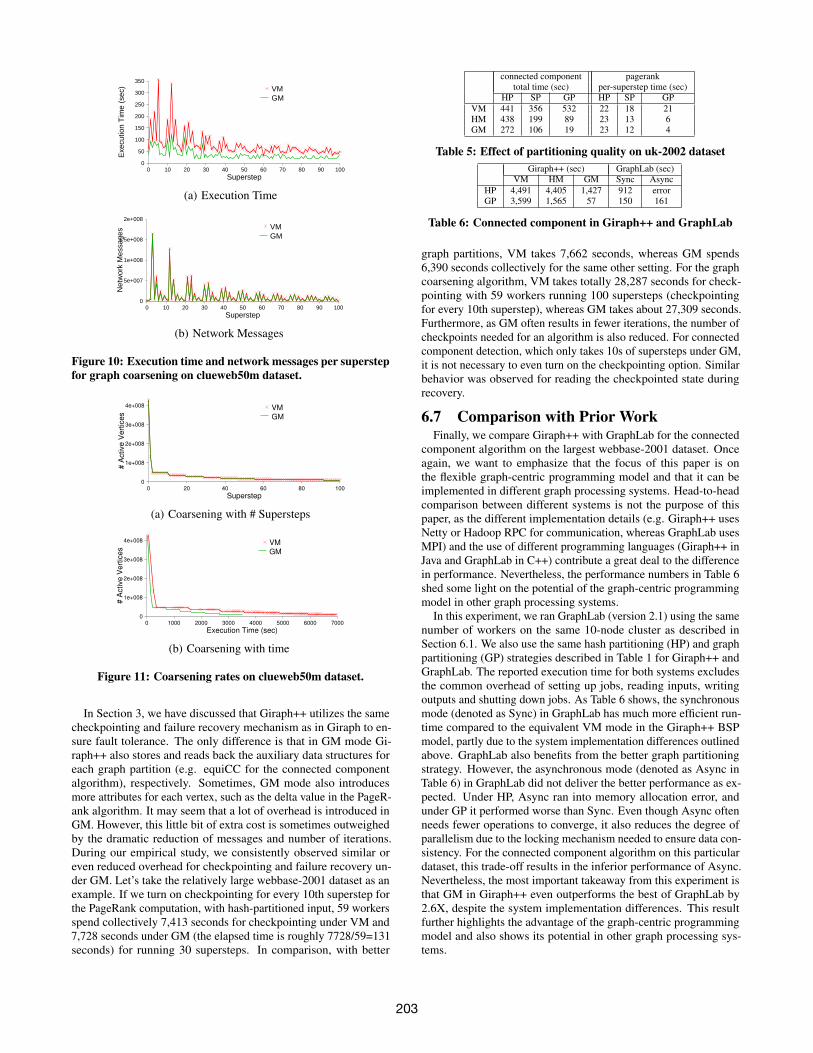
As the algorithms progress, the execution time and network mes-sages per superstep on the uk-2002 dataset are depicted in Figure 9.The progression of PageRank looks very different than that of con-

201

Err

or

1e+007

1e+006

1e+005

1e+004

1000

100

10

10

Superstep0 20 40 60 80 100

VM−HPHM−HPGM−HPVM−GPHM−GPGM−GP

(a) Convergence with # supersteps

Err

or

1e+007

1e+006

1e+005

1e+004

1000

100

10

10

Execution Time (sec)0 200 400 600 800 1000 1200 1400 1600 1800 2000 2200

VM−HP

HM−HP

GM−HP

VM−GP

HM−GP

GM−GP

(b) Convergence with time

Figure 8: Convergence of PageRank on uk-2002 dataset

Exe

cutio

n T

ime

(sec

)

0

5

10

15

20

25

30

Superstep0 10 20 30

VM−HPHM−HPGM−HP

VM−GPHM−GPGM−GP

(a) Execution Time

Ne

two

rk M

essa

ge

s

0

5e+007

1e+008

1.5e+008

2e+008

Superstep0 10 20 30

VM−HP

HM−HP

GM−HP

VM−GP

HM−GP

GM−GP

(b) Network Messages

Figure 9: The execution time and network messages per super-step for PageRank on uk-2002 dataset (the first 30 supersteps).

nected component detection. No matter under which mode andwhich partitioning strategy, the execution time and network mes-sages do not change much across different supersteps.

The performance comparisons are consistent across all four datasets,as shown in Table 3. When input graphs are better partitioned, GMbrings in 41X to 116X reduction in network messages and 1.6X to12.8X speedup in execution time per iteration, keeping in mind thatit also results in much faster convergence rate. Again, due to thehigher load imbalance resulted from the GP strategy, VM drags itsfeet for the uk-2005 dataset.

6.4 Graph CoarseningWe now empirically study the graph coarsening algorithm in

VM and GM. Recall, that HM cannot be used for the algorithmimplementation described in Section 4.3.2, as the algorithm doesnot allow asynchronous execution.

The implementation of the graph coarsening algorithm in VMfollows a similar procedure as in GM, except that no local match

per-superstep execution time (sec)hash partition (HP) graph partition (GP)

dataset VM HM GM VM HM GMuk-2002 22 23 23 21 6 4uk-2005 88 91 89 167 28 13

webbase-2001 121 125 125 102 24 13clueweb50m 62 64 65 34 21 21

dataset per-superstep network messages (millions)uk-2002 175 168 168 186 1.6 1.6uk-2005 701 684 684 739 6.7 6.7

webbase-2001 717 689 689 751 9.2 9.2clueweb50m 181 181 181 168 4.1 4.1

Table 3: Execution time and network messages for PageRank

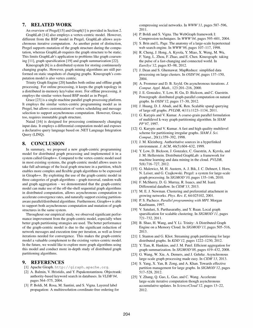
or merge operations could be performed and everything is donethrough message passing. Table 4 compares the two models in termsof execution time and network messages for running 100 superstepsof the graph coarsening algorithm. Note that we do not assume betterpartitioning of input graphs is available, since graph coarsening isusually the first step for a graph partitioning algorithm. As a result,all the input graphs are hash partitioned. Across all four datasets,the graph coarsening algorithm benefits at different levels from ourgraph-centric model, because some match and merge operations canbe resolved locally without message passing. For the clueweb50mdataset, the execution time is more than halved. Figure 10 charts theprogressive execution time and network messages per superstep forthe clueweb50m dataset. Both time and messages fluctuate as thealgorithm progresses. But since the coarsened graph continues toshrink, both measures decrease as a general trend. The coarseningrates on the clueweb50m dataset with both supersteps and timeare shown in Figure 11. In terms of supersteps, the coarseningrates look neck and neck for VM and GM. Since clueweb50m is asparser graph, the first 2 supersteps of handling 1-degree verticesare particularly effective in reducing the number of active vertices.Due to the better efficiency of GM, its coarsening rate with timeexcels (more than doubled).

execution time (sec) network messages (millions)dataset VM GM VM GM

uk-2002 626 600 1,215 1,094uk-2005 6,687 5,414 3,206 2,796

webbase-2001 3,983 2,839 4,015 3,904clueweb50m 7,875 3,545 2,039 2,020

Table 4: Execution time and network messages for graph coars-ening running 100 supersteps

6.5 Effect of Partitioning QualityWe now investigate the effect of partitioning quality on the per-

formance of different models. We chose the uk-2002 dataset forthis experiment. Besides HP and GP partitioning strategies, we con-structed a different partitioning (abbreviated as SP) of the uk-2002graph by randomly swapping 20% vertices in different partitions ofthe GP strategy. The resulting partitions have average ncut 0.57 and0.56 for the undirected version and the directed version of the graph,respectively. The corresponding imbalance factors are 1.83 and 1.75.Both the average ncuts and the imbalance factors of SP fall betweenthose of HP and GP. Table 5 lists the execution times of connectedcomponent and PageRank with the three partitioning strategies. Theresults are consistent with previous experiments. Better partitioningof input doesn’t help much for VM. In fact, VM under GP performsworse than under SP due to higher imbalance. In contrast, both HMand GM benefit a lot from better-quality partitioning strategies, withGM benefiting the most.

6.6 Effect on Fault Tolerance

202

Exe

cutio

n T

ime

(sec

)

0

50

100

150

200

250

300

350

Superstep0 10 20 30 40 50 60 70 80 90 100

VMGM

(a) Execution Time

Net

wor

k M

essa

ges

0

5e+007

1e+008

1.5e+008

2e+008

Superstep0 10 20 30 40 50 60 70 80 90 100

VMGM

(b) Network Messages

Figure 10: Execution time and network messages per superstepfor graph coarsening on clueweb50m dataset.

# A

ctive V

ert

ices

0

1e+008

2e+008

3e+008

4e+008

Superstep0 20 40 60 80 100

VM

GM

(a) Coarsening with # Supersteps

# A

ctive

Ve

rtic

es

0

1e+008

2e+008

3e+008

4e+008

Execution Time (sec)0 1000 2000 3000 4000 5000 6000 7000

VM

GM

(b) Coarsening with time

Figure 11: Coarsening rates on clueweb50m dataset.

In Section 3, we have discussed that Giraph++ utilizes the samecheckpointing and failure recovery mechanism as in Giraph to en-sure fault tolerance. The only difference is that in GM mode Gi-raph++ also stores and reads back the auxiliary data structures foreach graph partition (e.g. equiCC for the connected componentalgorithm), respectively. Sometimes, GM mode also introducesmore attributes for each vertex, such as the delta value in the PageR-ank algorithm. It may seem that a lot of overhead is introduced inGM. However, this little bit of extra cost is sometimes outweighedby the dramatic reduction of messages and number of iterations.During our empirical study, we consistently observed similar oreven reduced overhead for checkpointing and failure recovery un-der GM. Let’s take the relatively large webbase-2001 dataset as anexample. If we turn on checkpointing for every 10th superstep forthe PageRank computation, with hash-partitioned input, 59 workersspend collectively 7,413 seconds for checkpointing under VM and7,728 seconds under GM (the elapsed time is roughly 7728/59=131seconds) for running 30 supersteps. In comparison, with better

connected component pageranktotal time (sec) per-superstep time (sec)

HP SP GP HP SP GPVM 441 356 532 22 18 21HM 438 199 89 23 13 6GM 272 106 19 23 12 4

Table 5: Effect of partitioning quality on uk-2002 datasetGiraph++ (sec) GraphLab (sec)

VM HM GM Sync AsyncHP 4,491 4,405 1,427 912 errorGP 3,599 1,565 57 150 161

Table 6: Connected component in Giraph++ and GraphLab

graph partitions, VM takes 7,662 seconds, whereas GM spends6,390 seconds collectively for the same other setting. For the graphcoarsening algorithm, VM takes totally 28,287 seconds for check-pointing with 59 workers running 100 supersteps (checkpointingfor every 10th superstep), whereas GM takes about 27,309 seconds.Furthermore, as GM often results in fewer iterations, the number ofcheckpoints needed for an algorithm is also reduced. For connectedcomponent detection, which only takes 10s of supersteps under GM,it is not necessary to even turn on the checkpointing option. Similarbehavior was observed for reading the checkpointed state duringrecovery.

6.7 Comparison with Prior WorkFinally, we compare Giraph++ with GraphLab for the connected

component algorithm on the largest webbase-2001 dataset. Onceagain, we want to emphasize that the focus of this paper is onthe flexible graph-centric programming model and that it can beimplemented in different graph processing systems. Head-to-headcomparison between different systems is not the purpose of thispaper, as the different implementation details (e.g. Giraph++ usesNetty or Hadoop RPC for communication, whereas GraphLab usesMPI) and the use of different programming languages (Giraph++ inJava and GraphLab in C++) contribute a great deal to the differencein performance. Nevertheless, the performance numbers in Table 6shed some light on the potential of the graph-centric programmingmodel in other graph processing systems.

In this experiment, we ran GraphLab (version 2.1) using the samenumber of workers on the same 10-node cluster as described inSection 6.1. We also use the same hash partitioning (HP) and graphpartitioning (GP) strategies described in Table 1 for Giraph++ andGraphLab. The reported execution time for both systems excludesthe common overhead of setting up jobs, reading inputs, writingoutputs and shutting down jobs. As Table 6 shows, the synchronousmode (denoted as Sync) in GraphLab has much more efficient run-time compared to the equivalent VM mode in the Giraph++ BSPmodel, partly due to the system implementation differences outlinedabove. GraphLab also benefits from the better graph partitioningstrategy. However, the asynchronous mode (denoted as Async inTable 6) in GraphLab did not deliver the better performance as ex-pected. Under HP, Async ran into memory allocation error, andunder GP it performed worse than Sync. Even though Async oftenneeds fewer operations to converge, it also reduces the degree ofparallelism due to the locking mechanism needed to ensure data con-sistency. For the connected component algorithm on this particulardataset, this trade-off results in the inferior performance of Async.Nevertheless, the most important takeaway from this experiment isthat GM in Giraph++ even outperforms the best of GraphLab by2.6X, despite the system implementation differences. This resultfurther highlights the advantage of the graph-centric programmingmodel and also shows its potential in other graph processing sys-tems.

203

7. RELATED WORKAn overview of Pregel[15] and Giraph[1] is provided in Section 2.GraphLab [14] also employs a vertex-centric model. However,

different from the BSP model in Pregel, GraphLab allows asyn-chronous iterative computation. As another point of distinction,Pregel supports mutation of the graph structure during the compu-tation, whereas GraphLab requires the graph structure to be static.This limits GraphLab’s application to problems like graph coarsen-ing [11], graph sparsification [19] and graph summarization [22].

Kineograph [6] is a distributed system for storing continuouslychanging graphs. However, graph mining algorithms are still per-formed on static snapshots of changing graphs. Kineograph’s com-putation model is also vertex centric.

Trinity Graph Engine [20] handles both online and offline graphprocessing. For online processing, it keeps the graph topology ina distributed in-memory key/value store. For offline processing, itemploys the similar vertex-based BSP model as in Pregel.

Grace [23] is a single-machine parallel graph processing platform.It employs the similar vertex-centric programming model as inPregel, but allows customization of vertex scheduling and messageselection to support asynchronous computation. However, Grace,too, requires immutable graph structure.

Naiad [16] is designed for processing continuously changinginput data. It employs a differential computation model and exposesa declarative query language based on .NET Language IntegrationQuery (LINQ).

8. CONCLUSIONIn summary, we proposed a new graph-centric programming

model for distributed graph processing and implemented it in asystem called Giraph++. Compared to the vertex-centric model usedin most existing systems, the graph-centric model allows users totake full advantage of the local graph structure in a partition, whichenables more complex and flexible graph algorithms to be expressedin Giraph++. By exploiting the use of the graph-centric model inthree categories of graph algorithms – graph traversal, random walkand graph aggregation – we demonstrated that the graph-centricmodel can make use of the off-the-shell sequential graph algorithmsin distributed computation, allows asynchronous computation toaccelerate convergence rates, and naturally support existing partition-aware parallel/distributed algorithms. Furthermore, Giraph++ is ableto support both asynchronous computation and mutation of graphstructures in the same system.

Throughout our empirical study, we observed significant perfor-mance improvement from the graph-centric model, especially whenbetter graph partitioning strategies are used. The better performanceof the graph-centric model is due to the significant reduction ofnetwork messages and execution time per iteration, as well as feweriterations needed for convergence. This makes the graph-centricmodel a valuable complement to the existing vertex-centric model.In the future, we would like to explore more graph algorithms usingthis model and conduct more in-depth study of distributed graphpartitioning algorithms.

9. REFERENCES[1] Apache Giraph. http://giraph.apache.org.[2] A. Balmin, V. Hristidis, and Y. Papakonstantinou. Objectrank:

authority-based keyword search in databases. In VLDB’04,pages 564–575, 2004.

[3] P. Boldi, M. Rosa, M. Santini, and S. Vigna. Layered labelpropagation: A multiresolution coordinate-free ordering for

compressing social networks. In WWW’11, pages 587–596,2011.

[4] P. Boldi and S. Vigna. The WebGraph framework I:Compression techniques. In WWW’04, pages 595–601, 2004.

[5] S. Brin and L. Page. The anatomy of a large-scale hypertextualweb search engine. In WWW’98, pages 107–117, 1998.

[6] R. Cheng, J. Hong, A. Kyrola, Y. Miao, X. Weng, M. Wu,F. Yang, L. Zhou, F. Zhao, and E. Chen. Kineograph: takingthe pulse of a fast-changing and connected world. InEuroSys’12, pages 85–98, 2012.

[7] J. Dean and S. Ghemawat. MapReduce: simplified dataprocessing on large clusters. In OSDI’04, pages 137–150,2004.

[8] A. Frommer and D. B. Szyld. On asynchronous iterations. J.Comput. Appl. Math., 123:201–216, 2000.

[9] J. E. Gonzalez, Y. Low, H. Gu, D. Bickson, and C. Guestrin.Powergraph: distributed graph-parallel computation on naturalgraphs. In OSDI’12, pages 17–30, 2012.

[10] J. Huang, D. J. Abadi, and K. Ren. Scalable sparql queryingof large rdf graphs. PVLDB, 4(11):1123–1134, 2011.

[11] G. Karypis and V. Kumar. A coarse-grain parallel formulationof multilevel k-way graph partitioning algorithm. In SIAMPP’97, 1997.

[12] G. Karypis and V. Kumar. A fast and high quality multilevelscheme for partitioning irregular graphs. SIAM J. Sci.Comput., 20(1):359–392, 1998.

[13] J. M. Kleinberg. Authoritative sources in a hyperlinkedenvironment. J. ACM, 46(5):604–632, 1999.

[14] Y. Low, D. Bickson, J. Gonzalez, C. Guestrin, A. Kyrola, andJ. M. Hellerstein. Distributed GraphLab: a framework formachine learning and data mining in the cloud. PVLDB,5(8):716–727, 2012.

[15] G. Malewicz, M. H. Austern, A. J. Bik, J. C. Dehnert, I. Horn,N. Leiser, and G. Czajkowski. Pregel: a system for large-scalegraph processing. In SIGMOD’10, pages 135–146, 2010.

[16] F. McSherry, D. G. Murray, R. Isaacs, and M. Isard.Differential dataflow. In CIDR’13, 2013.

[17] M. E. J. Newman. Clustering and preferential attachment ingrowing networks. Phys. Rev. E, 64:025102, 2001.

[18] P. S. Pacheco. Parallel programming with MPI. MorganKaufmann, 1997.

[19] V. Satuluri, S. Parthasarathy, and Y. Ruan. Local graphsparsification for scalable clustering. In SIGMOD’11, pages721–732, 2011.

[20] B. Shao, H. Wang, and Y. Li. Trinity: A Distributed GraphEngine on a Memory Cloud. In SIGMOD’13, pages 505–516,2013.

[21] I. Stanton and G. Kliot. Streaming graph partitioning for largedistributed graphs. In KDD’12, pages 1222–1230, 2012.

[22] Y. Tian, R. Hankins, and J. M. Patel. Efficient aggregation forgraph summarization. In SIGMOD’08, pages 419–432, 2008.

[23] G. Wang, W. Xie, A. Demers, and J. Gehrke. Asynchronouslarge-scale graph processing made easy. In CIDR’13, 2013.

[24] S. Yang, X. Yan, B. Zong, and A. Khan. Towards effectivepartition management for large graphs. In SIGMOD’12, pages517–528, 2012.

[25] Y. Zhang, Q. Gao, L. Gao, and C. Wang. Acceleratelarge-scale iterative computation though asynchronousaccumulative updates. In ScienceCloud’12, pages 13–22,2012.

204