from the forest to the faucet - home | us forest service

USDA FOREST SERVICE

From the Forest to the Faucet Drinking Water and Forests in the US

Methods Paper

Emily Weidner & Al Todd

Ecosystem Services & Markets Program Area State and Private Forestry

October 2011

USDA Forest Service October 2011

2

CONTENTS

Tables and Figures ......................................................................................................................................................... 3

Introduction ................................................................................................................................................................... 4

Approach ....................................................................................................................................................................... 5

Scale ............................................................................................................................................................................... 7

Step One: Important Areas for Surface Drinking Water ............................................................................................... 8

Overview .................................................................................................................................................................... 8

Drinking Water Protection Model, PR ....................................................................................................................... 8

A Special Case: The Great Lakes Region ................................................................................................................. 12

Mean Annual Water Supply, Q ................................................................................................................................ 14

The Final Model: Index of Importance to Surface Drinking Water, IMP ................................................................. 15

Step Two: Forest Importance to Surface Drinking Water ............................................................................................ 16

Step Three: Threats to Forests Important for Surface Drinking Water ...................................................................... 20

Overview .................................................................................................................................................................. 20

Increased Housing Density ...................................................................................................................................... 21

Insect and Disease Risk ............................................................................................................................................ 23

Wildfire Risk ............................................................................................................................................................. 24

Applications ................................................................................................................................................................. 27

Introduction ............................................................................................................................................................. 27

Potential Sites for Payment for Watershed Services ............................................................................................... 27

Spatial Decision Support Tools ................................................................................................................................ 27

Acknowledgements ..................................................................................................................................................... 29

Correspondence .......................................................................................................................................................... 29

References ................................................................................................................................................................... 30

Appendix 1: Data Readme File .................................................................................................................................... 32

Appendix 2: EPA Safe Drinking Water Information System (SDWIS) .......................................................................... 33


3

TABLES AND FIGURES

Table 1. Proportional weights for each upstream sub-watershed ............................................................................. 12 Figure 1. Conceptual model for the analysis process. ................................................................................................... 5

Figure 2. Surface drinking water protection model, PR. ............................................................................................ 10

Figure 3. Schematic of surface drinking water protection model, PR. ....................................................................... 11

Figure 4. Expontial decay relationship between distance from intake, d, and the proportional weight, W. .............. 11

Figure 5. PR values for the Great Lakes Region. ......................................................................................................... 13

Figure 6. Mean annual water supply, Q. ...................................................................................................................... 14

Figure 7. Surface drinking water importance index, IMP. ........................................................................................... 15

Figure 8. Percent any forest land, private forests, protected forest, and, NFS land in each sub-watershed. . ........... 17

Figure 9. The index of forest importance to surface drinking water. ......................................................................... 18

Figure 10. The index of private forest importance to surface drinking water. ........................................................... 18

Figure 11. The index of protected forest importance to surface drinking water. ...................................................... 19

Figure 12. The index of NFS forest importance to surface drinking water. ................................................................ 19

Figure 13. Percent each sub-watershed expected to increase housing development in forested areas 2000-2030 .. 22

Figure 14. Forested areas important for drinking water that are also highly threatened by development. ............. 22

Figure 15. Percent of sub-watershed classified as having high risk of mortality due to insects and disease. ............ 23

Figure 16. Forested areas important for surface drinking water and threatened by insects and disease. ................. 24

Figure 17. Percent of sub-watershed containing forests with high or very high wildland fire potential. ................... 25

Figure 18. Forested areas important for drinking water that are also highly threatened by wildland fire. . .............. 26


4

INTRODUCTION

Forests have long been seen as important sources of clean drinking water. In many areas across the US, forest

protection is employed as a method to safeguard clean drinking water. Forest conservation is a critical element of

plans to protect drinking water for a number of urban areas across the country, including New York, Seattle,

Portland, San Francisco, and Boston. This is, in part, because conserving forests reduces the need for costly water

filtration facilities.

Despite their drinking water benefits, forests face enormous threats, including encroachment by increasing

housing, declining forest health due to insects and disease, and increased erosion due to intense wildland fire

events. In order to identify priority action areas and critical management practices that will most positively affect

surface drinking water, land managers and other decision-makers require decision-support tools that can process

large amounts of complex data. Spatial analysis, with a Geographic Information System (GIS), can be used to

incorporate different types of spatial data, model spatial processes, and clearly display the results.

The Forests to Faucets project uses a GIS to model and map the land areas across the United States that are most

important to surface drinking water sources, as well as to identify forested areas important to the protection of

drinking water and areas where drinking water supplies might be threatened by development, insects and

diseases, and wildland fire. The results of this assessment provide information that can identify areas of interest

for protecting surface drinking water quality. The spatial dataset can be incorporated into broad-scale planning

and can help identify areas for further local analysis. In addition it can be incorporated into existing decision

support tools that currently lack spatial data on important areas for surface drinking water. This project also sets

the groundwork for identifying watersheds where a payment for watershed services (PWS) project may be an

option for financing conservation and management on forest lands. In addition, this work can serve as an

education tool to illustrate the link between forests and the provision of surface drinking water – a key watershed-

based ecosystem service.


5

APPROACH

The project is centered on 3 core objectives:

1. Assess sub-watersheds across the US to identify those most important to surface drinking water.

2. Identify forested areas that protect drinking water in these sub-watersheds.

3. Identify forested areas where future increases in housing density, insects and disease, and wildland fire may

affect surface drinking water in the future.

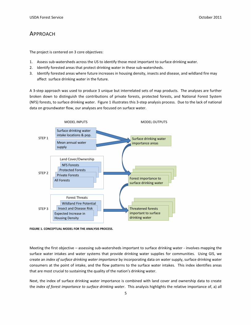
A 3-step approach was used to produce 3 unique but interrelated sets of map products. The analyses are further

broken down to distinguish the contributions of private forests, protected forests, and National Forest System

(NFS) forests, to surface drinking water. Figure 1 illustrates this 3-step analysis process. Due to the lack of national

data on groundwater flow, our analyses are focused on surface water.

STEP 3

Forest Threats

Surface drinking water importance areas

Threatened forests important to surface drinking water

Surface drinking water intake locations & pop.

Mean annual water supply

MODEL INPUTS MODEL OUTPUTS

STEP 1

STEP 2

Wildland Fire Potential

Insect and Disease Risk

Expected Increase in Housing Density

Land Cover/Ownership

NFS Forests

Protected Forests

Private Forests

All Forests Forest importance to surface drinking water

FIGURE 1. CONCEPTUAL MODEL FOR THE ANALYSIS PROCESS.

Meeting the first objective – assessing sub-watersheds important to surface drinking water - involves mapping the

surface water intakes and water systems that provide drinking water supplies for communities. Using GIS, we

create an index of surface drinking water importance by incorporating data on water supply, surface drinking water

consumers at the point of intake, and the flow patterns to the surface water intakes. This index identifies areas

that are most crucial to sustaining the quality of the nation’s drinking water.

Next, the index of surface drinking water importance is combined with land cover and ownership data to create

the index of forest importance to surface drinking water. This analysis highlights the relative importance of, a) all


6

forest lands, b) National Forest System lands, c) unprotected private forest lands, and d) protected (public and

private) forest lands. The results of this step are used to identify sub-watersheds where each category of forest

lands is most important in protecting surface drinking water.

We then look beyond the forests’ role in providing critical watershed services, to understand where the contribution of forests to surface drinking water might be affected by three threats—fire, insects and disease, and development. We focus on these threats because we were able to acquire high quality national spatial datasets, relevant at the spatial scale of this analysis. Data for each of these threats is combined with the results from the second objective. Watersheds are then ranked for each threat, with the highest values being in areas that are highly threatened,, highly forested, and highly important for surface drinking water quality.

ArcGIS 9.3 (ESRI, 2009) with the Spatial Analyst extension was used to conduct all spatial analyses, while R Statistical Software (R Development Core Team, 2006) was used for flow modeling and computations.


7

SCALE

The 12-digit Hydrologic Unit Code (HUC) was used as the unit of analysis. There are over 90,000 of these

delineated sub-watersheds in the US, and their average size is roughly 35 square miles. Analysis at this scale

provides information useful for States, counties, and National Forests while affording the opportunity for

summarization of findings at larger watershed scales and standardized comparison across the country. The 12-

digit HUC scale is also most appropriate for evaluating risk factors since the spatial importance of these risks are

often lost when summarized at larger scales. Despite being at the 12-digit HUC scale, the final map results are not

intended to assess individual HUCs of interest, but rather to be used to gain a broad understanding of the trends

and patterns across the landscape. We encourage further site-specific and localized analyses incorporating

additional local data when interested in the impacts and options for management in particular local areas. This is

particularly encouraged for addressing additional forest threats—such as road construction—that this analysis has

not considered. See Using the Data section for additional discussion.

The dataset of 12-digit HUCs (NRCS/USDA, 2009) provided the vector delineation of the 12-digit HUCs along with

identification of the downstream HUC which form the basis of the flow modeling. Any missing, non-existent, or

other erroneous downstream HUC attributes were manually corrected by referring to the hydrography network

and flow data from the NHDPlus dataset (EPA, 2006).


8

STEP ONE: IMPORTANT AREAS FOR SURFACE DRINKING WATER

Overview

A variety of approaches have been taken to model important drinking water protection areas. These often take

the form of a zone drawn around each surface drinking water intake based on a fixed or variable distance away

from the intake (i.e. EPA Source Water Area polygons), based on in-stream time of travel estimates, or based on

summarized water use data within watersheds. These efforts may be useful for local planning and immediate risk

mitigation, but often fail to consider the importance of terrestrial areas further upstream to the drinking water.

In an effort to account for the flow from land areas where supply originates to land areas where water is extracted

for use, and in order to consider the critical role of upstream areas in drinking water supply, we consider both the

land’s contribution to water supply (volume), the landscape surface flow patterns and the natural processes that

affect water quality, as well as downstream drinking water demand (consumption). Our model accounts for these

processes—water supply, spatial flow through the landscape, and the downstream drinking water demand.

Resulting maps display the relative importance of sub-watersheds for surface drinking water.

In its most basic form, the index of importance to surface drinking water (IMP) model can be broken down into

two parts:

IMPn = (PRn) * (Qn), (1)

where IMPn is the index of importance to surface drinking water for sub-watershed n, PRn is the risk-based drinking

water protection model for each sub-watershed n, and Qn is the mean annual water supply for each sub-watershed

n.

The risk-based drinking water protection model, PR, models the magnitude of demand and the flow patterns of

water to sites of withdrawal for use, while the mean annual water supply, Qn, represents the supply of water and

weights a sub-watershed based on how much water supply is generated on that land. When combined, the index

of importance to surface drinking water (IMP) includes areas important for providing water (water supply), areas

where drinking water is removed for use (water demand), and lands that connect the water supply and demand.

Drinking Water Protection Model, PR

Sediments and contaminants in water pose major difficulties for drinking water suppliers (Fowler, 2003). Pollution

from the land can force the need for new and costly technology to remove the contaminants, or it can place stress

and added costs on existing systems. If intake water quality is reduced, water treatment plants are faced with

increased levels of treatment and disinfection that can reduce the quality of water ultimately provided to the

public and even result in chemical by-products in drinking water, some of which may present new risks to public

health. As land changes from forest to other uses, additional risks of contamination increase. In extreme cases,

water services can be temporarily shut down when such conditions pose a risk to public health and in turn can

affect other water-dependent services. Unsurprisingly, keeping the level of sediment and contaminants low at the

drinking water intakes is a priority.


9

The drinking water protection index, PR, focuses on water demand and flow of water to the intakes and therefore

shows which areas have the highest potential to impact water quality through the input of sediments and

contaminants from the land. The model not only accounts for the importance of areas directly surrounding intakes

but also the upstream areas that contribute water to the point of withdrawal. The model incorporates the relative

consumer demand for surface drinking water by using the number of people served by each intake as a weighting

factor.

Locations and number of people served by each intake were provided by the US EPA Safe Drinking Water

Information System, SDWIS (EPA, 2009). In these analyses only the surface water springs, surface water intakes,

surface water reservoirs, and surface water infiltration galleries were used. Wells were included only where the

SDWIS database specified that groundwater was directly influenced by surface water. In general, groundwater

wells were not included. Consecutive connections, treatment plants, sampling stations, and non-piped drinking

water were not included in the analyses. Despite the variety of surface drinking water facilities included, in this

paper we refer to them collectively as “surface drinking water intakes” or simply “intakes.” The population served

at each intake was derived by dividing the number of people served in a drinking water system by the number of

intakes in the system. It is also important to note that intake locations in the SDWIS dataset are sited at the point

of water extraction, not at point of use.

As contaminants move through streams and rivers, they are affected by many processes including dilution,

dispersion, decay, and deposition. Many different types of sediment and nutrient transfer models have been used

to explain these processes (Reckow et al, 1989; Mulholland et al, 2009; Norris and Web, 1989). In this analysis, we

aim to represent these processes in a generalized way for multiple drinking water contaminants including

sediment. For every sub-watershed on the map, the drinking water protection model value equals the number of

people served by intakes in that sub-watershed plus a fraction of the population served by downstream intakes. In

this way it considers that risk to an intake declines with distance, and that peak concentrations decline moving

downstream.

The model component representing critically important areas close to intakes and upstream areas from where the

water flows is represented by this drinking water protection model (PR) is,

PRn = ∑ (Wi * Pi), (2)

where PRn is the drinking water protection model for each sub-watershed n, Pi is the population served by intakes

in the ith downstream sub-watershed from sub-watershed n, and Wi is the proportional weight for ith downstream

sub-watershed from sub-watershed n. Figure 2 provides an illustration of what this looks like across the US, and

Figure 3 shows a schematic for this equation.

Using literature review and consultation with our science advisory team, we defined the decreasing proportional

weights with distance upstream of an intake. We used an exponential decay relationship to represent the

relationship of distance from intake and relative importance to the surface drinking water. The proportional

weights, Wi, for the ith sub-watershed away from an intake in watershed n are based on the equation,

W = (1 - 0.01) ^ (d), (3)

where , W is the proportional weight and d is the distance from the intake and where each sub-watershed is

assumed to be 25km in stream length distance to the next sub-watershed. Figure 4 shows this equation


10

graphically, while Table 2 shows the proportional weights Wi, for the ith sub-watershed away from an intake in

watershed n.

At 70 km (43 mi) away from an intake, a sub-watershed counts 50% of the population served by the intake; at 225

km (140 mi), the sub-watershed counts only 10% of the population served by the intake.

FIGURE 2. DRINKING WATER PROTECTION MODEL, PR. FOR PURPOSES OF THIS MAP’S ILLUSTRATION, DATA WAS SPLIT INTO TEN GROUPS

WITH 10 REPRESENTING THE MOST IMPORTANT 10% OF AREAS.


11

FIGURE 3. SCHEMATIC OF DRINKING WATER PROTECTION MODEL, PR. THE DRINKING WATER PROTECTION MODEL VALUE EQUALS THE

NUMBER OF PEOPLE SERVED BY INTAKES IN THAT SUB-WATERSHED PLUS A FRACTION OF THE POPULATION SERVED BY DOWNSTREAM

INTAKES. IN THIS SCHEMATIC THERE ARE TWO INTAKES (STARS) THAT SERVE 10,000 PEOPLE EACH.

FIGURE 4. EXPONTIAL DECAY RELATIONSHIP BETWEEN DISTANCE FROM INTAKE, D, AND THE PROPORTIONAL WEIGHT, W.

0 100 200 300 400

0.0

0.2

0.4

0.6

0.8

1.0

Distance from intake (km), d

Pro

po

rtio

na

l W

eig

ht, W


12

TABLE 1. PROPORTIONAL WEIGHTS (FOR I=0 TO I=10) ROUNDED TO THE NEAREST THOUSANTH FOR EACH NTH UPSTREAM SUB-WATERSHED

IN EQUATION 2.

ith upstream HUC

Distance (km) upstream, d

Proportion Weight, W

0 0 1.000

1 25 0.779

2 50 0.607

3 75 0.472

4 100 0.368

5 125 0.287

6 150 0.223

7 175 0.174

8 200 0.135

9 225 0.105

10 250 0.082

Working at smaller spatial scales would allow for use of more extensive data on stream width, depth, and flow

patterns and amounts along many points of the water system. At the national scale a generalized decay

relationship was found to be a suitable method for providing a reasonable scale of the relative importance to the

surface drinking water.

Written out using the weights in Table 1, the drinking water protection model is,

PRn = 1.00*P0 + 0.78*P1 + 0.61*P2 + 0.47*P3 + 0.37*P4 + 0.29*P5

+ 0.22*P6 + 0.17*P7 + 0.14*P8 + 0.1*P9 + … + Wi * Pi (4)

A Special Case: The Great Lakes Region

Consistent methods were used across the United States with the exception of the Great Lakes region. The Great

Lakes are unique in that there are a large number of drinking water intakes found off-shore. To maintain a similar

weighting scenario, off-shore intakes were assigned to the closest sub-watershed and used together with all the

on-land intakes in the nation-wide drinking water protection model. Since intakes were located off-shore, all

areas bordering the Great Lakes affect the water quality of the off-shore intakes, not just the nearest sub-

watersheds where they were assigned. To account for the importance of all areas bordering the Great Lakes to the

water quality of the off-shore intakes, all sub-watersheds bordering the Lakes were identified (Figure 3a) and

assigned a small population value. Next, the drinking water protection model (Equation 2) was conducted for

those sub-watersheds alone (Figure 3b). Then the PR from the Great Lakes alone (Figure 3b) was added to the PR

for the nation (Figure 3c) to create the final PR value (Figure 3d). Although it is difficult to accurately assess the

relationships of adjacent lands and watersheds on specific off-shore intakes without substantial local information

about lake circulation and dynamics, we believe that this method provides a fair representation of the importance

of lands surrounding the Great Lakes to drinking water protection.


13

a)

b)

c)

d) FIGURE 5. THE GREAT LAKES REGION WAS HANDLED DIFFERENTLY TO ACCOUNT FOR THE IMPORTANCE OF ALL AREAS BORDERING THE

GREAT LAKES TO THE WATER QUALITY OF THE IN-LAKE INTAKES. SUB-WATERSHEDS BORDERING THE LAKES WERE IDENTIFIED (A) AND

ASSIGNED A SMALL POPULATION VALUE. NEXT, THE PR EQUATION (EQUATION 2) WAS RUN FOR THOSE SUB-WATERSHEDS ALONE (B).

THEN THE PR INDEX FROM THE GREAT LAKES ALONE (B) WAS ADDED TO THE PR INDEX FOR THE NATION (C) TO CREATE THE FINAL PR

VALUES (D).


14

Mean Annual Water Supply, Q

Many different methods have been used in the past to measure the relative water supply across the landscape.

The Forests, Water, People report (Barnes et al, 2009) on which this project was initially modeled, used an expert-

informed approach that combined indicators such as percent intact riparian buffer, road density, and percent

forest to predict the ability of a land to produce clean water. This type of approach is better suited to regional or

local scale analyses that share the same general ecological trends and relationships. Because of the national focus

of this assessment, and recognition of the heterogeneity of water yield across the US, Brown, et al’s (2008) water

balance based modeling of mean annual water supply for our measure of relative water supply (Figure 5) was used

to create a weighting of geography for water supply. Brown estimates water supply across the United States as

precipitation minus evapotranspiration across the period 1953 to 1994. Details on this methodology can be found

in Brown, et al (2008).

By including water supply in the model as a weight, areas that provide very little water are weighted lower on the

final IMP index. In Eastern US where mean annual water supply is fairly evenly distributed, the affect of applying

this weighting makes very little difference on the final model results. In the West, where mean annual water

supply is far more variable and heavily dependent on elevation, the final IMP values are affected more

substantially. For example, the dry Central Valley of CA is down-weighted, while the weighting of upstream

forested Sierra headwaters that generate much more of the total water yield are increased.

FIGURE 6. MEAN ANNUAL WATER SUPPLY, Q, IN MM/YR FROM PERIOD 1953-1994 FROM BROWN, ET AL (2008).


15

The Final Model: Index of Importance to Surface Drinking Water, IMP

The final model of surface drinking water importance combines the drinking water protection model (PRn),

capturing the flow of water and water demand, with Brown et al’s (2008) model of mean annual water supply (Qn).

The values generated by the drinking water protection model are simply multiplied by the results of the model of

mean annual water supply to create the final surface drinking water importance index. Expressed fully, the surface

drinking water importance index is,

impn = (Qn) * (∑ (Wi * Pi)). (5)

The final non-zero outputs were split into 100 quantiles, or 100 groups with approximately 1% of the data each.

This ranks the relative importance from least, 0, to most, 100.

The final map of the Surface Drinking Water Importance Index (see Figure 7) shows areas that are important to

surface drinking water supplies across the US. The high values across much of the eastern US are due to high

population density relative to other parts of the country and a greater reliance on surface water than on

groundwater. The lower values shown for much of the arid West are due to lower population density and a much

greater reliance on groundwater systems. It is important to note that this model does not explicitly consider water

scarcity. As a result, much of the arid West, though facing challenging drinking water supply issues, does not have

high IMP values. In addition, states like Wisconsin and Florida, and many southeastern coastal areas that have

high reliance on groundwater sources of drinking water also have lower IMP values.

FIGURE 7. SURFACE DRINKING WATER IMPORTANCE INDEX, IMP.


16

STEP TWO: FOREST IMPORTANCE TO SURFACE DRINKING WATER

The surface drinking water importance index (IMP) described in the previous section, shows the relative

importance of geographic areas across the country (watersheds) for surface drinking water, but does not

distinguish between land cover types. To determine the extent to which forests in particular are currently

protecting these areas we created an index of forest importance to surface drinking water by weighting the surface

drinking water importance index, IMP, by the percent of forest in each sub-watershed. This is represented by:

FIMPn = (IMPn) * (FORn) / 100, (6)

where FIMPn is the index of forest importance to surface drinking water, IMPn is the surface drinking water

importance index, and FORn is the percent forest land in each sub-watershed n. Both IMP and FOR range from 0 to

100, and so the final FIMP values will also fall between 0 and 100. In this way areas with small amounts of forests

will have a small FIMP value no matter what IMP value the sub-watershed had. Similarly, areas with small IMP

values will have small FIMP values no matter what FOR value it had. Only areas with high IMP and FOR values will

also have high FIMP values.

The data used to distinguish between non-forest, protected forest, private forest, and forest land managed by the

USDA Forest Service, was derived from the National Land Cover Dataset (USGS, 2007), data on National Forest

System land locations (USFS, 2009), and the Protected Areas Database (CBI, 2006). Classes 41, 412, 43, and 9 from

the National Land Cover Dataset were considered forest. All remaining areas were labeled as non-forest. The

Index of forest importance to surface drinking water is repeated for each forest type so that:

PriFIMPn = (IMPn) * (PriFORn), (7)

ProFIMPn = (IMPn) * (ProFORn), (8)

nfsFIMPn = (IMPn) * (nfsFORn), (9)

where PriFIMP, ProFIMP, and nfsFIMP are indices of forest importance to surface drinking water for private forest,

protected forest, and NFS lands, respectively; IMPn is the surface drinking water importance index; and PriFORn,

ProFORn, and nfsFORn are the percent private forest, protected forest, and NFS land, respectively, in each sub-

watershed n. Figure 8 shows the percent of each forest land (FORn, PriFORn, ProFORn, and nfsFORn) in each sub-

watershed n, and Figures 9-12 show the index of forest importance to surface drinking water for each forest land

(FIMP, PriFIMP, ProFIMP, and nfsFIMP). These maps identify those sub-watersheds where forest lands are most

important in protecting surface drinking water.


17

a)

b)

c)

d) FIGURE 8. PERCENT OF EACH SUB-WATERSHED THAT IS: A) ANY FOREST LAND, FOR; B) PRIVATE FORESTS, PRIFOR; C) PROTECTED FOREST,

PROFOR; AND, D) NFS FOREST LAND, NFSFOR.


18

FIGURE 9. THE INDEX OF FOREST IMPORTANCE TO SURFACE DRINKING WATER, FIMPN, IDENTIFIES THOSE SUB-WATERSHEDS WHERE FOREST

LANDS ARE MOST IMPORTANT IN PROTECTING SURFACE DRINKING WATER.

FIGURE 10. THE INDEX OF PRIVATE FOREST IMPORTANCE TO SURFACE DRINKING WATER, PRIFIMPN, IDENTIFIES THOSE SUB-WATERSHEDS

WHERE PRIVATE FOREST LANDS ARE MOST IMPORTANT IN PROTECTING SURFACE DRINKING WATER.


19

FIGURE 11. THE INDEX OF PROTECTED FOREST IMPORTANCE TO SURFACE DRINKING WATER, PROFIMPN, IDENTIFIES THOSE SUB-

WATERSHEDS WHERE PROTECTED FOREST LANDS ARE MOST IMPORTANT IN PROTECTING SURFACE DRINKING WATER.

FIGURE 12. THE INDEX OF NFS FOREST IMPORTANCE TO SURFACE DRINKING WATER, NFSFIMPN, IDENTIFIES THOSE SUB-WATERSHEDS

WHERE NFS FOREST LANDS ARE MOST IMPORTANT IN PROTECTING SURFACE DRINKING WATER.


20

STEP THREE: THREATS TO FORESTS IMPORTANT FOR SURFACE DRINKING WATER

Overview

Intact and healthy functioning forests are of critical importance to the provision of high quality drinking water.

Wildfire, increased insect and disease, and land development can all have impacts on sediment and contaminant

levels in waterways. Though fire is a natural occurrence in many forests, in extreme cases wildfires can increase

sediment loads significantly with serious downstream consequences for water supplies. Treatment works and

reservoirs as far as 100 miles downstream from a fire can be affected by increased sediment loads, as was the case

with the Fall 2003 wildfires in the Santa Ana Watershed of Southern California (Meixner and Wohlgumuth, 2004).

Apart from sediment, wildfire can lead to increases in nitrogen (Landsburg and Tiedemann, 2000), phosphorus

(Landsburg and Tiedemann, 2000), mercury, dissolved salts (Van Lear and Waldrop, 1989), and retardant residues

from fire suppression efforts (Norris and Webb, 1989).

Although insects and diseases are part of natural ecosystems, invasive insects and disease, in addition to climate

change, and forest overcrowding have created areas with widespread die-off of forests with impacts on drinking

water. In extreme cases, insects and diseases can fundamentally altered forest structure and function. This in turn

can result in increased erosion and affect nutrient cycling among other ecosystem services. In addition, these

forested areas weakened by insects and diseases are at higher risk of experiencing high intensity fires that could

further affect downstream water quality.

Water quality impacts from wildfire, insects and diseases often produce short-term declines in water quality.

However, the addition of housing and related infrastructure to the landscape results in permanent conversion of

the forest to other uses and is thus more likely to produce long term, chronic, water quality problems.

Development affects water quality through initial land disturbance and erosion (including road-building), increases

the risk for introduction of chemicals and other contaminants, and increases impervious surface which speeds

transfer of contaminants from terrestrial areas to rivers as well as leading to stream instability. Development’s

effects of water supply are of critical importance to address.

In this third and final step of the analysis, we identify forested areas important for surface drinking water that are

likely to be affected by future increases in housing density, insects and diseases, and wildland fire. The procedures

utilized for this step were tiered from similar analyses undertaken by the Forests on the Edge project (Stein et al

2009). Such analyses have been used to identify areas where private forest benefits could be most impacted by

each of these threats, and can be useful in identifying areas where surface drinking water supply could be most

threatened.

Although there are many forest threats that can affect drinking water quality, our analysis includes only those

described here. Other threats were not included because they were not relevant at the spatial scale of this analysis

or because we did not find reliable, nationally-available spatial data. Despite our focus on development, insects

and disease, and fire, it is possible to use the results from step one and two along with other threats data perhaps

available at for a smaller area (region, state, etc.). See the Using the Data section for additional discussion.


21

To begin, we multiply the index of forest importance to surface drinking water, the output from step two, by a

value 0-100 that represents the percent of a watershed that is highly threatened by a given threat. This is

expressed as,

(FIMPn) *(THRn) / 100, (10)

or in full expression,

(IMPn) * (FORn) * (THRn) / 10000, (11)

where THRn is the percent of watershed n that is highly threatened by a given threat. In this paper, THR is defined

three times, once each for threat of development (dTHR), insects and disease (iTHR), and wildland fire (wTHR)

using externally created models of these threats and expert-recommended thresholds for what can be considered

“highly threatened.”

Increased Housing Density

To measure the threat of development we focused on increases in housing density. Housing density reflects a

change in the landscape more accurately than does population density alone. Projections of future housing

density increases on rural forest lands were used to quantify the threat of development across US forests.

The analysis used data layers produced by Stein et al (2009), who collapsed twelve categories of housing density

produced by Dave Theobald’s SERGoM v3 housing density model (Theobald, 2005) for 2000 and 2030, into 3

categories. We then subtracted the 2000 values from values expected for 2030 to create a GIS layer showing

expected increase in housing development between the years 2000 and 2030.

The three categories (Stein et al, 2009) were based on a review of the literature on impacts of development on

benefits provided by forests. The categories are: Rural 1 (> 40 acres per housing unit), Rural 2 (10-40 acres per

housing unit), or Exurban Rural (less than 10 acres per housing unit). Any change from Rural 1 to Rural 2, Rural 2 to

Exurban/Urban, or Rural 1 to Exurban/Urban were considered as areas “highly threatened” by development.

Roughly 26% of the continental US, and 15% of forest lands falls in this highly threatened category (Figure 13).

When summarized by sub-watershed, an average of 17% of the forested lands were highly threatened by

development.

The percent of forested land highly threatened by development in each sub-watershed, dTHR, was used as the THR

input into this third step. The final expression used for development threat is,

(FIMPn) *(dTHRn) / 100. (12)

Figure 14 shows these values visually. On a scale from 0 to 100, the mean is 3.23 and the standard deviation is 7.7.


22

FIGURE 13. PERCENT OF EACH SUB-WATERSHED EXPECTED TO EXPERIENCE AN INCREASE IN HOUSING DENSITY IN FORESTED AREAS

BETWEEN 2000 AND 2030 (BASED ON STEIN ET AL, 2009 AND THEOBALD, 2005).

FIGURE 14. SUB-WATERSHEDS RANKED BY IMPORTANCE OF FORESTS FOR DRINKING WATER IMPORTANCE AND FUTURE HOUSING DENSITY

INCREASES COMBINED.


23

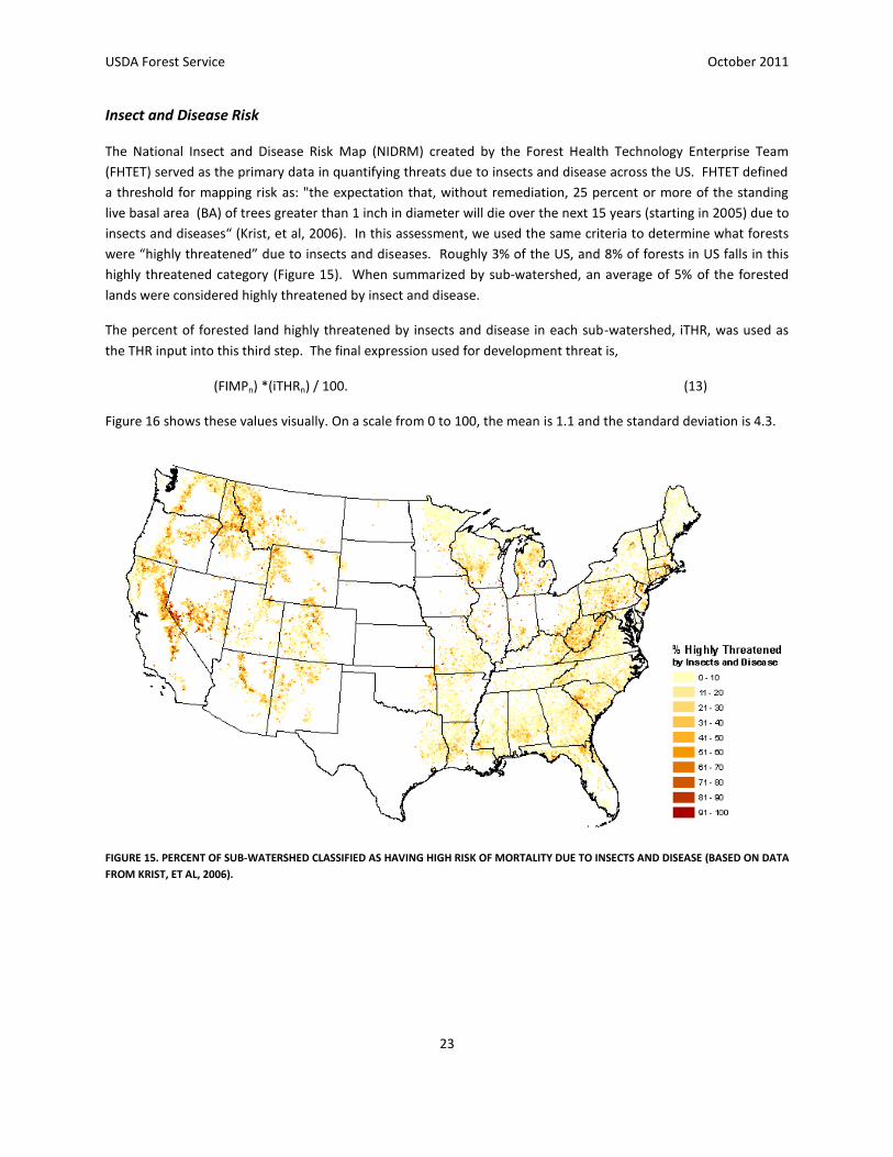
Insect and Disease Risk

The National Insect and Disease Risk Map (NIDRM) created by the Forest Health Technology Enterprise Team

(FHTET) served as the primary data in quantifying threats due to insects and disease across the US. FHTET defined

a threshold for mapping risk as: "the expectation that, without remediation, 25 percent or more of the standing

live basal area (BA) of trees greater than 1 inch in diameter will die over the next 15 years (starting in 2005) due to

insects and diseases“ (Krist, et al, 2006). In this assessment, we used the same criteria to determine what forests

were “highly threatened” due to insects and diseases. Roughly 3% of the US, and 8% of forests in US falls in this

highly threatened category (Figure 15). When summarized by sub-watershed, an average of 5% of the forested

lands were considered highly threatened by insect and disease.

The percent of forested land highly threatened by insects and disease in each sub-watershed, iTHR, was used as

the THR input into this third step. The final expression used for development threat is,

(FIMPn) *(iTHRn) / 100. (13)


FIGURE 15. PERCENT OF SUB-WATERSHED CLASSIFIED AS HAVING HIGH RISK OF MORTALITY DUE TO INSECTS AND DISEASE (BASED ON DATA

FROM KRIST, ET AL, 2006).


24

FIGURE 16. SUB-WATERSHEDS RANKED BY IMPORTANCE OF FORESTED AREAS FOR SURFACE DRINKING WATER AND BY PECENTAGE

CLASSIFIED AS HAVING HIGH RISK OF MORTALITY DUE TO INSECTS AND DISEASE.

Wildfire Risk

To assess forests’ risk for wildfire, we used the Wildland Fire Potential data created by the USFS National Fire

Institute. Wildland Fire Potential delineates areas based on fire intensity, weather, fire frequency, and size, which

are then classified into a relative ranking of fire potential ranging from very low to very high. Potential fire severity

is based on surface fuels potential and crown fire potential. Surface fuel potential is based on calculated values for

rate of spread and flame lengths, using the National Fuel Characterization Classification Systems. Crown fire

potential was based on assigned relative classes of fire intensity for a current vegetation cover type. Fire weather

potential is based on the average number of days per year the relative energy release component was above the

95 percentile from 1980 to 2005, and the average number of days a year that experienced extreme fire weather

based on thresholds of temperature, wind, and humidity from 1982 to 1997. Fire frequency and size is based on

the number of 1/10 acre fires or greater per million acres and the number of 500 acres fire or greater per million

acres from 1986 to 1996. (USDA Forest Service, Fire Modeling Institute, 2008)

For this analysis, areas were included that ranked as having high or very high wildland fire potential. Roughly 26%

of the continental US, and 35% of all forest falls into one of these categories. When summarized by sub-

watershed, an average of 29% of the forested lands in each watershed are identified as having high or very high

wildland fire potential. (Figure 17).

Fire affects watershed stability and water quality differently depending on many factors including geographic

region, distance of fire to water source, local topography, soil type, slope, and weather patterns. In addition,


25

forest fire is a natural process and is critically important to the natural functioning of many forests. When

interpreting the output map (figure 18), it is important to consider this.

The percent of forested land in each sub-watershed identified as having high or very high wildland fire, fTHR, was

used as the THR input into this third step. The final expression used for development threat is,

(FIMPn) *(fTHRn) / 100. (14)


FIGURE 17. PERCENT OF SUB-WATERSHED CONTAINING FORESTS WITH HIGH OR VERY HIGH WILDLAND FIRE POTENTIAL (BASED ON DATA

FROM USFS FIRE MODELING INSTITUTE).


26

FIGURE 18. SUB-WATERSHEDS RANKED ACCORDING TO IMPORTANCE OF FORESTED AREAS FOR DRINKING WATER AND PERCENTAGE OF

FOREST IDENTIFIED AS HAVING HIGH WILDLAND FIRE POTENTIAL COMBINED.


27

APPLICATIONS

Introduction

The results of this assessment provide critical information that can identify areas of interest for protecting surface

drinking water. The spatial dataset can be incorporated into broad-scale planning, such as the State Forest Action

Plans, and can help identify areas for further local analysis. In addition it can be incorporated into existing decision

support tools that currently lack spatial data on important areas for surface drinking water. This project also sets

the groundwork for identifying watersheds where a payment for watershed services (PWS) project may be an

option for financing conservation and management on forest lands. This work can serve as an education tool to

illustrate the link between forests and the provision of surface drinking water – a key watershed-based ecosystem

service.

All maps in this Forests to Faucets analysis are intended to show general trends across broad areas at the sub-

watershed scale. They are valuable tools for decisions regarding prioritization of actions across the landscape.

Due to the geographic scope of this project, we employed models general enough to work at the national scale.

Any specific forest management decisions should be based on local considerations. Because of this, we

recommend further spatial analysis conducted a finer scale to better incorporate localized data, and consideration

of local on-the-ground understanding of the environmental processes.

Potential Sites for Payment for Watershed Services

Payments for Watershed Services (PWS) describes a variety of mechanisms by which providers of watershed

services are financially compensated by beneficiaries of these services. A common form of PWS is an upstream-

downstream transaction where downstream users such as water utilities pay upstream landowners to employ

management practices that improve or maintain watershed services. Financing of watershed management

through Payments for Watershed Services not only connects the forests to the faucet in economic terms, but also

incentivizes watershed protection which leads to net increases in forest protection and improved management.

Although there are many criteria for successful PWS projects, the Forests to Faucets project ranks areas based on

three baseline criteria: (1) a connection between forest management and clean water, (2) a consumer demand for

the clean water, and (3) a threat to the existing watershed services that can be avoided or averted through a

payment designated for management or protection. On a macro scale, the Forests to Faucets assessment identifies

these areas— areas with a great ability to supply clean water, a large consumer demand for this water, and facing

significant forest threats.

Spatial Decision Support Tools

In most areas, surface drinking water quality is one of many considerations that guide conservation and

management decisions. Others include threatened and endangered species habitat, cost of implementing a project

and level of political support for conserving or managing a certain area. Spatial decision support tools can help to

weigh these considerations. Despite the important role spatial decision support tools can play in defining


28

management priorities, acquiring high quality spatial data can be a challenge. Without a comprehensive national

dataset showing importance of upstream areas for surface drinking water quality, existing spatial decision support

models have not been able to adequately consider the importance of upstream areas for surface drinking water

quality. The Forests to Faucets national dataset, will enable the surface drinking water quality to be included in

new and existing spatial decision support tools. Examples of such decision-support tools include the Hazardous

Fuels Priority Allocation System from the US Forest Service Fire Program. Other prioritization decision-support

models and processes where Forests to Faucets data may be employed include the State Forest Action Plans and

the US Forest Service Watershed Condition Framework prioritization.


29

ACKNOWLEDGEMENTS This work would not have been possible without the groundwork of the “Forests, Water, and People” project by

Martina Barnes, Al Todd, Rebecca Lilja, and Paul Barten. Work by the Forests on the Edge project was also

important in guiding the threats analyses that we performed. Our science advisory team of Tom Brown (USFS

Rocky Mountain Research Station), Jim Vose (USFS Coweeta Hydrologic Laboratory), Steve McNulty (USFS

Southern Research Station) and Paul Barten (University of Massachusetts) provided critical advice throughout the

project. Frank Krist, Frank Sapio, Jim Menekis, Susan Stein, Karl Dalla Rosa, Jean Thomas, Chris Carlson, Rick

Swanson, and many others provided support as project advisors. Nicole Balloffet, Steve Marshall, Paul Ries, and

the entire Ecosystem Services Program Area staff were invaluable resources throughout all phases of the Forests to

Faucets project development.

CORRESPONDENCE We encourage you to be in touch with any questions and comments about the methods and potential uses of the

data. Please address correspondence to Emily Weidner, [email protected].

mailto:[email protected]


30

REFERENCES Barnes, M., A. Todd, R. Lilja, and P. Barten. 2009. Forests, Water and People: Drinking water supply and forest

lands in the Northeast and Midwest United States. USDA Forest Service, Northeastern Area State and

Private Forestry. NA-FR-01-08. June 2009.

Brown, T., M. Hobbins, and J. Ramirez. 2008. Spatial distribution of water supply in the coterminous United

States. Journal of the American water Resources Association. 44(6):1474-1487.

Conservation Biology Institute (CBI). Protected Areas Database, Version 4. [CD-ROM] Corvallis, OR: 2006.

ESRI (Environmental Systems Resource Institute). 2009. ArcGIS 9.3. ESRI, Redlands, California.

Fowler, C. 2003. Human health impacts of forest fires in the Southern US: A literature review. Journal of Ecological

Anthropology. 3:39-63.

Krist, F., F. Sapio, B. Tkacz. 2006. Mapping Risk from Forest Insects and Diseases. Forest Health Technology

Enterprise Team, USDA Forest Service. FHTET 2007-06.

Landsburg, J. and A. Tiedemann. 2000. “Fire Management,” in Drinking water from forests and grasslands: A

synthesis of the scientific literature. Edited by G. Dessmeyer, pp. 124-138. GTR-SRS-39. Ashville, NC:

USDA Forest Service, Southern Research Station.

Meixner, T. and P. Wohlgemuth. 2004. Wildfire Impacts on Water Quality. Southwest Hydrology. Sep/Oct 2004.

URL http://www.swhydro.arizona.edu/archive/V3_N5/feature7.pdf

Mulholland, P., H.M. Valett, J. Webster, S. Thomas, L. Cooper, S. Hamilton, B. Peterson. 2009. Nitrate removal in

stream ecosystems measured by 15N addition experiments: Denitrification. Limnol. Oceanogr. 54(3):666-

680.

Norris, L., and W. Webb. 1989. Effects of fire retardant on water quality. USDA Forest Service General Technical

Report, PSW-109. 1989. URL:

http://www.fs.fed.us/psw/publications/documents/psw_gtr109/psw_gtr109_79.pdf

R Development Core Team (2006). R: A language and environment for statistical computing. R Foundation for

Statistical Computing, Vienna, Austria. ISBN 3-900051-07-0, URL http://www.R-project.org.

Stein, S. R. McRoberts, L. Mahal, M. Carr, R. Alig, S. Comas, D. Theobald, and A. Cundiff. 2009. Private Forests,

Public Benefits: Increased Housing Density and Other Pressures on Private Forest Contributions. USDA

Forest Service, Pacific Northwest Research Station, PNW-GTR-795. December 2009.

Theobald, D. 2005. Landscape patterns of exurban growth in the USA from 1980 to 2020. Ecology and Society.

10(1):32.

USDA/NRCS, National Cartography & Geospatial Center. 12-Digit Watershed Boundary Data 1:24,000 [dataset].

Fort Worth, TX. (Data Access from FS NRIS 02-03-2009)

USDA Forest Service, Corporate Data Warehouse. ALP NFS Basic Ownership [dataset]. May, 2009.

http://www.r-project.org/


31

USDA Forest Service, Forest Health Technology Enterprise Team (FHTET). National Insect & Disease Risk Map.

[dataset], USDA Forest Service, Pacific Northwest Research Station. Portland, OR, 2007. Available online

at: http://www.fs.fed.us/foresthealth/technology/nidrm.shtml.

U. S. Environmental Protection Agency (EPA). Safe Drinking Water Information System (SDWIS) [dataset].

Washington, DC: U.S. EPA. June, 2009.

U.S. Environmental Protection Agency (EPA). National Hydrography Dataset Plus (NHDPlus) [dataset].

Washington, DC: U.S. EPA. 2006.

U.S. Geological Survey (USGS). 2001 National land cover data set. [dataset]. Sioux Falls, SD: 2007.

Van Lear, D. and T. Waldrop. 1989. History, uses, and effects of fire in the Appalachians. GTR-SE-54. Asheville, NC:

USDA Forest Service, Southeastern Forest Experiment Station.


32

APPENDIX 1: DATA README FILE The “Forests to Faucets” data includes two files, one representing the data inputs, “F2F_inputs.dbf,” and one

representing the data outputs, “F2F_outputs.dbf.” In each file the unique row identifier is the 12-digit HUC code,

“HUC1.” To view the data spatially, download the 12-digit HUC vector data from USGS, and join the DBF tables

using the HUC code as the unique identifier. Please refer to the “From the Forest to the Faucet: Drinking Water

and Forests in the US” methods paper for detailed methods and data citations.

The list below describes the attributes of the “F2F_inputs.dbf” file:

HUC1: The 12-digit HUC code that uniquely identifies each HUC

HUC2: The 12-digit HUC code that uniquely identifies each downstream HUC

PopServed: Number of people served by intakes found in the HUC. Actual values have been deleted. All

values are 0 in the data provided. Contact EPA Headquarters to get access to the data.

Q_model: Mean Annual Water Supply, Q, from period 1953-1994 from Brown, et al (2008).

2PER_FOR: Percent forest in HUC

2PER_PRONF: Percent protected forest (including NFS forest) in HUC

2PER_NFS: Percent NFS forest in HUC

2PER_PRI: Percent private forest in HUC

3PER_INSEC: Percent of HUC highly threatened by Insects and Disease (using FHTET National Insect and

Disease Risk Map)

3PER_DEV: Percent of HUC highly threatened by development (using Dave Theobald’s data for predicted

housing density increase)

3PER_FIRE: Percent of HUC highly threatened by wildland fire (using National Fire Laboratory data for

wildland fire risk)

The list below describes the attributes of the “F2F_outputs.dbf” file:

HUC1: The 12-digit HUC code that uniquely identifies each HUC

HUC2: The 12-digit HUC code that uniquely identifies each downstream HUC

1IMP: Index of importance to surface drinking water, IMP, ranked and normalized to be on a 0-100 scale.

2IN_FOR: Index of forest importance to surface drinking water, FIMP. Created by multiplying “1IMP” by

“2PER_FOR”

2IN_PRONF: Index of protected forest importance to surface drinking water, PronfFIMP. Created by

multiplying “1IMP” by “2PER_PRONF”

2IN_NFS: Index of NFS forest importance to surface drinking water, nfsFIMP. Created by multiplying

“1IMP” by “2PER_NFS”

2IN_PRI: Index of private forest importance to surface drinking water, PriFIMP. Created by multiplying

“1IMP” by “2PER_PRI”

3_INS_FOR: Index of insect and disease threat to forests important to surface drinking water. Created by

multiplying “2IN_FOR” by “3PER_INSEC”

3_DEV_FOR: Index of development threat to forests important to surface drinking water. Created by

multiplying “2IN_FOR” by “3PER_DEV”

3_FIR_FOR: Index of wildland fire threat to forests important to surface drinking water. Created by

multiplying “2IN_FOR” by “3PER_FIRE”


33

APPENDIX 2: EPA SAFE DRINKING WATER INFORMATION SYSTEM (SDWIS)

What is the SDWIS dataset?

EPA’s Safe Drinking Water Information System (SDWIS) databases store information about drinking water.

The federal version (SDWIS/FED) stores the information EPA needs to monitor approximately 156,000

public water systems. Information in the dataset includes:

Basic information on each water system, including: name, ID number, city county, and number of

people served, type of system (residential, transient, non-transient), whether they operate year-

round or seasonal, and characteristics of their sources of water

Violation information for each water system: whether it has followed established monitoring and

reporting schedules, complied with mandated treatment techniques, violated any Maximum

Contaminant Levels (MCLs), or communicated vital information to their customers

Enforcement information: what actions states have taken to ensure that drinking water systems

return to compliance if they are in violation of a drinking water regulation

Sampling results for unregulated contaminants and for regulated contaminants when the

monitoring results exceed the MCL

Spatial data is available in latitude/longitude format or as small source water protection areas in

vector data.

How do I get access to the dataset?

You may access statistical information on local drinking water from SDWIS/FED in the following ways:

1. Browse and/or download Annual Public Water System Statistics PDF

The following summary tables include inventory data on water systems, violations reported by

violation type and by contaminant/rule, and official Government Performance and Results Act

(GPRA) data.

http://water.epa.gov/scitech/datait/databases/drink/sdwisfed/howtoaccessdata.cfm

2. Access data on individual water systems online through Envirofacts. These include basic inventory

data, violations reported, and enforcement actions taken against individual water systems in the

past 10 years. http://www.epa.gov/enviro/html/sdwis/sdwis_ov.html

3. Download and manipulate SDWIS/FED data in MS Excel PivotTables®

Access aggregated information on all violations reported in an EPA region, state, and county since

1993 using the MS Excel PivotTables®. These multidimensional tables contain aggregated

information on water systems; violations reported by violation type and by contaminant/rule, and

GPRA data, for each year since 1993; and current Envirofacts data. Sort, categorize, and analyze

the data across several dimensions.

http://water.epa.gov/scitech/datait/databases/drink/pivottables.cfm

4. Read the annual Consumer Confidence Report (also called a water quality report) published by

your public water system. Each year by July 1st you should receive in the mail an annual water

quality report (consumer confidence report) from your water supplier that tells where your water

comes from and what's in it. http://cfpub.epa.gov/safewater/ccr/index.cfm

http://water.epa.gov/scitech/datait/databases/drink/sdwisfed/howtoaccessdata.cfm

http://www.epa.gov/enviro/html/sdwis/sdwis_ov.html

http://water.epa.gov/scitech/datait/databases/drink/pivottables.cfm

http://cfpub.epa.gov/safewater/ccr/index.cfm


34

5. Make a Freedom of Information Act (FOIA) Request. Visit the EPA Freedom of Information Office

Web site for instructions. http://www.epa.gov/foia/

The SDWIS dataset with its latitude/longitude is not classified, but is considered sensitive information, and

thus requires signing a confidentiality agreement. (And therefore researchers involved in the Forests to

Faucets project may not distribute this information to any internal or external partners.) Make the

following EPA contact to request access to the GIS data for the nation or to ask more detailed questions

about the SDWIS dataset.

Towana Dorsey SDWIS Security Awareness Lead

[email protected] 202-564-4099

Who do I contact with questions about SDWIS dataset?

Check this website for User Support and Training related to the SDWIS dataset, and contact information for

the SDWIS hotline, national and regional representatives.

http://water.epa.gov/scitech/datait/databases/drink/sdwisfed/datamanagers_usersupport.cfm

http://www.epa.gov/foia/

mailto:[email protected]

http://water.epa.gov/scitech/datait/databases/drink/sdwisfed/datamanagers_usersupport.cfm

from the forest to the faucet - home | us forest service

Documents