from supply to demand factors: what are the determinants

HAL Id: hal-02883545https://hal-enpc.archives-ouvertes.fr/hal-02883545

Submitted on 29 Jun 2020

HAL is a multi-disciplinary open accessarchive for the deposit and dissemination of sci-entific research documents, whether they are pub-lished or not. The documents may come fromteaching and research institutions in France orabroad, or from public or private research centers.

L’archive ouverte pluridisciplinaire HAL, estdestinée au dépôt et à la diffusion de documentsscientifiques de niveau recherche, publiés ou non,émanant des établissements d’enseignement et derecherche français ou étrangers, des laboratoirespublics ou privés.

From supply to demand factors: what are thedeterminants of attractiveness for outdoor recreation?

Léa Tardieu, Laetitia Tufféry

To cite this version:Léa Tardieu, Laetitia Tufféry. From supply to demand factors: what are the determinants ofattractiveness for outdoor recreation?. Ecological Economics, Elsevier, 2019, 161, pp.163 - 175.�10.1016/j.ecolecon.2019.03.022�. �hal-02883545�

https://hal-enpc.archives-ouvertes.fr/hal-02883545

https://hal.archives-ouvertes.fr

Post-Print version available at https://authors.elsevier.com/a/1YqKW3Hb~0IYY1

1

From supply to demand factors: what are the determinants of attractiveness for

outdoor recreation?

Léa Tardieu1* and Laetitia Tuffery2 Ecological Economics 161, 163-175 – July 2019

Abstract

The concept of ecosystem services (ES) remains underused in supporting practical decisions in conservation/development plans and programs. One of the most important factors explaining this non-consideration is the lack of spatial information describing the nature-society relationship in environmental and economic analyses. In this paper, we developed a novel method to predict, in spatially explicit terms, the recreation attractiveness potential combining supply and demand factors. Our method is based on the combination and transfer of a Lancasterian function of biophysical aspects and a travel cost model based on agents’ sociodemographic characteristics. We further validate the usefulness of the proposed recreation model by using it in the evaluation of a regional park charter pursuing two main objectives: recreational attractiveness and habitat quality (modeled with InVEST). The results demonstrate first that the biophysical context plays a large role in the recreational trip choice and thus should not be ignored in travel cost studies. Second, from a policy guidance perspective, we show that providing spatial information appears particularly critical for ES to be a useful lever for action in day-to-day decision-making.

Keywords: Forest recreational attractiveness, Supply and demand factors, Travel cost method, Function benefit transfer, Regional park strategy.

JEL codes: Q26, Q51, R12, R58

1 CIRED, AgroParisTech, Cirad, CNRS, EHESS, Ecole des Ponts ParisTech, Université Paris-Saclay, F-94736, Nogent-sur-Marne, France. Email: [email protected] *Corresponding author.

2 BETA, Université Lorraine, INRA, AgroParisTech, F-54000, Nancy, France. Email: [email protected]


2

1. INTRODUCTION

Despite the growing political attention paid to social dependencies of human beings on natural systems, these dependencies remain under-considered in practical decisions with regard to conservation and management plans (Laurans et al., 2013). One of the most important factors explaining this non-consideration is the lack of spatial information describing the nature-society relationship in environmental and economic analyses. Ecosystem services (ES) modeling and mapping is now recognized as a unifying approach for different research communities to support the consideration of this link for decision-making (Bateman et al. 2014, Burkhard and Maes, 2017). Refined techniques for mapping the supply side (representing ES flows produced by the ecological functioning of ecosystems), the demand side (flows to beneficiaries) or different values associated with ES have been developed. By providing spatially explicit representations of ES, land managers have the opportunity to broaden the goals that can be pursued when evaluating land management scenarios (Geneletti, 2016). For instance, winners and losers of potential land management decisions affecting ES can be more clearly identified and located by using these types of analysis.

Nevertheless, shortcomings remain in this field because of a lack of combined consideration of both ecological and social aspects of ES. This leads spatial models to be based predominantly on biophysical attributes, ignoring individuals’ preferences for these attributes, or to a lesser extent, based on socioeconomic drivers while ignoring ecological flows of ES (Tardieu, 2017). A good example for the latter case is the recreational service for which, in contrast to other ES in the literature, the modeling of the demand side is much more developed than that of the supply side (Termansen et al., 2013).

Since Hotelling’s letter in 1947, recreation demand has been historically assessed by modeling visits with the travel cost method. The method enables a recreation demand function to be derived for predicting a participation decision and the number of trips taken to a site according to an implicit price (the travel cost) and a set of other variables (time available, income, other available sites as substitutes, visitors’ socioeconomic characteristics, etc.) (e.g., Shresta et al., 2002; Parsons, 2003; Martínez-Espiñeira and Amoako-Tuffour, 2008; Bujosa Bestard and Riera Font, 2010; Jones et al., 2010; Binner et al., 2017). The advantage of the method is that it relies on real individuals’ behaviors (revealed preference) and allows the assessment of the actual benefits derived from existing policies or management types (from an ex-post perspective). However, the produced results are often (1) aggregated numbers of visits that do not allow a spatial differentiation of recreation trips within the destination site and (2) focused on individuals, while underestimating the importance of the biophysical characteristics of destination sites.

Other approaches enable the recreational service to be modeled and mapped. Colson et al. (2010) relied on a survey in which forest managers reported the visitation frequency to forests in Wallonia, enabling the attributes explaining forest attractiveness to be determined.

Other new methods based on volunteered geographic information such as self-geotagged photographs on web applications directly uploaded by visitors (e.g., Flickr©) may allow the development of spatially sensitive recreation maps. Finally, Zulian et al. (2014) developed the ESTIMAP model to map the recreation potential across Europe. However, these models do not rely on individuals’ recreation preferences. Instead, recreation potential often assumes


3

implicitly that visitors' preferences are the same regardless of the sociodemographic characteristics of potential users, with the main driver of recreation being the distance/accessibility, and, more importantly, that every individual (located at the right distance from the recreational site) is a potential user. According to the wide literature in economics on this subject, this assumption is far from being verified. Moreover, no demand evolution, consequent to a change in sociodemographic context, can be predicted from these models.

Termansen et al. (2013), Johnston et al. (2015) and Czajkowski et al. (2017) mapped recreational values by transferring a function derived from a discrete choice experiment (DCE) study applied from national surveys. De Valck et al. (2017) also mapped site quality scores from a distance-based DCE. However, although these studies consider visitors’ characteristics and preferences, they do not characterize the actual demand in terms of visits, provided that the DCE is based on hypothetical situations of policy initiatives or management alternatives (from an ex-ante perspective). In one exception, Sen et al. (2014)3 took into account the spatial variability of recreational services, based on actual visits, and combine supply and demand factors in their study. The authors developed a model to predict visits, obtained from a national recreation survey, according to destination site characteristics, the attributes of outset locations and the distance traveled by visitors to reach the site. They further applied the estimated model to the national scale in the United Kingdom. Nevertheless, whether these types of models are applicable to more local territories, requiring more precise output data to develop accurate strategies at the local scale remains an open question.

In this paper, we rely on existing and observed data to derive recreation functions, according to supply and demand factors, in spatially explicit terms at the local level to inform decision-making. We develop a methodology to predict, in a spatially sensitive way, the recreation supply and demand of forest ecosystems. The developed method can be applied to any other ecosystem type. The predictions are based on a Lancasterian function of biophysical supply and a travel cost method to inform visitation preferences. We further upscale the supply and demand functions to the studied area. In this way, this study constitutes one of the first attempts to develop a function benefit transfer based on a travel cost method enabling transferring a recreation function adjusted for on-site attributes and individual preferences. We apply the method to a real case study of a regional park in France to test its applicability. Then, we validate the usefulness of the created output by using it to evaluate the regional park charter. Because the park charter is developed around two objectives, biodiversity conservation and recreational attractiveness, we add a habitat quality index in the evaluation, which is computed with the InVEST4 model.

We show that site attractiveness is driven both by the biophysical attributes of forests and the socioeconomic characteristics of individuals, the former having a stronger effect. This finding calls for a better accounting of these attributes in travel cost methods that tend to ignore key

3 The paper by Sen et al. (2014) is mostly based on various seminal papers developing the use of GIS in travel cost techniques: Jones et al. (2010), Brainard et al. (1997 and 1999) and Lovett et al. (1997). 4 Integrated valuation of ecosystem services and trade-offs from the Natural Capital Project. InVEST is an open-source software available at: https://www.naturalcapitalproject.org/invest/ (webpage access date 02/14/19)


4

factors of recreational attractiveness or to better account for individual preferences in studies focusing on supply factors. Second, we show that the created indexes, expressed as geographic information, can provide policy guidance for territorial management planning by allowing overlapping layers to inform multiple objectives (i.e., biodiversity conservation and region attractiveness).

2. MATERIALS AND METHODS

2.1. Snapshot of the methodological framework

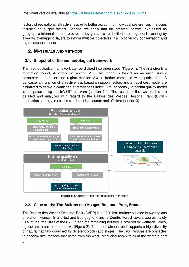
The methodological framework can be divided into three steps (Figure 1). The first step is a recreation model, described in section 2.3. This model is based on an initial survey conducted in the Lorraine region (section 2.3.1), further combined with spatial data. A Lancasterian function of attractiveness based on supply factors and a travel cost model are estimated to derive a combined attractiveness index. Simultaneously, a habitat quality model is computed using the InVEST software (section 2.4). The results of the two models are detailed and analyzed with regard to the Ballons des Vosges Regional Park (BVRP) orientation strategy to assess whether it is accurate and efficient (section 3).

Figure 1: Snapshot of the methodological framework

2.2. Case study: The Ballons des Vosges Regional Park, France

The Ballons des Vosges Regional Park (BVRP) is a 2700 km2 territory situated in two regions of eastern France: Grand-Est and Bourgogne Franche-Comté. Forest covers approximately 61% of the total area of the BVRP, and the remaining territory is covered by wetlands, lakes, agricultural areas and meadows (Figure 2). The mountainous relief supports a high diversity of natural habitats governed by different bioclimatic stages. The High Vosges are obstacles to oceanic disturbances that come from the west, producing heavy rains in the western part


5

of the BVRP (more than 2 m/year) to the crest line and, conversely, approximately 50 cm/year in the eastern part, making this side of the park one of the driest regions in France. One-third of BVRP territory has been placed under "remarkable natural site" status and 22% under Natura 2000 conservation commitments5. A few remarkable species are present in the site, such as Western capercaillie (Tetrao urogallus) and the lynx (Lynx lynx), which are subject to particular conservation programs. In terms of recreation, the BVRP is a popular site for skiing and hiking activities.

Natural Regional Park is a protection status in France6. Such parks are governed by a charter approved by the states and municipalities composing the area. The charter sets the development strategy in terms of the maintenance/improvement of environmental and cultural heritage and the means to implement it over a 15-year period. According to the charter, the environmental strategy must be focused on two principal activities: (1) recreational attractiveness and (2) habitat and biodiversity conservation. To that end, land managers have developed a management strategy, specified in the 2024 horizon charter, for three different territories (Figure 2). First, in the High Vosges territory, the objective is to ensure habitat conservation while maintaining good recreational attractiveness. More specifically, managers rely on the European Charter for Sustainable Tourism in Protected Areas7 and try to define tourist attendance strategies. Second, the key challenge in the Valleys and Piedmont is to control urbanization and habitat fragmentation. Finally, the 1000

Ponds Plateau benefits from exceptional habitat richness; however, declines resulting from industrial and farmland activities are weakening the attractiveness of this area. Thus, the objective in this area is to sustain its vitality.

5 More information on the park charter is available online (webpage access 02/11/14): https://issuu.com/parcdesballons/docs/charte_2012-2024_fevrier2014 6 French environmental code (Article L333-1) modified after the Law on Biodiversity 2016 (L2016-1087 8 août 2016, Article 48). 7http://www.europarc.org/library/europarc-events-and-programmes/european-charter-for-sustainable-tourism/ (webpage access date 01/25/19)


6

Figure 2: The land cover types (a) and the three main territories of the Ballons des Vosges Regional Park (b)

2.3. Recreation model

2.3.1. Original survey and scales of analysis

We rely on an online survey initially conducted in the former Lorraine region (now the Grand-Est region), covering one-third of the BVRP territory (Figure 3). This survey has been used in different cases to study local recreation by Abildtrup et al. (2015a and 2015b). The survey

(a)

(b)


7

was carried out between July and August 2010 by email in the former Lorraine region. A total of 1144 respondents completed the survey, and 526 had visited a forest and provided information about which specific forest they had visited in the 12 months before the survey (i.e., July/August 2009 – July/August 2010). All of the survey details are reported in Abildtrup et al. (2015a and 2015b).

In the initial survey, Lorraine’s forests were divided into “forest units" representing relevant recreational units equal to or greater than 5 ha. A total of 5568 forest units were delineated in the initial survey. From this total sample, we selected the forest units included in the BVRP, which are in the Vosges department in the Lorraine region, resulting in 256 forest units. In total, 1236 visits were recorded in 94 of the 256 forest units and distributed throughout the entire area of the BVRP, surrounded by a 10 km buffer zone8 (Figure 3). Our recreation model is developed based on those 94 forest units. However, because we had no clear rules to define forest units in the rest of the BVRP area, we defined recreational units through a raster distributed homogeneously according to a kilometric mesh (1*1 km). Based on the French forest database (BD Forêt®, IGN), we assigned the surface of forest areas to each mesh. Only meshes including at least 50% of the closed canopy forest were considered as forest recreational units in this work. Meshes cover the entire area of the park, expanded through a 10 km buffer zone around its perimeter to take into account possible visitors who live just outside the park and, therefore, to avoid border effects. Ultimately, we obtained 3774 forest recreational units over the entire BVRP (Figure 3). These recreational units were used to upscale recreational functions.

Figure 3: Area covered by the initial survey in the BVRP, the forest units visited, and the kilometric mesh used for

the benefit transfer

8 We considered this buffer zone because forest units are sometimes juxtaposed with BVRP territory or are very close to the limits of the BVRP.


8

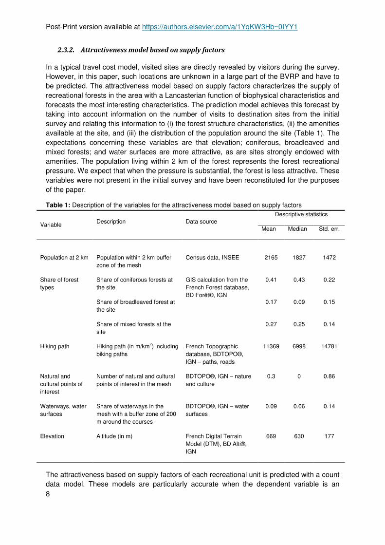
2.3.2. Attractiveness model based on supply factors

In a typical travel cost model, visited sites are directly revealed by visitors during the survey. However, in this paper, such locations are unknown in a large part of the BVRP and have to be predicted. The attractiveness model based on supply factors characterizes the supply of recreational forests in the area with a Lancasterian function of biophysical characteristics and forecasts the most interesting characteristics. The prediction model achieves this forecast by taking into account information on the number of visits to destination sites from the initial survey and relating this information to (i) the forest structure characteristics, (ii) the amenities available at the site, and (iii) the distribution of the population around the site (Table 1). The expectations concerning these variables are that elevation; coniferous, broadleaved and mixed forests; and water surfaces are more attractive, as are sites strongly endowed with amenities. The population living within 2 km of the forest represents the forest recreational pressure. We expect that when the pressure is substantial, the forest is less attractive. These variables were not present in the initial survey and have been reconstituted for the purposes of the paper.

Table 1: Description of the variables for the attractiveness model based on supply factors

Variable Description Data source Descriptive statistics

Mean Median Std. err.

Population at 2 km

Population within 2 km buffer zone of the mesh

Census data, INSEE

2165

1827

1472

Share of forest types

Share of coniferous forests at the site

GIS calculation from the French Forest database, BD Forêt®, IGN

0.41 0.43 0.22

Share of broadleaved forest at the site

0.17 0.09 0.15

Share of mixed forests at the site

0.27 0.25 0.14

Hiking path Hiking path (in m/km2) including biking paths

French Topographic database, BDTOPO®, IGN – paths, roads

11369 6998 14781

Natural and cultural points of interest

Number of natural and cultural points of interest in the mesh

BDTOPO®, IGN – nature and culture

0.3 0 0.86

Waterways, water surfaces

Share of waterways in the mesh with a buffer zone of 200 m around the courses

BDTOPO®, IGN – water surfaces

0.09 0.06 0.14

Elevation Altitude (in m) French Digital Terrain Model (DTM), BD Alti®, IGN

669 630 177

The attractiveness based on supply factors of each recreational unit is predicted with a count data model. These models are particularly accurate when the dependent variable is an


9

integer that takes few values, such as visitors’ trips to a destination site (Shaw, 1988; Englin and Shonkwiler, 1995; Baerenklau et al., 2010, Roussel et al., 2016).

Many pixels are not visited. We addressed this issue by using a zero-inflated count data model, where the probability of participation is estimated simultaneously with the visit function (Cameron and Trivedi, 1986; Gurmu and Trivedi, 1996). Zero-inflated count data models are more general than typical count models in that they relax the restriction that an identical process generates both zeros and positive integers. Moreover, as Englin et al. (2003) argue and as it is the case in our dataset, zero trips can be generated by both a binomial process (for people not in the market, i.e., not visiting any forests) and a Poisson process (for people in the market, i.e., surveyed visitors who did not take any trips in the specific forest in question).

In contrast to simple-hurdle models, zero-inflated models account for both types of zeros by following a two-step procedure. First, a participation model determines whether the zero observation belongs to the group where the dependent variable is always null (i.e.,

nonvisitors) or whether it belongs to the group in which the dependent variable can be positive or null (i.e., visitors). Furthermore, a Poisson or a negative binomial regression estimates the visit function. Thus, the density function with a Poisson distribution for each forest � is as follows (Englin and Shonkwiler, 1995):

�� = �|� = �� + �1 − ��e�� = 0�1 − � �e�λ� �� ! �� > 0 �1�

where �� is the probability that a visitor coming from an outset location � will take no trip to

forest � and �1 − �� is the probability that �� follows a Poisson law with a λ� parameter (see

Roussel et al. (2016) for more explanations on the standard Poisson model).

For the λ parameter representing the average number of visits, � is dependent on a vector of explanatory variables that can be different from , the vector of the explanatory variables for λ . Participation can be either assessed with a logit or a probit model, depending on the distribution we assume.

2.3.3. Attractiveness model based on demand factors

Attractiveness based on demand is derived from the initial survey by applying a travel cost model. This model aims to predict the trips taken to each forest recreational unit from any given outset area. To allow the trip function to be transferable, we limited the number of variables to those that can be reconstituted on non-surveyed individuals (e.g., income, distance from the outset location to forest). Moreover, as Bateman et al. (2011) suggest, this type of parameterization excluding ad hoc variables is recommended because of the multiplicative role of coefficients resulting in major transfer errors in over-parameterized models. We thus derive a recreation demand function from the travel cost model determined by an implicit price (the trip cost) and a set of independent variables (generic predictors of individual demand based on economic theory such as the availability of substitutes and income).


10

The trip cost is a combined cost between trip costs for individuals using motorized means of travel and an opportunity cost of time. The trip cost is computed as follows:

"# = 2 × &�'��( × #�)�� + *#"+ �2� where "# is the trip cost and '��( is the distance between the outset location and the site9 in km. #�) is a cost per km based on the vehicle fiscal power published annually by the fiscal administration. Because we did not have this information, we made the assumption that vehicles had a mean fiscal power of 4 fiscal horsepower (the highest proportion of registered vehicles in France since 2000 have between 4 and 5 fiscal horsepower10), corresponding to a cost of 0.493/km11. This cost takes into account vehicle depreciation, maintenance costs, tire expenses, fuel consumption and insurance premiums. � is the number of individuals in the group. The costs are multiplied by two to consider the entire round trip. We did not consider foot and bicycle travel, even though some studies considered material depreciation in terms of cycle or trekking shoes (e.g., Bertram et al., 2017). *#" is the opportunity cost of time. An individual who visits a recreation site has an opportunity to use his time differently (working, for example) and is therefore subject to an opportunity cost. This cost relies on the assumption of an individual’s trade-off between labor and leisure. However, we chose not to consider an *#" for two reasons: (i) because we rely on very local recreation, implying short trips to forests, and (ii) because this approach assumes that individuals have flexible jobs and are able to substitute work for leisure time at the margin, and this assumption is rarely verified12.

As in the attractiveness model based on supply factors, visits are predicted with a count data model where the dependent variable is the number of observed visits in each forest unit �. The observations come from the initial survey. The dependent variables are recomputed to serve our trip function transfer and are described in Table 2. The expectations regarding these variables are that the trip cost between the respondent’s outset location and the visited site lowers visit demand as well as the availability of substitutes around the outset location and that the income increases recreation demand.

9 D, the distance between the outset location and the forest, is calculated by using the osrmtime command from Stata (Huber and Rust, 2016). 10https://www.statistiques.developpement-durable.gouv.fr/donnees-sur-les-immatriculations-des-vehicules (webpage access date 12/03/18) 11 K takes into account vehicle depreciation, maintenance, fuel and insurance costs and is published annually by the fiscal administration in France (webpage access date 12/01/16) https://www3.impots.gouv.fr/simulateur/calcul_impot/2017/pdf/baremekm.pdf This inclusion of vehicle depreciation is typical in the TCM (see Parsons, 2003). However, this inclusion has been discussed in the literature (see Earnhart, 2003) because individuals may not explicitly perceive these types of costs. 12 For a discussion regarding the OCT, refer to Roussel et al. (2016).


11

Table 2: Variables used in the attractiveness model based on demand factors and in the transfer Variables Description Data source Descriptive statistics

Mean Median Std. err.

Visits Visits reported by visitors in the year preceding the survey

Survey 15.63 6 23.5

TC (Trip cost)

Initial survey

Calculated from the centroid of the visitors' IRIS13 to the recreational unit centroid

GIS calculation, ESRI ArcGIS

16.20 10.46 23.93

Reconstituted variable in the transfer

Calculated from each IRIS centroid to each recreational unit centroid with Equation 1

Income (€) Initial survey

Median individual net income in different income classes

Census data INSEE 33007 33750 14581


Median individual net income at the IRIS level

Availability of substitutes

Initial survey

Share of other land use types around a 5 km14 buffer around the visitor’s IRIS centroid

GIS calculation (ESRI ArcGIS) from Corine Land Cover (2012)

% Urban areas (CLC1) 0.38 0.25 0.34 % Agricultural areas (CLC2) 0.25 0.24 0.27

% Wetlands (CLC4) 0.001 0 0.008

% Water bodies (CLC5) 0.008 0 0.014

% Coniferous forests (CLC311) 0.19 0.14 0.18

% Broadleaved forests (CLC312) 0.05 0 0.15

% Mixed forests (CLC313) 0.04 0 0.11


Share of other land use types within a 5 km buffer around the IRIS centroid

2.3.4. Benefit transfer and construction of the combined attractiveness index

Two transfer functions are completed to map the combined attractiveness index (CAI) of BVRP forests:

13 IRIS (Ilots Regroupés pour l'Information Statistique) is the smallest level of French national statistics, and it includes approximately 2000 persons. 14 The 5 km buffer was chosen following Sen et al. (2014), who tested different radiuses (1 km, 2.5 km, 5 km, and 10 km). The 5 km radius had the best fit according to the Akaike Information Criterion (AIC).


12

(1) A transfer of the function developed in the attractiveness model based on supply factors that leads to the development of an attractiveness supply index (ASI); and

(2) A trip transfer function predicting the visits to BVRP territory, allowing the development of the attractiveness index based on demand factors (ADI).

In the case of the attractiveness model based on supply factors, the significant coefficients are applied to each 1 km2 mesh of recreational units in the park. The result, after normalization, gives the ASI based on the characteristics sought by visitors. The ASI for each cell � varies between [0; 1] and is calculated as follows:

/01 = /0 − /02 3/0245 − /02 3 �3� where /0 = exp�9�� , ∀� �4� /0 is the attractiveness score based on the supply of recreational cell �, with � ∈=1, … , 1? before normalization. �� is a vector of the supply independent variables (the same variables as those described in Table 1) describing recreational forest unit � in the entire park, and 9 is a vector of the estimated parameters associated with the vector �� in the attractiveness model based on supply factors (specified as a zero-inflated Poisson (ZIP) model, which is why the functional form of the equation is semi-logarithmic).

Furthermore, the demand function is applied to construct the ADI applied to the variables described in Table 2.

/'1 = /' − /'2 3/'245 − /'2 3

where �5�

/' � = exp�D"# � + EF�� , ∀�, ∀� and /' = J /' �

K�LM , ∀�, ∀� �6�

/' is the attractiveness based on demand factors of recreational cell � from a series of outset locations present in the BVRP, with � ∈ =1, … , 1? before normalization. As in the common travel cost, it also denotes the number of visits to cell �. /' � is the demand for cell � from a given visitor coming from an outset location �, with � ∈ =1, … , P?. F�� is the vector of

demand independent variables describing visitors and the outset area � characteristics, i.e., the percentage of various land use types within a set radius of the outset location. "# � is the

travel cost between recreational cell � and outset �. All the variables are described in Table 2. E and D are the vector of parameters associated with the trip cost and other variables estimated in the attractiveness model based on demand factors.

Finally, the CAI is attributed to each recreational unit � by computing the geometric mean of the two indexes as follows:


13

#/1 = Q/01 × /'1 �7� Using a geometric mean makes it possible to consider non-compensation between the two indexes. That is, the ASI and the ADI cannot completely compensate for each other in the CAI if the ASI is strong and the ADI is weak or vice versa. Therefore, a strong combined index reveals strong attractiveness of supply factors combined with a strong attractiveness of demand factors (which is symmetrical for a low CAI).

2.4. Habitat quality index

Several tools and models to spatially assess natural habitat quality are already available; they are usually based on ecological indicators (Maes et al., 2012) or on ecological modeling, such as Globio and Marxan (Alkemade et al., 2009; Chan et al., 2011), or on land use land cover change modeling, such as InVEST (Kareiva et al., 2011; Terrado et al., 2016; Sallustio et al., 2017; Salata et al., 2017). We use the InVEST model of habitat quality as a proxy to represent biodiversity richness. The aim is to estimate the quality of habitats in spatially explicit terms by measuring the appropriate conditions for the survival and reproduction of species generally based on the potential threat and degradation of natural habitats (Tallis et al., 2011).

Land cover is composed of seven categories extracted from the Corine Land Cover database (CLC, 2012): artificial areas (CLC1), agricultural lands (CLC2), coniferous forests (CLC311), broadleaved forests (CLC312), mixed forests (CLC313), semi-natural areas (CLC32), and water bodies (CLC4-CLC5). Thus, only forests are considered and more precisely identified (i.e., three categories of forestland cover), as our analysis is based on only the habitat quality of forest areas.

Habitat degradation and quality are functions of threats from different sources, e.g., artificial areas, agricultural lands, main roads, secondary roads, and trails. Artificial areas and agricultural lands are included as sources of landscape fragmentation and habitat degradation (Girvetz et al., 2008). In addition, a few studies have revealed the important impact of forest roads on biodiversity and forest habitat (e.g., Marcantonio et al., 2013). Consequently, analysis of road networks according to their categorization (primary, secondary and trails, derived from the French Topographic database, BDTOPO®) is critical to understanding the role of linear infrastructure on habitat loss, fragmentation, and degradation (Underhill and Angold, 2000; Von Der Lippe and Kowarik, 2008).

The habitat quality index depends on four factors: ST, the impact of the threats on habitat (i.e., relative impact of each threat to other threats on habitat quality, ranging from 0 to 1); UVW. ', the distance between habitat and threats (i.e., maximum distance, in km, under which each threat affects habitat quality)15; X�, the habitat suitability (classification, from 0 to 1, of land-covers as habitat); and 0�T, the sensitivity of habitats to threats (ranging from 0 to 1).

Based on these different factors, the degradation level ' � is defined as follows:

15 The distance decay is defined by the InVEST model as exponential (Tallis et al, 2011).


14

' � = J J Y ST∑ [\]\LM ^ T_a

_LM]

\LM W\_ ��\ �8� where c is a mesh of the threat raster T, dT represents all the meshes of the raster T, ST is the relative weight of the impact of threat T, W\_ is the impact of threat T that originates in grid

cell c on the habitat in grid cell � (function of the distance), and 0�\ is the sensitivity of

habitat � to threat T.

After computing the degradation level, the habitat quality e � is defined as follows:

e � = X� f1 − Y ' �' � + g^h �9� X� ranges from 0 to 1, where 1 indicates LULC classes with the highest suitability for species

and g is the half-saturation constant, i.e., 50% of the maximum level of degradation that our territory can support. The degradation (Equation 8) is then translated into habitat quality level according to the half-saturation constant (Equation 9), with UVW' � = 0.8; g = 0.4 in this

case study. Thus, the higher the degradation index ' � and the half-saturation constant g are, the lower the quality of habitats e � . To define the parameters of the model, we used a combined approach based on a literature review (Polasky et al., 2011; Terrado et al., 2016; Salata et al., 2017; Sallustio et al., 2017) and participatory meetings with local stakeholders and managers. More specifically, we first defined our scores based on their absolute and, more importantly, their relative values according to the literature. Then, our scores were further discussed and validated by our panel of experts (a public forest manager, a biodiversity officer in the BVRP, and a forest officer of the National Geographic Institute). These experts are specialists in biodiversity protection issues, ecological corridors (e.g., forest continuum, network of wetlands) and forest management. Inputs are presented in Tables 3 and 4.

Table 3: The characteristics of the threats to habitat quality in the BVRP Type of threat T

Maximum distance UVW. '

Impact weight ST

Artificial areas 1.5 0.9 Main roads 1.5 0.9 Secondary roads 1 0.7 Agricultural land 1 0.56 Trails 0.3 0.35

Table 4: Habitat suitability and the sensitivity to each threat in the BVRP

Forest cover Habitat suitability X� Urban

Agriculture

Road1 0�T

Road2

Trail

Broadleaved forest 0.9 0.8 0.5 0.8 0.6 0.4 Coniferous forest 0.8 0.72 0.45 0.72 0.54 0.36 Mixed forest 0.9 0.8 0.5 0.8 0.6 0.4


15

3. RESULTS AND DISCUSSION

3.1. Recreation model

3.1.1. Attractiveness model based on supply factors

We estimated four count data models: a Poisson model, a Zero Inflated Poisson (ZIP) model, a negative binomial model and a zero-inflated negative binomial model. The likelihood ratio test on alpha, representing the dispersion parameter, showed that our dataset was not overdispersed, justifying the use of a Poisson model over a negative binomial model. Vuong’s test confirmed that the ZIP model was preferable to a standard Poisson model (z>2) (Vuong, 1989).

We tested various model specifications, including the following: - Hiking paths as the number of paths instead of meters; - Waterways and forest surfaces instead of coverage share variables; - Public versus private forests; - Distance to the nearest forest; and - Different variables explaining non-visited forests.

We present the best fitting model according to the Akaike information criterion (AIC) and Bayesian information criterion (BIC) model selection criteria in Table 5.

Table 5: Zero-inflated Poisson model for the attractiveness model based on supply factors of destination sites

Variables ZIP coefficients Std. Err.

Trip demand Population 2 km around the site -4.87e-05 (3.18e-05) Log (% of broadleaved forests at the site) -0.100*** (0.0287) Log (% of mixed forest at the site) 0.0807** (0.0390) Natural and cultural points of interest at sites (number of points) 0.521*** (0.0457) Waterways, water surfaces (% of the surface) 0.996** (0.416) Elevation -0.00646*** (0.00138) Squared elevation 7.88e-06** (9.66e-07) Hiking path (in m/km²) -1.16e-05 (7.32e-06) Squared hiking path (in m/km²) 0 (1.29e-10) Constant 5.608*** (0.448) Participation Hiking path (in m/km²) -5.84e-05** (2.48e-05) Squared hiking path (in m/km²) 7.41e-10* (4.02e-10) Constant 0.917*** (0.237) Log likelihood -1038.1072 LR chi2 (9) 268.85377 Prob>chi2 0.000 AIC 2098.2144 BIC 2135.9372 Number of zero observations 162 Number of non-zero observations 94 Total observations 256 Standard errors in parentheses *** p<0.01, ** p<0.05, * p<0.1 Vuong’s test of ZIP vs. standard Poisson: z=5.76, Pr>z=0.0000


16

Alpha test on ZINB=1.948269, Pr>z=0.286 Coniferous forests are set as the reference of coverage share.

We can observe that the most powerful predictor is elevation, followed by the presence of water and the presence of natural and cultural points of interest at the site. This result is also observed in previous studies based on stated preferences (e.g., Nielsen et al., 2007; Colson et al., 2010; Abildtrup et al., 2013; Termansen et al., 2013, De Valck et al., 2014; Zulian et al., 2014 and De Valck, 2017). Forest types are integrated as logarithms and can thus be interpreted as elasticities. Mixed forests provide the greatest attraction compared to coniferous and broadleaved forests. These types of forest characteristics are, to the best of our knowledge, rarely integrated in models explaining recreational visits, making comparisons difficult. However, some studies have integrated some of these characteristics in their regressions. For instance, Sen et al. (2014) found a positive relationship between visits and the presence of woodland (they did not separate forest types). Termansen et al. (2013) and Colson et al. (2010) found a preference for broadleaved forest, and Schägner et al. (2016) found that the forest type had no effect.

The presence of a population at 2 km around the site has no impact on-site attractiveness. This finding invalidates the potential presence of a crowding effect in the area (Pröbstl et al., 2010), that is, a conflict between users and a congestion effect influencing attractiveness. The same result applies for the variable hiking path. This result contradicts our first intuitions and the findings in the literature (e.g., De Valck et al., 2017) but may be because the case study includes many hiking paths so that the variable does not discriminate between different supply units. Furthermore, elevation has a negative effect on attractiveness. Nevertheless, the square of elevation has a positive impact, giving an overall non-linear effect of elevation. That is, elevation decreases attractiveness to a certain point (823 m, in our case study), above which it increases attractiveness at higher elevations. This non-linearity is also observed in Colson et al. (2010) for the slope effect16. This result makes sense in a mountainous environment, such as the BVRP; indeed, it shows that individuals are more attracted by lowland and highland forests and have lower preferences for forests located in medium-altitude mountains.

The participation function is explained by only hiking path presence. Sites with fewer hiking paths are more likely to be visited, but the predictor is weak.

3.1.2. Attractiveness model based on demand factors

We estimated four count data models. However, for the same reasons, we ultimately relied on a ZIP model to explain attractiveness based on demand factors. The results are presented in Table 6. Other variables have been included to explain participation decision; however, none of them was significant.

16 Colson et al. (2010) modeled two slope variables as a proportion of woodland on slopes less than 10° and greater than 30°. They showed that woodlands located on slopes attract more visitors. However, overly steep slopes, that is, slopes greater than 30°, have the opposite effect, as is the case for many of our forests located below 823 m in our case study.


17

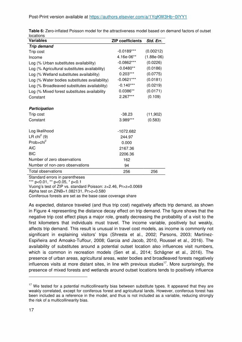
Table 6: Zero-inflated Poisson model for the attractiveness model based on demand factors of outset locations

Variables ZIP coefficients Std. Err.

Trip demand Trip cost -0.0189*** (0.00212)

Income 4.16e-06** (1.88e-06)

Log (% Urban substitutes availability) -0.0862*** (0.0226)

Log (% Agricultural substitutes availability) -0.0480** (0.0186)

Log (% Wetland substitutes availability) 0.203*** (0.0775)

Log (% Water bodies substitutes availability) -0.0621*** (0.0181)

Log (% Broadleaved substitutes availability) -0.140*** (0.0219)

Log (% Mixed forest substitutes availability 0.0386** (0.0171)

Constant 2.267*** (0.109)

Participation Trip cost -38.23 (11,902) Constant 3.989*** (0.583) Log likelihood -1072.682 LR chi2 (9) 244.97 Prob>chi2 0.000 AIC 2167.36 BIC 2206.36 Number of zero observations 162 Number of non-zero observations 94 Total observations 256 256 Standard errors in parentheses *** p<0.01, ** p<0.05, * p<0.1 Vuong’s test of ZIP vs. standard Poisson: z=2.46, Pr>z=0.0069 Alpha test on ZINB=1.082131, Pr>z=0.580 Coniferous forests are set as the base case coverage share

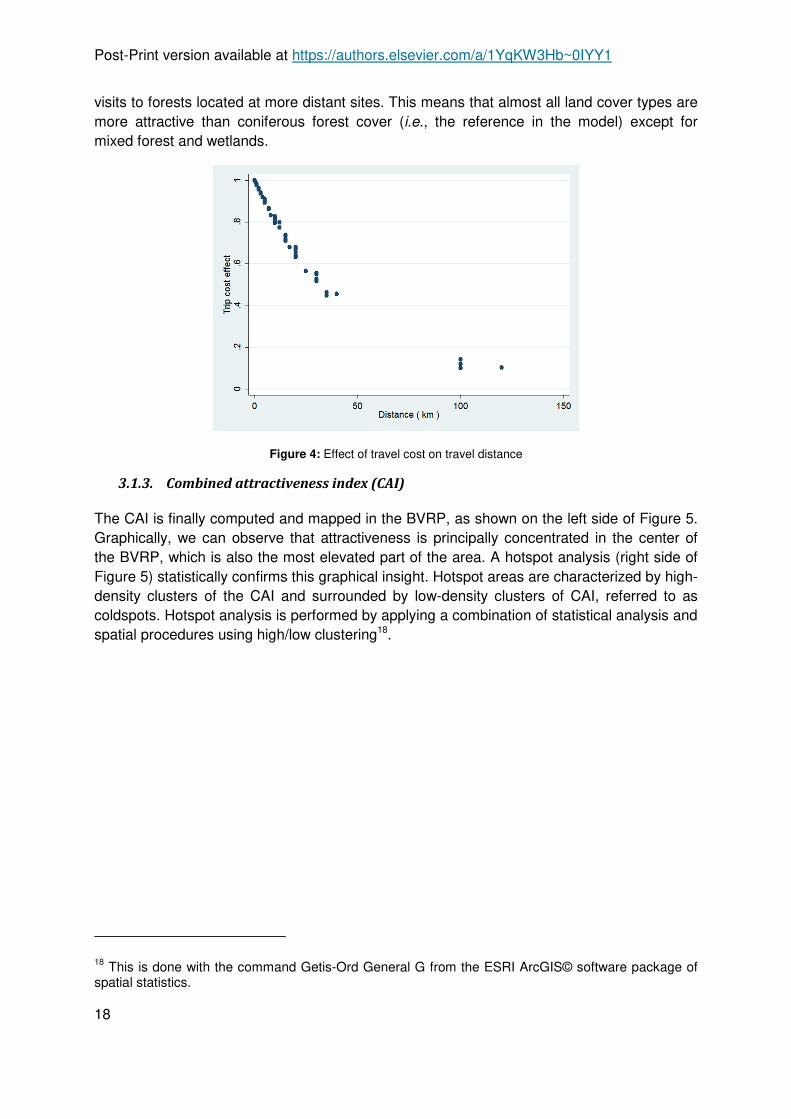
As expected, distance traveled (and thus trip cost) negatively affects trip demand, as shown in Figure 4 representing the distance decay effect on trip demand. The figure shows that the negative trip cost effect plays a major role, greatly decreasing the probability of a visit to the first kilometers that individuals must travel. The income variable, positively but weakly, affects trip demand. This result is unusual in travel cost models, as income is commonly not significant in explaining visitors’ trips (Shresta et al., 2002; Parsons, 2003; Martínez-Espiñeira and Amoako-Tuffour, 2008; Garcia and Jacob, 2010, Roussel et al., 2016). The availability of substitutes around a potential outset location also influences visit numbers, which is common in recreation models (Sen et al., 2014; Schägner et al., 2016). The presence of urban areas, agricultural areas, water bodies and broadleaved forests negatively influences visits at more distant sites, in line with previous studies17. More surprisingly, the presence of mixed forests and wetlands around outset locations tends to positively influence

17 We tested for a potential multicollinearity bias between substitute types. It appeared that they are weakly correlated, except for coniferous forest and agricultural lands. However, coniferous forest has been included as a reference in the model, and thus is not included as a variable, reducing strongly the risk of a multicollinearity bias.


18

visits to forests located at more distant sites. This means that almost all land cover types are more attractive than coniferous forest cover (i.e., the reference in the model) except for mixed forest and wetlands.

Figure 4: Effect of travel cost on travel distance

3.1.3. Combined attractiveness index (CAI)

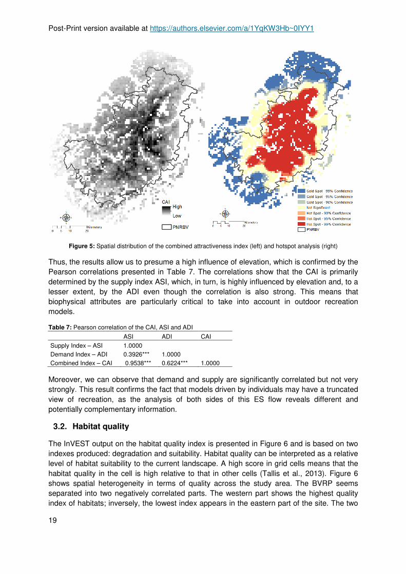
The CAI is finally computed and mapped in the BVRP, as shown on the left side of Figure 5. Graphically, we can observe that attractiveness is principally concentrated in the center of the BVRP, which is also the most elevated part of the area. A hotspot analysis (right side of Figure 5) statistically confirms this graphical insight. Hotspot areas are characterized by high-density clusters of the CAI and surrounded by low-density clusters of CAI, referred to as coldspots. Hotspot analysis is performed by applying a combination of statistical analysis and spatial procedures using high/low clustering18.

18 This is done with the command Getis-Ord General G from the ESRI ArcGIS© software package of spatial statistics.


19

Figure 5: Spatial distribution of the combined attractiveness index (left) and hotspot analysis (right)

Thus, the results allow us to presume a high influence of elevation, which is confirmed by the Pearson correlations presented in Table 7. The correlations show that the CAI is primarily determined by the supply index ASI, which, in turn, is highly influenced by elevation and, to a lesser extent, by the ADI even though the correlation is also strong. This means that biophysical attributes are particularly critical to take into account in outdoor recreation models.

Table 7: Pearson correlation of the CAI, ASI and ADI

ASI ADI CAI

Supply Index – ASI 1.0000 Demand Index – ADI 0.3926*** 1.0000 Combined Index – CAI 0.9538*** 0.6224*** 1.0000

Moreover, we can observe that demand and supply are significantly correlated but not very strongly. This result confirms the fact that models driven by individuals may have a truncated view of recreation, as the analysis of both sides of this ES flow reveals different and potentially complementary information.

3.2. Habitat quality

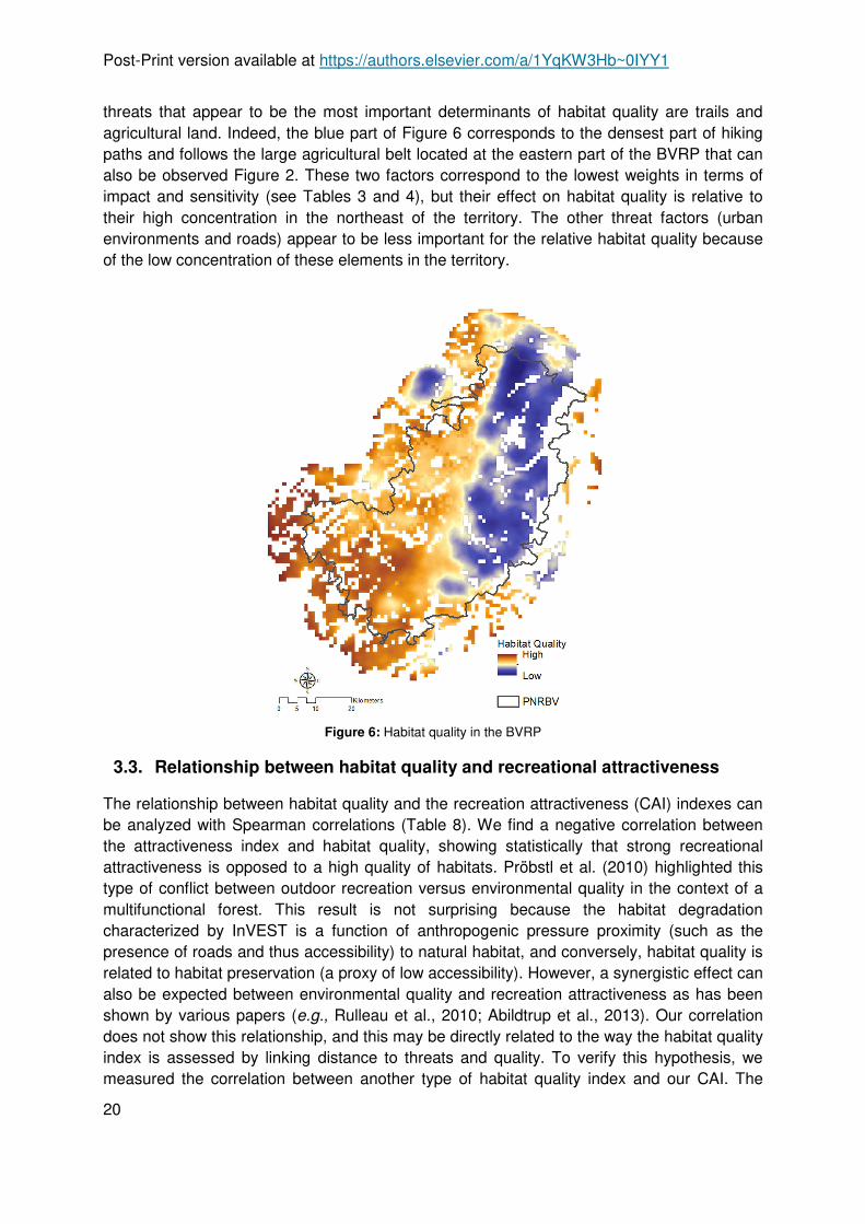
The InVEST output on the habitat quality index is presented in Figure 6 and is based on two indexes produced: degradation and suitability. Habitat quality can be interpreted as a relative level of habitat suitability to the current landscape. A high score in grid cells means that the habitat quality in the cell is high relative to that in other cells (Tallis et al., 2013). Figure 6 shows spatial heterogeneity in terms of quality across the study area. The BVRP seems separated into two negatively correlated parts. The western part shows the highest quality index of habitats; inversely, the lowest index appears in the eastern part of the site. The two


20

threats that appear to be the most important determinants of habitat quality are trails and agricultural land. Indeed, the blue part of Figure 6 corresponds to the densest part of hiking paths and follows the large agricultural belt located at the eastern part of the BVRP that can also be observed Figure 2. These two factors correspond to the lowest weights in terms of impact and sensitivity (see Tables 3 and 4), but their effect on habitat quality is relative to their high concentration in the northeast of the territory. The other threat factors (urban environments and roads) appear to be less important for the relative habitat quality because of the low concentration of these elements in the territory.

Figure 6: Habitat quality in the BVRP

3.3. Relationship between habitat quality and recreational attractiveness

The relationship between habitat quality and the recreation attractiveness (CAI) indexes can be analyzed with Spearman correlations (Table 8). We find a negative correlation between the attractiveness index and habitat quality, showing statistically that strong recreational attractiveness is opposed to a high quality of habitats. Pröbstl et al. (2010) highlighted this type of conflict between outdoor recreation versus environmental quality in the context of a multifunctional forest. This result is not surprising because the habitat degradation characterized by InVEST is a function of anthropogenic pressure proximity (such as the presence of roads and thus accessibility) to natural habitat, and conversely, habitat quality is related to habitat preservation (a proxy of low accessibility). However, a synergistic effect can also be expected between environmental quality and recreation attractiveness as has been shown by various papers (e.g., Rulleau et al., 2010; Abildtrup et al., 2013). Our correlation does not show this relationship, and this may be directly related to the way the habitat quality index is assessed by linking distance to threats and quality. To verify this hypothesis, we measured the correlation between another type of habitat quality index and our CAI. The


21

second index is the level of environmental protection status in every pixel, obtained by overlapping the different layers of protected zones19. Correlations show a positive association between the protection statuses and recreation attractiveness (CAI), highlighting that a higher level of protection increases the attractiveness and no relationship with the habitat quality index computed by InVEST. The latter result can be explained by the fact that the two indicators do not necessarily represent the same type of biodiversity. The protection statuses are related primarily to remarkable biodiversity, and the habitat quality computed by InVEST includes suitable habitat for both remarkable and ordinary biodiversity.

Table 8: Spearman correlations between recreational attractiveness (CAI), habitat quality index and level of protection status

Recreation Biodiversity indicator

CAI Protection status Habitat Quality

CAI 1.0000 Protection status 0.1779*** 1.0000 Habitat quality -0.2471*** n.s 1.0000

***p<0.01 n.s: not significant

3.4. Using the indexes to evaluate the regional park charter

Regarding BVRP management strategy, the Spearman statistics presented in Table 9 tend to validate the choices made in terms of recreation; however, the results are more ambiguous with regard to habitat quality.

In the High Vosges, the objective is to combine biodiversity conservation with recreational attractiveness. Our results on attractiveness show that this territory is the most attractive among the three territories. However, the correlation with habitat quality is negative; even though habitat quality seems high in the western part of the High Vosges and it is also the territory with the higher level of protection status. The efforts to conserve and protect habitats in the High Vosges seem thus to be insufficient.

Regarding the 1000 Ponds Plateau, the charter objective is to preserve habitat quality and to limit the decline from agricultural and industrial activities. We can observe that the territory effectively benefits from high habitat quality. This area is the sole territory showing a positive correlation with the index. The goal seems relevant here, even though it does not give the impression of being ambitious, as it aims to preserve the strength of the area and not to ameliorate a weakness. Limiting the territory’s economic decline could be achieved by developing a recreation policy around agricultural products and by implementing a better communication plan around the habitat richness of the area. Indeed, it has been shown that promoting agritourism enhances and promotes the development of rural areas (Greffe, 1994; Barbieri et al, 2019). However its success highly depends on the support local policies grant to farmers (Greffe, 1994; Sgroi et al, 2018).

19 The protection index is based on French biodiversity protection layers ranging from 0 to 8, including Natura 2000 areas, Nature Reserves, Biological Reserves, Biosphere Reserves, Regional Nature Reserves, Biotope Protection or Natural Zone of Interest for Ecology Flora and Fauna (ZNIEFF types I and II).


22

Finally, the aim of BVRP managers in the Valleys and Piedmont area is to control urbanization and habitat fragmentation. The habitat degradation index, which is also an indicator of habitat fragmentation, demonstrates that the objective does not tend to be reached in this territory (the correlation being positive). Efforts to control urbanization should continue.

Table 9: Spearman correlations between recreation and habitat quality indexes and territories

Recreation Habitat quality

CAI Suitability Degradation

High Vosges 0.6373*** -0.2393*** 0.2114*** 1000 Ponds Plateau -0.1606*** 0.5203*** -0.5147*** Valleys and Piedmont -0.5534*** -0.1106*** 0.1358*** ***p<0.01 n.s: not significant Therefore, PNRBV managers and all stakeholders have to pursue their current efforts. For the 1000 Ponds Plateau area, this means reviving local attractiveness and developing a greater economic autonomy thanks to the valorization of local resources (e.g. energy, food and forage resources). In the Valleys and Piedmont area, limiting natural habitats fragmentation must remain a priority. The balance between the attractiveness and the rich natural habitats of the High Vosges has to be maintained. This can be achieved by implementing integral biodiversity reserves (prohibiting public access). In this sense, our work helped PNRBV managers to layout quiet areas for the Western Capercaillie (Tetrao

urogallus), as part of the Park’s new forestry charter.

3.5. Limitations

Three principal limitations and refinements of the study are possible to provide better modeling and policy orientations.

First, the recreational attractiveness index developed is valid for the local population, that is, the population living in and just around the park, but it does not include individuals living outside regions covered by the park (Grand-Est and Bourgogne Franche-Comté). Although a large part of the visits are made by local people, 86% of the French people visiting the park come from the studied regions (ORTA, 2011), and a significant part of recreationists, approximately 35%, are tourists coming from other countries (principally Germany and Belgium). Their preferences should also be studied to complete the recreational attractiveness index. This can be done with the same type of model but based on an international online survey or in an on-site survey capturing this type of tourist visits.

Second, the proxy for testing crowding effect characterized by our variable “Population 2 km around the site”, could be approached by a seemingly more appropriate proxy such as the distance to the nearest city. This may allow avoiding looking in all directions, as population density can be highly isotropic. However, the territory of our case study comprises many small cities. This implies that distances between each pixel (i.e. forests) and the nearest city would be very similar, resulting in a non-significant coefficient related to this variable.

Third, we consider only motorized trips, which is typical in travel cost studies. Although 84% of visitors visit forests by using their car or their motorbike (ORTA, 2011), the remaining part


23

of visitors who use others means of transport should be accounted for to improve our model. Including non-motorized visitors, by considering the opportunity cost of time for these visitors, may exacerbate the bias of spatial sorting effect inherent to the travel cost approach, i.e., people with a strong preference for outdoor recreation tend to live closer to forest areas. To address this issue, the combination with a stated preference approach such as a choice experiment study is possible, as in Abildtrup et al. (2015b).

4. CONCLUSION

In this paper, we developed an inventive method to predict, in spatially explicit terms, the recreation attractiveness potential combining supply and demand factors to inform decision-making. This approach is innovative in the sense that travel cost models are usually a-spatial and specified with only the sociodemographic characteristics of individuals. The method is based on the combination and transfer of a Lancasterian function of biophysical aspects and a travel cost model based on agents’ sociodemographic characteristics. Functions are derived from a previous survey (comprising a part of the studied area) and are fed by GIS data. The method developed for recreational service mapping is reproducible for any extrapolation of a single-site or multiple-site travel cost model, allowing a better apprehension of the spatial distribution of the service. The results demonstrate that travel cost models should include the biophysical context of visited ecosystems, as they play a large role in the recreational trip choice. Not considering biophysical characteristics of different destination sites ignores the sole adjustment variable that management planners have for their recreation policy planning; and more importantly, it tends to ignore an important part of the trip decision choice.

We further validate the usefulness of the created recreation model by using it in the evaluation of a regional park charter. Because the park charter is developed around two objectives, i.e., biodiversity conservation and recreational attractiveness, we add a habitat quality index (computed with InVEST) to the evaluation. Recreational attractiveness and habitat quality are then statistically compared with the spatial planning strategy pursued by park managers. This comparison helps to highlight and locate the strengths and weaknesses of the established planning strategy. Moreover, because land planners principally rely on GIS technology for the definition of planning strategy, producing spatial information appears particularly critical for ES to be a real lever for action in day-to-day decision-making. The relevance of this work has already been proven by the practical use of results in the design of two policies in the park (i.e., the territorial forestry charter20, and the special protection areas designed for Tetrao urogallus).

We conclude with directions that can be taken in future research. Here, we evaluate the state of the art of recreational service and habitat quality in a positive analysis. An interesting extension would be to adopt a normative analysis and thus to optimally allocate different services with spatial optimization modeling (e.g., by using production possibility frontiers). Doing so would allow the emphasis of areas that benefit from comparative advantages in the

20 The territorial forestry charter brings together all the actors of a territory to define a program of actions to enhance their forest areas. It takes into account all the forest uses in a territory: economic, environmental and social.


24

provision of different ES. The spatial assessment of wood production can enrich the analysis because it will allow the analysis of a bundle of ES in terms of trade-offs and synergies. The functions developed in this paper will serve as inputs in the optimization model. Furthermore, the inclusion of biophysical attributes is critical, as we have observed in this paper. However, what visitors actually perceive in regard to those attributes remains an open question. Indeed, here, we make the implicit assumption that individuals perfectly perceive the biophysical attributes of visited sites using GIS data. Further research should investigate the accuracy of this assumption, for instance, by estimating the model with perceived variables on characteristics of the forest or perceived distance traveled, to compare results with the GIS-based model.

5. ACKNOWLEDGMENTS

This research has primarily been funded by the AFFORBALL project (PSDR4). This work has also been supported by grants from the French National Research Agency (ANR) as part of the "Investissements d'Avenir" program (ANR-11-LABX-0002-01, Lab of Excellence ARBRE). The authors wish to thank the following for research assistance and constructive discussions regarding the issues raised in this paper: Jens Abildtrup, Antoine Fargette, Emeline Hily, Claude Michel (BVRP director), the different members of the CIRED and BETA seminars, and reviewers/participants at the LEO conference (April, 2018), 6th WCERE (June 2018), the Ulvön–WONV conference (June 2018), the FAERE and ESP-EU conference (October 2018) for their useful remarks. We particularly thank Jens Abildtrup for sharing the database. We also thank the editor Irene Ring and two anonymous reviewers for their valuable comments that significantly improved the manuscript. The usual disclaimer applies, and any shortcomings in the article are our responsibility.

6. REFERENCES Abildtrup, J., Horokoski, T.T., Piedallu, C., Perez, V., Stenger, A., Thirion, E., 2015a. Mapping of the forest

recreation service in Lorraine: Applying high-resolution spatial data and travel mode information, FAERE conference acts.

Abildtrup, J., Garcia, S., Stenger, A., 2013. The effect of forest land use on the cost of drinking water supply: A spatial econometric analysis. Ecological Economics 92, 126-136.

Abildtrup, J., Olsen, S.B., Stenger, A., 2015b. Combining RP and SP data while accounting for large choice sets and travel mode – an application to forest recreation. Journal of Environmental Economics and Policy 4, 177-201.

Alkemade, R., Oorschot, M., Miles, L., Nellemann, C., Bakkenes, M., ten Brink, B., 2009. GLOBIO3: A Framework to Investigate Options for Reducing Global Terrestrial Biodiversity Loss. Ecosystems 12, 374-390.

Baerenklau, K.A., González-Cabán, A., Paez, C., Chavez, E., 2010. Spatial allocation of forest recreation value. Journal of Forest Economics 16, 113-126.

Barbieri, C., Sotomayor, S., Aguilar, F.X., 2019. Perceived Benefits of Agricultural Lands Offering Agritourism, Tourism Planning & Development 16 (1), 43-60.

Bateman, I.J., Brouwer, R., Ferrini, S., Schaafsma, M., Barton, D., Dubgaard, A., Hasler, B., Hime, S., Liekens, I., Navrud, S., De Nocker, L., Ščeponavičiūtė, R., Semėnienė, D., 2011. Making Benefit Transfers Work: Deriving and Testing Principles for Value Transfers for Similar and Dissimilar Sites Using a Case Study of the Non-Market Benefits of Water Quality Improvements Across Europe. Environmental and Resource Economics 50, 365-387.

Bateman, I.J., Harwood, A.R., Abson, D.J., Andrews, B., Crowe, A., Dugdale, S., Fezzi, C., Foden, J., Hadley, D., Haines-Young, R., Hulme, M., Kontoleon, A., Munday, P., Pascual, U., Paterson, J., Perino, G., Sen, A., Siriwardena, G., Termansen, M., 2014. Economic Analysis for the UK National Ecosystem Assessment: Synthesis and Scenario Valuation of Changes in Ecosystem Services. Environmental and Resource Economics 57, 273-297.


25

Binner, A., Smith, G., Bateman, I., Day, B., Agarwala, M., Harwood, A., 2017. Valuing the social and environmental contribution of woodlands and trees in England, Scotland and Wales, Forestry Commission Research Report. Forestry Commission Edinburgh, p. 112pp.

Brainard, J.S., Lovett, A.A., Bateman, I.J., 1997. Using isochrone surfaces in travel-cost models. Journal of Transport Geography 5, 117-126.

Brainard, J.S., Lovett, A. A., Bateman, I.J., 1999. Integrating geographical information systems into travel cost analysis and benefit transfer. International journal of geographical information science 13, 227-246.

Bujosa Bestard, A., Riera Font, A., 2010. Estimating the aggregate value of forest recreation in a regional context. Journal of Forest Economics 16, 205-216.

Burkhard, B., Maes, J., 2017. Mapping Ecosystem Services. Pensoft Publishers, Sofia. Cameron, A.C., Trivedi, P.K., 1986. Econometrics Models based on count data: comparisons and applications of

some estimators and tests. Journal of Applied Economics 1, 29-53. Chan KMA., Hoshizaki L., Klinkenberg B., 2011. Ecosystem Services in Conservation Planning: Targeted Benefits

vs. Co-Benefits or Costs? PLoS ONE 6(9). Colson, V., Garcia, S., Rondeux, J., Lejeune, P., 2010. Map and determinants of woodlands visiting in Wallonia.

Urban Forestry & Urban Greening 9, 83-91. Czajkowski, M., Budziński, W., Campbell, D., Giergiczny, M., Hanley, N., 2017. Spatial Heterogeneity of

Willingness to Pay for Forest Management. Environmental and Resource Economics 68, 705-727. De Valck, J., Landuyt, D., Broekx, S., Liekens, I., De Nocker, L., Vranken, L., 2017. Outdoor recreation in various

landscapes: Which site characteristics really matter? Land Use Policy 65, 186-197. De Valck, J., Vlaeminck, P., Broekx, S., Liekens, I., Aertsens, J., Chen, W., Vranken, L., 2014. Benefits of clearing

forest plantations to restore nature? Evidence from a discrete choice experiment in Flanders, Belgium. Landscape and Urban Planning 125, 65-75.

Earnhart, D., 2003. Do travel cost models value transportation properly? Transportation Research Part D: Transport and Environment 8, 397-414.

Englin, J., Shonkwiler, J., 1995. Estimating social welfare using count data models: an application to long run recreation demand under conditions of endogenous stratification and truncation. Review of Economics and Statistics 77, 104-112.

Englin, J.E., Holmes, T.P., Sills, E.O., 2003. Estimating Forest Recreation Demand Using Count Data Models, in: Sills, E.O., Abt, K.L. (Eds.), Forests in a Market Economy. Springer Netherlands, Dordrecht, pp. 341-359.

Garcia, S., Jacob, J., 2010. La valeur récréative de la forêt en France : une approche par les coûts de déplacement. Revue d’Etudes en Agriculture et Environnement 91, 43-71.

Geneletti, D., 2016. Handbook on biodiversity and ecosystem services in impact assessment. Edward Elgar Publishing Limited, Cheltenham.

Girvetz, E.H., Thorne, J.H., Berry, A.M., Jaeger, J.A.G., 2008. Integration of landscape fragmentation analysis into regional planning: A statewide multi-scale case study from California, USA, Landscape and Urban Planning, Volume 86, Issues 3–4, 205-218.

Greffe, X., 1994. Is rural tourism a lever for economic and social development?. Journal of Sustainable Tourism 2(1-2), 22-40.

Gurmu, S., Trivedi, P.K., 1996. Excess Zeros in Count Models for Recreational Trips. Journal of Business & Economic Statistics 14, 469-477.

Hotelling, H., 1947. Letter published in 'The Economics of Public Recreation. An Economic Study of the Monetary Evaluation of Recreation in the National Parks', National Park Service. Washignton D.C. (1949).

Huber, S., Rust, C., 2016. Calculate travel time and distance with OpenStreetMap data using the Open Source Routing Machine (OSRM). The Stata Journal 16, 416-423.

Jones, A., Wright, J., Bateman, I., Schaafsma, M., 2010. Estimating Arrival Numbers for Informal Recreation: A Geographical Approach and Case Study of British Woodlands. Sustainability 2, 684.

Johnston, R.J., Rolfe, J., Rosenberger, R.S., Brouwer, R., 2015. Introduction to Benefit Transfer Methods, in: Johnston, R.J., Rolfe, J., Rosenberger, R.S., Brouwer, R. (Eds.), Benefit Transfer of Environmental and Resource Values: A Guide for Researchers and Practitioners. Springer, Dordrecht, the Netherlands.

Kareiva, P., Tallis, H., Ricketts, T.H., Daily, G.C., Polasky, S., 2011. Natural capital: Theory and practice of mapping ecosystem services. Oxford University Press, Oxford, UK.

Laurans, Y., Rankovic, A., Billé, R., Pirard, R., Mermet, L., 2013. Use of ecosystem services economic valuation for decision making: Questioning a literature blindspot. Journal of Environmental Management 119, 208-219.

Lovett, A.A., Brainard, J.S., Bateman, I.J., 1997. Improving Benefit Transfer Demand Functions: A GIS Approach. Journal of Environmental Management 51, 373-389.


26

Maes, J., Egoh, B., Willemen, L., Liquete, C., Vihervaara, P., Schägner, J.P., Grizzetti, B., Drakou, E.G., Notte, A.L., Zulian, G., Bouraoui, F., Luisa Paracchini, M., Braat, L., Bidoglio, G., 2012. Mapping ecosystem services for policy support and decision making in the European Union. Ecosystem Services 1, 31-39.

Marcantonio, M., Rocchini, D., Geri, F., Bacaro, G., Amici, V., 2013. Biodiversity, roads, & landscape fragmentation: Two Mediterranean cases, Applied Geography 42, 63-72.

Martínez-Espiñeira, R., Amoako-Tuffour, J., 2008. Recreation demand analysis under truncation, overdispersion, and endogenous stratification: An application to Gros Morne National Park. Journal of Environmental Management 88, 1320-1332.

Nielsen, A.B., Olsen, S.B., Lundhede, T., 2007. An economic valuation of the recreational benefits associated with nature-based forest management practices. Landscape and Urban Planning 80, 63-71.Observatoire Régional du Tourisme de l’Alsace (ORTA), 2011. Enquête marketing des clientèles touristiques sur le Parc Naturel Régional des Ballons des Vosges. 97 pp. Available online at : https://www.clicalsace.com/fr/thematique/clienteles/enquete-marketing-des-clienteles-touristiques

Polasky, S., Nelson, E., Pennington, D., Johnson, K.A, 2011. The Impact of Land-Use Change on Ecosystem Services, Biodiversity and Returns to Landowners: A Case Study in the State of Minnesota. Environ Resource Econ 48: 219-242.

Pröbstl, U., Wirth, V., Elands, B., Bell, S., 2010. Management of Recreation and Nature Based Tourism in European Forests. Springer, Dordrecht, Netherlands.

Roussel, S., Salles, J.-M., Tardieu, L., 2016. Recreation demand analysis of sensitive natural areas from an on-site survey. Revue d’Economie Régionale et Urbaine 2016/2 (Mars), 355-384.

Dehez, J., Point, P., Rulleau, B., 2010. Une approche multi-attributs de la demande de loisirs sur les espaces naturels : l’exemple de la forêt publique. Revue française d'économie, 175-211.Salata, S., Ronchi, S., Arcidiacono, A., Ghirardelli, F., 2017. Mapping Habitat Quality in the Lombardy Region, Italy. One Ecosystem 2.

Sallustio, L., De Toni, A., Strollo, A., Di Febbraro, M., Gissi, E., Casella, L., Geneletti, D., Munafò, M., Vizzarri, M., Marchetti, M., 2017. Assessing habitat quality in relation to the spatial distribution of protected areas in Italy. Journal of environmental management 201, 129-137.

Schägner, J.P., Brander, L., Maes, J., Paracchini, M.L., Hartje, V., 2016. Mapping recreational visits and values of European National Parks by combining statistical modelling and unit value transfer. Journal for Nature Conservation 31, 71-84.

Sen, A., Harwood, A., Bateman, I., Munday, P., Crowe, A., Brander, L., Raychaudhuri, J., Lovett, A., Foden, J., Provins, A., 2014. Economic Assessment of the Recreational Value of Ecosystems: Methodological Development and National and Local Application. Environmental and Resource Economics 57, 233-249.

Sgroi, F., Donia, E., Mineo, A.M., 2018. Agritourism and local development: A methodology for assessing the role of public contributions in the creation of competitive advantage. Land Use Policy 77, 676-682.

Shresta, R.-K., Seidl, A.-F., Moraes, A.-S., 2002. Value of recreational fishing in the Brazilian pantanal: a travel cost analysis using count data model. Ecological Economics 42, 289-299.

Tallis, H.T., Ricketts, T., Guerry, A.D., Wood, S.A., Sharp, R., Nelson, E., Ennaanay, D., Wolny, S., Olwero, N., Vigerstol, K., Pennington, D., Mendoza, G., Aukema, J., Foster, J., Forrest, J., Cameron, D., Arkema, K., Lonsdorf, E., Kennedy, C., Verutes, G., Kim, C.K., Guannel, G., Papenfus, M., Toft, J., Marsik, M., Bernhardt, J., 2011. InVEST 2.2.2 User’s Guide, The Natural Capital Project, Stanford.

Tardieu, L., 2017. The need for integrated spatial assessments in ecosystem service mapping. Review of Agricultural, Food and Environmental Studies 98, 173-200.

Termansen, M., McClean, C.J., Jensen, F.S., 2013. Modelling and mapping spatial heterogeneity in forest recreation services. Ecological economics, 92, 48-57.

Terrado, M., Sabater, S., Chaplin-Kramer, B., Mandle, L., Ziv, G., Acuña, V., 2016. Model development for the assessment of terrestrial and aquatic habitat quality in conservation planning. Science of The Total Environment 540, 63-70.

Underhill, J. E., Angold, P.G., 2000. Effects of roads on wildlife in an intensively modified landscape. Environmental Reviews 8, 21–39.

Von Der Lippe, M., Kowarik, I., 2008. Do cities export biodiversity? Traffic as dispersal vector across urban-rural gradients. Divers. Distrib. 14, 18e25.

Vuong, Q.H., 1989. Likelihood ratio tests for model selection and non-nested hypotheses. Econometrica 57, 307–333.

Zulian, G., Polce, C., Maes, J., 2014. ESTIMAP: A GIS-based model to map ecosystem services in the European Union. Annali di Botanica 4, 1-7.

from supply to demand factors: what are the determinants

Documents