From seven to eleven:Completely positive matrices with high cp-rank

Immanuel M. Bomzea, Werner Schachingera, Reinhard Ullricha,∗

aUniversity of Vienna, Department of Statistics and Operations Research, 1090 Vienna,Austria

Abstract

We study n × n completely positive matrices M on the boundary of the com-pletely positive cone, namely those orthogonal to a copositive matrix S whichgenerates a quadratic form with finitely many zeroes in the standard simplex.Constructing particular instances of S, we are able to construct counterexam-ples to the famous Drew-Johnson-Loewy conjecture (1994) for matrices of orderseven through eleven.

Keywords: copositive optimization, completely positive matrices, cp-rank,

nonnegative factorization, circular symmetry

2010 MSC: 15B48, 90C25, 15A23

1. Introduction

In this article we consider completely positive matrices M and their cp-

rank. An n × n matrix M is said to be completely positive if there exists a

nonnegative (not necessarily square) matrix V such that M = VV>. Typically,

a completely positive matrix M may have many such factorizations, and the

cp-rank of M, cpr M, is the minimum number of columns in such a nonnegative

factor V (for completeness, we define cpr M = 0 if M is a square zero matrix

and cpr M =∞ if M is not completely positive). Completely positive matrices

form a cone dual to the cone of copositive matrices. An n× n matrix S is said

to be copositive if x>Sx ≥ 0 for every nonnegative vector x ∈ Rn+. Both cones

are central in the rapidly evolving field of copositive optimization which links

∗Corresponding authorEmail address: reinhard.ullrich@univie.ac.at (Reinhard Ullrich)

Preprint submitted to Linear Algebra and its Applications June 19, 2014

discrete and continuous optimization, and has numerous real-world applications.

For recent surveys and structured bibliographies, we refer to [5, 6, 8, 12], and

for a fundamental text book to [2].

Determining the maximum possible cp-rank of n × n completely positive

matrices,

pn := max {cpr M : M is a completely positive n× n matrix} ,

is still an open problem for general n. It is known [2, Theorem 3.3] that pn = n

if n ≤ 4, whereas this equality does no longer hold for n ≥ 5. Let dn :=⌊n2

4

⌋and sn :=

(n+1

2

)− 4. For n ≥ 5, it is known that [16]

dn ≤ pn ≤ sn , (1)

and that dn = pn in case n = 5 [17]. It is still unknown whether d6 = p6

although the bracket (1) was reduced in the recent paper [16] where also the

upper bound pn ≤ sn was established for the first time.

The famous Drew-Johnson-Loewy (DJL) conjecture [11] is by now twenty

years old. It states that dn = pn is true for all n ≥ 5, and some evidence in

support of the DJL conjecture is found in [1, 10, 11, 15], see also [2, Section 3.3].

However, we will show in this paper that the DJL conjecture does not hold for

n ∈ {7, 8, 9, 10, 11} by constructing examples which establish pn > dn.

The paper is organized as follows: In Section 2 we look at copositive matrices

S which allow for finitely many (but many) zeroes qi of the quadratic form x>Sx

over the standard simplex. Such matrices S lie on the boundary of the copositive

cone, and elementary conic duality therefore tells us that there are nontrivial

completely positive matrices M such that M ⊥ S in the Frobenius inner product

sense, and we will study the cp-rank of these M. Section 3 deals with a particular

construction of above mentioned copositive matrices S (they will be cyclically

symmetric) in a way that many qi can coexist, and in Section 4 we present the

second main result – counterexamples to the DJL conjecture for 7 ≤ n ≤ 11.

Let us mention here that such a counterexample for n = 7 with cp-rank 14 was

announced in 2002, according to [2, p.177]. The matrix there (which never got

2

public) should have rank 5; by contrast, our matrix M in Example 1 will have

full rank 7, but also cpr M = 14 by mere coincidence.

Some notation and terminology: we abbreviate [r : s] = {r, r + 1, . . . , s} for

integers r ≤ s, and by |S| the number of elements of a finite set S. For a function

f : T → R we abbreviate

Argmin {f(t) : t ∈ T} := {t ∈ T : f(t) ≤ f(t) for all t ∈ T} .

The nonnegative orthant is denoted by Rn+. For a vector x ∈ Rn+, the index set

I(x) = {i ∈ [1 :n] : xi > 0}

is the support of x. Let ei be the ith column vector of the n×n identity matrix

In and e =∑ni=1 ei. The zero vector and the zero matrix (of appropriate

sizes) are denoted by o and O, respectively, and ∆ = {x ∈ Rn+ : e>x = 1}

stands for the standard simplex. The vector space of real symmetric n × n

matrices is denoted by Sn, and the Frobenius inner product of two matrices

{A,B} ⊂ Sn by 〈A,B〉 := trace (AB). For an n × p matrix V = [v1, . . . ,vp],

the relation M = VV> is equivalent to M =∑pi=1 viv

>i . We will refer to this

sum as a “cp decomposition” of M, if V has no negative entries. Given a square

matrix S, we will, by slight abuse of language, use the phrase “zero(es) of S”

as an abbreviation of “zero(es) of the quadratic form x>Sx over x ∈ ∆”; this

terminology differs slightly from that in [14].

By Cn∗ we denote the cone of completely positive matrices,

Cn∗ = conv {xx> : x ∈ Rn+} .

Both, Cn∗ and its dual, the cone of copositive matrices

Cn ={S ∈ Sn : x>Sx ≥ 0 for all x ∈ Rn+

},

are pointed closed convex cones with nonempty interior. The copositive cone

Cn and, in particular, its extremal rays, are important as any matrix on the

boundary ∂Cn∗ of Cn∗ is orthogonal to an extremal ray of Cn. So, studies of

the extremal rays of Cn like in [9, 13, 14] lead to conclusions on all matrices on

3

∂Cn∗, which allow for inference on upper bounds on pn. This was an essential

ingredient of the arguments in [16, 17]. Here we employ a somewhat reverse

approach: we start from (appropriate) matrices S ∈ ∂Cn and construct M ∈

∂Cn∗ where we can calculate the cp-rank cpr M, improving upon lower bounds

on pn. Eventually, this will lead to examples refuting the DJL conjecture.

2. Iterative reduction of the cp-rank

Consider a copositive matrix S ∈ ∂Cn and assume that {q1, . . . ,qm} are all

the zeroes of S. Since S ∈ ∂Cn, there is a matrix M ∈ Cn∗ \ {O} such that

〈M,S〉 = 0, e.g., any matrix of the form

M =

m∑i=1

yiqiq>i

for some y ∈ Rm+ \{o}. The next result shows the converse of this statement, so

that the set of possible cp decompositions of matrices orthogonal to S is quite

restricted:

Lemma 2.1. Let Q ={x ∈ ∆ : x>Sx = 0

}be all the zeroes of S ∈ ∂Cn. Then

any matrix M ∈ Cn∗ orthogonal to S must be of the form

M =

m∑j=1

yjqjq>j with {q1, . . . ,qm} ⊆ Q (2)

for some y ∈ Rm+ .

Proof. Let M have the cp decomposition M =m∑i=1

viv>i with vi ∈ Rn+ \ {o}

for all i ∈ [1 :m]. Then M ⊥ S implies

0 = 〈M,S〉 =

m∑i=1

v>i Svi ,

and as S is copositive, every term in above sum must be zero. So all qi :=

1e>vi

vi ∈ Q, and the result (2) follows with yi := (e>vi)2. 2

Although we have restricted the possible cp decompositions by above obser-

vation, there still could be infinitely many, but they can be obtained in a linear

4

way. To be more precise, suppose that Q = {q1, . . . ,qm}, fix any y ∈ Rm+ such

that (2) holds, and consider

Xy :=

x ∈ Rm+ :

m∑i=1

xiqiq>i =

m∑j=1

yjqjq>j

. (3)

A particular case is obtained if Xy = {y}, because then cpr M = |I(y)| is

immediate from Lemma 2.1. However, this may not always be the case, but the

next theorem will show how to fix some variables xk of points x ∈ Xy to yk, with

some consequences for the construction of matrices of high cp-rank. To apply

that theorem in more general situations, we need some further notation. First

define for Q ⊆ ∆ the set Q :={qq> : q ∈ Q

}⊂ Sn and by coneQ := R+convQ

the convex conic hull of Q; moreover, for finite P ⊂ ∆, we denote by

◦coneP :=

{∑f∈P

yf f f> : yf > 0 for all f ∈ P

}.

Finally, we abbreviate the set of completely positive matrices whose cp decom-

positions can only use multiples of vectors from Q by

E(Q) :={M ∈ coneQ : if M ∈

◦coneP for finite P ⊆ ∆ , then P ⊆ Q

}.

So Lemma 2.1 would read: If Q is the set of all zeroes of S ∈ Cn, then any

M ∈ Cn∗ with 〈M,S〉 = 0 satisfies M ∈ E(Q).

Theorem 2.1. For a finite subset Q ⊂ ∆ consider M=∑f∈Q

yf f f> with y∈R|Q|+

and assume M ∈ E(Q). Suppose that there is q ∈ Q such that for two different

indices r, s, we have

{r, s} ⊆ I(q) but {r, s} 6⊆ I(q′) for all q′ ∈ Q \ {q} . (4)

Then

(a) xq =e>r Mes

(e>r q)(e>

s q)= yq holds for all x ∈ Xy,

(b) M := M− yqqq> ∈ E (Q \ {q}),

(c) cpr M = sgn (yq) + cpr M.

5

Proof. Condition (4) implies (e>r q)(e>s q) > 0 and further that

xk(e>r q)(e>s q) = e>r Mes for all x ∈ Xy .

Hence xk =e>r Mes

(e>r q)(e>

s q)is fixed, which proves (a). Now define yq = 0 and

yq′ = yq′ for q′ ∈ Q \ {q}, and observe M =∑

f∈Q yf f f> ∈ E(Q). Assertion

(a), applied to y, tells us xq = yq = 0 for all x ∈ Xy, therefore (b) holds. By

(a), any minimal cp decomposition of M is of the form M = yqqq> + M, which

implies (c). 2

If the hypotheses of Theorem 2.1 including condition (4) are satisfied for

M, Q,q, then by (b) of that theorem we know that M ∈ E(Q) for Q := Q \ {q}.

Now, if we want to apply Theorem 2.1 iteratively, then we may replace Q with

Q so that condition (4) may be satisfied more easily for some q ∈ Q.

So if we arrange the supports of (many) q’s such that condition (4), or a

similar one, continues to hold during the iterations, we can construct M with

high cpr M, as long as yq > 0 continues to hold, too. This will be done in the

next section.

3. Zeroes of cyclically symmetric matrices

We will employ symmetry transformations of the coordinates given by cyclic

permutation, denoting by a⊕ b and a b the result of addition and subtraction

modulo n. To keep in line with previous and standard notation, we consider the

remainders [1 :n] instead of [0 :n−1], e.g. 1⊕(n−1) = n. To be more precise, let

Pi be the square n×n permutation matrix which effects Pix = [xi⊕j ]j∈[1:n] for all

x ∈ Rn (for example, if n = 3 then P2x = [x3, x1, x2]>). Obviously Pi = (P1)i

for all integers i (recall P−3 is the inverse matrix of PPP), P>i = Pn−i = P−1i

and Pn = In. A circulant matrix S = C(a) based on a vector a ∈ Rn (as its last

column rather than the first) is given by

S = [Pn−1a,Pn−2a, . . . ,P1a,a] .

If S = C(a) ∈ Sn, i.e., if C(a) is symmetric, it is called cyclically symmetric.

6

Lemma 3.1. Any circulant matrix S = C(a) satisfies P>i SPi = S for all i ∈

[1 :n]. Furthermore, if

ai = an−i for all i ∈ [1 :n− 1] , (5)

then S = C(a) is cyclically symmetric.

Proof. The first relation is evident. To show the remaining assertion, as-

sume (5) and let e>j Sei = e>j Pn−ia = ak with k ⊕ i = j while e>i Sej = a` with

`⊕ j = i. Thus i⊕ j = k⊕ `⊕ i⊕ j and {k, `} ⊆ [1 :n], so we get k+ ` ∈ {n, 2n}

and therefore ak = a`. Hence C(a) ∈ Sn. 2

Copositive cyclically symmetric matrices S = C(a) ∈ ∂Cn can have many

zeroes (which then are global minimizers of the quadratic form x>Sx over ∆;

for local minimizers this has already been observed earlier, see [7] and references

therein). To facilitate the argument, let us denote by R ∈ Sn the reflection ma-

trix which transforms every x ∈ Rn into its mirror image Rx := [xn+1−i]i∈[1:n].

Note that R> = R ∈ Sn.

In the sequel, it will be convenient to denote, for any q ∈ Rn+, the set Dq of

differences and the set Uq of unique differences of the elements of I(q):

Dq :={d∈ [1 :n−1] : d=rs has at least one solution with {r,s}⊆I(q)} ,

Uq :={d∈ [1 :n−1] : d=rs has exactly one solution with {r,s}⊆ I(q)} .

Lemma 3.2. Let S = C(a) ∈ Sn be a cyclically symmetric matrix.

(a) We have RSR = S. Further, fixing q ∈ Rn+, for any shift q′ = Piq, and

for its mirror image q′′ = Rq, we have

(q′)>Sq′ = (q′′)>Sq′′ = q>Sq . (6)

(b) For any zero q of S there are actually up to 2n zeroes: the shifts Piq for

i ∈ [1 : n] and their mirror images, if they are all different.

(c) The supports of zeroes are shifted cyclically, I(Piq) = {j i : j ∈ I(q)}.

However, the relative differences within the support of course remain: if

{r, s} ⊆ I(q), then r s = r′ s′ if r′ = r ⊕ i and s′ = s⊕ i.

7

(d) For any q ∈ Rn+ the sets Dq and Uq are invariant under shifts and reflec-

tion: with q′, q′′ as in (a), we have Dq =Dq′ =Dq′′ and Uq =Uq′ =Uq′′ .

Moreover d = n2 6∈ Uq for even n, since then rs=d implies sr=d.

Proof. The relation RSR = S can be checked in a straightforward manner

while the equations in (6) follow from

(q′)>Sq′= q>P>i SPiq = q>Sq

and from

(q′′)>Sq′′= q>R>SRq = q>RSRq =q>Sq .

The assertions about the supports are evident. 2

Theorem 3.1. For a finite subset Q ⊂ ∆ consider M=∑f∈Q

yf f f> with y∈R|Q|+

and assume M ∈ E(Q). Fix q ∈ Q, define Q1 := {Piq : i ∈ [1 :n]} and define

Q2 := Q \ Q1. Assume Q1 ⊆ Q, and that there is d ∈ [1 : n − 1] such that

d ∈ Uq \⋃

q′∈Q2

Dq′ . Then

(a) xf = yf holds for all x ∈ Xy and f ∈ Q1,

(b) M := M−∑

f∈Q1

yf f f> ∈ E (Q2),

(c) cpr M =∑

f∈Q1

sgn (yf ) + cpr M.

Proof. Let {r, s} ⊆ I(q) satisfy d = r s. By the assumptions it is

clear that {r, s} ⊆ I(q′) can never hold for any q′∈ Q2. So consider instead

f = Piq for i ∈ [1 : n − 1]. We argue by contradiction: if {r, s} ⊆ I(f), then

{r ⊕ i, s⊕ i} ⊆ I(q) but differs from the pair {r, s} (note that r = s ⊕ i and

simultaneously s = r ⊕ i is impossible since d 6= n2 ). Obviously the difference

would be the same, namely d, which by assumption is absurd. So condition (4)

holds for Q and q. Since Uf = Uq for all f ∈ Q1, by Lemma 3.2 (d), we similarly

obtain that condition (4) holds for Q and f ∈ Q1 \ {q}. Finally we obtain (a),

(b) and (c) by iterating the reduction step of Theorem 2.1 in total |Q1| times.

2

8

Corollary 3.1. Let all hypotheses of Theorem 3.1 be satisfied with Q2 = ∅. Let

M :=∑f∈Q

yf f f>. If yf > 0 for all f ∈ Q, then the minimal cp decomposition of

M is unique and cpr M = |Q|.

The next two results deal with instances where there is more than one min-

imal cp decomposition of a similarly constructed matrix:

Lemma 3.3. Consider q ∈ Rn+ such that Q := {Piq : i ∈ [1 : n]} satisfies

|Q| = n and Rq /∈ Q. Suppose there are d1, d2 ∈ Uq with d1 = r s and

d2 = ρσ, such that ρ+σ−r−s and n are coprime. We consider the following

subset of Sn:

F :={f f> : f ∈ Q

}∪ {Rf(Rf)> : f ∈ Q} .

Then every (2n − 1)-element subset of F is linearly independent, moreover F

itself (as a subset of the vector space Sn) has rank 2n− 1.

Proof. We first observe that our assumptions on Q imply |F| = 2n. Moreover,

URq = Uq. We now claim that

∑f∈Q

Rf(Rf)> = R

∑f∈Q

f f>

R =∑f∈Q

f f> . (7)

The last equality can be established in the following way. Note that A :=∑f∈Q f f> can be rewritten as C(a) with ai = q>Piq, because

e>r

[n∑i=1

(Piq)(Piq)>

]es =

n∑i=1

qi⊕rqi⊕s =

n∑i=1

qiqi⊕rs = q>Prsq

depends on (r, s) only via rs. Symmetry of A = C(a) follows from Lemma 3.1

because condition (5) is satisfied due to

ai = q>Piq = q>P−1n−iPn−iPiq = q>P>n−iq = an−i for all i ∈ [1 :n− 1] .

Equality (7) is now established by Lemma 3.2(a). Hence the rank of F can be

at most 2n − 1. Let qi := Piq for i ∈ [1 : n]. Then {r i, s i} ⊆ I(qi).

Further define q′i := Rqi = RPiq = Pn−iRq and note that e>a qb = qa⊕b as well

9

as e>a q′b = q1⊕ba for all a, b ∈ [1 :n]. Next consider the equation

n∑i=1

xiqiq>i +

n∑i=1

x′iq′iq′i>

= O. (8)

Multiplying with e>rj from the left and with esj from the right, we obtain

n∑i=1

xiqrj⊕iqsj⊕i +

n∑i=1

x′iq1⊕i(rj)q1⊕i(sj) = 0.

By the assumptions on Uq we see that the only terms contributing to the sum

are achieved by choosing i = j in the first term and i = r ⊕ s j 1 in the

second term. This results in

xjqrqs + x′r⊕sj1qsqr = 0 for all j ∈ [1 : n] . (9a)

Similarly multiply with e>ρj from the left and with eσj from the right, yielding

xjqρqσ + x′ρ⊕σj1qσqρ = 0 for all j ∈ [1 :n] . (9b)

From these equations we conclude that x′j = x′j⊕ρ⊕σrs= x′j⊕(ρ+σ−r−s) for all

j ∈ [1 :n]. Fixing x′1 = ξ, and employing coprimality of ρ+ σ − r − s and n, we

see that our system (9) of 2n equations has the unique solution xi = −x′i = −ξ

for i ∈ [1 :n]. So there is a one parameter family of solutions parameterized by ξ,

showing that if any of the coefficients in (8) is zero, all others also must be zero,

so indeed every (2n− 1)-element subset of F has to be linearly independent, as

asserted. 2

Theorem 3.2. Let q satisfy the hypotheses of Lemma 3.3 and define the (there-

fore disjoint) sets Q := {Piq : i ∈ [1 : n]} and Q′ := {Rq : q ∈ Q}. Consider

the matrix M =∑

f∈Q∪Q′yf f f

> with y ∈ R|Q∪Q′|

+ , and assume that M ∈ E(Q ∪Q′)

holds. Then we have:

(a) If all yf > 0 and if |Argmin {yf : f ∈ Q} | = |Argmin {yf : f ∈ Q′} | = 1,

then there are exactly two different minimal cp decompositions of M and

cpr M = 2|Q| − 1.

(b) If yf = 0 for at least one f ∈ Q and at least one f ∈ Q′, then the minimal

cp decomposition of M is unique and cpr M = |I(y)|.

10

Proof. Define uf := 1 for all f ∈ Q and uf := −1 for all f ∈ Q′. Then, by

Lemma 3.3 and equation (7), the solutions x of the equation M =∑

f∈Q∪Q′xf f f

>

are given by x = y + ξu. In case (a), the solutions x ≥ o additionally require

ξ ∈ [−min{yf : f ∈ Q},min{yf : f ∈ Q′}], with |I(x)| = 2|Q| − 1 (resp. |I(x)| =

2|Q|) for ξ on the boundary (resp. in the interior) of that interval. In case (b),

the condition x ≥ o is violated for any ξ 6= 0, so x = y is unique. 2

4. Counterexamples to the Drew-Johnson-Loewy conjecture

For the examples to follow, we selected matrices S with integer entries, where

we could determine all minimizers of the quadratic form x>Sx by exact arith-

metic, solving the first-order conditions and checking the values for nonnega-

tivity with the help of (6), cf. also [3, 4]. To be more precise, we first checked

(by exact arithmetic to avoid any numerical errors) for all possible supports

I ⊆ [1 : n] with I 6= ∅, whether there could be a local solution q to the opti-

mization problem minq∈∆

q>Sq with I(q) = I. To this end, ignoring the variables

qi = 0 for i ∈ [1 : n] \ I, we see there is only one locally binding constraint,

namely e>q = 1. So, denoting the multiplier of this constraint by 2m, we arrive

at the first-order conditions

SIx = me

e>x = 1

, (10)

where SI denotes the principal submatrix of S on I × I. Since all constraints of

the optimization problem minq∈∆

q>Sq are linear, any local minimizer of q>Sq over

∆ must solve (10) for some I, putting x = [qi]i∈I and m = mx>e = x>SIx =

q>Sq. Now suppose e>x = e>y = 1 and SIx = me and SIy = te. Then

t = (te)>x = y>S>I x = y>SIx = y>(me) = m, (11)

so that the value m = x>SIx =: mI at any solution (m,x) ∈ R×R|I| to (10) is

uniquely determined by I. We solved (10) by exact arithmetic for all I. If there is

a unique solution (mI ,xI), we discarded I where xI /∈ R|I|+ . For the remaining

I, we confirmed that mI ≥ 0 if (10) has a solution at all. This established

11

copositivity of S. The next step is to determine all zeroes of S, i.e., all solutions

(0,x) to (10) with x ∈ R|I|+ . While there could be multiple solutions to (10) for

mI > 0, this is ruled out in case mI = 0 for the matrices S considered below.

Indeed, consider again two solutions (0,x) and (0,y) to (10). Then SI(x−y) = o

and x−y ∈ ker SI∩e⊥, so that the condition ker SI∩e⊥ = {o} rules out multiple

solutions to (10); this is in fact true for any value of mI , due to (11). Now [4,

Lemma 1] shows that ker SI ∩ e⊥ = {o} holds if ee>−SI is nonsingular, which

we confirmed (again by exact arithmetic) for all I which admit a solution (0,x)

to (10) with x ∈ R|I|+ . Note that if (0,x) solves (10), then (ee> − SI)x = e and

e>x = 1 implies e>(ee> − SI)−1e = 1. So we considered the unique solution

xI := (ee>−SI)−1e ∈ R|I|+ . Finally, we filled the entries with indices in [1 :n]\I

by zeros to get a vector which we call qI ∈ Rn and collected these as the set

of all zeroes of S. In this way the assumptions of the previous sections were

ensured. As a final remark, note that [4, Lemma 1] says that ker SI ∩ e⊥ 6= {o}

holds if and only if both SI and SI − ee> are singular; however, as noted by the

Associate Editor, in case mI = 0 the principal submatrices SI necessarily have

to be singular as they must be positive-semidefinite (see, e.g. [9, Lemma 2.4]),

so the above argument involving SI − ee> is essential.

Example 1 (p7 ≥ 14): Let S = C([−153, 127,−27,−27, 127,−153, 162]>).

Then the set of zeroes of S in ∆⊂R7 consists of 14 vectors: qi = Piu, i ∈

[1 : 7], where u = 17 [3, 3, 0, 0, 1, 0, 0]>, and qi = Piv, i ∈ [8 : 14], where v =

135 [9, 17, 9, 0, 0, 0, 0]>. Let

M :=

14∑i=1

qiq>i = 1

1225 C([531, 81, 150, 150, 81, 531, 926]>).

The difference sets of I(u) = {1, 2, 5} and I(v) = {1, 2, 3} are

Du = {1, 3, 4, 6}, Uu = {1, 6}, Dv = {1, 2, 5, 6}, Uv = {2, 5}.

We note that d = 2 ∈ Uv \ Du, so we may apply Theorem 3.1 with Q =

{q1, . . . ,q14}, q = v and Q1 = {q8, . . . ,q14}, to conclude that in any cp de-

composition M =14∑i=1

xiqiq>i we must have xk = 1 for k ∈ [8 : 14]. Moreover

12

Theorem 3.1 states that M := M −14∑i=8

qiq>i =

7∑i=1

xiqiq>i satisfies M ∈ E(Q),

where Q = {q1, . . . ,q7}. Therefore d = 1 ∈ Uu allows us to invoke Theorem 3.1

with M = M, Q = Q and q = u. We conclude that xk = 1 also for k ∈ [1 : 7],

that M has a unique minimal cp decomposition, and that cpr M = 14. Another

matrix of this sort, having small integer entries, is

M7 := 2372

7∑i=1

qiq>i + 1

335214∑i=8

qiq>i =

163 108 27 4 4 27 108

108 163 108 27 4 4 27

27 108 163 108 27 4 4

4 27 108 163 108 27 4

4 4 27 108 163 108 27

27 4 4 27 108 163 108

108 27 4 4 27 108 163

.

Note that both, above matrix and M, have no zero entries and full rank.

Example 2 (p9 ≥ 26): Let

S = C([−1056, 959,−484, 231, 231,−484, 959,−1056, 1089]>).

Then the set of zeroes of S in ∆ ∈ R9 consists of 27 vectors: indeed, let

u = 126 [11, 12, 0, 0, 3, 0, 0, 0, 0]>

v = 126 [12, 11, 0, 0, 0, 0, 3, 0, 0]>

w = 1130 [33, 64, 33, 0, 0, 0, 0, 0, 0]>

and define qi :=

Piu , if i ∈ [1 :9] ,

Piv , if i ∈ [10 :18] ,

Piw , if i ∈ [19 :27] .

The set of zeroes of S is {qi : i ∈ [1 :27]} and P2v = Ru /∈ {Piu : i ∈ [1 :9]}. Put

M :=2

18∑i=1

qiq>i − q9q

>9 − q11q

>11 +

27∑i=19

qiq>i

= 116900

30649 14124 1089 3600 2475 3300 3600 1089 17424

14124 30074 17424 1089 2700 3300 3300 3600 1089

1089 17424 33674 17424 1089 3600 3300 3300 3600

3600 1089 17424 33674 17424 1089 3600 3300 3300

2475 2700 1089 17424 33224 17424 1089 2700 2475

3300 3300 3600 1089 17424 33674 17424 1089 3600

3600 3300 3300 3600 1089 17424 33674 17424 1089

1089 3600 3300 3300 2700 1089 17424 30074 14124

17424 1089 3600 3300 2475 3600 1089 14124 30649

.

13

The difference sets of I(u) = {1, 2, 5}, I(v) = {1, 2, 7} and I(w) = {1, 2, 3} are

Du = Uu = Dv = Uv = {1, 3, 4, 5, 6, 8}, Dw = {1, 2, 7, 8}, Uw = {2, 7}.

We note that d = 2 ∈ Uw \ (Du ∪ Dv), so we may apply Theorem 3.1 to

conclude that in any cp decomposition M =27∑i=1

xiqiq>i we must have xi = 1

for i ∈ [19 : 27]. Next, consider the matrix M := M −27∑i=19

qiq>i , which satisfies

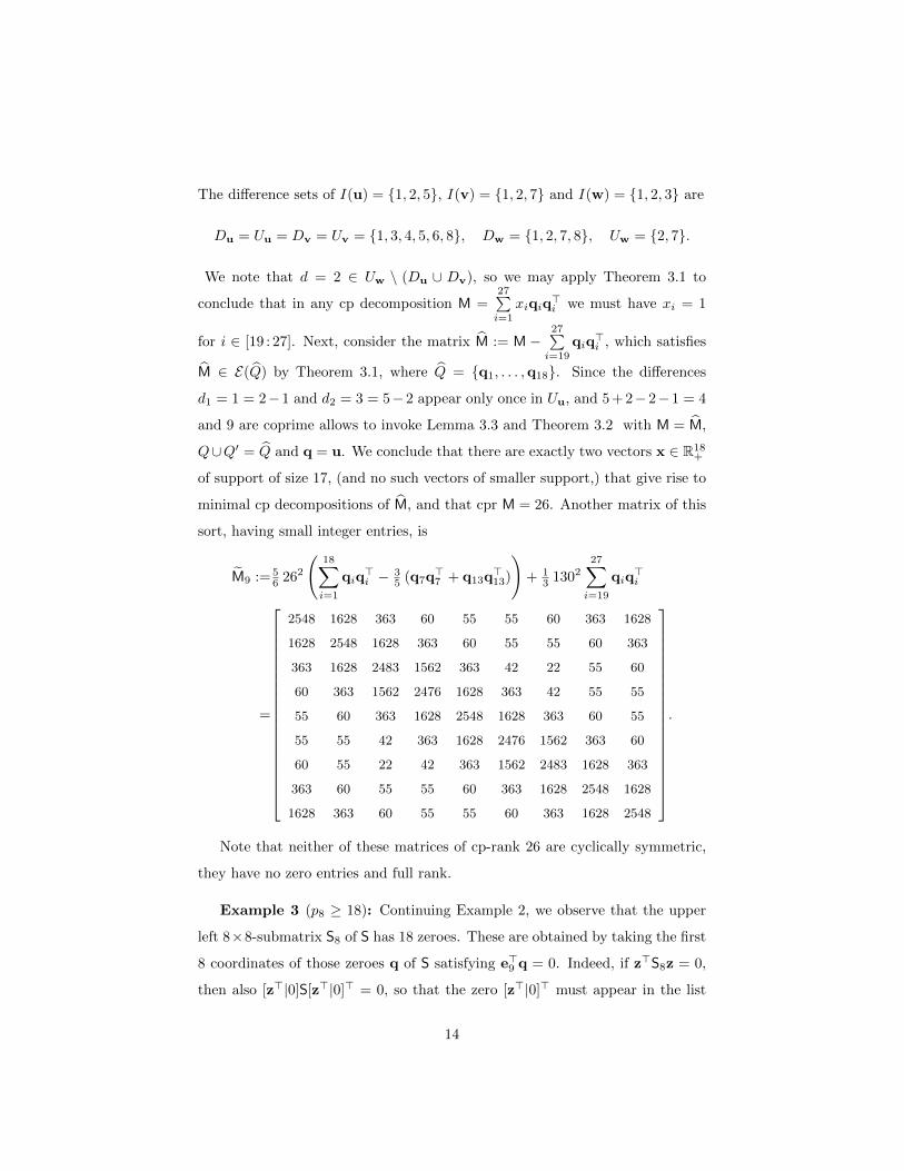
M ∈ E(Q) by Theorem 3.1, where Q = {q1, . . . ,q18}. Since the differences

d1 = 1 = 2−1 and d2 = 3 = 5−2 appear only once in Uu, and 5 + 2−2−1 = 4

and 9 are coprime allows to invoke Lemma 3.3 and Theorem 3.2 with M = M,

Q∪Q′ = Q and q = u. We conclude that there are exactly two vectors x ∈ R18+

of support of size 17, (and no such vectors of smaller support,) that give rise to

minimal cp decompositions of M, and that cpr M = 26. Another matrix of this

sort, having small integer entries, is

M9 := 56 262

(18∑i=1

qiq>i − 3

5 (q7q>7 + q13q

>13)

)+ 1

3 130227∑i=19

qiq>i

=

2548 1628 363 60 55 55 60 363 1628

1628 2548 1628 363 60 55 55 60 363

363 1628 2483 1562 363 42 22 55 60

60 363 1562 2476 1628 363 42 55 55

55 60 363 1628 2548 1628 363 60 55

55 55 42 363 1628 2476 1562 363 60

60 55 22 42 363 1562 2483 1628 363

363 60 55 55 60 363 1628 2548 1628

1628 363 60 55 55 60 363 1628 2548

.

Note that neither of these matrices of cp-rank 26 are cyclically symmetric,

they have no zero entries and full rank.

Example 3 (p8 ≥ 18): Continuing Example 2, we observe that the upper

left 8×8-submatrix S8 of S has 18 zeroes. These are obtained by taking the first

8 coordinates of those zeroes q of S satisfying e>9 q = 0. Indeed, if z>S8z = 0,

then also [z>|0]S[z>|0]> = 0, so that the zero [z>|0]> must appear in the list

14

of Example 2. Define the set S8 := {q ∈ {q1, . . . ,q27} : e>9 q = 0}. Then the

matrix M :=∑

q∈S8

qq> satisfies cpr M = 18, by Theorem 3.1, Lemma 3.3 and

Theorem 3.2. Moreover all entries in the last row and the last column of M are

zero, therefore also M8, the upper left 8× 8-submatrix of M, has cpr M8 = 18.

Again, by adjusting weights, we came up with a matrix with small integer

entries:

M8 :=

541 880 363 24 55 11 24 0

880 2007 1496 363 48 22 22 24

363 1496 2223 1452 363 24 22 11

24 363 1452 2325 1584 363 48 55

55 48 363 1584 2325 1452 363 24

11 22 24 363 1452 2223 1496 363

24 22 22 48 363 1496 2007 880

0 24 11 55 24 363 880 541

.

Note that M8 is, again, not cyclically symmetric, and that it has full rank.

Example 4 (p10 ≥ 27): Continuing Example 2, let M ∈ C10∗ be the matrix

obtained from M9 by appending a zero column o ∈ R9 and completing this to a

symmetric 10× 10 matrix by adding one row e>10 as the last one. Then, by [17,

Prop.2.2], we get

cpr M = cpr M9 + 1 = 27 .

Example 5 (p11 ≥ 32): Consider

S = C([32, 18, 4,−24,−31,−31,−24, 4, 18, 32, 32]>).

There are 33 zeroes of S; indeed, let

u = 121 [8, 0, 3, 0, 0, 0, 10, 0, 0, 0, 0]>

v = 121 [10, 0, 0, 0, 3, 0, 8, 0, 0, 0, 0]>

w = 17 [2, 0, 0, 2, 0, 0, 0, 3, 0, 0, 0]>

and define qi :=

Piu , if i ∈ [1 :11] ,

Piv , if i ∈ [12 :22] ,

Piw , if i ∈ [23 :33] ,

15

then the set of zeroes can be written as {qi : i ∈ [1 :33]}. Now put

M :=2

22∑i=1

qiq>i − q11q

>11 − q13q

>13 +

33∑i=23

qiq>i

= 1441

781 0 72 36 228 320 240 228 36 96 0

0 845 0 96 36 228 320 320 228 36 96

72 0 827 0 72 36 198 320 320 198 36

36 96 0 845 0 96 36 228 320 320 228

228 36 72 0 781 0 96 36 228 240 320

320 228 36 96 0 845 0 96 36 228 320

240 320 198 36 96 0 745 0 96 36 228

228 320 320 228 36 96 0 845 0 96 36

36 228 320 320 228 36 96 0 845 0 96

96 36 198 320 240 228 36 96 0 745 0

0 96 36 228 320 320 228 36 96 0 845

,

and again M has full rank. We get I(u) = {1, 3, 7}, I(v) = {1, 5, 7}, I(w) =

{1, 4, 8}, and we calculate

Du = Uu = Dv = Uv = {2, 4, 5, 6, 7, 9}, Dw = {3, 4, 7, 8}, Uw = {3, 8}.

Analogously to Example 2 we now show that the cp-rank is 32. Since d = 3 ∈

Uw \ (Du∪Dv), we must have xi = 1 for i ∈ [22 :33] by Theorem 3.1. Therefore

consider M := M −33∑i=22

qiq>i . We can see that the differences d1 = 6 = 7 − 1

and d2 = 4 = 7− 3 appear in Uu, and knowing that 7 + 3− 7− 1 = 2 and 11 are

coprime allows to invoke Lemma 3.3 and Theorem 3.2. Hence there are exactly

two vectors x ∈ R22+ of support of size 21 for M and this leads to a total of 32

for cpr M.

Table 1: (Ranges for) maximal cp-rank pn of cp matrices of order n.

n 5 6 7 8 9 10 11

dn 6 9 12 16 20 25 30

pn 6 ≤ 15 ≥ 14 ≥ 18 ≥ 26 ≥ 27 ≥ 32

sn 11 17 24 32 41 51 62

Table 1 summarizes the known bracket and consequences from above exam-

ples. A tighter upper bound p6 ≤ 15 was proved in [16, Thm.6.1], but up to

16

now no M ∈ C6∗ with cpr M > 9 = d6 is known.

Acknowledgment. The authors are indebted to an anonymous referee for

valuable suggestions which significantly improved presentation, and to Senior

Editor Raphael Loewy for his diligence in the evaluation process.

References

[1] Abraham Berman and Naomi Shaked-Monderer. Remarks on completely positive

matrices. Linear and Multilinear Algebra, 44:149–163, 1998.

[2] Abraham Berman and Naomi Shaked-Monderer. Completely positive matrices.

World Scientific Publishing Co. Inc., River Edge, NJ, 2003.

[3] Immanuel M. Bomze. Detecting all evolutionarily stable strategies. J. Optim.

Theory Appl., 75(2):313–329, 1992.

[4] Immanuel M. Bomze. Regularity versus degeneracy in dynamics, games, and

optimization: a unified approach to different aspects. SIAM Rev., 44(3):394–414,

2002.

[5] Immanuel M. Bomze. Copositive optimization – recent developments and appli-

cations. European J. Oper. Res., 216:509–520, 2012.

[6] Immanuel M. Bomze, Werner Schachinger, and Gabriele Uchida. Think

co(mpletely )positive ! – matrix properties, examples and a clustered bibliography

on copositive optimization. J. Global Optim., 52:423–445, 2012.

[7] Mark Broom, Chris Cannings, and Glenn T. Vickers. On the number of local

maxima of a constrained quadratic form. Proc. R. Soc. Lond. A, 443:573–584,

1993.

[8] Samuel Burer. Copositive programming. In Miguel F. Anjos and Jean Bernard

Lasserre, editors, Handbook of Semidefinite, Cone and Polynomial Optimization:

Theory, Algorithms, Software and Applications, International Series in Operations

Research and Management Science, pages 201–218. Springer, New York, 2012.

17

[9] Peter J. C. Dickinson, Mirjam Dur, Luuk Gijben, and Roland Hildebrand. Irre-

ducible elements of the copositive cone. Linear Algebra Appl., 439(6):1605–1626,

2013.

[10] John H. Drew and Charles R. Johnson. The no long odd cycle theorem for

completely positive matrices. In Random discrete structures, volume 76 of IMA

Vol. Math. Appl., pages 103–115. 1996.

[11] John H. Drew, Charles R. Johnson, and Raphael Loewy. Completely positive

matrices associated with M -matrices. Linear Multilinear Algebra, 37(4):303–310,

1994.

[12] Mirjam Dur. Copositive programming — a survey. In Moritz Diehl, Francois

Glineur, Elias Jarlebring, and Wim Michiels, editors, Recent Advances in Opti-

mization and its Applications in Engineering, pages 3–20. Springer, Berlin Hei-

delberg New York, 2010.

[13] Roland Hildebrand. The extremal rays of the 5×5 copositive cone. Linear Algebra

Appl., 437(7):1538–1547, 2012.

[14] Roland Hildebrand. Minimal zeros of copositive matrices. Preprint, http://

arxiv.org/abs/1401.0134, 2014.

[15] Raphael Loewy and Bit-Shun Tam. CP rank of completely positive matrices of

order 5. Linear Algebra Appl., 363:161–176, 2003.

[16] Naomi Shaked-Monderer, Abraham Berman, Immanuel M. Bomze, Florian Jarre,

and Werner Schachinger. New results on the cp rank and related properties

of co(mpletely )positive matrices. Linear Multilinear Algebra, to appear. Also

available at: arxiv.org/abs/1305.0737, 2013.

[17] Naomi Shaked-Monderer, Immanuel M. Bomze, Florian Jarre, and Werner

Schachinger. On the cp-rank and minimal cp factorizations of a completely posi-

tive matrix. SIAM J. Matrix Anal. Appl., 34(2):355–368, 2013.

18