arX

iv:h

ep-t

h/05

0520

6v2

3 J

un 2

005

Preprint typeset in JHEP style - PAPER VERSION BRX TH-567

hep-th/0505206

From Sasaki-Einstein spaces to quivers

via BPS geodesics: Lp,q|r

Sergio Benvenuti1, Martin Kruczenski2

1. Scuola Normale Superiore, Pisa,

and INFN, Sezione di Pisa, Italy.

2. Department of Physics, Brandeis University

Waltham, MA 02454, USA.

sergio.benvenuti@sns.it, martink@brandeis.edu.

Abstract: The AdS/CFT correspondence between Sasaki-Einstein spaces and quiver

gauge theories is studied from the perspective of massless BPS geodesics. The recently

constructed toric Lp,q|r geometries are considered: we determine the dual superconfor-

mal quivers and the spectrum of BPS mesons. The conformal anomaly is compared

with the volumes of the manifolds. The U(1)2F×U(1)R global symmetry quantum num-

bers of the mesonic operators are successfully matched with the conserved momenta

of the geodesics, providing a test of AdS/CFT duality. The correspondence between

BPS mesons and geodesics allows to find new precise relations between the two sides of

the duality. In particular the parameters that characterize the geometry are mapped

directly to the parameters used for a-maximization in the field theory.

The analysis simplifies for the special case of the Lp,q|q models, which are shown to

correspond to the known ”generalized conifolds”. These geometries can break conformal

invariance through toric deformations of the complex structure.

Keywords: AdS/CFT, quiver gauge theory, string theory.

Contents

1. Introduction 1

2. Strings moving in the Lp,q|rmanifold 4

2.1 A change of coordinates 5

2.2 R-charge 5

2.3 BPS geodesics 6

3. From GLSM charges to quivers and chiral rings: Lp,q|r 8

3.1 BPS mesons 14

4. Resolving the strip: Lp,q|q 16

4.1 Comparison with the geometry 19

5. General case: Lp,q|r 20

5.1 R-charges 20

5.2 The volume of the manifold 21

5.3 BPS operators and massless geodesics 22

6. Conclusions 23

7. Useful formulas 24

7.1 The geometry 24

7.2 Map to the field theory 26

1. Introduction

This paper studies the AdS/CFT correspondence [1] in the case of four dimensional

N = 1 gauge theories. Type IIB backgrounds of the form AdS5 ×X5, where X5 is a

Sasaki-Einstein manifold, are dual to a special class of superconformal gauge theories

called quivers. A quiver theory has product gauge group∏

SU(Ni) and the matter

fields transform in bifundamental representations. For superconformal quivers the two

gravitational central charges c and a are always equal and proportional to the inverse

– 1 –

of the volume of X5. The moduli space of vacua is of the form SymN(M3), where

M3 is the Calabi-Yau cone whose base is the Sasaki-Einstein X5. Another peculiar

feature of these no-flavor theories is the natural existence of long single-trace mesonic

operators, constructed from closed paths in the quivers, that are dual to semiclassical

strings moving in X5.

A special case of this is ”toric AdS/CFT”: the Calabi-Yau cone M3 is a toric

manifold, admitting three U(1) isometries. In other words X5 is a T 3 fibration over

a polygon, which is drawn on an integer two dimensional lattice. This small set of

discrete data (that can be encoded in the U(1) charges of the Gauged Linear Sigma

Model fields describing the toric cone) is enough to specify completely the full geometry,

and hence also the corresponding superconformal gauge theories. Of course, a more

explicit description, both of the geometries and of the gauge theories, is desirable. On

the geometric side, in particular, there is no known way to determine the toric Sasaki-

Einstein metric on X5 starting from the toric polygon. On the gauge side, the quiver

can be thought of as a more explicit description of the algebro-geometric structure of

the singularity M3, and an algorithm exists [3], even though it can efficiently handle

only small toric polygons; see [4, 5, 6, 7, 8, 10, 9].

Recently various work has been done in context of toric AdS/CFT, due to the

discovery of infinite sets of explicit Sasaki-Einstein metrics, in contrast to the previous

knowledge of only two examples, namely S5 and T 11. The latter case was analyzed by

Klebanov and Witten [2]. The study of these models led to many interesting results.

[11, 12, 13] found an infinite set of Sasaki-Einstein metrics on S2 × S3, called

Yp,q. These metrics are cohomogeneity one, the isometries being SU(2)× U(1)2. One

Abelian isometry, generated by the Reeb vector, is present in any, toric or not, Sasaki-

Einstein manifold and is dual to the R-symmetry of the gauge theory. In [14] the toric

description was found. The CY cones are quotients of C4; the four GLSM fields have

charges (p+ q, |p− q|;−p,−p). The Sasaki-Einstein spaces are smooth precisely when

p and q are coprime. Recently, a cohomogeneity-two generalization has been found

[15][16], leading to the so called Lp,q|r spaces. In fact, the same local metrics on the

Kahler-Einstein 4d base have been found some time ago in the mathematical literature

[17]. Moreover, in [17] these metrics are shown to be the most general orthotoric

Einstein metrics. The toric data of the Lp,q|r CY cones are a simple generalization of

the toric data of the Yp,q cones. There are still only four GLSM fields and a single U(1)

action, with integer charges (p, q;−r,−p− q + r)[15]. If p+ q = 2r one finds Y p,q.In [18], using the toric description of the singularities, the Yp,q superconformal

quivers have been constructed; a key role was played by the SU(2) global symmetry:

focusing on toric quivers with this non-Abelian flavor symmetry one is basically led

to the Yp,q quivers. Various checks of the correspondence can be performed [19, 18,

– 2 –

20, 21, 22]. Also the marginal deformations [23] match [24, 25]. A crucial role is

played by the technique of a-maximization [26], which relies on well established general

properties of supersymmetric theories [27, 26] and is thus valid for any 4d SCFT.

One, maybe surprising, feature of the Yp,q theories, that is important for the present

paper is the following: in the simpler Seiberg dual ”phases” of the theories, namely

the toric phases, there is a high degeneracy in the global symmetry quantum numbers

of the bifundamental fields. This can be understood to be necessary from the AdS

perspective: the smallest dibaryon operators have the same charges (modulo a factor

of N), and there are only a very small number of them, since they directly correspond

to the supersymmetric 3-cycles in the geometry.

We have recently witnessed a general progress in the algebro-geometric duality

between toric singularities and the gauge theories living on D3 branes probing the sin-

gularities: in [28] Hanany and Kennaway put forward a correspondence between the

toric data and the corresponding quivers. All toric quivers can be drawn on a torus pro-

viding a polygonalization of the torus; every superpotential term precisely corresponds

to a face. The dual graph of the quiver, the dimer, has a direct physical interpre-

tation in term of brane setups [29]. These setups significantly generalize previously

known constructions [32, 33, 34, 8]. In [30] many features of this picture have been

clarified and many examples have been given. The quiver/dimer ↔ toric Calabi-Yau’s

correspondence is part of a general framework [31] connecting statistical mechanics of

crystals and topological strings.

In [22] the periodic quiver picture was shown to encode naturally the mesonic

operators of the theories. In particular, the emergence of semiclassical strings directly

from paths in the periodic quivers was discussed: roughly speaking, the direction of a

long path on the quiver is mapped to the position of the string in the toric base of the

Sasaki-Einstein space. Massless BPS geodesic (i.e. point-like massless strings moving

only along the R-charge direction) are special cases of these, and turn out to encode a

great deal of information about the structure of the quiver.

The purpose of this paper is to show how the techniques of [22] can be extended

to generic examples of N = 1 AdS/CFT.

In section 2 we analyze the geometries, find the angle associated to the R-charge

and determine the properties of massless point-like strings moving along this direction,

that we call BPS geodesics.

Inspired by the results of [18] and [28], using the relation between the physical (p, q)-

webs of five branes and toric diagrams [35, 6], we then construct the superconformal

quivers associated to the Lp,q|rgeometries. An important role in the determination of

the global structure of the quivers is played by the mesonic BPS operators, that we

determine as in [22].

– 3 –

The main result of the present paper is a direct comparison between these BPS

mesons and BPS geodesics. As a warm up, in section 4 we discuss in detail this matching

for the special cases of Lp,q|q spaces. For these cases the gauge theories are known from

[36, 34] and the analysis is simpler and somewhat more transparent, both from the gauge

side and from the string side (the quartic equations in these cases become quadratic,

as for the Yp,qs). The end result is a non trivial matching of the U(1) × U(1) flavor

and U(1)R conserved charges between BPS geodesics and BPS mesons.

This comparison is than extended to a general Lp,q|rmodel in section 5. In this

section we also provide a direct relation between the parameters (α, β, xi) characterizing

the manifolds [15] and the parameters used in a-maximization [26].

2. Strings moving in the Lp,q|rmanifold

In this section we study point-like massless strings moving in the AdS5×Lp,q|r manifold

whose metric is [15]:

ds2 = −dt2 cosh2ρ+ dρ2 + sinh2ρ dΩ23 + ds2p,q|r (2.1)

ds2p,q|r = (dξ + σ)2 + ds2[4] (2.2)

where

ds2[4] =ρ2

4f(x)dx2 +

ρ2

h(θ)dθ2 +

f(x)

ρ2

(

sin2 θ

αdφ+

cos2 θ

βdψ

)2

(2.3)

+h(θ) sin2 θ cos2 θ

ρ2

(

(α− x)α

dφ− (β − x)β

dψ

)2

(2.4)

and

σ =(α− x) sin2 θ

αdφ+

(β − x) cos2 θβ

dψ (2.5)

f(x) = x(α − x)(β − x)− µ (2.6)

ρ2 = h(θ)− x (2.7)

h(θ) = α cos2 θ + β sin2 θ (2.8)

The geodesics we are interested in sit at the point ρ = 0 of AdS5 and move in the

internal manifold. Therefore in the rest of the paper we ignore the AdS5 part of the

background.

To study such geodesics we first do a change of coordinates and then properly

identify the angle conjugated to the R-charge. With that information we find the

relation between the conserved charges for some particular cases of interest which we

call extremal geodesics.

– 4 –

2.1 A change of coordinates

In order to facilitate the comparison between BPS geodesics and BPS mesons in the

gauge theory we redefine the variables by y = cos(2θ), getting

ds2[5] = (dξ + σ)2 + ds2[4] (2.9)

with

σ =(α− x)(1− y)

2αdφ+

(β − x)(1 + y)

2βdψ (2.10)

In such a way the two functions σi in dξ + σφdφ + σψdψ are products of two linear

functions of one coordinate on the toric base (x and y). This fact arises naturally when

comparing with the gauge theory.

The local Kahler-Einstein metric takes the fairly symmetric form

ds2[4] =ρ2

4f(x)dx2 +

f(x)

4ρ2

(

(1− y)α

dφ+(1 + y)

βdψ

)2

+ (2.11)

+ρ2

4g(y)dy2 +

g(y)

4ρ2

(

(α− x)α

dφ− (β − x)β

dψ

)2

(2.12)

with

f(x) = x(α− x)(β − x)− µ (2.13)

g(y) =1

2(α + β − y(α− β))(1− y2) (2.14)

ρ2 =1

2(α + β − y(α− β)− 2x) (2.15)

With α > β the ranges of the coordinates on the base is x1 ≤ x ≤ x2 and −1 ≤ y ≤ 1,

where 0 ≤ x1 ≤ x2 ≤ x3 are the three roots of f(x). Since x ≤ x2 ≤ β we have

ρ2 ≥ 12(α − β)(1 − y) ≥ 0, for y ≤ 1. Note also that g(y) is a cubic function of y as

f(x) is of x.

2.2 R-charge

To be able to compare the results for massless strings with the field theory side we

have to identify the angle conjugate to the R-symmetry. In order to do that, we need

to discuss briefly the computation of the holomorphic 3-form on the Calabi-Yau cone

Mp,q|r3 . This is because the holomorphic three form can be written as Ωijk = ηTΓijkη

with η the covariantly constant spinor. The R-charge rotates the covariantly constant

spinor as η → e12iαη and Ω→ eiαΩ.

– 5 –

With the 1-form σ defined in the four dimensional base of the Sasaki-Einstein

manifold, we compute its Kahler form k and complex structure J as:

k = −12dσ, J ba = kacg

cb, P ba =

1

2

(

δba + iJ ba)

(2.16)

where P ba projects out the anti holomorphic components. With this projector, we can

find two holomorphic 1-forms η1,2:

η1 =x− βf(x)

dx− 1 + y

g(y)dy +

2i

αdφ (2.17)

η2 =x− αf(x)

dx+1− yg(y)

dy +2i

βdψ (2.18)

(2.19)

The Sasaki-Einstein metric allows to construct a Calabi-Yau coneMp,q|r3 with metric

ds2 = dr2 + r2ds2[5] (2.20)

In this manifold we introduce a third holomorphic form

η3 =dr

r+ i (dξ + σ) (2.21)

Now, as argued by Martelli and Sparks in [16], the covariantly constant holomorphic

3-form follows as

Ω[3] =√

f(x)g(y) eiψR r3 η1 ∧ η2 ∧ η3 (2.22)

The phase ψR is conjugated to the R-charge and can be determined to be

ψR = 3ξ + φ+ ψ (2.23)

from the condition that Ω[3] should be covariantly constant.

We can therefore rewrite the 5d metric as

ds2[5] =

(

dψR3

+

(

(α− x)(1− y)2α

− 1

3

)

dφ+

(

(β − x)(1 + y)

2β− 1

3

)

dψ

)2

+ ds2[4]

(2.24)

2.3 BPS geodesics

The action for a massless particle moving along the internal manifold can be written

as

S =1

2

(1

3ψR + a1φ+ a2ψ)

2 + b1x2 + b2y

2 + (c1φ+ c2ψ)2 + (d1φ− d2ψ)2

(2.25)

– 6 –

with the definitions

a1 =(α− x)(1− y)

2α− 1

3, a2 =

(β − x)(1 + y)

2β− 1

3, b1 =

ρ2

4f(x), b2 =

ρ2

4g(y)(2.26)

c1 =

√

f(x)

2ρ

(1− y)α

, c2 =

√

f(x)

2ρ

(1 + y)

β, (2.27)

d1 =

√

g(y)

2ρ

(α− x)α

, d2 =

√

g(y)

2ρ

(β − x)β

(2.28)

We can compute the conjugate momenta:

PψR=

1

3

(

1

3ψR + a1φ+ a2ψ

)

(2.29)

Py = b2y (2.30)

Px = b1x (2.31)

Pφ = 3a1PψR+ c1(c1φ+ c2ψ) + d1(d1φ− d2ψ) (2.32)

Pψ = 3a2PψR+ c2(c1φ+ c2ψ)− d2(d1φ− d2ψ) (2.33)

and the Hamiltonian

H =9

2P 2ψR

+1

2b2P 2y +

1

2b1P 2x +

1

2(σ2

1 + σ22) (2.34)

where

σ1 = (c1φ+ c2ψ) (2.35)

σ2 = (d1φ− d2ψ) (2.36)

In terms of the momenta we get

σ1 = −−d2Pφ − d1Pψ + 3(a1d2 + a2d1)PψR

c1d2 + c2d1(2.37)

σ2 = −−c2Pφ + c1Pψ + 3(a1c2 − a2c1)PψR

c1d2 + c2d1(2.38)

(2.39)

Now we consider geodesics that satisfy Py = 0, Px = 0 implying that x = x0 and y = y0with x0 and y0 constant. These constants should be chosen so as to minimize H as

follows form the eq. of motion for x and y. The minimum is when σ1 = σ2 = 0, which

we expect to correspond to a BPS geodesic.

– 7 –

y x Pφ/PψRPψ/PψR

LD −1 x1 3(

23− x1

α

)

−1RU +1 x2 −1 3

(

23− x2

β

)

LU +1 x1 −1 3(

23− x1

β

)

RD −1 x2 3(

23− x1

α

)

−1

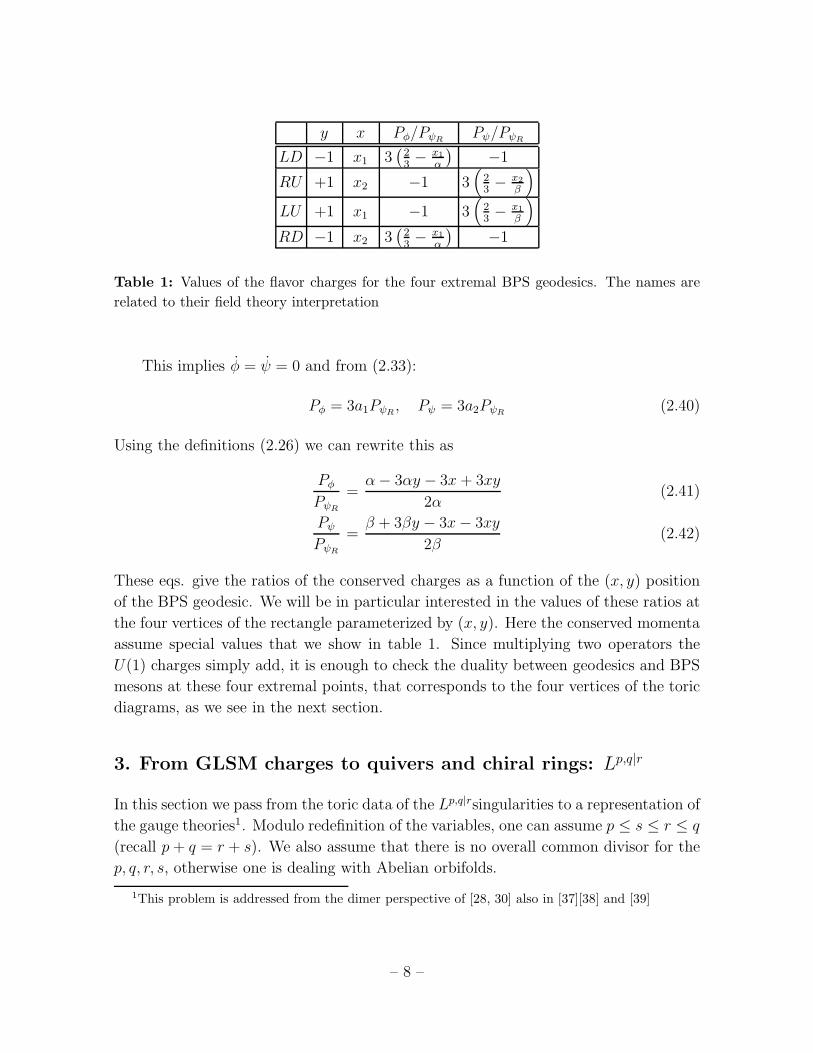
Table 1: Values of the flavor charges for the four extremal BPS geodesics. The names are

related to their field theory interpretation

This implies φ = ψ = 0 and from (2.33):

Pφ = 3a1PψR, Pψ = 3a2PψR

(2.40)

Using the definitions (2.26) we can rewrite this as

PφPψR

=α− 3αy − 3x+ 3xy

2α(2.41)

PψPψR

=β + 3βy − 3x− 3xy

2β(2.42)

These eqs. give the ratios of the conserved charges as a function of the (x, y) position

of the BPS geodesic. We will be in particular interested in the values of these ratios at

the four vertices of the rectangle parameterized by (x, y). Here the conserved momenta

assume special values that we show in table 1. Since multiplying two operators the

U(1) charges simply add, it is enough to check the duality between geodesics and BPS

mesons at these four extremal points, that corresponds to the four vertices of the toric

diagrams, as we see in the next section.

3. From GLSM charges to quivers and chiral rings: Lp,q|r

In this section we pass from the toric data of the Lp,q|rsingularities to a representation of

the gauge theories1. Modulo redefinition of the variables, one can assume p ≤ s ≤ r ≤ q

(recall p + q = r + s). We also assume that there is no overall common divisor for the

p, q, r, s, otherwise one is dealing with Abelian orbifolds.

1This problem is addressed from the dimer perspective of [28, 30] also in [37][38] and [39]

– 8 –

(1,0)

(a,p)

(0,−1)

(−s,b)

(p,1−a)

(s−p,a−b)

(0,0)

(b,s)

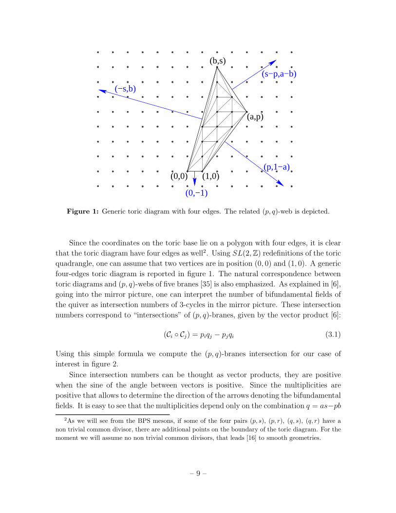
Figure 1: Generic toric diagram with four edges. The related (p, q)-web is depicted.

Since the coordinates on the toric base lie on a polygon with four edges, it is clear

that the toric diagram have four edges as well2. Using SL(2,Z) redefinitions of the toric

quadrangle, one can assume that two vertices are in position (0, 0) and (1, 0). A generic

four-edges toric diagram is reported in figure 1. The natural correspondence between

toric diagrams and (p, q)-webs of five branes [35] is also emphasized. As explained in [6],

going into the mirror picture, one can interpret the number of bifundamental fields of

the quiver as intersection numbers of 3-cycles in the mirror picture. These intersection

numbers correspond to “intersections” of (p, q)-branes, given by the vector product [6]:

(Ci Cj) = piqj − pjqi (3.1)

Using this simple formula we compute the (p, q)-branes intersection for our case of

interest in figure 2.

Since intersection numbers can be thought as vector products, they are positive

when the sine of the angle between vectors is positive. Since the multiplicities are

positive that allows to determine the direction of the arrows denoting the bifundamental

fields. It is easy to see that the multiplicities depend only on the combination q = as−pb2As we will see from the BPS mesons, if some of the four pairs (p, s), (p, r), (q, s), (q, r) have a

non trivial common divisor, there are additional points on the boundary of the toric diagram. For the

moment we will assume no non trivial common divisors, that leads [16] to smooth geometries.

– 9 –

(using SL(2,Z) redefinitions, one can assume a ≤ p). It is also convenient to define

r = p+q−s (implying p+q = r+s). The resulting bifundamentals together with their

multiplicities are depicted in figure 3. With our definitions, we are thus describing the

toric diagram corresponding to GLSM charges (p, q;−r,−p− q + r) [15]. p, q, r, s are

precisely the multiplicities of four of the type of the fields that have to appear in the

toric phases of the quiver. According to their direction, we call these four fields U ↑,D ↓, L← and R→.

Figure 3 should be thought of as the “folded” superconformal quiver. In other words

one can read off form that the number of the various types of fields and the number of

nodes. There are two additional diagonal fieldsտ andւ.3 This representation is very

useful in determining the global symmetry quantum numbers of the bifundamentals.

We call the two toric U(1) symmetries JH and JV , according to their orientation. The

values are reported in table 2.

Another way of finding the global symmetries from figure 3 is to associate a symme-

try to every of the four vertices, say Q1, . . . , Q4. The charges are +1 for bifundamentals

outgoing from that vertex, −1 for ingoing bifundamentals and 0 for the others. The

sum of these four symmetries vanishes, and a particular linear combination can be seen

to be the baryonic symmetry.4

The way to prove that all the field with the same direction have the same global

symmetry quantum number (recall however that they have different gauge quantum

numbers) is simply to impose the vanishing of the anomalies of these currents for each

node.

By studying the possible terms in the superpotential one concludes that the toric

representation of the quiver can be constructed using the blocks depicted in figure 5.

These block should be glued, respecting the orientation of the sides, into a fundamental

domain with a given number of each type. Finally it should be possible to draw the

fundamental domain on a torus (equivalently it should be possible to tile the plane with

it) giving rise to identifications between the points in the boundary of such domain.

This is better described with an example. In fig.6 and table 3 we give a construction

with na = 1, nb = 3, nc = 1.

In general, the number of blocks of type (a), (b) and (c) are: na = p, nb = q − s,3The picture we are proposing here is expected to be valid only for a subset of the toric phases. For

examples for the Yp,q in the so called “double impurity phases” there are also diagonal fields pointing

rightward [40].4In general the number of baryonic symmetries is equal to n− 3, where n is the number of external

(p, q)-branes. In our picture, for more generic toric diagrams, one constructs immediately n global

Abelian symmetries. The sum is always decoupled, two of them are the standard toric Abelian

isometries, and the remaining (n− 3) are the baryonic symmetries.

– 10 –

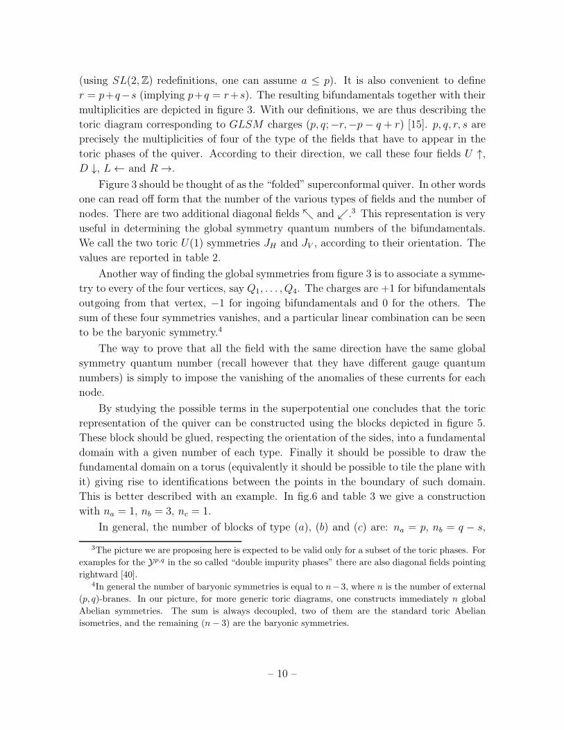
Field Number R0 QH QV Q3 QB

R → q 1 +1 0 0 +p

L ← p 1 −1 0 +1 +q

U ↑ s 0 0 +1 −1 −rD ↓ r 0 0 −1 0 −sտ q − s 1 −1 +1 0 q − rւ q − r 1 −1 −1 +1 q − s

Table 2: Charge assignments for the basic fields. The charge Q3 is redundant but plays a

role in the calculations. R0 is a trial R-charge which satisfies the same anomaly cancellation

constraints as the actual R-charge.

(s−p,a−b)

(p,1−a)

(0,−1)

(−s,b)

s−p as−bp

ps

as−bp−s

as−bp+p−s

Figure 2: Generic toric diagram with four edges. The intersection numbers are computed.

nc = q − r. The total number of nodes in the quiver is p + q, the total number

of bifundamental fields is p + 3q. This gives a total number of each type of field in

agreement with table 2.

Gluing these fundamental blocks gives rise to vertices of the type in figure 4. The

field theory interpretation is that each vertex corresponds to an SU(N) gauge group

and therefore implies anomaly cancellation conditions for the fields ending or emerging

– 11 –

r

s−p

p

s

q

q−s

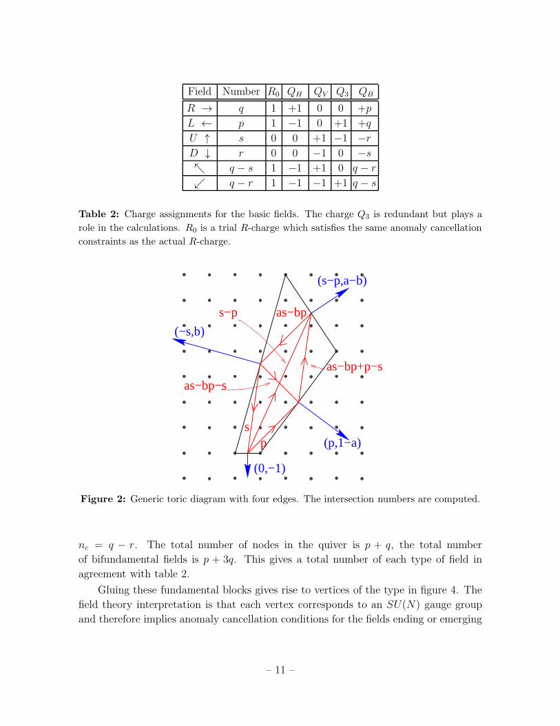
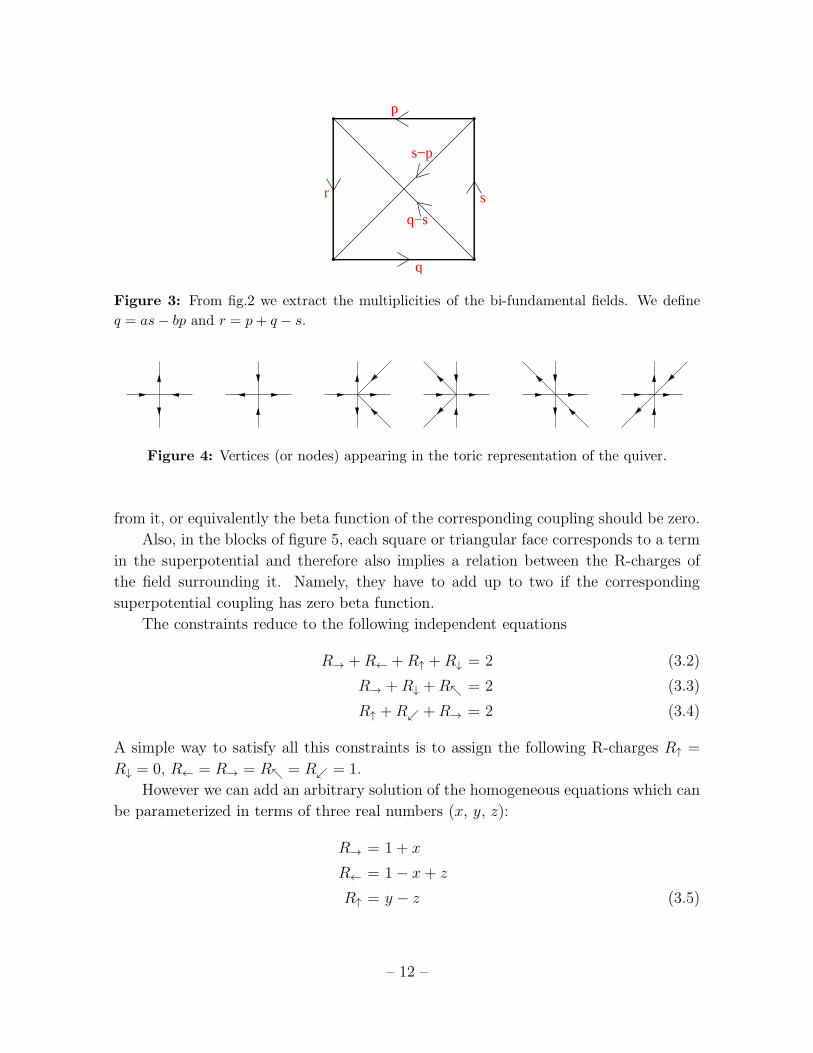
Figure 3: From fig.2 we extract the multiplicities of the bi-fundamental fields. We define

q = as− bp and r = p+ q − s.

Figure 4: Vertices (or nodes) appearing in the toric representation of the quiver.

from it, or equivalently the beta function of the corresponding coupling should be zero.

Also, in the blocks of figure 5, each square or triangular face corresponds to a term

in the superpotential and therefore also implies a relation between the R-charges of

the field surrounding it. Namely, they have to add up to two if the corresponding

superpotential coupling has zero beta function.

The constraints reduce to the following independent equations

R→ +R← +R↑ +R↓ = 2 (3.2)

R→ +R↓ +Rտ = 2 (3.3)

R↑ +Rւ +R→ = 2 (3.4)

A simple way to satisfy all this constraints is to assign the following R-charges R↑ =

R↓ = 0, R← = R→ = Rտ = Rւ = 1.

However we can add an arbitrary solution of the homogeneous equations which can

be parameterized in terms of three real numbers (x, y, z):

R→ = 1 + x

R← = 1− x+ z

R↑ = y − z (3.5)

– 12 –

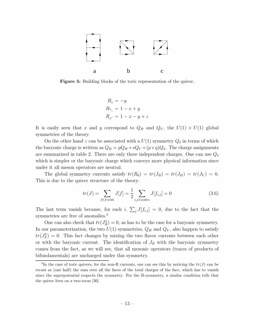
a b c

Figure 5: Building blocks of the toric representation of the quiver.

R↓ = −yRտ = 1− x+ y

Rւ = 1− x− y + z

It is easily seen that x and y correspond to QH and QV , the U(1) × U(1) global

symmetries of the theory.

On the other hand z can be associated with a U(1) symmetry Q3 in terms of which

the baryonic charge is written as QB = pQH+sQV +(p+q)Q3. The charge assignments

are summarized in table 2. There are only three independent charges. One can use Q3

which is simpler or the baryonic charge which conveys more physical information since

under it all meson operators are neutral.

The global symmetry currents satisfy tr(R0) = tr(JB) = tr(JH) = tr(JV ) = 0.

This is due to the quiver structure of the theory:

tr(J) =∑

f∈fields

J [f ] =1

2

∑

i,j∈nodes

J [fi,j] = 0 (3.6)

The last term vanish because, for each i,∑

j J [fi,j] = 0, due to the fact that the

symmetries are free of anomalies.5

One can also check that tr(J3B) = 0, as has to be the case for a baryonic symmetry.

In our parameterization, the two U(1) symmetries, QH and QV , also happen to satisfy

tr(J3F ) = 0. This fact changes by mixing the two flavor currents between each other

or with the baryonic current. The identification of JB with the baryonic symmetry

comes from the fact, as we will see, that all mesonic operators (traces of products of

bifundamentals) are uncharged under this symmetry.

5In the case of toric quivers, for the non-R currents, one can see this by noticing the tr(J) can be

recast as (one half) the sum over all the faces of the total charges of the face, which has to vanish

since the superpotential respects the symmetry. For the R-symmetry, a similar condition tells that

the quiver lives on a two-torus [30].

– 13 –

QV

QH

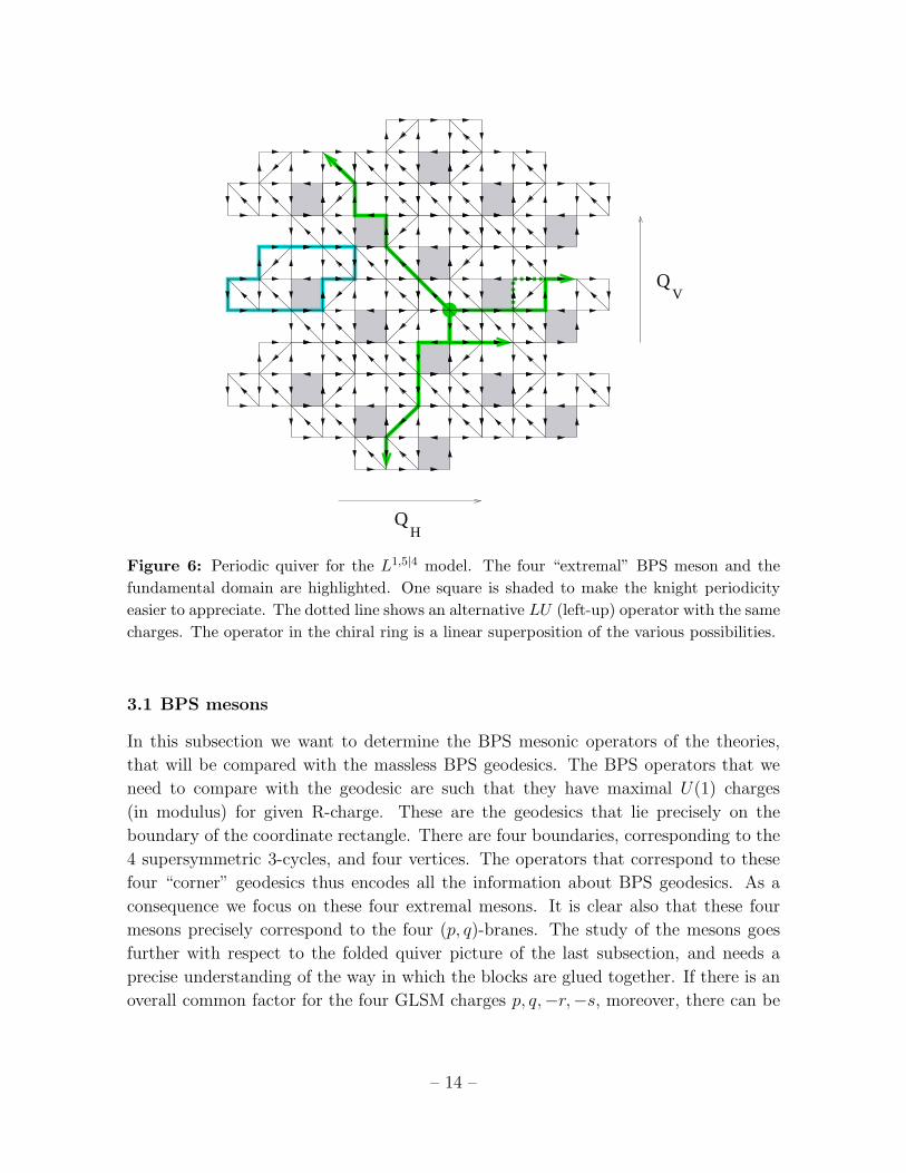
Figure 6: Periodic quiver for the L1,5|4 model. The four “extremal” BPS meson and the

fundamental domain are highlighted. One square is shaded to make the knight periodicity

easier to appreciate. The dotted line shows an alternative LU (left-up) operator with the same

charges. The operator in the chiral ring is a linear superposition of the various possibilities.

3.1 BPS mesons

In this subsection we want to determine the BPS mesonic operators of the theories,

that will be compared with the massless BPS geodesics. The BPS operators that we

need to compare with the geodesic are such that they have maximal U(1) charges

(in modulus) for given R-charge. These are the geodesics that lie precisely on the

boundary of the coordinate rectangle. There are four boundaries, corresponding to the

4 supersymmetric 3-cycles, and four vertices. The operators that correspond to these

four “corner” geodesics thus encodes all the information about BPS geodesics. As a

consequence we focus on these four extremal mesons. It is clear also that these four

mesons precisely correspond to the four (p, q)-branes. The study of the mesons goes

further with respect to the folded quiver picture of the last subsection, and needs a

precise understanding of the way in which the blocks are glued together. If there is an

overall common factor for the four GLSM charges p, q,−r,−s, moreover, there can be

– 14 –

various quivers corresponding to the same folded quiver. The simplest examples are the

two different Z2 quotients of the conifold. Assuming no overall common divisor there

is only one quiver; determining this gives also the global charges of our four extremal

BPS operators.

41

2

5 2

15 2 3

3 1 4

6

6 5

2 4

3 1

Table 3: The fundamental domain of L1,5|4 and the traditional quiver. The numbers identify

the six gauge groups and also determine how the fundamental domain is tiled to cover the

plane as in figure 6. Notice that whereas the quiver only contains the information about the

matter content of the theory, the periodic quiver, also tell the superpotential [28, 30].

Meson R0 R QH QV QB

OLD s −qy + s(1− x+ z) −s −q 0

ORU r r(1 + x) + p(y − z) +r +p 0

OLU r r(1− x+ z) + q(y − z) −r +q 0

ORD s s(1 + x)− py +s −p 0

Table 4: Charge assignments for the four extremal BPS mesons. The variables (x, y, z) are

taken at the local maximum of the central charge a.

The extremal operator going in the right-up direction, ORU , for instance, is com-

posed of → and ↑ fields. The extremal operator going in the left-up direction, OLUis composed only of ←, ↑ and տ fields. Similarly for the other two operators. These

requirements uniquely determine the four operators.

Without entering into the details, the end result is pretty simple. We assume for

the moment that gcd(p, s) = gcd(p, r) = gcd(q, s) = gcd(q, r) = 1 and summarize

the general results in table 4. As an explicit example, in figure 6 we depict the four

extremal operators for the particular case of L1,5|4.

– 15 –

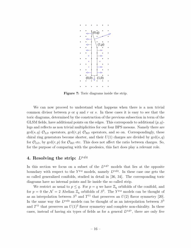
(0,q)

(1,p)

(0,0) (1,0)

Figure 7: Toric diagrams inside the strip.

We can now proceed to understand what happens when there is a non trivial

common divisor between p or q and r or s. In these cases it is easy to see that the

toric diagrams, determined by the construction of the previous subsection in term of the

GLSM fields, have additional points on the edges. This corresponds to additional (p, q)-

legs and reflects as non trivial multiplicities for our four BPS mesons. Namely there are

gcd(s, q) OLD operators, gcd(r, p) ORD operators, and so on. Correspondingly, these

chiral ring generators become shorter, and their U(1) charges are divided by gcd(s, q)

for OLD, by gcd(r, p) for ORD etc. This does not affect the ratio between charges. So,

for the purpose of comparing with the geodesics, this fact does play a relevant role.

4. Resolving the strip: Lp,q|q

In this section we focus on a subset of the Lp,q|r models that lies at the opposite

boundary with respect to the Y p,q models, namely Lp,q|q. In these case one gets the

so called generalized conifolds, studied in detail in [36, 34]. The corresponding toric

diagrams have no internal points and lie inside the so called strip.

We restrict as usual to p ≤ q. For p = q we have Zq orbifolds of the conifold, and

for p = 0 the N = 2 Abelian Zq orbifolds of S5. The Y p,q models can be thought of

as an interpolation between S5 and T 11 that preserves an U(2) flavor symmetry [20].

In the same way the Lp,q|q models can be thought of as an interpolation between S5

and T 11 that preserves an U(1)2 flavor symmetry and complete non-chirality. In these

cases, instead of having six types of fields as for a general Lp,q|r, there are only five

– 16 –

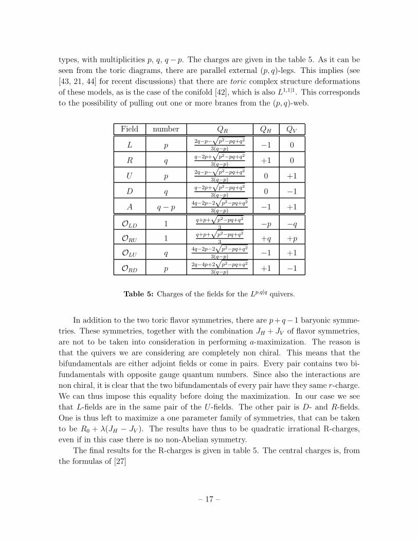
types, with multiplicities p, q, q− p. The charges are given in the table 5. As it can be

seen from the toric diagrams, there are parallel external (p, q)-legs. This implies (see

[43, 21, 44] for recent discussions) that there are toric complex structure deformations

of these models, as is the case of the conifold [42], which is also L1,1|1. This corresponds

to the possibility of pulling out one or more branes from the (p, q)-web.

Field number QR QH QV

L p2q−p−

√p2−pq+q2

3(q−p)−1 0

R qq−2p+

√p2−pq+q2

3(q−p)+1 0

U p2q−p−

√p2−pq+q2

3(q−p)0 +1

D qq−2p+

√p2−pq+q2

3(q−p)0 −1

A q − p 4q−2p−2√p2−pq+q2

3(q−p)−1 +1

OLD 1q+p+√p2−pq+q2

3−p −q

ORU 1q+p+√p2−pq+q2

3+q +p

OLU q4q−2p−2

√p2−pq+q2

3(q−p)−1 +1

ORD p2q−4p+2

√p2−pq+q2

3(q−p)+1 −1

Table 5: Charges of the fields for the Lp,q|q quivers.

In addition to the two toric flavor symmetries, there are p+ q−1 baryonic symme-

tries. These symmetries, together with the combination JH + JV of flavor symmetries,

are not to be taken into consideration in performing a-maximization. The reason is

that the quivers we are considering are completely non chiral. This means that the

bifundamentals are either adjoint fields or come in pairs. Every pair contains two bi-

fundamentals with opposite gauge quantum numbers. Since also the interactions are

non chiral, it is clear that the two bifundamentals of every pair have they same r-charge.

We can thus impose this equality before doing the maximization. In our case we see

that L-fields are in the same pair of the U -fields. The other pair is D- and R-fields.

One is thus left to maximize a one parameter family of symmetries, that can be taken

to be R0 + λ(JH − JV ). The results have thus to be quadratic irrational R-charges,

even if in this case there is no non-Abelian symmetry.

The final results for the R-charges is given in table 5. The central charges is, from

the formulas of [27]

– 17 –

q−p p

Figure 8: A toric phase for the generalized conifold. We show in the dotted lines how to

glue the fundamental domain.

c = a =9

32tr(R3) =

2p3 − 3p2q − 3pq2 + 2q3 + 2√

(p2 − pq + q2)3

16(q − p)2 (4.1)

The AdS/CFT formula [1, 41] a = π3

4Vrelates this central charge to the volume of

the Lp,q|q manifold. The result for the volumes is given in [15] in terms of the solutions

of a quartic equation. It is easy to see that such equation becomes quadratic in the

case p = s, q = r and the positive solution matches precisely the field theory result.

It is important that the results obtained so far in this section can be applied to

different quivers, if q and p are not coprime integers. This corresponds to the possibility

of taking different Zk orbifolds of the same toric Sasaki-Einstein manifold. In this case

the chiral ring generators can be different from the ones we discuss. We thus restrict

to q and p coprime. In this case there is only one quiver, modulo Seiberg dualities.

The chiral ring is generated by four different types of operators. One subtlety is that

some of these operators come with non trivial multiplicities, this is due to the non

smoothness of the background. From the (p, q)-web of 5 branes (corresponding directly

to the toric diagrams) this fact can be seen as the presence of parallel external legs. It

is the analog of the presence of two L− operators with spin 0 in Y p,p [22].

There are two long operators, one, OLD, made of p L-fields and q D–fields and one,

ORU , made of p U -fields and q R-fields. There are q − p length 1 operators made with

the q − p different adjoint A-fields, that come together with the p mesons of the form

– 18 –

tr(UL). Finally, we find p length 2 of the form tr(DR).

Now we redefine the two flavor charges QH and QV in such a way that for each

meson one of the two new charges, that we call Qφ and Qψ, satisfy Qφ = −QR or

Qψ = −QR. We display the charges in table 6. This gauge theoretical table is meant

Meson QH QV Qφ/QR Qψ/QR

OLD −p −q −1 p+2q−2√p2−pq+q2

p

ORU +q +p2p+q−2

√p2−pq+q2

q−1

OLU −1 +1−p+q+

√p2−pq+q2

q−1

ORD +1 −1 −1 p−q+√p2−pq+q2

p

Table 6: Charge assignments for the four extremal mesonic fields.

to be compared with the geometrical table 1 of section 2. By construction the (−1)s inthe last two columns match. We now compute the other four values from the geometry.

4.1 Comparison with the geometry

In the case of r = q the geometrical formulas of the Appendix simplify. Eqs. (7.9) and

(7.8) become

0 = p− 4qχ1 − 4(p− q)χ21 (4.2)

χ1 + χ2 =1

2(4.3)

which give

χ1 =−p +

√

p2 − pq + q2

2(q − p) (4.4)

χ2 =q −

√

p2 − pq + q2

2(q − p) (4.5)

Due to eq. (4.3), the square root in eq. (7.10) simplifies to√

1− 2(χ1 + χ2) + (χ2 − χ1)2 = χ2 − χ1 ≥ 0 (4.6)

We thus find

2

3− x1α

=p+ 2q − 2

√

p2 − pq + q2

3p(4.7)

– 19 –

2

3− x2α

=p− q +

√

p2 − pq + q2

3p(4.8)

2

3− x1

β=q − p+

√

p2 − pq + q2

3q(4.9)

2

3− x2

β=q + 2p− 2

√

p2 − pq + q2

3q(4.10)

These are precisely the values found on the gauge side, reported in Table 6.

5. General case: Lp,q|r

5.1 R-charges

In this section we perform a-maximization [26] to obtain the R-charges and compare

to the previous results. As a check we also compare the central charge we obtain to

the volume of the Sasaki-Einstein manifold.

Given the charge assignments of table 2 and eq.(3.5), the a-function that we should

maximize can be written as

tr((R− 1)3) =32

9a = p+ q + qx3 + p(z − x)3 + s(y − z − 1)3

+r(−y − 1)3 + (q − s)(y − x)3 + (q − r)(z − x− y)3 (5.1)

where we included the contribution p + q from the gauginos. Now we have to find

the point at which ∂xa = ∂ya = ∂za = 0. It is useful to introduce two new variables

ξ1 = x/z and ξ2 = y/z. The first equations to solve implies

∂a

∂x= 0 ⇐⇒ ξ1 =

1

2

s+ 2(r − q)ξ2 + (q − p)ξ22s+ (r − s)ξ2

(5.2)

Then we get

s∂a

∂y+ (s− r)∂a

∂z= 0 ⇐⇒ (5.3)

z =2rs(1− 2ξ2)

p(s− r)ξ22 + 2ξ1ξ2(q(r + s)− s2 − r2) + 2prξ2 + 2s(p− r)ξ1 − sp(5.4)

Finally, replacing the expressions for z and ξ1 in the equation ∂a∂z

= 0 we get a quartic

equation for ξ2:

P[4](ξ2) = 0 (5.5)

– 20 –

where P[4] is a polynomial of order four given by

P[4](ξ2) = 4(−4r2−p2+ + p2+p2− + 3r4−) ξ

42 (5.6)

+(32r2−p2+ + 4r−p+p

2− + 12r3−p+ − 24r4− − 8p2+p

2− − 16r−p

3+) ξ

32

+(r2−p2− + 19r4− − 21r2−p

2+ − 6r−p+p

2− − 18r3−p+ − 4p4+ + 5p2+p

2− + 24r−p

3+) ξ

22

+(10r3−p+ − r2−p2− − p2+p2− − 7r4− − 12r−p3+ + 5r2−p

2+ + 4p4+ + 2r−p+p

2−) ξ2

+r4− − p4+ + 2r−p3+ − 2r3−p+

where, for brevity we defined p± = p ± q and r− = r − s. When r = s or p = r

corresponding to r− = 0 or r− = p−, the equation factorizes. In the r− = 0 case, which

corresponds to Y12p+,−

12p−, a solution is ξ2 = 1

2which can be seen to agree with the

known result.

5.2 The volume of the manifold

A way to check the a-maximization we performed is to compute a and compare with

the volume of the Lp,q|r manifold. The value of a at the local maximum can be seen to

be632

9a = r + s− r(1 + y)2 − s(1− y + z)2 (5.7)

where the bars indicate quantities evaluated at the local maximum. We can now obtain

an expression in terms of ξ2:

a = −18 p q rs ξ2(ξ2 − 1)(2ξ2 − 1)[p+ + r−(2ξ2 − 1)]2[r− + p+(2ξ2 − 1)]

P (ξ2)2(5.8)

P (ξ2) = 4p+(r2− − p2−) ξ32 + 2

[

2r3− − r−(p2+ + p2−)− 3p+(r2− − p2−)

]

ξ22 (5.9)

+2(p+ − r−)(2r2− − p2− − p2+) ξ2 + (p+ + r−)(p+ − r−)2 (5.10)

We can rewrite a in terms of a variable W as

a =1

4

8pqrs

(p+ q)31

W(5.11)

Since ξ2 obeys the quartic equation (5.5) that implies that W also satisfies a similar

equation. Using a computer algebra program (e.g. Maple or Mathematica), it is easy

to check that the equation W satisfies is7:

0 = (1− f 2)(1− g2)h4− + 2h2−[

2 (2− h+)2 − 3h2−]

W (5.12)6This result is obtained by computing a = a− 1

3 (x∂xa+ y∂ya+ z∂za) which at the extremes agrees

with a.7To check this, one replaces (5.10) in this equation. After taking common denominator the numer-

ator can be seen to factorize into P[4](ξ2) and a polynomial of order twenty. Since, by (5.5), P[4](ξ2)=0,

the equation is satisfied.

– 21 –

[

8h+ (2− h+)2 − h2−(30 + 9h+)]

W 2 (5.13)

+6(2− 9h+)W3 − 27W 4 (5.14)

where f = −p−/p+, g = r−/p+ and h± = f 2 ± g2. This equation is precisely the same

equation that appeared in [15] and determines the volume V = π3(p + q)3W/(8pqrs)

of the Lp,q|r manifold. This implies that the AdS/CFT relation [1, 41]

a =π3

4V(5.15)

between a and the volume V of the manifold is exactly satisfied. It is perhaps interesting

that even if only one solution of the quartic equation for the volume is physical all

solutions actually match. This suggest that it might be possible to do a more direct

derivation of the equivalence between the supergravity and field theory computations.

5.3 BPS operators and massless geodesics

Now we would like to compare the flavor and R-charges of the operators that we

associate with the geodesics at the “corners” of the geometry and that we summarized

in table 1. The charges of the corresponding operators are summarized in table 4. One

thing to note is that since Rւ = R↓ +R← and Rտ = R↑ +R← then the R-charges of

these particular operators depend only on their total QH and QV charges. For other

operators that is not the case, for example there are operators with large R-charge and

QH = QV = 0, that arise taking powers of one basic operator Oβ with QR = 2 and

QH = QV = 0. This short BPS meson Oβ generates the β-deformation [24, 25] and

exists for any toric superconformal quiver [24].

Our first task is to relate the U(1) flavor charges QV and QH with the isometries

Qφ and Qψ of the background. We found that we obtain a correct matching if we define

QV =1

2(Qψ −Qφ) (5.16)

QH = −(AQφ +BQψ)

2 p q (x2 − x1)(5.17)

A = ps(α− x1) + qs(α− x2) (5.18)

B = pr(β − x1) + qr(β − x2) (5.19)

The R-charges of the operators can be computed from eqn. (3.5) (see table 4), with

the result

RLD = −qy + s(1− x+ z) (5.20)

RRU = r(1 + x) + p(y − z) (5.21)

RLU = r(1− x+ z) + q(y − z) (5.22)

RRD = s(1 + x)− py (5.23)

– 22 –

We remind the reader that (x, y, z) indicates (x, y, z) evaluated at the local maximum

of the central charge a. For the ratios QV /QR and QH/QR to match between field

theory and supergravity background we need that

−32

(

1− x1α

)

=−q

−qy + s(1− x+ z)(5.24)

3

2

(

1− x2β

)

=p

r(1 + x) + p(y − z) (5.25)

3

2

(

1− x1β

)

=q

r(1− x+ z) + q(y − z) (5.26)

−32

(

1− x2α

)

=−p

−py + s(1 + x)(5.27)

In the appendix we show that these relations are exactly valid. In fact, together with

a further relation

x3α

= − 2

3y(5.28)

x3β

=2

3(y − z) (5.29)

can be used to compute all parameters of the geometry in terms of field theory quan-

tities. We emphasize that these simple relations were found thanks to the method of

comparing massless geodesics with BPS operators.

6. Conclusions

In the present paper we consider massless geodesics moving in the recently found Lp,q|r

backgrounds. The study of the geodesics give considerable information about the field

theory, in particular they determine a set of four operators which have maximal charges

(in modulus) for given R-charge. These are operators which are constituted by elemen-

tary fields all with the same sign of each charge. We find four of them, in correspon-

dence with the signs of the two flavor charges. On the other hand an analysis of the

toric diagrams of the theories and comparison with the previously known Yp,q case

suggest a generic construction of the toric representation of the quiver. This allows

us to conjecture the generic superconformal theories dual to the Lp,q|r manifolds. For

those theories we compute the R-charges using a-maximization and find that the re-

sult precisely matches the computation done in the geometry. In particular a precise

mapping is found between the parameters of the geometry and those that arise in the

field theory when performing a-maximization. The analysis is straight-forward albeit

– 23 –

cumbersome. For that reason we choose an example of interest, the so called “general-

ized conifolds” which can be identified with Lp,q|q. In that case we compute explicitly

all the R-charges. In the generic case the results are written in terms of the solutions

of a quartic equation on both sides of the correspondence. The agreement is shown by

verifying that the solutions on one side satisfy the equations on the other side of the

correspondence.

In further work, it would be interesting to do a study of extended semiclassical

strings [45] in these backgrounds, as was done in [22] for the Yp,q case.It would also be interesting to see if there is a way of finding the properties of

geodesics starting directly from the toric diagrams. A similar understanding has been

achieved for the volumes in [46].

Acknowledgments

We would like to thank Amihay Hanany for many interesting and enjoyable conversa-

tions. We are also grateful to Sebastian Franco, Pavlos Kazakopoulos, Matt Strassler,

David Vegh, Brian Wecht and Alberto Zaffaroni for discussions. S.B. has benefited of

the warm hospitality of MIT while this work was being done. M.K. wants to thank the

University of Washington for hospitality while part of this work was being done. The

work of M. K. is supported in part by NSF through grants PHY-0331516, PHY99-73935

and DOE under grant DE-FG02-92ER40706.

7. Useful formulas

7.1 The geometry

The manifold Lp,q|r is defined in terms of two different sets of parameters. One is (α,

β) and the roots x1 < x2 < x3 of the cubic equation x(α − x)(β − x) = µ. The other

are the integers p,q,r. Here we are interested in an explicit relation between the two

sets that we derive following [15].

The roots x1,2,3 satisfy (we assume from now on µ = 1)

x1x2x3 = 1, x1x2 + x1x3 + x2x3 = αβ, x1 + x2 + x3 = α + β (7.1)

From [15], the relation to the integers p,q,r is given through a set of parameters Ai, Bi

, Ci, i = 1, 2 defined as

Ai =αCixi − α

, Bi =βCixi − β

, Ci =(α− xi)(β − xi)

2(α + β)xi − αβ − 3x2i(7.2)

– 24 –

and which satisfy

pC1 + qC2 = 0, pA1 + qA2 + r = 0, pB1 + qB2 + s = 0 (7.3)

Using eq. (7.1) we can write

C1 = −1

x1(x1 − x2)(x1 − x3), C2 = −

1

x2(x2 − x1)(x2 − x3)(7.4)

We can derive now two equations relating the xi’s to the integers p,q,r:

px2(x2 − x3) = qx1(x1 − x3), x1x2 + x1x3 + x2x3 =rs

pq(x1 − x3)(x2 − x3) (7.5)

which together with x1x2x3 = 1 completely determine xi in terms of p,q,r. To solve

these equations we introduce the ratios

χ1 =x1x3, χ2 =

x2x3

(7.6)

The equations now reduce to

pχ2(1− χ2) = qχ1(1− χ1), χ1χ2 + χ1 + χ2 =rs

pq(1− χ1)(1− χ2) (7.7)

The second equation allows to obtain χ2 as:

χ2 =−p q χ1 + rs (1− χ1)

p q (1 + χ1) + rs (1− χ1)(7.8)

Replacing in the first one, we find a quartic equation for χ1:

0 = (p q − rs)2χ41 + (p q − rs) (3rs+ p q)χ3

1 (7.9)

+(p q + rs) (3rs− 2p2 − p q)χ21 + [p2(rs− p q)− (p q + rs)2]χ1 + p2rs

The other parameters follow trivially as

x1 =

(

χ21

χ2

)13

, x2 =

(

χ22

χ1

)13

, x3 =1

(χ1χ2)13

(7.10)

α =1 + χ1 + χ2 +

√

1− 2χ1 + χ21 − 2χ2 + χ2

2 − 2χ1χ2

2(χ1χ2)13

(7.11)

β =1 + χ1 + χ2 −

√

1− 2χ1 + χ21 − 2χ2 + χ2

2 − 2χ1χ2

2(χ1χ2)13

(7.12)

– 25 –

We finally write

xiα

=2χi

1 + χ1 + χ2 +√

1− 2χ1 + χ21 − 2χ2 + χ2

2 − 2χ1χ2

(7.13)

xiβ

=2χi

1 + χ1 + χ2 −√

1− 2χ1 + χ21 − 2χ2 + χ2

2 − 2χ1χ2

(7.14)

from which it possible to find the value of the U(1)-fibration functions at the four

vertices of the coordinate rectangle. Note that, although we set µ = 1, the results for

any ratio of two of the quantities xi, α, β is independent of µ.

7.2 Map to the field theory

Now we want to find the relation between the parameters xi=1...3, α, β in the geometry

and those in the field theory. The parameters we consider in the field theory are

x, y, z used in section 5, when performing a-maximization. Here we consider them

always evaluated at the local maximum in which case they are functions of p, q and

r as determined in that section. To emphasize that they are evaluated at the local

maximum we denote them as x, y and z.

Analyzing the matching to massless geodesics we were led to certain relations that

can be summarized as follows:

ζ1 =x1α

= 1 +2

3

q

qy − s(1− x+ z)(7.15)

ζ2 =x2α

= 1 − 2

3

p

−py + s(1 + x)(7.16)

ζ3 =x3α

= − 2

3

1

y(7.17)

ζ1 =x1β

= 1 − 2

3

q

q(y − z) + r(1− x+ z)(7.18)

ζ2 =x2β

= 1 − 2

3

p

p(y − z) + r(1 + x)(7.19)

ζ3 =x3β

=2

3

1

y − z (7.20)

It is easier, as we did, to write these relations in terms of ratios. In the geometry this

amounts to eliminating the parameter µ. To prove these relations, we proceed to show

that they satisfy the same equations that we derived in the previous subsection (after

appropriately dividing by α and eliminating β/α:

p ζ2 (ζ2 − ζ3) = q ζ1 (ζ1 − ζ3) (7.21)

– 26 –

ζ1ζ2 + ζ1ζ3 + ζ2ζ3 =rs

p q(ζ1 − ζ3)(ζ2 − ζ3) (7.22)

ζ1 + ζ2 + ζ3 = 1 + ζ1ζ2 + ζ1ζ3 + ζ2ζ3 (7.23)

To check these equations first one replaces x, y and z by their expressions in terms

of ξ2, namely following eqs. (5.2), (5.4). After that, the equation becomes a rational

function whose numerator is a polynomial multiple of P[4](ξ2) as defined in (5.6). Since,

at the local extrema, ξ2 is a root of P[4](ξ2), the equations are satisfied.

These equation completely determine ζi=1...3 up to a discrete set of permutations.

We checked using particular examples that the assignments are as we discussed in the

case r > s that we are considering.

The same applies to the ζi=1...3. Moreover, as an exercise, one can check that other

relations such as ζ1ζ2 − ζ1ζ2 = 0 also reduce to zero after using that P[4](ξ2) = 0.

References

[1] J. Maldacena, “The large N limit of superconformal field theories and supergravity,”

Adv. Theor. Math. Phys. 2, 231 (1998) [Int. J. Theor. Phys. 38, 1113 (1998)],

hep-th/9711200,

S. S. Gubser, I. R. Klebanov and A. M. Polyakov, “Gauge theory correlators from

non-critical string theory,” Phys. Lett. B 428, 105 (1998), [arXiv:hep-th/9802109],

E. Witten, “Anti-de Sitter space and holography,” Adv. Theor. Math. Phys. 2, 253

(1998), [arXiv:hep-th/9802150],

O. Aharony, S. S. Gubser, J. M. Maldacena, H. Ooguri and Y. Oz, “Large N field

theories, string theory and gravity,” Phys. Rept. 323, 183 (2000)

[2] I. R. Klebanov and E. Witten, “Superconformal field theory on three-branes at a

Calabi-Yau singularity,” Nucl. Phys. B 536:199-218,1998. arXiv:hep-th/9807080

[3] B. Feng, A. Hanany and Y. H. He, “D-brane gauge theories from toric singularities and

toric duality,” Nucl. Phys. B 595, 165 (2001). arXiv:hep-th/0003085.

[4] D. R. Morrison and M. R. Plesser, “Non-spherical horizons. I,” Adv. Theor. Math.

Phys. 3, 1 (1999) [arXiv:hep-th/9810201].

[5] C. Beasley, B. R. Greene, C. I. Lazaroiu and M. R. Plesser, “D3-branes on partial

resolutions of abelian quotient singularities of Calabi-Yau threefolds,” Nucl. Phys. B

566, 599 (2000) [arXiv:hep-th/9907186].

[6] A. Hanany and A. Iqbal, “Quiver theories from D6-branes via mirror symmetry,”

JHEP 0204, 009 (2002) [arXiv:hep-th/0108137].

– 27 –

[7] C. E. Beasley and M. R. Plesser, “Toric duality is Seiberg duality,” JHEP 0112, 001

(2001) [arXiv:hep-th/0109053].

[8] B. Feng, A. Hanany, Y. H. He and A. M. Uranga, “Toric duality as Seiberg duality and

brane diamonds,” JHEP 0112, 035 (2001) [arXiv:hep-th/0109063].

[9] B. Feng, S. Franco, A. Hanany and Y. H. He, “Symmetries of toric duality,” JHEP

0212, 076 (2002) [arXiv:hep-th/0205144].

[10] B. Feng, A. Hanany, Y. H. He and A. Iqbal, “Quiver theories, soliton spectra and

Picard-Lefschetz transformations,” JHEP 0302, 056 (2003) [arXiv:hep-th/0206152].

[11] J. P. Gauntlett, D. Martelli, J. Sparks and D. Waldram, “Supersymmetric AdS(5)

solutions of M-theory,” Class. Quant. Grav. 21, 4335 (2004) [arXiv:hep-th/0402153].

[12] J. P. Gauntlett, D. Martelli, J. Sparks and D. Waldram, “Sasaki-Einstein metrics on

S(2) x S(3),” arXiv:hep-th/0403002.

[13] J. P. Gauntlett, D. Martelli, J. F. Sparks and D. Waldram, “A new infinite class of

Sasaki-Einstein manifolds,” arXiv:hep-th/0403038.

[14] D. Martelli and J. Sparks, “Toric geometry, Sasaki-Einstein manifolds and a new

infinite class of AdS/CFT duals,” arXiv:hep-th/0411238.

[15] M. Cvetic, H. Lu, D. N. Page and C. N. Pope, “New Einstein-Sasaki spaces in five and

higher dimensions,” arXiv:hep-th/0504225.

[16] D. Martelli and J. Sparks, “Toric Sasaki-Einstein metrics on S2 × S3,”

arXiv:hep-th/0505027.

[17] V. Apostolov, D. M. J. Calderbank and P. Gauduchon, “The geometry of weakly

selfdual Kahler surfaces,” Compositio Math. 135 (2003) 279-322.

arXiv:math.DG/0104233.

[18] S. Benvenuti, S. Franco, A. Hanany, D. Martelli and J. Sparks, “An infinite family of

superconformal quiver gauge theories with Sasaki-Einstein duals,”

arXiv:hep-th/0411264.

[19] M. Bertolini, F. Bigazzi and A. L. Cotrone, “New checks and subtleties for AdS/CFT

and a-maximization,” JHEP 0412, 024 (2004) [arXiv:hep-th/0411249].

[20] C. P. Herzog, Q. J. Ejaz and I. R. Klebanov, “Cascading RG flows from new

Sasaki-Einstein manifolds,” JHEP 0502, 009 (2005) [arXiv:hep-th/0412193].

[21] D. Berenstein, C. P. Herzog, P. Ouyang and S. Pinansky, “Supersymmetry Breaking

from a Calabi-Yau Singularity,” arXiv:hep-th/0505029.

– 28 –

[22] S. Benvenuti and M. Kruczenski, “Semiclassical strings in Sasaki-Einstein manifolds

and long operators in N = 1 gauge theories,” arXiv:hep-th/0505046.

[23] R. G. Leigh and M. J. Strassler, “Exactly marginal operators and duality in

four-dimensional N=1 supersymmetric gauge theory,” Nucl. Phys. B 447, 95 (1995)

[arXiv:hep-th/9503121].

B. Kol,“On conformal deformations,” JHEP 0209, 046 (2002) [arXiv:hep-th/0205141].

[24] S. Benvenuti and A. Hanany, “Conformal manifolds for the conifold and other toric

field theories,” arXiv:hep-th/0502043.

[25] O. Lunin and J. Maldacena, “Deforming field theories with U(1) x U(1) global

symmetry and their gravity duals,” arXiv:hep-th/0502086.

[26] K. Intriligator and B. Wecht “The exact superconformal R symmetry maximizes A,”

Nucl. Phys. B 667, 183 (2003). arXiv:hep-th/0304128.

[27] D. Anselmi, D. Z. Freedman, M. T. Grisaru and A. A. Johansen, “Nonperturbative

formulas for central functions of supersymmetric gauge theories,” Nucl. Phys. B 526,

543 (1998) [arXiv:hep-th/9708042].

D. Anselmi, J. Erlich, D. Z. Freedman and A. A. Johansen, “Positivity constraints on

anomalies in supersymmetric gauge theories,” Phys. Rev. D 57, 7570 (1998)

[arXiv:hep-th/9711035].

[28] A. Hanany and K. D. Kennaway, “Dimer models and toric diagrams,”

arXiv:hep-th/0503149.

[29] A. Hanany and E. Witten, “Type IIB superstrings, BPS monopoles, and

three-dimensional gauge dynamics,” Nucl. Phys. B 492, 152 (1997)

[arXiv:hep-th/9611230].

[30] S. Franco, A. Hanany, K. D. Kennaway, D. Vegh and B. Wecht, “Brane dimers and

quiver gauge theories,” arXiv:hep-th/0504110.

[31] A. Okounkov, N. Reshetikhin and C. Vafa, “Quantum Calabi-Yau and classical

crystals,” arXiv:hep-th/0309208.

[32] A. Hanany and A. Zaffaroni, “On the realization of chiral four-dimensional gauge

theories using branes,” JHEP 9805, 001 (1998) [arXiv:hep-th/9801134].

[33] A. Hanany and A. M. Uranga, “Brane boxes and branes on singularities,” JHEP 9805,

013 (1998) [arXiv:hep-th/9805139].

[34] M. Aganagic, A. Karch, D. Lust and A. Miemiec, “Mirror symmetries for brane

configurations and branes at singularities,” Nucl. Phys. B 569, 277 (2000)

[arXiv:hep-th/9903093].

– 29 –

[35] O. Aharony and A. Hanany, “Branes, superpotentials and superconformal fixed

points,” Nucl. Phys. B 504, 239 (1997) [arXiv:hep-th/9704170].

O. Aharony, A. Hanany and B. Kol, “Webs of (p,q) 5-branes, five dimensional field

theories and grid diagrams,” JHEP 9801, 002 (1998) [arXiv:hep-th/9710116].

[36] A. M. Uranga, “Brane configurations for branes at conifolds,” JHEP 9901, 022 (1999)

[arXiv:hep-th/9811004].

[37] S. Franco, A. Hanany, D. Martelli, J. Sparks, D. Vegh and B. Wecht, “Gauge theories

from toric geometry and brane tilings,” arXiv:hep-th/0505211.

[38] A. Butti, D. Forcella and A. Zaffaroni, “The dual superconformal theory for L(p,q,r)

manifolds,” arXiv:hep-th/0505220.

[39] A. Hanany and D. Vegh, to appear.

[40] S. Benvenuti, A. Hanany and P. Kazakopoulos, “The toric phases of the Y(p,q)

quivers,” arXiv:hep-th/0412279.

[41] M. Henningson and K. Skenderis, “The holographic Weyl anomaly,” JHEP 9807, 023

(1998) [arXiv:hep-th/9806087].

[42] I. R. Klebanov and N. A. Nekrasov, “Gravity duals of fractional branes and logarithmic

RG flow,” Nucl. Phys. B 574 (2000) 263 [hep-th/9911096];

I. R. Klebanov and A. A. Tseytlin, “Gravity duals of supersymmetric

SU(N)× SU(N +M) gauge theories,” Nucl. Phys. B 578 (2000) 123 [hep-th/0002159].

I. R. Klebanov and M. J. Strassler, “Supergravity and a confining gauge theory:

duality cascades and χSB-resolution of naked singularities,” JHEP 0008 (2000) 052.

[43] S. Franco, A. Hanany and A. M. Uranga, “Multi-flux warped throats and cascading

gauge theories,” arXiv:hep-th/0502113.

[44] S. Franco, A. Hanany, F. Saad and A. M. Uranga, “Fractional Branes and Dynamical

Supersymmetry Breaking,” arXiv:hep-th/0505040.

[45] D. Berenstein, J. M. Maldacena and H. Nastase, “Strings in flat space and pp waves

from N=4 super Yang Mills,” JHEP 0204, 013 (2002) [hep-th/0202021],

S. S. Gubser, I. R. Klebanov and A. M. Polyakov, “A semi-classical limit of the

gauge/string correspondence,” Nucl. Phys. B 636, 99 (2002) [hep-th/0204051],

J. A. Minahan and K. Zarembo, “The Bethe-ansatz for N = 4 super Yang-Mills,”

JHEP 0303, 013 (2003) [hep-th/0212208],

A. A. Tseytlin, “Spinning strings and AdS/CFT duality,” hep-th/0311139,

M. Kruczenski, “Spin chains and string theory,” hep-th/0311203.

– 30 –

[46] D. Martelli, J. Sparks and S. T. Yau, “The geometric dual of a-maximisation for toric

Sasaki-Einstein manifolds,” arXiv:hep-th/0503183.

– 31 –