from ripples to large-scale sand transport: the effects of
TRANSCRIPT

Journal of
Marine Science and Engineering
Article
From Ripples to Large-Scale Sand Transport:The Effects of Bedform-Related Roughnesson Hydrodynamics and Sediment Transport Patternsin Delft3D
Laura Brakenhoff 1,* , Reinier Schrijvershof 2,3 , Jebbe van der Werf 2,4, Bart Grasmeijer 2 ,Gerben Ruessink 1 and Maarten van der Vegt 1
1 Department of Physical Geography, Faculty of Geosciences, Utrecht University, Princetonlaan 8a,3584 CB Utrecht, The Netherlands; [email protected] (G.R.); [email protected] (M.v.d.V.)
2 Department of Marine and Coastal Systems, Deltares, P.O. Box 177, 2600 MH Delft, The Netherlands;[email protected] (R.S.); [email protected] (J.v.d.W.);[email protected] (B.G.)
3 Department of Environmental Sciences, Wageningen University, P.O. Box 9101,6700 HB Wageningen, The Netherlands
4 Department of Water Engineering & Management, University of Twente, P.O. Box 217,7500 AE Enschede, The Netherlands
* Correspondence: [email protected]
Received: 15 October 2020; Accepted: 5 November 2020; Published: 8 November 2020�����������������
Abstract: Bedform-related roughness affects both water movement and sediment transport, so it isimportant that it is represented correctly in numerical morphodynamic models. The main objectiveof the present study is to quantify for the first time the importance of ripple- and megaripple-relatedroughness for modelled hydrodynamics and sediment transport on the wave- and tide-dominatedAmeland ebb-tidal delta in the north of the Netherlands. To do so, a sensitivity analysis wasperformed, in which several types of bedform-related roughness predictors were evaluated using aDelft3D model. Also, modelled ripple roughness was compared to data of ripple heights observedin a six-week field campaign on the Ameland ebb-tidal delta. The present study improves ourunderstanding of how choices in model set-up influence model results. By comparing the resultsof the model scenarios, it was found that the ripple and megaripple-related roughness affect thedepth-averaged current velocity, mainly over the shallow areas of the delta. The small-scale ripplesare also important for the suspended load sediment transport, both indirectly through the affectedflow and directly. While the current magnitude changes by 10–20% through changes in bedformroughness, the sediment transport magnitude changes by more than 100%.
Keywords: Delft3D; bedform predictors; hydrodynamics; sediment transport; bed roughness
1. Introduction
To contribute to answering scientific and practical questions, numerical morphodynamic modelsare often used to predict the hydrodynamics, sediment transport processes and morphologicaldevelopments of coastal systems. In such models, many of the processes are parameterised, basedon various assumptions. One of the parameterised variables is the bedform-related hydraulicroughness, which has a direct influence on the magnitude of friction between the bed and theflowing water [1]. At a flat seabed, roughness is caused by the individual grains (skin friction),but in many situations bedforms are present, inducing additional drag at the bed (form drag,or bedform-related roughness) [2]. The total effective hydraulic roughness consists of both the grain
J. Mar. Sci. Eng. 2020, 8, 892; doi:10.3390/jmse8110892 www.mdpi.com/journal/jmse

J. Mar. Sci. Eng. 2020, 8, 892 2 of 25
roughness and the bedform-related roughness. Although it is difficult to measure this roughnessdirectly, it affects the magnitude and vertical structure of both the steady flow and the tidal andwave-driven oscillatory currents, and consequently also the magnitude of the sediment transport [3].Therefore, it is important that a parameterisation is chosen in morphodynamic models that correctlyrepresents environmental conditions.
There are many ways to describe or parameterise bedform roughness in models, ranging fromconstants in space and time to predictions of the actual bedforms present. Bedform roughnesspredictions are often a function of bedform dimensions, either height and length [4] or only bedformheight [3], which are predicted based on wave- and/or current velocities and median grain size [3,5].In the case of a spatio-temporally constant parameters, a Chézy value (e.g., [6–8]), Manning’s nvalue (e.g., [9]) or a constant roughness based on measured ripple heights (e.g., [10,11]) can be used.In numerical models, the hydrodynamic roughness is often used as a calibration parameter to minimizemismatch in observed and predicted water levels, current velocities or even morphological predictions(e.g., [12]). However, in most coastal systems, bedforms occur on various scales, so bedform-relatedroughness can have various dimensions in both space and time. For example, in tidal inlet systems,dunes (with lengths in the order of 100 m and heights in the order of meters), megaripples (lengthsin the order of 10 m and heights in the order of 0.1 m) and small-scale ripples (with lengths in theorder of 0.1 m and heights in the order of centimeters) can be found. Especially the small-scale ripplesand megaripples respond quickly to the local hydrodynamics [13,14], which implies that ripple andmegaripple-related roughness might vary on the time scale of minutes to hours and the spatial scaleof meters. To accurately represent this behaviour, roughness predictors were created, so that theparameterised roughness can also vary in space and time (e.g., [3,15]). Most predictors are well-testedon flume data and on field data of wave-dominated coasts [3,16]. For environments with both wavesand currents, such as ebb-tidal deltas, less field data are available. Yet, roughness may be different herefrom wave-only or current-only conditions, especially because wave and current stresses can work indifferent directions. Therefore, when bedform-related roughness predictors are used, which naturallycontain uncertainty, uncertainty is imposed on the current and sediment transport predictions as well.However, the magnitude of this uncertainty is still unknown.
This paper builds on the ripple observations by Brakenhoff et al. [17]. They studied ripplecharacteristics on the wave-current dominated Ameland ebb-tidal delta in the north of the Netherlands,and also compared those to some common ripple roughness height predictors. While multiple testedmodels (including Van Rijn [3]) predicted small-scale ripple roughness heights to vary significantlyon the timescale of the tides, Brakenhoff et al. [17] found that observed ripple characteristics variedmuch less in time, and only slightly depended on wave orbital velocity. Even though a large rangeof hydrodynamic conditions was encountered, the ripple height was nearly always between 0.01and 0.03 m and ripple length was nearly always between 0.08 and 0.13 m. For the small grain sizes(i.e., D50 = 211 µm) at the study site, Brakenhoff et al. [17] hypothesized ripple dimensions to be inresponse to small-scale three-dimensional turbulence in the water column and not to the ambientflow. Moreover, Brakenhoff et al. [17] found that ripple height was overestimated by the predictordeveloped by Van Rijn [3], which can be used in various morphodynamic models and is the defaultparameterisation in the often applied Delft3D model. They suggested that a constant ripple-relatedroughness might be used in modelling of hydrodynamics and sediment transport, but they did nottest the actual effects.
Because only two surveys of megaripples were available per ripple measurement site,Brakenhoff et al. [17] could not study the behaviour of megaripples through time. It was only foundthat they were present at several parts of the ebb-tidal delta, and co-occurred with the small-scaleripples. Not only are megaripple heights and lengths larger than those of the small-scale ripples,megaripple-related roughness is larger as well [18]. This implies that their effect on the currentand sediment transport will be larger as well. Davies and Robins [19] found that for small current

J. Mar. Sci. Eng. 2020, 8, 892 3 of 25
velocities (<0.2 m/s) the predictor developed by Van Rijn [3] predicts, however, that the contributionof small-scale ripples to the total roughness exceeds that of the megaripples.
In short, the use of bedform predictors to calculate roughness might affect both predictedhydrodynamics and sediment transport, but this impact has not been quantified yet. The mainaim of this paper is to examine and quantify the importance of the ripple and megaripple-relatedbedform roughness for the calculation of hydrodynamics and sediment transport in the numericalmorphodynamic model Delft3D. This model is used, because it is widely used and comparableto other morphodynamic models, such as MIKE21, TELEMAC, and ROMS. Although the waythat the roughness predictors are incorporated is slightly different for each model, they can allmake use of the Van Rijn [3] roughness predictor. First, it will be explained how roughness,hydrodynamics and sediment transport are computed and interact in Delft3D. Then, several predictorsof bedform-related roughness are applied in a high-resolution Delft3D model of the Ameland Inlet.The modelled bedform-related roughness will be compared to the one parameterised from measuredripple characteristics, and the hydrodynamics and sediment transport patterns of the various scenariosare compared. This comparison is done for fair weather and storm conditions separately, because itis anticipated that roughness is different for the associated different wave and current conditions.The Ameland ebb-tidal delta is chosen as study site, because it is a wave- and tide-dominated coastalsystem. This hypothetically causes a large spatial variability in roughness, which makes it a suitablelocation to test various roughness parameterisations. On top of that, many measurements, includingthose of small-scale ripples [17], are available as a basis for a sensitivity analysis. Also, distinct calmweather and storm periods were observed.
2. Materials and Methods
2.1. Interaction of Roughness, Hydrodynamics and Sediment Transport in Delft3D
Delft3D is a numerical morphodynamic model system that incorporates all parts of themorphodynamic feedback loop: hydrodynamics, sediment transport and morphologic change [20].Both in Delft3D and similar models, roughness elements such as grains, ripples, and megaripplesare smaller than the model grid (i.e., sub-grid), so they are not explicitly solved on that scale andhence need to be parameterised. When a single grain size fraction is used, grain-related roughnesskg does not vary in space or time, and is given by kg = D90 = 1.5D50, with D50 and D90 the medianand 90th percentile of the grain size, respectively. The bedform-related roughness, on the other hand,interacts with the hydrodynamics and affects the sediment transport both directly and indirectly.A schematic overview of all processes in Delft3D that are influenced by the ripple-related roughness isgiven in Figure 1. There are two ways to impose roughness in Delft3D: either via a direct calculationof each roughness scale (ripples, megaripples and dunes), or via a prescribed roughness value orfriction coefficient.
In the direct calculation of bedform roughness ks, the separate parts ks,r (ripple-related roughness),ks,mr (megaripple-related roughness) and ks,d (dune-related roughness) are calculated from Van Rijn [3].The predicted ripple roughness ks,r is:
ks,r = αr
150D50 if ψ ≤ 50
(182.5− 0.652ψ)D50 if 50 < ψ ≤ 250
20D50 if ψ > 250,
(1)
in which ψ = u2wc/[(s− 1)gD50] is a mobility parameter, with s the ratio of sediment density divided by
water density and g the gravitational acceleration. The total combined wave-driven and tide-inducedvelocity uwc =
√u2
w + u2c , with uw the magnitude of the wave-induced orbital motion and uc
the magnitude of the depth-averaged current velocity. αr is a ripple roughness calibration factor.As given in Equation (1), the ripple-related roughness is related to grain size and wave- and current

J. Mar. Sci. Eng. 2020, 8, 892 4 of 25
velocity. Both ripple and megaripple-related roughness are explicitly calculated, so it depends on theflow conditions of the previous time step. Since bedforms do not always immediately react to thehydrodynamics, a relaxation option is included as well, which is calculated implicitly:
ks,r(t) = βks,r(t− dt) + (1− β)ks,r(t), (2)
with β being the relaxation factor: β = e−dt/T , in which dt is the hydrodynamic time step in minutesand T the relaxation time scale in minutes.
The megaripple-related roughness is given by:
ks,mr = αmr
0.0002ψh if ψ ≤ 50
(0.011− 0.00002ψ)h if 50 < ψ ≤ 550
0.02 if ψ > 550,
(3)
with h the water depth. A relaxation option for megaripples is available in the model as well, but itwas not used in the present study. The dune roughness according to Van Rijn [3] is calculated in asimilar way, but since dunes are only applicable in rivers [21], the prediction of dunes was turned offin the model and the formulas are not given here.
When all separate roughness scales are computed, the total bedform roughness ks is calculated as
ks = min(√
k2s,r + k2
s,mr,h2). (4)
Using ks, the Chézy friction coefficient C is calculated as
C = 18 log1012hks
. (5)
As stated before, the Chézy value can also be given as input directly. The third possibility is calculatingthe Chézy value by
C =6√h/n, (6)
with n being Manning’s roughness coefficient. According to Marriott and Jayaratne [22], Manning’s ncan be calculated by
n =1
26k1/6
s , (7)
In each of the cases with a spatio-temporally constant Chézy value, the bedforms will not affect theflow anymore, but ks,r is still calculated and affects the sediment transport (see Equation (8)). In eachcase, the Chézy coefficient is an input for the bed shear stress calculation, which in turn affects the flow.To solve wave propagation the phase-averaged spectral wave model SWAN was used. SWAN solvesthe wave action balance equation in order to compute the wave energy spectrum throughout the modelgrid [23,24]. Delft3D and SWAN are coupled, which means that the effects of waves on hydrodynamicsand vice versa are included, so waves can feel and interact with the flow, by which they can affectks,r and ks,mr. ks,r and ks,mr can only affect the waves indirectly through the affected flow (Figure 1).Although the roughness is not directly coupled to SWAN, it does use a semi-empirical energy decayrate dependent on bed roughness typical for sandy beds and JONSWAP waves of 0.038 m2s−3 [25].
The suspended load is computed by solving the depth-averaged (2DH) advection-diffusionequation [26]. The depth-averaged equilibrium concentration, which is used to calculate the exchangeof sediment between the bed and the water column, is solved using the expressions of Van Rijn [27].This approach includes the computation of the velocity profile including wave-current interactioneffects described by Van Rijn [28] and a vertical concentration profile using a 1DV advection-diffusionequation. The expression for vertical sediment mixing contains contributions due to waves and

J. Mar. Sci. Eng. 2020, 8, 892 5 of 25
currents, both being affected by the ripple-related roughness. To solve for the vertical sedimentconcentration profile, the near-bed reference concentration ca is needed as well, which is calculated by
ca = 0.015(
D50
a
) ( τ′b,cw−τb,crτb,cr
)1.5
D0.3∗, (8)
in which τb,cr is the critical bed shear stress and −→τ ′b,cw is the grain-related bed-shear stress due to bothcurrents and waves, computed using the grain-related roughness kg. D∗ is the non-dimensional grainsize and reference height a = 0.5ks,r. Below a, the sediment concentration is equal to ca [29].
The depth-integrated suspended load transport is computed by multiplying the depth-averagedvelocity
−→U with the depth-averaged sediment concentration c and water depth h:
−→q s =−→U ch. (9)
The instantaneous bedload transport is computed by Van Rijn [27]:
−→q b = 0.5ρsD50D−0.3∗
(−→τ ′b,cw
ρw
)0.5(−→τ ′b,cw − τb,cr
τb,cr
), (10)
in which ρs and ρw are the density of sediment and water, respectively. For further details on thesediment transport formulae, the reader is referred to Van Rijn [27].
In short, the ripple roughness determines the reference height a and the vertical mixing ofsuspended sediment and therefore directly affects the suspended load transport. The mega rippleroughness does not directly affect the sediment transport; however, together with the ripple roughnessit is a part of the total roughness ks. This means that both small-scale ripples and megaripples indirectlyaffect the transport through their effect on bed shear stress, the Chézy friction coefficient an the flow(Figure 1). The grain-related roughness affects the bedload transport and the near-bed referenceconcentration ca.
Figure 1. Schematic overview of interaction and feedbacks related to ripples and megaripples inDelft3D. The numbers refer to the scenarios explained in Section 2.3. Yellow arrow: this effect isremoved by choosing a constant Chézy value C (scenarios 4–5, note that sediment transport in thiscase still depends on ks,r). Red arrow: this effect is removed by choosing a fixed ripple roughness(scenarios 7–9).

J. Mar. Sci. Eng. 2020, 8, 892 6 of 25
2.2. Model Setup and Boundary Conditions
The study site is the Ameland Inlet, which is located in the north of the Netherlands(in northwestern Europe) and is part of the barrier island chain called the Wadden Islands that bordersthe coasts of the Netherlands, Germany and Denmark. For the present study, a hydrodynamicallyvalidated version of the Delft3D Coastal Genesis II Terschelling-Ameland inlet (CG2TA) modelwas used, with Delft3D-FLOW version 3.59.01.48550, FLOW2D3D version 6.02.13.7545 and SWANversion 41.10. The model setup, forcing, calibration and validation are described in [25,30] and willbe repeated briefly below. The model grid extended from the island of Vlieland to the island ofSchiermonnikoog, thus encompassing the Vlie, Ameland and Frisian Inlets. The seaward boundarywas located approximately 30 km offshore, while in the basin, the tidal divides south of Vlielandand Schiermonnikoog were taken as boundaries. The grid was obtained from Nederhoff et al. [25],with typical grid cell sizes in the region of interest of 50–150 m (Figure 2), assuring that wave processeswere represented in enough detail and also that main bathymetric features were present. At theopen boundaries water levels were prescribed, which were derived from a large-scale North Seamodel (nesting) that was forced by tides, air pressure and wind. Furthermore, at the open NorthSea boundaries time series of significant wave height were prescribed, based on the wave stationsgiven in Figure 2. In the back barrier basin, a zero-gradient Neumann boundary was applied.The model bathymetry was based on the so-called ‘Vaklodingen’, the bathymetry that is measured andprocessed by Rijkswaterstaat (part of the Dutch Ministry of Infrastructure and Water Management)once every 1–3 years using a singlebeam echosounder [31]. The bathymetry of the Ameland inletwas measured in 2017, and it was combined with data from earlier years (2017–2008) to constructthe bathymetry for the entire model grid. At each grid cell, the most recent bathymetric informationwas used.
Figure 2. (Left): extent of the model grids, including grid cell sizes (given by the square root of thegrid cell area A) of the FLOW model. (Right): zoom of the model bathymetry at the Ameland Inlet andlocations of the measurement frames (F1–F5).
The model ran in depth-averaged (2DH) mode and was forced by water levels, waves,wind and atmospheric pressure. The water levels that were forced on the model boundaries werederived from the Dutch Continental Shelf Model-Zuidelijke Noordzee (DCSMv4ZUNOv6) model,which encompasses the entire southern part of the North Sea and is driven by tides, winds and airpressure [32]. The wave characteristics at the boundaries were derived from wave spectra that weremeasured at two stations near the western and eastern boundaries (Figure 2), which were interpolatedonto the northern boundary. The waves were then propagated through the model domain by theSWAN wave module. SWAN and FLOW communicated every 30 min (two-way coupling).
The model was calibrated on water levels measured throughout 2017 offshore of Terschellingand Ameland and with current speeds, discharges and wave characteristics as measured duringa measurement campaign of August–October 2017 (calibration stations are given in Figure 2).

J. Mar. Sci. Eng. 2020, 8, 892 7 of 25
In the measurement campaign of 2017, four frames were placed on the ebb-tidal delta (Figure 2)from 29 August until 10 October 2017; their locations were chosen to represent the wide range ofhydrodynamic conditions on the delta. Frames 1 and 5 were positioned at the delta lobe, at depths of8.6 and 8.9 m, respectively, on sediment with D50 = 225 (F1) and 186 µm (F5). Frame 3 was placed inthe channel, at 15.1 m depth and on sediment with D50 = 216 µm. Frame 4 was placed at the ebb-deltashoal, where the average water depth was 6.5 m and the D50 was 186 µm. The frames measuredwater levels, wave heights, periods and directions, current speeds and directions, and bedforms,using pressure sensors, ADVs and Sonars, respectively [31]. More details on the small-scale ripplemeasurements are given in Section 2.4. Some parts of the delta and the inlet were also measured witha multibeam echosounder before and after the campaign, which showed that on several locationsmegaripples were present, with heights of 0.1–0.2 m and lengths of 10–20 m. Discharges through thetidal inlet were estimated from ship-mounted ADCP flow measurements, collecting data along inletcross-sections during 6 tidal cycles. Further information on the field campaign, including the datacollection, can be found in van Prooijen et al. [31].
In the reference scenario, the bedform predictor by Van Rijn [3] was used, which directly predictsthe ripple and megaripple roughness. According to Van Rijn [3], the small-scale ripple-relatedroughness is equal to the actual ripple height, so this assumption is used here as well. The model wascalibrated to match hydrodynamic observations best using ripple and megaripple-related roughnesscalibration factors of 0.5 [25] (αr and αmr in Equations (1) and (3), respectively), which is why they wereset to 0.5 in the present study as well. The relaxation time was set to 0, so the ripples and megaripplesrespond to the hydrodynamics immediately. Similar to the present study, no morphologic updateswere used in calibration and validation of the model.
The calibrated model was validated hydrodynamically using field data of 2008, 2011,November 2017 and January and March 2018, running the model without morphological updates.Measured depth-averaged current speeds derived from the ADCP data of Frames 1, 4 and 5 werereproduced with a root-mean-square error (rmse) of 0.10–0.15 m/s (Table 1). These values are in thesame order of magnitude as those of validated models used in previous modelling studies [25,32].The differences between model predictions and measurements did not depend on the wave- or currentconditions, with no variation in rmse between storm and calm conditions. The biases were low (mostlyin the order of 0.05 m/s) because the differences in positive and negative values were approximatelyequal. The rmse values were rather high, especially at Frame 3, where the rmse is 0.34 m/s, but themeasured current velocities did not exceed 0.5 m/s. At the other frames, rmse values were lower,but considering that current velocities were up to 1 m/s (Figure 3), they were still rather high. This isdue to slight errors in the predictions of the current direction. The timing of the peak ebb and floodvelocities was equal in the model predictions and the measurements.
Table 1. Root-mean-square error [m/s] and bias [m/s] between measured and modelled currentvelocities (x- (east-) and y- (north-) component and magnitude) at the Frame locations given in Figure 2.
Frame Bias ucx Bias ucy Bias uc Rmse ucx Rmse ucy Rmse uc
F1 0.05 −0.03 −0.03 0.14 0.11 0.12F3 0.00 0.03 0.25 0.18 0.37 0.34F4 0.08 0.02 0.01 0.14 0.11 0.13F5 −0.01 0.04 0.06 0.13 0.10 0.14

J. Mar. Sci. Eng. 2020, 8, 892 8 of 25
0
2
4
Hs [
m]
A
-1
0
1
ucx
& u
cy [
m/s
]
Bucx ucy
09/03 09/10 09/17 09/24 10/01
Time (month/day) in 2017
7
8
9
10
11
h [
m]
C
Figure 3. Hydrodynamics as measured at Frame 5. (A): significant wave height. (B): east (ucx) andnorth (ucy) component of the depth-averaged current velocity. (C): water depth. Black lines indicatethe representative storm and calm period described throughout this paper.
2.3. Simulations
The CG2TA model was run for the six weeks covering the period of the field campaign of30 August–8 October 2017. Nine roughness scenarios were run, in order to assess the sensitivityof the model to both ripple and megaripple roughness. The scenarios are described below and aresummarized in Table 2. Model output was stored at frame locations every ten minutes, and every60 min at all other grid points. In all cases, output was given of ripple roughness (same as Equation (1)),depth-averaged current velocity in east and north component, wave height and suspended, bed loadand total sediment transport magnitude in east and north component on all grid points. FollowingNederhoff et al. [30], a single grain size fraction with D50 = 200 µm was used in the model. This issimilar to the measured D50 near Ameland of 211 µm, which had a standard deviation of only30 µm [33]. No mud fractions were used, as the mud content on the delta was less than 1% byvolume [33]. The roughness scenarios are:
1. The Van Rijn (2007) roughness predictor with αr and αmr = 0.5This is the calibrated model which was referred to in Section 2.2.

J. Mar. Sci. Eng. 2020, 8, 892 9 of 25
2. The Van Rijn (2007) roughness predictor with αr = 1 and αmr = 0.5This is the same as scenario 1, but with the predicted ripple roughness twice as high asin scenario 1. This value was also used in Brakenhoff et al. [17] to compare observedand predicted small-scale ripples, although in that study the predictions were based onmeasured hydrodynamics.
3. The Van Rijn (2007) roughness predictor with αr = 0.5 and αmr = 1This is the same as scenario 1, but with the predicted megaripple roughness twice as high as inscenario 1. In this way, the importance of megaripples for currents and sediment transport canbe studied.
4. Fixed Chézy coefficient for hydrodynamicsIn this scenario, a constant Chézy value of 57.2 was adopted. This was calculated manuallywith Equation (5), using the mean water depth of the model excluding the basin, which was12.7 m. Measured mega ripples at the Ameland ebb-tidal delta were 0.1 m high and ripples were0.015 m high, so following Equation (4), the mean (measured) ks was 0.1011 m. As stated before,in this scenario the Chézy value was used in the prediction of hydrodynamics, but for sedimenttransport the Van Rijn (2007) roughness with αr and αmr = 0.5 was still used. In other words,only the coupling between bedforms and the hydrodynamics was removed.
5. Fixed Manning’s roughnessIn this scenario, using ks = 0.1011 m, Manning’s n was determined to be 0.0263 m1/6 (Equation (7)).This is within the range of 0.014 to 0.028 as was used by Nederhoff et al. [25]. Since Equation (6)depends on water depth h, the Chézy constant in this scenario varied over space and time. Similarto scenario 4, the Van Rijn roughness predictor with αr and αmr = 0.5 was still used for sedimenttransport but not for hydrodynamics.
6. Relaxation 180 minScenario 6 is similar to scenario 1, only the small-scale ripples were given a relaxation time inadapting to the hydrodynamics. This relaxation time T was set to 180 min based on an analysisof the temporal behaviour of the ripples in relation to the hydrodynamics. The measured rippleswere very small, so it would be expected that they would respond instantly to the hydrodynamics.However, the measured ripple heights showed small variations only on the time scale of thetide. Therefore, the added relaxation time will probably cause a better resemblance of themeasured ripples.
7. No ripples; constant ripple roughness 0.0002 m (=D50)For scenarios 7–9, a constant and spatially uniform ripple roughness was defined. As visible inFigure 1, ks,r still affected hydrodynamics and sediment transport in these scenarios, the onlydifference was that the hydrodynamics could not affect ks,r anymore. In scenario 7, ks,r was set to0.0002 m. This is equal to the median grain size, to simulate the effect of a sandy bed withoutsmall-scale ripples. ks,mr was still the same as in scenario 1, because it does not directly affect thesediment transport.
8. Constant ripple roughness 0.015 mIn scenario 8, the ripple roughness was 0.015 m, which is similar to the measured rippleheights [17]. ks,mr was still the same as in scenario 1.
9. Constant ripple roughness 0.03 mIn scenario 9, ripple roughness was set to 0.03 m to see the effect of a doubling of the constantroughness, similar to scenario 2. ks,mr was still the same as in scenario 1.

J. Mar. Sci. Eng. 2020, 8, 892 10 of 25
Table 2. Overview of model scenarios.
Number Short Name ks,r Predicted αr αmr Does ks,r Affect Do Hydrodynamics RelaxationBy [-] [-] Hydrodynamics? Affect ks,r? [min]
1 base Van Rijn 2007 0.5 0.5 Y Y 02 highripples Van Rijn 2007 1 0.5 Y Y 03 megaripples Van Rijn 2007 0.5 1 Y Y 04 chezy Van Rijn 2007 0.5 0.5 N Y 05 Manning Van Rijn 2007 0.5 0.5 N Y 06 relax180 Van Rijn 2007 0.5 0.5 Y Y 1807 no ripples 0.0002 m(=D50) 1 0.5 Y N 08 constant 0.015 m 1 0.5 Y N 09 constant high 0.03 m 1 0.5 Y N 0
2.4. Analysis
First, predicted ripple roughness was compared to measurements at the frame locations, to verifythat the modelled ripple roughness is realistic in all scenarios. As described in Brakenhoff et al. [17],the bedforms were measured by a 3D Profiling Sonar (Marine Electronics type 2001) on each frame.Ripple heights were calculated with 2
√2σ, where σ is the standard deviation of the detrended bed
elevation. Ripple wavelengths were calculated using a wavelet analysis. The ripple dimensions werefound to be highly similar at the four frame locations: all ripples were between 0.01 and 0.03 m high,with an average of 0.015 m, and all lengths ranged between 0.08 and 0.20 m, with an average of 0.115 m.Despite a large variation in tidal, wind and wave conditions, the ripple characteristics did not varynotably over time. A more detailed description of the analysis of the ripple characteristics is given inBrakenhoff et al. [17].
After this, the model results of scenarios 2–9 were compared to the default scenario in space andtime. All model processes were considered, following the structure of Figure 1 (from roughness andChézy factors to hydrodynamics and sediment transport). For each of these parameters, the meanabsolute relative difference (MARD) on each location in the model was calculated. The MARD isdefined as
MARD(x, y) =1n
n
∑i=1
∆Xrel,i(x, y)× 100%, (11)
with ∆Xrel,i =∣∣∣Xi−X1i
X1i
∣∣∣, in which X is a parameter from the scenarios 2 to 9 and X1 belongs to thedefault scenario. x and y are all grid locations in the model domain and n denotes several outputtime steps. For vectors such as current velocity and sediment transport, the MARD is calculated forthe magnitude. Direction differences are calculated in absolute degrees. The sediment transport iscalculated in a time-integrated way, so that n = 1 and values are obtained in kg/m.
Two time periods were considered in this study: (1) a 36-h period of calm weather and (2) a 36-hperiod of storm conditions (Figure 3). These periods were chosen in such a way that water levelsat the beginning and end of each period were the same, which is one of the ways to define a tidalperiod or multiples thereof [34]. On top of that, various environments were studied, varying from thecurrent-dominated tidal channel to the wave-current dominated ebb-delta shoals. This facilitated indetermining the sensitivity of hydrodynamics and sediment transport to ripple-related bedformroughness in various conditions. Because the model was not validated for sediment transport,we focused only on relative changes and absolute transport values are not discussed. The sensitivityin the tidal basins was not considered either, because neither hydrodynamics nor sediment transportwere validated here, and the potentially high mud concentrations could result in different processesthan considered by the present model.

J. Mar. Sci. Eng. 2020, 8, 892 11 of 25
3. Results
3.1. Bedform Roughness
Ripple roughness predicted in scenarios 1-6 is compared to the heights measured in the fieldcampaign in both space and time (Figure 4). During the storm, ripple measurements at the frameswere largely absent, because the sonar could not detect the bed due to the large amount of suspendedsediment near the bed. Figure 4 shows that all model scenarios predict that ripples are washed outduring the storm: ripple roughness decreases to 2 mm, which is equal to the 0.5 · 20D50 (Equation (1)).Only in the channel (at Frame 3) ripples were not washed out in either the measurements or thepredictions. The measured and modelled ripple roughness at this location were similar, but the modelvalues varied more with time.
In calm weather, the measured ripple heights were similar at all frames (Figure 4). Still,the variability in time was highest in the main channel (Frame 3). This is the only location where themeasured ripple heights showed a clear tidal signal. Modelled ripple roughness values were all highlyvariable, showing a tidal signal (Figure 4). However, this modelled tidal signal was much strongerthan measured and the timing was different. No dependency on the wave-related orbital velocity canbe observed in either the modelled or the measured ripple roughness (Figure 4), probably because thecurrent is more dominant in the mobility parameter ψ (Equation (1)). Only the ripples in scenario 6(180-min relaxation time) look similar to the measured values in terms of semi-diurnal variability.
Overall, all modelled ks,r values were in the range of 0.002 to 0.03 m, which is a realistic range forthese small-scale ripples. On average, modelled ks,r was somewhat lower than in the measurements inall scenarios except the scenario with the high ripples (scenario 2).
Figure 4 also illustrate that modelled ripple roughness was virtually the same in scenarios 1, 3, 4and 5. This is because in all these scenarios αr is the same, ks,r is affected by the hydrodynamics and norelaxation is included. Especially during calm weather, ks,r in scenarios 1–5 varied between two values.Scenario 2 (high ripples) peaked at a different ripple roughness and had a larger range of roughnessvalues, but the range itself was also constant among the frames. The minimum and maximum valuesin these simulations are caused by the low and high cut-off value for ripple roughness in the Van Rijnpredictor (at 20 and 150 times the median grain size, respectively, see Equation (1)). The simulationwith the 180-min relaxation time is the only one that did not alternate between two cut-off values.This describes the variability of ripple roughness best, for this situation, as the measured ripple heightswere not alternating between two values either, but rather changed more gradually with time. Yet,the difference between measured and modelled ripple roughness, given by the rmse and bias in Table 3,is smallest in the scenario with constant ks,r of 0.015 m. The bias and rmse are largest in the scenarioswith constant high ripples and without ripples. All other scenarios are similar to the base scenario interms of rmse and bias.
Table 3. Root-mean-square error and bias between the modelled and measured ripple roughness(meas-mod), averaged over all frames.
Number Short Name Rmse [m] Bias [m]
1 base 0.0057 0.00342 highripples 0.0115 −0.00923 megaripples 0.0054 0.00294 chezy 0.0055 0.00325 Manning 0.0051 0.00266 relax180 0.0052 0.00347 no ripples 0.0161 0.01568 constant 0.0041 0.00089 constant high 0.0148 −0.0142

J. Mar. Sci. Eng. 2020, 8, 892 12 of 25
14 150
0.01
0.02
0.03
ks,
r [
m]
measured 1. base 2. highripples 3. megaripples
4. chezy 5. manning 6. relax180
23 24 250
0.01
0.02
0.03
14 150
0.01
0.02
0.03
ks,
r [
m]
23 24 250
0.01
0.02
0.03
14 150
0.01
0.02
0.03
ks,
r [
m]
23 24 250
0.01
0.02
0.03
14 150
0.01
0.02
0.03
ks,
r [
m]
23 24 250
0.01
0.02
0.03
14 15
day in September 2017
0.4
0.6
0.8
uw
[m
/s]
0
0.5
1
1.5
23 24 25
day in September 2017
0
0.05
0.1
0
0.5
1u
c [
m/s
]
F1
F3
F4
F5
Storm Calm
Figure 4. Top four rows: measured and modelled (scenarios 1–6) ripple roughness ks,r through time atall frame locations (F1, F3, F4 and F5) during the storm (left) and the calm (right) period as denotedin Figure 3. Bottom row: near-bed orbital velocity uw and depth-averaged current velocity uc atFrame 1 during the storm (left) and the calm (right) period. (As the ripple roughness was constant inscenarios 7–9, they are not plotted in this figure.)
The total roughness for all scenarios at all frames is given in Figure 5. The patterns are similarto those of the small-scale ripples in Figure 4. Again, the ripples and megaripples were washed outin most scenarios for large parts of the storm. Only in the channel (at Frame 3) roughness was notaffected by the storm; the patterns at this frame were similar during calm weather and storm conditions.During calm weather, all scenarios at all frames show that the total roughness depends on the tidalsignal, with the largest ks during the peaks of uc. Similar to the small-scale ripples, no relation withorbital motion or water depth was found.

J. Mar. Sci. Eng. 2020, 8, 892 13 of 25
The scenarios were again highly similar, with only two scenarios standing out. First, in thescenario with the doubled megaripple roughness (scenario 3), ks was twice as high as in all others,at all frames. This suggests that the megaripples are more important to ks than the small-scale ripples.However, ks of the scenario with constant high ripples (scenario 9) exceeded even the ks in the scenariowith high megaripples during the storm at Frames 1, 4 and 5. This is caused by the fact that the ripplesin scenario 9 were not washed out, because they were fixed at 0.03 m. In all other scenarios, ks rangedbetween 0.01 and 0.07 m. Because the small-scale ripples were generally in between 0 and 0.015 mhigh, a first estimation would be that small-scale ripples constitute up to 20% of the total roughness.
14 150
0.05
0.1
ks,
t [m
]
1. base 2. highripples 3. megaripples 4. chezy
5. manning 6. relax180 7. no ripples 8. constant
9. constant high
23 24 250
0.05
0.1
14 150
0.05
0.1
ks,
t [m
]
23 24 250
0.05
0.1
14 150
0.05
0.1
ks,
t [m
]
23 24 250
0.05
0.1
14 150
0.05
0.1
ks,
t [m
]
23 24 250
0.05
0.1
14 15
day in September 2017
0.4
0.6
0.8
uw
[m
/s]
0
0.5
1
1.5
23 24 25
day in September 2017
0
0.05
0.1
0
0.5
1
uc
[m
/s]
Storm Calm
F1
F3
F4
F5
Figure 5. Top four rows: modelled total bedform roughness ks through time at all frame locations(F1, F3, F4 and F5) during the storm (left) and the calm (right) period as denoted in Figure 3. Bottomrow: modelled near-bed orbital velocity and depth-averaged current velocity magnitude at Frame 1during the storm (left) and the calm (right) period.

J. Mar. Sci. Eng. 2020, 8, 892 14 of 25
However, many more ripple roughness values and percentages occur throughout the modeldomain. For example, Figure 6A,B shows that the ripples disappeared during the storm at the marginof the ebb-tidal delta, where Frames 1, 4 and 5 are located. On other locations, for example offshore andon the sandbar that is attached to the Ameland coast, the ripples did not disappear at all. During calmweather, on the other hand, ripple roughness values at the frames were higher than in the deepest partof the channel (west of Frame 3).
Storm Calms,r
s
s,r s
k [m]
k [m]
k /k [%]
Figure 6. Modelled ripple roughness (A,B), total roughness (C,D) and ripple roughness as a percentageof total roughness (E,F) averaged over time during the storm (left) and the calm (right) period asdenoted in Figure 3 in scenario 1.
Both during calm weather and during the storm, the total bedform-related roughness averagedover time in the default scenario varied from 0.002 m on the shallow shoals to 0.15 m offshore(Figure 6C,D). Because ks,r cannot exceed 0.015 m, all values higher than that can be attributed tomegaripples. As given in Equations (1) and (3) and Figures 4 and 5 both ripple and megarippleroughness depend on the flow velocity uc, which explains the different ks,tot values during storm andcalm weather in the default scenario.
The importance of ripples is given by the average over time of ripple roughness as a percentageof total roughness (Figure 6E,F). For both time periods, the lowest importance of ripples (<10%) wasfound in the deep tidal inlet channels. Offshore, the ripples made up for 20–40% of the total roughness.The importance of ripples increases with decreasing depths and especially during calm weather: on theshoals ripples constituted to 60–90% of the total roughness.
J. Mar. Sci. Eng. 2020, 8, 892 15 of 25
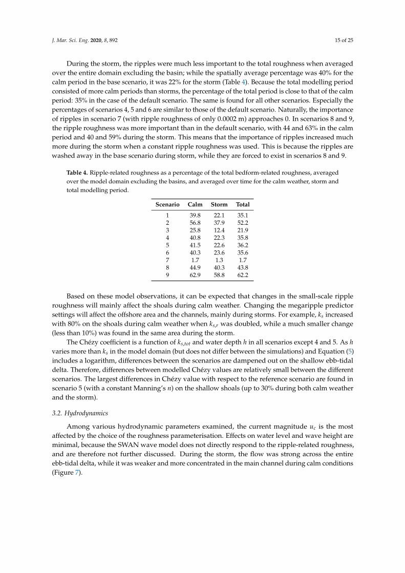
During the storm, the ripples were much less important to the total roughness when averagedover the entire domain excluding the basin; while the spatially average percentage was 40% for thecalm period in the base scenario, it was 22% for the storm (Table 4). Because the total modelling periodconsisted of more calm periods than storms, the percentage of the total period is close to that of the calmperiod: 35% in the case of the default scenario. The same is found for all other scenarios. Especially thepercentages of scenarios 4, 5 and 6 are similar to those of the default scenario. Naturally, the importanceof ripples in scenario 7 (with ripple roughness of only 0.0002 m) approaches 0. In scenarios 8 and 9,the ripple roughness was more important than in the default scenario, with 44 and 63% in the calmperiod and 40 and 59% during the storm. This means that the importance of ripples increased muchmore during the storm when a constant ripple roughness was used. This is because the ripples arewashed away in the base scenario during storm, while they are forced to exist in scenarios 8 and 9.
Table 4. Ripple-related roughness as a percentage of the total bedform-related roughness, averagedover the model domain excluding the basins, and averaged over time for the calm weather, storm andtotal modelling period.
Scenario Calm Storm Total
1 39.8 22.1 35.12 56.8 37.9 52.23 25.8 12.4 21.94 40.8 22.3 35.85 41.5 22.6 36.26 40.3 23.6 35.67 1.7 1.3 1.78 44.9 40.3 43.89 62.9 58.8 62.2
Based on these model observations, it can be expected that changes in the small-scale rippleroughness will mainly affect the shoals during calm weather. Changing the megaripple predictorsettings will affect the offshore area and the channels, mainly during storms. For example, ks increasedwith 80% on the shoals during calm weather when ks,r was doubled, while a much smaller change(less than 10%) was found in the same area during the storm.
The Chézy coefficient is a function of ks,tot and water depth h in all scenarios except 4 and 5. As hvaries more than ks in the model domain (but does not differ between the simulations) and Equation (5)includes a logarithm, differences between the scenarios are dampened out on the shallow ebb-tidaldelta. Therefore, differences between modelled Chézy values are relatively small between the differentscenarios. The largest differences in Chézy value with respect to the reference scenario are found inscenario 5 (with a constant Manning’s n) on the shallow shoals (up to 30% during both calm weatherand the storm).
3.2. Hydrodynamics
Among various hydrodynamic parameters examined, the current magnitude uc is the mostaffected by the choice of the roughness parameterisation. Effects on water level and wave height areminimal, because the SWAN wave model does not directly respond to the ripple-related roughness,and are therefore not further discussed. During the storm, the flow was strong across the entireebb-tidal delta, while it was weaker and more concentrated in the main channel during calm conditions(Figure 7).

J. Mar. Sci. Eng. 2020, 8, 892 16 of 25
Figure 7. Time-averaged value of depth-averaged current velocity magnitude (A,B), time-integratedbedload transport (C,D) and time-integrated suspended load transport (E,F) during the storm (A,C,E)and the calm weather period (B,D,F) on a select number of model grid points.
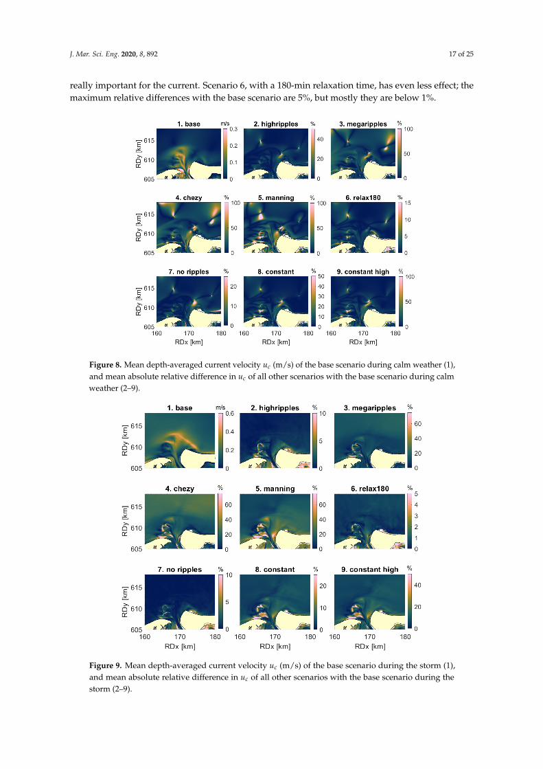
In general, a higher roughness leads to a lower current velocity. When the roughness was changed,the flow direction generally remained the same. Throughout the model domain, direction differencesbetween all scenarios and the base scenario were mostly below 5◦, with maximum values of 30◦ onthe western shoal in some scenarios. Thus, directions are not affected in such a way that the currentis reversed. Only the shape of the tidal ellipse is slightly altered by (temporal) changes in bedformroughness. The largest differences with the base scenario in both current velocity direction andmagnitude are found when a constant Chézy or Manning roughness value was prescribed, or whenthe megaripple roughness was doubled. During calm weather, in these cases relative differencesin current velocity exceeded 100%, but this only occurred at locations where the current velocity inthe base run was near 0 (Figure 8). On the delta, the current was affected by approximately 50%.During the storm, choosing a constant Manning value resulted in up to 70% relative difference incurrent velocity on the delta, while the offshore areas were affected by approximately 20% (Figure 9).Choosing a constant Chézy value resulted in 30% relative difference in the entire model domain,with maximum values near the western shoal of 70%. This is similar to the effects of prescribing adoubled megaripple roughness. The use of a constant ripple roughness (scenarios 7–9) mainly affectedthe current at the shoals. The relative differences with the base scenario were larger for larger rippleroughness, and were 40% at the most. A doubled varying ripple roughness (scenario 2) resulted in asimilar pattern, but the changes the current velocity in this case were maximum 10%. Since the effectof doubling the megaripples was much larger, it can be stated that small-scale ripples roughness is not
J. Mar. Sci. Eng. 2020, 8, 892 17 of 25
really important for the current. Scenario 6, with a 180-min relaxation time, has even less effect; themaximum relative differences with the base scenario are 5%, but mostly they are below 1%.
Figure 8. Mean depth-averaged current velocity uc (m/s) of the base scenario during calm weather (1),and mean absolute relative difference in uc of all other scenarios with the base scenario during calmweather (2–9).
Figure 9. Mean depth-averaged current velocity uc (m/s) of the base scenario during the storm (1),and mean absolute relative difference in uc of all other scenarios with the base scenario during thestorm (2–9).

J. Mar. Sci. Eng. 2020, 8, 892 18 of 25
3.3. Sediment Transport
The bed load and suspended load transport are both considered by time-integration over thecalm and storm period. The amount of suspended load transport was approximately ten to twentytimes larger than the bed load transport, but apart from that the patterns in the base scenario weresimilar (Figure 7). Most transport takes place during the storm, at the seaward extent of the ebb-tidaldelta shoals and at the inlet channel. During calm weather, less transport takes place, and it is mostlyconfined to the channel.
Similar to the current velocities, transport directions are not significantly affected by the roughnessscenario. Direction differences are a little bit larger in sediment transport than in current velocity,with the largest differences occurring on the shallow parts of the delta. In the deeper parts of the modeldomain, differences with the base scenario are in the order of 10 degrees. Especially for suspendedload transport, differences with the base scenario are found of up to 180 degrees, which means that thesediment transport direction is reversed. This happens only in areas in which the directions in the baserun also show large variations on small areas. The large differences with the base run are thus causedby the transport patterns that remains the same, but slightly shifts in space.
The patterns in relative difference in time-integrated sediment transport magnitude between thebase scenario and the other scenarios are also similar to those of uc. During calm weather, for bothbedload and suspended load transport, the relative differences with the base scenario were generallybelow 10%. Yet, values of up to 200% were found at the shallow areas, where the time-integratedamount of sediment transport in the base run approached 0 (Figures 10 and 11).
Figure 10. Time-integrated suspended load transport qs during calm weather (1), and absolute relativedifference in qs of all other scenarios with the base scenario during calm weather (2–9).

J. Mar. Sci. Eng. 2020, 8, 892 19 of 25
Figure 11. Time-integrated bedload transport qb during calm weather (1), and absolute relativedifference in qb of all other scenarios with the base scenario during calm weather (2–9).
During storm, the MARD-patterns of the bedload and the suspended load magnitude arenot similar. The time-integrated bedload transport is affected most when a constant Chézy value(scenario 4), Manning coefficient (scenario 5) or a constant high ripple roughness (scenario 9) isprescribed (Figure 12). In these cases, relative differences with the base scenario of more than 100%are found, but they occur only on the locations where the transport magnitude in the base run wasvery small. In the scenarios with high megaripple roughness (scenario 2), a constant Chézy value(scenario 4), very small ripple roughness (scenario 7) and constant high ripple roughness (scenario 9),the time-integrated bedload transport magnitude is also affected offshore by some 20–30%.
The highest relative differences with the base run are found for suspended load during the storm.Here, relative differences of more than 100% occur in all scenarios (Figure 13). The effects of changingroughness are not confined to the shoals anymore as during calm weather, but are found throughout themodel domain. Even when a relaxed ripple roughness (scenario 6) was used, relative differences of up to70% were found, even though the current was hardly affected. This implies that the change in sedimenttransport is caused by a change in sediment concentration (see Equation (9)). Apart from the scenarioswith the constant Chézy value (scenario 4) or the doubled megaripple roughness (scenario 3), the easternshoals are most affected. At this location the ripples in the base scenario made up to 60% of the totalroughness during the storm (Figure 6). The constant Chézy value was chosen based on an average depth,so offshore and in the deeper parts of the channel, where the water depth is larger than the average,the Chézy value was too high. In all other simulations, the change in transport in the channel is near 0.When the megaripple roughness was doubled, no clear effect was found on the shoals and in the channel,and a larger effect was seen offshore, in the area where megaripples are dominant. As described before,the suspended load does not directly depend on ks,mr (Figure 1), implying that the change in transport inthis scenario was caused by the changes in hydrodynamics. Lastly, it should be noted that low relativedifferences were found for all scenarios at the northern part of the delta, where the absolute values of thesuspended load transport magnitude in the base run were highest.

J. Mar. Sci. Eng. 2020, 8, 892 20 of 25
Figure 12. Time-integrated bedload transport qb during the storm (1), and absolute relative differencein qb of all other scenarios with the base scenario during the storm (2–9).
Figure 13. Time-integrated suspended load transport qs during the storm (1), and absolute relativedifference in qs of all other scenarios with the base scenario during the storm (2–9).

J. Mar. Sci. Eng. 2020, 8, 892 21 of 25
4. Discussion
The aim of this paper was to assess the effect of the roughness induced by small-scale ripples andmegaripples on hydrodynamics and sediment transport in Delft3D. First of all, the modelled rippleswere compared to measurements. Measured ripples were found to have relatively stable dimensions.Ripple heights were only weakly related to orbital velocity (which is a function of wave height andwater depth), while no relation was found at all between ripple dimensions and current velocity [17].Brakenhoff et al. [17] therefore suggested to use a constant ripple roughness in modelling. In thepresent study, the effects of a constant ripple roughness (scenarios 7, 8 and 9) were compared to thoseof the default Van Rijn roughness predictor (scenarios 2, 3 and 6) and to situations with roughnessincorporated into constant Chézy or Manning values (scenarios 4 and 5).
Figure 4 showed that the ripple-related roughness simulated by using a 180-min relaxation timewas closest to the measured roughness. Yet, this does not mean that this scenario also gives the bestresemblance of the true current and sediment transport. The current in this scenario changes with only2% with respect to the base scenario. However, no measures of sediment transport are available ofthe studied location and time period, so it is unclear if the base scenario or the relaxation scenarioperforms best.
Based on the importance of small-scale ripples and megaripples for the total roughness, it wasexpected that changes in the small-scale ripple roughness would mainly affect the shoals during calmweather, while megaripples will affect the offshore area and the channels, mainly during storms. This isalso confirmed by the model results. During calm weather, both the current and the time-integratedsediment transport are mainly affected on the shallow parts of the delta. During storm, the offshorearea is affected as well. In the deep channel in between the islands, the current depends on the chosenroughness scenario, but the transport does not. Since sediment transport q is a function of currentvelocity u and sediment concentration C, the fact that transport does not change means that higherripple roughness also causes a higher depth-integrated sediment concentration. It is expected thatthese different effects of small-scale ripples and megaripple roughness will also be found on otherebb-tidal deltas, since current and depth distributions in space will be similar (i.e., alternating shoalsand channels). Yet, differences in grain size distribution might also cause different ripple dimensionsand behaviour [17], so one should be careful in extrapolating the results to other deltaic systems.
The transport in the channel is only affected when a constant Chézy value is chosen. This isbecause this Chézy value is constant throughout the model domain, so it is not dependent on depth.Therefore, in areas deeper than the average depth, the prescribed roughness is higher than when adepth-dependent C is chosen. This is also the case on shallow areas during the storm when constantroughness values are prescribed. Both in the field data and in the model, mobility parameter ψ
often exceeds 250 during the storm, which results in the small-scale ripples being washed away.Therefore, when the ripples are forced to be constant in the model, they are too high, resulting in largeerrors in current velocity and sediment transport. Therefore, contrary to what Brakenhoff et al. [17]suggested, a constant ripple roughness should not be implemented in morphologic studies, especiallywhen shallow (<10 m) areas and/or storm periods are modelled. Davies and Robins [19] drew asimilar conclusion when studying bedforms in an estuary with TELEMAC. Even though their studyconcerned megaripples and dunes predicted by Van Rijn [3], they also found that a spatio-temporallyvarying ks resulted in the most accurate prediction of local hydrodynamics. This gives the use of theVan Rijn roughness predictor an advantage over choosing a constant ripple roughness or a constantChézy value.
The Delft3D model, similar to other numerical morphodynamic models such as MIKE21,TELEMAC and ROMS, is highly complicated and involves numerous feedbacks (see Figure 1). Whilethis resembles reality better, this also makes it difficult to say whether changes in sediment transport aremainly caused directly by changes in roughness or indirectly by changes in hydrodynamics. Figure 1shows that both causes are possible. In the scenarios with doubled small-scale ripple roughness,relaxed ripple roughness, and a constant very small ripple roughness, the current velocities during the
J. Mar. Sci. Eng. 2020, 8, 892 22 of 25
storm in most parts of the domain change with 2% or less. Yet, during storm, the suspended sedimenttransport in these scenarios changes by 60–70%. This implies that the direct effect of bedform-relatedroughness is very important: it increases the depth-integrated sediment concentration and thereforealso qs.
In short, the largest effect of roughness is found in the depth-averaged current velocity and thesuspended load transport. Changes in transport magnitude appear larger than changes in currentmagnitude. Yet, it is unknown which of the scenarios shows the most realistic amount of sedimenttransport, and although the differences with the base scenario are higher, the scenarios with theconstant ripple roughness do show similar patterns in MARD-values as the Van Rijn scenario with highripples. It therefore might be valid to use a spatio-temporally constant roughness value in exploratorystudies, when the ’true’ behaviour of the system is unknown, (e.g., determining causes for spatialpatterns or morphologic behaviour). Therefore, it is especially important to put effort into choosing aroughness predictor when transport or morphologic calculations are made, e.g., in hindcasting studies.If only hydrodynamic simulations are done, the errors are expected to remain mostly below 10%,and they will be located at the shallow areas. Only if a constant Manning’s n is prescribed, errorscan increase further, in our case the differences with the base scenario were up to 40%. On top ofthat, even with small changes in ripple-related roughness ks,r, the sediment transport magnitude stillchanges. This means that it is important to carefully consider which ripple roughness predictor is usedand that coastal models that simulate sediment transport or morphological change should incorporatespatio-temporally varying ripple roughness predictors. Also, a model user should always keep inmind that over time, small changes in the predicted ripple roughness could lead to large changes inthe predicted total sediment transport and thus morphology.
The present study is representative of the sediment transport predictor of Van Rijn [3].This predictor can also be incorporated into other models, such as TELEMAC. It is hypothesisedthat the results would be similar if a predictor was used that also calculates bedload and suspendedload transport separately. Since the present study showed that currents are affected by up to 60% whenthe roughness scenario is changed, most bedload predictors will be affected by changes in roughness.This is because in all bedload predictors, and even some total load predictors such as the one fromEngelund-Hansen [35], the transport depends on the depth-averaged current velocity to a power of 3–5.The calculation of suspended load varies more between various predictors, because it mainly dependson the calculation of the reference height. Therefore, it is advised to perform a similar sensitivity studywhen a different transport predictor is used.
Further research should also address the long-term morphodynamic feedbacks. Spatial differencesin sediment transport can lead to different morphologic development, so the effects of roughnessthat were found in the present study could be amplified or reduced by these feedbacks. Furthermore,the interaction between the different bedform scales should be addressed. Nikora et al. [36] showedthat the migration of larger bedforms (megaripples in our case) could be caused by the movementof small-scale ripples. A time series of measurements of both scales at the same location is, however,not available for our study site.
5. Conclusions
For the first time, the effect of small-scale ripples and megaripples on hydrodynamics andsediment transport was quantified in detail using Delft3D scenarios for a mixed wave-currentenvironment (Ameland ebb-tidal delta). The In Delft3D, small-scale ripples and megaripples togetherconstitute the bedform-related roughness. Although small-scale ripples are lower than megaripples,it was found that small-scale ripple-related roughness can make up to 100% of the total roughnesson shallow parts of the ebb-tidal delta. Megaripples are more important in the current-dominatedchannel and further offshore. The bedforms were found to affect the current velocity and sedimenttransport on the shallow parts of the ebb-tidal delta. Current velocity magnitudes affected by differentbedform roughness scenarios resulted in overall differences of 10–20%, both during calm weather

J. Mar. Sci. Eng. 2020, 8, 892 23 of 25
and during storm. In sediment transport, on the other hand, small changes in predicted rippleroughness lead to changes of more than 100%. Transport and flow directions were not significantlyaffected. During a storm, small-scale ripples are predicted to be washed away, but megaripplesremain. This process cannot be simulated if a constant roughness value is prescribed, leading tooverestimations in sediment transport. Therefore, it is advised to use a spatio-temporally variablebedform roughness in morphodynamic simulations in Delft3D. Future research should address thelong-term morphodynamic feedbacks and the interaction between the different bedform scales.
Author Contributions: Conceptualization, all; methodology, L.B., B.G., J.v.d.W. and R.S.; software, L.B. and R.S.;validation, B.G., J.v.d.W., M.v.d.V. and G.R.; formal analysis, L.B.; investigation, L.B.; resources, B.G., J.v.d.W.and R.S.; data curation, J.v.d.W.; writing–original draft preparation, L.B.; writing–review and editing, all;visualization, L.B.; supervision, M.v.d.V. and G.R.; project administration, L.B.; funding acquisition, M.v.d.V.All authors have read and agreed to the published version of the manuscript.
Funding: This project is part of the research program SEAWAD, a ‘Collaboration Program Water’ with projectnumber 14489, which is financed by the Netherlands Organisation for Scientific Research (NWO) Domain Appliedand Engineering Sciences, and co-financed by Rijkswaterstaat (Ministry of Infrastructure and Water Managementin The Netherlands). The measurement campaign was co-financed by Rijkswaterstaat as well, in the context of theCoastal Genesis 2.0 project. The PhD project of LB is financed by the SEAWAD project.
Acknowledgments: The scientific colour map batlow [37] is used in this study to prevent visual distortion of thedata and exclusion of readers with colour-vision deficiencies [38]. The authors would like to thank Bert Jagers forhis help with clarifying the processes incorporated in Delft3D and the creation of a version in which we couldsimulate constant ripple roughness. Rinse de Swart is thanked for his invaluable help when all was lost. We wouldlike to thank Gerald Herrling, Robert Bialik and 2 anonymous reviewers for their constructive reviews of theinitial manuscript.
Conflicts of Interest: The authors declare no conflict of interest. The funders had no role in the design of thestudy; in the collection, analyses, or interpretation of data; in the writing of the manuscript, or in the decision topublish the results.
References
1. Lefebvre, A.; Ernstsen, V.; Winter, C. Influence of compound bedforms on hydraulic roughness in a tidalenvironment. Ocean. Dyn. 2011, 61, 2201–2210. [CrossRef]
2. Van Rijn, L. Equivalent roughness of alluvial bed. J. Hydraul. Div. ASCE 1982, 108, 1215–1218.3. Van Rijn, L. Unified View of Sediment Transport by Currents and Waves. I: Initiation of Motion,
Bed Roughness, and Bed-Load Transport. J. Hydraul. Eng. 2007, 133, 649–667. [CrossRef]4. Van Der A, D.A.; Ribberink, J.S.; Van Der Werf, J.J.; O’Donoghue, T.; Buijsrogge, R.H.; Kranenburg, W.
Practical sand transport formula for non-breaking waves and currents. Coast. Eng. 2013, 76, 26–42.[CrossRef]
5. O’Donoghue, T.; Doucette, J.; van der Werf, J.; Ribberink, J. The dimensions of sand ripples in full-scaleoscillatory flows. Coast. Eng. 2006, 53, 997–1012. [CrossRef]
6. Dastgheib, A.; Roelvink, J.; Wang, Z. Long-term process-based morphological modeling of the MarsdiepTidal Basin. Mar. Geol. 2008, 256, 90–100. [CrossRef]
7. Lenstra, K.; Pluis, S.; Ridderinkhof, W.; Ruessink, B.; van der Vegt, M. Cyclic channel-shoal dynamics atthe Ameland inlet: The impact on waves, tides, and sediment transport. Ocean. Dyn. 2019, 69, 409–425.[CrossRef]
8. Iglesias, I.; Avilez-Valente, P.; Bio, A.; Bastos, L. Modelling the Main Hydrodynamic Patterns in ShallowWater Estuaries: The Minho Case Study. Water 2019, 11, 1040. [CrossRef]
9. Herrling, G.; Winter, C. Morphological and sedimentological response of a mixed-energy barrier island tidalinlet to storm and fair-weather conditions. Earth Surf. Dyn. 2014, 2, 363–382. [CrossRef]
10. Zavala-Garay, J.; Theiss, J.; Moulton, M.; Walsh, C.; van Woesik, R.; Mayorga-Adame, C.; García-Reyes, M.;Mukaka, D.; Whilden, K.; Shaghude, Y.W. On the dynamics of the Zanzibar Channel. JGR Oceans 2015,120, 6091–6113. [CrossRef]
11. Ralston, D.; Talke, S.; Geyer, W.; Al-Zubaidi, H.; Sommerfield, C. Bigger Tides, Less Flooding: Effects ofDredging on Barotropic Dynamics in a Highly Modified Estuary. J. Geophys. Res. Ocean. 2019, 124, 196–211.[CrossRef]

J. Mar. Sci. Eng. 2020, 8, 892 24 of 25
12. Elias, E.P.L.; Hansen, J.E. Understanding processes controlling sediment transports at the mouth of a highlyenergetic inlet system (San Francisco Bay, CA). Mar. Geol. 2013, 345, 207–220. [CrossRef]
13. Wengrove, M.E.; Foster, D.L.; Lippmann, T.C.; de Schipper, M.A.; Calantoni, J. Observations ofTime-Dependent Bedform Transformation in Combined Wave-Current Flows. J. Geophys. Res. Ocean.2018, 123, 7581–7598. [CrossRef]
14. Lefebvre, A.; Ernstsen, V.; Winter, C. Bedform characterization through 2D spectral analysis. J. Coast. Res.2011, SI64, 781–785.
15. Ganju, N.; Sherwood, C. Effect of roughness formulation on the performance of a coupled wave,hydrodynamic, and sediment transport model. Ocean. Model. 2010, 33, 299–313. [CrossRef]
16. Nelson, T.; Voulgaris, G.; Traykovski, P. Predicting wave-induced ripple equilibrium geometry. J. Geophys.Res. Ocean. 2013, 118, 3202–3220. [CrossRef]
17. Brakenhoff, L.; Kleinhans, M.; Ruessink, B.; van der Vegt, M. Spatio-temporal characteristics of small-scalewave-current ripples on the Ameland ebb-tidal delta. Earth Surf. Process. Landforms 2020. [CrossRef]
18. Idier, D.; Astruc, D.; Hulscher, S. Influence of bed roughness on dune and megaripple generation.Geophys. Res. Lett. 2004, 31. [CrossRef]
19. Davies, A.; Robins, P. Residual flow, bedforms and sediment transport in a tidal channel modelled withvariable bed roughness. Geomorphology 2017, 295, 855–872. [CrossRef]
20. Lesser, G.; Roelvink, J.; van Kester, J.; Stelling, G. Development and validation of a three-dimensionalmorphological model. Coast. Eng. 2004, 51, 883–915. [CrossRef]
21. van Rijn, L.; Walstra, D.; van Ormondt, M. Description of TRANSPOR2004 and Implementation inDelft3D-ONLINE; Techreport Z3748.10; WL | Delft Hydraulics: Delft, The Netherlands, 2004.
22. Marriott, M.; Jayaratne, R. Hydraulic roughness—Links between Manning’s coefficient, Nikuradse’sequivalent sand roughness and bed grain size. In Proceedings of Advances in Computing and Technology,(AC&T) The School of Computing and Technology 5th Annual Conference; University of East London: London,UK, 2010; pp. 27–32.
23. Booij, N.; Ris, R.C.; Holthuijsen, L.H. A third-generation wave model for coastal regions: 1. Modeldescription and validation. J. Geophys. Res. Ocean. 1999, 104.C4, 7649–7666. [CrossRef]
24. Ris, R.C.; Holthuijsen, L.H.; Booij, N. A third-generation wave model for coastal regions: 2. Verification.J. Geophys. Res. Ocean. 1999, 104.C4, 7667–7681. [CrossRef]
25. Nederhoff, C.; Schrijvershof, R.; Tonnon, P.; van der Werf, J. The Coastal Genesis II Terschelling–Ameland Inlet(CGII-TA) Model; Techreport 1220339-008-ZKS-0004; Deltares: Delft, The Netherlands, 2019. Available onlineat: http://publications.deltares.nl/1220339_008.pdf (accessed on 8 November 2020).
26. Galappatti, G.; Vreugdenhil, C. A depth-integrated model for suspended sediment transport. J. Hydraul. Res.1985, 23, 359–377. [CrossRef]
27. Van Rijn, L. Unified View of Sediment Transport by Currents and Waves. II: Suspended Transport.J. Hydraul. Eng. 2007, 133, 668–689. [CrossRef]
28. Van Rijn, L. Principles of Sediment Transport in Rivers, Estuaries and Coastal Seas; Aqua Publications Amsterdam:Amsterdam, The Netherlands, 1993; Volume 1006.
29. Lesser, G. An Approach to Medium-Term Coastal Morphological Modelling. Ph.D. Thesis, IHE DelftInstitute for Water Education, Delft, The Netherlands, 2009.
30. Nederhoff, C.; Schrijvershof, R.; Tonnon, P.; Van Der Werf, J.; Elias, E. Modelling hydrodynamics in theAmeland inlet as a basis for studying sand transport. Coast. Sediments 2019, 1971–1983. [CrossRef]
31. van Prooijen, B.; Tissier, M.; de Wit, F.; Pearson, S.; Brakenhoff, L.; van Maarseveen, M.; van der Vegt, M.;Mol, J.; Kok, F.; Holzhauer, H.; et al. Measurements of Hydrodynamics, Sediment, Morphology and Benthoson Ameland Ebb-Tidal Delta and Lower Shoreface. Earth Syst. Sci. Data 2020. [CrossRef]
32. Zijl, F.; Verlaan, M.; Gerritsen, H. Improved water-level forecasting for the Northwest European Shelf andNorth Sea through direct modelling of tide, surge and non-linear interaction. Ocean. Dyn. 2013, 63, 823–847.[CrossRef]
33. Pearson, S.; van Prooijen, B.; de Wit, F.; Meijer-Holzhauer, H.; de Looff, A.; Wang, Z. Observations ofsuspended particle size distribution on an energetic ebb-tidal delta. Coast. Sediments 2019. [CrossRef]
34. Duran-Matute, M.; Gerkema, T. Calculating Residual Flows through a Multiple-Inlet System: TheConundrum of the Tidal Period. Ocean. Dyn. 2015, 65, 1461–1475. [CrossRef]
J. Mar. Sci. Eng. 2020, 8, 892 25 of 25
35. Engelund, F.; Hansen, E. A Monograph on Sediment Transport in Alluvial Streams; Technical University ofDenmark Ostervoldgade 10; Copenhagen K: Lyngby, Denmark, 1967.
36. Nikora, V.I.; Sukhodolov, A.N.; Rowinski, P.M. Statistical sand wave dynamics in one-directional waterflows. J. Fluid Mech. 1997, 351, 17–39. [CrossRef]
37. Crameri, F. Scientific Colour Maps. Zenodo 2019. [CrossRef]38. Crameri, F. Geodynamic diagnostics, scientific visualisation and StagLab 3.0. Geosci. Model Dev. 2018,
11, 2541–2562. [CrossRef]
Publisher’s Note: MDPI stays neutral with regard to jurisdictional claims in published maps and institutionalaffiliations.
c© 2020 by the authors. Licensee MDPI, Basel, Switzerland. This article is an open accessarticle distributed under the terms and conditions of the Creative Commons Attribution(CC BY) license (http://creativecommons.org/licenses/by/4.0/).